electrochemical potential - uio.no · 7. electrochemical transport 7.2 flux equations – wagner...

7. Electrochemical transport

7.1


Electrochemical potential

In the chapter on diffusion we learned that random diffusion is driven by thermal energy and that it in crystalline solids requires defects. Moreover, we learned that a net flux of a species can result from a gradient in its chemical potential. In the chapter on electrical conductivity we furthermore saw that a net flux of charged particles would result in a gradient of electrical potential.

In ionic media (materials, liquids, and solutions) the chemical and electrical potentials act simultaneously, and it is often convenient to combine them into an electrochemical potential. For the species i we have

φµη ez+= iii (7.1)

This is true whether the species is real or a defect, but in general we shall onwards deal mainly with real species and real charges zi.

The electrochemical potential gradient is accordingly, in the one-dimensional case,

dxdez+

dxd

=dxd

iii φµη

(7.2)

The combination of chemical and electrical potentials and potential gradients forms the basis for the treatment of all mass transport processes involving charged species (ions) in ionic solids, and is the theme of this chapter. The theory is termed Wagner-type after Carl Wagner, who was the first to derive it, originally to describe oxidation of metals.


7.2

Flux equations – Wagner theory

General derivation of Wagner-type flux expressions

We have seen in a preceding paragraph that a force, expressed as gradient in a potential Pi acting on a species i, gives rise to a flux density of that species which is proportional to its self-diffusion coefficient Di. By assuming that the potential acting is the electrochemical potential, we obtain

]dxdez+

dxd

[kT

cD-=dxd

kTcD-

dxPd

kTcD-=j i

iiiiiiiiii

φµη= (7.3)

Via the Nernst-Einstein equation we may substitute conductivitiy for the random diffusivity and obtain the following alternative expression for the flux density:

]dxdez+

dxd

[ez

-=j i

i

i

ii

φµσ2)(

(7.4)

If the species is charged, the flux density for i gives rise to a partial current density ii:

]dxdez+

dxd

[ez

-=jez=i ii

i

iiii

φµσ (7.5)

The net current density in the sample is obtained by summing the partial current densities over all the species k:

]dxdez+

dxd

[ez

-=jez=i kk

k

kkkkktot

φµσ∑∑ (7.6)

The sample is next assumed to be connected to an external electric circuit. This may be real, with electrodes and wires and an electrical supply or load, or it may be absent, in which case we say that we have an open circuit. Since the sample makes a series connection with the external circuit, the currect in the sample must be the same as in the external circuit.


7.3

For a bare sample, a gas permeation membrane, or for an open-circuit fuel cell or other electrochemical device, the total current is zero. For fuel cells or electrolysers in operation, on the other hand, the current is non-zero.

By using the definition of total conductivity, kktot = σσ ∑ , and the definition of transport

number, kk

k

tot

kk =t σ

σσσ

∑= , we obtain the following very important expression:

dxd

ezt-i-=

dxd k

k

kk

tot

tot µσ

φ∑ (7.7)

This relates the electrical potential gradient to the total (net, external) current density, the total conductivity, and the transport number and chemical potential gradient of all charge carriers.

From charged to neutral species: the electrochemical reaction

The chemical potentials of charged species are not well-defined, and we need to represent them instead by chemical potentials of neutral species. For this purpose we may assume equilibria between neutral and charged species and electrons, i.e. in the electrochemical red-ox- reaction

−ze+S=S z (7.8)

where S is a neutral chemical entity and z may be positive or negative. The equilibrium condition for this is expressed in terms of the chemical potentials of products and reactants:

0=− µµµ SeS dzd+d -z (7.9)

and can be rearranged with respect to the ionic species:

µµµ eSS -z zddd −= (7.10)


7.4

We insert this for all ionic species n in the expression for the electrical potential gradient. The entry (among k) for electrons is left unsubstituted. By using 1=∑ kk t we obtain

dxd

e1+

dxd

ezt-i-=

dxd en

n

nn

tot

tot µµσ

φ∑ (7.11)

for which the chemical potentials now refer to the neutral forms of each carrier.

The voltage over a sample

We now integrate the electrical potential gradient over the thickness of the sample, from side 1 to side 2, in order to obtain the voltage over the sample:

∫∫∫∫ ∑−II

Ie

II

In

n

nn

II

I tot

totII

I

de1+d

ezt-dxi=d µµ

σφ (7.12)

)(1,, µµµ

σφφ IeIIe

II

In

n

nn

II

I tot

totIII e

+dez

t-dxi= −∑−− ∫∫ (7.13)

We further assume that the voltage is measured on each side using the same inert metal, e.g. Pt. This eliminates the difference between chemical potentials of electrons on the two sides, and the voltage measured between the two sides is

∫∫ ∑−−=−

II

In

n

nn

II

I tot

totIIIIII d

ezt-dxi=U µ

σφφ (7.14)

Under open circuit conditions, itot=0, and we obtain


7.5

∫∑=−

II

In

n

nnIII d

ezt-U µ (7.15)

We shall later see how this is used to calculate transport numbers based on open circuit voltage measurements of cells exposed to a well-defined gradient in chemical activities. Alternatively, if tn is known to be unity for ionic charge carriers this expression will yield the open circuit voltage of a fuel cell or a galvanic sensor.

If current is drawn from the sample, as in a fuel cell or battery under load, we need to know how itot varies with x. If we assume that it is constant, we get

∫∫ ∑−=∑−=−

II

In

n

nntottot

II

In

n

nn

tot

totIII d

ezt-rid

ezt-XiU µµ

σ (7.16)

where X is the thickness of the sample and rtot is the area-specific resistance of the sample. Alternatively, itotrtot (current density and area specific resistance) may be replaced by RI, (sample resistance and current):

∫∑−=−

II

In

n

nnIII d

ezt-IRU µ (7.17)

The voltage of a fuel cell or battery is thus composed of a thermodynamic part that arises from the chemical gradient, and the well-known “IR”-term which arises from the limiting kinetics (transport) in the sample. The letters “IR” may be taken to reflect current times resistance, or to mean “internal resistance”. We will later see that the direction of the current ends up such that the IR-term reduces the voltage over the fuel cell or battery.

Flux of a particular species


7.6

One of the general expression for the electrical potential gradient can now be inserted in an expression for the flux density of an individual species (Eq. 7.4) or the corresponding partial current density (Eq. 7.5). Since these two sum over chemical potential gradients of charged species, we may conveniently use Eq. 7.7 for our purpose. Inserting this into Eq. 7.4 and rearranging yields

]dx

dztzdx

d[

ezezit

=j k

k

kki

i

i

i

i

totii

µµσ∑−− 2)(

(7.18)

The first term in the right hand side simply says what we expect: If there is a net current, a flux density of species i will be set up proportional to the total current density and the transport number ti, divided by the species’ charge.

The equation above is a rather general expression that we can use to calculate flux densities of one charged species in the company of many other species. However, it reflects the flux density and gradients and properties at a particular point through the membrane. The gradients will adjust according to the varying materials properties so as to maintain a constant flyx density everywhere – what we call steady state. In order to implement this, we integrate the flux density expression over the thickness of the membrane and require that the flux density remains constant:

∫∫∫ ∑−−=II

Ik

k

kkii

i

iII

I i

totii

II

Ii ]d

ztz[d

ezdx

ezit

Xj=dxj µµσ

2)( (7.19)

If the transport number ti and the total current density itot can be taken as constant through the membrane we further obtain:

∫ ∑−−II

Ik

k

kkii

i

i

i

totii ]d

ztz[d

ezX

ezit

=Xj µµσ

2)( (7.20)


7.7

Wagner-type transport theory case studies

Oxides with transport of oxide ions and electrons

General equations

We will now apply the general theory to a number of cases. The cases we will consider first is an oxide that conducts oxygen ions and electrons. Flux equations for the two are

]dxde

dxd

[e

-=j OO

Oφµσ

24

22

2 2 −−−

− (7.21)

]dxde

dxd

[e

-=j ee

eφµσ

−−−

− 2 (7.22)

By summing up the currents from the two we obtain (as in Eq. 7.7) the expression for the potential gradient:

dxd

et

dxd

eti-=

dxd eeOO

tot

tot µµσ

φ −−−−

++22

2 (7.23)

In order to relate the potantial gradient to the chemical potential of neutral species we introduce electrochemical equilibria between neutral and charged species of oxygen:

O2e4+(g)O 22

−− = (7.24)

for which equilibrium can be expressed by

O2d

e4d+Od 2

2(g) −− = µµµ (7.25)


7.8

Introducing this we get

dxd

et

dxd

et

dxd

eti-=

dxd eeeOgOO

tot

tot µµµ

σφ −−−−−

+++2

22 )(

4 (7.26)

and knowing that the sum of transport numbers for oxygen ions and electrons in the oxide we have defined is unity, we further get

dxd

edxd

eti-=

dxd egOO

tot

tot µµ

σφ −−

++ 14

)(22

(7.27)

whereby we have exemplified Eq. 7.11. We now integrate over the thickness of the sample to obtain the voltage over it, eliminating the chemical potential of electrons (as in Eq. 7.14 and onwards):

∫ −+−=−

II

IgOOIII dte

IRU µ )(22

41

(7.28)

Using

222ln0

)()( OgOgO pkT+= µµ (7.29)

22ln)( OgO pkTdd =µ (7.30)

we get

∫ −+−=−

II

IOOIII pdte

kTIRU2

2 ln4

(7.31)

If tO −2 is independent of the oxygen partial pressure, or if we can assume as an approximation that an average tO −2 is constant over the pressure range applied, then


7.9

NOIO

IIO

OIII EtIRpp

ekT

tIRU −− +−=+−=− 2

2

22 ln

4 (7.32)

where EN is the Nernst-voltage of the oxygen concentration cell.

Open circuit voltage of concentration cell for transport number measurements

The equation above can be used to measure the average oxygen ion transport number, by measuring the open circuit voltage (OCV) over a sample exposed to a small, well-defined gradient in partial pressure of oxygen:

N

IIIO E

Ut −=−2 (7.33)

Galvanic oxygen sensor

By using a material with 12 =−tO , i.e. a solid electrolyte, and a well-defined reference

partial pressure of oxygen, the OCV can be used for measuring an unknown partial pressure:

RefRef2

2ln4 O

IIO

II pp

ekTU =− (7.34)

Fuel cell

If we apply a solid electrolyte with 12 =−tO and expose it to a gradient in oxygen partial

pressure, we get


7.10

NIO

IIO

III EIRpp

ekTIRU +−=+−=−

2

2ln4

(7.35)

This would be the voltage of a fuel cell. With I = 0, we obtain the OCV of the cell to be the Nernst voltage, of course. We furthermore see that the cell voltage diminishes due to the IR loss at increasing current, I. A plot of U vs I gives –R as the slope.

The power delivered by the cell is the current multiplied with the voltage;

NIERIUIP +−== 2 (7.36)

and it goes through a maximum at U=EN/2. Under these conditions, the power is split half-half between external work and internal loss, so the electrical efficiency is 50%. The efficiency increases as the power and current decrease, and commonly fuel cells are designed to run at ca. U=2/3 EN.

Mixed conducting oxygen permeable membrane

Now we will show how we obtain the flux of oxygen through a mixed conducting oxygen membrane material. As mentioned in the general section this is done by inserting the electrical potential gradient back into the flux equation for oxygen ions. Using e.g. Eqs. 7.21, 7.23, and 7.25 we get:

dxd

et

eit

]dx

ddx

d[

et

eit

j gOeOtotOeOeOtotOO

µσµµσ )(22

222222

2

822

42

−−−−−−−−

− −−=−−−= (7.37)

The steady state restriction is introduced by integrating over the thickness of the membrane:

µσ

)(2 2

22

22

82 gO

II

I

eOII

I

totOO

II

IO d

et

dxeit

Xjdxj ∫∫∫−−−

−− −−== (7.38)


7.11

pdtXe

kTdxteXij O

II

IeO

II

IO

totO 2

222 ln82 2 ∫∫ −−−− −−= σ (7.39)

If itot is not zero, i.e., some external current is drawn, then the first term says that the oxygen ion flux is proportional to that current and to the oxygen ion transport number. If the latter is independent of x, then the integral is straightforward. The last term adds to the flux; it is driven by an oxygen pressure gradient, and it is proportional to the oxygen ion conductivity and the transport number of electrons. This term describes permeation of oxygen ions, requiring transport of both oxygen ions and electrons. Moreover, it is inversely proportional to the thickness of the sample, X. Under open circuit conditions we may simplify to get:

pdttXe

kTpdtXe

kTj O

II

IeOtotO

II

IeOO 2

22

22 ln8

ln8 22 ∫∫ −−−−− −=−= σσ (7.40)

We now apply our derived expression for the example case of an oxygen-deficient oxide MO1-x. This contains oxygen vacancies compensated by electrons, and we have earlier shown that the

defect concentrations are given by 6/13/1/2

)4(2 −••••== OvO pK][vn

O. Since the mobility of electrons

is usually much higher than that of ionic defect, and with similar concentrations of electrons and oxygen vacancies, we may assume that the material is mainly an n-type electronic conductor.

Therefore 1≈−et . Furthermore, 6/1

0 22 2 −•• === ••••− OvOvOp]ue[v

OOσσσ , and when we insert these in

the flux expression we obtain

pdpXe

kTj O

II

IOO 22

2 ln8

6/12

0 ∫ −−=−

σ (7.41)

We substitute 2

2

2

1ln OO

O dpp

pd = and obtain


7.12

pdpXe

kTj O

II

IOO 22

26/7

20

8 ∫ −−=−

σ (7.42)

which integrates into

6/16/12

0 )()(86

222

−− −=−IO

IIOO pp

XekT

jσ

(7.43)

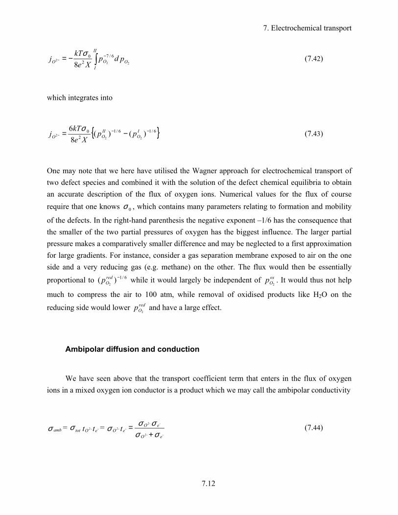
One may note that we here have utilised the Wagner approach for electrochemical transport of two defect species and combined it with the solution of the defect chemical equilibria to obtain an accurate description of the flux of oxygen ions. Numerical values for the flux of course require that one knows 0σ , which contains many parameters relating to formation and mobility

of the defects. In the right-hand parenthesis the negative exponent –1/6 has the consequence that the smaller of the two partial pressures of oxygen has the biggest influence. The larger partial pressure makes a comparatively smaller difference and may be neglected to a first approximation for large gradients. For instance, consider a gas separation membrane exposed to air on the one side and a very reducing gas (e.g. methane) on the other. The flux would then be essentially

proportional to 6/1)(2

−redOp while it would largely be independent of ox

Op2. It would thus not help

much to compress the air to 100 atm, while removal of oxidised products like H2O on the

reducing side would lower redOp

2 and have a large effect.

Ambipolar diffusion and conduction

We have seen above that the transport coefficient term that enters in the flux of oxygen ions in a mixed oxygen ion conductor is a product which we may call the ambipolar conductivity

σσσσσσσ

+=

eO

eOeOeOtotamb

--2

--2--2--2 t=tt= (7.44)


7.13

This reflects the fact that so-called ambipolar conduction of two species is necessary (in this case for charge compensation).

The corresponding terms transformed to diffusivities are called the ambipolar diffusion coefficients for oxygen:

tD=D eOamb --2 (7.45)

Such terms, like partial conductivity and self-diffusion, reflect thermal random mobility as before, but are restricted by the slower of the two ambipolar diffusing species (ions or electrons).

Many other cases of combined transport coefficients are in use, e.g. the combined (additive) transport of oxygen and metal ions commonly that we shall address later (and exemplify by the high temperature oxidation of metals), the combination of two diffusivities involved in interdiffusion (mixing) processes, and the mass transport in creep being rate limited by the smallest out of cation and anion diffusivities in a binary compound. As some of these sometimes are referred to as ambipolar or chemical diffusivities, we want to stress the above simple definition of ambipolar transport coefficients as relevant for membrane applications using mixed conductors.

Chemical diffusion and tracer diffusion

General case

The chemical diffusion coefficient is the phenomenological coefficient that enters a Fick's 1st law of diffusion in a concentration gradient:

dxdc

D-=j iii

~ (7.46)


7.14

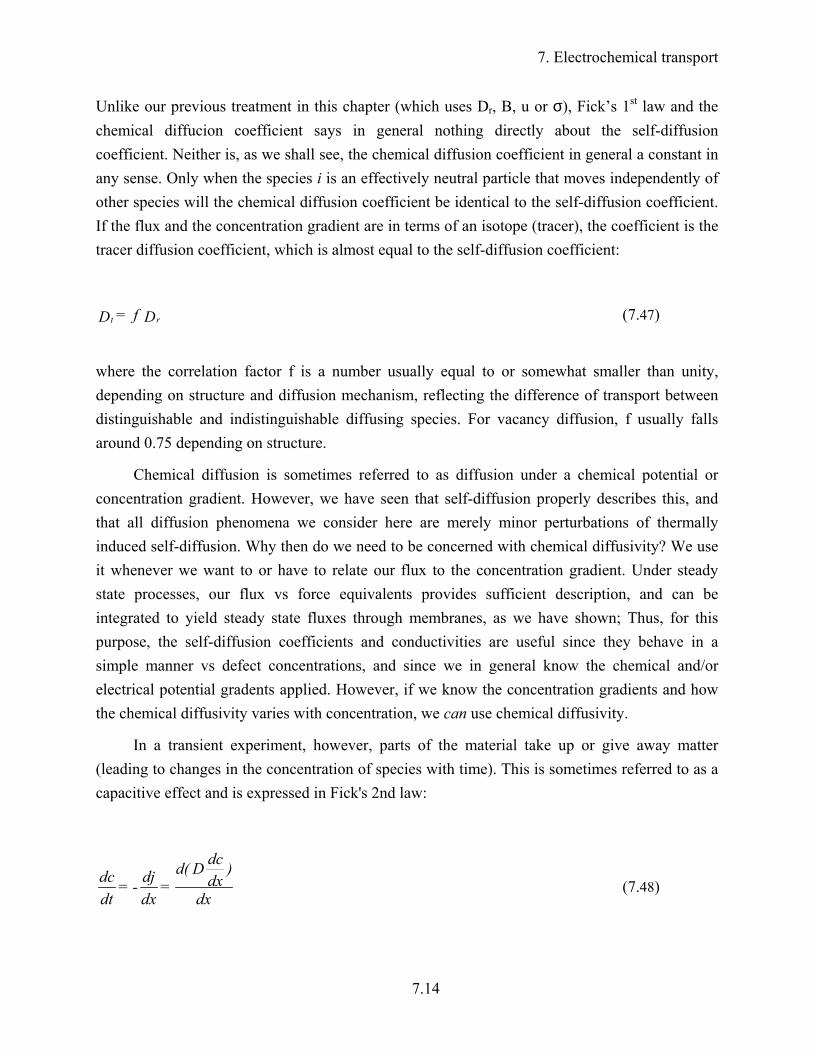
Unlike our previous treatment in this chapter (which uses Dr, B, u or σ), Fick’s 1st law and the chemical diffucion coefficient says in general nothing directly about the self-diffusion coefficient. Neither is, as we shall see, the chemical diffusion coefficient in general a constant in any sense. Only when the species i is an effectively neutral particle that moves independently of other species will the chemical diffusion coefficient be identical to the self-diffusion coefficient. If the flux and the concentration gradient are in terms of an isotope (tracer), the coefficient is the tracer diffusion coefficient, which is almost equal to the self-diffusion coefficient:

Df=D rt (7.47)

where the correlation factor f is a number usually equal to or somewhat smaller than unity, depending on structure and diffusion mechanism, reflecting the difference of transport between distinguishable and indistinguishable diffusing species. For vacancy diffusion, f usually falls around 0.75 depending on structure.

Chemical diffusion is sometimes referred to as diffusion under a chemical potential or concentration gradient. However, we have seen that self-diffusion properly describes this, and that all diffusion phenomena we consider here are merely minor perturbations of thermally induced self-diffusion. Why then do we need to be concerned with chemical diffusivity? We use it whenever we want to or have to relate our flux to the concentration gradient. Under steady state processes, our flux vs force equivalents provides sufficient description, and can be integrated to yield steady state fluxes through membranes, as we have shown; Thus, for this purpose, the self-diffusion coefficients and conductivities are useful since they behave in a simple manner vs defect concentrations, and since we in general know the chemical and/or electrical potential gradents applied. However, if we know the concentration gradients and how the chemical diffusivity varies with concentration, we can use chemical diffusivity.

In a transient experiment, however, parts of the material take up or give away matter (leading to changes in the concentration of species with time). This is sometimes referred to as a capacitive effect and is expressed in Fick's 2nd law:

dx

)dxdcDd(

=dxdj-=

dtdc (7.48)


7.15

If D is independent of c and thus of x and t, then we can simplify to obtain:

dxcdD=

dxdj-=

dtdc

2

2

(7.49)

Mathematical solutions for interpretation of transient tracer, thermogravimetric and electrical conductivity experiments are based on this. The diffusion coefficient obtained is the tracer diffusion coefficient in case of a transient in isotope composition (whether measured radiographically, mass spectrometrically, thermogravimetrically or electrically) or chemical diffusion coefficients in case of a transient in chemical composition (measured thermogravimetrically or electrically or by other means). The latter is usually executed by stepping the oxygen activity by gas composition, total pressure, or electrochemical means.

It may be noted that certain tracer experiments actually yield an interdiffusion coefficient between two tracers. The diffusion coefficient for oxygen in practice cannot and need not distinguish between the different isotopes in use (usually 18O and 16O, more rarely 17O). However, for protons, the difference to deuteron (or triton) transport coefficients is considerable (e.g. a factor of 2) and should be taken into account when interpreting the results.

The multitude of transport coefficients collected can thus be divided into self-diffusion types (total or partial conductivities and mobilities obtained from equilibrium electrical measurements, ambipolar or self-diffusion data from steady state flux measurements through membranes), tracer-diffusivities, and chemical diffusivities from transient measurements. All but the last are fairly easily interrelated through definitions, the Nernst-Einstein relation, and the correlation factor. However, we need to look more closely at the chemical diffusion coefficient. We will do this next by a specific example, namely within the framework of oxygen ion and electron transport that we have restricted ourselves to at this stage.

Chemical diffusivity in the case of mixed oxygen vacancy and electronic conductor

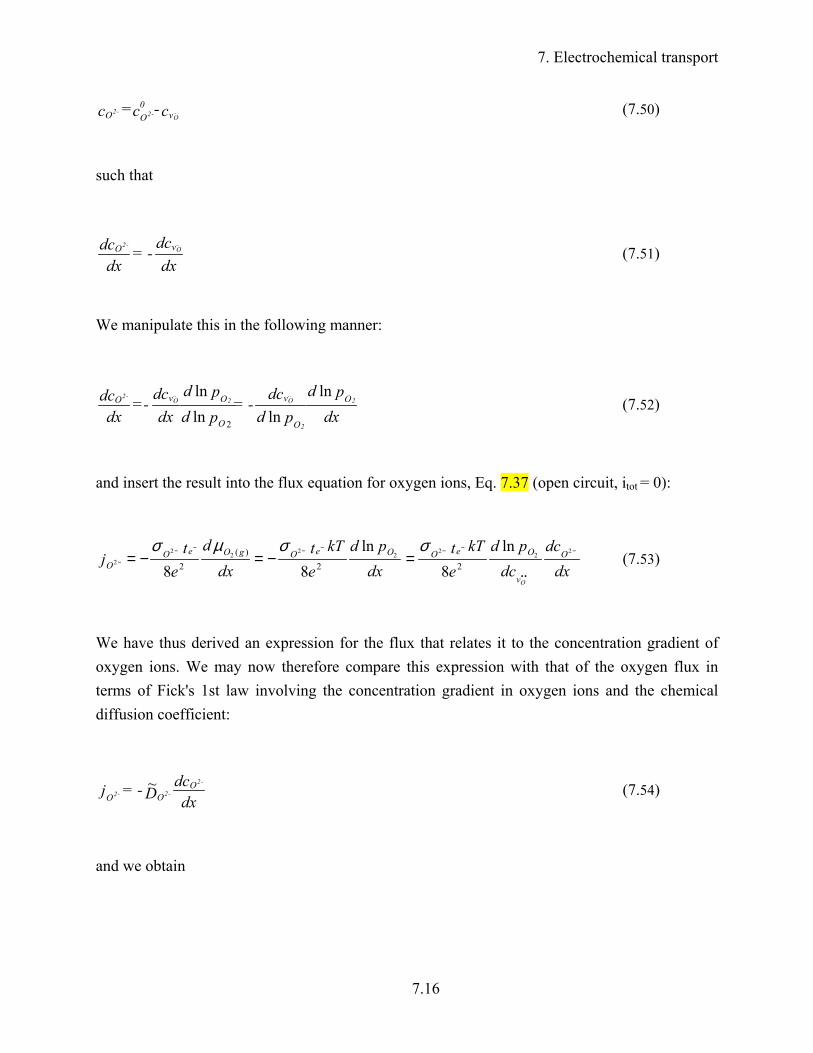
In a system with oxygen vacancies as the only oxygen point defects, the concentration of oxygen ions is the concentration of oxygen sites minus the concentration of vacancies:


7.16

c-c=c v0OO ..

O-2-2 (7.50)

such that

dxdc-=

dxdc vO ..

O-2

(7.51)

We manipulate this in the following manner:

dxpd

pddc-=

pdpd

dxdc-=

dxdc O

O

v

O

OvO 2

2

..O2

..O

-2 lnlnln

ln

2

(7.52)

and insert the result into the flux equation for oxygen ions, Eq. 7.37 (open circuit, itot = 0):

dxdc

dcpd

ekTt

dxpd

ekTt

dxd

et

j O

v

OeOOeOgOeOO

O

−

••

−−−−−−

− =−=−=2222222

2

ln8

ln88 22

)(2

σσµσ (7.53)

We have thus derived an expression for the flux that relates it to the concentration gradient of oxygen ions. We may now therefore compare this expression with that of the oxygen flux in terms of Fick's 1st law involving the concentration gradient in oxygen ions and the chemical diffusion coefficient:

dxdc

D-=j OOO

-2

-2-2~ (7.54)

and we obtain


7.17

••

−−−=

O

-2

v

OeOO dc

pde

kTtD 22 ln

8~

2

σ (7.55)

Further, by using the Nernst-Einstein-relation and inserting the relation cD=cD VVOO ..O

..O

-22 we get

2

22222

ln

ln2

lnln

2ln

2ln

2~

O

v

ev

v

Oev

v

Oevv

v

OeOOO

pd

cdtD

cdpdtD

dcpdtcD

dcpdtcD

DO

O

O

O

O

OO

O

-2

••

−••

••

−••

••

−••••

••

−−−−=−=−=−= (7.56)

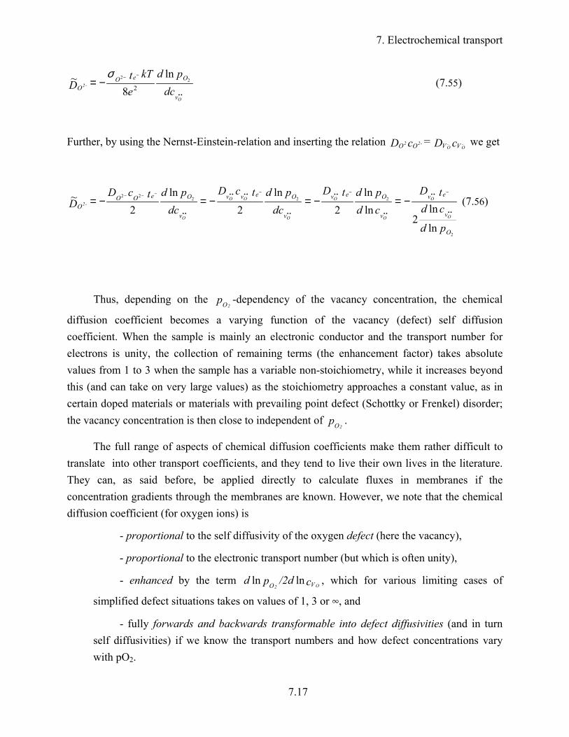
Thus, depending on the pO2-dependency of the vacancy concentration, the chemical

diffusion coefficient becomes a varying function of the vacancy (defect) self diffusion coefficient. When the sample is mainly an electronic conductor and the transport number for electrons is unity, the collection of remaining terms (the enhancement factor) takes absolute values from 1 to 3 when the sample has a variable non-stoichiometry, while it increases beyond this (and can take on very large values) as the stoichiometry approaches a constant value, as in certain doped materials or materials with prevailing point defect (Schottky or Frenkel) disorder; the vacancy concentration is then close to independent of pO2

.

The full range of aspects of chemical diffusion coefficients make them rather difficult to translate into other transport coefficients, and they tend to live their own lives in the literature. They can, as said before, be applied directly to calculate fluxes in membranes if the concentration gradients through the membranes are known. However, we note that the chemical diffusion coefficient (for oxygen ions) is

- proportional to the self diffusivity of the oxygen defect (here the vacancy),

- proportional to the electronic transport number (but which is often unity),

- enhanced by the term c/2dpd VO O2lnln , which for various limiting cases of

simplified defect situations takes on values of 1, 3 or 4, and

- fully forwards and backwards transformable into defect diffusivities (and in turn self diffusivities) if we know the transport numbers and how defect concentrations vary with pO2.


7.18

Surface and interface kinetics limitations

The flux of matter through a fuel cell or electrolyser is limited by the electrolyte (ionic) resistance, the electrode kinetics, and the external electronic load resistance. We commonly express the steady state situation and the fact that the current is the same through the entire closed circuit in terms of the voltage drops around the circuit:

)+(-RI-E=E aciN ηη (7.57)

where I is the current, EN is the open circuit (Nernst) voltage, Ri is the ionic electrolyte resistance, and ηc and ηa are the cathode and anode overpotentials, respectively. (The conventions and practices on measuring and reporting the sign of various voltages may vary, so that the equation may take various forms with respect to signs).

Similarly, the current of matter through an electrodeless gas separation, mixed conducting membrane will be limited by ionic conduction, the surface kinetics, and by the internal electronic resistance, the latter replacing the external circuit in the previous case.

However, we may need to express the loss of potential in terms of the chemical potential of oxygen.

If we look at the system without any gradients or currents applied, there will be equilibrium at both the electrodes and the surfaces. Depending on the application and the side of the membrane, the electrochemical processes in operation on an oxygen ion conductor may be:

O2e4+(g)O -2-2 = (7.58)

and

e+O(g)HO+(g)H -2

-22 2= (7.59)


7.19

In all of these the electrons can be supplied to or from an electrode or a mixed conductor surface. Thus, basically, the reactions are the same in the electrolyte/electrode as in the mixed conductor, although the physical presence of the electrode can promote (by catalysis) or obstruct the reaction.

Most surface reactions are believed to be made up of a sequence of reactions steps. Some possible step reactions in the case of the reduction of oxygen gas are given by the following reaction sequence;

O(g)O ads2,2 =

Oe+O -ads2,

-ads2, =

O2e+O -ads

--ads2, =

Oe+O -2ads

--ads =

OO -2O

-2ads =

The last of these steps may involve bulk defects (e.g. a vacancy that the adsorbed ion may occupy) but we will not attempt here an analysis of surface or electrode kinetics in terms of defect chemistry. Determination of the nature of the rate limiting step of a reaction is a difficult task. Studies of surface exchange kinetics using 18O or by relaxation methods can give information about the temperature and pressure dependence of the rate determining step. However, it should be pointed out that information from such methods do not give direct information about the exact mechanism and which intermediate species that are involved. Each step will have its own specific rate and resistance to the mass transport across the membrane. In lack of detailed knowledge of the rate limiting step(s) we normally have to relate to the overall reaction.

At equilibrium the overall reaction takes place forth and back at equal rates r0 as a result of thermal energy. The activation process forth and back may not be symmetrical in this case, but that will not affect us at present. Similarly to the random diffusion coefficient connected with these thermal disorders in bulk (Dr = 1/6 r0 s2) we introduce an exchange coefficient for interfaces; ki = r0si which says something about the thermal fluctuations of the reaction across the interface of thickness si. We can alternatively express this as an exchange flux density

csr=ck=j i0i0 (7.60)


7.20

or an exchange current density

necsr=neck=nej=i i0i00 (7.61)

where n is the number of electrons involved in the reaction. If we now apply a small force over the interface, we get a perturbation and a net flux, given by

kTdP

k-c=j i (7.62)

where c is the volume concentration of species in the interface, and dP is the potential step over the interface. The net current density is

kTdP

i=kTdP

kcne=jne=i 0i (7.63)

If dP is taken as the electrical (over-)potential energy step affecting the reaction, dP = ηne and the overpotential becomes

ii

nekT=

0

η (7.64)

This is the linear or ohmic (small overpotential) form of the kinetics expression, as we expect from our specification of small forces and perturbations. We note that the interface thickness si has dropped out and is mostly not an interesting parameter at this level.

By measuring the overvoltage vs current density by voltammetric DC or impedance spectroscopy AC methods, we may obtain the charge transfer resistance

ckenkT=

inekT=

i=R

i22

0e

η (7.65)


7.21

The overpotential enters directly into the sum of voltages over the fuel cell or electrolyser circuit, and we can solve the system in terms of current and voltage. As the force and perturbations of the reaction becomes larger, the full so-called Butler-Volmer exponential dependence of current and flux on overpotential (and force) must be taken into account:

)ii(

nekT=

0

lnη (7.66)

, but we will not elaborate on this here.

In order to approach an interpretation of transport measurements, we take as starting point that the flux(es) through the interface must be the same as that in the bulk of the membrane next to the interface in all cases (and in the entire membrane in the steady state cases). This is done in reality and in the mathematical solutions by adjusting the potential at the border between the interface and the bulk so as to equalise the two fluxes. However, this soon becomes difficult, as it is not trivial to choose the proper set of potentials to apply for different interface processes.

We resort first to chemical diffusion and assume that the interface process is one which can be described as species flowing from a high to a lower concentration. Then

c-k=)dxdcD(- interfacebulk ∆ (7.67)

, and D as well as k must refer to chemical coefficients. This requirement can be included in the solution of Fick's 2nd law for transients, and D and k can in principle be found independently by fitting transient data to this solution. The k's obtained in this way can be used to predict steady state fluxes if they are measured as a function of e.g. pO2

or at the pO2 extremes which the

membrane is going to be subjected to. Otherwise, the k values are not immediately easy to relate to other data.

In a tracer experiment, we obtain Dt which is close to the self diffusivity (Dt = f Dr) and then the exchange coefficient should also reflect the tracer exchange coefficient kt . ki and this should be comparable to that calculated as above from measurements of Re; the difference should say to what extent the presence of an electrode has changed the kinetics of the rate limiting step of the surface reaction.


7.22

In order to analyse the effect of interface kinetics on fluxes through a membrane under steady state conditions, we may take an approach similar to that for fuel cells and electrolysers. Principally, no electrodes are involved, and voltages are therefore not directly appropriate as in the other cases. Instead we may sum up chemical potential changes of oxygen (or hydrogen) through the membrane and its interfaces. We start out with the membrane interior, and from earlier we have for a mixed oxygen ion and electron conductor of thickness L (earlier also referred to as X or ∆x):

µσ

)(2 2

2

2

81

gO

II

I

eOO d

et

Lj ∫

−−

− −= (7.68)

If we introduce ambipolar diffusivities and conductivities and assume these constant, the equation may be integrated to obtain

Le8=

L2kTcD=j O

2ambOOamb

O22

-2

2

µσµ ∆∆ (7.69)

and, by rearrangement, the chemical potential drop over the bulk of the membrane is

σµ

amb

2O

Oamb

OO

Le8j-=

cDkTLj2-

= 2

-2

2

2∆ (7.70)

This drop over the membrane bulk is given by the external full gradient minus the losses at the interfaces. In the present terms, the flux through an interface is, from Eqs. 7.62 and 7.65 given by

Re8-

=2kT

kc-=j

e2

interfaceO

interfaceOiO

O22

-2

-2

µµ ∆∆ (7.71)

such that, by rearrangement,


7.23

Re8j-=ck

kTj2-= e

2O

Oi

OinterfaceO 2

-2

2

2µ∆ (7.72)

Now, we sum up the total gradient in chemical potential of oxygen over the bulk of the membrane and the two interfaces

µµµ interfaceO

bulkO

totO 222

2+= ∆∆∆ (7.73)

and after insertion of the above expressions for bulk and interface, we can solve for the flux of oxygen ions through a membrane with two equally contributing interfaces under the conditions given:

R2+Le8/-

=

k2+

DL

/2kTc-=j

eamb

2totO

iamb

OtotO

O2-22

-2

σ

µµ ∆∆ (7.74)

This result simply states that the flux is given by the driving force (which easily transforms to Nernst voltage) divided by the total ambipolar resistance, in our case namely that of the bulk and twice that of one interface.

In lack of full understanding of the relations involved in interface kinetics of membranes, we may refer to a critical thickness; the thickness of the bulk membrane where the interface and bulk impose equally large restrictions on the flux. In any membrane application, going much below this thickness is not of much use. We see from the above that this thickness is Lcrit=D/k for the thickness of the part of a membrane relating to one interface, or Lcrit =2D/k for thickness of a membrane with two equally limiting interfaces, typically the two surfaces.

Experimentally the value of Lcrit has been found to be of the order of 100 µm for many polished samples of different fluorite and perovskite materials, indicating that there is a close relationship between e.g. vacancy concentration in bulk and the surface exchange. Roughing the surface should increase relatively the surface flux, and this has been shown to work.


7.24

Ionic transport of both anions and cations

General expressions

We have in the previous section considered ionic transport by oxygen ions (anions) only. This was done for simplicity, because it represents many real applications, and because oxygen ions relate most directly to the oxygen (non-metal) activity which we may control most conveniently.

Now we will include cation (metal ion) transport. Some systems have predominant transport of cations, and we thus need to see how this relates this to the non-metal activity. Some systems have both anion and cation transport so we need to take both into account. In some cases we may not know which one is dominating and as we shall see it is not always easy or necessary to distinguish them.

In an inorganic compound the total ionic current density, iion, is given by the sum of the current densities of anions, ian, and the cations, icat. From our previously derived expressions for partial current densities we thus obtain

dxd

ezdxd

ezejzejziii cat

cat

catan

an

ancatcatanancatanion

ησησ −+

−=+=+= (7.75)

where zan and zcat represent the valences and thus ionic charges of the anions and cations, respectively.

In order to relate the current density of the cations and anions let us consider the equilibrium involving the formation of the compound MaOb from its ions:

bazz OMbOaM ancat =+ (7.76)

Through the Gibbs-Duhem relation, equilibrium in this reaction may be expressed as

)(sOMOM baanzcatz dbdad µµµ =+ (7.77)


7.25

The fact that 0)( =sOM badµ arises from MaOb(s) being a pure condensed phase. It may further be

noted that

ancat bzaz −= (7.78)

so that we obtain the very important expression

dxd

zz

dxd

ab

dxd an

an

catancat µµµ=−= (7.79)

From this we note that the cation and anion chemical potential gradients are the negative of each other in a binary compound, a relation that is used extensively, mathematically or by intuition.

By adding dxdezcatφ to both sides of the equation and rearranging on the right hand side we

obtain

dxd

zz

dxd an

an

catcat ηη= (7.80)

By combining Eqs 7.75. and 7.80 the total ionic conductivity may be expressed by

dxd

ezdxd

ezi an

an

ioncat

cat

ionion

ησησ−

== (7.81)

Thus, the ionic current density can be expressed in terms of the ionic conductivity (sum of cationic and anionic conductivities) and the gradient in the chemical potential of cations or anions.

From this it becomes clear that the derivations of oxygen ion fluxes and currents in various situations done earlier could have been done for the case of ions (sum of cations and


7.26

anions) simply by inserting ionσ instead of −2Oσ , but with for instance the oxygen activity

gradient as the driving force.

Membrane ”walk-out”

Metal ions are transported from the low oxygen pressure to the high oxygen pressure side of the membrane while metal vacancies are transported in the opposite direction. During the process oxygen is liberated and oxygen and metal sites are annihilated at the low oxygen pressure side, e.g. for a metal deficient oxide M1-∂O with doubly charged metal vacancies:

OO + V2'M + 2h. = 12 O2(g) (7.82)

while equivalent number of lattice sites are formed at the high oxygen pressure side:

12 O2(g) = OO + V

2'M + 2h. (7.83)

In this way the oxide membrane is actually moving in laboratory space in the direction of the higher oxygen potential.

From this we see that even a very minor transport of metal ions may be detrimental to the operation of an oxygen separation membrane or fuel cell: Over the many years of operation the electrolyte or membrane will simply “walk out” of its housing, towards the high oxygen pressure.

Demixing of oxide solid solutions

An additional important aspect of diffusional transport of metal ions in a chemical potential gradient is that in a homogeneous crystal of an oxide solution, e.g. (A,B)1-δO such as for instance (Co,Ni)1-δO, a demixing process begins to take place. Both cations move by vacancy diffusion. When one of the cations in (A,B)1-δO, e.g. A2+, has a higher mobility than the other, the A2+ ions will move faster to the side of the higher oxygen potential. The solid solution is enriched in AO at this side and thus becomes kinetically demixed. After extended time a steady state concentration profile is reached. This can be formulated through the use of the appropriate


7.27

transport equations and by taking into account the conditions of electroneutrality and of local thermodynamic equilibrium. The process is schematically illustrated below.

Figure 7-1. Schematic illustration of kinetic demixing of the oxide solid solution (A,B)1-δO in a oxygen potential gradient.

Multicomponent compounds, e.g. ABO3 and AB2O4, can similarly be demixed in an oxygen potential gradient. In this case defects are formed due to the nonstoichiometric A/B ratio. Both in the case of the solid solution and in the case of a ternary oxide, new phases may be precipitated as soon as the concentration of solute or defects exceeds the solubility limit. We may in fact end up in the peculiar situation that the starting oxide is stable in both the low and the high oxygen activities separately, but unstable in the gradient between them.

The decomposition and precipitation of new phases may violate the functional or mechanical properties of the material. These types of phenomena are not only of importance in oxide membranes, but also in oxidation of alloys where solid solutions of two or more oxides or multicomponent compounds may be formed in the oxide scales.

High temperature oxidation of metals; the Wagner oxidation theory

When high temperature oxidation of metals results in the formation of compact scales and sufficient oxygen is available at the oxide surface, the rate of reaction is governed by the solid


7.28

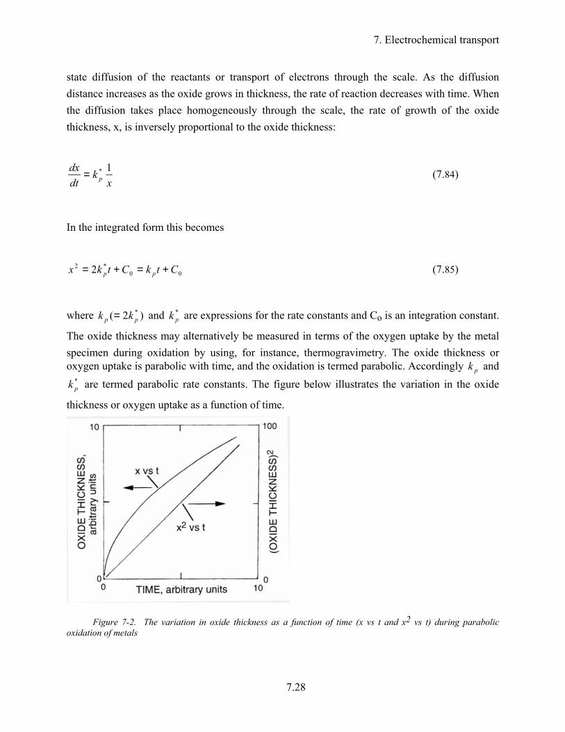
state diffusion of the reactants or transport of electrons through the scale. As the diffusion distance increases as the oxide grows in thickness, the rate of reaction decreases with time. When the diffusion takes place homogeneously through the scale, the rate of growth of the oxide thickness, x, is inversely proportional to the oxide thickness:

xk

dtdx

p1*= (7.84)

In the integrated form this becomes

00*2 2 CtkCtkx pp +=+= (7.85)

where )2( *pp kk = and *

pk are expressions for the rate constants and Co is an integration constant.

The oxide thickness may alternatively be measured in terms of the oxygen uptake by the metal specimen during oxidation by using, for instance, thermogravimetry. The oxide thickness or oxygen uptake is parabolic with time, and the oxidation is termed parabolic. Accordingly pk and

*pk are termed parabolic rate constants. The figure below illustrates the variation in the oxide

thickness or oxygen uptake as a function of time.

Figure 7-2. The variation in oxide thickness as a function of time (x vs t and x2 vs t) during parabolic oxidation of metals


7.29

Carl Wagner developed the theory for parabolic oxidation assuming that the reaction is governed by lattice diffusion of the reacting ions (metal and oxygen ions) or transport of electrons. The important aspect of the Wagner oxidation theory is that the parabolic rate constant is expressed in terms of independently measurable properties, i.e. the electronic and ionic conductivity of the oxide or alternatively in terms of the self-diffusion coefficients of the reacting ions. This thus provides an interpretation of the reaction mechanism and a theoretical basis for changing and improving the oxidation resistance of metals and alloys. The Wagner theory has been one of the most important contributions to our understanding of the high temperature oxidation of metals.

The basic assumption of the theory is that the lattice diffusion of the reacting ions or the transport of electrons through the dense scale is rate-determining for the overall reaction. Lattice diffusion is assumed to take place because of the presence of point defects, and the migrating species may alternatively be considered to constitute lattice and electronic defects. Wagner further assumed that ions and electrons migrate independently of each other and that local equilibria exist within the oxide. Such transport processes through a dense, single-phase scale growing by lattice diffusion is illustrated in the figure below. One part (a) illustrates the transport of metal and oxygen ions and electrons, while the other (b) illustrates the transport processes when the predominant diffusion processes involve metal vacancies and interstitials.

Figure 7-3. Transport processes during growth of a dense, single phase scale growing by lattice diffusion. a) transport processes illustrated by transport of reacting ions, b) transport processes illustrated by transport of diffusion of important point defects (in this case assumed to be metal vacancies and interstitials).


7.30

As diffusion through the scale is rate-determining, reactions at the phase boundaries are considered to be rapid, and it is assumed that thermodynamic equilibria are established between the oxide and oxygen gas at the oxide/oxygen interface and between the metal and the oxide at the metal/oxide interface.

The overall "driving energy" of the reaction is the Gibbs free energy change associated with the formation of the oxide, e.g. MaOb, from the metal M and the oxygen gas. Correspondingly, a gradient in the partial pressure (activity) of oxygen exists across the scale from the partial pressure of oxygen in the ambient atmosphere at the outer surface to the partial pressure of oxygen at the metal/oxide interface. The latter partial pressure is the decomposition pressure of the oxide in equilibrium with its metal.

The main driving force for the transport through the plane is the chemical potential gradient. But when one considers the transport of the reacting ions and of the electrons through the scale, it may also be noted that the mobilities of the cations, anions and electrons are not equal. Because of this difference, a separation of charges takes place in a growing scale. This creates a space charge (diffusion potential) that opposes a further separation of charges, and a stationary state is reached for which no net electric current flows through the scale. In describing the transport of ions and electrons through the scale, it is thus necessary to take into account both the transport due to the gradient of the chemical potential and that due to the gradient of the electrical potential, i.e. the electrochemical potential gradient. Thus, the treatment of the transport through the oxide scale is identical to that done earlier for electrochemical transport through a mixed conducting oxide.

The net ionic current is from earlier given by

dxd

edxd

ezi Oionan

an

ionion

−=−=

2

2ησησ

(7.86)

and the electronic current is given by

dxd

edxd

ei elelelel

elησησ

=−

−=1

(7.87)


7.31

As no net current flows through the scale during the scale growth, then itot = iion + iel = 0. By solving this system in the usual manner (solving for the electrical potential gradient, inserting into the expression for the ionic current density and inserting the equilibrium condition between oxygen ions, oxygen molecules and electrons) we obtain

dxpd

ekTt

dxd

et

i OeliongOelionion

22ln

44)( σµσ

== (7.88)

The rate of oxygen ions reacting per unit area is obtained by dividing the ionic current density by the charge of the oxygen ions. Moreover, the rate dn/dt of oxide molecular units MaOb formed per unit area is obtained by further division by b:

dxpd

bekTt

dxd

bet

ebi

dtdn

bdtdn OeliongOelionionO 22

ln882

12

)(2

σµσ−=−=

−== (7.89)

Similar to the integrations we have done earlier over the thickness of the oxide, we now integrate over the instantaneous thickness ∆x and from the ambient oxygen pressure, 0

2Op , to the partial

pressure at the metal/oxide interface, iOp

2. The growth rate dn

dt then takes the form

∆x p dtσ

bekT

dtdn

Oelion1ln

8

o2O

i2O

2

p

p2

= ∫ (7.90)

We have chosen to organize the equation and direction of integration such that the rate is positive if 0

2Op > iOp

2. In general the directionalities and signs of the fluxes and processes that go on pose

a problem for us. One may most often neglect this issue because the output, namely growth (increase in amount of oxide or thickness of scale) is intuitively positive. However, it may not be just that easy, since there is nothing preventing scale reduction (reverse of growth) if the outer oxygen partial pressure is smaller than the activity at the metal/oxide.

Many readers will probably wonder about another small apparent problem: We integrate over the scale to take into account the steady state condition, namely that the fluxes are constant throughout the scale. Still, the scale grows, so how can it be steady state? The answer is that it is


7.32

steady state (constant fluxes) for that moment of time with that instantaneous thickness of the scale. So our integration is for a given moment in time. At another moment the integration will give a different flux.

The expression in the parentheses,

∫o

2O

i2O

2

p

p2 ln

8 Oelion p dtσbe

kT , can be considered to be one

form of the parabolic rate constant and is in the following written kt:

∆xk

dtdn

t1= (7.91)

kt thus represents a time-independent coefficient, while the flux and thickness of the scale vary according to the parabolic relation above.

As written in this form dndt is expressed in number of molecular units of MaOb per cm2sec

and ∆x in cm. The derivation of Wagner's equation that we here have done for growth of oxide scales, may be applied to many other gas-metal reactions.

It may be noted that although the total particle current is equal to the rate of growth of the scale, the rate-determining process may either be diffusion of ions or transport of electrons depending on the properties of the scales. If the scale is an electronic conductor, tel ≈ 1, the diffusion of the reacting ions through the scale is rate-determining, while the transport of electrons through the scales is rate-determining if the scale is an ionic conductor, tion ≈ 1. The oxygen pressure dependence of the reaction will depend on whether the scale is an ionic or electronic conductor and in the latter case on the type of nonstoichiometry that prevails in the oxide scale.

In our derivation, the growth rate is proportional to σiontel = σtottiontel = (σan + σcat) tel. However, the conductivity of the metal and oxygen ions in MaOb can be expressed in terms of the self-diffusion coefficients of the metal and oxygen ions in MaOb through the Nernst -Einstein relation (zi2e2Dici = kT σi). Let us insert this relationship in Eq.7.89 and assume that the oxide is an electronic conductor (tel ≈ 1). Let us furthermore take into account that concentrations of metal ions (cations), cM, and oxygen ions, cO, in an oxide MaOb with relatively small deviation from stoichiometry are related through cM/cO = a/b = |zan|/zcat. The expressions for the flux through the growing scale (expressed in terms of the number of MaOb units per cm2sec.) and for kt then become


7.33

dxpd

DDz

bc

dxpd

DDzz

bzc

dtdn O

OMcatOO

OMan

catanO 22ln

)2

(2

ln)(

8

2

+−=+−= (7.92)

∆xk

∆xpdDD

zb

c

dtdn

tOOMcat 11ln)2

(2 2

o2O

i2O

p

p

0 =

+= ∫ (7.93)

cO denotes the number of oxygen ions in MaOb per cm3 and DM and DO are respectively the self-diffusion coefficients of the metal and oxygen ions in MaOb. It should be noted that DM and DO are the self-diffusion coefficients for random diffusion of the respective ions.

In Eqs.7.92 and 7.93, kt represents the rate of formation of MaOb units per cm2 per second for an MaOb scale of thickness 1 cm. One may as said before alternatively express the parabolic rate constant in terms of the rate of growth of the oxide thickness

xk

dtdx

p1*= (7.94)

The dimensions of k*p are then cm2sec-1, and Eq.7.93 then takes the form

∆xk

∆xpdDD

z

dtdn

cb

dtdx

pOOMcat 11ln)2

(21 *

p

p02

o2O

i2O

=

+== ∫ (7.95)

Growth of metal-deficient Ma-yOb on M

Let us make use of Eq. 7.95 to illustrate the temperature and oxygen pressure dependence of the parabolic rate constant. Consider the growth of the metal deficient oxide Ma-yOb on high purity M. Let us assume that the predominant defects throughout the entire scale are metal

vacancies with an effective charge α, i.e. Vα'M . Let us further assume that the metal ion diffusion

is much faster than the oxygen diffusion, i.e. DM >> DO. Eq. 7.95 then reduces to


7.34

∆xk

∆xpdD

zdtdx

pOMcat 11ln4

*p

p2

o2O

i2O

=

= ∫ (7.96)

In order to integrate this we need to analyse the defect structure of the oxide. The formation of the metal vacancies may be written as

xOM O

abhvgO

ab ++= •αα /

2 )(2

(7.97)

If other defects may be neglected and the electroneutrality condition is given by α[Vα'M ] = p, the

concentration of metal vacancies is given by

ab

OVM pKvM

2/1/2/][ α

ααα =+ (7.98)

where /αMV

K is the equilibrium constant for the formation of the metal vacancies (Eq. 7.97) and

][ /αMv denotes the fraction of the metal ion sites that are vacant. On the basis of this relation,

2ln Opd may be written

][ln)1(2ln /2

ααMO vd

bapd += (7.99)

When this expression for 2

ln Opd is introduced in Eq.7.96 , the expression for k*p becomes

][][)1( i/o/*/

αααα MMvp vvDkM

−+= (7.100)

If the concentration of metal vacancies at the oxide/oxygen interface is much larger than at the metal/oxide interface, i.e. i/o/ ][][ αα

MM vv >> then


7.35

oMMvp DvDk

M)1(][)1( o/*

/ +=+= αα αα (7.101)

where o/ ][/α

α MvoM vDD

M= is the self-diffusion coefficient of the metal ions in Ma-yOb at the

oxide/oxygen interface. Thus under these conditions the parabolic rate constant and the self-diffusion coefficient of M in Ma-yOb has the same temperature and oxygen pressure dependences.

Growth of oxygen-deficient MaOb-y on M

The same procedure may be used to derive the parabolic rate constant for the growth of oxygen deficient MaOb-y on M. let us assume that the oxygen vacancies have α charge α, i.e.

Vα.O , and the formation of the oxygen vacancies may then be written

OO = Vα.O + αe' + 12 O2 (7.102)

If DO>>DM and (piO2 <<p

oO2 ) then k

*p becomes

)1(21

2)()1()1(][)1( 0i* +

−

• +=+=+= • αα ααα α i

OOiOOvp pDDvDk

O (7.103)

where •αOvD is the self-diffusion coefficient of the oxygen vacancies, i][ •α

Ov the concentration of

oxygen vacancies and DOi the self-diffusion coefficient of oxygen in MaOb-y at the metal/oxide

interface. DO0 is the oxygen self-diffusion coefficient at 1 atm. O2, and piO2 is the oxygen

activity at the metal/oxide interface. For this case the parabolic rate constant is independent of the ambient oxygen pressure, and the temperature dependence is given by that of the oxygen self-diffusion coefficient in MaOb-y at the metal/oxide interface. In this respect it may be further noted that the oxygen self-diffusion coefficient at the metal/oxide interface is given by that the product of the self-diffusion coefficient of oxygen at constant oxygen pressure (at 1 atm O2) and

(piO2 )-1/2(α+1) , i.e. DOi = DO0 (p

iO2 )-1/2(α+1) . In these terms the activation energy of the

parabolic rate constant is under these conditions given by the activation energy associated with


7.36

DO0 and the enthalpy term associated with (piO2 )-1/2(α+1) . Similar treatments may be given for

oxide scales growing by interstitial metals ions or interstitial oxygen ions.

Scales with ionic conductivity predominant.

Most oxides encountered in high temperature oxidation of metals are electronic conductors. In the literature there are no examples of high temperature metal-oxygen reactions involving conventional metals or alloys with essentially pure ionic conductivity over the entire existence range of the oxide. Such type of reactions are, however, found in metal-halogen reactions, e.g. Ag+Br2 to form AgBr. The same treatment as given above may be applied to reactions involving formation of ionically conducting scales, and the important feature of these reactions is that it is the electronic transport through the scale that is rate-determining.

Varying defect structure situations through the scale.

In the preceding examples it has been assumed that the same defect structure prevails throughout the entire scale from the scale/gas to the metal oxide interfaces. This is an oversimplified model for many systems. The charge on the defects, or even the predominant defects may change with changing oxygen activity. Furthermore, the presence of impurities and dopants may significantly affect the defect structure situation. Thus, following the discussion in Ch.4 one part of the scale may possibly have intrinsic properties and another part extrinsic properties. As part of such behaviour one part of the scale may have significant ionic conductivity while the rest has electronic conductivity.

In the presence of water vapour, hydrogen defects may affect the diffusional behaviour in growing oxide scales in many different ways.

Diffusion–limited creep

General terms and mechanisms

Creep represents plastic deformation of solids under an applied stress. At high temperatures and under constant applied stress, a steady state is reached (secondary creep stage) where the rate of deformation remains constant. The steady state creep rates of crystalline solids can be expressed by the equation


7.37

ε = f(s) σnstr exp( -Q/RT) (7.104)

where f(s) is a function which is dependent upon the structure, σstr is the applied stress, n is a constant and Q the activation energy.

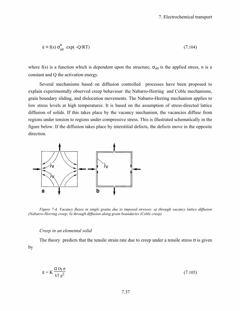
Several mechanisms based on diffusion controlled processes have been proposed to explain experimentally observed creep behaviour: the Nabarro-Herring and Coble mechanisms, grain boundary sliding, and dislocation movements. The Nabarro-Herring mechanism applies to low stress levels at high temperatures. It is based on the assumption of stress-directed lattice diffusion of solids. If this takes place by the vacancy mechanism, the vacancies diffuse from regions under tension to regions under compressive stress. This is illustrated schematically in the figure below. If the diffusion takes place by interstitial defects, the defects move in the opposite direction.

Figure 7-4. Vacancy fluxes in single grains due to imposed stresses: a) through vacancy lattice diffusion (Nabarro-Herring creep; b) through diffusion along grain boundaries (Coble creep)

Creep in an elemental solid

The theory predicts that the tensile strain rate due to creep under a tensile stress σ is given by

ε = K Ω Dl σ

kT g2 (7.105)


7.38

where K is a geometrical constant, Ω is the atomic volume, Dl is the lattice self-diffusion coefficient, g is the length of the diffusion path (i.e. the average grain size), k is the Boltzmann constant and T the absolute temperature. The Nabarro-Herring creep rate is thus proportional to the stress and the activation energy is equal to that for the self-diffusion.

In polycrystalline solids the defects (or atoms) can migrate by both lattice and grain boundary diffusion and as discussed in Chapter 5 the effective diffusion coefficient may be written

gD3

D gbeff

δ+= lD (7.106)

If this value for Deff is substituted for the lattice diffusion coefficient, Dl, the creep rate becomes

)D g

3 + (D g kTsW gbl2

δε K= (7.107)

If lattice diffusion is negligible compared with grain boundary diffusion, this reduces to

ε = K 3Ω σkT g3 δDgb (7.108)

This mechanism was first proposed by Coble, and it is illustrated schematically in Fig.7.8b. Also in this case the strain rate is proportional to the stress. Both the Nabarro-Herring and Coble mechanisms are favoured by small grain sizes.

Creep in compounds

In a compound, e.g. an oxide MaOb, the creep process is more complicated in that both metal and oxygen atoms (or ions) must migrate in order to conserve electroneutrality and


7.39

maintain local composition of the oxide. Thus the fluxes of the metal and oxygen ions are coupled, and one must consider the flow of "molecular units" of MaOb. The molecular diffusion coefficient Dmol is a composite value of the self-diffusion of the metal and oxygen ions and is given by

Dmol = DM DO

aDO + bDM (7.109)

In the expressions for the creep rates, the molecular volume must be substituted for the atomic volume:

Ωmol = aΩM + bΩO (7.110)

The value of Dmol may be expressed either in terms of the lattice self-diffusion coefficients for metal and oxygen ions for Nabarro-Herring creep or in terms of Deff for creep taking place by simultaneous lattice and grain boundary diffusion.

From Eq. 7.109 it is seen that the creep rate is governed by the diffusion of the slower moving species. Thus, if metal ions diffuse much faster than the oxygen ions, DM>>DO, then

Dmol = 1b DO (7.111)

and accordingly the creep rate is determined by the diffusion of oxygen atoms in MaOb. A meaningful interpretation of the creep behaviour in terms of the diffusion processes thus requires knowledge of the self-diffusion of both components in the binary compound.

In addition to the above models other creep mechanism have been advanced based on dislocation movements in the material.


7.40

Sintering

Stages of the sintering process

Sintering is the process whereby powders and small particles agglomerate and grow together to form a continuous polycrystalline body. As a rule of thumb the material must be heated to 2/3 of the melting temperature to achieve considerable sintering.

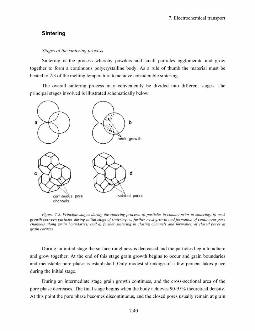
The overall sintering process may conveniently be divided into different stages. The principal stages involved is illustrated schematically below.

Figure 7-5. Principle stages during the sintering process: a) particles in contact prior to sintering; b) neck growth between particles during initial stage of sintering; c) further neck growth and formation of continuous pore channels along grain boundaries; and d) further sintering in closing channels and formation of closed pores at grain corners.

During an initial stage the surface roughness is decreased and the particles begin to adhere and grow together. At the end of this stage grain growth begins to occur and grain boundaries and metastable pore phase is established. Only modest shrinkage of a few percent takes place during the initial stage.

During an intermediate stage grain growth continues, and the cross-sectional area of the pore phase decreases. The final stage begins when the body achieves 90-95% theoretical density. At this point the pore phase becomes discontinuous, and the closed pores usually remain at grain


7.41

boundaries. The final stage may involve complete removal of the remaining pores, leading to a completely dense material. Alternatively, it may involve discontinuous growth of the large grains at the expense of the small ones, and closed pores may as a consequence be isolated inside the grains. If the latter process occurs, complete densification becomes extremely difficult.

Driving force for sintering

During sintering, as for other spontaneous processes, the total free energy of the system decreases. For elemental solids and homogeneous compounds the only free energy change involved in sintering is that of the surface free energy or surface tension, γ, of the particles.

Any surface atom or molecule is subjected to a resultant inward attraction because of the unsaturated chemical bonds at the surface. The surface therefore tends to contract to the smallest possible area. In the case of a spherical particle with radius r, the interior is subjected to an excess force of πr2p, where p is the pressure. This is counteracted by the surface tension acting along the circumference: 2πrγ. When equating these opposing forces, the pressure is given by

p = 2πrγπr2

= 2γr (7.112)

From this it is seen that the vapour pressure of a sphere is larger the smaller the radius and as a result a large sphere will grow at the expense of a neighbouring small sphere. This type of grain growth in polycrystalline solids is termed Ostwald's law. Similarly the vapour pressure of convex surfaces is larger than the vapour pressure of a concave surface and as a result surface roughness of particles is reduced during the initial stage of sintering.

Transport processes during sintering

As for creep, sintering of oxides implies that molecular units of the oxide are transported from areas from high to low surface free energies, e.g. from convex to concave surfaces. Generally it is concluded that transport of the slower moving species determines the overall sintering rate. Thus, in a binary oxide where oxygen ions diffuse much more slowly than the metal ions, it is generally to be expected that the sintering rate is determined by the transport, e.g. lattice or grain boundary diffusion of oxygen.


7.42

Sintering governed by lattice diffusion will be dependent upon the concentration of point defects in oxides. Accordingly, sintering rates of an oxide can be optimised by close control of impurities or dopants and the ambient partial pressures of oxygen and of water vapour in cases where proton defects affect the defect structure of the oxide.

Oxides with additional transport of protons

If an oxidic material conducts protons in addition to oxygen ions and electrons we need to introduce electrochemical equilibria between neutral and charged species of both oxygen and hydrogen:

O2e4+(g)O 22

−− = (7.113)

e+H2(g)H 2−+= 2 (7.114)

for which equilibria can be expressed by

O2d

e4d+Od 2

2(g) −− =µµ (7.115)

ed+

H2dHd (g)

2−+= µµµ 2 (7.116)

We insert these into the flux equations for the species and utilise that the sum of all transport numbers equals unity. We furthermore use that dµ = kTdlna • kTdlnp, where a and p are activity and partial pressure, respectively, and obtain

dxd

e1+

dxpd

2ekTt-

dxpd

4ekTt+i-=

dxd eHHOO

tot

tot 2+

2-2 µ

σφ lnln

(7.117)


7.43

This can now be integrated to obtain the voltage of a cell, or inserted into a flux equation of a species of interest in the usual manner. We now have a system with two chemical driving forces for electrochemical transport; that of oxygen activity and that of hydrogen activity.

Other cases

We have in the present version of the treatment of electrochemical transport omitted many cases. These include a more full coverage of proton transport in oxides and transport by other hydrogen species and other foreign species. Moreover, we have left out the case of solid-solid reactions. Also, creep and sintering were given more phenomenological than defect-chemical treatments.

We have throughout assumed isothermal conditions. If we instead of (or in addition to) chemical driving forces considered a temperature gradient, our integrations over membranes would have been from one temperature to another. The voltage we would have obtained would be the thermoelectric voltage. It has several contributions, but in general it is related to the transport numbers and the gradients in concentrations of defects. The variations of concentration is in turn given by the entropy of the defects.

More on these themes will be included in future updates.


7.44

electrochemical potential - uio.no · 7. electrochemical transport 7.2 flux equations – wagner...

Documents