electricity capacity assessment report 2014
TRANSCRIPT

Ofgem/Ofgem E-Serve 9 Millbank, London SW1P 3GE www.ofgem.gov.uk
Electricity Capacity Assessment Report 2014
Annual report
Publication date: 30 June 2014 Contact: Christos Kolokathis, Economist/Analyst
Team: Energy Market Outlook
Tel: 020 7901 7000
Email: [email protected]
Overview
This document is Ofgem’s annual report to the Secretary of State assessing the risks to electricity
security of supply in Great Britain for the next five winters.
Our assessment is based on data from National Grid accompanied by our own analysis. It suggests
that, absent new measures that have been introduced, the risks to the security of our electricity
supply over the next five winters would be broadly consistent with those in last year’s report.
Margins are expected to fall over the next two winters as older power stations close, before
improving in the later years of our analysis.
Unlike last year, we now have new measures that were introduced by Ofgem, National Grid and the
government. The New Balancing Services and the Capacity Market mean that the risk of disruption
to customer supplies in the coming winters has reduced compared to last year’s report.

Electricity Capacity Assessment Report 2014
2
Context
Ofgem's principal objective is to protect the interests of existing and future energy consumers.
This includes their interests in the reduction of greenhouse gases and in in secure supplies of
electricity and gas. In this document the Gas and Electricity Markets Authority is referred to as
“the Authority” or as “Ofgem”.
We first highlighted concerns over security of supply in the 2010 Project Discovery. Following this,
we were given a new requirement1 to provide the Secretary of State with a report assessing
plausible electricity capacity margins and the risk to security of supply associated with each
alternative. This Electricity Capacity Assessment report has to be delivered to the Secretary of
State by 1 September each year. It is intended to inform government and Ofgem decisions on
electricity security of supply.
Producing these reports required the development of a model to assess the risks to electricity
security of supply. This model was developed in 2012 and amended in 2013. For the 2014 report,
we have used the 2013 model with minor changes and the latest data. These changes are
discussed in the 2014 methodology consultation and decision documents.
The Electricity Act 1989 allows us to delegate the modelling to a transmission licence holder. We
delegated construction of the model to National Grid Electricity Transmission plc (National Grid).
Associated documents
All Capacity Assessment documents can be found on:
www.ofgem.gov.uk//electricity/wholesale-market/electricity-security-supply
The most recent documents can be found below:
Electricity Capacity Assessment 2014: decision on methodology
Electricity Capacity Assessment 2014: Consultation on methodology Electricity Capacity Assessment Report 2013
1 Section 47ZA of the Electricity Act 1989, as amended by the Energy Act 2011.

Electricity Capacity Assessment Report 2014
3
Contents
Executive Summary ......................................................................................................... 4
1. Key results .................................................................................................................. 7 National Grid’s scenarios .......................................................................................................................... 10 Sensitivity analysis ................................................................................................................................... 15
2. Methodology .............................................................................................................. 26
3. Wider range of sensitivities ....................................................................................... 31
Appendices .................................................................................................................... 43
Appendix 1 – Detailed results tables ............................................................................. 44
Appendix 2 - Glossary .................................................................................................... 55
Electricity Capacity Assessment Report 2014
4
Executive Summary
This report assesses the risks to the security of Britain’s electricity supply over the winters
2014/15 to 2018/19. Our updated analysis shows that, absent new measures introduced by the
Government, Ofgem and National Grid, the outlook for security of supply would be broadly the
same as seen in our 2013 report.
Since last year’s report, two measures have been introduced to reduce the risk to customer
disconnections: we have approved new tools (the New Balancing Services) that National Grid can
use to help balance the system when margins are tight. The Government has also set out firm
plans to introduce the Capacity Market to reduce risks to security of supply in the medium term
and beyond. In addition, the Government has set the level of resource adequacy for the electricity
system in Great Britain (GB), the Reliability Standard2.
Methodology
Our results are based on National Grid’s forthcoming Future Energy Scenarios (FES) over the next
five winters. These four scenarios cover different views of the electricity market, taking into
account changes in the outlook since last year.
Even during the relatively short time horizon of this analysis, there is significant uncertainty over
the security of supply outlook. We assess these uncertainties using sensitivity analysis around
National Grid’s scenarios. These sensitivities illustrate only changes in one variable at a time and
do not capture potential mitigating effects, for example the supply side reacting to higher demand
projections.
Our results show the range of risks implied by National Grid’s FES and a broader range of risks
resulting from the sensitivities. This broader range presents Ofgem’s view of the most likely
outcomes but is not exhaustive.3
Our results
As in our Capacity Assessment 2013, we expect a reduction in generation margins over the next
two winters, with de-rated margins dropping to their lowest level in 2015/16 as a result of a
reduction in supplies from conventional generation. There has been a sharp reduction in demand
since last year, which National Grid believes comes from energy efficiency measures, an increase
in generation connected to distribution networks, and demand reduction by the industrial and
commercial sectors at times of peak demand. But this has been offset by a greater reduction in
available electricity supply than previously expected.
There are a number of measures used in relation to security of supply. They include de-rated
margins; loss of load expectation; and risk of customer disconnections. Expected changes to de-
rated margins or loss of load expectation in the next few years do not necessarily entail an
increase in the risk of customer disconnections. Our analysis shows that, due to the introduction
of the New Balancing Services, the expected risk of customer disconnections will remain in the
range estimated for recent years. De-rated margins are expected to improve later in the decade
as available supplies increase.
2 The Reliability Standard is set at 3 hours loss of load expectation per year. This report does not provide information on how much capacity is needed to reach the Reliability Standard, nor how much capacity to procure for any of these tools. National Grid and DECC will decide on procurement volumes for New Balancing Services and the Capacity Market respectively. 3 Wider sensitivities are modelled and set out in Chapter 3 of the report. It may be appropriate to use a wider range of uncertainties when making procurement decisions relating to New Balancing Services or the Capacity Market, for example, how risks could change in a cold winter.

Electricity Capacity Assessment Report 2014
5
De-rated margins
We use de-rated margins to show the average excess of supply over peak demand under average
winter conditions. This is based on the amount of electricity the market could deliver over the next
five winters under normal operation of the system. It does not directly represent the risk of
customers being disconnected.
In general, National Grid’s scenarios (the central range in the graph below) assume that demand
will continue to decline in the next five winters, but that this is cancelled out by deteriorations on
the supply side as a result of further plant closures and mothballing. National Grid projects that
the supply outlook will continue to deteriorate before improving after 2015/16. All of its scenarios
assume that imports of electricity via the interconnectors will be balanced by exports for all years
of the analysis.4 National Grid’s scenarios show that the de-rated margins will drop until 2015/16,
reaching a minimum of around 3%, and then recover.
Our sensitivity analysis shows that the de-rated margins could vary between around 2% and 8%
in 2015/16. They could drop to around 2% if, for example, demand was higher than projected by
National Grid. Fewer imports from mainland Europe and further plant closures or mothballs could
also lead to the same outcome. If electricity from the Continent was flowing at the maximum
available capacity, the risks to security of supply would be significantly lower, with de-rated
margins around 8%. Fewer plant closures or lower demand in the future could have a similar
impact.
De-rated margins
Loss of Load Expectation
The de-rated margins are a useful way to illustrate trends in the market, but this measure has
limitations. We therefore also use the measure of loss of load expectation. This is the average
number of hours in a year where we expect National Grid may need to take action that goes
beyond normal market operations. Importantly, this still does not represent the likelihood of
customer disconnections. Controlled disconnections of customers – typically industrial and
commercial sites before households - would only take place if a large deficit were to occur. This is
because the System Operator is usually able to manage supply shortfalls up to a certain level with
little or no impact on customers, through using New Balancing Services or other mitigating
measures such as voltage control.
4 We include a wider range in our sensitivity analysis to reflect uncertainty.
0%
2%
4%
6%
8%
10%
12%
14%
16%
2014/15 2015/16 2016/17 2017/18 2018/19
De
-rat
ed
cap
acit
y m
argi
n [
%]
Pessimistic sensitivity range FES range Optimistic sensitivity range
The New Balancing Services in the short-term and Capacity Market from the medium-term will reduce the risk to customer disconnections
Electricity Capacity Assessment Report 2014
6
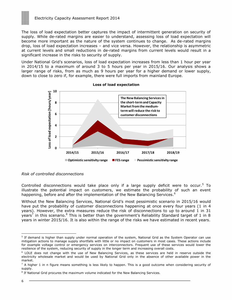
The loss of load expectation better captures the impact of intermittent generation on security of
supply. While de-rated margins are easier to understand, assessing loss of load expectation will
become more important as the nature of the system continues to change. As de-rated margins
drop, loss of load expectation increases – and vice versa. However, the relationship is asymmetric
at current levels and small reductions in de-rated margins from current levels would result in a
significant increase in the risks to security of supply.
Under National Grid’s scenarios, loss of load expectation increases from less than 1 hour per year
in 2014/15 to a maximum of around 3 to 5 hours per year in 2015/16. Our analysis shows a
larger range of risks, from as much as 9 hours per year for a higher demand or lower supply,
down to close to zero if, for example, there were full imports from mainland Europe.
Loss of load expectation
Risk of controlled disconnections
Controlled disconnections would take place only if a large supply deficit were to occur.5 To
illustrate the potential impact on customers, we estimate the probability of such an event
happening, before and after the implementation of the New Balancing Services.6
Without the New Balancing Services, National Grid’s most pessimistic scenario in 2015/16 would
have put the probability of customer disconnections happening at once every four years (1 in 4
years). However, the extra measures reduce the risk of disconnections to up to around 1 in 31
years7 in this scenario.8 This is better than the government’s Reliability Standard target of 1 in 8
years in winter 2015/16. It is also within the range of the risks we have estimated in recent years.
5 If demand is higher than supply under normal operation of the system, National Grid as the System Operator can use mitigation actions to manage supply shortfalls with little or no impact on customers in most cases. These actions include for example voltage control or emergency services on interconnectors. Frequent use of these services would lower the resilience of the system, reducing security of supply in the longer term and increasing overall costs. 6 LOLE does not change with the use of New Balancing Services, as these services are held in reserve outside the electricity wholesale market and would be used by National Grid only in the absence of other available power in the market. 7 A higher 1 in n figure means something is less likely to happen. This is a good outcome when considering security of supply. 8 If National Grid procures the maximum volume indicated for the New Balancing Services.
0
2
4
6
8
10
2014/15 2015/16 2016/17 2017/18 2018/19
Loss
of l
oad
exp
ect
atio
n [h
ou
rs/y
ear
]
Optimistic sensitivity range FES range Pessimistic sensitivity range
The New Balancing Services in the short-term and Capacity Market from the medium-term will reduce the risk to customer disconnections
Electricity Capacity Assessment Report 2014
7
1. Key results
1.1. This report fulfils the Authority’s obligation9 to provide the Secretary of State with an
annual report assessing the risks to the security of Great Britain’s (GB) electricity supply
from 2014/15 to 2018/19. The main purpose of this report is to illustrate the levels of
security that could be delivered by the market alone over this period and inform Ofgem’s
and the government’s decisions on security of supply. We also analyse the potential impact
of the new balancing services introduced by National Grid, Ofgem and the Department of
Energy and Climate Change (DECC) on the risk to customer disconnections.
1.2. Since last year’s report, National Grid, Ofgem and DECC have introduced two measures to
address the risks to security of electricity supply. We have approved new tools (the New
Balancing Services) that National Grid can use to balance the system if margins tighten.
The government has also confirmed its intention to introduce the Capacity Market10 to
reduce risks to security of supply in the medium term and beyond. We expect the new
balancing services to mitigate the consequences of the tightening margins until the
Capacity Market comes into effect in 2018/19.11
1.3. Our 2014 assessment shows that, in the absence of the measures taken by National Grid,
Ofgem and the Government, the outlook for security of supply over the next five winters is
largely similar to the one we presented in our 2013 report.12 We expect a reduction in de-
rated margins over the next two winters, with de-rated margins dropping to their lowest
level in 2015/16, driven by a reduction of electricity supplies from conventional generation.
De-rated margins are then expected to improve as new conventional plant comes online
and some mothballed plant returns to the market.
1.4. Our results are based on National Grid’s forthcoming Future Energy Scenarios (FES).13
These four scenarios cover different views of the electricity market over the next five
winters, taking into account changes in the outlook since last year.
1.5. There is a high level of uncertainty around the supply and demand outlook for this period
which is not fully captured by National Grid’s scenarios. We have undertaken sensitivity
analysis to assess the risks associated with these uncertainties.
9 As set out in section 47ZA of the Electricity Act 1989. 10 The Capacity Market works by offering all capacity providers (new and existing power stations, electricity storage and capacity provided by demand side response) a steady, predictable revenue stream on which they can base their future investments. For more information see: www.gov.uk/government/policies/maintaining-uk-energy-security--2/supporting-pages/electricity-market-reform. 11 National Grid has announced its intention to procure new balancing services for the coming two winters. The ongoing need for these services after 2015/16 will be reviewed early in 2016 via an industry consultation process. For more information see:
www.nationalgrid.com/NR/rdonlyres/D63DC28A-ACC9-496E-A39C-1682CF25EE08/63428/VolumeRequirementOpenLetter.pdf. 12 Our assessment considers policies that are already in place, ie in the absence for example of the new balancing services, Capacity Market or the Electricity Balancing Cash-Out Reform. 13 National Grid will publish the forthcoming FES on 10 July 2014. The publication will be available here: www.nationalgrid.com/fes.

Electricity Capacity Assessment Report 2014
8
1.6. In this chapter we present the range of risks implied by National Grid’s FES and a broader
range of risks resulting from the sensitivities described above. This range is our view of the
risks associated with the most likely outcomes for supply and demand. The range is implied
by independent changes to the key assumptions of demand, supply and interconnector
flows and presents a central view of the risks. A wider range of sensitivities is presented in
Chapter 3. Below we present the key figures from our analysis14:
De-rated margins: is the average excess of available generation over peak demand.
These could vary between around 2% and 8% in 2015/16. We then expect them to
increase to a minimum of around 3% for the pessimistic range and above
approximately 8% for the optimistic range, for the rest of the analysis period.
Loss of load expectation (LOLE): is the average expected number of hours per year in
which supply is expected to be lower than demand under normal operation of the
system. As de-rated margins drop in the mid-decade, the LOLE is projected to
increase to a maximum of around 9 hours in 2015/16, before it drops to a maximum
of around 3 hours for the last three winters of the analysis. For the optimistic range
the LOLE remains at approximately zero levels for the entire period.
Likelihood of controlled disconnections: shows the probability of a large shortfall
occurring that would require controlled disconnections of customers – which are
expected to affect industrial and commercial sites before households. We estimate the
likelihood of controlled disconnections with a 1 in n years metric, including the
potential impact of the new balancing services. Without the new balancing services
the likelihood of controlled disconnections would vary between about 1 in 8 to 1 in 4
years in 2015/16 for National Grid’s FES. However, if National Grid procured the
maximum volume of new balancing services it has indicated for 2015/16, the
additional measures would reduce the risk of disconnections to up to around 1 in 73
to 1 in 31 years for the FES.
1.7. More extreme changes in one variable or a combination of changes in different variables
would result in a wider range of risk. Chapter 3 of this report presents some of these more
extreme cases. These outcomes are less likely but still possible and relevant to the analysis
of security of supply.
1.8. The rest of this chapter is structured as follows: we first provide a short description of the
methodology we have used in this assessment, followed by the key assumptions in National
Grid’s FES and the risks associated with these. We then discuss the assumptions and
results of the sensitivity analysis around the key uncertainties for our central range. Finally
we present the potential impacts to customers before and after the introduction of new
balancing services and provide historical context to the risks to security of supply.
1.9. The remainder of the Electricity Capacity Assessment Report 2014 is structured as follows:
Chapter 2 presents a brief description of the methodology used for our analysis.
14 For more details see the Sensitivity Analysis section of this Chapter.

Electricity Capacity Assessment Report 2014
9
Chapter 3 presents the results of a wider sensitivity analysis we have considered for
this report.
Appendix 1 details the numerical results behind the figures presented throughout this
report in table format. Appendix 2 provides a glossary of terms used in this report.
Methodology
1.10. Our assessment is based on National Grid’s forthcoming FES.15 These scenarios provide a
credible and plausible range of potential outcomes, but there are significant uncertainties
around the evolution of the market that make it difficult to accurately assess the risks to
security of supply in the coming years. Key uncertainties include the level of peak demand,
commercial decisions of generators and interconnector flows, among others. Our sensitivity
analysis captures the impact of these uncertainties.
1.11. To calculate the risk indicators we use a probabilistic model. The model captures the
uncertainty due to variable generation, plant faults and demand variations. We also use
sensitivity analysis to account for uncertainties that cannot be given credible probabilities.
These include, for example, uncertainties related to future economic growth and policy
development and their potential impacts on future demand, investment and retirement
decisions and interconnector flows.
1.12. The methodology was designed by Ofgem and National Grid. National Grid developed the
probabilistic model in close collaboration with Ofgem, following consultation with industry16
and academics.17 LCP Consulting validated the probabilistic model.
1.13. We present the de-rated margin which is the average excess of available generation over
peak demand. This is not a good indicator of risk, as it is an average value and provides no
information about the variability around this average value. However, we include it in our
analysis as it is a widely used and easily understood indicator of risks to security of supply.
1.14. We therefore use the probabilistic measure of loss of load expectation (LOLE). The LOLE is
the average expected number of hours per year in which supply is expected to be lower
than demand under normal operation of the system. This means the number of hours per
year when we expect National Grid to have to use mitigation actions, including the use of
the new balancing services. The LOLE is still not a measure of the expected number of
hours in which customers may be disconnected as National Grid is expected to use other
mitigation actions ahead of controlled customer disconnections.
1.15. To illustrate the tangible effects of risk measures for electricity customers we present the 1
in n years metric. This shows the probability of a large shortfall occurring that would
require controlled disconnections of customers – which are expected to involve industrial
and commercial sites before households. It is based on judgments of how the electricity
15 This represents a change from our previous assessments that were based on National Grid’s Gone Green scenario. 16 The methodology was consulted with industry and academics in 2011, 2012 and 2013. The consultation documents,
corresponding responses and decision documents can be found in www.ofgem.gov.uk/electricity/wholesale-market/electricity-security-supply. 17 This year’s academic advisory group consists of Prof. Derek Bunn (London Business School), Prof. Keith Bell (University of Strathclyde), and Dr. Nick Eyre (University of Oxford).
Electricity Capacity Assessment Report 2014
10
system would operate when supply does not meet demand, and the order and size of
mitigation actions taken by National Grid as the System Operator. It is not as accurate as
the LOLE but it allows us to provide a view of the probability of controlled disconnections.
1.16. We also present the expected energy unserved (EEU) and equivalent firm capacity (EFC)
for wind, which are described in Chapter 2.
National Grid’s scenarios
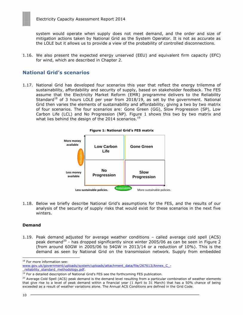
1.17. National Grid has developed four scenarios this year that reflect the energy trilemma of
sustainability, affordability and security of supply, based on stakeholder feedback. The FES
assume that the Electricity Market Reform (EMR) programme delivers to the Reliability
Standard18 of 3 hours LOLE per year from 2018/19, as set by the government. National
Grid then varies the elements of sustainability and affordability, giving a two by two matrix
of four scenarios. The four scenarios are: Gone Green (GG), Slow Progression (SP), Low
Carbon Life (LCL) and No Progression (NP). Figure 1 shows this two by two matrix and
what lies behind the design of the 2014 scenarios.19
Figure 1: National Grid’s FES matrix
1.18. Below we briefly describe National Grid’s assumptions for the FES, and the results of our
analysis of the security of supply risks that would exist for these scenarios in the next five
winters.
Demand
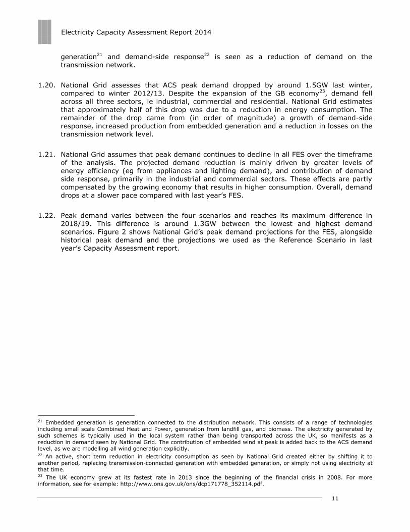
1.19. Peak demand adjusted for average weather conditions – called average cold spell (ACS)
peak demand20 - has dropped significantly since winter 2005/06 as can be seen in Figure 2
(from around 60GW in 2005/06 to 54GW in 2013/14 or a reduction of 10%). This is the
demand as seen by National Grid on the transmission network. Supply from embedded
18 For more information see: www.gov.uk/government/uploads/system/uploads/attachment_data/file/267613/Annex_C_-_reliability_standard_methodology.pdf. 19 For a detailed description of National Grid’s FES see the forthcoming FES publication. 20 Average Cold Spell (ACS) peak demand is the demand level resulting from a particular combination of weather elements that give rise to a level of peak demand within a financial year (1 April to 31 March) that has a 50% chance of being exceeded as a result of weather variations alone. The Annual ACS Conditions are defined in the Grid Code.
More money available
Less money available
More sustainable policies.
Gone Green
Low Carbon
Life
Slow
Progression
No
Progression
Less sustainable policies.
Electricity Capacity Assessment Report 2014
11
generation21 and demand-side response22 is seen as a reduction of demand on the
transmission network.
1.20. National Grid assesses that ACS peak demand dropped by around 1.5GW last winter,
compared to winter 2012/13. Despite the expansion of the GB economy23, demand fell
across all three sectors, ie industrial, commercial and residential. National Grid estimates
that approximately half of this drop was due to a reduction in energy consumption. The
remainder of the drop came from (in order of magnitude) a growth of demand-side
response, increased production from embedded generation and a reduction in losses on the
transmission network level.
1.21. National Grid assumes that peak demand continues to decline in all FES over the timeframe
of the analysis. The projected demand reduction is mainly driven by greater levels of
energy efficiency (eg from appliances and lighting demand), and contribution of demand
side response, primarily in the industrial and commercial sectors. These effects are partly
compensated by the growing economy that results in higher consumption. Overall, demand
drops at a slower pace compared with last year’s FES.
1.22. Peak demand varies between the four scenarios and reaches its maximum difference in
2018/19. This difference is around 1.3GW between the lowest and highest demand
scenarios. Figure 2 shows National Grid’s peak demand projections for the FES, alongside
historical peak demand and the projections we used as the Reference Scenario in last
year’s Capacity Assessment report.
21 Embedded generation is generation connected to the distribution network. This consists of a range of technologies including small scale Combined Heat and Power, generation from landfill gas, and biomass. The electricity generated by such schemes is typically used in the local system rather than being transported across the UK, so manifests as a reduction in demand seen by National Grid. The contribution of embedded wind at peak is added back to the ACS demand level, as we are modelling all wind generation explicitly. 22 An active, short term reduction in electricity consumption as seen by National Grid created either by shifting it to
another period, replacing transmission-connected generation with embedded generation, or simply not using electricity at that time. 23 The UK economy grew at its fastest rate in 2013 since the beginning of the financial crisis in 2008. For more information, see for example: http://www.ons.gov.uk/ons/dcp171778_352114.pdf.
Electricity Capacity Assessment Report 2014
12
Figure 2: National Grid’s ACS peak demand projections in the FES24
Largest infeed loss reserve25
1.23. National Grid reserves power to maintain system frequency within statutory limits in the
event of the loss of the largest generator (the largest infeed loss).26 Its importance is such
that National Grid would curtail demand before using this reserve. The generation capacity
required for this reserve will therefore not be available under normal market operation and
this is reflected within the assumptions of our analysis. We do this by including it as
additional demand in our analysis.
1.24. National Grid estimates that the reserve requirement for the largest infeed loss is 0.9GW
and remains constant throughout our analysis period increasing only when the credible
level of the largest generation loss in a particular scenario increases.27 This represents a
small increase from last year’s analysis, which assumed a reserve of 0.7GW.28
Supply
1.25. The supply outlook has continued to deteriorate since last year’s assessment. Generators
have withdrawn or announced their intention to withdraw around 3GW of plant in the next
two years. A further 2GW of plant was already scheduled to close before the end of 2015,
due to emission standards and plant reaching the end of their lifetime.
1.26. National Grid projects that the supply side outlook will deteriorate until the mid-decade in
all FES scenarios. It assumes that around 5GW of conventional plant will shut down
24 The ACS peak demand projections for the FES and all sensitivities are presented in Appendix 1. 25 For more details on the largest infeed loss see the supplementary appendices, to be published as a subsidiary document. 26 Currently the National Electricity Transmission System Security Quality of Supply Standards, which is approved by Ofgem, limits the largest infeed loss reserve to 1.8GW, as of April 2014. For further information refer to:
www.nationalgrid.com/uk/Electricity/Codes/gbsqsscode/. 27 The reserve requirement increases to 2.1GW in 2018/19 for the Slow Progression and No Progression scenarios. 28 This is primarily due to a reduction in the expected response that can be delivered by the demand side leading to an increase of the reserve requirement from the supply side.
50
52
54
56
58
60
62A
CS
Pe
ak D
em
and
[G
W]
GG 2014
LCL 2014
NP 2014
SP 2014
CA2013 Reference Scenario
Historic

Electricity Capacity Assessment Report 2014
13
permanently in the next two winters and an additional 1GW of gas plant will mothball in the
same period. The supply outlook is the same for all FES until the middle of the decade. This
is a worse supply outlook than last year’s FES.
1.27. The supply outlook is expected to improve after the middle of the decade. National Grid
assumes that 1GW of new gas plant will come online in 2016/17 and some mothballed gas
plant will return to the market in the later years of the analysis, as the economics for gas
generation improve. Wind capacity is projected to grow over the timeframe of our analysis.
The generation assumptions vary between the four scenarios in this period, mainly driven
by the axioms of each scenario (eg the Gone Green scenario assumes high deployment of
wind).29 Figure 3 shows how installed capacity changes in the four FES alongside the
assumptions for our 2013 Reference Scenario.
Figure 3: Total installed capacity in the FES30
Generation availabilities
1.28. An important assumption for our assessment is the de-rating factors (or availabilities) for
the generation technologies. We de-rate the installed capacity of generators, as generators
are not available at all times, for example because of planned and unplanned outages.
These are derived from analysis of the historical availability performance of the different
generating technologies during the winter peak period in the winters from 2006/07 to
2012/13.31
29 For more information on the axioms underpinning the FES, see for example National Grid’s stakeholder feedback document, available here: www.nationalgridconnecting.com/uk-future-energy-scenarios-stakeholder-feedback-document-published/. 30 The generation assumptions for the Slow Progression and Low Carbon Life scenarios can be found in Appendix 1. 31 For more information on the methodology for estimating the de-rating factors see the supplementary appendices, to be published as a subsidiary document.
60
65
70
75
80
85
2013/14 2014/15 2015/16 2016/17 2017/18 2018/19
Inst
alle
d C
apac
ity
[GW
]
GG 2014
LCL 2014
NP 2014
SP 2014
CA2013 Reference Scenario
Electricity Capacity Assessment Report 2014
14
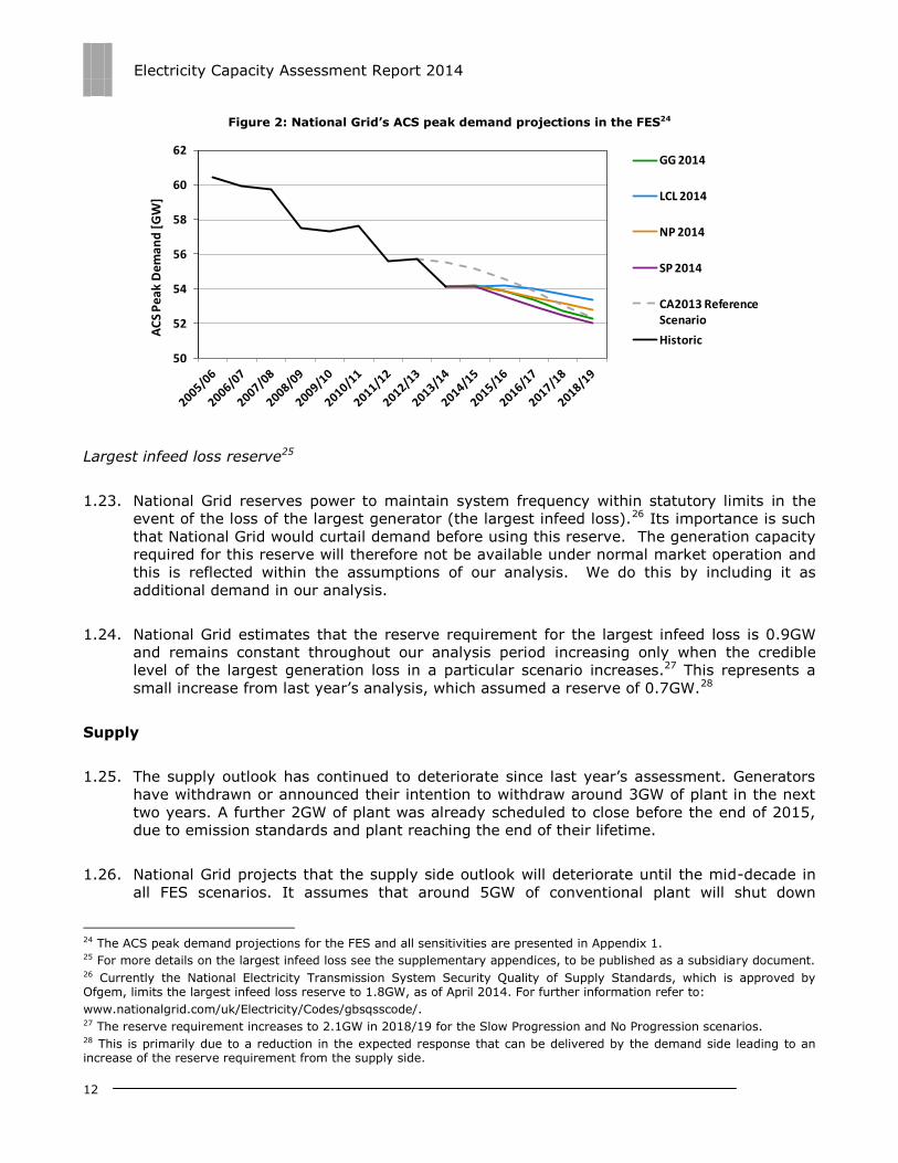
1.29. Table 1 shows the availability (ie de-rating factors) of generators per technology type for
our assessment. These are largely similar with the assumptions used in our 2013
assessment.
Table 1: Generator de-rating factors per technology type
Fuel type Availability [%]
Coal / Biomass 88%
Gas CCGT / Gas CHP 87%
OCGT 94%
Oil 82%
Nuclear 81%
Hydro 84%
Pumped Storage 97%
Interconnectors
1.30. National Grid makes assumptions about the level and direction of flows between GB and its
interconnected markets in winter. It assumes that GB will import as much as it exports. Full
exports from GB to Ireland (-750 MW) are fully compensated by imports from mainland
Europe (+750 MW). This assumption is based on analysis of historical flows since 2005/06,
feedback from industry and the outlook for our interconnected markets.
What National Grid’s scenarios mean for security of supply
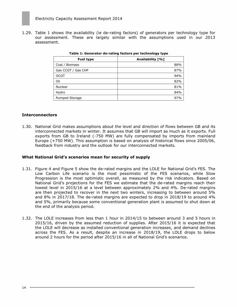
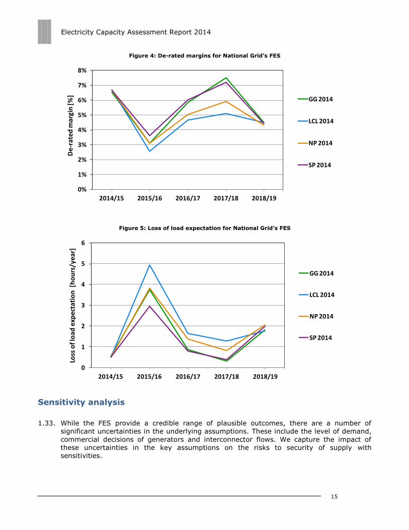
1.31. Figure 4 and Figure 5 show the de-rated margins and the LOLE for National Grid’s FES. The
Low Carbon Life scenario is the most pessimistic of the FES scenarios, while Slow
Progression is the most optimistic overall, as measured by the risk indicators. Based on
National Grid’s projections for the FES we estimate that the de-rated margins reach their
lowest level in 2015/16 at a level between approximately 2% and 4%. De-rated margins
are then projected to recover in the next two winters, increasing to between around 5%
and 8% in 2017/18. The de-rated margins are expected to drop in 2018/19 to around 4%
and 5%, primarily because some conventional generation plant is assumed to shut down at
the end of the analysis period.
1.32. The LOLE increases from less than 1 hour in 2014/15 to between around 3 and 5 hours in
2015/16, driven by the assumed reduction of supplies. After 2015/16 it is expected that
the LOLE will decrease as installed conventional generation increases, and demand declines
across the FES. As a result, despite an increase in 2018/19, the LOLE drops to below
around 2 hours for the period after 2015/16 in all of National Grid’s scenarios.
Electricity Capacity Assessment Report 2014
15
Figure 4: De-rated margins for National Grid’s FES
Figure 5: Loss of load expectation for National Grid’s FES
Sensitivity analysis
1.33. While the FES provide a credible range of plausible outcomes, there are a number of
significant uncertainties in the underlying assumptions. These include the level of demand,
commercial decisions of generators and interconnector flows. We capture the impact of
these uncertainties in the key assumptions on the risks to security of supply with
sensitivities.
0%
1%
2%
3%
4%
5%
6%
7%
8%
2014/15 2015/16 2016/17 2017/18 2018/19
De
-rat
ed
mar
gin
[%]
GG 2014
LCL 2014
NP 2014
SP 2014
0
1
2
3
4
5
6
2014/15 2015/16 2016/17 2017/18 2018/19
Loss
of l
oad
exp
ecta
tio
n [
ho
urs
/yea
r]
GG 2014
LCL 2014
NP 2014
SP 2014
Electricity Capacity Assessment Report 2014
16
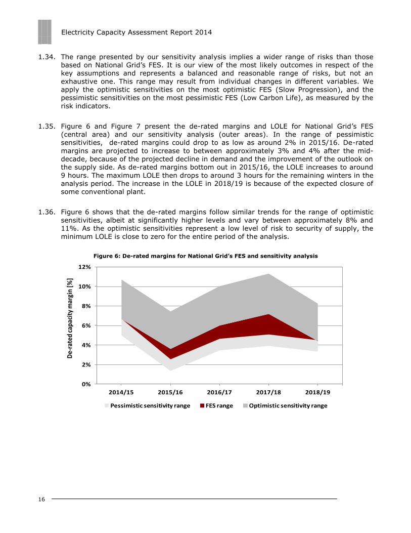
1.34. The range presented by our sensitivity analysis implies a wider range of risks than those
based on National Grid’s FES. It is our view of the most likely outcomes in respect of the
key assumptions and represents a balanced and reasonable range of risks, but not an
exhaustive one. This range may result from individual changes in different variables. We
apply the optimistic sensitivities on the most optimistic FES (Slow Progression), and the
pessimistic sensitivities on the most pessimistic FES (Low Carbon Life), as measured by the
risk indicators.
1.35. Figure 6 and Figure 7 present the de-rated margins and LOLE for National Grid’s FES
(central area) and our sensitivity analysis (outer areas). In the range of pessimistic
sensitivities, de-rated margins could drop to as low as around 2% in 2015/16. De-rated
margins are projected to increase to between approximately 3% and 4% after the mid-
decade, because of the projected decline in demand and the improvement of the outlook on
the supply side. As de-rated margins bottom out in 2015/16, the LOLE increases to around
9 hours. The maximum LOLE then drops to around 3 hours for the remaining winters in the
analysis period. The increase in the LOLE in 2018/19 is because of the expected closure of
some conventional plant.
1.36. Figure 6 shows that the de-rated margins follow similar trends for the range of optimistic
sensitivities, albeit at significantly higher levels and vary between approximately 8% and
11%. As the optimistic sensitivities represent a low level of risk to security of supply, the
minimum LOLE is close to zero for the entire period of the analysis.
Figure 6: De-rated margins for National Grid’s FES and sensitivity analysis
0%
2%
4%
6%
8%
10%
12%
2014/15 2015/16 2016/17 2017/18 2018/19
De-
rate
d ca
paci
ty m
argi
n [%
]
Pessimistic sensitivity range FES range Optimistic sensitivity range

Electricity Capacity Assessment Report 2014
17
Figure 7: LOLE for National Grid’s FES and sensitivity analysis
1.37. Below we present the rationale for the levels of variation in key variables, ie demand,
supply and interconnector flows, used for this analysis. More extreme variations could
result in a wider range but they are considered less likely than the ones explained below.
Some of the more extreme situations such a severe winter are analysed in Chapter 3.
Demand
1.38. It is inherently difficult to project how demand will evolve. This is illustrated by last winter’s
reduction in demand which was larger than expected by National Grid.32 Demand has fallen
in the period from 2005/06, primarily as a result of the economic downturn and the
implementation of energy efficiency measures. Last winter’s demand drop happened
against a backdrop of the strongest economic growth in GB since the economic crisis and
indicates that structural changes might be taking place.33 However any such changes are
not fully understood yet. There is also uncertainty about the ability of any methodology,
used to calculate the ACS peak demand, to capture the effects of very warm weather, as
experienced last winter.34
1.39. In order to take into account these uncertainties, we have developed a high demand
sensitivity that assumes peak demand is 0.75GW higher than in National Grid’s most
pessimistic scenario, in all winters. This represents approximately the proportion of last
winter’s demand drop that is not fully understood. Conversely, the low demand sensitivity
assumes a demand level 0.75GW lower, than National Grid’s most optimistic FES. It
represents a future where demand continues to decline. The change in demand equals
32 National Grid projected that demand would drop from 55.5GW in 2012/13 to 55.1GW in 2013/14 in its FES 2013. This year’s FES estimate the outturn peak demand for 2013/14 at 54.1GW. 33 Traditionally, electricity demand has been closely linked to the performance of the economy. At the same time, last year’s economic growth was mainly driven by less energy intensive sectors, for example IT services. 34 Winter 2013/14 was the fifth warmest winter since 1980; for more information see www.metoffice.gov.uk/climate/uk/summaries/2014/winter.
0
2
4
6
8
10
2014/15 2015/16 2016/17 2017/18 2018/19
Loss
of l
oad
exp
ecta
tio
n [h
ou
rs/y
ear]
Optimistic sensitivity range FES range Pessimistic sensitivity range
Electricity Capacity Assessment Report 2014
18
approximately half the demand drop for last winter demand and falls within the average
projection error by National Grid since 2009.
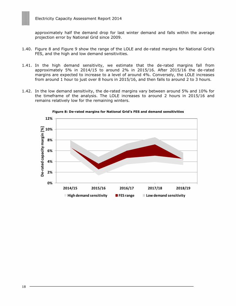
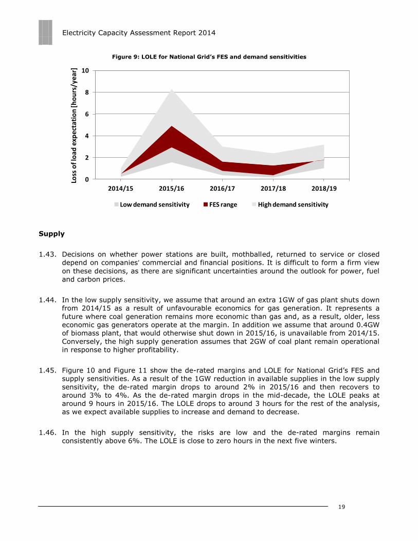
1.40. Figure 8 and Figure 9 show the range of the LOLE and de-rated margins for National Grid’s
FES, and the high and low demand sensitivities.
1.41. In the high demand sensitivity, we estimate that the de-rated margins fall from
approximately 5% in 2014/15 to around 2% in 2015/16. After 2015/16 the de-rated
margins are expected to increase to a level of around 4%. Conversely, the LOLE increases
from around 1 hour to just over 8 hours in 2015/16, and then falls to around 2 to 3 hours.
1.42. In the low demand sensitivity, the de-rated margins vary between around 5% and 10% for
the timeframe of the analysis. The LOLE increases to around 2 hours in 2015/16 and
remains relatively low for the remaining winters.
Figure 8: De-rated margins for National Grid’s FES and demand sensitivities
0%
2%
4%
6%
8%
10%
12%
2014/15 2015/16 2016/17 2017/18 2018/19
De-
rate
d c
apac
ity
mar
gin
[%
]
High demand sensitivity FES range Low demand sensitivity
Electricity Capacity Assessment Report 2014
19
Figure 9: LOLE for National Grid’s FES and demand sensitivities
Supply
1.43. Decisions on whether power stations are built, mothballed, returned to service or closed
depend on companies’ commercial and financial positions. It is difficult to form a firm view
on these decisions, as there are significant uncertainties around the outlook for power, fuel
and carbon prices.
1.44. In the low supply sensitivity, we assume that around an extra 1GW of gas plant shuts down
from 2014/15 as a result of unfavourable economics for gas generation. It represents a
future where coal generation remains more economic than gas and, as a result, older, less
economic gas generators operate at the margin. In addition we assume that around 0.4GW
of biomass plant, that would otherwise shut down in 2015/16, is unavailable from 2014/15.
Conversely, the high supply generation assumes that 2GW of coal plant remain operational
in response to higher profitability.
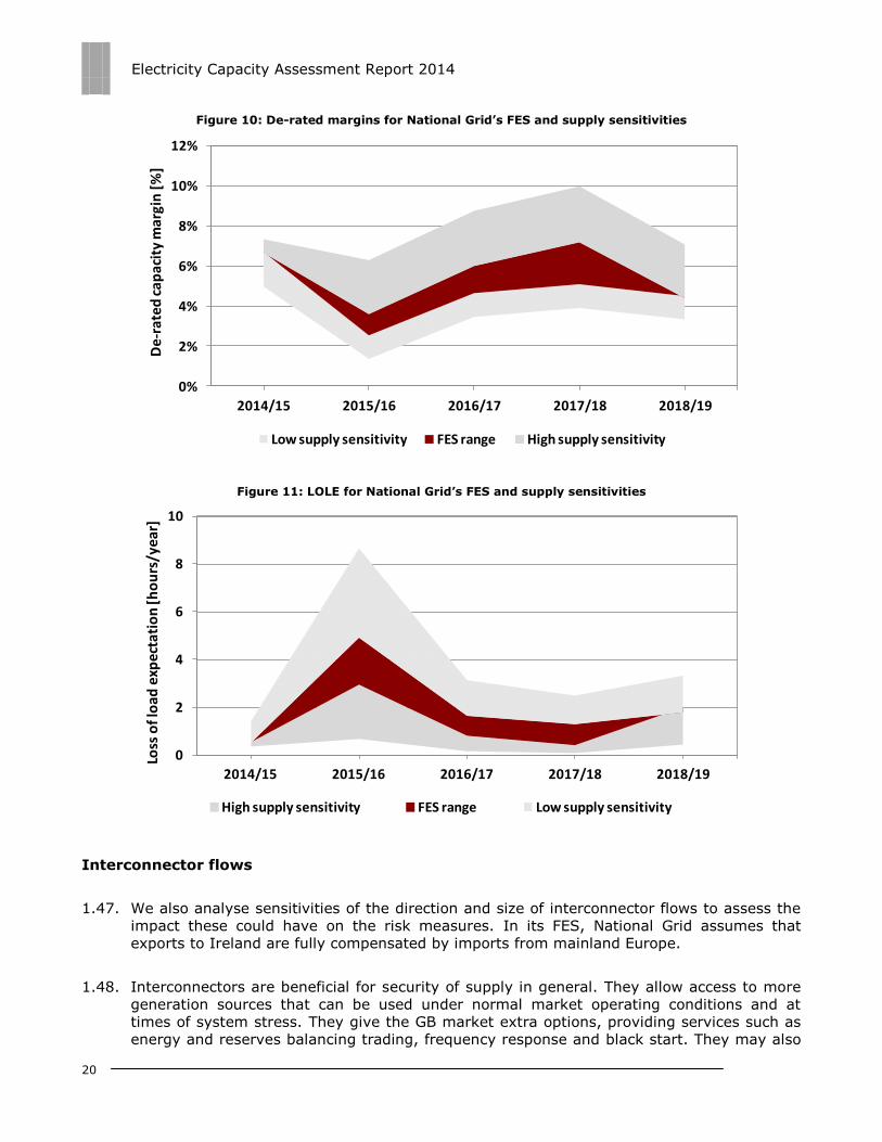
1.45. Figure 10 and Figure 11 show the de-rated margins and LOLE for National Grid’s FES and
supply sensitivities. As a result of the 1GW reduction in available supplies in the low supply
sensitivity, the de-rated margin drops to around 2% in 2015/16 and then recovers to
around 3% to 4%. As the de-rated margin drops in the mid-decade, the LOLE peaks at
around 9 hours in 2015/16. The LOLE drops to around 3 hours for the rest of the analysis,
as we expect available supplies to increase and demand to decrease.
1.46. In the high supply sensitivity, the risks are low and the de-rated margins remain
consistently above 6%. The LOLE is close to zero hours in the next five winters.
0
2
4
6
8
10
2014/15 2015/16 2016/17 2017/18 2018/19
Loss
of l
oad
exp
ect
atio
n [h
ou
rs/y
ear
]
Low demand sensitivity FES range High demand sensitivity
Electricity Capacity Assessment Report 2014
20
Figure 10: De-rated margins for National Grid’s FES and supply sensitivities
Figure 11: LOLE for National Grid’s FES and supply sensitivities
Interconnector flows
1.47. We also analyse sensitivities of the direction and size of interconnector flows to assess the
impact these could have on the risk measures. In its FES, National Grid assumes that
exports to Ireland are fully compensated by imports from mainland Europe.
1.48. Interconnectors are beneficial for security of supply in general. They allow access to more
generation sources that can be used under normal market operating conditions and at
times of system stress. They give the GB market extra options, providing services such as
energy and reserves balancing trading, frequency response and black start. They may also
0%
2%
4%
6%
8%
10%
12%
2014/15 2015/16 2016/17 2017/18 2018/19
De-
rate
d c
apac
ity
mar
gin
[%
]
Low supply sensitivity FES range High supply sensitivity
0
2
4
6
8
10
2014/15 2015/16 2016/17 2017/18 2018/19
Loss
of l
oad
exp
ecta
tio
n [h
ou
rs/y
ear]
High supply sensitivity FES range Low supply sensitivity
Electricity Capacity Assessment Report 2014
21
help reduce the cost of electricity throughout the year and transfer excess renewable
generation between countries in a future with high penetration of intermittent generation.
1.49. At times of system stress, interconnectors can reduce the probability of controlled
disconnections of customers. This is because the mitigation actions available to National
Grid to manage supply deficits include increasing the level of imports and/or reducing the
level of exports. This means disconnections would only take place after any assistance from
the interconnectors.
1.50. Full implementation of the European target model, coupled with investment in new
interconnection capacity, is expected to enable a single market in Europe. This would allow
power to flow where it’s most needed in the long term, improving security of supply overall
for Europe and the member states individually. In addition, our reforms of the electricity
balancing arrangements are expected to sharpen cash-out prices thus providing the right
signals for interconnectors to respond to higher prices when needed.35
1.51. Future interconnector flows should depend on the difference in price between GB and its
interconnected markets. This is a result of market coupling.36 As we showed in last year’s
assessment, GB and its interconnected markets have similar features.37 For example we
tend to experience peak demand at broadly the same time. The security of supply outlook
remains challenging in many markets in north-west Europe. As a result many markets are
implementing or planning to implement Capacity Markets or other measures that could give
an incentive for new investment and retain capacity that would otherwise leave the market.
The implementation of these measures will have an impact on prices making it difficult to
predict what the price differentials between GB and continental European markets will be
over the period. This increases uncertainty around interconnector flows.
1.52. GB has imported power overall from mainland Europe during the winter season in the past
two years as GB prices have generally been higher than prices in our interconnected
markets. However, given the multiple changes in the EU and GB markets, including the
implementation of market coupling, we cannot assume that flows in the coming winters will
necessarily be similar to recent flows. Based on last year’s analysis and the updated
outlook for the relevant markets to GB, we conclude that we cannot anticipate with a
sufficient degree of certainty whether continental European prices will remain below GB
prices over the analysis period. We therefore consider a range of potential level and
direction of flows as part of our sensitivity analysis.38
1.53. Interconnection capacity between GB and mainland Europe and Ireland is currently
3.8GW.39 We assume no increase in GB’s interconnection capacity over the period of this
35 We published our final policy decision for the Electricity Balancing Significant Code Review in May 2013. For more information, see: www.ofgem.gov.uk/electricity/wholesale-market/market-efficiency-review-and-reform/electricity-balancing-significant-code-review. 36 Market coupling was implemented across North-West Europe, including GB, in February 2014. 37 For more information see Pöyry’s analysis for the Electricity Capacity Assessment 2013 report, available here: www.ofgem.gov.uk/publications-and-updates/p%C3%B6yry-analysis-correlation-tight-periods-electricity-markets-gb-and-its-interconnected-systems. 38 For more information on our approach on interconnectors and the outlook for the relevant markets to GB see the supplementary appendices, to be published as a subsidiary document. 39 Currently, a number of projects are at various stages of development and could complete in the timeframe of our analysis. However, there is high uncertainty on whether and when these projects might become operational (eg this will

Electricity Capacity Assessment Report 2014
22
analysis. We assume that the interconnectors will export to Ireland at full capacity
(0.75GW) in all sensitivities. Our pessimistic sensitivity assumes that we do not import or
export to mainland Europe (no imports sensitivity). This situation could occur if, for
example a cold winter occurs in France causing their prices to rise above those in GB. Our
optimistic sensitivity assumes full imports of 3GW from mainland Europe (full imports
sensitivity). This could occur if there was a surplus of cheaper power in our interconnected
markets.
1.54. Figure 12 and Figure 13 show the de-rated margins and LOLE for the FES scenario range
and the interconnector flow sensitivities. In the ‘no imports sensitivity’, the de-rated
margins bottom out at around 2% in 2015/16 before they recover at levels between around
3% and 4%. The LOLE peaks at around 8 hours in 2015/16. The risks are estimated to
decrease after the mid-decade, with the LOLE declining to around 3 hours.
1.55. In the ‘full imports sensitivity’ the risks to security of supply would be significantly lower
with de-rated margins higher than 7% in all winters. The LOLE follows a similar trend
across the analysis period but remains close to zero in all winters.
Figure 12: De-rated margins for National Grid’s FES and interconnector flow sensitivities
depend on them receiving the necessary application agreements) and hence, we assume no increase in our interconnected capacity.
0%
2%
4%
6%
8%
10%
12%
2014/15 2015/16 2016/17 2017/18 2018/19
De-
rate
d c
apac
ity
mar
gin
[%
]
No imports sensitivity FES range Full imports sensitivity

Electricity Capacity Assessment Report 2014
23
Figure 13: LOLE for National Grid’s FES and interconnector flow sensitivities
Potential impact on customers
1.56. If demand is higher than supply under normal operation of the system, National Grid as the
System Operator can use mitigation actions to manage supply shortfalls, with little or no
impact on customers in most cases. These actions include voltage control, requesting
maximum generation from plant or requesting emergency services from the
interconnectors. The new balancing services give National Grid an additional tool to balance
the system before using these mitigation actions. National Grid will hold these services
outside the market and would only use them after all normal market options have been
exhausted (and before any other mitigation action).40
1.57. As these mitigation actions, including the new balancing services, are held outside the
market, they do not impact either the LOLE or the de-rated margins calculations. This is
because these indicators are measured at the end of normal market operations (ie at the
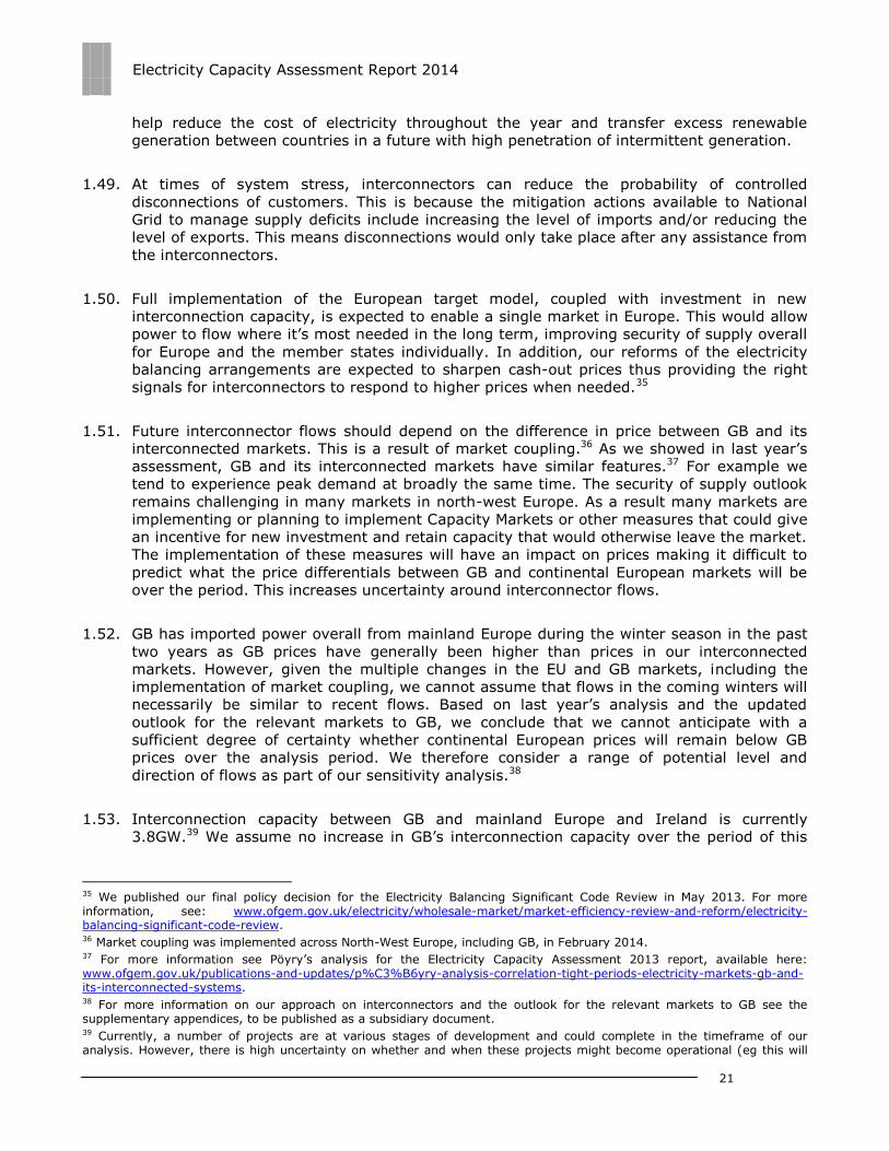
end of the Balancing Market), as is depicted in Figure 14 below. Once the new balancing
services have been implemented they will lower the likelihood of controlled disconnections.
40 This is in circumstances where it was already clear to National Grid that they would be unable to balance supply and demand based on bids and offers from the balancing market. For more information on the new balancing services see www.nationalgrid.com/uk/electricity/additionalmeasures.
0
2
4
6
8
10
2014/15 2015/16 2016/17 2017/18 2018/19
Loss
of l
oad
exp
ect
ati
on
[ho
urs
/ye
ar]
Full imports sensitivity FES range No imports sensitivity
Electricity Capacity Assessment Report 2014
24
Figure 14: Electricity market, mitigation actions and the LOLE and 1 in n metrics
1.58. Controlled disconnections would therefore only take place if a large supply deficit were to
occur. To illustrate the potential impact on customers, we estimate the probability of such
an event happening, before and after the implementation of the new balancing services.
We do this using the 1 in n year indicator – this is only an approximation as there are
significant uncertainities on the availability and size of the mitigation actions.
1.59. Without the New Balancing Services, the expected risks of customer disconnections would
vary between approximately once every 8 years (1 in 8 years) and once every four years
(1 in 4 years) in 2015/16 for National Grid’s FES. However, if National Grid procured the
maximum volume of new balancing services it has indicated for 2015/16,41 the additional
measures would reduce the risk of disconnections to up to around 1 in 73 and 1 in 31 years
for the FES. This is better than the probability of controlled disconnections that corresponds
to the reliability standard for that year (which is 1-in-8 years in winter 2015/16), and
within the range of forward looking risks we identified for recent winters in our previous
assessments.
Historical context to the risks to security of supply
1.60. The GB electricity market experienced low levels of security of supply risks in the last
decade or so with de-rated margins increasing from 2005/06 to 2010/11. Since 2010/11,
de-rated margins have been gradually declining. The range expected for winter 2015/16
(around 2% to 8%) is around the level experienced in 2005/06.
1.61. However, the level of risk associated with a given de-rated margin would be higher today
than it was in that period. This is because of the increased amount of intermittent
generation, such as wind in the GB system. Table 2 presents the evolution of de-rated
margins and the corresponding LOLE for a number of years in the last decade.42 The risks
presented in this table should not be interpreted as the realised loss of load in these
41 National Grid has confirmed its intention to procure a maximum of around 0.3GW and 1.8GW of these services in 2014/15 and 2015/16 respectively. 42 The assumptions behind the historical indices calculations are presented in the supplementary appendices, to be
published as a subsidiary document.
Supply available in the normal market operation up to Balancing Mechanism
New Balancing Services
Voltage Reduction –
up to 500 MW
Maximum Generation –up to 250 MW
Emergency Services from
interconnectors –up to 2000 MW
(depending on direction and size of
flows)
Controlled Disconnections
Market supply Exceeds demand
Demand exceedsMarket supply
Actions that would take place during loss of load events
Measured by 1 in n
Electricity Capacity Assessment Report 2014
25
winters, but rather as the expected risks associated with the actual characteristics of the
GB market in these winters.43
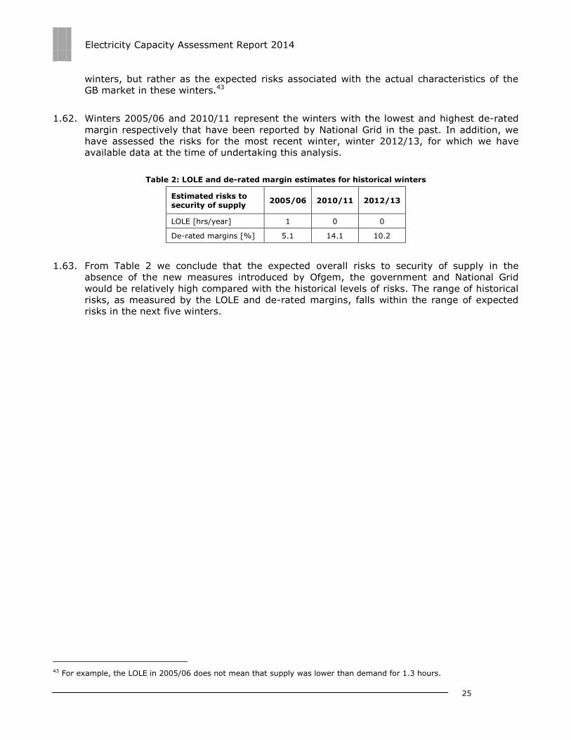
1.62. Winters 2005/06 and 2010/11 represent the winters with the lowest and highest de-rated
margin respectively that have been reported by National Grid in the past. In addition, we
have assessed the risks for the most recent winter, winter 2012/13, for which we have
available data at the time of undertaking this analysis.
Table 2: LOLE and de-rated margin estimates for historical winters
Estimated risks to security of supply
2005/06 2010/11 2012/13
LOLE [hrs/year] 1 0 0
De-rated margins [%] 5.1 14.1 10.2
1.63. From Table 2 we conclude that the expected overall risks to security of supply in the
absence of the new measures introduced by Ofgem, the government and National Grid
would be relatively high compared with the historical levels of risks. The range of historical
risks, as measured by the LOLE and de-rated margins, falls within the range of expected
risks in the next five winters.
43 For example, the LOLE in 2005/06 does not mean that supply was lower than demand for 1.3 hours.

Electricity Capacity Assessment Report 2014
26
2. Methodology
2.1. This chapter provides a brief, high-level description of the methodology used for this
report. We explain the indicators and modelling approach used to assess the risk to
electricity security of supply in GB and the key differences between scenarios and
sensitivities. A detailed description of the modelling approach can be found in our 2013
report.44
2.2. As in our past two assessments, the 2014 report uses a combination of a probabilistic
approach and sensitivity analysis to capture uncertainty. We use a probabilistic model to
calculate the risk indicators. This takes into account the uncertainty related to short-term
variations in demand and available conventional generation resulting from outages and
wind generation. These are uncertainties that can be quantified with a good degree of
credibility based on historical information. The probabilistic approach is combined with
sensitivity analysis to capture uncertainties that cannot be given any credible probabilities.
Indicators
2.3. We use five indicators to assess the outlook for electricity security of supply. These are
described below. Tables with the results for all five indicators can be found in Appendix 145.
Loss of load expectation (LOLE): the average mean number of hours per year in which
supply does not meet demand in the absence of intervention46 from the System
Operator.
De-rated capacity margin: the average excess of available generation capacity over
peak demand, expressed in percentage terms and capacity in MW.
Expected Energy Unserved (EEU): the expected amount of electricity demand that
would not be met in a year due to loss of load incidents. EEU combines both the
likelihood and the potential size of any supply shortfall and is measured at the same
point of market operations (ie at the end of normal market operations) with LOLE.
1 in n probability of controlled disconnections: an illustration of the results of the LOLE
in terms of tangible impacts for electricity customers. It is not as accurate as the LOLE
and EEU but it allows us to provide a view of the likelihood of experiencing controlled
disconnections of customers.
Equivalent Firm Capacity of wind (EFC): the average contribution of wind power to
the de-rated margin. It is the quantity of firm capacity (ie always available) required
to replace the wind generation in the system to give the same level of security of
44 The 2013 document can be found here: www.ofgem.gov.uk/ofgem-publications/75232/electricity-capacity-assessment-report-2013.pdf. 45 For the 1 in n metric results see the supplementary appendices, to be published as a subsidiary document. 46 The supplementary appendices explain the mitigation actions available to National Grid to intervene before implementing controlled disconnections of customers. The new balancing services are an addition to this set of tools and are also explained in these appendices.
Electricity Capacity Assessment Report 2014
27
supply, as measured by LOLE. It varies with the proportion of wind power in the
system and with regards to the generation and demand assumptions for a scenario
and sensitivity.
Modelling approach
2.4. We use the Capacity Assessment probabilistic model to analyse capacity adequacy in GB.
This is the same model used for previous Capacity Assessment reports. We concentrate the
analysis in the winter period as given the current structure of the GB market it is unlikely to
experience loss of load events during summer. We also assume there is sufficient gas in the
system to operate all gas fired power stations and that transmission constraints do not
represent a risk for security of supply.
2.5. These assumptions have been validated by the summer analysis, the transmission
boundary constraint analysis and the gas stress test which are briefly described below.47
Summer analysis: presents de-rated capacity margins under summer conditions, ie
using summer peak demand and summer plant availability.
Transmission boundary constraint analysis: analyses the potential impact of the most
constrained transmission network boundary48 on the security of supply indicators.
Gas stress test: analyses the impact of a drop in gas supplies to GB on the security of
supply indicators.
2.6. Our model is a time-collapsed model; this means that it calculates the probability of
demand exceeding available supply (supply deficit) at a randomly chosen half-hour from
the winter period. It uses a distribution of demand during winter season. Times of
extremely high demand that might require National Grid to use mitigation actions are
represented in the tails of the demand distribution. Below we briefly describe how our
probabilistic model estimates the five indicators. A more detailed description of the
methodology can be found in our 2013 report.
LOLE and EEU
2.7. To calculate the LOLE and EEU, in the five winter modelling period, the model constructs
probability distributions of winter demand49, wind power and available conventional
generation. The LOLE and EEU are calculated by combining (ie through convolution50) the
three distributions; this represents the main risk calculation. The outcome of the
convolution is a distribution of margins (ie the difference between supply and demand) for
47 These analyses are included in the supplementary appendices, to be published as a subsidiary document. 48 The Cheviot boundary between Scotland and England. 49 Winter demand is based on Average Cold Spell (ACS) demand. This reflects the combination of weather elements (ie temperature, illumination and wind) that give rise to a level of peak demand within a financial year that has a 50% chance of being exceeded as a result of weather variations alone. 50 Convolution is the mathematical operation of obtaining the distribution of the sum of two independent random variables from their individual distributions.

Electricity Capacity Assessment Report 2014
28
each winter in the modelling period. The LOLE and EEU are then estimated from the part of
the distribution for which supply is lower than demand under normal market operations.
2.8. LOLE does not represent the expected number of hours that customers will be
disconnected.51 It is defined as the expected number of hours that supply will not meet
demand under normal operations of the market. This is equivalent to the number of hours
in a year in which National Grid would have to use mitigation actions, (ie actions beyond
normal market operations), to balance supply and demand.52 The definition of LOLE in our
assessment is consistent with the Electricity Capacity Regulations for the Capacity Market.53
De-rated margins and Equivalent Firm Capacity of wind
2.9. The de-rated margin is calculated by subtracting the adjusted peak demand from the
typical available capacity in the system. This produces the margin in MW which is then
divided by the adjusted peak demand to express the margin as a percentage of peak
demand.
2.10. The adjusted peak demand is the ACS peak demand, where the reserve for the largest
infeed loss54 and the net flows on interconnectors (positive for net export, negative for net
imports) are added to it.55 The typical available capacity is the sum of the average available
conventional capacity (installed conventional capacity times de-rating factors) and the EFC
of wind generation, including embedded wind.
2.11. The EFC is the quantity of firm capacity (ie always available) that can be replaced by a
certain volume of wind generation to give the same level of security of supply, as measured
by LOLE. It is measured in both percentage terms (as a proportion of installed wind
capacity) and capacity (representing the amount of firm capacity in MW).
1 in n probability of disconnections
2.12. LOLE is not a measure of the expected number of hours per year in which customers may
be disconnected as most of the time National Grid can implement mitigation actions to
solve capacity adequacy problems without disconnecting any customers. To illustrate the
potential impact on customers, we estimate the frequency of outages of a given severity
when mitigation actions available to the System Operator have been exhausted.
2.13. The 1 in n years estimate is an approximation only, rather than a model output. We have
insufficient data available to allow us to perform a precise calculation as there have not
been any disconnections caused by lack of adequate capacity in recent years. The estimate
is therefore based on judgments as to how the electricity system would operate where
available supply does not meet demand. We also estimate the order and size of mitigation
51 Similarly, EEU does not represent the amount of energy that will not be delivered to customers. 52 Likewise, the de-rated margins and EEU are estimated at the end of normal market operations. 53 Available in (page 9): www.gov.uk/government/uploads/system/uploads/attachment_data/file/249564/electricity_capacity_regulations_2014_si.pdf 54 This is the generation that National Grid reserves to maintain system frequency within statutory limits in the event of the loss of the largest generator. 55 For details on how these variables are treated see our 2013 report, appendix 3.

Electricity Capacity Assessment Report 2014
29
actions taken by the System Operator (eg how much extra generation can be available if
maximum generation is implemented). It is not as accurate as the LOLE and EEU but it
allows us to provide a view of the likelihood of experiencing controlled disconnections of
customers. The ‘n’ represents the average number of years between these events.56
2.14. To estimate the 1 in n we use the tail of the de-rated margin distribution produced by the
probabilistic model, which corresponds to the LOLE, and assume that the relative
frequencies of loss of load events of different sizes and durations match the shape of that
tail. We then find the likely frequency of large events that matches the extreme of the LOLE
shape which represents the probability of customer disconnections.57
Inputs
2.15. Our probabilistic model uses the following input data that are based on analysis by National
Grid:
demand, including ACS peak demand, historical demand data and the reserve for the
largest infeed loss;
installed conventional generation and the de-rating factors per technology type;
wind generation, including installed capacity and location of transmission connected
and embedded wind farms and historical wind speeds; and
interconnector flows.
2.16. We have broadly retained the same methodology for estimating the input assumptions;
details can be found in our 2013 report (appendix 3). We have varied the methodology for
estimating the de-rating factor for gas plant.58
Scenarios and Sensitivities
2.17. Our analysis is based on National Grid’s four FES. This is a change from our 2013
assessment that was based on the Gone Green scenario, adjusted to reflect our own views
on interconnector flows and the supply-side evolution under policy uncertainty. As in our
previous assessments, we have developed sensitivity analysis about the key uncertainties
in the input assumptions. Below we describe the differences between scenarios and
sensitivities.
2.18. A scenario represents an alternative possible future59, taking into account how the system
might evolve as a whole. Scenarios are designed to be internally consistent, which means
56 For example, a frequency of controlled disconnections of 1 in 2 years means that controlled disconnection events may occur once every 2 years if the system remains unchanged. The larger the n the smaller the probability of controlled disconnections which is better for customers. 57 This is a change from the previous two years, where we used a power law to calculate the relative frequencies of shortfall events. For more information, see supplementary appendices, to be published as a subsidiary document. 58 Details can be found in the supplementary appendices.

Electricity Capacity Assessment Report 2014
30
that the relationships and dependencies between the variables that represent the system
are taken into account (eg generation responding to long-term demand trends). The
purpose of scenario analysis is to provide a range of possible future outcomes with regards
to a set of key drivers (eg fuel prices, sustainability) and not to predict the future.
2.19. Our sensitivity analysis aims to assess the impact of uncertainty of just one assumption on
the risks to security of supply. Each sensitivity represents a change in a single variable
from a scenario, with all other assumptions being held constant. This means, unlike a
scenario where every variable would respond, everything else remains the same and the
system is not necessarily internally consistent (eg we do not consider how generation could
react if demand was higher or lower than in any particular scenario). We do this to assess
the impact on the risk measures of the uncertainty related to each variable in isolation.
2.20. Through our pessimistic and optimistic sensitivity analysis we identify the downside (ie
what could be worse) and upside risks (ie what could be better) respectively that could
have an impact on the outlook for security of supply. We apply the downside risks on
National Grid’s most pessimistic scenario (Low Carbon Life 2014) and the upside risks on
National Grid’s most optimistic scenario (Slow Progression 2014), as measured by the risk
indicators. In the next chapter we discuss the complete sensitivity analysis we have
undertaken for this assessment.
59 For example the Gone Green scenario represents a future where sustainability is at the centre, while the No Progression scenario represents a future that resembles the present.
Electricity Capacity Assessment Report 2014
31
3. Wider range of sensitivities
3.1. In Chapter 1, we presented the risks to security of supply implied by National Grid’s FES
and a central range of risks resulting from our sensitivity analysis around it. The range
presented in Chapter 1 provides a balanced and reasonable assessment of the risks around
National Grid’s scenarios based on our view of the most likely outcomes.
3.2. In this chapter, we present a fuller range of sensitivities that are less likely but still possible
and relevant to analyse for the security of supply outlook. Some of these sensitivities are
statistically less likely, like a colder than average winter. Others consider less likely
situations; for example a large number of plant mothballing simultaneously would probably
trigger a response from the market that is not represented in our sensitivities. We do not
cover the full range of potential variations in the key assumptions to include sensitivities
that would result in negative de-rated margins as we consider this possibility unrealistic. If
such an event did occur for a sustained period, higher prices and a market response would
be expected. This response could manifest in a number of ways, such as increased
availability of plant or higher imports from our interconnected markets, among others.
3.3. The fuller range of sensitivities covers wider possible outcomes for demand, plant closure
and mothballing decisions by generators, and the level and direction of interconnector
flows. We also present sensitivities on the availability of conventional and variable
generation and winter weather conditions. We explain the assumptions underpinning these
sensitivities and the risks to security of supply associated with them below. Given the high
degree of uncertainty about the market evolution, it is important that decisions taken are
robust not only with regards to a central scenario but also to potential ranges of variation
around it.
Wider range of sensitivities
3.4. The range of risks presented in Chapter 1 covers our views of the most likely outcomes
around the key uncertainties, ie peak demand level, commercial decisions of generators
and flows with our interconnected markets. This results in a range of de-rated margins
between around 2% and 8% in 2015/16, corresponding to an LOLE between 0 and 9 hours
in the same year. We estimate that the risks to security of supply decrease after the mid-
decade, as the outlook for electricity supplies is assumed to improve and demand continues
to decrease. There is an increase in risk again for 2018/19, although not to the 2015/16
levels, as some conventional generation plant closes. The projected range of de-rated
margins varies between around 3% and 8% in that year, corresponding to an LOLE range
between 0 and 3 hours.
3.5. Figure 15 and Figure 16 present the de-rated margins and LOLE for the complete sensitivity
range, including the range presented in Chapter 1, and National Grid’s FES. The ranges in
these figures are produced by changes to individual variables and not by a combination of
changes to more than one variable.
3.6. Figure 15 shows that the de-rated margins could drop to close to zero in 2015/16 for the
more pessimistic sensitivity range, if for example more plant shut down or demand was
significantly higher than projected by National Grid. The de-rated margins improve after
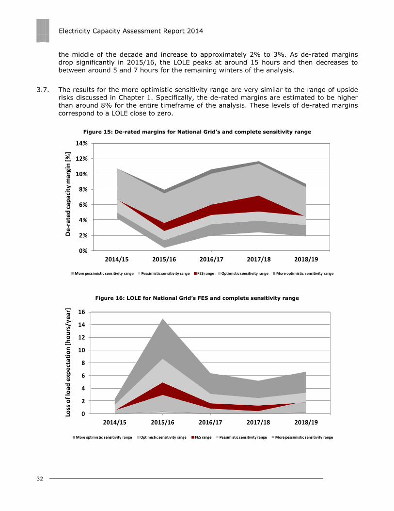
Electricity Capacity Assessment Report 2014
32
the middle of the decade and increase to approximately 2% to 3%. As de-rated margins
drop significantly in 2015/16, the LOLE peaks at around 15 hours and then decreases to
between around 5 and 7 hours for the remaining winters of the analysis.
3.7. The results for the more optimistic sensitivity range are very similar to the range of upside
risks discussed in Chapter 1. Specifically, the de-rated margins are estimated to be higher
than around 8% for the entire timeframe of the analysis. These levels of de-rated margins
correspond to a LOLE close to zero.
Figure 15: De-rated margins for National Grid’s and complete sensitivity range
Figure 16: LOLE for National Grid’s FES and complete sensitivity range
0%
2%
4%
6%
8%
10%
12%
14%
2014/15 2015/16 2016/17 2017/18 2018/19
De
-rat
ed
cap
acit
y m
argi
n [
%]
More pessimistic sensitivity range Pessimistic sensitivity range FES range Optimistic sensitivity range More optimistic sensitivity range
0
2
4
6
8
10
12
14
16
2014/15 2015/16 2016/17 2017/18 2018/19
Loss
of
loa
d e
xpe
cta
tio
n [
ho
urs
/ye
ar]
More optimistic sensitivity range Optimistic sensitivity range FES range Pessimistic sensitivity range More pessimistic sensitivity range
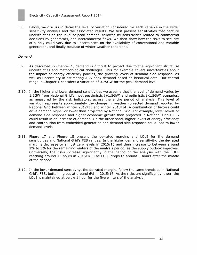
Electricity Capacity Assessment Report 2014
33
3.8. Below, we discuss in detail the level of variation considered for each variable in the wider
sensitivity analysis and the associated results. We first present sensitivities that capture
uncertainties on the level of peak demand, followed by sensitivities related to commercial
decisions by generators, and interconnector flows. We then show how the risks to security
of supply could vary due to uncertainties on the availability of conventional and variable
generation, and finally because of winter weather conditions.
Demand
3.9. As described in Chapter 1, demand is difficult to project due to the significant structural
uncertainties and methodological challenges. This for example covers uncertainties about
the impact of energy efficiency policies, the growing levels of demand side response, as
well as uncertainty in estimating ACS peak demand based on historical data. Our central
range in Chapter 1 considers a variation of 0.75GW for the peak demand level.
3.10. In the higher and lower demand sensitivities we assume that the level of demand varies by
1.5GW from National Grid’s most pessimistic (+1.5GW) and optimistic (-1.5GW) scenarios,
as measured by the risk indicators, across the entire period of analysis. This level of
variation represents approximately the change in weather corrected demand reported by
National Grid between winter 2012/13 and winter 2013/14. A combination of factors could
drive demand higher or lower than projected by National Grid. For example, lower levels of
demand side response and higher economic growth than projected in National Grid’s FES
could result in an increase of demand. On the other hand, higher levels of energy efficiency
and contribution from embedded generation and demand side response could lead to lower
demand levels.
3.11. Figure 17 and Figure 18 present the de-rated margins and LOLE for the demand
sensitivities and National Grid’s FES ranges. In the higher demand sensitivity, the de-rated
margins decrease to almost zero levels in 2015/16 and then increase to between around
2% to 3% for the remaining winters of the analysis period, as the supply outlook improves.
Conversely, the risks increase significantly in the period of the analysis with the LOLE
reaching around 13 hours in 2015/16. The LOLE drops to around 5 hours after the middle
of the decade.
3.12. In the lower demand sensitivity, the de-rated margins follow the same trends as in National
Grid’s FES, bottoming out at around 6% in 2015/16. As the risks are significantly lower, the
LOLE is maintained at below 1 hour for the five winters of the analysis.
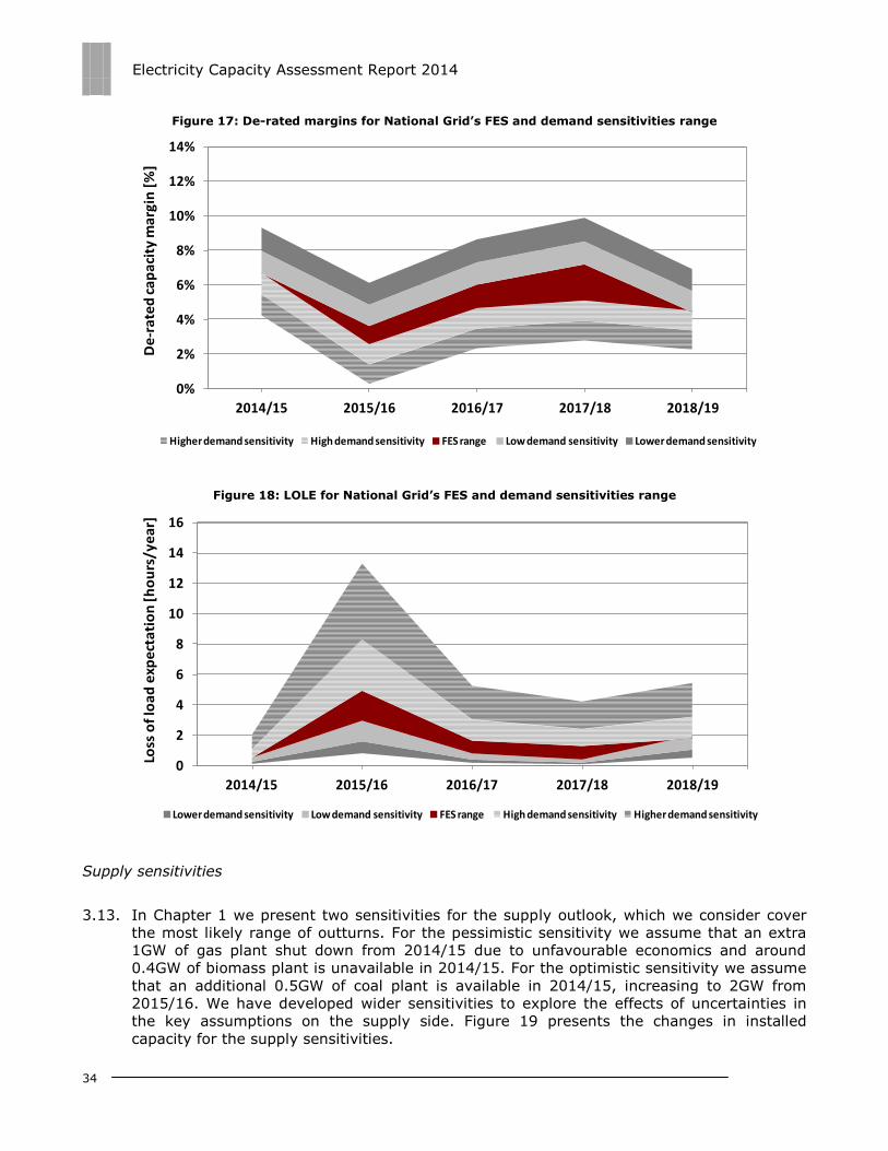
Electricity Capacity Assessment Report 2014
34
Figure 17: De-rated margins for National Grid’s FES and demand sensitivities range
Figure 18: LOLE for National Grid’s FES and demand sensitivities range
Supply sensitivities
3.13. In Chapter 1 we present two sensitivities for the supply outlook, which we consider cover
the most likely range of outturns. For the pessimistic sensitivity we assume that an extra
1GW of gas plant shut down from 2014/15 due to unfavourable economics and around
0.4GW of biomass plant is unavailable in 2014/15. For the optimistic sensitivity we assume
that an additional 0.5GW of coal plant is available in 2014/15, increasing to 2GW from
2015/16. We have developed wider sensitivities to explore the effects of uncertainties in
the key assumptions on the supply side. Figure 19 presents the changes in installed
capacity for the supply sensitivities.
0%
2%
4%
6%
8%
10%
12%
14%
2014/15 2015/16 2016/17 2017/18 2018/19
De
-ra
ted
ca
pa
city
ma
rgin
[%
]
Higher demand sensitivity High demand sensitivity FES range Low demand sensitivity Lower demand sensitivity
0
2
4
6
8
10
12
14
16
2014/15 2015/16 2016/17 2017/18 2018/19
Loss
of
loa
d e
xpe
cta
tio
n [
ho
urs
/ye
ar]
Lower demand sensitivity Low demand sensitivity FES range High demand sensitivity Higher demand sensitivity
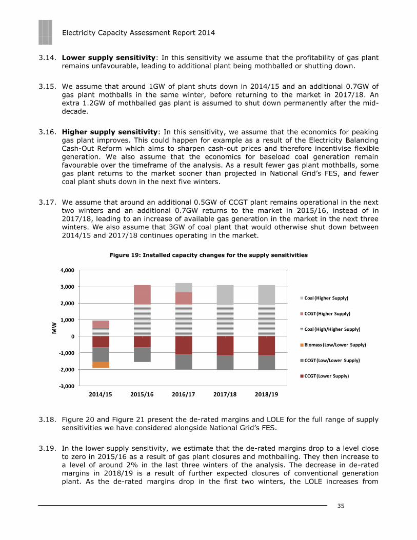
Electricity Capacity Assessment Report 2014
35
3.14. Lower supply sensitivity: In this sensitivity we assume that the profitability of gas plant
remains unfavourable, leading to additional plant being mothballed or shutting down.
3.15. We assume that around 1GW of plant shuts down in 2014/15 and an additional 0.7GW of
gas plant mothballs in the same winter, before returning to the market in 2017/18. An
extra 1.2GW of mothballed gas plant is assumed to shut down permanently after the mid-
decade.
3.16. Higher supply sensitivity: In this sensitivity, we assume that the economics for peaking
gas plant improves. This could happen for example as a result of the Electricity Balancing
Cash-Out Reform which aims to sharpen cash-out prices and therefore incentivise flexible
generation. We also assume that the economics for baseload coal generation remain
favourable over the timeframe of the analysis. As a result fewer gas plant mothballs, some
gas plant returns to the market sooner than projected in National Grid’s FES, and fewer
coal plant shuts down in the next five winters.
3.17. We assume that around an additional 0.5GW of CCGT plant remains operational in the next
two winters and an additional 0.7GW returns to the market in 2015/16, instead of in
2017/18, leading to an increase of available gas generation in the market in the next three
winters. We also assume that 3GW of coal plant that would otherwise shut down between
2014/15 and 2017/18 continues operating in the market.
Figure 19: Installed capacity changes for the supply sensitivities
3.18. Figure 20 and Figure 21 present the de-rated margins and LOLE for the full range of supply
sensitivities we have considered alongside National Grid’s FES.
3.19. In the lower supply sensitivity, we estimate that the de-rated margins drop to a level close
to zero in 2015/16 as a result of gas plant closures and mothballing. They then increase to
a level of around 2% in the last three winters of the analysis. The decrease in de-rated
margins in 2018/19 is a result of further expected closures of conventional generation
plant. As the de-rated margins drop in the first two winters, the LOLE increases from
-3,000
-2,000
-1,000
0
1,000
2,000
3,000
4,000
2014/15 2015/16 2016/17 2017/18 2018/19
MW
Coal (Higher Supply)
CCGT (Higher Supply)
Coal (High/Higher Supply)
Biomass (Low/Lower Supply)
CCGT (Low/Lower Supply)
CCGT (Lower Supply)

Electricity Capacity Assessment Report 2014
36
around 3 hours in 2014/15 to around 13 hours in 2015/16. The LOLE then recovers and
varies between 5 and 7 hours in the remaining winters of the analysis.
3.20. In the higher supply sensitivity, the risks to security of supply are very low and the de-
rated margins are maintained at levels of around 10% and above. The LOLE is close to zero
for the entire period.
Figure 20: De-rated margins for National Grid’s FES and supply sensitivities range
Figure 21: LOLE for National Grid’s FES and supply sensitivities range
0%
2%
4%
6%
8%
10%
12%
14%
2014/15 2015/16 2016/17 2017/18 2018/19
De-
rate
d c
apac
ity
mar
gin
[%
]
Lower supply sensitivity Low supply sensitivity FES range High supply sensitivity Higher supply sensitivity
0
2
4
6
8
10
12
14
16
2014/15 2015/16 2016/17 2017/18 2018/19
Loss
of
load
exp
ect
atio
n [h
ou
rs/y
ear
]
Higher supply sensitivity High supply sensitivity FES range Low supply sensitivity Lower supply sensitivity

Electricity Capacity Assessment Report 2014
37
Interconnector flows
3.21. As discussed in Chapter 1, National Grid assumes overall float for interconnectors to GB in
each of the FES. In all interconnector flow sensitivities, we assume full exports to Ireland
(0.75GW) and vary the assumption of flows with mainland Europe. In Chapter 1, we
consider a ‘no imports’ sensitivity on the pessimistic side and a ‘full imports’ sensitivity on
the optimistic side.
3.22. In addition to these, we have developed an exports sensitivity, which assumes 0.75GW of
exports to mainland Europe (corresponding to net exports of 1.5GW). Exports could happen
for example if a supply deficit occurred in France, driving their power prices above ours. We
do not find net exports for the whole winter larger than the export sensitivity to be a
credible outcome. If such an event did occur for a sustained period, higher prices and a
market response would be expected. This response could manifest in a number of ways,
such as increased availability of plant. There is no wider range of sensitivities on
interconnectors for the optimistic range as full imports are already considered as part of the
central range.
3.23. Figure 22 and Figure 23 present the de-rated margins and LOLE ranges for the
interconnector sensitivities and National Grid’s FES. In the low exports sensitivity, the de-
rated margins bottom out at a level close to zero in 2015/16, before they recover to
between close to 2% and 3% as the risks to security of supply decrease. The LOLE peaks at
around 14 hours in 2015/16, and then drops to between around 4 to 6 hours.
3.24. For the full import sensitivity, the de-rated margins vary between around 8% and 12% and
LOLE is close to zero for the timeframe of the analysis. This illustrates the significant
impact that interconnector flows can have on security of supply.
Figure 22: De-rated margins for National Grid’s FES and interconnector flow sensitivities range
0%
2%
4%
6%
8%
10%
12%
14%
2014/15 2015/16 2016/17 2017/18 2018/19
De
-rat
ed
cap
acit
y m
argi
n [
%]
Low exports sensitivity No imports sensitivity FES range Full imports sensitivity
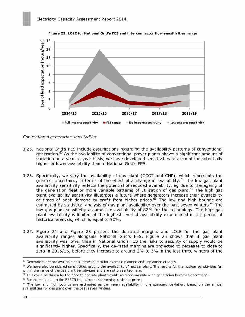
Electricity Capacity Assessment Report 2014
38
Figure 23: LOLE for National Grid’s FES and interconnector flow sensitivities range
Conventional generation sensitivities
3.25. National Grid’s FES include assumptions regarding the availability patterns of conventional
generation.60 As the availability of conventional power plants shows a significant amount of
variation on a year-to-year basis, we have developed sensitivities to account for potentially
higher or lower availability than in National Grid’s FES.
3.26. Specifically, we vary the availability of gas plant (CCGT and CHP), which represents the
greatest uncertainty in terms of the effect of a change in availability.61 The low gas plant
availability sensitivity reflects the potential of reduced availability, eg due to the ageing of
the generation fleet or more variable patterns of utilisation of gas plant.62 The high gas
plant availability sensitivity illustrates a future where generators increase their availability
at times of peak demand to profit from higher prices.63 The low and high bounds are
estimated by statistical analysis of gas plant availability over the past seven winters.64 The
low gas plant sensitivity assumes an availability of 82% for the technology. The high gas
plant availability is limited at the highest level of availability experienced in the period of
historical analysis, which is equal to 90%.
3.27. Figure 24 and Figure 25 present the de-rated margins and LOLE for the gas plant
availability ranges alongside National Grid’s FES. Figure 25 shows that if gas plant
availability was lower than in National Grid’s FES the risks to security of supply would be
significantly higher. Specifically, the de-rated margins are projected to decrease to close to
zero in 2015/16, before they increase to around 2% to 3% in the last three winters of the
60 Generators are not available at all times due to for example planned and unplanned outages. 61 We have also considered sensitivities around the availability of nuclear plant. The results for the nuclear sensitivities fall within the range of the gas plant sensitivities and are not presented here. 62 This could be driven by the need to operate plant flexibly as more variable wind generation becomes operational. 63 For example due to the EBSCR that aims at sharpening cash-out prices. 64 The low and high bounds are estimated as the mean availability ± one standard deviation, based on the annual availabilities for gas plant over the past seven winters.
0
2
4
6
8
10
12
14
16
2014/15 2015/16 2016/17 2017/18 2018/19
Loss
of l
oad
exp
ect
atio
n [h
ou
rs/y
ear
]
Full imports sensitivity FES range No imports sensitivity Low exports sensitivity

Electricity Capacity Assessment Report 2014
39
analysis. As the de-rated margin drops in 2015/16, the LOLE peaks at around 15 hours in
2015/16. The LOLE is expected to recover after the middle of the decade and varies
between around 5 and 7 hours for the remaining winters of our analysis.
3.28. Conversely, the risks to security of supply are significantly lower in the high gas plant
availability sensitivity. The de-rated margins are projected to reach the lowest level of
around 5% in 2015/16, before they increase to approximately 9% in 2017/18 and then
drop once again to around 6% in 2018/19. The LOLE is close to zero for the entire period of
the analysis.
Figure 24: De-rated margins for National Grid’s FES and gas plant availability range
Figure 25: LOLE for National Grid’s FES and gas plant availability range
0%
2%
4%
6%
8%
10%
12%
14%
2014/15 2015/16 2016/17 2017/18 2018/19
De-
rate
d c
apac
ity
mar
gin
[%
]
Low gas plant availability FES range High gas plant availability
0
2
4
6
8
10
12
14
16
2014/15 2015/16 2016/17 2017/18 2018/19
Loss
of
load
exp
ect
atio
n [h
ou
rs/y
ear
]
High gas plant availability FES range Low gas plant availability
Electricity Capacity Assessment Report 2014
40
Wind availability sensitivity
3.29. In National Grid’s FES scenarios we assume that there is no relationship between wind
availability and demand at periods of high demand. This means that the distribution of wind
power and winter demand are estimated separately, although the distribution of wind is
based on historical wind speeds over winter.65
3.30. However, there is a widespread belief that the wind stops blowing when there is a severe
cold spell, resulting in lower wind availability at times of high demand for electricity. For the
Electricity Capacity Assessment 2013 report we undertook analysis of the relationship
between the wind load factor and daily peak demand at the time of high demand for
electricity. Although our analysis showed some modest evidence to suggest that the
available wind appears to decrease as daily peak demand increases, there is insufficient
data to find this trend statistically significant. We have therefore considered this impact via
a wind availability sensitivity rather than within the scenarios.
3.31. We assume that wind availability decreases at time of high demand. In particular this
sensitivity assumes a reduction in the available wind resource for demand levels higher
than 92% of the ACS peak demand. The maximum reduction is assumed to be 50% for
demand levels higher than 102% of ACS peak demand.66
3.32. Figure 26 and Figure 27 present the de-rated margins and LOLE for the low wind
availability sensitivity range alongside National Grid’s FES scenarios.
3.33. A reduction in the availability of wind at times of high demand, when it matters the most
from a security of supply perspective, results in an increase of the risks. Specifically, we
estimate that the de-rated margins drop from around 5% in 2014/15 to 1% in 2015/16,
and then increase to between around 3% and 4%. The LOLE is projected to double to
around 10 hours in 2015/16 compared with National Grid’s most pessimistic scenario, as
measured by LOLE, before it drops to between around 3 and 4 hours in the later three
winters of the analysis period.
65 This is a reasonable assumption given that the distribution of wind used for the scenarios is estimated from observations that correspond to the times of high demand. 66 For more information on the assumptions for the wind-demand sensitivity see our 2013 report.

Electricity Capacity Assessment Report 2014
41
Figure 26: De-rated margins for National Grid’s FES and low wind availability range
Figure 27: LOLE for National Grid’s FES and low wind availability range
Winter weather conditions
3.34. The LOLE calculation in National Grid’s FES reflect an average type of winter, as it is based
on historical demand data from the last nine winters, which include both warm and cold
winters.67 Demand patterns for future winters are also scaled by the projected ACS peak
demand which is a weather-independent measure of the underlying level of demand in a
67 LOLE events however are dominated by high demand occurrences from the past nine winters, combined with low supply as this is derived by our supply distribution.
0%
2%
4%
6%
8%
10%
12%
14%
2014/15 2015/16 2016/17 2017/18 2018/19
De-
rate
d c
apac
ity
mar
gin
[%
]
Low wind availability sensitivity FES range
0
2
4
6
8
10
12
14
16
2014/15 2015/16 2016/17 2017/18 2018/19
Loss
of
load
exp
ect
atio
n [h
ou
rs/y
ear
]
FES range Low wind availability sensitivity
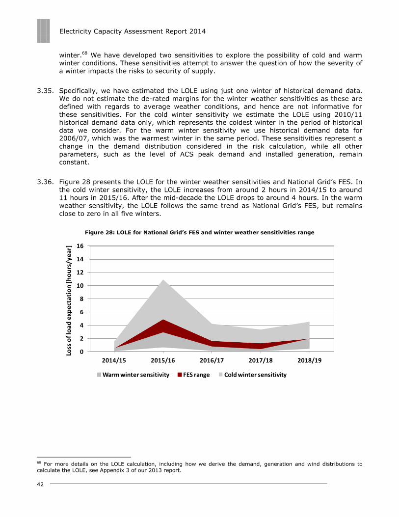
Electricity Capacity Assessment Report 2014
42
winter.68 We have developed two sensitivities to explore the possibility of cold and warm
winter conditions. These sensitivities attempt to answer the question of how the severity of
a winter impacts the risks to security of supply.
3.35. Specifically, we have estimated the LOLE using just one winter of historical demand data.
We do not estimate the de-rated margins for the winter weather sensitivities as these are
defined with regards to average weather conditions, and hence are not informative for
these sensitivities. For the cold winter sensitivity we estimate the LOLE using 2010/11
historical demand data only, which represents the coldest winter in the period of historical
data we consider. For the warm winter sensitivity we use historical demand data for
2006/07, which was the warmest winter in the same period. These sensitivities represent a
change in the demand distribution considered in the risk calculation, while all other
parameters, such as the level of ACS peak demand and installed generation, remain
constant.
3.36. Figure 28 presents the LOLE for the winter weather sensitivities and National Grid’s FES. In
the cold winter sensitivity, the LOLE increases from around 2 hours in 2014/15 to around
11 hours in 2015/16. After the mid-decade the LOLE drops to around 4 hours. In the warm
weather sensitivity, the LOLE follows the same trend as National Grid’s FES, but remains
close to zero in all five winters.
Figure 28: LOLE for National Grid’s FES and winter weather sensitivities range
68 For more details on the LOLE calculation, including how we derive the demand, generation and wind distributions to calculate the LOLE, see Appendix 3 of our 2013 report.
0
2
4
6
8
10
12
14
16
2014/15 2015/16 2016/17 2017/18 2018/19
Loss
of
load
exp
ect
atio
n [
ho
urs
/ye
ar]
Warm winter sensitivity FES range Cold winter sensitivity
Electricity Capacity Assessment Report 2014
43
Appendices
Index
Appendix Name of Appendix Page Number
1 Detailed results tables 44
2 Glossary 55
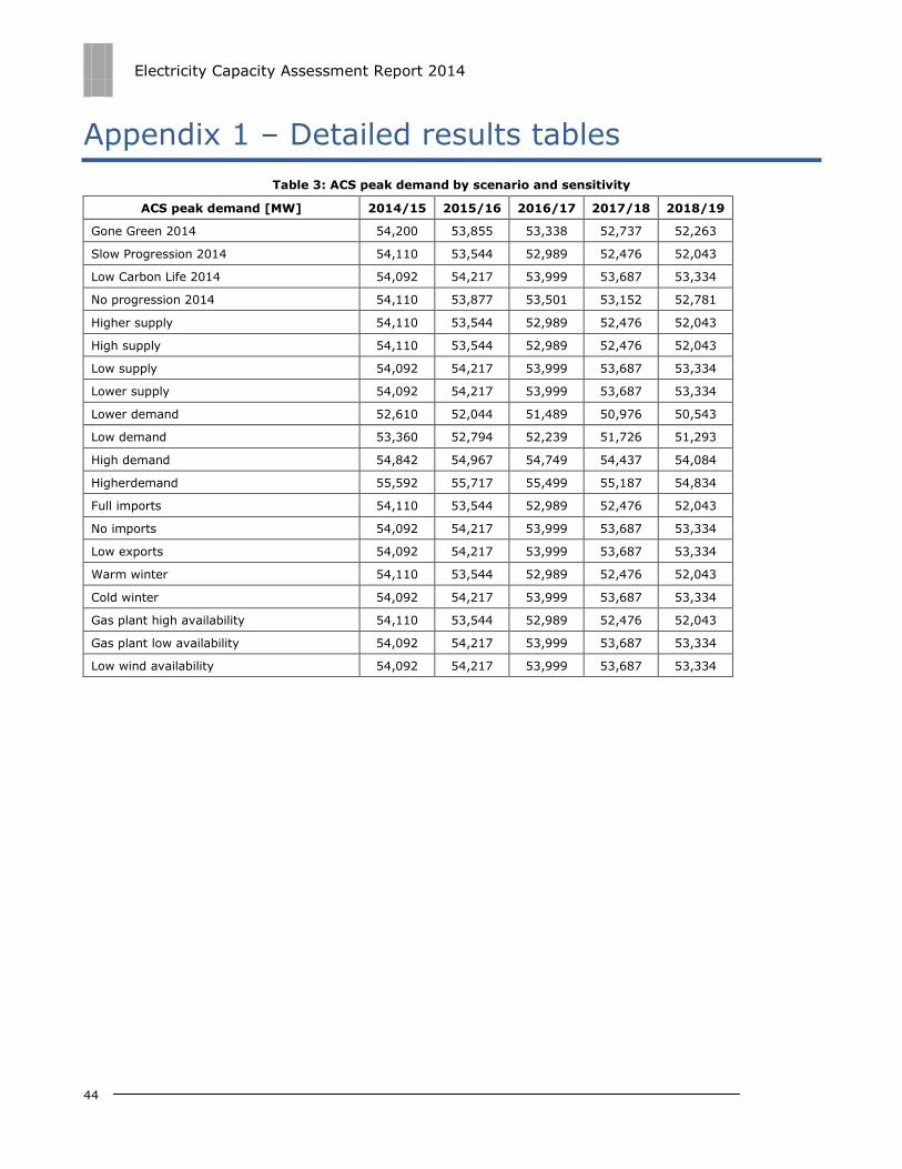
Electricity Capacity Assessment Report 2014
44
Appendix 1 – Detailed results tables
Table 3: ACS peak demand by scenario and sensitivity
ACS peak demand [MW] 2014/15 2015/16 2016/17 2017/18 2018/19
Gone Green 2014 54,200 53,855 53,338 52,737 52,263
Slow Progression 2014 54,110 53,544 52,989 52,476 52,043
Low Carbon Life 2014 54,092 54,217 53,999 53,687 53,334
No progression 2014 54,110 53,877 53,501 53,152 52,781
Higher supply 54,110 53,544 52,989 52,476 52,043
High supply 54,110 53,544 52,989 52,476 52,043
Low supply 54,092 54,217 53,999 53,687 53,334
Lower supply 54,092 54,217 53,999 53,687 53,334
Lower demand 52,610 52,044 51,489 50,976 50,543
Low demand 53,360 52,794 52,239 51,726 51,293
High demand 54,842 54,967 54,749 54,437 54,084
Higherdemand 55,592 55,717 55,499 55,187 54,834
Full imports 54,110 53,544 52,989 52,476 52,043
No imports 54,092 54,217 53,999 53,687 53,334
Low exports 54,092 54,217 53,999 53,687 53,334
Warm winter 54,110 53,544 52,989 52,476 52,043
Cold winter 54,092 54,217 53,999 53,687 53,334
Gas plant high availability 54,110 53,544 52,989 52,476 52,043
Gas plant low availability 54,092 54,217 53,999 53,687 53,334
Low wind availability 54,092 54,217 53,999 53,687 53,334
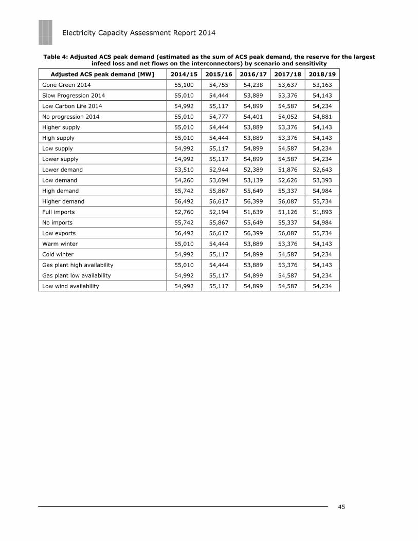
Electricity Capacity Assessment Report 2014
45
Table 4: Adjusted ACS peak demand (estimated as the sum of ACS peak demand, the reserve for the largest infeed loss and net flows on the interconnectors) by scenario and sensitivity
Adjusted ACS peak demand [MW] 2014/15 2015/16 2016/17 2017/18 2018/19
Gone Green 2014 55,100 54,755 54,238 53,637 53,163
Slow Progression 2014 55,010 54,444 53,889 53,376 54,143
Low Carbon Life 2014 54,992 55,117 54,899 54,587 54,234
No progression 2014 55,010 54,777 54,401 54,052 54,881
Higher supply 55,010 54,444 53,889 53,376 54,143
High supply 55,010 54,444 53,889 53,376 54,143
Low supply 54,992 55,117 54,899 54,587 54,234
Lower supply 54,992 55,117 54,899 54,587 54,234
Lower demand 53,510 52,944 52,389 51,876 52,643
Low demand 54,260 53,694 53,139 52,626 53,393
High demand 55,742 55,867 55,649 55,337 54,984
Higher demand 56,492 56,617 56,399 56,087 55,734
Full imports 52,760 52,194 51,639 51,126 51,893
No imports 55,742 55,867 55,649 55,337 54,984
Low exports 56,492 56,617 56,399 56,087 55,734
Warm winter 55,010 54,444 53,889 53,376 54,143
Cold winter 54,992 55,117 54,899 54,587 54,234
Gas plant high availability 55,010 54,444 53,889 53,376 54,143
Gas plant low availability 54,992 55,117 54,899 54,587 54,234
Low wind availability 54,992 55,117 54,899 54,587 54,234
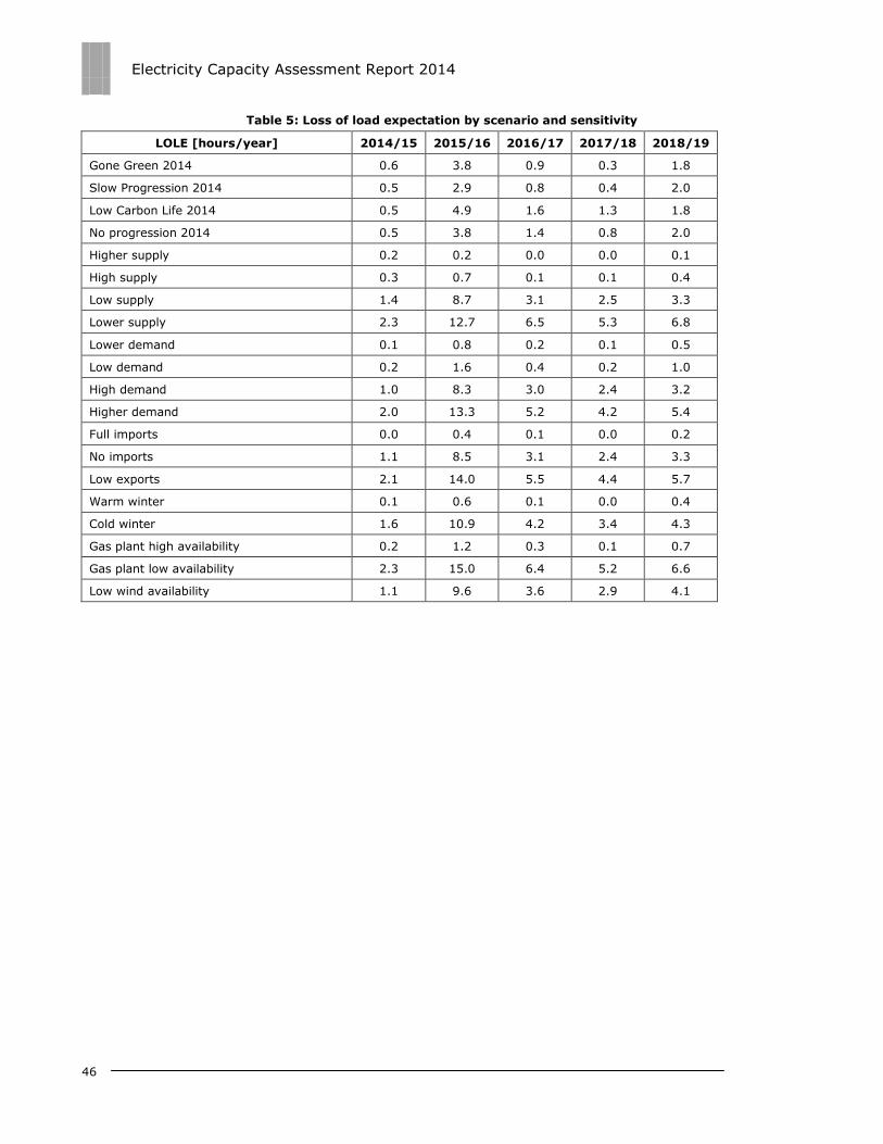
Electricity Capacity Assessment Report 2014
46
Table 5: Loss of load expectation by scenario and sensitivity
LOLE [hours/year] 2014/15 2015/16 2016/17 2017/18 2018/19
Gone Green 2014 0.6 3.8 0.9 0.3 1.8
Slow Progression 2014 0.5 2.9 0.8 0.4 2.0
Low Carbon Life 2014 0.5 4.9 1.6 1.3 1.8
No progression 2014 0.5 3.8 1.4 0.8 2.0
Higher supply 0.2 0.2 0.0 0.0 0.1
High supply 0.3 0.7 0.1 0.1 0.4
Low supply 1.4 8.7 3.1 2.5 3.3
Lower supply 2.3 12.7 6.5 5.3 6.8
Lower demand 0.1 0.8 0.2 0.1 0.5
Low demand 0.2 1.6 0.4 0.2 1.0
High demand 1.0 8.3 3.0 2.4 3.2
Higher demand 2.0 13.3 5.2 4.2 5.4
Full imports 0.0 0.4 0.1 0.0 0.2
No imports 1.1 8.5 3.1 2.4 3.3
Low exports 2.1 14.0 5.5 4.4 5.7
Warm winter 0.1 0.6 0.1 0.0 0.4
Cold winter 1.6 10.9 4.2 3.4 4.3
Gas plant high availability 0.2 1.2 0.3 0.1 0.7
Gas plant low availability 2.3 15.0 6.4 5.2 6.6
Low wind availability 1.1 9.6 3.6 2.9 4.1
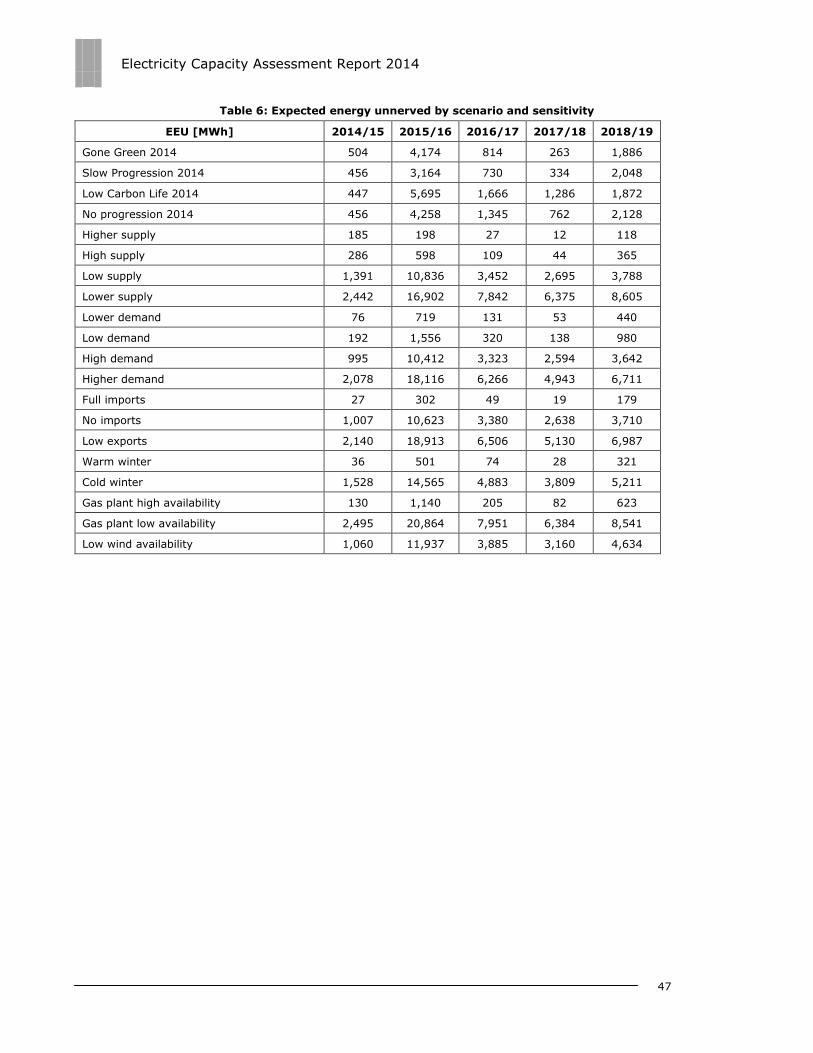
Electricity Capacity Assessment Report 2014
47
Table 6: Expected energy unnerved by scenario and sensitivity
EEU [MWh] 2014/15 2015/16 2016/17 2017/18 2018/19
Gone Green 2014 504 4,174 814 263 1,886
Slow Progression 2014 456 3,164 730 334 2,048
Low Carbon Life 2014 447 5,695 1,666 1,286 1,872
No progression 2014 456 4,258 1,345 762 2,128
Higher supply 185 198 27 12 118
High supply 286 598 109 44 365
Low supply 1,391 10,836 3,452 2,695 3,788
Lower supply 2,442 16,902 7,842 6,375 8,605
Lower demand 76 719 131 53 440
Low demand 192 1,556 320 138 980
High demand 995 10,412 3,323 2,594 3,642
Higher demand 2,078 18,116 6,266 4,943 6,711
Full imports 27 302 49 19 179
No imports 1,007 10,623 3,380 2,638 3,710
Low exports 2,140 18,913 6,506 5,130 6,987
Warm winter 36 501 74 28 321
Cold winter 1,528 14,565 4,883 3,809 5,211
Gas plant high availability 130 1,140 205 82 623
Gas plant low availability 2,495 20,864 7,951 6,384 8,541
Low wind availability 1,060 11,937 3,885 3,160 4,634

Electricity Capacity Assessment Report 2014
48
Table 7: De-rated capacity margin by scenario and sensitivity in MW
De-rated capacity margin [MW] 2014/15 2015/16 2016/17 2017/18 2018/19
Gone Green 2014 3,590 1,707 3,156 4,034 2,396
Slow Progression 2014 3,669 1,966 3,239 3,839 2,390
Low Carbon Life 2014 3,683 1,405 2,553 2,780 2,443
No progression 2014 3,669 1,688 2,731 3,198 2,368
Higher supply 4,393 4,321 5,717 6,229 4,710
High supply 4,043 3,434 4,725 5,333 3,838
Low supply 2,737 746 1,896 2,131 1,810
Lower supply 2,236 262 1,085 1,300 1,003
Lower supply 4,983 3,236 4,521 5,127 3,638
Low demand 4,323 2,598 3,877 4,479 3,010
High demand 3,035 781 1,931 2,168 1,847
Higher demand 2,391 161 1,315 1,562 1,259
Full imports 5,659 3,892 5,185 5,793 4,286
No imports 3,031 777 1,927 2,162 1,841
Low exports 2,381 153 1,305 1,550 1,247
Gas plant high availability 4,406 2,688 3,997 4,617 3,163
Gas plant low availability 2,448 194 1,291 1,536 1,238
Low wind availability 2,961 627 1,771 1,972 1,607

Electricity Capacity Assessment Report 2014
49
Table 8: De-rated capacity margin by scenario and sensitivity in %
De-rated capacity margin [%] 2014/15 2015/16 2016/17 2017/18 2018/19
Gone Green 2014 6.5% 3.1% 5.8% 7.5% 4.5%
Slow Progression 2014 6.7% 3.6% 6.0% 7.2% 4.4%
Low Carbon Life 2014 6.7% 2.5% 4.6% 5.1% 4.5%
No progression 2014 6.7% 3.1% 5.0% 5.9% 4.3%
Higher supply 8.0% 7.9% 10.6% 11.7% 8.7%
High supply 7.4% 6.3% 8.8% 10.0% 7.1%
Low supply 5.0% 1.4% 3.5% 3.9% 3.3%
Lower supply 4.1% 0.5% 2.0% 2.4% 1.8%
Lower demand 9.3% 6.1% 8.6% 9.9% 6.9%
Low demand 8.0% 4.8% 7.3% 8.5% 5.6%
High demand 5.4% 1.4% 3.5% 3.9% 3.4%
Higher demand 4.2% 0.3% 2.3% 2.8% 2.3%
Full imports 10.7% 7.5% 10.0% 11.3% 8.3%
No imports 5.4% 1.4% 3.5% 3.9% 3.3%
Low exports 4.2% 0.3% 2.3% 2.8% 2.2%
Gas plant high availability 8.0% 4.9% 7.4% 8.6% 5.8%
Gas plant low availability 4.5% 0.4% 2.4% 2.8% 2.3%
Low wind availability 5.4% 1.1% 3.2% 3.6% 3.0%
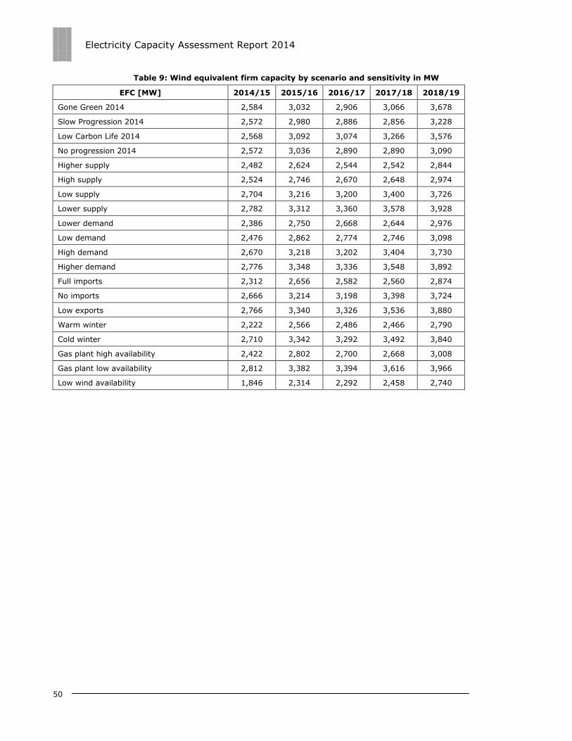
Electricity Capacity Assessment Report 2014
50
Table 9: Wind equivalent firm capacity by scenario and sensitivity in MW
EFC [MW] 2014/15 2015/16 2016/17 2017/18 2018/19
Gone Green 2014 2,584 3,032 2,906 3,066 3,678
Slow Progression 2014 2,572 2,980 2,886 2,856 3,228
Low Carbon Life 2014 2,568 3,092 3,074 3,266 3,576
No progression 2014 2,572 3,036 2,890 2,890 3,090
Higher supply 2,482 2,624 2,544 2,542 2,844
High supply 2,524 2,746 2,670 2,648 2,974
Low supply 2,704 3,216 3,200 3,400 3,726
Lower supply 2,782 3,312 3,360 3,578 3,928
Lower demand 2,386 2,750 2,668 2,644 2,976
Low demand 2,476 2,862 2,774 2,746 3,098
High demand 2,670 3,218 3,202 3,404 3,730
Higher demand 2,776 3,348 3,336 3,548 3,892
Full imports 2,312 2,656 2,582 2,560 2,874
No imports 2,666 3,214 3,198 3,398 3,724
Low exports 2,766 3,340 3,326 3,536 3,880
Warm winter 2,222 2,566 2,486 2,466 2,790
Cold winter 2,710 3,342 3,292 3,492 3,840
Gas plant high availability 2,422 2,802 2,700 2,668 3,008
Gas plant low availability 2,812 3,382 3,394 3,616 3,966
Low wind availability 1,846 2,314 2,292 2,458 2,740
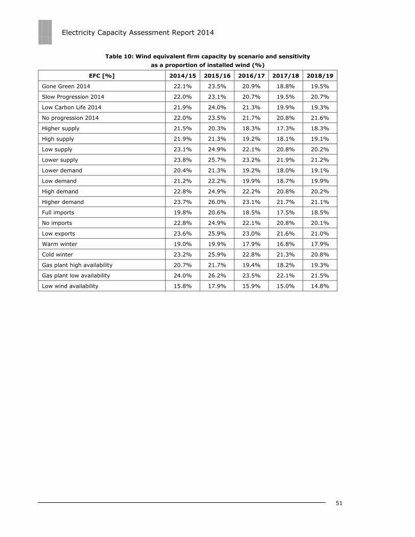
Electricity Capacity Assessment Report 2014
51
Table 10: Wind equivalent firm capacity by scenario and sensitivity
as a proportion of installed wind (%)
EFC [%] 2014/15 2015/16 2016/17 2017/18 2018/19
Gone Green 2014 22.1% 23.5% 20.9% 18.8% 19.5%
Slow Progression 2014 22.0% 23.1% 20.7% 19.5% 20.7%
Low Carbon Life 2014 21.9% 24.0% 21.3% 19.9% 19.3%
No progression 2014 22.0% 23.5% 21.7% 20.8% 21.6%
Higher supply 21.5% 20.3% 18.3% 17.3% 18.3%
High supply 21.9% 21.3% 19.2% 18.1% 19.1%
Low supply 23.1% 24.9% 22.1% 20.8% 20.2%
Lower supply 23.8% 25.7% 23.2% 21.9% 21.2%
Lower demand 20.4% 21.3% 19.2% 18.0% 19.1%
Low demand 21.2% 22.2% 19.9% 18.7% 19.9%
High demand 22.8% 24.9% 22.2% 20.8% 20.2%
Higher demand 23.7% 26.0% 23.1% 21.7% 21.1%
Full imports 19.8% 20.6% 18.5% 17.5% 18.5%
No imports 22.8% 24.9% 22.1% 20.8% 20.1%
Low exports 23.6% 25.9% 23.0% 21.6% 21.0%
Warm winter 19.0% 19.9% 17.9% 16.8% 17.9%
Cold winter 23.2% 25.9% 22.8% 21.3% 20.8%
Gas plant high availability 20.7% 21.7% 19.4% 18.2% 19.3%
Gas plant low availability 24.0% 26.2% 23.5% 22.1% 21.5%
Low wind availability 15.8% 17.9% 15.9% 15.0% 14.8%
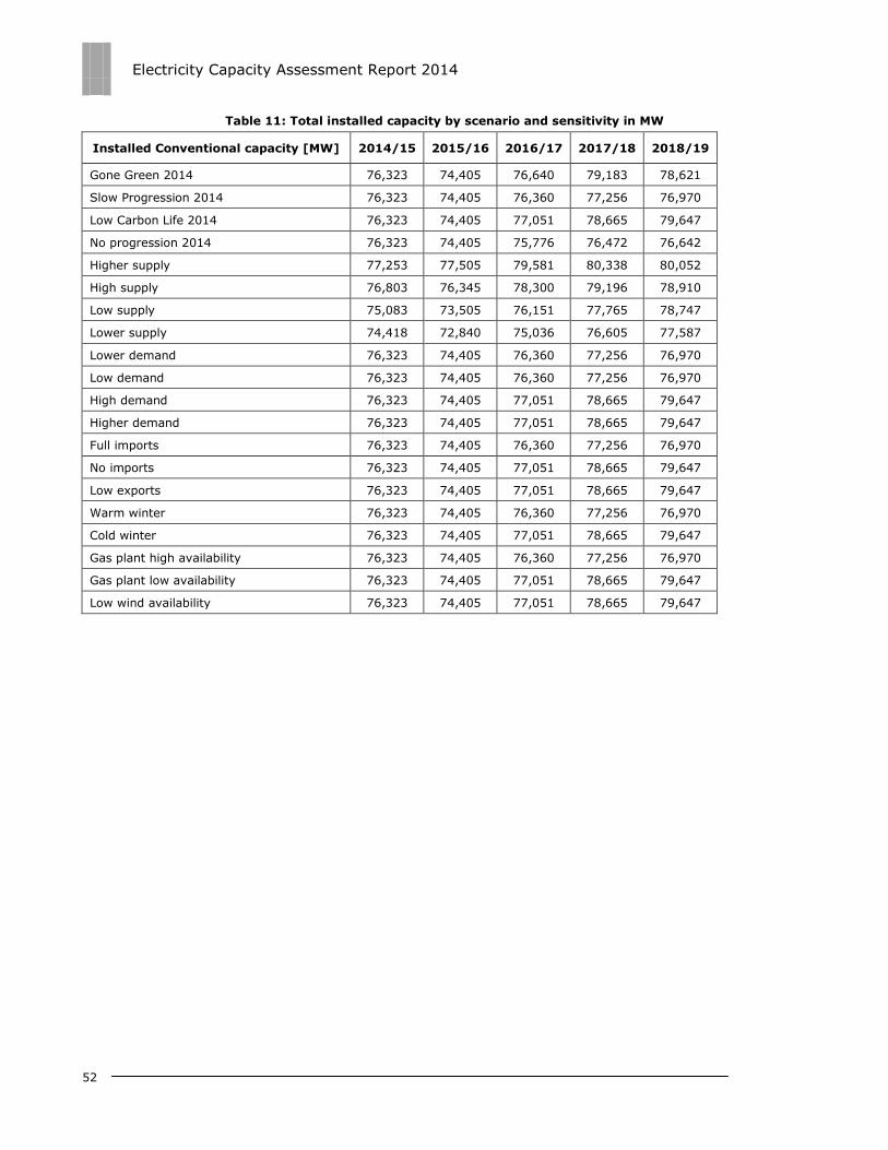
Electricity Capacity Assessment Report 2014
52
Table 11: Total installed capacity by scenario and sensitivity in MW
Installed Conventional capacity [MW] 2014/15 2015/16 2016/17 2017/18 2018/19
Gone Green 2014 76,323 74,405 76,640 79,183 78,621
Slow Progression 2014 76,323 74,405 76,360 77,256 76,970
Low Carbon Life 2014 76,323 74,405 77,051 78,665 79,647
No progression 2014 76,323 74,405 75,776 76,472 76,642
Higher supply 77,253 77,505 79,581 80,338 80,052
High supply 76,803 76,345 78,300 79,196 78,910
Low supply 75,083 73,505 76,151 77,765 78,747
Lower supply 74,418 72,840 75,036 76,605 77,587
Lower demand 76,323 74,405 76,360 77,256 76,970
Low demand 76,323 74,405 76,360 77,256 76,970
High demand 76,323 74,405 77,051 78,665 79,647
Higher demand 76,323 74,405 77,051 78,665 79,647
Full imports 76,323 74,405 76,360 77,256 76,970
No imports 76,323 74,405 77,051 78,665 79,647
Low exports 76,323 74,405 77,051 78,665 79,647
Warm winter 76,323 74,405 76,360 77,256 76,970
Cold winter 76,323 74,405 77,051 78,665 79,647
Gas plant high availability 76,323 74,405 76,360 77,256 76,970
Gas plant low availability 76,323 74,405 77,051 78,665 79,647
Low wind availability 76,323 74,405 77,051 78,665 79,647

Electricity Capacity Assessment Report 2014
53
Table 12: Total conventional installed capacity by scenario and sensitivity in MW
Installed Conventional capacity [MW] 2014/15 2015/16 2016/17 2017/18 2018/19
Gone Green 2014 64,618 61,505 62,721 62,870 59,777
Slow Progression 2014 64,618 61,505 62,441 62,590 61,404
Low Carbon Life 2014 64,618 61,505 62,596 62,293 61,161
No progression 2014 64,618 61,505 62,441 62,590 62,368
Higher supply 65,548 64,605 65,662 65,672 64,486
High supply 65,098 63,445 64,381 64,530 63,344
Low supply 63,378 60,605 61,696 61,393 60,261
Lower supply 62,713 59,940 60,581 60,233 59,101
Lower demand 64,618 61,505 62,441 62,590 61,404
Low demand 64,618 61,505 62,441 62,590 61,404
High demand 64,618 61,505 62,596 62,293 61,161
Higher demand 64,618 61,505 62,596 62,293 61,161
Full imports 64,618 61,505 62,441 62,590 61,404
No imports 64,618 61,505 62,596 62,293 61,161
Low exports 64,618 61,505 62,596 62,293 61,161
Warm winter 64,618 61,505 62,441 62,590 61,404
Cold winter 64,618 61,505 62,596 62,293 61,161
Gas plant high availability 64,618 61,505 62,441 62,590 61,404
Gas plant low availability 64,618 61,505 62,596 62,293 61,161
Low wind availability 64,618 61,505 62,596 62,293 61,161
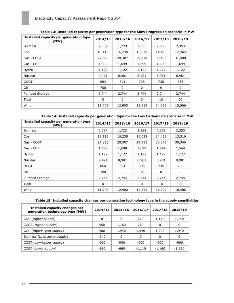
Electricity Capacity Assessment Report 2014
54
Table 13: Installed capacity per generation type for the Slow Progression scenario in MW
Installed capacity per generation type [MW]
2014/15 2015/16 2016/17 2017/18 2018/19
Biomass 2,037 1,723 2,353 2,353 2,353
Coal 18,116 16,238 15,029 14,458 12,342
Gas - CCGT 27,865 28,307 29,778 30,488 31,408
Gas - CHP 1,699 1,699 1,699 1,699 1,699
Hydro 1,122 1,122 1,122 1,122 1,122
Nuclear 9,471 8,981 8,981 8,981 8,981
OCGT 864 691 735 735 735
Oil 700 0 0 0 0
Pumped Storage 2,744 2,744 2,744 2,744 2,744
Tidal 0 0 0 10 20
Wind 11,705 12,900 13,919 14,666 15,566
Table 14: Installed capacity per generation type for the Low Carbon Life scenario in MW
Installed capacity per generation type [MW]
2014/15 2015/16 2016/17 2017/18 2018/19
Biomass 2,037 1,723 2,353 2,353 2,353
Coal 18,116 16,238 15,029 14,458 13,316
Gas - CCGT 27,865 28,307 29,933 30,346 30,346
Gas - CHP 1,699 1,699 1,699 1,544 1,544
Hydro 1,122 1,122 1,122 1,122 1,122
Nuclear 9,471 8,981 8,981 8,981 8,981
OCGT 864 691 735 735 735
Oil 700 0 0 0 0
Pumped Storage 2,744 2,744 2,744 2,744 2,744
Tidal 0 0 0 10 20
Wind 11,705 12,900 14,455 16,372 18,486
Table 15: Installed capacity changes per generation technology type in the supply sensitivities
Installed capacity changes per generation technology type [MW]
2014/15 2015/16 2016/17 2017/18 2018/19
Coal (Higher supply) 0 0 570 1,140 1,140
CCGT (Higher supply) 450 1,160 710 0 0
Coal (High/Higher supply) 480 1,940 1,940 1,940 1,940
Biomass (Low/Lower supply) -340 0 0 0 0
CCGT (Low/Lower supply) -900 -900 -900 -900 -900
CCGT (Lower supply) -660 -660 -1,110 -1,160 -1,160
Electricity Capacity Assessment Report 2014
55
Appendix 2 - Glossary
A
ACS
Average Cold Spell. This is a weather-independent measure of the underlying level of demand in a
winter.
C
Capacity margin
The capacity margin is defined as the excess of installed generation over demand. It is sometimes
referred to as reserve margin.
Capacity market (capacity mechanism)
Policy instrument designed to help ensure security of supply by providing a more secure capacity
margin than that which would be determined by the market without intervention.
Carbon Price Floor
The carbon price floor is a tax on fossil fuels used in the generation of electricity. This is achieved
through changes to the existing Climate Change Levy (CCL) regime in the case of gas, solid fuels
and liquefied petroleum gas (LPG) used in electricity generation. These changes include the
setting up of new carbon price support (CPS) rates of CCL.
Combined Cycle Gas Turbine (CCGT)
A power station that generates electricity by means of a number of gas turbines whose exhaust is
used to make steam to generate additional electricity via a steam turbine, thereby increasing the
efficiency of the plant above open cycle gas turbines.
Combined Heat and Power (CHP)
The simultaneous generation of usable heat and power (usually electricity) in a single process,
thereby leading to reductions in the amount of wasted heat.
Constraints (also known as congestion)
A constraint occurs when the capacity of transmission assets is exceeded so that not all of the
required generation can be transmitted to other parts of the network, or an area of demand
cannot be supplied with all of the required generation.

Electricity Capacity Assessment Report 2014
56
Consumer
In considering consumers in the regulatory framework we consider users of network services (for
example generators, shippers) as well as domestic and business end consumers, and their
representatives.
D
DECC
Department of Energy and Climate Change.
Demand-side Response (DSR)
An active, short term reduction in electricity consumption either through shifting it to another
period, using another type of generation, or simply not using electricity at that time.
De-rated capacity margin
The de-rated capacity margin is defined as the average excess of available generation capacity
over peak demand, expressed in percentage terms. Available generation capacity takes into
account the contribution of installed capacity at peak demand by adjusting it by the appropriate
de-rating (or availability) factors which take into account the fact that plant are sometimes
unavailable due to outages.
Distribution Network
The system of electric lines that carry electricity from the high voltage transmission grid and
distribute it over low voltage networks to industrial, commercial, and domestic users.
E
Embedded generation
Any generation which is connected directly to the local distribution network, as opposed to the
transmission network, as well as combined heat and power schemes of any scale. The electricity
generated by such schemes is typically used in the local system rather than being transported
across the UK.
EMR
Electricity Market Reform.
Energy efficiency
A change in the use of energy to reduce waste and lower energy use. For example, insulation in
buildings, reducing demand from heat, or increasing the efficiency of appliances so they use less
energy.
Electricity Capacity Assessment Report 2014
57
Equivalent firm capacity (EFC)
The quantity of firm capacity (ie always available) that can be replaced by a certain volume of
wind generation to give the same level of security of supply, as measured by LOLE. This measure
is used to calculate the average contribution of wind power to the de-rated margin. It varies with
the proportion of wind power in the system.
Expected energy unserved
The mean (average) amount of electricity demand that is not met in a year. EEU combines both
the likelihood and the potential size of any supply shortfall.
G
GB
Great Britain.
Gigawatt (GW)
The gigawatt is equal to one billion watts (ie 1 gigawatt = 1,000,000,000 watts). The watt
symbol: W) is a derived unit of power in the International System of Units. Power is the rate at
which energy is generated or consumed and hence is measured in units (eg watts) that represent
“energy transfered per unit time”.
I
IFA
Interconnexion France Angleterre. The England to France Interconnector is a 2,000MW high
voltage direct current (HVDC) link between the French and British transmission systems with
ownership shared between National Grid and Réseau de Transport d'Electricité (RTE).
Interconnector
Electricity interconnectors are electric lines or other electrical plants based within the jurisdiction
of Great Britain that convey electricity (whether in both directions or in only one) between Great
Britain and another country or territory.
Intermittent generation
Electricity generation technology that produces electricity at irregular and, to an extent,
unpredictable intervals, eg wind turbines.

Electricity Capacity Assessment Report 2014
58
L
Largest infeed loss (or reserve requirement)
A reserve of power that National Grid as System Operator reserves to maintain system frequency
in the event of the loss of the largest generator. Currently the National Electricity Transmission
System Security Quality of Supply Standards limits the largest infeed loss reserve to 1.8GW, as of
April 2014.
Loss of Load Expectation (LOLE)
The mean (average) number of hours per year in which supply does not meet demand in the
absence of intervention from the System Operator.
M
Megawatt (MW)
The megawatt is equal to one million watts (ie 1 megawatt = 1,000,000 watts). The watt symbol:
W) is a derived unit of power in the International System of Units. Power is the rate at which
energy is generated or consumed and hence is measured in units (eg watts) that represent
“energy transferred per unit time”.
Mothballed
A term often used for long term storage of Generating Units. Such plant is sometimes also
referred to as “decommissioned”.
N
National Grid or National Grid Electricity Transmission plc (NGET)
National Grid is the Transmission System Operator for Great Britain. As part of this role it is
responsible for procuring balancing services to balance demand and supply and to ensure the
security and quality of electricity supply across the Great Britain Transmission System.
NI
Northern Ireland.
O
Outages
The shutdown of a generating unit, transmission line, or other facility for emergency reasons or a
condition in which the generating equipment is unavailable for load due to technical (unexpected)
or strategic reasons.

Electricity Capacity Assessment Report 2014
59
Ofgem/The Authority
Ofgem is the Office of Gas and Electricity Markets, which supports the Gas and Electricity Markets
Authority (“the Authority”), the regulator of the gas and electricity industries in Great Britain.
P
Peak demand, peak load
These two terms are used interchangeably to denote the maximum power requirement of a
system at a given time, or the amount of power required to supply customers at times when need
is greatest. They can refer either to the load at a given moment (eg a specific time of day) or to
averaged load over a given period of time (eg a specific day or hour of the day).
Pumped storage
The process, also known as hydroelectric storage, for converting large quantities of electrical
energy to potential energy by pumping water to a higher elevation, where it can be stored
indefinitely and then released to pass through hydraulic turbines and generate electrical energy.
R
Reliability standard
The standard set by the Government for the level of security of supply of the GB national
electricity system. It is set at three hours of loss of load expectation in any delivery year
S
Scheduled outage
The shutdown of a generating unit, transmission line, or other facility for inspection or
maintenance, in accordance with an advance schedule.
Sensitivity
This is a test whereby a single factor is changed (eg interconnector flows) holding all other factors
fixed to their base case value to see the effect the single factor produces on the model output (eg
on LOLE).
System Operator (SO)
The entity responsible for operating the GB electricity transmission system and for entering into
contracts with those who want to connect to and/or use the electricity transmission system.
National Grid is the GB electricity transmission system operator.
Electricity Capacity Assessment Report 2014
60
T
Transmission Losses
Electricity lost on the Great Britain transmission system through the physical process of
transporting electricity across the network.
Transmission System
The system of high voltage electric lines providing for the bulk transfer of electricity across GB.