electrical resistivity in tuffs
TRANSCRIPT

ELECTRICAL RESISTIVITY CHANGES
by
Carolyn Alexandria Morrow
S.B., Massachusetts Institute of Technology
(1978)
SUBMITTED IN PARTIAL FULFILLMENT
OF THE REQUIREMENTS FOR THE
DEGREE OF
MASTER OF SCIENCE
at the
MASSACHUSETTS INSTITUTE OF TECHNOLOGY
September, 1979
Signature of Author...... ...... . ........ .... ..
Department of Ea th and Planetary Sciences,September, 1979
Certified by.. . . . . . . . . . . . . ........ ,.. .. ..Thesis Supervisor
Accepted by . . . . . . . . . . . . . . . . . . . . . . . .Chairman, Depar tment Committee on Graduate Students
3)- H CHNLGY
MIT LIBRAR- i
IN TUFFS

ABSTRACT
ELECTRICAL RESISTIVITY CHANGES IN TUFFS
by
Carolyn Alexandria Morrow
Submitted to the Department of Earth and PlanetarySciences on August 28 , 1979 in partial fulfillment of therequirements for the degree of Master of Science.
Samples of northern California tuffs were stressedwhile simultaneously measuring electrical resistance changesto investigate a phenomenon observed by Yanazaki on similarrocks from Japan. Resistance decreased substantially at lowstrain values for partially saturated samples. Strain wasamplified between 103 and 105 by the associated change inelectrical resistance.
The process was repeatable and recoverable in the tuffsunlike the behavior of other rock types. The principalfactors involved were porosity, Young's modulus and degreeof saturation.
A method is described to quickly sort out theelectrically amplifying tuffs from those that are not, as afirst step in locating a field site where this phenomenoncould be used as an earthquake monitoring technique.
Thesis Supervisor: William F. BraceProfessor of Geology

TABLE OF CONTENTS
LIST OF FIGURES . . . . .
LIST OF TABLES. . . . . .
ACKNOWLEDGMENTS . . . . .
CHAPTER I Introduction
II Rocks Studied.
Sampling. .
Rock Descrip
III Experimental Pr
IV Observations .
Stress-Strai
Electrical C
V Discussion . .
Amplificatio
Recoverabili
VI Conclusions. .
APPENDIX A
APPENDIX B
APPENDIX C
APPENDIX Dl
D2
Studies of Neva
The Chunk Test
. . . . . . . . . 0 . . . . . 4
. 0 0 0 0 0 0 0 0 7
. 0 . 0 . 0 0 0 0 . 0 . 0 . 11
. . . . . 0 0 . . . . . . . . 11
tions . . . . . . . . . . . . 13
ocedure . . . . . . . . . . . 17
. . .. . . . . . . . . 20
n Behavior. . .. . . . . . . 20
hanges with Stress. . . . . . 23
36
n Factor. . . . . . . . . . . 36
ty. . Montana .uffs. . . . . 38
. . 40
da and Montana Tuffs. . . 41
. 0 . 0 0 .o e . . . . 55
Stress-Strain and Electrical Behavior
Selected California Tuffs . . .
Resistance Measuring Techniques. . .
Choice of Electrode Material . . . .
. . . . 65
. . . . 74
. . . . 86
D3 Frequency Effects. . . . . * . . . 0 0 .
REFERENCES. . . . 0 ~ ~ ~ 0 0 ~ ~ 0 0 ~ ~ ~ ~ . . . 0
-3-
. . 89
. . 93

LIST OF FIGURES
CHAPTER III
Figure 3.1 Experimental apparatus. . . . . . . . . . 19
CHAPTER IV
Figure 4.1
Figure 4.2
Typical stress-strain curves,GPT and DPR. . . . . . . . . . .
Young's modulus of tuff samplesversus porosity. . . . . . . . . .
Figure 4.3 Change in electrical resistance withstress of the Grizzly Peak tuffand Berea sandstone. . . . . . . .
Figure 4.4 Relative change in resistivity withstrain, SIL. . . . . . . . . .
. . 21
. . 22
. . 26
. . 27
Figure 4.5
Figure 4.6
Figure 4.7
Figure 4.8
Figure 4.9
Amplification factor versus saturationof the California tuffs. . . . . .
Relation of Young's modulus tosaturation at maximum amplification(peak saturation). . . . . . . . . .
Porosity of tuffs versuspeak saturation. . . . . . . . . . .
Maximum amplification of tuff samplesversus porosity. . . . . . . . . . .
Maximum amplification of tuffs versuspeak saturation. . . . . . . . . . .
Appendix A
Figure Al
Figure A2
Figure A3
Figure A4
Stress-strain curves of Nevada/Montanatuffs and the Pottsville dnd Bereasandstone. . . . . . . . . . . . .
Change in resistance with sta ass:Tunnel Beds tuff and BereE sandstone
Change in resistance with stress:Pottsville, Navajo and Mixed Company(Kayenta) sandstones . . .. . . . .
Relative change in resistivity withstrain, Butte Lapilli tuff . . . . .
-4-
28
29
30
31
32
. 46
. 47
. 48
. 49

Figure A5 Relative change in resistivity withstrain, Berea sandstone. . . . . . .
Appendix B
Figure Bl
Figure B2
Figure B3
Figure B4
Figure B5
Sample configuration of the chunk test.
Chunk test experimental apparatus
Change in resistance with stress:SHR, DPR, RLS, DRY . . . . . .
Change in resistance with stress:MWT, SZT, GPT. . . . . . . . .
Change in resistance with stress:SJB, SIL, RTT, COT . . . . . .
. 60
. . . . 60
. . . .. 61
. . . . 62
. . . . 63
Appendix C
Figure Cl
Figure C2
Figure C3
Figure C4
Figure C5
Figure C6
Figure C7
Figure C8
Appendix D
Figure Dl
Figure D2
Stress-strain relation for theCalifornia tuffs . . . . . . . . . . . 66
Change in resistance with stress:GPT, SIL, SHR. . . . . . . . . . . . . 67
Change in resistance with stress:DPR, SZT, RTT. . . . . . . . . . . . . 68
Relative change in resistivity withstrain, GPT. . . . * . . . . . . . . . 69
Relative change in resistivity withstrain, SHR. . . . . . . . . . . . . . 70
Relative change in resistivity withstrain, SZT. . . . . .... ...... . 71
Relative change in resistivity withstrain, DPR. . . . . . . . . . . . . . 72
Relative change in resistivity withstrain, RTT. . . . . . . . * . . . . . 73
Stress effect of various electrodes,20 kilohm resistor at 10 Hz. . . .
Resistance fall-off with frequency forthe California tuffs at varyingsaturations. . . . . . . . . . . .
. . 88
. 92
0 50

LIST OF TABLES
Table 2.1
Table 4.1
-Table 4.2
Table Al
Table A2
Table A3
Table Bl
Table B2
Rock Descriptions of Selected CaliforniaTuffs. . . . . . . . . . . . . . . . .
Strain Amplification of the CaliforniaTuffs. . . . . * . * . * . . . . .
Physical Properties of the CaliforniaTuffs. . . . . . . . . . . . . . . . .
Rock Descriptions and Locations of theMontana/Nevada Tuffs and Sandstones. .
Strain Amplification of the Montana/NevadaTuffs. . . . . . . . . . . . . . . . . .
Strain Amplification of Sandstones. . .
Location and Hand Specimen Descriptionsof the California Tuffs. . . . . . .
Relative Ordering of Electrical Propertiesof California Tuffs. . . . . . . . . . .
-6-
15
. 33
. 35
. 44
. 51
. 53
. 58
. 64

ACKNOWLEDGMENTS
I would like to thank William F. Brace for his support
and advice throughout this work. Charles Chesterman of the
California Bureau of Mines and Garniss Curtis of the
University of California at Berkeley aided in the location
and collection of samples. Michael Coln was very helpful in
improving the electrical measuring techniques, and in typing
this thesis.
-7-
CHAPTER I
Introduction
In 1965 Yamazaki called attention to dramatic
electrical resistivity changes thought to be caused by earth
tides. Resistivity variations a thousand times larger than
the tidal strain were recorded in a cave near Tokyo, Japan.
Although the tidal origin is still disputed Madden, [1978],
Yamazaki subsequently confirmed in the laboratory [1965,
1966] the unusual electrical sensitivity to strain of the
particular tuffaceous rocks where the field observations
were first made. Others have shown that resistivity of
rocks changes with stress (Parkhomenko [1967], Brace and
Orange [19631, for example), but generally the changes were
but a small fraction of those noted by Yamazaki,
particularly in porous rocks [Brace 1974].
The electrical effects reported by Yamazaki were
limited to tuffaceous rocks, partially saturated and at very
low stresses. Because of the potential application to
crustal deformation studies or to earthquake prediction
(Rikitake and Yamazaki [1969]), it seemed worthwhile to
extend his work, not only to other rocks, but to a wider
range of conditions. Tuffaceous sandstone showed a weaker
effect than lapilli tuff [Yamazaki 1966]. Would other
sandstones be similar? What is the optimum mineralogy,
-.8-

porosity, saturation and stress level? Do appropriate rocks
exist near active fault zones in the United States? Even if
they do not, the mechanism of this fascinating effect needs
to be explained. How can resistivity in a partially
saturated highly porous rock change so dramatically in a
reversible way?
To explore such questions, a laboratory experiment was
designed which would attain the conditions of stress,
saturation and would include rock types similar to those
studied by Yamazaki. Since the field site was located in a
tuff cave with electrodes affixed to the floor and walls, an
unconfined compression test best approximated the in situ
stress state. In the compression tests, stress, strain and
electrical resistance were simultaneously measured to a
maximum stress of 6 MPa. This stress was chosen to avoid
permanent damage to the weak tuffs and sardstones studied.
A low stress cycle would ensure repeatable elastic behavior
and perhaps simulate tidal earth loads and certain tectonic
stresses.
Research was carried out in four c'stinct phases.
These were: a) a study of the electrica l properties of
sandstones and tuffs from Nevada and Montana to verify and
further investigate Yamazaki's findings. Preliminary
results were very promising, but the details were vaguely
-9-

understood. Nevertheless, the next step was b) sample
collection of tuffs near active California faults, since a
major goal was the location of sites in the United States
where tuffs could be used in earthquake prediction. Then c)
a rapid approximate method was devised to find which of the
California rocks had more pronounced electrical properties,
and d) several of these tuffs were investigated in detail
under a more complete range of saturations to answer some of
the basic questions mentioned above.
Due to the more comprehensive nature of the California
study, these results are presented as the principal text of
this thesis. The work on sandstones and the Nevada/Montana
tuffs are described in Appendix A. There are a few places
where these data are included with the results of the
California rocks, particularly for completeness and
comparison of rock types. These spots are noted and
referenced.
- 1-0-

CHAPTER II
Rocks Studied
Sampling
With the help of state maps and local geologists,
several tuff sites were located in norther California. The
principal locations were (a) volcanics of the Pinnacles
National Monument, adjacent to the San Andreas fault, (b)
the Berkeley Hills volcanics, next to the Hayward fault, and
(c) the Napa, Somona and Cotati valleys, which are cut by
several lesser faults. In many of these areas, a number of
distinctive tuff deposits are exposed, each of which was
sampled. Sampling was conducted in the dry season (July),
from fresh surface outcrops, with care taken to preserve
natural water content.
With the large number of samples involved, (from over a
dozen sites), it was impossible to do a detailed study of
each locality. Therefore a quick test was devised to sort
out the more electrically sensitive rocks. This was called
the "chunk test", in reference to the hand specimen size
chunks of rocks used rather than machined samples. The
intent of the test was not to produce accurate quantitative
data, but quickly order the rocks in terms of electrical
properties. Details are described in Appendix B. From the
-1-1-

results of the chunk tests, six tuffs from the Berkeley
Hills and Napa valley were chosen for more thorough study
(Table 2.1). A sandstone (Berea) is also included in the
table. Detailed results of other sandstones can be found in
Appendix A.
-12-

Rock Descriptions
Tuffs are the products of explosive volcanic eruptions.
Ash, crystals, glass and rock fragments consolidate into a
porous rock. Carossi [1960] gives a comprehensive
description of tuff petrology and vitroclastic texture.
The six tuffs listed in Table 2.1 represent the three
general catagories of tuffs. SZT and RTT are lithic tuffs,
composed mostly of rock fragments welded together by a
tuffaceous matrix. GPT and DPR fall into the catagory of
.crystal tuffs, which contain a large percentage of
phenocrysts. Finally, SHR and SIL are vitric tuffs,
composed mostly of fine-grained glassy groundmass.
In the descriptions of Table 2.1 (as seen in thin
section), the amount of breakdown of the unstable glass to
clay minerals and zeolites was estimated, as Lhese samples
were not analyzed by X-ray techniques.
Study of fresh fracture surfaces with the scanning
electron microscope revealed a wide range of internal
structures, reflecting tuff type. The glassy specimens,
with little recrystallization of the groundmass had numerous
very small pores (0.5 microns) caused by gas bubbles. SIL
was the most notable example of this type. With increasing
-13-

recrystallization, pores and passageways evidently became
larger, to a maximum of around 50 microns, although precise
determination of pore size, glass content and mineral phases
was difficult from fracture surface micrographs. An attempt
was made to study pore geometry from polished surfaces using
-the ion thinning technique described in Sprunt and Brace
[1974]. These results were largely unsuccessful as the
tuffs were very soft and did not thin uniformly.
-14-

Rock DescriptionsCalifornia Tuffs
Sample Location Porosity(%)
Young'sMod., GPa
of Selected
Description
DPR Deer Park Rd.St. Helena,Napa County
SHR St. HelenaRoad.,Sonoma Co.
SZT SiestaFormationzeolite tuffBerkeley Hills
17.9
37.2
17.1
RTT Round Top Hill 3.7Berkeley Hills
GPT Grizzly PeakBerkeley Hills
3.5
2.2
3.3
12.5
10.010.7
-15-
20% plagioclase andsanidine phenocrysts80% fine grainreworked groundmass,welded banding andflow textures
10% phenocrystsincluding:
8% plagioclase2% fractured quartz
X % lithic fragments90% groundmass:
30% glassy lenses& shard structures30% recrystallizedradial zeolites30% fine grainedgroundmass
80% basaltic lithicfragments5% plagioclase- veryfractured15% zeolitized matrix
60% basalt fragments5% crystalline quartzX % zeolitizedplagioclase35% reworked glass,clay and zeolites
30% pnenocrysts:-.ngul .r fragments,varie~1le size,inclu es:
20% plagioclase5% ,uartzfew % biotite
10% lithic fragments60% groundmass,including iron richmontmorillonite,isolated areas ofbanded texture
Table 2.1

Sample Location Porosity* Young's(%) Mod., GPa
SilveradoTrail, NapaCounty
Bereasandstone
35.6
Ohio, 17.2W. Virginia
2.4
6.5
Description
65% glass30% pumice fragmentsfew % quartz andplagioclase
phenocrysts
Orthoquartzite:95% quartz & chert5% feldspar
*Porosities were determined using the immersion methoddescribed in Brace, Orange and Madden [1965].
-16-
SIL

CHAPTER III
Experimental Procedure
Rock samples were machined into cylindrical cores 2.5
cm in diameter by 5 cm long. BLH strain gauges
(FA-50-12-S6), oriented along the cylindrical axis, recorded
linear strain. An oil pressure piston device was used to
stress the samples in unconfined uniaxial compression up to
an axial stress of 6 MPa as shown schematically in Figure
3.1. Lead electrode sheets, 1.3 mm -in thickness were
attached to either end of the sample to form one side of a
Wheatstone bridge. A detailed description of resistance
measurement techniques can be found in Appendix D. The
sample and electrodes were insulated from the piston and
load cell by a 0.1 mm layer of Pallflex teflon.
Electrical resistance measurements were taken at stress
levels of 0, 0.2, 0.5, 1, 2, 4, and 6 MPa for both
increasing and decreasing stresses. Sampling was more
frequent at the lower stresses as the most change was
expected when the sample first began to strain. In all
cases a source voltage across the rock of 10 Hz AC was used
to minimize the frequency effects due to rock capacitance at
high resistance values.
-17-
The pore fluid used was 35 ohm-meter tap water.
Saturation level was determined by averaging the weights of
the sample both before and after each run. For low
saturation, the variation was at most 1 percent, for higher
saturation it reached 5 percent. Stress and strain
measurements were accurate to 5 percent. The absolute
resistance was known to 20 percent, and relative changes in
resistance were accurate to 5 percent.
-18-

piston
leadteflonbaL I
Figure 3.1 Experimental Apparatus

CHAPTER IV
Observations
Stress-Strain Behavior
Stress-strain behavior in tuffs was highly dependent on
porosity, previous stress history and time factors. Some
samples showed a permanent change in the first stress cycle,
as either a permanent strain or an increase in the modulus.
Succeeding cycles were all nearly identical and fairly
linear on loading and unloading (Figure 4.la). Other
samples were less recoverable and also changed with time
after a loading cycle, as seen for instance with DPR (Figure
4.1b). On the left is the initial trace. Then, immediately
after the first stress cycle, the sample had become stiffer
(center trace). The trace on the right was taken several
days later when the sample had relaxed. The stress-strain
curves for sandstone were similar in shape to those of DPR.
Young's modulus was closely related to porosity (Figure
4.2); the more porous rocks tended to be less stiff.
-20-

DPR
10~
4.la LINEAR STRAIN 4.lb
Figure 4.1 Typical stress-strain curves, GPT and
a.
CnU)wcrI-Cn
GPT
DPR

RTT
GPT
SZT DPI
SHR
20 30
POROSITY,
Figure 4. Young's Modulus of tuff
samples vs. porosity
-22-
1[30
0
0
z0
40 50
%

Electrical Changes with Stress
Grizzly Peak tuff (GPT) and Berea sandstone showed
changes in resistance with stress that were typical of their
respective rock types (Figure 4.3). Data for the other
samples can be found in the appendices. Unloading curves
consistently fell below loading curves; electrically GPT
recovered nearly completely, the sandstone hardly at all.
Recoverability varied somewhat among the tuffs. Once
loaded, resistance of the sandstone changed little with
stress, either upon unloading, or during subsequent cycles
(Figure 4.3).
The sole observation of resistive effects *in
crystalline rocks [Brace and Orange, 1968] suggests that
they behave like sandstone when partially saturated.
Resistivity rapidly decreased with stress for Westerly
granite at 45 percent saturation. Upon unloading and
subsequent loading, resistivity changes were quite small and
in the same direction as for saturated rocks, that is, in
the reverse direction to the changes seen in the tuffs.
Returning to the porous rocks of this study,
resistivity predictably decreased with saturation; a
typical value was 107 ohm-meters at low saturation, and
103 ohm-meters at high values. Also, changes in resistance
-23-
(or equivalently, resistivity) with stress depended on
saturation. Silverado Trail tuff (SIL) -ias typical: at
high saturation Ap/p changed little (Figure 4.4). As water
content decreased the slopes became steeper and the change
in resistance was larger. At some value of saturation the
trend was reversed, and changes in resistance were small
again.
A convenient way to compare this effect among different
samples is to define a quantity called the amplification
factor, (Ap/p)- 4 , namely the slope of the Ap/p plot at a
strain of 10~4. Higher amplification factors indicate more
sensitivity to earth strain. The values measured ranged
between 103 and 105.
Amplification factor depended on saturation as shown in
Figure 4.5. The amplification increased with decreasing
saturation to a peak value and then fell off. The peak
saturation is significant in that it corresponds to the
highest sensitivity to strain.
As strain is related to Young's modulus through Hooke's.
Law, peak saturation should be dependent on the modulus.
This was indeed the case (Figure 4.6). Stiffer rocks
required more conducting fluid to reach optimum sensitivity
(highest amplification factor). Variations in Young's
-24-
modulus in the tuffs was primarily related to porosity
(Figure 4.2), therefore porosity and peak 3aturation must
exhibit a strong correlation (Figure 4.7). This can be used
to predict the water contents necessary for high
amplification, given porosity data.
Porosity was thus a controlling parameter for both the
amplification factor and the peak saturation. Less porous
rocks were better able to amplify strain (Figure 4.8), but
required higher water content to do so (Figure 4.9). This
was predominantly a result of the variations in rock
stiffness and its effects on cracks, as discussed later.
There was no constant volume of water in the rocks as might
have been inferred from the inverse slopes of Figures 4.8
and 4.9.
Table 4.1 lists the amplification factors for each
sample at several saturations, and Table 4.2 contains a
summary of the important physical parameters of each rock.
The graphs from which these numbers were derived are
compiled in Appendix C.
-25-

E-c0
w
BEREA SANDSTONE
5% Saturation
105S234 5 6
STRESS, MPa
Figure 4.3 Change in electrical resistance with stress
of the Grizzly Peak tuff and Berea sandstone
-26-

92
SILVERADO TRAIL TUFF
10
8-
W
z~ 6 -
zCD)
> 4
-
23 18 % SATURATION
90
0 10 20 30
Linear strain, E , 104
Figure 4.4 Relative'change in resistivity with strain, SIL
-27-

1*
'U
' 10 20 30 40 50 60 70 80 90 100
SATURATION, %
Figure 4.5 Amplification factor vs. saturation
-28-

100
0
C,)
z0
RTT
GPT
DPRSZT
SHR
20 30 40
PEAK SATURATION,6050
*'a
Figure 4.6 Relation of Young's modulus to ;aturation
at maximum amplification (peak aturation)
-29-
70

40
30
20
10
10 20 30 40 50 60 70 80
PEAK SATURATION
Figure 4.7 Porosity of tuffs vs. peak saturation
-30-

RTT
GPT
jDPR
z0
LL
--0.
30 40
POROSITY, %
Figure 4.8 Maximum amplification of tuff
samples vs. porosity
-31-
SIL
I I SHR
04
S7T'
20 50 60

I GPT
]1 DPR
± SIL SZTz0
LL
SHR
2 i104
X
10 20 30 40 5(
PEAK SATURATION, %
Figure 4.9 Maximum amplification of tuffs
vs, peak saturation
-32-
60 70
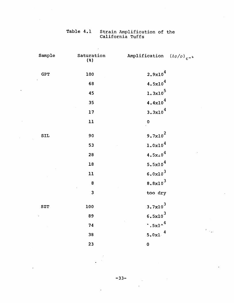
Table 4.1
Sample
Strain Amplification of theCalifornia Tuffs
GPT
-33-
Saturation(%)
100
68
45
35
17
11
90
53
28
18
11
8
3
100
89
74
38
23
Amplification (Ap/p) E
2.9x10⁴
4.5x10 4
1.3x10⁵
4.4x10⁴
3.3x10 4
0
9.7x10²
1.0x10 4
4.5x.04
5.5x10⁴
6.0x10³
8.8x10 3
too dry
3.7x10 3
6.5x10 3
".5x1^4
5.Oxl 4
0
SIL
SZT

Sample
RTTa
-34-
Saturation
100
83
66
47
35
82
68
53
100
75
31
11
7
93
72
19
14
4
Amplification (Ap/p) _
1.7x10⁵
4.2x10⁴
1.4x10⁵
2.3x10⁵
3.4x10 4
5. 0x10 4
1. 1x10⁵
2.4x10 4
2.1x10³
1.5x10 4
8.0x10⁴
6.4x10 4
5.5x10 4
2.6x10²
31.lxlO
1.3x10⁴
35.9x10
4.6x1J3
RTTb
DPRa
SHR

Table 4.2 Physical Properties of theCalifornia Tuffs
Sample Porosity(%)
GPT
RTT
DPR
SIL
SHR
SZT
10.7
3.7
17.9
35.6
37.2
17.1
Modulus(GPa)
10.0
12.5
3.5
2.4
2.2
3.3
Peak Sat.(%)
45
58 (av)
31
18
14 (av)
38
Max. Amplification
1. 3x10 5
2.3x10⁵
8.0x10 4
5.5x10 4
1.3x10⁴
5.0x1.04
-35-

CHAPTER V
Discussion
The electrical behavior of the rocks described above
was similar to typical wet rocks studied elsewhere (Brace,
Orange and Madden, [1965], Brace and Orange, [1968]), at
least in certain respects. Conduction appears to be largely
through water-filled pore space; surface conduction may be
important, particularly for samples containing clays, but
mineral conduction is probably not significant. An increase
in stress lowers resistivity for partial saturation, as was
the case for a granite (Brace and Orange, [1968]). However,
there are at least two characteristics of the tuffs which
are quite unusual, and require some discussion. First is
the high amplification factor, and the second is electrical
recoverability.
Amplification Factor
Madden has shown [1978] that amplification factor
ranges from about 1600 (granodiorite of 0.4 percent porosity
at 7.5 MPa) through 800 (granite of 0.9 percent porosity) to
about 100 for porous sandstones. Amplification factor here
was 103 to 10s (Figure 4.5) and 10' in Yamazaki's study.
-36-

Saturation and porosity seemed to be determining
factors for electrical amplification of strains. Both high
and low saturation tended to reduce amplification. At high
saturation there is only a small percentage increase in the
number of conduction paths before all the fluids have been
mobilized. Amplification factors under these conditions
would be low. As saturation decreases, a larger fraction of
the water is initially in the form of isolated pockets that
are subsequently joined. This situation leads to highest
amplification. For still lower saturations, an increasing
fraction of the water pockets do not join as stress is
applied. The percentage of newly interconnected cracks is
again low, and amplification is lower.
The stiffer rocks are not able to close cracks as well
as the lower modulus samples for a given stress. It might
be concluded that amplification would be low in this case.
However, there are two factors that counter this argument.
First, the higher water content in the stiffer rocks (at
peak saturation) overcomes the fact that crack closure is
not as effective. Second, the lesser pore volume tends to
make small changes in interconnectivity more pronounced.
This is particularly true for rocks with a greater fraction
of cracks than pores. Less stiff rocks do not require as
much water for maximum sensitivity because the crack closure
-37-

due to the larger strain is great enough to effectively
distribute the water.
Yamazaki [1966] found that for rocks of about the same
porosity, high amplification was associated with high
permeability. Based on other studies, Brace, [1977], high
permeability implies large pore diameter. Unfortunately, it
was difficult to determine a meaningful pore diameter in all
cases for these tuffs based on the SEM studies, so that his
observation could not be fully tested here. The tentative
conclusion was that amplification did not correlate with
.pore size. Clearly there is need here for further
petrographic work.
Recoverability
In many ways the most puzzling behavior of the tuffs is
the electrical recoverability during a stress cycle. No
other partially saturated rocks show this effect to any
degree. Two parameters seemed important: porosity and pore
size. Porosity is the dominant factor; the most porous
tuffs (35 percent) did not recover well. Recoverability
improved as porosity decreased or equivalently, as modulus
increased.
-38-

The more recoverable tuffs contained larger cracks and
pores, and coarser mineral structures. In samples with pore
diameters 100 times smaller (SIL), electrical resistance
increased insignificantly upon unloading. Perhaps the fine
gas bubble voids increased the capillarity within the
-sample, making it more difficult for water to retract as
stress is decreased. Sandstones also showed consistantly
poor electrical recoverability, probably a result of the
difference in pore structures between the two rock types.
A third factor, and one which would be difficult to
assess, must be surface properties of the different phases
in the tuffs. Perhaps recoverability requires a nonwetting
phase, such that water is dispelled from pores after stress
is released. Unfortunately it was not possible to determine
all the phases in the rocks, let alone their surface
characteristics. This too is a fertile area for future
studies.
-39-

CHAPTER VI
Conclusions
1) The rate of change of resistance with applied stress has
been shown to be very large, particularly for small strains,
in agreement with Yamazaki's results on certain tuffs from
Japan.
2) Amplification factors as defined at a strain of
10 range between 103 and 105 for the California tuffs.
3) Porosity and saturation are the key factors for optimum
amplification.
.4) Tuffs exhibit an electrical recoverability not observed
in other rock types.
5) Electrically sensitive tuffs exist near active faults
where they could be used as stress monitors for earthquake
prediction.
6) A preliminary investigation of electrical properties
similar to the chunk test would seem appropriate for
locating a field site, as a precise description of lithology
for a suitable rock is not available at this time.
7) Further studies on mineralogy, pore structure and
permeability would greatly improve the understanding of the
processes involved.
-40-

APPENDIX A
Studies of Nevada and Montana Tuffs
The initial phase of this project was aimed at
verifying the observations of Yamazaki and hopefully gaining
some insight into the processes involved. Yamazaki
demonstrated that the particular conditions of interest were
low stress and low saturation. Therefore the approach
chosen was to consider stresses only up to 6 MPa and
saturation levels generally less than 25 percent.
Three samples from the Nevada Test Site and two from
Montana were used in this first study (Table Al). .The
sample preparation and experimental procedure was exactly
the same as discussed previously for the California tuffs.
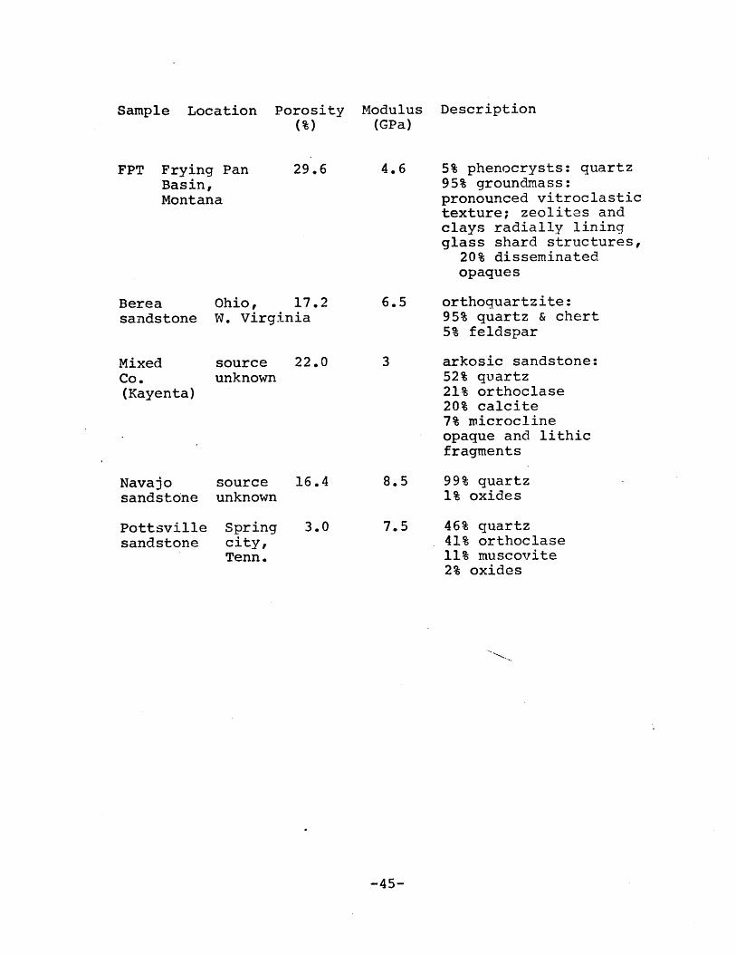
After testing these rocks, four sandstones were analyzed for
a comparison of rock types (Table Al).
-41-

Observations
Stress-strain curves for the tuffs and the Pottsville
and Berea sandstone are shown in Figure Al. Porosities are
indicated next to the curves. These tuffs are more linearly
elastic than many of the California rocks: there is little
if any hysteresis in the curves. Sandstones usually retain
a permanent strain after the stress cycle.
The effect of stress cycling on the electrical
properties is apparent in Figure A2. Tunnel Beds tuff
recoverd nearly completely upon successive loading, Berea
sandstone did not. The second cycle of Berea showed almost
no change in resistance. This behavior was typical of the
other sandstones, as seen in Figure A3. Although the degree
of recoverability varied among the tuffs, it was
consistently poor in the sandstones.
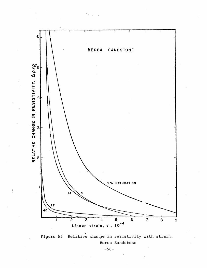
If only the loading curves are considered, both the
sandstones and the tuffs (with the exception of the
Pottsville sandstone), have high amplification factors at
low strains (Figures A4 and A5). Thus Yamazaki's unusual
observations have been verified. The amplification factors
as previously defined are compiled in Tables A2 and A3.
-42-

Discussion
Clearly rock type is an important parameter in the
electrical characteristics of these samples. After the
unrecoverable nature of the sandstones was observed, further
studies were concentrated solely on tuffs.
There were no identifiable trends of amplification
factor with porosity or saturation because the concept of
"optimum saturation" discussed earlier had not yet been
realized. The restricted range of low saturations led to
some misleading initial conclusions. Low saturation was by
forture ideal for Yamazaki's very porous rocks, but it is
not a key factor when considering tuffs in general.
After the work on California rocks revealed the
importance of saturation level, certain of the Montana and
Nevada tuffs were re-tested at the saturations predicted
from Figure 4.7. With little surprise, these rocks were
consistent with the California samples and fell nicely on to
the linear plot of Figure 4.7.
-4-3-

Table Al Rock Descriptions
Sample Location Porosity(%)
Modulus(GPa)
Description
TBT Nevada Test 17.6Site, TunnelBeds area 20
ATT Ammonia Tanks 5.8tuff, NevadaTest Site,Silent CanyonCaldera
RMT Ranier Mesa 14.2tuff, SleepingButte Calderasegment, NevadaTest Site
BLT Butte, 10.2Montana
4.1
8.5
8.5
11.0
Zeolitized ashfall tuff20% phenocrysts:
5% quartz15% plag & sanidine
5% lithic fragments75% groundmass:
40% clinoptilolite10% clay minerals15% opal & silica
minerals10% glass
40% phenocrysts:15% quartz15% plag & sanidine3% Ti rich augite5% opaques2% biotite
5% lithic fragments.55% groundmass: finegrained zeolitized ash& glass
phenocrysts:10% quartz10% plagioclaseX% opaquesX% Ti stained biotite
10% pumice fragments70% fine grainedgroundmass:
10% zeolites10% clay50% ash
phenocr-sts:10% q 'artz10% p agioclase5% bi tite
75% groundmass:20% plag lathesX % chlorite35% recrystallized
glass20% pumice fragments
-44-
Sample Location Porosity(%)
Modulus(GPa)
Description
FPT Frying PanBasin,Montana
29.6 4.6 5% phenocrysts: quartz95% groundmass:pronounced vitroclastictexture; zeolites andclays radially liningglass shard structures,
20% disseminatedopaques
Bereasandstone
MixedCo.(Kayenta)
Ohio, 17.2W. Virginia
sourceunknown
22.0
6.5
3
orthoquartzite:95% quartz & chert5% feldspar
arkosic sandstone:52% quartz21% orthoclase20% calcite7% microclineopaque and lithicfragments
Navajosandstone
Pottsvillesandstone
sourceunknown
Springcity,Tenn.
16.4
3.0
8.5
7.5
99% quartz1% oxides
46% quartz41% orthoclase11% muscovite2% oxides
-45-

SANDSTONES
TB
76
AT BL
.8 110.2 17.2
10-
LINEAR
Figure Al
STRAIN
Stress-strain curves of Nevada/Montana tuffs
and the Pottsville and Berea sandstones
RM
14.2
FP
U)towHrU)
2
0
T UF F S

1BEREA SANDSTONE
4.7% Saturation
-0
0 1 2 3 4 5
STRESS, MpaChange in resistance with stress, TBT,
108
10
E0
z
Cnw
610
Berea ss.Figure A2

I 2 3 4 5 6STRESS MPa
-Figure A3 Change in resistance with stress:
-48-sandstones
108
E 6=100
z
4I-
104

BUTTE LAPILLI TUFF2
0
H
z
-
wjzcc
2 3 4 5 6 7 8
strain , C,
Figure A4 Relative change in resistivity with strain, BLT-49-
% SATURATION
0 I
Linear
cc
(e)4
w
0z
9% SATURATION
13
402740
I 2 3 4 5 6 7 8Linear strain, E , 10
Figure A5 Relative change in resistivity with strain,
Berea Sandstone
-50-

Strain Amplification of theMontana/Nevada Tuffs
Sample
BLT
RMT
TBT
Saturation(%)
4.2
5.0
5.2
11.2
12.6
29.6
49.1
2.5
4.7
5.1
5.4
38.0
45.0
2.8
4.8
7.3
9.9
12.9
20.1
46.8
-51-
Table A2
Amplification (AP/P) -4
2.3xl04
2.5x10³
1.6x10⁴
8.1x10³
2.1x10⁴
3.0x10³
2.8x10⁴
5. 0x102
0
5. 0x102
6.6x10²
1.0x10⁴
1.6x10⁴
7.0x10³
38.0x10
8.0x10³
1.0x10⁴
1.0x10⁴
4.4x10³
32.0x10

Sample Saturation Amplification (Ap/p)(%)
FPT 2.1 2.2x10³
3.8 1.2x10³
6.7 1.7x10³
15.2 3.2x10⁴
17.1 2.4xl03
22.2 8.8x10 4
58.0 8.0x10²
ATT 7.0 1.2x10²
11.1 1.3x10²
14.3 1.5x10 3
18.6 5.0x10²
56.0 1.0x10 4
-52-

Strain Amplification of Sandstones
Saturation(%)-
Mixed Company(Kayenta)
3.8
7.6
21.8
34.3
44.0
94.0
2.5
5.6
12.3
19.3
33.0
4.7
9.2
13.1
26.9
40.0
Amplification (Ap/p)
9.2x10²
4.0x10 2
1.0x10⁴
1.6xl03
. 3.1x10 3
2.4x10⁴
3. 2x10⁴
9 .2-:103
8.6x10 2
4.4x10 4
3.9x10 4
1. 2x10⁴
1. 6x10 3
9.1x10²
-53-
Sample
Navajo
Berea
Table A3

Sample Saturation Amplification (Ap/p) -4(%)
Pottsville 6.4 0
8.5 0
13.9 0
21.0 0
24.9 0
32.5 0
42.5 1.3x100
63.4 1.0x10 1
-54-

APPENDIX B
The Chunk Test
This test was devised to quickly investigate the
electrical properties of samples while still in a crude hand
specimen configuration. Results were strictly qualitative,
as the geometry factors of the irregular shapes were not
precisely known. However, chunk tests performed on the
Nevada and Montana tuffs showed that resistance cycled in
the same manner as the cylindrical samples described in
Appendix A, although to a lesser degree due to the larger
sample size. Therefore, the chunk test was indeed valid for
a preliminary sorting by electrical properties. Table Bl
lists the samples used in this test along with their
locations, and a brief hand specimen description.
Sample Configuration
Rock fragments were broken off into more or less equal
shapes about 5 cm long. Two lead sheets, 0.02 cm thick by
1.9 cm square were conformed on to opposite sides of the
sample, with copper wire soldered to each sheet, leading to
the resistance measuring circuit. The lead was epoxied
around the edges to the rock to avoid separation. The whole
assemblage was then. potted in Dow Corning Sylgard 186
-55-

silicone elastomer with the wires extending out of the
cylindrical case of rubber (Figure Bl).
Experimental Procedure
Potted samples were placed in a beaker of kerosene or
water inside a 15 cm diameter argon gas pressure vessel.
Kerosene is prefered to prevent corrosion of the vessel.
However, Sylgard swells in kerosene and the samples must
then be coated with Kenyon K-Kote to avoid expansion, a
process which adds a few days to the sample preparation.
Aesistances were measured at natural water content by
method 2 of Appendix D, while increasing and decreasing
hydrostatic pressure to a maximum of 5 MPa. The set-up is
schematically illustrated in Figure B2.
Data
Figures B3 through B5 show the electrical resistance
response to stress cycling on a number of the California
tuffs. Samples which exhibited little or no change are not
included. The unloading curves consistently fell below the
loading curves as with the cored rocks.
-56-.
Samples are ordered in terms of relative resistance
change in Table B2. Those with an asterisk were the ones
chosen for more detailed study. Some very sensitive rocks
were not selected because of their friability.
-57-

Table Bl
Sample Locati
PIN Pinnacles NMonument
SJB San Juan Gr(Salinas RdSan Juan Ba
COT Stony PointQuarry, Cot
CMV CoomsvilleNapa
MWT MontecelloNapa
SIL Silverado iSt. Helena
PET Petrified FRd., Calist
SIHR St. HelenaSt. Helena
DPR Deer Park RSunset Poir
Location and Hand Specimen Descriptionsof the California Tuffs
on Hand Specimen Description
ational Dense green tuff, numerous lithicfragments and phenocrysts
ade Rd. Conglomerate in tuffaceous matrix,.), pebbles up to 0.75 cm in diameterutista
Fine grained powdery grey clay inati 0.5 cm thick bed
Rd., Plum colored matrix, lithicfragments up to 1 cm, plagioclaselathes visible
Rd., Welded grey pumice fragments,light and porous
rail, White rhyolitic tuff, fragments ofwhite pumice up to 1 cm, lithicfragments (0.5 cm), plagioclaselathes
orest Rhyolitic tuff similar tooga Silverado, more weathered & friable
Rd., Coarse, grey, hard nd verycrystalline tuff, e: tensive andwell exposed in roa" cuts
d., .Very dense fine grained purple andt grey matrix with large pores; no
noticeable lithic fragments
-58-

Hand Specimen Description
RLS Robert LouisStevenson StatePark, Calistoga
GPT Little GrizzlyPeak,Berkeley Hills
RTT Round Top Hill,Berkeley Hills
SZT Siesta cinder coneSiesta Valley
DRY Grizzly Peak Rd.,Berkeley Hills
Very hard grey tuff weathers toyellow-brown; lithic fragments upto 0.5 cm; fractured
Large massive outcrop, coarse anddense lithic fragments up to 2 cm,highly fractured
Basalt tuff; black, fractured andweathered into boulders; part of acinder cone 400 m in diameter
Brown lithic tuff filled withveins of zeolite
Buff colored airfall tuff,weathered and friable laver a fewmeters thick
-59-
Sample Location

copper wire
lead sheet
sample
rubber
Figure Bl Sample configuration for the chunk test
F.igure B2 Chunk test experimental apparatus
-60-

I 2 3 4 5
STRESS MPo
Figure B3 Change in resistance with stress;
SHR, DPR, RLS, DRY.
-61-
0
E
(nC0
w'

106
tnE.c:0
w
. 10
O-
I 2 3 4 5 6
STRESS MPo
Figure B4 Change in resistance with stress;
MWT, SZT, GPT.
-62-

1 2 3 4 5 6
STRESS MPa
Figure B5 Change in resistance with st--ess;
SJB, SIL, RTT, COT.
-63-
10
(n
E0
wz(n(nw

Table B2
Good
COT
DRY
GPT*
RTT*
Relative Ordering of Electrical Propertiesof California Tuffs
Fair
SZT*
RLS
DPR*
SIL*
Poor
SHR*
SJB
MWT
No Effect
CMV
PET
PIN
* Studied in detail
-64-
APPENDIX C
Stress-Strain and Electrical Behavior of
Selected California Tuffs
This section contains the complete set of data on the
California tuffs that were not included in chapter 4, as
they are similar to the examples shown there. Stress-strain
curves for the six tuffs are illustrated in Figure Cl.
Figures C2 and C3 show the change in resistance with stress
for each sample at an arbitrary saturation. The curves were
chosen to show the most typical electrical recoverability of
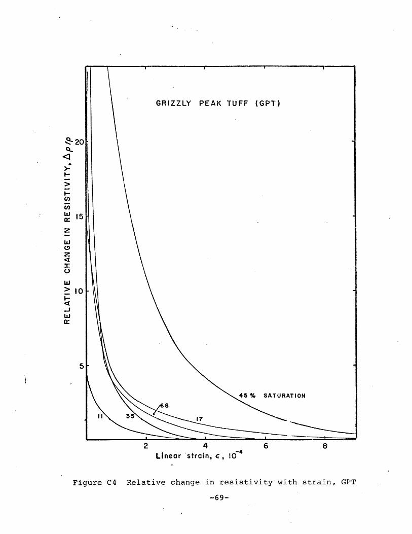
that sample. Figures C4 through C8 are plots of the
relative change in resistivity with strain and were derived
from the stress-strain and resistance data.
-65-

RTT GPT DPR SIL
LINEAR STRAIN
Figure Cl Stress-strain relation for the California tuffs
SHR0.
(n)
(14
U)4
2
0
SZT
10-3

GPT 35% Saturation
SIL 18 % Saturation
SHR 10 % Saturation
I 2 3 4 5 6STRESS MPa
Figure C2 Change in resistance with stress;
GPT, SIL, SHR.-67-
108
07
106
05

106 DPR 10% Saturatiorz
SZT 74 % Saturatio
105
RTT 90% Saturati
1041 2 3 4 5 6
STRESS MPa
Figure C3 Change in resistance with stress;
DPR, SZT, RTT
$20
Q-
15C:
10
5
45 % SATURATIONz8
35 35
2 4 6 8Linear strain, c , >0
Figure C4 Relative change in resistivity with strain, GPT
-69-

ST. HELENA ROAD (SHR)
4
-
zWz
26 % SATURATION
10
73
0 10 20 30Linear strain, E , 10
Figure C5 Relative change in resistivity with strain, SHR
-70-

12
10
mCC
z 6
(Dz
-
-
2- 38% SATURATION
010 20 30Linear strain, C 4
Figure C6 Relative change in resistivity with strain, SZT
-71-

12
DEER PARK ROAD (DPR)
10
8
(D)
z6
-Jw 4
31 7% SATURATION
2 75
95
0 2 4 6 8 10 12 14 16 18Linear strain, E 104
Figure C7 Relative change in resistivity with strain, DPR
-72-

50
40
m30
z
zr20
m
66
10
100% SATURATION
47
583I0'
I 2 3 4 5 6 7 8 9
Linear strain, e, 10
Figure C8 Relative change in resistivity with strain, RTT
-73-

APPENDIX Dl
Resistance Measuring Techniques
There are several techniques for measuring the
resistance of a rock, each with trade-offs on ease and
accuracy. Most of these methods involve matching the
voltage across a variable resistance decade with that across
the rock sample. In all cases, the source voltage was kept
at 10 Hz AC, to minimize any frequency effects that could
occur at higher frequencies. See Appendix D2 for a nore
complete description of frequency effects.
Method- 1.
Rrock
V. ti/ M Vin B
Rbox M VA
The particular circuit used for the early work on the
Nevada and Montana tuffs was the same as that in Brace,
Orange and Madden, [1965]. VA and VB are measured on a
vacuum tube volt meter (HP model 40011). From the above
circuit diagram, it follows that V =VB and the system is a
voltage divider where
VA RoxV. R + Rin rock box

Since Rb is known and a particular VA/V. is chosen,
then Rrock can be calculated. To simplify the calculation,
assume that Rbox is much less than Rrock , by appropriately
adjusting the voltage ratio.
V.Now Rrock = Rbox VA
The ratio VA /Vin is determined to make the resistance fall
in a reasonable range on the decade box and to introduce no
significant errors. For example, with Vin /VA lo0
Rrock = 100R box (Turn the voltmeter range down by two
orders of magnitude to measure VA , then adjust the decade
until the meter needle comes to the same point as it did for
VB)-
A 1% theoretical error is introduced because
Rexact rock =99Rbox * The difference is considered
negligable. By turning the voltage down in this manner, it
is possible to measure rock resistances that are greater
than the resolution of the variable resistance decade.
The advantage of this technique is that it is quick and
requires no calculation. In order to find t'e resistance of
the rock, one need only add two orders of mi nitude on to
the resistance read off the decade box. Most of the Nevada
and Montana tuff samples were measured in this way.
-75-

Problems: Since the signal to be measured on the meter
has been reduced substantially, there is a potential problem
of noise dominant errors. In fact if V /Vin = 1000, the
signal to noise ratio is high enough that the measured
resistance of the rock will have a noticeably large error
(as much as a factor of 10). In the noise dominant
situation, if V /V. is chosen to be 1/10 instead of 1/100A in
or 1/1000, then the signals are larger and the resistance
box gives better resolution. The exact formula for
Rrock must be used, otherwise there is a 10% error:
Rrock 9Rbox'
On the practical side, this choice of VA/Vin is not as
quick, as it requires more mental gymnastics to calculate 9R
than 10R. However, it is more accurate.
If the resistance of the decade, which has a maximum of
1 megohm, approaches the input impedance of the meter, then
the effective resistance is reduced:
1 =1 + 1
Reffective Rbox meter
R = Rbox . Rmetereffective Rbox + Rmeter
The effective value is substituted into the R values:
VA Rbox VA Reffective7 R + R becomes - R + Rin rock box in rock effective

The HP 400H voltmeter has an input impedance of roughly
2.5 megohms. This impedance is rather low and should be
taken into account when dealing with dry rocks whose
resistance can be as high as 10 megohms.
Method 2.
+ +
in M- box R rock _
R F
Method 2. involves the same technique of matching
voltages as method 1. A voltage is chosen with the switch
on R rock Then with the switch on Rbox, the resistance is
adjusted until the same voltage is obtained as through the
rock. Now Rrock=Rbox* An additional resistor RF is
necessary in this circuit otherwise Vmeter always equals
Vin*
Choice of RF: To find a suitable value of RF , the
sensitivity of the meter is analyzed with respect to the
power transfer between the circuit and the load (rock). By
Joule's Law, 22 ____R V Rr
pR +Rr r (1 + RF / Rr 2
-77-
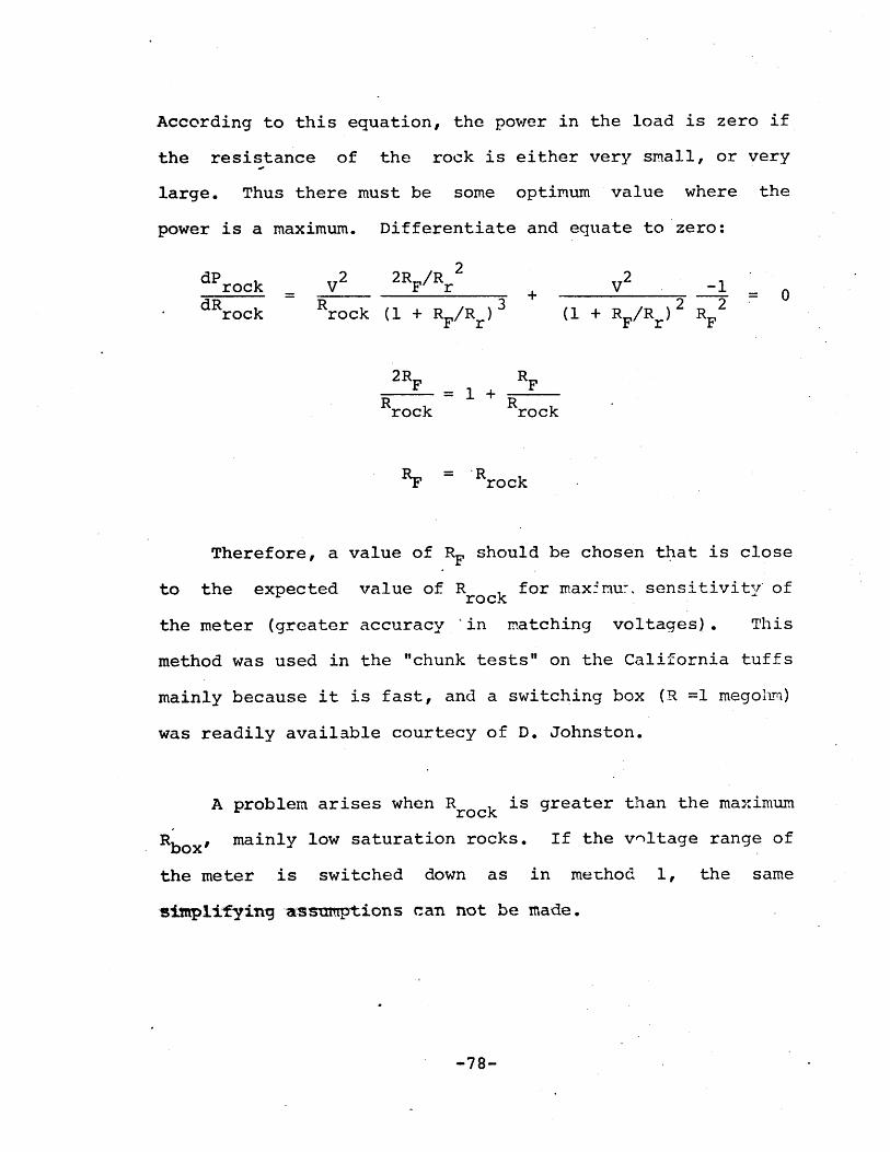
According to this equation, the power in the load is zero if
the resistance of the rock is either very small, or very
large. Thus there must be some optimum value where the
power is a maximum. Differentiate and equate to zero:
dP 2 2R /R 2rock _ V F r + V - 0dR R ~ l+RR 3 (lRR 2 R2
- rock rock (1 + RF/Rr) (1 + RF/Rr) RF
2R RF = 1+ F
R R -rock rock
RF = rock
Therefore, a value of RF should be chosen that is close
to the expected value of R for maximu. sensitivity~ ofrock
the meter (greater accuracy 'in matching voltages). This
method was used in the "chunk tests" on the California tuffs
mainly because it is fast, and a switching box (R =1 megohm)
was readily available courtecy of D. Johnston.
A problem arises when Rrock is greater than the maximum
Rbox, mainly low saturation rocks. If the vnltage range of
the meter is switched down as in method 1, the same
simpiifying assumptions can not be made.
-78-

RkV. ( rock
in Rrock + RF Ml
Rb MV ( boxin Rbox + R F t M2
if V Ml = 0VM2' then
R rockRrock +KRF
= 100Rbox
Rbox + RF
RrockRbox + RrockRF = 100RboxRrock + 100 RboxRF
Rrock (RF - 99Rbox
R1OR -9 RR100boxRF-rock RF -99Rbox
Since RF = 106 ohms,
then
100 RboxR F
This is true if Rmeter is much greater than Rrock'
Otherwise the same problem with a low impedance meter exists
because the meter is in parallel with the rock and the box.
-79-

box effective ox
'rock effective Rrock equation in box
As can be seen from the above discussion, the switching
box method is no longer quick when trying to measaure high
impedance rocks.
Method 3.
V.in VB
Bridge method: RA and RB are fixed resistors.
adjusted until the bridge is balanced, i.e. the meter reads
zero volts. Then VA=VB'
VA RAV. R + Rin A box
RB
R + RB rock
VB
V.in
RA (RB + R ) = R(R + RR( +Rrock B A box
rock R A box
-80-
1
meter
Ret1mete
Rbox is

Note that the response does not in any way depend on
the meter. The ratio of RB to RA is chosen co scale Rbox to
Rrocke For instance, if Rrock max = 1 megohm and
Rbx max = 1 megohm, then make RB/RA =10. Now resistance
measurements greater than Rbox can be made. The absolute
magnitudes of RB and RA are set to gain the maximum meter
sensitivity to the null. RB is chosen to be around the same
order of magnitude as R rock. (See sensitivity derivation in
method 2). Then RA~ 100 kilohm for a typical low saturation
rock. This value is optimum for the decade box, since it
has maximum resolution in the middle ranges.
Because the resistance of the rock can vary widely
depending on the mineralogy and degree of saturation, say
between 1 kilohm and 10 megohm, it may be best to have two
sets of resistors for optimum sensitivity. Each set has
appropriate values of RA . This modification is not
tremendously important to the workings of the circUit unless
there is reason to be concerned with sensitivity.
RB = 10 kilohm for 1 kilohin<R rock<100 kilohm
and RB = 1 megohm for 100 kilohm<R rock<1 megohm
The bridge method has a definite advantage over the
other two methods. Since the meter does not enter into any
calculations, there are no errors due to low input impedance
or noise.
-81-

A problem common to all techniques: The source for the
resistance measuring circuit has an alternating current of
10 Hz. The strain gauge and corresponding circuit on the
other hand runs on DC, and is designed to detect small
changes in the DC voltage. Since the AC and DC currents are
juxtaposed in the sample, there is a coupling in which the
AC current appears in the strain signal. The epoxy between
the rock and strain gauge is not always enough to ensure
proper insulation, particularly with saturated samples. The
result is a 10 Hz vibration of the pen along the strain axis
as much as 2 cm wide, (leading to a mighty fuzzy
stress-strain curve!).
There are two solutions:
1) Disengage the pen while making a resistance measurement.
This tends to slow down the experiment, since there are
thirteen measurements to be made on each run, therefore
twenty-six times to flick the pen. The chance for human
error arises since one sometines forgets to engage the pen
after a measurement, and part of the stress-strain curve is
lost.
2) Build a low pass filter into the chart input. A somewhat
detailed description of the filter is in order as it has a
significant effect on the chart response.
-82-
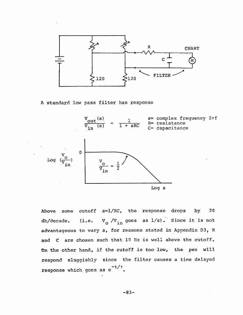
FILTER
A standard low pass filter has response
V (s)
VCiu (s) 1 + sRCin
s= complex frequency 2TrfR= resistanceC= capacitance
Log ( ) v -0 2inin
Log s
Above some cutoff s=l/RC, the response drops by 20
db/decade. (i.e. V0 /Vin goes as l/s) . Since it is not
advantageous to vary s, for reasons stated in Appendix D3, R
and C are chosen such that 10 Hz is well above the cutoff,
On the other hand, if the cutoff is too low, the pen will
respond sluggishly since the filter causes a time delayed
response which goes as e-t/T
-83-
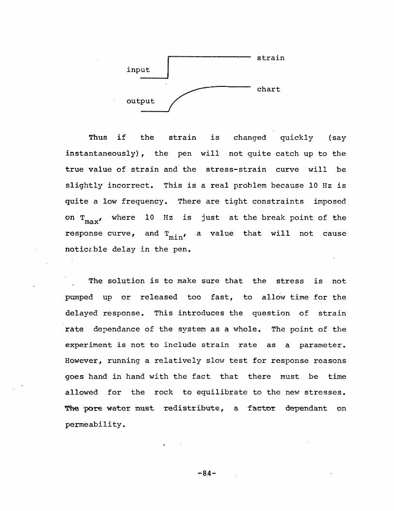
input
chart
output
Thus if the strain is changed quickly (say
instantaneously), the pen will not quite catch up to the
true value of strain and the stress-strain curve will be
slightly incorrect. This is a real problem because 10 Hz is
quite a low frequency. There are tight constraints imposed
on Tmax, where 10 Hz is just at the break point of the
response curve, and T min , a value that will not cause
noticEble delay in the pen.
The solution is to make sure that the stress is not
pumped up or released too fast, to allow time for the
delayed response. This introduces the question of strain
rate dependance of the system as a whole. The point of the
experiment is not to include strain rate as a parameter.
However, running a relatively slow test for response reasons
goes hand in hand with the fact that there must be time
allowed for the rock to equilibrate to the new stresses.
The pore water must redistribute, a factor dependant on
permeability.
-8.4-

Note that if the experiment were run at a higher
frequency, then "sluggishness" could be avoided altogether.
When the amplitude of the noise is low, a smaller capacitor
can be used to alleviate the response problem. At even
higher frequencies, say 10 k1z, the pen will not even have
time to respond to the noise.
Both solutions to the noise problem have their
disadvantages. One might wonder why the resistance is not
measured with DC. This would require the actual movement of
ions through the sample. If it is assumed that the charge
is being transmitted primarily by the water phase rather
than by mineral conduction, then a DC current would tend to
electrolyze the water. At one of the electrodes there would
be dissociated water forming oxygen and hydrogen gas. This
is far from a desirable situation, especially since fixed
partial saturation is an important factor in the experiment.
-85-
APPENDIX D2
Choice of Electrode Material
The ideal electrode material for measurina resistance
should have the following qualities:
1) Be a good conductor.
2) Maintain a good electrical contact with the sample
3) Have no stress effect (change in measured resistance with
applied stress) .
4) Have no frequency effect, or at least no frequency effect
within a given working range.
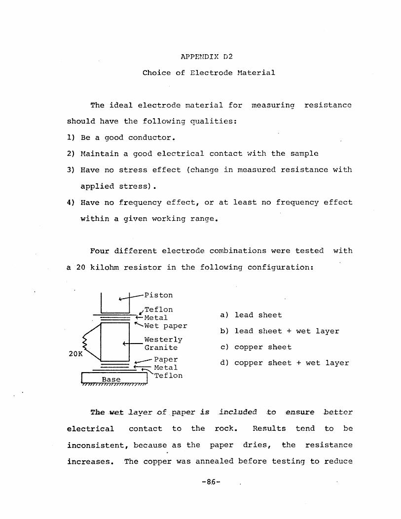
Four different electrode combinations were tested with
a 20 kilohm resistor in the following configuration:
Piston
+-Teflon a) lead sheet_ 4Metal
'r'-Wet paper b) lead sheet + wet layerWesterlyGranite c) copper sheet
20K20K__ -Paper d) copper sheet + wet layer
+-Metal
Base Teflon
The wet layer of paper is included to -ensure better
electrical contact to the rock. Results tend to be
inconsistent, because as the paper dries, the resistance
increases. The copper was annealed before testing to reduce
-8.6-

strain hardening effects, and enable the sheet to conform
better to the rock surfaces. However, as the copper is
stress cycled many times, strain hardening can become
permanent, even after annealing. The electrical conduction
properties of the copper lattice will vary slightly because
of distorted grains and dislocation pile-ups. This effect
will also cause the material to become less pliable.
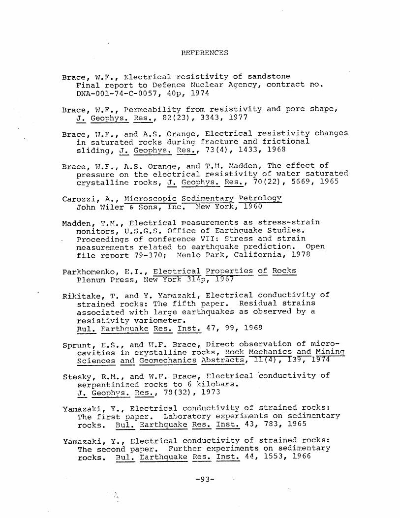
There appeared to be no significant frequency
dependance with the various electrode combinations, however
both the wet and dry copper in the stress test showed higher
resistance values than the correct value of 20 kilohms + 200
ohms (Figure Dl).
The dry lead sheet was chosen as the electrode
material. Lead is able to conform better to the surface of
the sample than the copper sheet, due to its low yield
stress. This is particularly important when testing
sandstones, which can have a very course surface. There was
no apparent stress effect with the dry lead.
-87-

T COPPER
.066I
9"
9'9'9'9'9'
9'.4
9'
9' j
I
"IAI 9'
/ '9',
It
DRY LEAD
40 50
S T R E S S , MPa
Figure Dl Stress effect of various electrodes, 20K resistor
'
WE
2.10
z
I-cc
DRY COPPER/
2.00
I0000I
at 10 HZ
APPENDIX D3
Freguency Effects
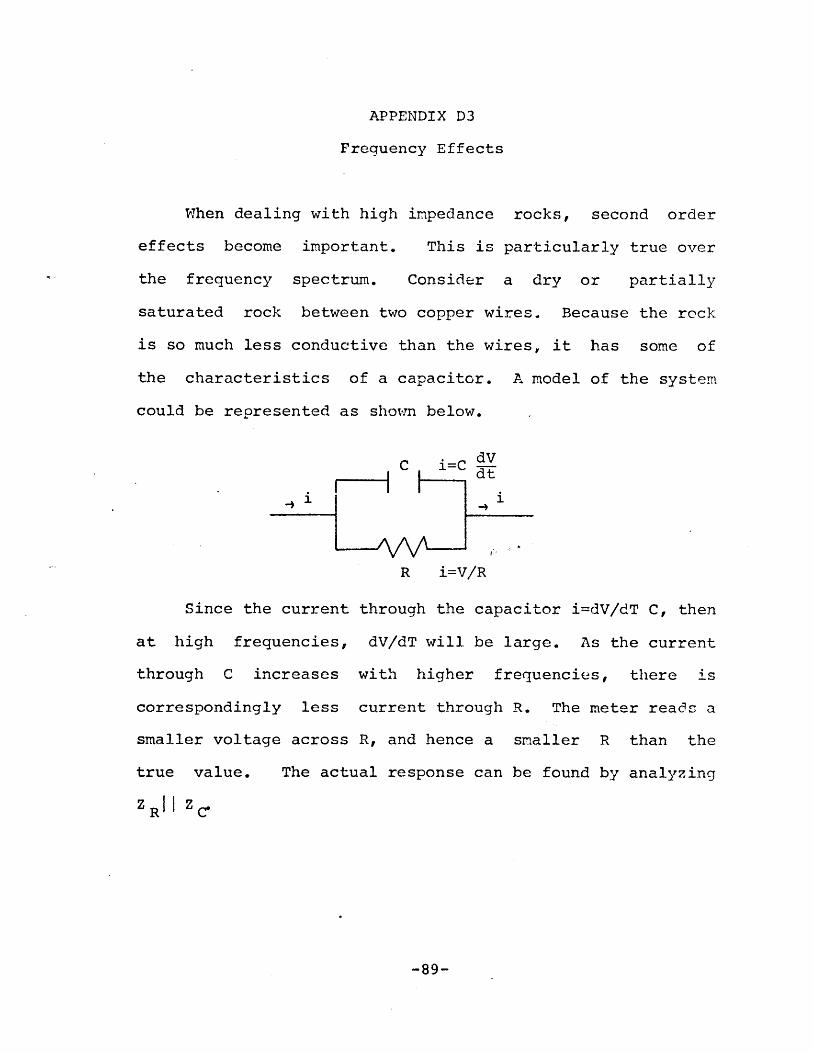
When dealing with high impedance rocks, second order
effects become important. This is particularly true over
the frequency spectrum. Consider a dry or partially
saturated rock between two copper wires. Because the rock
is so much less conductive than the wires, it has some of
the characteristics of a capacitor. A model of the system
could be represented as shown below.
.dVC i=C --
dt
R i=V/R
Since the current through the capacitor i=dV/dT C, then
at high frequencies, dV/dT will be large. As the current
through C increases with higher frequencies, there is
correspondingly less current through R. The meter reads a
smaller voltage across R, and hence a smaller R than the
true value. The actual response can be found by analyzing
ZR11 ZC
-89-

Z = R
ZC jfCR1 jf .1C jC
+ jfC = 1 jfR
Log Z
Z R1 + jfCR
Log f
When the frequency is small, Z=R, and when the frequency is
large Z falls off as 1/w. There will be a family of curves
for varying resistance.
The accuracy of standard film resistors at 107 ohms
breaks down at 100 Hz, therefore a frequency of 10-100 Hz is
suitable to eliminate the capacitance effects of the fixed
resistors in the electrical resistance bridcre of method 3.
The plot in Figure D2 was obtained using rocks of
varying saturation with no axial stress. The tuffs have a
high internal capacitance. Since the point of this
experiment is not to investigate the frequency dependance of
resistance in the tuffs, it is necessary to run the
frequency as low as possible to measure the high impedance
samples. Above 10 .ohms (at 10 Hz), the resistance values
are already on the sloping part of the response curve. Thus
they represent a minimrum resistance, and are a contributing
-90-

factor to the scatter in the data. Frecuencies of less than
10 Hz are not desirable due to the electrolyzing problems of
a DC-like current.
-91-

RTT (77)
GPT (45)
SZT (75)
E
0z
SZT (86% Sot.)
I:
10- sHR (58)
SIL (65)
S HR '(34)
lei00O', 102 103 04105
FREQUENCY (Hz)
Figure D2 Resistance fall-off with frequency for the
California tuffs at varying saturations
REFERENCES
Brace, W.F., Electrical resistivity of sandstoneFinal report to Defence Nuclear Agency, contract no.DNA-001-74-C-0057, 40p, 1974
Brace, W.F., Permeability from resistivity and pore shape,J. Geophys. Res., 82(23), 3343, 1977
Brace, W.F., and A.S. Orange, Electrical resistivity changesin saturated rocks during fracture and frictionalsliding, J. Geophys. Res., 73(4), 1433, 1968
Brace, W.F., A.S. Orange, and T.M. Madden, The effect ofpressure on the electrical resistivity of water saturatedcrystalline rocks, J. Geophys. Res., 70(22), 5669, 1965
Carozzi, A., Microscopic Sedimentary PetrologyJohn Wiler & Sons, Inc. New York, 1960
Madden, T.M., Electrical measurements as stress-strainmonitors, U.S.G.S. Office of Earthquake Studies.Proceedings of conference VII: Stress and strainmeasurements related to earthquake prediction. Openfile report 79-370; Menlo Park, California, 1978
Parkhomenko, E.I., Electrical Properties of RocksPlenum Press, New York 314p, 1967
Rik'itake, T. and Y. Yamazaki, Electrical conductivity ofstrained rocks: The fifth paper. Residual strainsassociated with large earthquakes as observed by aresistivity variometer.Bul. Earthrauake Res. Inst. 47, 99, 1969
Sprunt, E.S., and W.F. Brace, Direct observation of micro-cavities in crystalline rocks, Rock Mechanics and MiningSciences and Geomechanics Abstracts, 11(4), 371974
Stesky, R.M., and W.F. Brace, Electrical conductivity ofserpentinized rocks to 6 kilobars.J. Geophys. Res., 78(32), 1973
Yamazaki, Y., Electrical conductivity of strained rocks:The first paper. Laboratory experiments on sedimentaryrocks. Bul. Earthquake Res. Inst. 43, 783, 1965
Yamazaki, Y., Electrical conductivity of strained rocks:The second paper. Further experiments on sedimentaryrocks. Bul. Earthquake Res. Inst. 44, 1553, 1966
-93-