electrical properties and structure of … mamunya - lecture2.pdf · structure of polymer...

ELECTRICAL PROPERTIES AND ELECTRICAL PROPERTIES AND STRUCTURE OF POLYMER COMPOSITES STRUCTURE OF POLYMER COMPOSITES

WITH CONDUCTIVE FILLERSWITH CONDUCTIVE FILLERS2. Filled polymer blends: influence of 2. Filled polymer blends: influence of morphology on spatial distribution morphology on spatial distribution

of filler and electrical propertiesof filler and electrical properties

Ye. P. MamunyaInstitute of Macromolecular Chemistry

National Academy of Sciences of Ukraine Kiev, Ukraine

[email protected]

• Immiscible polymer blends create the two-phase systems with variety of morphologies, for example:a) dispersed structure (TPU/PP=80/20)

b) matrix-fiber structure (SAN/PA=70/30)

c) lamellar structure (PP/EPDM=80/20)

d) co-continuous structure (PS/PE=75/25)

• Type of structure mainly depends on the fraction ratio of components, processing (technological regimes) and viscosity ratio.

Types of the polymer blend structureTypes of the polymer blend structure

P. Potschke, D. R. Paul. J. Macromol. Sci., Part C-Polym. Revs., 2003, C43, 87-141.

2

D.A. Zumbrunnen. S. Inamdar. Chem. Eng. Sci., 2001, 56, 3893–3897.

• Schematic description of theblend morphology develop-ment along the axis of a twin-screw extruder for a polymerpair AB.

• Conditions: 1) φB > φA, ηA > ηB

2) φB < φA, ηA < ηB

Forming of the blend structure during processingForming of the blend structure during processing

3

P. Potschke, D. R. Paul. J. Macromol. Sci., Part C-Polym. Revs., 2003, C43, 87-141.

J.K.Lee, C.D.Han. Polymer, 2000, 41, 1799–1815.

J.K.Lee, C.D.Han. Polymer, 1999, 40, 6277–6296.

Structural model of development of the blend Structural model of development of the blend morphology depending on the componets ratio morphology depending on the componets ratio

4

• Depeding on fraction ratio A/B of components the morphology of polymer blend changes from the insulated inclusions of polymer B within polymer A (at low content of polymer B) to the co-continuous structure at equal content of the phases and further to the inclusions of polymer A within polymer B (at low content of polymer A).

A

B

A

B

B

A

B

A

B

A

A B

Polymer A / Polymer B = 100 / 0






Polymer blend based on:• Polymer A:cellulose acetate butyrate• Polymer B:polyoxymethylene

There are three regions of mechanical properties of this polymer blend that strongly depend on the structure: (1) corresponds to inclusions of B in A; (2) the polymer components behave as the connected phases; (3) corresponds to inclusions of A in B.

Morphology of polymer blend and derived Morphology of polymer blend and derived mechanical propertiesmechanical properties

Ye. P. Mamunya, E. V. Lebedev, E. N. Brukhnov, Yu. S. Lipatov.Vysokomolek. Soed., 1979, A21, 1008-1013 (in Russian).

5

ε, %σi, kg cm/cm2

σt, σy, kg/cm2

Content of polymer B

A

B

a

A

B

A/B

b

• Thickness of the interfacial layer δs is 2-10 nm and comparable with length of molecular segment.

• Thickness of the transition layer δt is up to 1 μm and defined by conditions of the structure forming.

Yu.S. Lipatov. Physical chemistry of filled polymers.Moscow: Chemistry, 1977 (in Russian).

a bδs δt

a b

δs δt

δs δt

a) TmA<Tproc<TmB

b) TmA<Tproc>TmB

Polymer blend PE-POM = A-B

Temperature of processing

Interfacial region in polymer blendsInterfacial region in polymer blends

Yu.S. Lipatov, Ye. P. Mamunya, E. V. Lebedev, N.A. Sytenko, G.Ya. Boyarskii. Vysokomolek. Soed., 1981, B23, 282-287 (in Russian).

6

Filling of polymers and polymer blendsFilling of polymers and polymer blends

Usually the polymers can be filled for several reasons:• To reduce the cost of polymer product. The cheap and widespread fillers are used;

• To improve the mechanical characteristics (toughness, bendingstrength etc.) of polymer. The reinforcing fillers are used.

• To obtain the colored polymer product. The pigments are used.

• To create the composite material. Content of filler in a polymer is very high (close to the limit of filling). The fiber fillers are often used.

• To impart new properties to the polymer. The functional fillers are used, for example conductive filler (carbon black, dispersed metals) that transforms filled polymer from insulating to conductive state.

• Filing of polymer blend with functional filler suggests additional potential in properties of the functional polymer systems because of heterogeneous structure of the polymer matrix that changes the spatial distribution of the filler. It is very important for conductive polymer systems.

7

• Heterogeneity of polymer blend can influence on spatial distribution of filler in the polymer matrix

• Immiscible polymer blend is two-phase system with developed interfacial region

• Generally 4 cases of spatial distribution of the filler can be realized in the polymer blend:

Influence of heterogeneity of polymer blend on the Influence of heterogeneity of polymer blend on the spatial distribution of filler spatial distribution of filler

8

Filler occupates both of polymer phases

Filler occupates one of twopolymer phases

Filler is localized on the interface

Filler occupates second oftwo polymer phases

filling

• Last three cases of filler distribution are of the highest interests because of nonuniform distribution of filler.

9

Generally 5 methods of filling of the polymer blend exist:

Electrical properties of composites depend on the conductive filler distribution and consequently on the method of filling

Influence of processing on the spatial Influence of processing on the spatial distribution of filler distribution of filler

Filler occupates both of polymer phases

Filler occupates one of twopolymer phases

Filler is localized on the interface

Filler occupates second oftwo polymer phases

filler → polymer 1polymer 2 FPB

polymer 1filler → polymer 2 FPB

filler → polymer 1filler → polymer 2 FPB

polymer 1+

polymer 2 FPBfiller +

polymer 1polymer 2 filler → FPB

1

2

3

4

5

Methods 1- 4 are two-stages, method 5 is one-stage.

polymer 1 polymer 2

processing

filler

filledpolymer blend

10

Variation of the composite composition leads to phase inversion in such a way:

Nonconductive matrix with inclusions of conductive phase

Co-continuous structures of conductive and non-conductive phases

Conductive matrix with inclusions of nonconductive phase

First, the composite is not conductive

Separated inclusions are merged creating the continuous filled phase which provides the appearance of jump of the conductivity

When conductive phase becomes a matrix, the con-ductivity increases slowly due to the decrease of the nonconductive inclusions

Structure

Conductivity

Correlation structureCorrelation structure--conductivity in filled conductivity in filled polymer blendspolymer blends

conductivenonconductive

Filler volume fraction, ϕ

Con

duct

ivity

, log

σ

ϕc

percolation threshold

Region 1

Region 2

Region 3

11

Structure and conductive properties of filled Structure and conductive properties of filled polymer blendpolymer blend

Conductivity of filled polymer blend is a function of the filler content and reflects its heterogenious structure.

Region 1 – the composite is non-conductive, the polymer blend consists of nonconductive polymer 1 with inclusions of filled conductive polymer 2 phase.

Region 2 – Co-continuous conductive and non-conductive unfilled polymer 1 – filled polymer 2 phases. It is a region of percolation, the conductivity sharply increases at ϕ > ϕc.Region 3 – Structure of composite consists of conductive matrix (filled polymer 2) with inclusions of nonconductive polymer 2 phase. The conductivity slowly increases.

J. Feng, C-M. Chan. Polym. Eng. Sci., 1998, 38, 1649-1657.

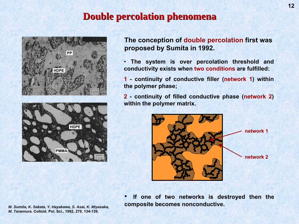
Double percolation phenomenaDouble percolation phenomena

The conception of double percolation first was proposed by Sumita in 1992.

M. Sumita, K. Sakata, Y. Hayakawa, S. Asai, K. Miyasaka, M. Tanemura. Colloid. Pol. Sci., 1992, 270, 134-139.

PP

HDPE

PMMA

HDPE

• The system is over percolation threshold and conductivity exists when two conditions are fulfilled:

1 - continuity of conductive filler (network 1) within the polymer phase;

2 - continuity of filled conductive phase (network 2) within the polymer matrix.

network 1

network 2

• If one of two networks is destroyed then the composite becomes nonconductive.

12

13

3 factors define the spatial distribution of filler in the two-componets polymer matrix:

Thermodynamic factor

Relationship between interfacial tensions polymer 1 – filler (γp1f), polymer 2 – filler (γp2f) and polymer 1 – polymer 2 (γpp)

Kinetic factor Relationship between viscosities of polymer 1 (ηp1) and polymer 2 (ηp2)

Processing factor

Methods of the filler introduction into the two-components polymer matrix

The main conditions to realize the irregular spatial The main conditions to realize the irregular spatial distribution of filler in polymer blenddistribution of filler in polymer blend

M. Sumita, K. Sakata, S. Asai, K. Miyasaka, H.Nakagawa.Polym. Bull., 1991, 25, 265-271

Parameters, mJ/m2Components of polymer blend γp γpf γpp

HDPE – CBPP – CBPMMA – CBHDPE – PPHDPE – PMMAPMMA - PP

25.920.228.1

---

13.1-12.217.1-16.712.2-14.6

---

---

1.28.66.8

γCB = 55 mJ/m2

BA

CBBCBA

−

−− −=

γγγω

Wetting coefficient

Influence of surface tension on the morphology of Influence of surface tension on the morphology of filled polymer blendfilled polymer blend

PP

PMMA

PP

HDPE

PMMA

HDPE

γA-CB, γB-CB – interfacial tensionpolymer-filler

γA-B – interfacial tension polymer-polymer

Conditions of filler ditribution

ω > 1 CB is distributed within B phase-1 < ω < 1 CB is distributed at the interface

ω < -1 CB is distributed within A phase

14

15

Behaviour of the filler particle on the boundary between components in polymer blend

c

0,0 0,1 0,2 0,3-16

-12

-8

-4

0

lg (σ

, См

/м)

ПП/ПЭ-сажаметод А

2 1

концентратПЭ-сажа

концентратПП-сажа

4 3

0,0 0,1 0,2 0,3

ПП/ПЭ-сажаметод Б

0,0 0,1 0,2 0,3

ПЭ/ПОМ-сажаметод А

6 5

концентратПОМ-сажа

объемная доля наполнителя, ϕ

а б в

PP/PE-CB, ϕc=0.05PE-CB, ϕc=0.09

PE/POM-CB, ϕc=0.03POM-CB, ϕc=0.12

PE/PP-CB, ϕc=0.05PP-CB, ϕc=0.05

log

(σ,

S/m

)


Interfacial tensions polymer–filler can be calculated by Fowkes equation or Owens and Wendt equation

( ) ( ) 5,05,0 22 pf

pp

df

dpfppf γγγγγγγ ⋅⋅−⋅⋅−+=

Fowkes eq.

Owens and Wendt eq.

Influence of the thermodynamic factorInfluence of the thermodynamic factor

Ye.P. Mamunya. J. Macromol. Sci.-Phys., 1999, B38, 615-622.

γp1f > γp2f + γpp γp2f > γp1f + γppγp1f < γp2f + γppγp2f < γp1f + γpp

Polymer 1

Polymer 2

Polymer 1

Polymer 2

Polymer 1

Polymer 2

16

• Shift of ϕc and deviation from equation (curves 5 and 5a) are observed in the polymer row PP-PE-PS-PMMA-PA filled with carbon black.• Interaction polymer-filler becomes stronger in the row PP-PA.• The higher difference (γf - γp) or interfacial tension γpf, the more branched conductive structure can be formed. This effect provides low value of percolation threshold ϕc .

log

(σ, S

/m)


1 – PP-CB2 – PE-CB 3 – PS-CB 4 – PMMA-CB 5 – PA-CB

Interfacial interaction between polymer and filler Interfacial interaction between polymer and filler

σ= σ0 (ϕ - ϕc)t

Parameters, mJ/m2Components of polymer blend ϕc γp γpf γf- γp

PP – CBPE – CBPS – CBPMMA – CBPA-CB

0.0450.0550.0700.1000.255

30.035.540.743.446.6

3.762.131.070.690.35

25.019.514,311.68.4

γCB = 55 mJ/m2

PP PE

E.P. Mamunya, V.V. Davidenko, E.V. Lebedev. Composite Interfaces, 1997, 4, 169-176.

K. Miyasaka , K. Watanabe, E. Jojima, H. Aida, M. Sumita, K. Ishikawa. J. Mater. Sci., 1982, 17, 1610-1618.

( )nc

cKk

ϕϕ

ϕ

−

⋅=

K = A +B⋅γpf

( ) ( ) 5,05,0 22 pf

pp

df

dpfppf γγγγγγγ ⋅⋅−⋅⋅−+=

Proposed model changes eq. 1 and 2 by eq. 3. Exponent kincludes the value of interfacial tension γpf

Model approach of polymerModel approach of polymer--filler interactionfiller interaction

E.P. Mamunya, V.V. Davidenko, E.V. Lebedev. Composite Interfaces, 1997, 4, 169-176.

1 σ= σ0 (ϕ - ϕc)t

pf

f

VVV

F+

=

Filler packing density coefficient - packing-factor

( )t

c

ccmc F ⎟⎟

⎠

⎞⎜⎜⎝

⎛−−

−+=ϕϕϕ

σσσσ2

( )k

c

ccmc F ⎟⎟

⎠

⎞⎜⎜⎝

⎛−−

⋅−+=ϕϕϕσσσσ loglogloglog3

Wetting of the filler by polymer: 1-poor; 2 – intermediate; 3 - absolute

In the first case the system has low values of ϕc1 and F1. In the last case the percolation appears only at value ϕc3=F3 because the particles are separated by polymer interlayers. PP-CB is closer tothe first case, PA-CB is closer to the last case.

17

M.L. Clingerman, E.H. Weber, J.A. King, K.H. Schulz.J. Appl. Polym. Sci., 2003, 88, 2280-2299.

σp

σc

σm

ϕc F

log σ

Filler content

ϕc1 ϕc3=F3ϕc2 F2F1

log σ

1 2 3

18

• If the polymer components have big difference in the viscosity values (ηp1 >> ηp2) then kinetic factor is essential.

• During processing through polymer melt, under shear stresses, the filler is captured by polymer component with lower viscosity.

0,0 0,1 0,2 0,3 0,4-16

-12

-8

-4

0

4321


log

(σ, S

/m)

PE/POM-Fe, ϕc = 0.09PE-Fe, ϕc = 0.21POM-Fe, ϕc = 0.24PA-Fe, ϕc = 0.29

ϕ < ϕc ϕ > ϕc ϕ >> ϕc

POM-Fe

PE

The value of melt flow index(MFI, g/10min) for polymers

PE – 1.6 POM – 10.9 PA – 11.7

The model and the real structure for the filled polymer blend PE/POM-Fe

Influence of the kinetic factorInfluence of the kinetic factor

Ye.P. Mamunya, Yu.V. Muzychenko, P.Pissis, E.V. Lebedev, M.I. Shut. Polym. Eng. Sci., 2002, 42, 90-100.

Conductivity jumps up when the co-continuous structure of polymer phases is appears. There is a region of phase inversion. Existence of such structure in filled polymer blend is necessary to obtain the conductive system.

P. Pötschke, D.R. Paul. J. Macromol. Sci.-Part C., 2003, C43, 87-141.

Φ1=φ1/(φ1+φ2) – continuity index

Definition 1:Co-continuity means the coexistence of two continuous structures within the same volume; both components have three-dimensional spatial continuity.Definition 2:Co-continuous structures are those in which at least a part of each phase forms a coherentcontinuous structure that permeates the whole volume.

19Phase inversion in polymer blendsPhase inversion in polymer blends

• The degree of co-continuity (or continuity index) Φ of a specific phase is the ratio between the extracted mass of this phase and the total content, assuming self-supporting of residuary material after extraction.

C. Lagreve, J.F. Feller, I.Linossier, G. Levesque. Pol. Eng. Sci., 2001, 41, 1124-1132.

P. Pötschke, D.R. Paul. J. Macromol. Sci.-Part C., 2003, C43, 87-141.

F. Gubbels, S. Blacher, E. Vanlathem, R. Jerome, R. Deltour, F.Brouers, Ph. Teyssie. Macromolecules, 1995, 28, 1559-1566.

• Extraction experiments are easy and convenient way to check for co-continuity when the components are soluble in the specific solvents.

Definition of coDefinition of co--continuous phases by extractioncontinuous phases by extraction20

PSPE-CB

PSPE

PS/PE-CB

PBT/(PE-co-AA)-CB(PE-co-AA)-CB phase is extracted

PA6/ABSPA6 phase is extracted

• A co-continuous structure is present if the part remaining after dissolution of the other component is selfsupporting and if its mass is approximately that in the original blend.

Method of selective extraction

P. Pötchke, A.R. Bhattacharyya, A. Janke. Polymer 2003, 44, 8061-8069

Phase inversion in PE/PCPhase inversion in PE/PC--CNT polymer blendCNT polymer blend21

Ratio PE/PC-CNT

80/20 60/40

40/60 20/80

Morphology of PE/PC-CNT composite after extraction of PC-CNT phase by chloroform.

Polymer blend

Intervals of phase

inversion(content of

filled phase)

Type of conductive

filler

Localization of filler Refs.

PMMA/PP 20-60 CB, 10 % PMMA+interf. [1]

PS/SIS 70-80 CB, 2 % PS [2]

CPA/PP 50-70 CB, 2 % CPA [3]

PE/PS 10-60 CB, 4 % PE+interface [4]

LDPE/EVA 50-80 CB, 18 % LDPE+interf. [5]

PC/HDPE 30-80 MWCNT, 2 % PC [6]

POM/PE 30-50 Fe, 32 % POM

CPA/PP 10-20 Fe, 35 % CPAour

study

1. M. Sumita, K. Sakata, Y. Hayakawa, S. Asai, K. Miyasaka, M. Tanemura.Colloid Polym. Sci., 1992, 270, 134-139.

2. R. Tchoudakov, O. Breuer, M. Narkis. Polym. Eng. Sci., 1996, 36, 1336-1346.

3. R. Tchoudakov, O. Breuer, M. Narkis. Polym. Eng. Sci., 1997, 37, 1928-1935.

4. F. Gubbeles, S. Blancher, E. Vanlathem, R. Jerome, R. Deltour, F. Brouers, Ph.Teyssie. Macromolecules, 1995, 28, 1559-1566,.

5. G. Yu, M.Q. Zhang, H.M. Zeng, Y.H. Hou, H.B. Zhang. Polym. Eng. Sci., 1999, 39, 1678-1688.

6. P. Potschke, A.R. Bhattacharyya, A. Janke. Polymer, 2003, 44, 8061-8069.

22

Regions of phase inversion in different polymer blendsRegions of phase inversion in different polymer blends

• Depending on kind of the polymer components the intervals of phase inversion are different.

• Filler can be localized in one of two polymer phases or on the interface.

Localization of filler is defined by both thermodynamic and kinetic factors. Conditions of phase inversion are defined by kinetic factor.

Conditions of phase inversion in polymer blendsConditions of phase inversion in polymer blends

B

A

B

A

ϕϕ

ηη

>

B

A

B

A

ϕϕ

ηη

<

CB

A

B

A ±=ϕϕ

ηη

Phase of B is continuous

Phase of A is continuous

Region of phase inversionC is width of phase inversion region

D.R. Paul, J.W. Barlow. J. Macromol. Sci.-Rev. Macrom. Chem., 1980, C18, 109-168.

Co-contin

uous phas

esContinuous phase of B

Continuous phase of A

1

1

Visc

osity

ratio

A/B

Volume ratio A/B

-2,0

-1,0

0,0

1,0

2,0

0 0,25 0,5 0,75 1

100

10

1

0.1

0.010/1 0.5/0.5 1/0

Volume fraction ratio, ϕ2/ϕ1

Visc

osity

ratio

, η1/η

2

Continuous phase 2

Continuous phase 1

1

2

2

1

ϕϕ

ηη

⋅≥ 1 phase 2 continuous

≤ 1 phase 1 continuous

≈ 1 dual phase continuous

G.M. Jordhamo, J.A. Manson, L.H. Sperling. Polym. Eng. Sci., 1986, 26, 517-524.

23

24

PE/POMPE/POM--FeFe

7Fe 12Fe 18Fe 23Fe 28Fe4Fe 70 μm

5Fe 7Fe 10Fe 15Fe 30Fe3Fe

PP/CPAPP/CPA--FeFe

Nonconductive phase is a matrix.Conductive phase is in a form of separated inclusions

Region 1 Region 2

Region of phase inversion.Conductive and non-conductive phase are co-continuous.

Conductive phase is a matrix.Nonconductive phase is in a form of separa-ted inclusions.

Region 3

PE POM-Fe

PP CPA-Fe

Morphology development of filled polymer blends Morphology development of filled polymer blends

•Such a structure is a result of two stage processing and a big difference of the viscosity of polymer components. The filler is introduced in the low viscous polymer at the first stage and remains in it during second stage of processing.

• Several kinds of phase structure can be formed in the composite:

25

PE/POMPE/POM--FeFePP/CPAPP/CPA--FeFe

Conductive phase is distributed in the form of separated inclusions. Nonconductive phase is a matrix.

PE/POMPE/POM--FeFeConductive and non-conductive phases create the co-conti-nuous structure.

The composite is conductive with conductivity σ1.

PP/CPAPP/CPA--FeFeConductive phase is more branched.The composite is

conductive with conductivity σ2 > σ1 at lower content of filler than in previous case.


Conductive phase is a matrix, nonconduc-tivephase is in the form of separated inclusions.

Structure model of conductive phaseStructure model of conductive phase

Relationship of viscosities for the systems:MFIPP/MFICPA = 4.2·10-2

MFIPE/MFIPOM = 1.5·10-1

26

• Composites demonstrate two-step percolation behavior with plateau in the region of phase inversion which corresponds to the co-continuous structure of phases.

• For PE/POMPE/POM--FeFe the plateau located in the interval 12-18 vol.% of FeFe.

• For PP/CPAPP/CPA--FeFe the plateau located in the interval 6-10 vol.% of FeFe.

• It is possible to calculate theore-tical curves separately for region 2 and region 3 (dotted curves in Fig.) with the values of parameters:

σc

ϕc F

σm t

c

c

cm

c

F ⎟⎟⎠

⎞⎜⎜⎝

⎛−−

=−−

ϕϕϕ

σσσσ

parameters of equationσc , σm , ϕc , F

PP/CPAPP/CPA--FeFe

PE/POMPE/POM--FeFeParameters t ϕc,% F, % log σc log σm

PE/POMPE/POM--FeFeregion 2region 2region 3region 3PP/CPAPP/CPA--FeFeregion 2region 2region 3 region 3

3.22.1

1.713

55

99

3535

1232

-15.5-15.5

-15.0-15.0

-2.48-2.32

-7.58-2.51Filler content, ϕ, %

-1

-1

-1

7

4

1

-8

-5

-2

0 0,1 0,2 0,3 0,4

Con

duct

ivity

, log

(σ, S

/cm

)

0 10 20 30 40


Conductivity of PP/CPAConductivity of PP/CPA--Fe and PE/POMFe and PE/POM--Fe compositesFe composites

27

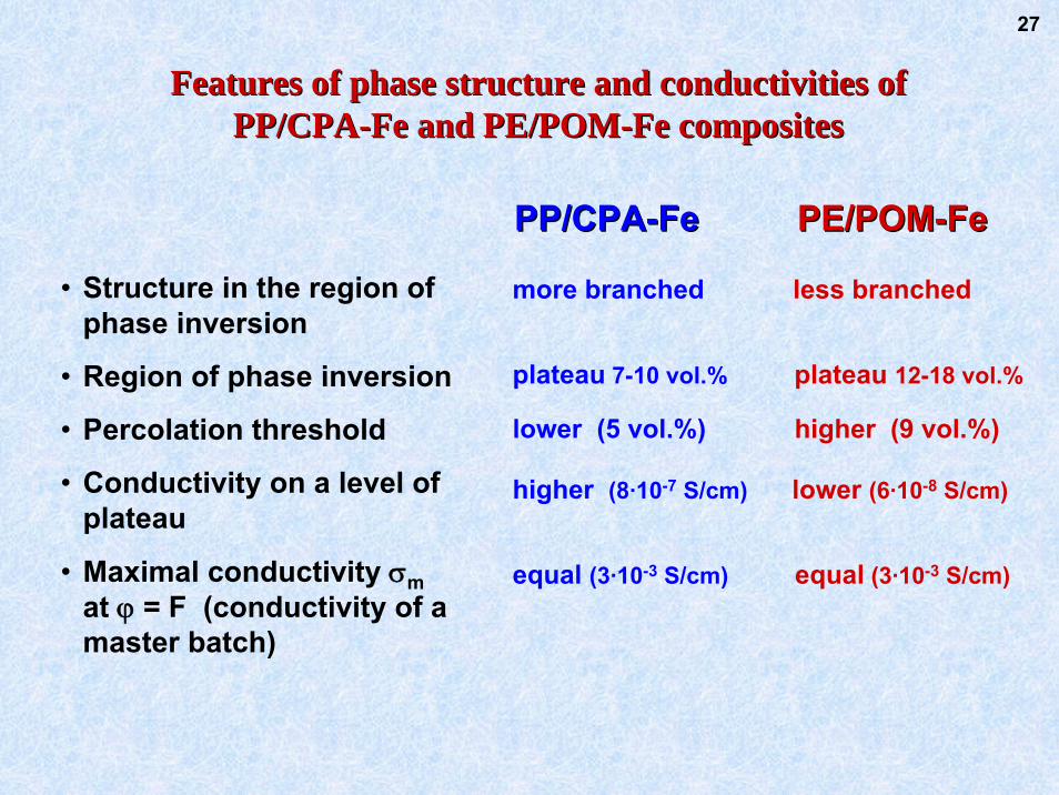
PP/CPAPP/CPA--FeFe PE/POMPE/POM--FeFe

• Structure in the region of phase inversion

• Region of phase inversion

• Percolation threshold

• Conductivity on a level of plateau

• Maximal conductivity σmat ϕ = F (conductivity of a master batch)

more branched less branched

plateau 7-10 vol.% plateau 12-18 vol.%

lower (5 vol.%) higher (9 vol.%)

higher (8·10-7 S/cm) lower (6·10-8 S/cm)

equal (3·10-3 S/cm) equal (3·10-3 S/cm)

Features of phase structure and conductivities of Features of phase structure and conductivities of PP/CPAPP/CPA--Fe and PE/POMFe and PE/POM--Fe compositesFe composites

28

Temperature, 0C

Expa

nsio

n / D

efor

mat

ion,

L, %

-1

0

1

2

3

0 40 80 120 160 200

100ПЭ78PE/15POM-7Fe62PE/26POM-12Fe53PE/32POM-15Fe28PE/49POM-23Fe68POM-32Fe100POM

Tm POMTm PE

Expa

nsio

n / D

efor

mat

ion,

L, %

-1

1

3

5

0 40 80 120 160 200

100PP80PP/13CPA-7Fe71PP/19CPA-10Fe57PP/28CPA-15Fe20PP/52CPA-28Fe65CPA-35Fe100CPA

Temperature, 0C

Tm PP

Tm CPA

• In the region of phase inversion the systems PP/CPAPP/CPA--FeFe andand PE/POMPE/POM--FeFehave two peaks of Tm which correspond to the melting point of each polymer phase.

• The slope of TMA curves depends on the composite composition for the system PE/POMPE/POM--FeFe whereas for the system PP/CPAPP/CPA--Fe Fe slope is equal for all compositions.

Thermomechanical analysis (TMA) of PP/CPAThermomechanical analysis (TMA) of PP/CPA--Fe Fe and PE/POMand PE/POM--Fe composites Fe composites

29

0

1

2

3

4

0 10 20 30 40Filler content, ϕ, %

α⋅1

04, 0

C-1


PE/POMPE/POM--Fe Fe systemsystem• Coefficient of thermal expansion αundergoes a jump in the region of phase inversion 12-18 % of Fe.• In the region 1 the values of α equal to the α of PE (αPE = 3.10·10-4 0C-1).•In the region 3 the values of α equal to the α of POM-Fe (αPOM-Fe =1.08·10-4 0C-1).

PE/POMPE/POM--Fe Fe systemsystem• The change of the composite composition does not influence on the value of α.•It is a result of equality of the α for polymer phases (PP and CPA-Fe): αPP = 1.80·10-4 0C-1,αCPA-Fe = 1.78·10-4 0C-1.

0LTL⋅

=ΔΔα

Coefficient of thermal Coefficient of thermal expansionexpansion

ΔL/ΔT is a slope of TMA curve; L0 is the initial size of sample.

Thermal expansion of PP/CPAThermal expansion of PP/CPA--Fe and PE/POMFe and PE/POM--Fe Fe composites composites

30

•The regions of phase inversion are different:

- for PP/CPAPP/CPA--FeFe system the region of phase inversion is less extended and shifted to low content of CPACPA;

- for PE/POMPE/POM--FeFe system this region is wider and located at comparable content of polymer phases PEPE and POMPOM.

0

10

20

30

40

0 20 40 60 80 100

Content of CPA (POM) in polymer matrix, vol.%

Con

tent

of F

e in

com

posi

te, v

ol.%

PP/CPAPP/CPA--FeFe

PE/POMPE/POM--FeFe

region of phase inversion

Region of phase inversion:

2929--50 POM50 POM in the polymer matrix1212--20 CPA20 CPA in the polymer matrix

• Relationship between content of filler in the polymer blend and the composition of polymer matrix.

Regions of phase inversion in PP/CPARegions of phase inversion in PP/CPA--Fe and Fe and PE/POMPE/POM--Fe composites Fe composites

0 0.25 0.5 0.75 1

η EPR

/ηPP

(200

0 C, γ

= 5.

5 s-1

)

MFI

PP (P

E)/M

FIC

PA(P

OM

)(1

90 0 C

, P=2

.16

kg)

101

100

10-1

Weight fraction of PP

Continuous EPR phase

Continuous PP phase

Co-continuous phase

PE/POMPE/POM--FeFe

PP/CPAPP/CPA--FeFe

31

D. Romanini, E. Garagnani, E. Marchetti. In: Martuscelli E., Marchetta C., editors. New polymeric materials. Reactive processing and physical properties. Utrecht: VNU Science Press, 1987, p. 56-87.

• Intervals of phase inversion of composites PE/POMPE/POM--FeFe and PP/CPAPP/CPA--FeFe were superimposed on the plot for EPR/PP system.

• In spite of using the ratio of MFIsinstead of ratio of viscosities the intervals of phase inversions for the EPR/PP system and for the PE/POMPE/POM--FeFe and PP/CPAPP/CPA--FeFecomposites are in good agreement.

Ratio of viscosities for PE/POMPE/POM--FeFe and PP/CPAPP/CPA--FeFecomposites:

MFIPP/MFICPA = 4.2·10-2

MFIPE/MFIPOM = 1.5·10-1

Influence of rheology on phase inversion in Influence of rheology on phase inversion in polymer blendspolymer blends

Influence of Influence of rheologyrheology on phase inversions in on phase inversions in polymer blendspolymer blends

32

- the higher is difference between viscosities of polymer phases, the narrower is the region of phase inversion and more shifted to the smaller content of low viscous polymer phase.

MFI

PP (P

E)/M

FIC

PA(P

OM

)(1

90 0 C

, P=2

.16

kg)

0 0.25 0.5 0.75 1

η EPR

/ηPP

(200

0 C, γ

= 5.

5 s-1

)

101

100

10-1

Weight fraction of PP

Continuous EPR phase

Continuous PP phase

Co-continuous phases

Continuous POM-Fe phase

Continuous PE phase

PE/POMPE/POM--FeFe

Continuous CPA-Fe phase

Continuous PP phasePP/CPAPP/CPA--FeFe

11

2

2

1 ≈×ϕϕ

ηη

• The rule for the point of phase inversion was calculated as well :

• These data (on the example of PE/POMPE/POM--Fe Fe andand PP/CPAPP/CPA--Fe Fe composites) composites) display the peculiarities of phase behavior:

D. Romanini, E. Garagnani, E. Marchetti. In: Martuscelli E., Marchetta C., editors. New polymeric materials. Reactive processing and physical properties. Utrecht: VNU Science Press, 1987, p. 56-87.

G.M. Jordhamo, J.A. Manson, L.H. Sperling. Polym. Eng. Sci., 1986, 26, 517-524.

EVOH - copoly(ethylene-vinyl-alcohol) with 32 and 38 mole percent ethylenePolymer blend EVOH / CoPA-6/6.9

Polymer blends for the food packaging materialsPolymer blends for the food packaging materials

• The value of permeability relatively to different gases: oxygen, carbon dioxide, water vapor are very important for the food packaging materials.

• Using of polymer blends allows to regulate the diffusion properties of film material.

• Rate of gas diffusion depends on phase morphology of polymer blend.

Y. Nir, M. Narkis, A. Siegmann. Polym. Networks Blends, 1997, 7, 139-146.

33

Materials:

Filler content

log

Res

istiv

ity

ϕc

log

Res

istiv

ity

Ts Temperature

PTC effect in conductive polymer systemsPTC effect in conductive polymer systems

• During heating the deconnexion of the percolating network occurs due to the matrix thermal expansion. This effect is reversible.

• Filled polymer is converted from conductive to nonconductive state.

• Ts – sweaching temperature for conductive/nonconductive states.

34

G. Boiteux, Ye.P. Mamunya, E.V. Lebedev, C. Boullanger, A.Adamczewski,P. Cassagnau, G. Seytre. Synthetic Metals, 2007, 157(24), 1071-1073.

thermistances

H.M. Zeng, Y.H. Hou, H.B. Zhang. Polym. Eng. Sci., 1999, 39, 1678-1688. (Scheme),

Z. Zhao, W. Yu, X. He, X. Chen. Mater. Lett., 2003, 57, 3082-3088.

35

PTC effect in filled polymers and polymer blendsPTC effect in filled polymers and polymer blends

(PVDF-CB)

Parameters of PTC dependence

Use the polymer blend as the polymer matrix instead of the individual polymer eliminates NTC effect.

Thank you Thank you for your for your

attention !attention !

electrical properties and structure of … mamunya - lecture2.pdf · structure of polymer...

Documents