electrical engineering and industrial it
TRANSCRIPT

EELLEECCTTRRIICCAALL EENNGGIINNEEEERRIINNGG AANNDD IINNDDUUSSTTRRIIAALL IITT
SSeemmeesstteerr 33
AAUUTTOOMMAATTIICC CCOONNTTRROOLL EENNGGIINNEEEERRIINNGG
22nndd SSeerriieess
2020 – 2021

Second series
A7 - PI regulation of an industrial climatic chamber
A8 - Time and frequency analysis of a car suspension model under Matlab – Part 1
A9 – Time and frequency analysis of a car suspension model
under Matlab – Part 2 A10 - Feedback-based PI closed-loop speed control A11 - Feedback-based PI closed-loop position control A12 - PI regulation of a hydraulic process

I.U.T. GE II Bordeaux 2nd Year AUTOMATIC CONTROL ENGINEERING PRACTICAL ASSIGNMENTS (PA) (AU3)
A7 PI REGULATION OF AN INDUSTRIAL
CLIMATIC CHAMBER
1 - Aim The aim is to determine the setting parameters for the controller on the industrial climatic chamber whose analysis in PA A1 in the first series allowed for the determination of a transfer function. An experiment will be carried out in order to assess the performance of the settings applied to the controller.
2 – Presentation of the equipment A DV 30 CLIMATIC CHAMBER manufactured by Sécasi Technologies (see figure 1) is used. It consists of an externally insulated chamber in which heating and refrigeration are generated by two energy sources.
Figure 1 – Photograph of the climatic chamber
It has a capacity of 30 liters and the temperature may vary between -40°C and +150 °C; it is controlled by an industrial controller and the following components are mounted above the chamber door: - on/off switch for the chamber - on/off switch for the refrigeration unit - EUROTHERM industrial controller

PI regulation of an industrial climatic chamberA 7
2
- manual override button for heating - manual override button for refrigeration - DIN socket (25-pin) for digital communication - BNC socket delivering a signal (0 / 10 volts) reflecting the internal temperature - mains power socket for powering the flatbed plotter - thermostat for temperature limitation
3 – Eurotherm controller
3.1 - Definition
The controller's function is to calculate a control signal u(t) based on the error t between the output s(t) and the set point e(t). u(t) u(t) is calculated on the basis of the following relationship
))(1
)(.()( dttTi
tKtu
3.2 - General points
a) Keypad There are six keys that perform the following functions, from left to right on the photograph in figure 2: - Select (or fast scroll) - Run - Automatic / Manual - Decrement - Increment - Scan
Figure 2 – Photograph of the front of the Eurotherm controller b) Display

PI regulation of an industrial climatic chamberA 7
3
When powered on, the controller displays its model number – 902S – for a brief moment on the central part of the display (large-format 7-bar characters), followed by the temperature measured inside the chamber m(t) in °C. The letter (W) appears on the bottom left-hand side, followed by the temperature setting c in °C (small-format 7-bar characters), which is adjusted via the increment, decrement and fast scroll keys. Press the Scan key to display the letter (Y) which indicates the output power between + or - 100%. Press the Scan key to display the set point value again.
3.3 - Programming the EUROTHERM industrial controller
a) Accessing the lists Scroll down the main menu by pressing and holding the Scan key for 1 s. Choose the rEGL (REGULATOR) menu by repeatedly pressing the Scan key Never access the other menus List of settings available to the operator: Pb Proportional band expressed as a % ti Integral action time expressed in seconds rES Manual reset (do not change) td Derived action time expressed in seconds None of the other settings should be modified, under any circumstances cbL Holdback (upper threshold) [0.0] cbL Holdback (lower threshold) [NO] HL Output 1 limitation as a % [100%] HC Cycle time of output 1 in s [10 s] Cr Relative gain of output 2, Pb (output 2) = Pb / Cr [1] CL Output 2 limitation as a % [-100 %] Cc Cycle time of output 2 in s [10 s] db Deadband output 1 - output 2 (% Pb) [0.0] Definition: The proportional band Pb is the variation, as a percentage, of the controller input required to obtain an output variation of 100%. The relationship between the gain K and the proportional band Pb expressed as a % is: K = 100 / Pb The deadband db is the distance separating the two proportional bands (inverse output hot and direct output cold); it may vary between -5 and +5% of the value of Pb. b) Programming the parameters Choose the parameter to be modified from the rEGL (OPERATOR) menu Press the key (decrement or increment) to modify a parameter; press both keys simultaneously to change the parameters quickly (fast scroll and decrement or increment).

PI regulation of an industrial climatic chamberA 7
4
Press the Scroll key to return to the permanent display. Press the Select key to return to the main menu. NB. The display duration is 15 s; the main menu will then reappear if no keys are pressed.
4 – Transfer function of the climatic chamber
The identification carried out in the 1st series (A1) was used to obtain the open-loop transfer function of the climatic chamber.
p
eGsyspG
p
.1.)(
.
We shall now consider the numerical values of the parameters of this transfer function.
Gsys = 1.5 = 40 s = 3600 s;
The Matlab software and the script described in the subject of TP A1 can be used to obtain
the Bode diagrams of the transfer function G(p).
5 - Calculation of parameters for the PI controller
This involves calculating the parameters of a PI controller whose frequency response at reduced angular frequency is given in Annex 1, according to the method described in the Teaching Assignment.
1. Using Matlab, in the Bode area, plot the frequency response of G(j).
2. The following relationship is given for the controller: ))(1
)(.()( dttTi
tKtu
On the basis of the temporal relationship, extrapolate the transfer function of the controller C(p)=
U(p)/(p)
3. Calculation of a P.I.
Where 0 is the angular frequency for which the corrected open loop has a modulus of 1. For
this angular frequency, the argument of the PI controller is set at -20°. The aim is to obtain a phase margin of = 45°. Determine the transfer function of the controller C(p).
4. Demonstrate that this type of controller asymptotically rejects the "step"-type disturbance shown by the ambient temperature in the block diagram above. For the demonstration, c = 0.

PI regulation of an industrial climatic chamberA 7
5
6 – Operation 6.1 – Implementation of controllers
For the first controller obtained above, apply (using the V. I. Labview Enceinte_climatique.VI available on the desktop) the parameters Pb and Ti to the controller.
After the temperature has reached the value of 95 °C, i.e. after approximately 15 min:
- record the temperature variations in the chamber in response to a setting of 100°C, - state your conclusions regarding the results obtained.
- Using Matlab, plot the results of the open-loop system on a Nichols plot and from them, extrapolate the phase margin and gain margin. Also give the static gain of the closed loop.
- Check whether there is an overvoltage. If there is an overvoltage, give the modulus of the corrected open loop for this particular point and from it, extrapolate the overvoltage ratio.
6.2 - Automatic calculation of the controller parameters To launch the automatic calculation of the parameters by using the self-regulating algorithm:
- close the V. I. Labview used in the first part; - leave NO as the value of Td; - launch the automatic calculation phase, by referring to the method described in Annex 3. - At the end of the calculation, record the new parameters Pb and Ti and compare them with the previous values. - Launch the V. I. Labview Enceinte_climatique.VI available on the desktop and implement the parameters Pb and Ti found before. Launch the V. I.
- Save the temperature variations in the chamber again in response to a new variation in the setting of ± 10°C around 100 °C. - Compare with the previous results and state your conclusions.
__________________________

PI regulation of an industrial climatic chamberA 7
6
ANNEX: Using the "Self-regulating" function on the Eurotherm 902 controller
2.2: Automatic method: using self-regulating and self-adapting algorithms The controller possesses two parameter calculation algorithms: self-regulating and self-adapting. The self-regulating algorithm is designed to calculate the parameters during installation. Once the loop is in service, the self-adapting algorithm adjusts the PID values according to the changes in operating conditions. 2.2.1 Selection of the self-regulating parameter
Go to the Regulator (Régleur) list: REGL (InSI) (See Section 2 - §3) Check that the parameters tI and Pb are different from OFF Set cbL and cbh to OFF Set Cc-10 seconds if the output is modulated (Relay – Logic – Triac) The algorithm can be selected either via a logic input configured for this purpose, or by
simultaneously pressing ∧ and ∨ when Ar (St) is displayed in the OPERATOR (OPERATEUR): OPEr menu
When the self-regulating algorithm is validated, the letters ST (AT) are displayed in the top right-hand corner of the screen; the set point is displayed and the parameter W (SP) flashes for one minute, during which time the set point can be changed. After this time, the letters ST (AT) flash and the set point can no longer be changed. The controller then runs through an operating sequence in on-or-off mode which allows it to calculate the regulation parameters; when the calculation is finished, the letters ST (AT) go off. The self-regulating calculation can be interrupted at any time by simultaneously pressing ∧ and
∨ when Ar (St) is displayed in the OPERATOR (OPERATEUR): OPEr menu.

A8 & A9 TIME AND FREQUENCY ANALYSIS OF A
CAR SUSPENSION MODEL UNDER MATLAB
Requirements :
‐ Linear ordinary differential equations ‐ Laplace transform ‐ Frequency analysis (Bode diagram)
Objectives : Let a car suspension system be considered, we will:
‐ Achieve temporal and frequential analysis for different road profile types ‐ Design a simple controller of the proposed system (active car suspension)
I. Introducing car suspension system
The car suspension is composed of four identical systems between the car chassis and each shaft of the wheel, see Fig. 1 for more details. It allows two different main functions :
‐ Safeguard permanent grip of the wheels on the road and directional stability of the car in all circumstances. It needs that motor; directional and brake efforts are correctly transmitted.
‐ Safeguard car passenger security by allowing the wheels to follow the road profiles irregularities and by attenuating important chassis displacements.
Fig. 1: Illustration of car suspension elements

The kinematic model of a car suspension is also introduced in Fig.2. Each of the four (identical) elements of a car suspension is now detailed as follows:
‐ Tire and its associated damper (rubber of the tire) ‐ Helicoidal spring of a suspension ‐ Damper of oil piston tubular suspension
Fig. 2: Kinematic model of a car suspension
In order to simplify the study, we will uniquely consider of car suspension quarter model (here the tire/damper set), by restricting vertical displacement experienced by this latter. Furthermore, the dynamical couplings between the four tire/damper sets are also not considered in this study.
II. Suspension quarter model a. Damper/tire suspension model
This model is composed of a suspended mass modeling the car chassis, which rests
through the suspension on the wheel mass in contact with the road through the tire, see Fig. 3. The suspension is modelized by a spring/damper equivalent system in parallel. The wheel (including the tire and its associated deformations) is also modelized by spring/damper set equivalent system in parallel. Here, it is considered that spring stiffness and damping coefficient numerical values are higher than those of the suspension.

Fig. 3 : Suspension quarter damper/tire model By applying the dynamical fundamental principle (in translation), the model is described by the following differential equations:
𝑚𝑑 𝑧𝑑𝑡
𝑘 𝑧 𝑧 𝜇𝑑𝑧𝑑𝑡
𝑑𝑧𝑑𝑡
1
𝑚𝑑 𝑧𝑑𝑡
𝑘 𝑧 𝑧 𝜇𝑑𝑧𝑑𝑡
𝑑𝑧𝑑𝑡
𝑘 𝑧 𝑧 𝐹 2
where ‐ 𝑧 : Chassis height in reference to the resting position ‐ 𝑧 : Tire height in reference to the resting position ‐ 𝑧 : Road height ‐ 𝑚 : Mass quarter of the car chassis ‐ 𝑚 : Tire mass ‐ 𝑘 : Spring stiffness of the damper ‐ 𝜇 : Viscous damping coefficient (or viscous friction coefficient) ‐ 𝑘 : Equivalent tire stiffness ‐ 𝐹 : Equivalent tire damping force
In the sequel, let consider 𝐹 0.
b. Simplified damper (alone) model Given that the wheel has numerical values of spring stiffness and damping coefficient
higher than those of suspension, then we consider a second model describing uniquely the chassis and damper behavior, see Fig.4 for more details.

Fig. 4: Suspension quarter model considering damper alone By applying the dynamical fundamental principle (in translation), the differential equation related to the model describing the variations height level of the chassis (zc) according to road height level (zs) is given as follows:
𝑚𝑑 𝑧𝑑𝑡
𝑘 𝑧 𝑧 𝜇𝑑𝑧𝑑𝑡
𝑑𝑧𝑑𝑡
3
Designing a car suspension necessitates to isolate car chassis from vibrations of road irregularities by an adequate filtering process and allowing also that motor, directional and brake efforts are correctly transmitted. However, other parameters need to be guaranteed as the vibration behaviour related to physiological human behaviour, in particular by limiting vertical acceleration for specific frequencies to maintain a good comfort level for passengers. Human body is able to tolerate vertical accelerations levels that are different according to specific frequencies under consideration, as depicted in Fig. 5. It is characterized in the norm AFNOR E90‐400. Indeed, it exists a motion sickness zone (zone A) and a vibration discomfort zone (zone B). These shaded zones depend on the trip duration: the limits for 30 min, 2h et 8h are indicated in dotted lines.

Fig. 5: Human physiology tolerance norm according to vertical vibrations AFNOR E90‐400
III. Temporal and frequential analysis of car suspension
a. Suspension model analysis In the sequel, by assuming that initial conditions are null, based on the differential equations (1), (2) et (3) in Laplace domain, by adopting 𝑍 𝑝 ℒ 𝑧 𝑝 , 𝑍 𝑝 ℒ 𝑧 𝑝 and 𝑍 𝑝 ℒ 𝑧 𝑝 we deduce:
‐ Damper/tire suspension model case (homework if not enough time in practical session):
𝐻 𝑝𝑍 𝑝𝑍 𝑝
𝑎 𝑎 𝑝𝑏 𝑏 𝑝 𝑏 𝑝 𝑏 𝑝 𝑏 𝑝
4
where each parameter of the transfer function 𝑎 , 𝑏 où 𝑖 𝜖 0,1 , 𝑗 𝜖 0, … ,4 , is given as a
function of system parameters (𝑚 , 𝑘, 𝜇, 𝑚 , 𝑘 such that 𝑎 𝑘 , 𝑎 . , 𝑏 𝑘 , 𝑏
𝜇, 𝑏 𝑚 , 𝑏 𝑚 𝑚 , 𝑏 .
‐ Damper (alone) suspension model case:
𝐻 𝑝𝑍 𝑝𝑍 𝑝
1 2𝜁𝜔 𝑝
1 2𝜁𝜔 𝑝
𝑝𝜔
5
where each parameter (𝑤 , 𝑧 of the transfer function is expressed as follows:

𝜔 𝑘 𝑚
𝜁 𝜔𝜇
2𝑘𝜇
2 𝑘𝑚
𝜇 2 𝑘𝑚 𝜁 Considering the transfer function complexity 𝐻 𝑝 , we will use the transfer function 𝐻 𝑝 for the rest of the study. The following parameters are now used in the sequel:
𝑚 250𝑘𝑔, 𝑚 35𝑘𝑔, 𝑘 15000𝑁. 𝑚 , 𝑘 175000𝑁. 𝑚 Q1: Under Matlab, in a new script with dedicated format .m, program
‐ All the values of parameters used in 𝐻 and 𝐻 ‐ The two transfer functions 𝐻 and 𝐻 with the help of Matlab function « tf » ‐ The plot of the two bode diagrams 𝐻 and 𝐻 on the same graphic, with the help
of function « bode » Q2:
a) On the plot of the two obtained Bode diagrams, what is the frequency band on which the two models are sufficiently closed to be considered as relatively similar?
b) What kind of hypothesis is assumed if we conserve the model with the associated transfer function 𝐻 ?
c) What is the resonance pulsation and its associated amplification gain? (give the numerical values obtained for H1 et H2 and make a comparison)
N.B: Always keep in mind that a model by definition is only a conceptual simplified approximation of the reality. Q3: How will evolve the plots of the bode diagrams in case of a worn suspension with a parameter set‐up to μ 1,8. 10 N.s.m‐1? What will be the consequences for the vehicule behaviour? Q4: How will evolve the plots of the bode diagrams in case of a heavy load with four passengers and their luggage and with a parameter set‐up to m 325kg?
b. Suspension response for different road profiles We would like to simulate a road level rise height of 5cm (stair type), as depicted in Fig. 6.

Fig. 6: Suspension experiencing a stair type profile road
Q5: What kind of input signal allows to generate the considered road profile? Q6: In Simulink environment, program and parametrize suspension temporal simulation in response to road profile as follows:
The following parameters are adopted:
‐ The road level rise height is considered at 1s after the simulation beginning and a time simulation horizon of 3s is set‐up.
‐ A fixed sampling time is set‐up at 0.001s and the « solver » method used is the Runge Kutta of fourth order 4 (menu Simulation / Model Configuration Parameters)
‐ An « array » structure type as format recording for the blocs « To Workspace » is considered for t, u, y1, y2.

Q7: Plot in the same figure the input and output of the transfer functions 𝐻 , 𝐻 . Determine also the response time of 5% and the first overtaking rate. Q8: Evaluate the transfer functions poles for 𝐻 , 𝐻 with the help of Matlab function « pole ». Plot the poles in the complex plan with the help of function « pzmap ». Are the transfer functions stable? What is the influence of the imaginary part of poles on the suspension temporal response? Q9: Do again the questions Q6‐Q7 for the two cases considered in questions Q5 et Q6.
Q10: By recalculating the coefficient value 𝜇 2 𝑘𝑚 𝜁 for 𝜁 1 and 𝜁 1.5, do again the previous questions? Superimpose all the results on the same figure. What could you conclude? Now, we consider a car moving at a constant speed value 𝑉 in the horizontal direction �⃗�, experiencing a road profile modeled by a sinusoidal input signal varying through the time as follows
𝑧 𝑡 𝐴𝑐𝑜𝑠 𝑥 𝑡 𝐴𝑐𝑜𝑠 𝑤𝑡 (6)
where 𝜆 denotes the distance between two maxima of the twisty road profile. An illustration is given in figure 7.
Fig. 7: Suspension experiencing a periodic road profile
The suspension response to the periodic road profile is written as:
𝑧 𝑡 𝐴|𝐻 𝑗𝑤 |cos 𝑤𝑡 𝑎𝑟𝑔 𝐻 𝑗𝑤 (7)
where |𝐻 𝑗𝑤 | and 𝑎𝑟𝑔 𝐻 𝑗𝑤 correspond respectively to the modulus (warning modulus
is not in dB!) and to the phase of the transfer function 𝐻 𝑗𝑤 . Q11.a) Determine the expression of 𝑧 𝑡 .
b) Given that A = 5cm and the cosine function is increased by a constant, deduce the absolute value expression maximum vertical acceleration amplitude 𝑧 experienced by the passengers.

c) With the help of Matlab software and the proposed program below that you will have to comment line by line, calculate the maximal acceleration values for the frequency band (warning, here in Hertz) of 0.1Hz to 10.1Hz.
A=0.05 ; f=0.1: 1:10.1 ; w=2*pi*f ; [mag,phase,wout]=bode(H2,w) ; for k=1:length(mag) temp_mag(k)=mag(1,1,k); end acc_max=(w.^2).*A.*temp_mag; [f’ acc_max’]
d) Referring to figure 5 and supposing that car passengers are experiencing the twisty road profile under study, are the performance level according to the damping effect level of vertical acceleration satisfied for a trip duration of 2 hours long? In order to improve the suspension performance level, it is proposed to study active suspension. In the sequel, we keep the value initially set‐up at 𝜁 0.707.
c. Active suspension analysis
An active suspension needs to have a vertical accelerometer sensor on the chassis, as depicted in figure 8. The measure obtained from the sensor on the chassis, denoted as 𝑦 𝑡 , is used as an input of a controller, in order to design control law 𝑢 𝑡 . In comparison of a classical suspension for which the spring/damper set is linked to a chassis position denoted as 𝑧 𝑡 , the active suspension superimposes a position modification to the chassis, denoted as 𝑧 𝑡 . This modification results of the supplementary force application obtained with the help of an actuator positioned to this effect and controlled by 𝑢 𝑡 . The active chassis position 𝑧 𝑡 (with active suspension) results by superimposing the contributions described previously: 𝑧 𝑡 𝑧 𝑡 𝑧 𝑡 in the temporal domain.

Fig. 8 : Suspension active
In the sequel, the following transfer functions are used:
𝑍 𝑝 𝑍 𝑝 𝑍 𝑝
𝐻 𝑝𝑍 𝑝𝑍 𝑝
𝐻 𝑝𝑍 𝑝𝑈 𝑝
𝐶 𝑝𝑈 𝑝𝑌 𝑝
𝑈 𝑝𝐸 𝑝
𝐷 𝑝𝑌 𝑝𝑍 𝑝
A block‐diagram describing an active suspension is now given as follows:
Q12: a) Recall what do the different blocks and elements represent in the closed‐loop scheme dedicated to the car suspension.
b) Give the transfer function expression in closed‐loop 𝐺 𝑝 of active suspension.
c) Interpret physically the set‐value 𝑦 equal to 0.
𝐻 𝑝
𝐻 𝑝 𝐶 𝑝 𝐷 𝑝 𝑦 0 𝑧 𝑦 𝑧 𝑢 𝑧
𝑧
𝑧
++
- +
𝑒

Q13: a) Give the expression of the transfer function 𝐷 𝑝 , knowing that the output
corresponds to the measure assumed to be unnoisy for chassis acceleration and the input is the adjusted chassis position.
b) The block‐diagram scheme of the controller is given in figure 8 hereafter. Give the expression of the transfer function 𝐶 𝑝 . What is the classical controller structure that you recognize?
Fig. 8: Block‐diagram scheme of the controller 𝐶 𝑝
c) Assuming that
𝐻 𝑝1 2𝜁
𝜔 𝑝
1 2𝜁𝜔 𝑝
𝑝𝜔
𝐻 𝑝1
1 2𝜁𝜔 𝑝
𝑝𝜔
Demonstrate that the literal expression of the transfer function in closed‐loop can be written as follows:
𝐹 𝑝𝑍 𝑝𝑍 𝑝
1 2𝜁𝜔 𝑝
1 2𝜁𝜔 𝐶 𝑝 1
𝜔 𝐶 𝑝
d) Assuming that the transfer function obtained can be written under the canonical form
as follows
𝑍 𝑝𝑍 𝑝
1 2𝜁𝜔 𝑝
12𝜁𝜔 𝑝 1
𝜔 𝑝
where 𝜔 and 𝜁 correspond to the proper pulsation and to the damping factor of the close‐loop system, demonstrate that
𝐶1
𝜔1
𝜔
𝐶2 𝜁 𝜁
𝜔
e) With the help of Matlab, determine the numerical values of 𝐶 and 𝐶 knowing that
we would like to get 𝜔 5𝑟𝑎𝑑/𝑠 and 𝜁 1.
𝐶 1𝑝
𝑈 𝑝 +
+𝐸 𝑝
𝐶

f) Under simulink environment, change the block‐diagram scheme such that it is able to simulate the closed‐loop of the suspension in one block « Transfer Fcn » for a road level rise height of 5cm in input. Compare the obtained results for passive and active suspension. Conclude.
Q14: Modify the parameters 𝜔 et 𝜁 for different values and observe the associated active suspension behaviours. Superimpose results set on the same figure. Conclude. Q15: Implement again into Simulink the active suspension, this time not as one single block "Transfer Fcn" as asked in question Q13f, but by reproducing the complete closed‐loop block‐diagram in question Q12 including the accelerometer sensor. This latter has a limited bandwitch considered as
𝐷 𝑠𝑠
1 𝜏𝑠
With 𝜏=1ms (notice that the transfer function 𝐷 𝑠 becomes "realizable"). Compare the temporal responses obtained from the active and passive suspension models and conclude.
g) Compare under Matlab the passive suspension bode diagrams studied in part II.a and those from active suspension. What is the influence of close‐loop control scheme on the proper pulsation? What are the amplified frequencies for the active suspension case? Conclude.
Q16: For the different values for parameters 𝜔 and 𝜁 in QE, superimpose the bode diagrams set of active and passive suspension on the same figure. Conclude. Conclude your practical work session by summing‐up the methodological elements necessary:
‐ To achieve a temporal and frequential analysis of suspension system ‐ To design a controller for suspension system

Annex 1 : Laplace transform


I.U.T. GE II Bordeaux 2nd Year AUTOMATIC CONTROL ENGINEERING PRACTICAL ASSIGNMENTS (PA) (AU3)
A10 FEEDBACK-BASED PI CLOSED-LOOP SPEED
CONTROL
Figure 1 - Mechanical unit on the breadboard
Brake magnet
Tachogenerator
Turn potentiometer
Output shaft
Reduction gear

2/6
1. Aims The aim is to study the principle of the closed-loop control of the speed of a direct-current
motor, in addition to the benefits of using the proportional and integral regulator in a closed speed control loop.
2. Prerequisites Before starting the session, it is essential to have read through and worked on the course
handouts (the part on regulator design – P and PI Regulators) and your notes made during the lectures.
3. Theory part See the theory part in the Teaching Assignment (TA) workbook.
4. Practical part with report
A photograph of the analog unit on the breadboard is presented in figure 4.
Figure 2 - Photograph of the mechanical unit on the breadboard
The proportional controller consists of the ("error amp.") comparator and the P1
potentiometer (see figure 5). The gain is adjusted via the choice of degenerating resistors for the
comparator and via the adjustment of the P1 potentiometer.
The controller is therefore reduced to a real number C0 representing the gain of the
comparator and of the potentiometer P1.
In addition, several voltages can be applied as input settings (see bottom left-hand side
underneath the potentiometer P3):
Direct voltage of 10 V which can be reduced using the P3 potentiometer,
Triangle-wave voltage of 10 V that can be reduced using the P3 potentiometer.
U
E1 (non-inverting input)
E2 (inverting input)
Amp. offset setting
Potentiometer P1
Differential amplifier
i
o
Potentiometer P3

3/6
Triangle wave voltage, not used in this PA.
Figure 3 – Diagram of the breadboard used to create the controllers
4.1 Closed-loop control with a proportional (P) controller – Static analysis
1. Perform the wiring for figure 3 on the breadboard in figure 5, where: a. The set point r(t) is a continuous voltage of 2 V. The exact measurement of r(t) is
carried out by moving the "RPM/DVM" switch to "DVM" and by wiring the potentiometer P3 to the "DVM" input. The +10 V continuous voltage is the P3 input.
b. C0 , the controller gain, is the combination the comparator gain, with a degenerating resistor of 1M, and of the potentiometer P1 set at 50%. Calculate the value of C0.
c. Remember to connect the output of the potentiometer P1 to the inverting input of the amplifier.
2. Measure the image of the speed v2(t) at the output of the tachogenerator.
3. Evaluate the error signal (t), and then measure it.
4. Measure the rotation speed (t) of figure 2 in rpm. To this end, move the "RPM/DVM" switch to the "RPM" position.
5. According to the measurements, repeat the calculation of the tachogenerator gain in order to adjust it.
6. Now set the P1 to 100%, repeat Q. 1.b, 2 and 3, and then state your conclusions.
7. Braking torque is added by lowering the electromechanical brake lever, which has the effect
of changing the disturbance c(t) in figure 3. Repeat the preceding measurements (Q.1.b, 2 and 3) in each of the two cases for P1 at 50% and P1 at 100%. State your conclusions.

4/6
4.2 Dynamic analysis The fixed set point input is now replaced by a variable pulsed input. After raising the brake magnet lever, via the potentiometer P3, wire the set point input of the comparator to the square-wave signal generator output. Set the frequency at 0.1 Hz, and the amplitude at ± 2 V.
8. For P1 = 50%, on the oscilloscope, view the set point r(t) and speed (V2) signals and print
out the curves. Measure the settling time to obtain 10% of the final response.
9. For P1 = 100%, repeat the same operation and then state your conclusion. 4.3 Closed-loop control with a (PI) controller – Static analysis
A proportional and integral controller can be created by the electronic circuit in figure 6
Figure 4 – Proportional and integral controller
10. Calculate the transfer function of this controller according to the value k of the voltage
divider of the potentiometer P5 and show that the transfer function of a PI has been obtained.
11. Wire the controller according to the diagram in figure 6. Adjust the gain of the "error
amp." comparator to -1 (replace the 1 Mresistor with a 100 k resistor, with negative feedback for the operational amplifier). Wire the comparator output to the controller input, via the gain adjustment potentiometer P1 set at 100%. Wire the controller output to the power amplifier input E2. P5 is set at 100%.
a. Evaluate the parameters of the PI controller obtained in this way.
12. As in Q1.a, set the set point r(t) at 2 V. With no brake applied, measure: a. The rotation speed (t) (see figure 3) on the digital display in "RPM". b. The error (t) in figure 3.
13. Repeat the same measurements with a motor brake applied and state your conclusions.

5/6
4.4 Dynamic temporal analysis
14. After raising the brake magnet lever, replace the fixed set point input with a variable pulsed input at an amplitude of 1 volt and frequency of 0.1 Hz.
15. Simultaneously view the set point r(t) and measured speed v2(t) signals on the oscilloscope.
State your conclusions. 4.5 Dynamic frequency analysis The set point signal is now a sinus-wave signal originating from the analyzer.
16. Connect the analyzer generator output to the Feedback comparator input. Connect the comparator ("error amp.") output to channel 0 of the Labview analyser (check that the cable connecting the generator to channel 1 has been removed). Connect the tachogenerator output (-UT) for the Feedback to channel 1 of the Labview analyzer.
a. On figure 3, mark the measurement points corresponding to this wiring. The measurements therefore relate to the closed-loop control forward path.
b. Plot the two Bode curves (modulus and argument) and then the Nichols locus for the system frequency response, from 0.1 Hz to 10 Hz. The generator will be programmed so that the amplitude of the sinus-wave signal is 2 V, and the offset (bias) is 3 V.
c. On the Bode curves and Nichols locus, show and measure the phase margin.
5. State your conclusions.

6/6

I.U.T. GE II Bordeaux 2nd Year AUTOMATIC CONTROL ENGINEERING PRACTICAL ASSIGNMENTS (PA) (AU3)
A11 FEEDBACK-BASED PI CLOSED-
LOOP POSITION CONTROL
Figure 1 - Mechanical unit on the breadboard
The analog automatic control engineering course presents an example of a
problem with the orientation of an antenna intended for the reception of television images relayed by satellites. The topic covered on this day concerns the creation of such a control system, using the Feedback breadboard in order to represent the operational part (mechanical unit) of a multi-directional antenna, and for the installation of a Proportional and Integral (PI) controller on the analog unit.
Brake magnet
Tachogenerator
Turn potentiometer:
Output shaft:
Reduction gear

1. Creation of a PI controller The following notations will be used hereafter: Position set point c
Reference voltage: Vc
Angular position of the output shaft: Output voltage of the position measurement potentiometer: VError signal voltage: Control voltage (power amp. input): U Offset voltage: d Angular velocity of the motor: Output voltage of the tachometer generator: V a) - Description and modeling of the controlled system
The operational part of the Feedback breadboard (mechanical unit) was described in the Automatic Control Engineering PA handout for the 1st Series.
This electromechanical part consists of: - a turn potentiometer that displays the gain set point kc
- a direct-current motor and its power amplifier (comprising a zero adjustment potentiometer), for which a model was created in a practical assignment (PA) in the 1st series, in the form of a first-order transfer function between the amplifier input voltage and the tachogenerator voltage output in the following form:
ppU
pV
4,01
8.0
;
- a gain speed reducer kred
- a potentiometer for measuring the angular position of the output shaft (representing the axis of the antenna), with gain of kmes
The associated numerical values are listed below:
• kc = kmes = 5/90 V/deg = 10/ V. rad-1
• static gain (angular speed of motor) / (amplifier input voltage) = 1740 deg.s-1.V-1 =30.46 rad.s-
1.V-1. • time constant of the 1st order model of speed/input voltage of the power amplifier = 0.4 s (see 1st series PA) • kred = 1/32. • Ktachy = 2.75 mV.r-1pm. The transfer function, which links the control signal U and the image voltage of the angular position of the output shaft whose position is to be governed by closed-loop control, is thus defined by:
pppU
pV
4,01
03.3
.
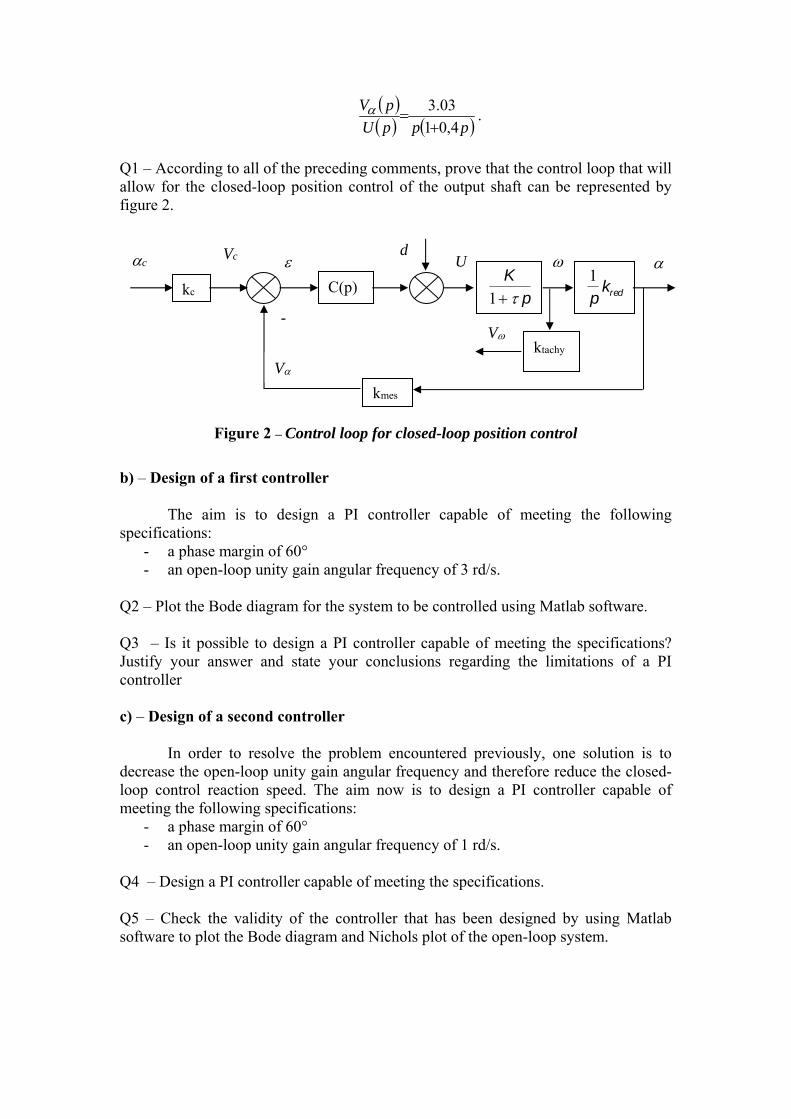
Q1 – According to all of the preceding comments, prove that the control loop that will allow for the closed-loop position control of the output shaft can be represented by figure 2.
Figure 2 – Control loop for closed-loop position control
b) – Design of a first controller The aim is to design a PI controller capable of meeting the following specifications:
- a phase margin of 60° - an open-loop unity gain angular frequency of 3 rd/s.
Q2 – Plot the Bode diagram for the system to be controlled using Matlab software. Q3 – Is it possible to design a PI controller capable of meeting the specifications? Justify your answer and state your conclusions regarding the limitations of a PI controller c) – Design of a second controller In order to resolve the problem encountered previously, one solution is to decrease the open-loop unity gain angular frequency and therefore reduce the closed-loop control reaction speed. The aim now is to design a PI controller capable of meeting the following specifications:
- a phase margin of 60° - an open-loop unity gain angular frequency of 1 rd/s.
Q4 – Design a PI controller capable of meeting the specifications. Q5 – Check the validity of the controller that has been designed by using Matlab software to plot the Bode diagram and Nichols plot of the open-loop system.
kc C(p) K
1 p
1
pkred
ktachy
kmes
c Vc U
- V
d
V

d) – Creation of the controller
A proportional and integral controller can be created by the electronic circuit
in figure 4.
Figure 2 – Proportional and integral controller
The circuit in figure 4 is situated at the bottom of the analog unit as shown by
the photograph in figure 5.
Figure 5 - Photograph of the analog unit on the breadboard
V
U (non-inverting input)
-U (inverting input)
Amp. offset setting
Potentiometer P1
Differential amplifier
Vc
V
Potentiometer P3
Controller part
Potentiometer P5

Q6 – Check that the transfer function of the circuit between the input of the potentiometer P1 and the output of the last operational amplifier in figure 4 is:
pCR
PPpC
ii
51 1 .
Q7 – Find the values of P1, P5 and Ci , in addition to the values of the resistances associated with the "differential amplifier" part of the analog unit in order to obtain the controller in question 5.
Q8 – Wire and test the control loop.
2. Temporal tests
a) - Static tests.
The potentiometer situated in the mechanical part will act as the position set
point display.
Q9– In the absence of offset voltage (adjustment potentiometer in the central
position), check that the static position error is still nil.
Q10 – Check that this static error remains nil even in the presence of offset
voltage. State your conclusions regarding the operation of the control loop
b) - Dynamic temporal tests.
The fixed set point input is now replaced by a variable pulsed input.
After setting the offset amplifier at zero (potentiometer in central position):
• Wire the set point input of the comparator to the square-wave signal
generator output via the potentiometer P3.
• Set the frequency at the minimum and the amplitude at ± 2 V.
Q11 – On the oscilloscope (Labview program available on the computer
desktop), view the set-point signals (voltage -U) and the position signals (voltage -
V), and print out the result.
3. Frequency tests
The set point signal is now a sine-wave signal originating from the Labview
frequency response analyzer, available on the computer desktop.

• Connect the analyzer generator output to the Feedback comparator input (reference voltage Vc).
• Connect the comparator ("error amp.") output to input 0 of the analyzer (check that the cable connecting the generator to channel 0 has been removed).
• Connect the position measurement output (V) for the Feedback to input 1 of the analyzer.
Q12 – On a block diagram of the closed position control loop, mark the
measurement points corresponding to this wiring. The measurements therefore relate to the closed-loop control forward path.
Q13 – Plot the Nichols locus of the system's frequency response, from 0.1 Hz
to 10 Hz. The analyzer generator shall be programmed so that the amplitude of the sinus-wave signal is 2 V, and the offset (bias) is 0 V.
Q14 – Measure the phase margin.
4. Conclusion
State your conclusions regarding the limitations of a PI controller.

I.U.T. GE II Bordeaux 2nd Year AUTOMATIC CONTROL ENGINEERING PRACTICAL ASSIGNMENTS (PA) (AU3)
A12 PI REGULATION OF A HYDRAULIC
PROCESS
1 - Preparation
Before starting the session, it is essential to have read through and worked on the course handouts (pp. 74 to the end) and your notes made during the lectures.
1.1 - Description of the process to be controlled The process studied in the framework of this tutored assignment (TA) / practical assignment (PA) was previously modeled in PA A02 (first series). As shown by the diagram in figure 1, it consists of one operational part and one control / supervision part.
Figure 1 – Process diagram
Pump P101
Measurement interfaces
Power interfaces
PC and software
Eurotherm 2408f regulator Profibus DP
link
Tank
Vessel
Valve
Level sensor
Operational part
Control / supervision part
Flow rate sensor

2/9
As shown by the diagram in figure 1, the following components of the operational part are used in the PA: - graduated vessel (reference B102) - tank (reference B101) - centrifugal pump (reference P101) - electropneumatic valve (reference V102) - ultrasound depth sensor (reference LIC102) - flow rate sensor (reference FIC 101). The operational part is controlled by Labview software via a 2408f-type industrial controller manufactured by Eurotherm. Communication between the controller and the PC is carried out using the Profibus DP protocol and via an Applicom board. Here, the power interfaces are used for powering the direct-current motor that drives the pump and the solenoid valve. The measurement interface is used for converting the information that originates from the ultrasound level sensor and the flow rate sensor into an exploitable format.
1.2 – Modeling of the process
During PA A02, it was revealed that the process described previously could be modeled by the following differential equation:
tQtQ
dt
tdhS se , (1)
where S designates the cross-section of the vessel Qe(t) designates the flow rate going into the vessel Qe(t) designates the flow rate coming out of the vessel
It was also shown that the incoming flow rate and the outgoing flow rate from tank 1 could be characterized by the following relationships:
Qe(t) = Q(U)- ah(t) and thQ ts (2)
with h: depth of water in the vessel a: coefficient determined in the previous PA : coefficient determined in the previous PA Q(U): flow rate for h = 0 in a steady state. Combining the relationships (1) and (2) creates the model that links the flow rate Q(U) to the depth of water in tank 1, i.e.
Sdh t
dtQ U ah(t) h(t), (3)
Due to the presence of the term th , the differential equation (3) is non-linear in h(t). To
linearize this equation, we shall assume that the depth of water remains approximately h0 , consequently, it can be stated that:
tHhth 0 with 0htH
and that the pump output remains approximately 0UQ (output for a command U0 which leads to a
depth of water of h0), i.e.
tqUQUQ 0 with 0UQtq .
The relationship (3) thus becomes:
tHhtHhatqUQdt
tHhdS
000
0 .
With the understanding that 2
11x
x for 1x , this gives:
0000
0
21
h
tHhtHhatqUQ
dt
tHhdS
or
Sd h0 H t
dtQ U0 q t a h0 H t h0
H t 2 h0
or also
02 h
tHtaHtq
dt
tdHS (4)
given that in equilibrium 0000 hahUQ (which shows that the incoming flow rate
offsets the outgoing flow rate). The Laplace transform of the equation (4) reveals that the depth of water and the flow rate are linked by the transfer function:
02
1
haSp
pq
pH
. (5)
When a command is applied to the pump, the output at its outlet does not become established immediately. In TP A02, it was shown that the output q(t) and the command U(t) are linked by the transfer function:
p
K
pU
pq
11 . (6)
By supplementing this analysis with several experiments that allow for the assessment of the
parameters a, , Kp and , it can be shown (see TP A02) that the hydraulic process can be characterized, around a given level, by the following type of transfer function:

4/9
0
1
21
haSpp
K
pU
pHpG
2 – Operation The PA has three aims, namely to: - compare the performance obtained using a proportional controller followed by a proportional
and integral controller, - deploy an industrial panel controller, - study one specific functionality of industrial controllers: gain scheduling.
Throughout the entire PA, configure the operational part in the following manner: - move the PLC/Controller switch on the right-hand side of the controller to Controller, - close the manual valves V103, V104, V107, V108, V109, - open the manual valves V101 and V112, - open the electropneumatic valve V102, - open valve V112 so that the red lines marked on this valve are aligned.
Refer to annex 1 for information about powering the operational part and running the supervision software.
2.1 – Proportional control 2.1.1 Controller design The industrial controller situated in the operational part allows for the deployment of a proportional gain controller Kc by setting the parameter Ti at 0 and the parameter Pb (referred to as the proportional band) at the value of 100/Kc. 2.1.2 Operation
Apply the following: Pb1=Pb2=15 and Ti1=Ti2=0 (the integral actions will then be deactivated). This can be carried out directly in the Labview window or on the controller. In the
latter case, press the button twice to reveal the "PID list" menu. Enter the menu by pressing .
Pressing the
key repeatedly gives access to the following parameters consecutively: Gsp, Pb, Ti, Td, Res, hcb, lcb, … Pb2, T2i,… (Pb, Ti correspond to Pb1, Ti1). The value of these parameters
can be modified by pressing the or buttons in order to increase or decrease their values).
Question 1 - Apply a water depth set point of 190 mm. When the level has stabilized, apply a water depth set point of 210 mm and record the changes in the level of tank 1.
Check that the set point has indeed been transmitted to the controller; see figure 3 for a description of the front of the controller.

Figure 3 – Front of the controller
Question 2 - For the response obtained, show and measure the static error, and compare with the value that should have been found theoretically. Then implement, Pb1=Pb2=2 and apply a water depth set point of 180 mm. Record the changes in the water level in tank 1. Question 3 - What can you conclude from this?
2.2 – PI control
2.2.1 Operation Enter the parameters of the PI controller calculated in the TA directly into the controller, i.e.
K0_50= 12.9 K0_200= 8.6 Ti_50 = 14.7 Ti_200 = 15
Question 4 - Apply a water depth set point of 190 mm. When the steady state has been established, apply a water depth set point of 210 mm and record the change in the depth of water in tank 1. In the answer that is obtained, show the static error and quantify the value of the first overshoot (expressed as a %) and of the response time at ± 5%. Question 5 – Perform a calculation to check the value of the static error found. Question 6 - Compare the responses measured with the curves and analyses obtained in the simulation in the teaching assignment (TA) part and state your conclusions, particularly regarding the benefits of a PI controller.
2.3 – Gain scheduling
As described in paragraph 1.1, the non-linearity of the operational part vis-à-vis the depth of water, causes the dynamic behaviors of the operative part to differ according to the depth of water.
250
200 Set point
Measurement

6/9
In this way, a control law designed to operate at a water depth of around 200 mm on the basis of a model of the operational part obtained for this depth of water may not be adapted to closed-loop control at an approximate depth of 50 mm (the models used for the design are not the same).
This type of behavior is common to numerous processes. To remedy this, the manufacturers
of industrial regulators have developed gain-scheduling algorithms. In the case of the regulator that is used, the principle is simple. If the depth of water is below a certain level specified by the "Controller threshold" parameter on the supervision screen, the Pb1, Ti1 set of parameters is used for the control. Otherwise, the Pb2, Ti2 set of parameters is used for the control.
Question 7 - Enter the parameters of the PI controller calculated in the preparation part for
the Pb1, Ti1 coefficients (obtained using the process represented by the transfer function G50(p)) and Pb2, Ti2 (coefficients obtained using the process represented by the transfer function G200(p)). Set the "controller threshold" value at 100 mm.
Apply a water depth set point of 50 mm. When the steady state has been established, apply a water depth set point of 60 mm and record the changes in the depth of water in tank 1.
Next, apply a water depth set point of 190 mm. When the steady state has been established,
apply a water depth set point of 200 mm and record the changes in the depth of water in tank 1. Compare the two curves. Question 8 - Repeat the same experiment by keeping Pb2 and Ti2 and applying Pb1=Pb2 and
Ti1=Ti2. Question 9 – Summarize the methodological stages proposed in this PA with a view to
implementing the control of a system.

Annex 1 – Starting up the operational part of the supervision system
- Turn on the PC Username: festo Password: Fest/01 Field: GEII – Autom6 - Click the "Festo serie 2" icon. The supervision window is displayed.
The installation diagram is shown in the "Cuve" (Vessel) window. The graphical windows display the status of the valve that creates the leakage, the control level of the pump (as a %), the level set point and the water level in tank 1 (in l/min), as well as the error between the water level and the set point (in mm)
The level set point can be modified by entering its value in the "Consigne" (Set point) field The status of the valve that controls the leakage can be controlled directly in the window by
moving the red lever. The numerical value of the level in the vessel and the flow rate are shown in the window.
The parameters of the controllers PI1 and PI2 can be modified via the fields in the "Régulateur" (Controller) part. The threshold that sets the operating limit of the controllers PI1 and PI2 can be modified directly in the "controller threshold" part of the field. - Supply power to the operational part. Make sure that the Controller/PLC switch is in the "Automate" (PLC) position. - Run the supervision software by selecting the "Run" field in the "Operate" menu. Place the PLC in Run mode if this is not already the case. After an initialization period, only the green "Run" and "DCV" LEDs should remain on. - Restart the supervision software by selecting the "Run" field in the "Operate" menu if an error is shown.

8/9
Figure A.1 – Supervision screen