electric routing and concurrent flow cutting · 2009-09-15 · electric routing and concurrent...
TRANSCRIPT
Electric routing and concurrent flow cutting
Jonathan Kelner ∗ Petar Maymounkov ∗
September 15, 2009
Abstract: We investigate an oblivious routing scheme, amenable to distributed computation andresilient to graph changes, based on electrical flow. Our main technical contribution is a new round-ing method which we use to obtain a bound on the `1 → `1 operator norm of the inverse graphLaplacian. We show how this norm reflects both latency and congestion of electric routing.
1 Introduction
Overview We address a vision of the Internet where every participant exchanges messages with theirdirect friends and no one else. Yet such an Internet should be able to support reliable and efficientrouting to remote locations identified by unchanging names in the presence of an ever changing graphof connectivity.
Modestly to this end, this paper investigates the properties of routing along the electric flow in agraph (electric routing for short) for intended use in such distributed systems, whose topology changesover time. We focus on the class of expanding graphs which, we believe, gives a good trade-off betweenapplicability and precision in modeling a large class of real-world networks. We address distributedrepresentation and computation. As a measure of performanace, we show that electric routing, beingan oblivious routing scheme, achieves minimal maximum edge congestion (as compared to a demand-dependent optimal scheme). Furthermore, we show that electric routing continues to work (on average)in the presence of large edge failures ocurring after the routing scheme has been computed, which atteststo its applicability in changing environments. We now proceed to a formal definition of oblivious routingand statement of our results.
∗Research partially supported by NSF grant CCF-0843915.
ACM Classification: F.2.2, G.2.2
AMS Classification: 68Q25, 68R10
Key words and phrases: oblivious routing, spectral graph theory, Laplacian operator
arX
iv:0
909.
2859
v1 [
cs.D
M]
15
Sep
2009
JONATHAN KELNER AND PETAR MAYMOUNKOV
Oblivious routing The object of interest is a graph G = (V, E) (with V = [n] and |E| = m) undirected,positively edge-weighted by wu,v > 0, and not necessarily simple. The intention is that higher wu,v
signifies stronger connectivity between u and v; in particular, wu,v = 0 indicates the absence of edge(u, v). For analysis purposes, we fix an arbitrary orientation “→” on the edges (u, v) of G, i.e. if (u, v)is an edge then exactly one of u → v or v → u holds. Two important operators are associated to everyG. The discrete gradient operator B ∈ RE×V , sending functions on V to functions on the undirectededge set E, is defined as χ∗(u,v)B := χu − χv if u → v, and χ∗(u,v)B := χv − χu otherwise, where χy is theKronecker delta function with mass on y. For e ∈ E, we use the shorthand Be := (χeB)∗. The discretedivergence operator is defined as B∗.
A (single-commodity) demand of amount α > 0 between s ∈ V and t ∈ V is defined as the vectord = α(χs − χt) ∈ RV . A (single-commodity) flow on G is defined as a vector f ∈ RE , so that f(u,v)equals the flow value from u towards v if u → v, and the negative of this value otherwise. We also usethe notation fu→v := f(u,v) if u → v, and fu→v := − f(u,v) otherwise. We say that flow f routes demand dif B∗ f = d. This is a linear algebraic way of encoding the fact that f is an (s, t)-flow of amount α. Amulti-commodity demand, also called a demand set, is a matrix whose columns constitute the individualdemands’ vectors. It is given as the direct product ⊕τdτ of its columns. A multi-commodity flow isrepresented as a matrix ⊕τ fτ, given as a direct product of its columns, the single-commodity flows. Forclarity, we write fτ,e for ( fτ)e. The flow ⊕τ fτ routes the demand set ⊕τdτ if B∗ fτ = dτ, for all τ, or inmatrix notation B∗(⊕τ fτ) = ⊕τdτ. The congestion ‖ · ‖G of a multi-commodity flow measures the load ofthe most-loaded edge, relative to its capacity. It is given by
‖ ⊕τ fτ‖G := maxe
∑τ
∣∣∣ fτ,e/we∣∣∣ = ‖(⊕τ fτ)∗W−1‖1→1, where ‖A‖1→1 := sup
x,0
‖Ax‖1‖x‖1
. (1.1)
An oblivious routing scheme is a (not necessarily linear) function R : RV → RE which has the
property that R(d) routes d when d is a valid single-commodity demand (according to our definition).We extend R to a function over demand sets by defining R(⊕τdτ) := ⊕τR(dτ). This says that each demandin a set is routed independently of the others by its corresponding R-flow. We measure the “goodness”of an oblivious routing scheme by the maximum traffic that it incurs on an edge (relative to its capacity)compared to that of the optimal (demand-dependent) routing. This is captured by the competitive ratioηR of the routing scheme R, defined
ηR := sup⊕τdτ
sup⊕τ fτ
B∗(⊕τ fτ)=⊕τdτ
‖R(⊕τdτ)‖G‖ ⊕τ fτ‖G
. (1.2)
Let E denote the (yet undefined) function corresponding to electric routing. Our main theorem states:
THEOREM 1.1 — For every undirected graph G with unit capacity edges, maximum degree dmax
and vertex expansion α := minS⊆V|E(S ,S)|
min|S |,|S |, one has ηE 6
(4 ln n
2
)·(α ln 2dmax
2dmax−α
)−1. This is tight up to
a factor of O(ln ln n).
2
ELECTRIC ROUTING AND CONCURRENT FLOW CUTTING
The competitive ratio in Theorem 1.1 is best achievable for any oblivious routing scheme up to afactor of O(ln ln n) due to a lower bound for expanders, i.e. the case α = O(1), given in [7]. Theorem 1.1can be extended to other definitions of graph expansion, weighted and unbounded-degree graphs. Weomit these extensions for brevity. We also give an unconditional, albeit much worse, bound on ηE:
THEOREM 1.2 — For every unweighted graph on m edges, electrical routing has ηE 6 O(m1/2).Furthermore, there are families of graphs with corresponding demand sets for which ηE = Ω(m1/2).
Electric routing Let W = diag(. . . , we, . . . ) ∈ RE×E be the edge weights matrix. We appeal to a knownconnection between graph Laplacians and electric current [5, 13]. Graph edges are viewed as wires ofresistance w−1
e and vertices are viewed as connection points. If ϕ ∈ RV is a vector of vertex potentialsthen, by Ohm’s law, the electric flow (over the edge set) is given by f = WBϕ and the correspondingdemand is B∗ f = Lϕ where the (un-normalized) Laplacian L is defined as L = B∗WB. Central to thepresent work will be the vertex potentials that induce a desired (s, t)-flow, given by ϕ[s,t] = L†(χs − χt),where L† is the pseudo-inverse of L. Thus, the electric flow corresponding to the demand pair (s, t) isWBϕ[s,t] = WBL†(χs − χt). We define the electric routing operator as
E(d) = WBL†d (1.3)
The vector E(χs−χt) ∈ RE encodes a unit flow from s to t supported on G, where the flow along an edge(u, v) is given by Jst, uvK := E(χs − χt)u→v = (ϕ[s,t]
u − ϕ[s,t]v )wu,v.1 (Our convention is that current flows
towards lower potential.) When routing an indivisible message (an IP packet e.g.), we can view the unitflow E(χs − χt) as a distribution over (s, t)-paths defined recursively as follows: Start at s. At any vertexu, forward the message along an edge with positive flow, with probability proportional to the edge flowvalue. Stop when t is reached. This rule defines the electric walk from s to t. It is immediate that theflow value over an edge (u, v) equals the probability that the electric walk traverses that edge.
Let “∼” denote the vertex adjacency relation of G. In order to make a (divisible or indivisible)forwarding decision, a vertex u must be able to compute Jst, uvK for all neighbors v ∼ u and all pairs(s, t) ∈
(V2
). We address this next.
Representation In order to compute Jst, uvK (for all s, t ∈ V and all v ∼ u) at u, it suffices that u storesthe vector ϕ[w] := L†χw, for all w ∈ w : w ∼ u ∪ u. This is apparent from writing
Jst, uvK = (χu − χv)L†(χs − χt) = (ϕ[u] − ϕ[v])∗(χs − χt), (1.4)
where we have (crucially) used the fact that L† is symmetric. The vectors ϕ[w] stored at u comprise the(routing) table of u, which consists of deg(u) · n real numbers. Thus the per-vertex table sizes of ourscheme grow linearly with the vertex degree – a property we call fair representation. It seems that fairrepresentation is key for routing in heterogenous sytems consisting of devices with varying capabilities.
1The bilinear form Jst, uvK = χs,tBL†B∗χu,v acts like a “representation” of G, hence the custom bracket notation.
3
JONATHAN KELNER AND PETAR MAYMOUNKOV
Equation (1.4), written as Jst, uvK = (χs−χt)∗(ϕ[u]−ϕ[v]), shows that in order to compute Jst, uvK at u,it suffices to know the indices of s and t (in the ϕ[w]’s). These indices could be represented by O(ln n)-bitopaque vertex ID’s and could be carried in the message headers. Routing schemes that support opaquevertex addressing are called name-independent. Name independence allows for vertex name persistenceacross time (i.e. changing graph topology) and across multiple co-existing routing schemes.
Computation We use an idealized computational model to facilitate this exposition. The vertices of Gare viewed as processors, synchronized by a global step counter. During a time step, pairs of processorscan exchange messages of arbitrary (finite) size as long as they are connected by an edge. We describean algorithm for computing approximations ϕ[v] to all ϕ[v] in O(ln n/λ) steps, where λ is the Fiedlereigenvalue of G (the smallest non-zero eigenvalue of L). If G is an expander, then λ = O(1). At everystep the algorithm sends messages consisting of O(n) real numbers across every edge and performsO(deg(v) · n) arithmetic operations on each processor v. Using standard techniques, this algorithm canbe converted into a relatively easy-to-implement asynchronous one. (We omit this detail from here.) Itis assumed that no graph changes occur during the computation of vertex tables.
A vector ζ ∈ RV is distributed if ζv is stored at v, for all v. A matrix M ∈ RV×V is local (withrespect to G) if Mu,v , 0 implies u ∼ v or u = v. It is straightforward that if ζ is distributed and M islocal, then Mζ can be computed in a single step, resulting in a new distributed vector. Extending thistechnique shows that for any polynomial q(·), the vector q(M)ζ can be computed in deg(q) steps.
The Power Method gives us a matrix polynomial q(·) of degree O(ln n/λ) such that q(L) is a “good”approximation of L†. We compute the distributed vectors ζ[w] := q(L)χw, for all w, in parallel. As aresult, each vertex u obtains ϕ[u] = (ζ[1]
u , . . . , ζ[n]u ), which approximates ϕ[u] according to Theorem 1.3
and the symmetry of L. In one last step, every processor u sends ϕ[u] to its neighbors. The approximationerror n−5 is chosen to suffice (in accordance with Corollary 5.2) as discussed next.
THEOREM 1.3 — Let λ be the Fiedler (smallest non-zero) eigenvalue of G’s Laplacian L, andlet G be of bounded degree dmax. Then ‖ζ[v] − ϕ[v]‖2 6 n−5, where ζ[v] = (2dmax)−1 ∑k
ω=0 Mωχv andM = I − L/2dmax, as long as k > Ω(λ−1 · ln n).
Robustness and latency In order to get a handle on the analysis of routing in an ever-changing net-work we use a simplifying assumption: the graph does not change during the computation phase whileit can change afterwards, during the routing phase. This assumption is informally justified because thecomputation phase in expander graphs (which we consider to be the typical case) is relatively fast, ittakes O(ln n) steps. The routing phase, on the other hand, should be as “long” as possible before wehave to recompute the scheme. Roughly, a routing scheme can be used until the graph changes so muchfrom its shape when the scheme was computed that both the probability of reaching destinations and thecongestion properties of the scheme deteriorate with respect to the new shape of the graph. We quantifythe robustness of electric routing against edge removals in the following two theorems:
4
ELECTRIC ROUTING AND CONCURRENT FLOW CUTTING
THEOREM 1.4 — Let G be an unweighted graph with Fiedler eigenvalue λ = Θ(1) and max-imum degree dmax, and let f [s,t] denote the unit electric flow between s and t. For any 0 < p 6 1,let Qp = e ∈ E : | f [s,t]
e | > p be the set of edges carrying more than p flow. Then, |Qp| 6
min2/(λp2), 2dmax‖L†‖1→1/p.
Note that part one of this theorem, i.e. |Qp| 6 2/(λp2), distinguishes electric routing from simpleschemes like shortest-path routing. The next theorem studies how edge removals affect demands when“the entire graph is in use:”
THEOREM 1.5 — Let graph G be unweighted of bounded degree dmax and vertex expansion α.Let f be a routing of the uniform multi-commodity demand set over V (single unit of demand betweenevery pair of vertices), produced by an η-competitive oblivious routing scheme. Then, for any 0 6 x 6 1,removing a x-fraction of edges from G removes at most x · (η · dmax · ln n · α−1)-fraction of flow from f .
The expected number of edges traversed between source and sink reflects the latency of a routing.We establish (Proven in Appendix D):
THEOREM 1.6 — The latency of every electric walk on an undirected graph of bounded degreedmax and vertex expansion α is at most O(minm1/2, dmaxα
−2 ln n).
Analysis The main hurdle is Theorem 1.1, which we attack in two steps. First, we show that anylinear routing scheme R (i.e. scheme for which the operator R : RV → R
E is linear) has a distinctworst-case demand set, known as uniform demands, consisting of a unit demand between the endpointsof every edge of G. Combinging this with the formulaic expression for electric flow (1.3) gives usan operator-based geometric bound for ηE, which in the case of a bounded degree graph is simplyηE 6 O(‖L†‖1→1) where the operator norm ‖ · ‖1→1 is defined by ‖A‖1→1 := supx,0 ‖Ax‖1/‖x‖1. This isshown in Theorem 3.1. Second, we give a rounding-type argument that establishes the desired boundon ‖L†‖1→1. This argument relies on a novel technique we dub concurrent flow cutting and is our keytechnical contribution. This is done in Theorem 4.1. This concludes the analysis of the congestionproperties of electric flow.
The computational procedure for the vertex potentials ϕ[v]’s (above) only affords us approximateversions ϕ[v] with `2 error guarantees. We need to ensure that, when using these in place of the exactones, all properties of the exact electric flow are preserved. For this purpose, it is convenient to viewthe electric flow as a distribution over paths (i.e. the electric walk, defined above) and measure thetotal variation distance between the walks induced by exact and approximate vertex potentials. This isachieved in Theorem 5.1 and Corollary 5.2. It is then easy to verify that any two multi-commodity flows,whose respective individual flows have sufficiently small variation distance, have essentially identicalcongestion and robustness properties.
5
JONATHAN KELNER AND PETAR MAYMOUNKOV
Related work Two bodies of prior literature concern themselves with oblivious routing. One focuseson approximating the shortest-path metric [16, 15, 1, 2], the other focuses on approximating the min-imal congestion universally across all possible demand sets [12, 8]. The algorithms in these worksare essentially best possible in terms of competitive characteristics, however they are not distributedand do not address (competitive) performance in the presence of churn. It is not obvious how to pro-vide efficient distributed variants for these routing schemes that are additionally resistant to churn. Theprimary reason for this are the algorithmic primitives used. Common techniques are landmark (a.k.a.beacon) selection [16, 15], hierarchical tree-decomposition or tree-packings [12]. These approachesplace disproportiantely larger importance on “root” nodes, which makes the resulting schemes vulner-able to individual failures. Furthermore, these algorithms require more than (quasi-)linear time (in thecentralized model), which translates to prohibitively slow distributed times.
We are aware of one other work in the theoretical literature by Goyal, et al. [6] that relates toefficient and churn-tolerant distributed routing. Motivated by the proliferation of routing schemes fortrees, they show that expanders are well-approximated by the union of O(1) spanning trees. However,they do not provide a routing scheme, since routing over unions of trees is not understood.
Concurrently with this paper, Lawler, et al. [10] study just the congestion of electric flow in isolationfrom other considerations like computation, representation or tolerance to churn. Their main result isa variant of our graph expansion-based bound on ‖L†‖1→1, given by Theorem 4.1. Our approaches,however, are different. We use a geometric approach, compared to a less direct probabilistic one. Ourproof exposes structural information about the electric flow, which makes the fault-tolerance of electricrouting against edge removal an easy consequence. This is not the case for the proofs found in [10].
Organization Section 2 covers definitions and preliminaries. Section 3 relates the congestion of elec-tric flow to ‖L†‖1→1. Section 4 obtains a bound on ‖L†‖1→1 by introducing the concurrent flow cuttingmethod. Section 5 relates the electric walk to the electric flow and proves (i) stability against perturba-tion of vertex potentials, (ii) latency bounds and (iii) robustness theorems. Section 6 contains remarksand open problems.
2 Preliminaries
The Spectral Theory of graphs is comprehensively covered in [3]. The object of interest is a graphG = (V, E) (with V = [n] and |E| = m) undirected, positively edge-weighted by wu,v > 0, and notnecessarily simple. Whenever we use unweighted graphs, we have wu,v = 1 if u ∼ v and wu,v = 0otherwise. The Laplacian is positive semi-definite, L < 0, and thus can be diagonalized as L = UΛU∗,where U ∈ Rn×n is unitary and Λ = diag(λ1, . . . , λn). By convention, we write 0 6 λ1 6 λ2 6 · · · 6 λn.For every G, λn 6 2D, where D is the maximum degree. When G is connected, Ker(L) = 1, and soLL† = L†L = π⊥1 where πW denotes projection onto W and L† denotes the pseudo-inverse of L. Onoccasion we use λmin := λ2 and λmax := λn. The vertex expansion of an unweighted G is defined as
6
ELECTRIC ROUTING AND CONCURRENT FLOW CUTTING
α := minS⊆V|E(S ,S)|
min|S |,|S |.
3 The geometry of congestion
Recall that given a multi-commodity demand, electric routing assigns to each demand the correspondingelectric flow in G, which we express (1.3) in operator form E(⊕τdτ) := WBL†(⊕τdτ). Electric routingis oblivious, since E(⊕τdτ) = ⊕τE(dτ) ensures that individual demands are routed independently fromeach other. The first key step in our analysis, Theorem 3.1, entails bounding ηE by the ‖ · ‖1→1 matrixnorm of a certain natural graph operator on G. This step hinges on the observation that all linear routingschemes have an easy-to-express worst-case demand set:
THEOREM 3.1 — For every undirected, weighted graph G, let Π = W1/2BL†B∗W1/2, then
ηE 6 ‖W1/2ΠW−1/2‖1→1. (3.1)
Proof of Theorem 3.1. It is sufficient to consider demand sets that can be routed in G with unit conges-tion, since both electric and optimal routing scale linearly with scaling the entire demand set. Let ⊕τdτbe any demand set, which can be (optimally) routed in G with unit congestion via the multi-commodityflow ⊕τ fτ. Thus, dτ =
∑e fτ,eBe, for all τ.
The proof involves two steps:
∥∥∥E(⊕τdτ)∥∥∥
G
(i)6
∥∥∥E(⊕eweBe)∥∥∥
G(ii)=
∥∥∥W1/2ΠW−1/2∥∥∥
1→1
Step (i) shows that congestion incurred when routing ⊕τdτ is no more than that incurred whenrouting G’s edges, viewed as demands, through G:∥∥∥E(⊕τdτ)
∥∥∥G =
∥∥∥ ⊕τ E(dτ)∥∥∥
G (i)
=∥∥∥ ⊕τ E
(∑e
fτ,eBe)∥∥∥
G use dτ =∑
e
fτ,eBe
=∥∥∥ ⊕τ ∑
e
E( fτ,eBe)∥∥∥
G use E(∑
j
d j)
=∑
j
E(d j)
6∥∥∥ ⊕τ,e E( fτ,eBe)
∥∥∥G use
∥∥∥∑j
f j∥∥∥
G 6∥∥∥ ⊕ j f j
∥∥∥G
=∥∥∥ ⊕e E
(∑τ
| fτ,e|Be)∥∥∥
G use∥∥∥ ⊕ j α j f
∥∥∥G =
∥∥∥∑j
|α j| f∥∥∥
G
6∥∥∥ ⊕e E(weBe)
∥∥∥G use
∑τ
| fτ,e| 6 we
=∥∥∥E(⊕eweBe)
∥∥∥G
7
JONATHAN KELNER AND PETAR MAYMOUNKOV
∥∥∥E(⊕eweBe)∥∥∥
G(1.1)=
∥∥∥E(⊕eweBe)∗W−1∥∥∥
1→1 (ii)(1.3)=
∥∥∥WBL†B∗WW−1∥∥∥
1→1 = ‖W1/2ΠW−1/2‖1→1. z
Remark 3.2 — Note that the proof of step (i) uses only the linearity of E and so it holds for anylinear routing scheme R, i.e. one has ‖R(⊕τdτ)‖G 6 ‖R(⊕eweBe)‖G.
Using Theorem 3.1, the unconditional upper bound in Theorem 1.2 is simply a consequence ofbasic norm inequalities. (See Appendix A for a proof.) Theorem 1.1 provides a much stronger boundon ηE when the underlying graph has high vertex expansion. The lower bound in Theorem 1.1 is due toHajiaghayi, et al. [7]. They show that every oblivious routing scheme is bound to incur congestion of atleast Ω(ln n/ ln ln n) on a certain family of expander graphs. The upper bound in Theorem 1.1 followsfrom Theorem 3.1, Theorem 4.1 and using that ‖Π‖1→1 = O(‖L†‖1→1) for unweighted bounded-degreegraphs. Thus in the next section we derive a bound on ‖L†‖1→1 in terms of vertex expansion.
4 L1 operator inequalities
The main results here are an upper and lower bound on ‖L†‖1→1, which match for bounded-degreeexpander graphs. In this section, we present vertex expansion versions of these bounds that assumebounded-degree.
THEOREM 4.1 — Let graph G = (V, E) be unweigthed, of bounded degree dmax, and vertexexpansion
α = minS⊆V
|E(S , S )|
min|S |, |S |, then ‖L†‖1→1 6
(4 ln
n2
)·(α ln
2dmax
2dmax − α
)−1. (4.1)
The proof of this theorem (given in the next Section) boils down to a structural decomposition ofunit (s, t)-electric flows in a graph (not necessarily an expander). We believe that this decomposition is ofindependent interest. In the case of bounded-degree expanders, one can informally say that the electricwalk corresponding to the electric flow between s and t takes every path with probability exponentiallyinversely proportional to its length. We complement Theorem 4.1 with a lower bound on ‖L†‖1→1 provenin Appendix B:
THEOREM 4.2 — Let graph G = (V, E) be unweighted, of bounded degree dmax, with metricdiameter D. Then, ‖L†‖1→1 > 2D/dmax and, in particular, ‖L†‖1→1 >
(2 ln n
)·(dmax ln dmax
)−1 for allbounded-degree, unweighted graphs with vertex expansion α = O(1).
8
ELECTRIC ROUTING AND CONCURRENT FLOW CUTTING
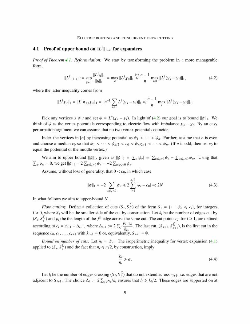
4.1 Proof of upper bound on ‖L†‖1→1 for expanders
Proof of Theorem 4.1. Reformulation: We start by transforming the problem in a more manageableform,
‖L†‖1→1 := supy,0
‖L†y‖1‖y‖1
= maxw‖L†χw‖1
(∗)6
n − 1n
maxs,t‖L†(χs − χt)‖1, (4.2)
where the latter inequality comes from
‖L†χs‖1 = ‖L†π⊥1χs‖1 = ‖n−1∑t,s
L†(χs − χt)‖1 6n − 1
nmax
t‖L†(χs − χt)‖1.
Pick any vertices s , t and set ψ = L†(χs − χt). In light of (4.2) our goal is to bound ‖ψ‖1. Wethink of ψ as the vertex potentials corresponding to electric flow with imbalance χs − χt. By an easyperturbation argument we can assume that no two vertex potentials coincide.
Index the vertices in [n] by increasing potential as ψ1 < · · · < ψn. Further, assume that n is evenand choose a median c0 so that ψ1 < · · · < ψn/2 < c0 < ψn/2+1 < · · · < ψn. (If n is odd, then set c0 toequal the pottential of the middle vertex.)
We aim to upper bound ‖ψ‖1, given as ‖ψ‖1 =∑v |ψv| =
∑v:ψv>0 ψv −
∑u:ψu<0 ψu. Using that∑
w ψw = 0, we get ‖ψ‖1 = 2∑v:ψv>0 ψv = −2
∑u:ψu<0 ψu.
Assume, without loss of generality, that 0 < c0, in which case
‖ψ‖1 = −2∑
u:ψu<0
ψu 6 2n/2∑i=1
|ψi − c0| =: 2N (4.3)
In what follows we aim to upper-bound N.
Flow cutting: Define a collection of cuts (S i, Si ) of the form S i = v : ψv 6 ci, for integers
i > 0, where S i will be the smaller side of the cut by construction. Let ki be the number of edges cut by(S i, S
i ) and pi j be the length of the jth edge across the same cut. The cut points ci, for i > 1, are defined
according to ci = ci−1 − ∆i−1, where ∆i−1 := 2∑
jpi−1, j
ki−1. The last cut, (S r+1, S
r+1), is the first cut in the
sequence c0, c1, . . . , cr+1 with kr+1 = 0 or, equivalently, S r+1 = ∅.
Bound on number of cuts: Let ni = |S i|. The isoperimetric inequality for vertex expansion (4.1)applied to (S i, S
i ) and the fact that ni 6 n/2, by construction, imply
ki
ni> α. (4.4)
Let li be the number of edges crossing (S i, Si ) that do not extend across ci+1, i.e. edges that are not
adjacent to S i+1. The choice ∆i := 2∑
j pi j/ki ensures that li > ki/2. These edges are supported on at
9

JONATHAN KELNER AND PETAR MAYMOUNKOV
least li/dmax vertices in S i, and therefore ni+1 6 ni − li/dmax. Thus,
ni+1 6 ni −li
dmax6 ni −
ki
2dmax
(4.4)6 ni −
αni
2dmax= ni
(1 −
α
2dmax
), (4.5)
Combining inequality (4.5) with n0 = n/2, we get
ni 6n2
(1 −
α
2dmax
)i(4.6)
The stopping condition implies S r , ∅, or nr > 1, and together with (4.6) this results in
r 6 log1/θn2, with θ = 1 −
α
2dmax. (4.7)
Amortization argument: Continuing from (4.3),
N =
n/2∑i=1
|ψi − c0|(∗)6
r∑i=0
(ni − ni+1)i∑
j=0
∆ j, (4.8)
where (∗) follows from the fact that for every vertex v ∈ S i − S i+1 we can write |ψv − c0| 6∑i
j=0 ∆ j.
Because BL†(χs − χt) is a unit flow, we have the crucial (and easy to verify) property that, for all i,∑j pi j = 1. In other words, the total flow of “simulatenous” edges is 1. So,
∆i = 2∑
j
pi j
ki=
2ki
(4.4)6
2αni
(4.9)
Now we can use this bound on ∆ j in (4.8),
r∑i=0
(ni − ni+1)i∑
j=0
∆ j(∗)=
r∑i=1
ni∆i 62α
r∑i=0
1 =2α
(r + 1),
where to derive (∗) we use nr+1 = 0. Combining the above inequality with (4.7) concludes the proof. z
5 Electric walk
To every unit flow f ∈ RE , not necessarily electric, we associate a random walk W = W0,W1, . . . calledthe flow walk, defined as follows. Let σ := B∗ f and so
∑v σv = 0. The walk starts at W0, with
PW0 = v =2 ·max0, σv∑
w |σw|=
∑w fv→w −
∑w fw→v∑
u(∑
w fu→w −∑w fw→u
)10
ELECTRIC ROUTING AND CONCURRENT FLOW CUTTING
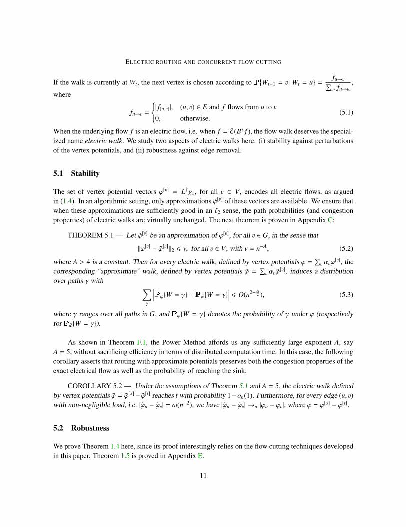
If the walk is currently at Wt, the next vertex is chosen according to PWt+1 = v |Wt = u
=
fu→v∑w fu→w
,
where
fu→v =
| f(u,v)|, (u, v) ∈ E and f flows from u to v
0, otherwise.(5.1)
When the underlying flow f is an electric flow, i.e. when f = E(B∗ f ), the flow walk deserves the special-ized name electric walk. We study two aspects of electric walks here: (i) stability against perturbationsof the vertex potentials, and (ii) robustness against edge removal.
5.1 Stability
The set of vertex potential vectors ϕ[v] = L†χv, for all v ∈ V , encodes all electric flows, as arguedin (1.4). In an algorithmic setting, only approximations ϕ[v] of these vectors are available. We ensure thatwhen these approximations are sufficiently good in an `2 sense, the path probabilities (and congestionproperties) of electric walks are virtually unchanged. The next theorem is proven in Appendix C:
THEOREM 5.1 — Let ϕ[v] be an approximation of ϕ[v], for all v ∈ G, in the sense that
‖ϕ[v] − ϕ[v]‖2 6 ν, for all v ∈ V , with ν = n−A, (5.2)
where A > 4 is a constant. Then for every electric walk, defined by vertex potentials ϕ =∑v αvϕ
[v], thecorresponding “approximate” walk, defined by vertex potentials ϕ =
∑v αvϕ
[v], induces a distributionover paths γ with ∑
γ
∣∣∣∣PϕW = γ −PϕW = γ∣∣∣∣ 6 O(n2− A
2 ), (5.3)
where γ ranges over all paths in G, and PϕW = γ denotes the probability of γ under ϕ (respectivelyfor PϕW = γ).
As shown in Theorem F.1, the Power Method affords us any sufficiently large exponent A, sayA = 5, without sacrificing efficiency in terms of distributed computation time. In this case, the followingcorollary asserts that routing with approximate potentials preserves both the congestion properties of theexact electrical flow as well as the probability of reaching the sink.
COROLLARY 5.2 — Under the assumptions of Theorem 5.1 and A = 5, the electric walk definedby vertex potentials ϕ = ϕ[s]− ϕ[t] reaches t with probability 1−on(1). Furthermore, for every edge (u, v)with non-negligible load, i.e. |ϕu − ϕv| = ω(n−2), we have |ϕu − ϕv| →n |ϕu − ϕv|, where ϕ = ϕ[s] − ϕ[t].
5.2 Robustness
We prove Theorem 1.4 here, since its proof interestingly relies on the flow cutting techniques developedin this paper. Theorem 1.5 is proved in Appendix E.
11
JONATHAN KELNER AND PETAR MAYMOUNKOV
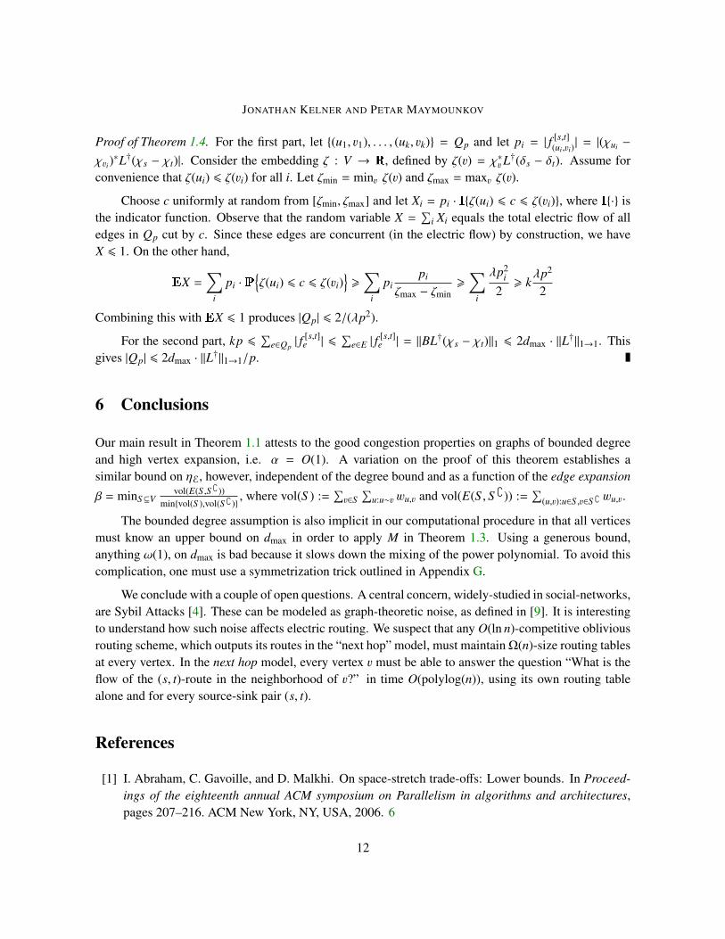
Proof of Theorem 1.4. For the first part, let (u1, v1), . . . , (uk, vk) = Qp and let pi = | f [s,t](ui,vi)| = |(χui −
χvi)∗L†(χs − χt)|. Consider the embedding ζ : V → R, defined by ζ(v) = χ∗vL
†(δs − δt). Assume forconvenience that ζ(ui) 6 ζ(vi) for all i. Let ζmin = minv ζ(v) and ζmax = maxv ζ(v).
Choose c uniformly at random from [ζmin, ζmax] and let Xi = pi · Iζ(ui) 6 c 6 ζ(vi), where I· isthe indicator function. Observe that the random variable X =
∑i Xi equals the total electric flow of all
edges in Qp cut by c. Since these edges are concurrent (in the electric flow) by construction, we haveX 6 1. On the other hand,
EX =∑
i
pi ·Pζ(ui) 6 c 6 ζ(vi)
>
∑i
pipi
ζmax − ζmin>
∑i
λp2i
2> k
λp2
2
Combining this with EX 6 1 produces |Qp| 6 2/(λp2).
For the second part, kp 6∑
e∈Qp | f[s,t]e | 6
∑e∈E | f
[s,t]e | = ‖BL†(χs − χt)‖1 6 2dmax · ‖L†‖1→1. This
gives |Qp| 6 2dmax · ‖L†‖1→1/p. z
6 Conclusions
Our main result in Theorem 1.1 attests to the good congestion properties on graphs of bounded degreeand high vertex expansion, i.e. α = O(1). A variation on the proof of this theorem establishes asimilar bound on ηE, however, independent of the degree bound and as a function of the edge expansion
β = minS⊆Vvol(E(S ,S))
minvol(S ),vol(S), where vol(S ) :=
∑v∈S
∑u:u∼v wu,v and vol(E(S , S )) :=
∑(u,v):u∈S ,v∈S wu,v.
The bounded degree assumption is also implicit in our computational procedure in that all verticesmust know an upper bound on dmax in order to apply M in Theorem 1.3. Using a generous bound,anything ω(1), on dmax is bad because it slows down the mixing of the power polynomial. To avoid thiscomplication, one must use a symmetrization trick outlined in Appendix G.
We conclude with a couple of open questions. A central concern, widely-studied in social-networks,are Sybil Attacks [4]. These can be modeled as graph-theoretic noise, as defined in [9]. It is interestingto understand how such noise affects electric routing. We suspect that any O(ln n)-competitive obliviousrouting scheme, which outputs its routes in the “next hop” model, must maintain Ω(n)-size routing tablesat every vertex. In the next hop model, every vertex v must be able to answer the question “What is theflow of the (s, t)-route in the neighborhood of v?” in time O(polylog(n)), using its own routing tablealone and for every source-sink pair (s, t).
References
[1] I. Abraham, C. Gavoille, and D. Malkhi. On space-stretch trade-offs: Lower bounds. In Proceed-ings of the eighteenth annual ACM symposium on Parallelism in algorithms and architectures,pages 207–216. ACM New York, NY, USA, 2006. 6
12

ELECTRIC ROUTING AND CONCURRENT FLOW CUTTING
[2] I. Abraham, C. Gavoille, D. Malkhi, N. Nisan, and M. Thorup. Compact name-independent routingwith minimum stretch. 2008. 6
[3] F.R.K. Chung. Spectral graph theory. American Mathematical Society, 1997. 6, 20
[4] J.R. Douceur. The sybil attack. In Peer-To-Peer Systems: First International Workshop, Iptps 2002,Cambridge, Ma, USA, March 7-8, 2002, Revised Papers, page 251. Springer, 2002. 12
[5] P.G. Doyle and J.L. Snell. Random walks and electric networks. Arxiv preprint math.PR/0001057,2000. 3
[6] N. Goyal, L. Rademacher, and S. Vempala. Expanders via random spanning trees. In Proceedingsof the Nineteenth Annual ACM-SIAM Symposium on Discrete Algorithms, pages 576–585. Societyfor Industrial and Applied Mathematics Philadelphia, PA, USA, 2009. 6
[7] M.T. Hajiaghayi, R.D. Kleinberg, T. Leighton, and H. Racke. New lower bounds for obliviousrouting in undirected graphs. In Proceedings of the seventeenth annual ACM-SIAM symposium onDiscrete algorithm, pages 918–927. ACM New York, NY, USA, 2006. 3, 8
[8] P. Harsha, T.P. Hayes, H. Narayanan, H. Racke, and J. Radhakrishnan. Minimizing average latencyin oblivious routing. In Proceedings of the nineteenth annual ACM-SIAM symposium on Discretealgorithms, pages 200–207. Society for Industrial and Applied Mathematics Philadelphia, PA,USA, 2008. 6
[9] S. Kale, Y. Peres, and C. Seshadhri. Noise Tolerance of Expanders and Sublinear Expander Recon-struction. In Proceedings of the 2008 49th Annual IEEE Symposium on Foundations of ComputerScience-Volume 00, pages 719–728. IEEE Computer Society Washington, DC, USA, 2008. 12
[10] G. Lawler and H. Narayanan. Mixing times and lp bounds for Oblivious routing. In Workshop onAnalytic Algorithmics and Combinatorics,(ANALCO09). 6
[11] T. Leighton and S. Rao. Multicommodity max-flow min-cut theorems and their use in designingapproximation algorithms. Journal of the ACM (JACM), 46(6):787–832, 1999. 19
[12] H. Racke. Optimal hierarchical decompositions for congestion minimization in networks. InProceedings of the 40th annual ACM symposium on Theory of computing, pages 255–264. ACMNew York, NY, USA, 2008. 6
[13] D.A. Spielman. Graphs and networks, Lecture Notes. 3
[14] D.A. Spielman and N. Srivastava. Graph sparsification by effective resistances. In Proceedings ofthe 40th annual ACM symposium on Theory of computing, pages 563–568. ACM New York, NY,USA, 2008. 14
13

JONATHAN KELNER AND PETAR MAYMOUNKOV
[15] M. Thorup and U. Zwick. Compact routing schemes. In Proceedings of the thirteenth annualACM symposium on Parallel algorithms and architectures, pages 1–10. ACM New York, NY,USA, 2001. 6
[16] M. Thorup and U. Zwick. Approximate distance oracles. Journal of the ACM (JACM), 52(1):1–24,2005. 6
A Proof of Theorem 1.2
Proof of Theorem 1.2. The upper bound follows from:
η(3.1)6 ‖Π‖1→1
(A.2)6 m1/2 · ‖Π‖2→2
(A.3)= m1/2 (A.1)
The second step is justified as follows
‖Π‖1→1 = maxe‖Πχe‖1 6 m1/2 ·max
e‖Πχe‖2 6 m1/2 · ‖Π‖2→2. (A.2)
The third step is the assertion
‖Π‖2→2 6 1, (A.3)
which follows from the (easy) fact that Π is a projection, shown by Spielman, et al. in Lemma A.1.
The lower bound is achieved by a graph obtained by gluing the endpoints of√
n copies of a pathof length
√n and a single edge. Routing a flow of value
√n between these endpoints incurs congestion
√n/2. z
LEMMA A.1 (Proven in [14]) — Π is a projection; Im(Π) = Im(W1/2B); The eigenvalues of Π
are 1 with multiplicity n − 1 and 0 with multiplicity m − n + 1; and Πe,e = ‖Πχe‖2.
B Proof of Theorem 4.2
Proof of Theorem 4.2. Let s , t be a pair of vertices in G at distance D. We consider the flow f =
BL†(χs − χt). Set ψ = L†(χs − χt), and note that we can use ‖ f ‖1 as a lower bound on ‖L†‖1→1,
‖ f ‖1 =∑(u,v)
|ψu − ψv| 6 dmax
∑v
|ψv| 6 dmax‖L†(χs − χt)‖1 6dmax
2‖L†‖1→1.
Now, let πii be a path decomposition of f and let l(πi) and f (πi) denote the length and value, respec-tively, of πi. Then,
‖ f ‖1 =∑(u,v)
|ψu − ψv| =∑
i
l(πi) f (πi) > D∑
i
f (πi) = D. z
14
ELECTRIC ROUTING AND CONCURRENT FLOW CUTTING
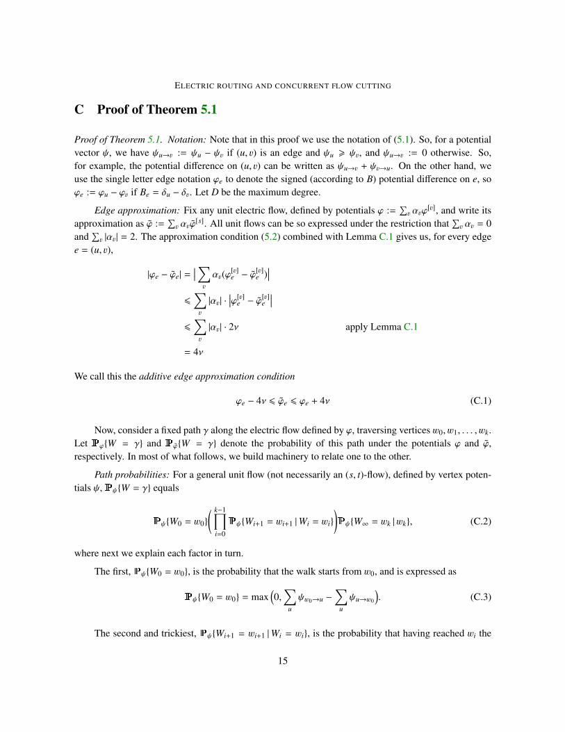
C Proof of Theorem 5.1
Proof of Theorem 5.1. Notation: Note that in this proof we use the notation of (5.1). So, for a potentialvector ψ, we have ψu→v := ψu − ψv if (u, v) is an edge and ψu > ψv, and ψu→v := 0 otherwise. So,for example, the potential difference on (u, v) can be written as ψu→v + ψv→u. On the other hand, weuse the single letter edge notation ϕe to denote the signed (according to B) potential difference on e, soϕe := ϕu − ϕv if Be = δu − δv. Let D be the maximum degree.
Edge approximation: Fix any unit electric flow, defined by potentials ϕ :=∑v αvϕ
[v], and write itsapproximation as ϕ :=
∑v αvϕ
[s]. All unit flows can be so expressed under the restriction that∑v αv = 0
and∑v |αv| = 2. The approximation condition (5.2) combined with Lemma C.1 gives us, for every edge
e = (u, v),
|ϕe − ϕe| =∣∣∣∑
v
αv(ϕ[v]e − ϕ
[v]e )
∣∣∣6
∑v
|αv| ·∣∣∣ϕ[v]
e − ϕ[v]e
∣∣∣6
∑v
|αv| · 2ν apply Lemma C.1
= 4ν
We call this the additive edge approximation condition
ϕe − 4ν 6 ϕe 6 ϕe + 4ν (C.1)
Now, consider a fixed path γ along the electric flow defined by ϕ, traversing vertices w0, w1, . . . , wk.Let PϕW = γ and PϕW = γ denote the probability of this path under the potentials ϕ and ϕ,respectively. In most of what follows, we build machinery to relate one to the other.
Path probabilities: For a general unit flow (not necessarily an (s, t)-flow), defined by vertex poten-tials ψ, PψW = γ equals
PψW0 = w0
( k−1∏i=0
PψWi+1 = wi+1 |Wi = wi
)PψW∞ = wk |wk, (C.2)
where next we explain each factor in turn.
The first, PψW0 = w0, is the probability that the walk starts from w0, and is expressed as
PψW0 = w0 = max(0,
∑u
ψw0→u −∑
u
ψu→w0
). (C.3)
The second and trickiest, PψWi+1 = wi+1 |Wi = wi, is the probability that having reached wi the
15
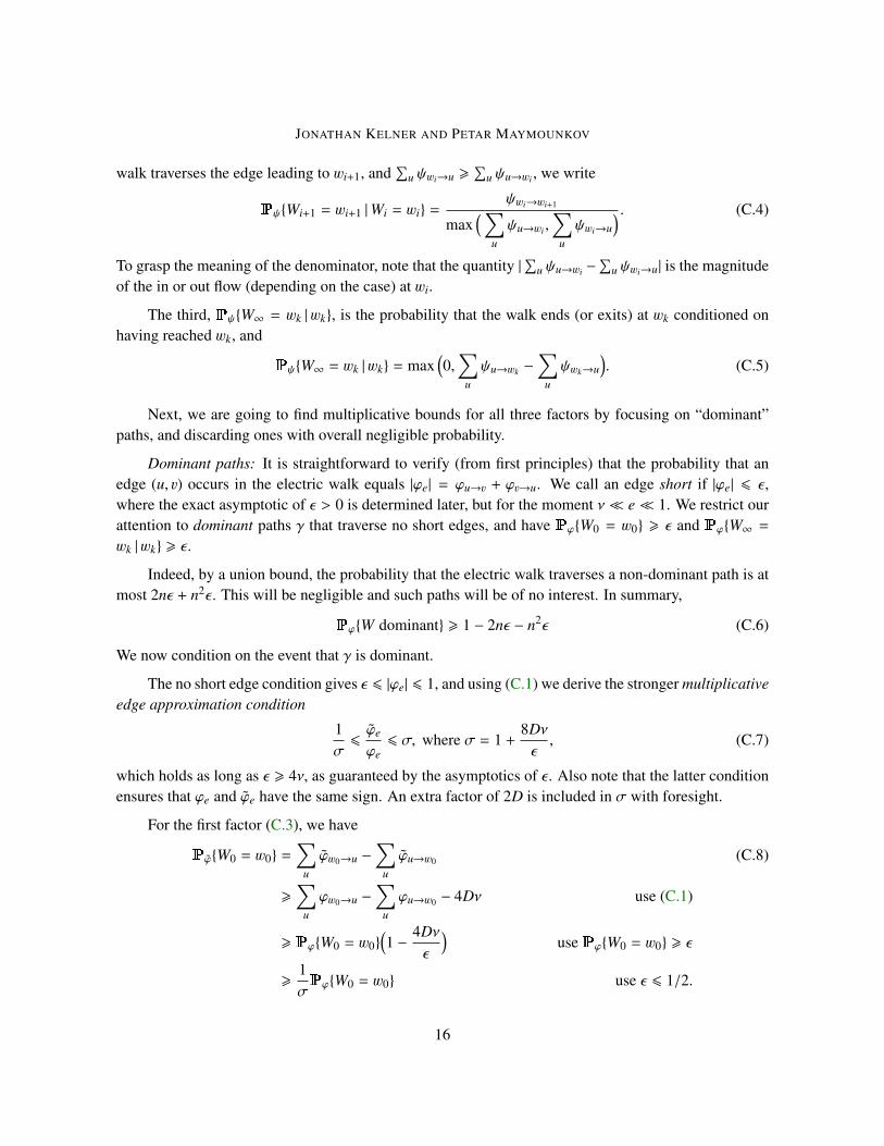
JONATHAN KELNER AND PETAR MAYMOUNKOV
walk traverses the edge leading to wi+1, and∑
u ψwi→u >∑
u ψu→wi , we write
PψWi+1 = wi+1 |Wi = wi =ψwi→wi+1
max(∑
u
ψu→wi ,∑
u
ψwi→u) . (C.4)
To grasp the meaning of the denominator, note that the quantity |∑
u ψu→wi −∑
u ψwi→u| is the magnitudeof the in or out flow (depending on the case) at wi.
The third, PψW∞ = wk |wk, is the probability that the walk ends (or exits) at wk conditioned onhaving reached wk, and
PψW∞ = wk |wk = max(0,
∑u
ψu→wk −∑
u
ψwk→u). (C.5)
Next, we are going to find multiplicative bounds for all three factors by focusing on “dominant”paths, and discarding ones with overall negligible probability.
Dominant paths: It is straightforward to verify (from first principles) that the probability that anedge (u, v) occurs in the electric walk equals |ϕe| = ϕu→v + ϕv→u. We call an edge short if |ϕe| 6 ε,where the exact asymptotic of ε > 0 is determined later, but for the moment ν e 1. We restrict ourattention to dominant paths γ that traverse no short edges, and have PϕW0 = w0 > ε and PϕW∞ =
wk |wk > ε.
Indeed, by a union bound, the probability that the electric walk traverses a non-dominant path is atmost 2nε + n2ε. This will be negligible and such paths will be of no interest. In summary,
PϕW dominant > 1 − 2nε − n2ε (C.6)
We now condition on the event that γ is dominant.
The no short edge condition gives ε 6 |ϕe| 6 1, and using (C.1) we derive the stronger multiplicativeedge approximation condition
1σ6ϕe
ϕe6 σ, where σ = 1 +
8Dνε, (C.7)
which holds as long as ε > 4ν, as guaranteed by the asymptotics of ε. Also note that the latter conditionensures that ϕe and ϕe have the same sign. An extra factor of 2D is included in σ with foresight.
For the first factor (C.3), we have
PϕW0 = w0 =∑
u
ϕw0→u −∑
u
ϕu→w0 (C.8)
>∑
u
ϕw0→u −∑
u
ϕu→w0 − 4Dν use (C.1)
> PϕW0 = w0(1 −
4Dνε
)use PϕW0 = w0 > ε
>1σPϕW0 = w0 use ε 6 1/2.
16

ELECTRIC ROUTING AND CONCURRENT FLOW CUTTING
For the second factor (C.4), assume∑
u ψu→wi >∑
u ψwi→u. An identical argument holds in theother case. Abbreviate
Pϕwi+1 |wi := PϕWi+1 = wi+1 |Wi = wi.
Path dominance implies∑
u ϕu→wi > ε, and so
Pϕwi+1 |wi =ϕwi→wi+1∑u
ϕu→wi
(C.9)
>σ−1 · ϕwi→wi+1∑u
ϕu→wi + 4Dνuse (C.7) and (C.1)
> σ−2 ϕwi→wi+1∑u ϕu→wi
use ε 6 1/2 and∑
u
ϕu→wi > ε
=1σ2Pϕwi+1 |wi.
For the third factor (C.5), similarly to the first, we have
PϕW∞ = wk |wk = (C.10)
=∑
u
ϕu→wk −∑
u
ϕwk→u
>∑
u
ϕu→wk −∑
u
ϕwk→u − 4Dν use (C.1)
> PϕW∞ = wk |wk(1 −
4Dνε
)use PϕW∞ = wk |wk > ε
>1σPϕW∞ = wk |wk use ε 6 1/2.
Dominant path bound: We now obtain a relation between PϕW = γ andPϕW = γ by combing-ing the bounds (C.8), (C.9) and (C.10) with (C.2):
PϕW = γ
PϕW = γ>
1σ2n+2 apply bounds, and path length 6 n (C.11)
>(1 −
8Dνε
)2n+2use σ−1 > 1 − 8Dν/ε
> exp(−
16Dνε
)2n+2use 1 − x > e−2x
=: θ
Statistical difference: Abbreviate p(γ) := PϕW = γ and q(γ) := PϕW = γ. Below, γ iteratesthrough all paths, ζ iterates through dominant paths and ξ iterates through non-dominant paths. We
17
JONATHAN KELNER AND PETAR MAYMOUNKOV
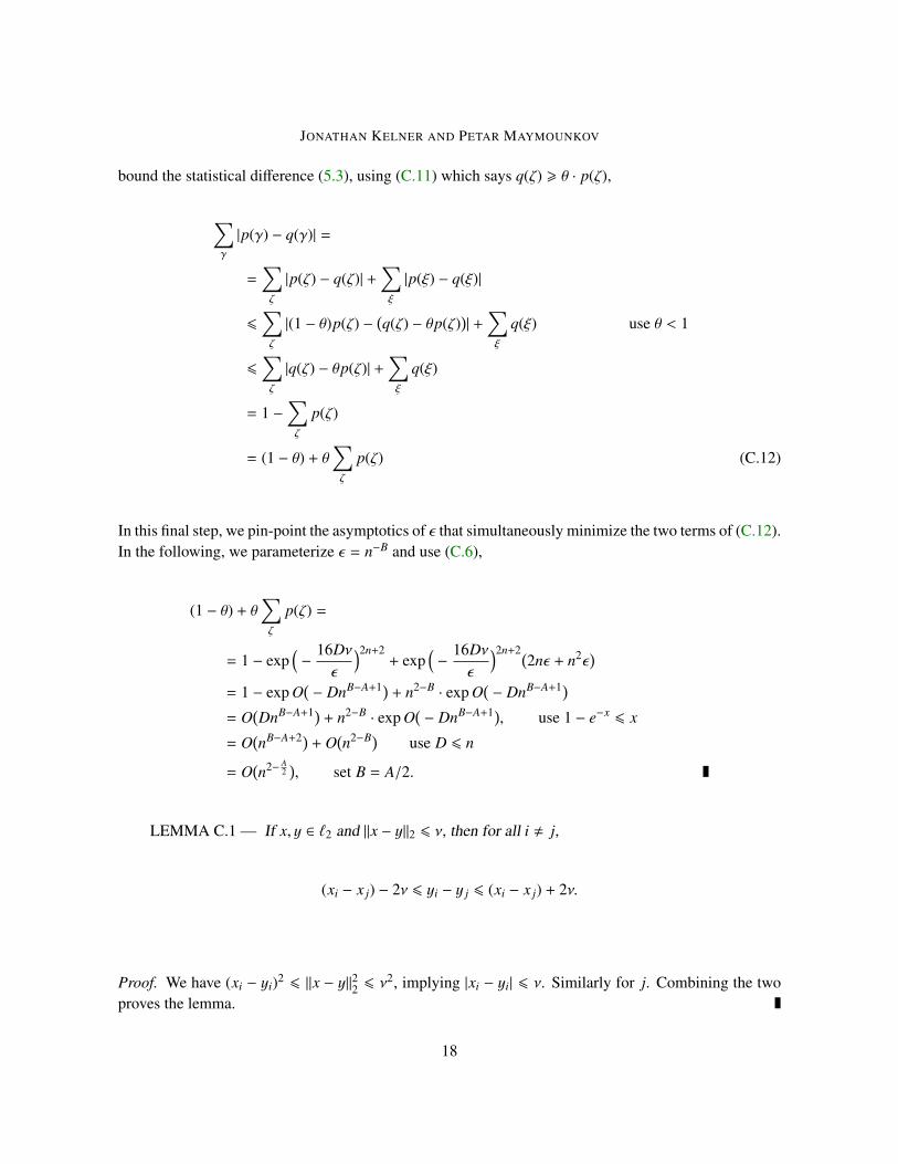
bound the statistical difference (5.3), using (C.11) which says q(ζ) > θ · p(ζ),
∑γ
|p(γ) − q(γ)| =
=∑ζ
|p(ζ) − q(ζ)| +∑ξ
|p(ξ) − q(ξ)|
6∑ζ
|(1 − θ)p(ζ) −(q(ζ) − θp(ζ)
)| +
∑ξ
q(ξ) use θ < 1
6∑ζ
|q(ζ) − θp(ζ)| +∑ξ
q(ξ)
= 1 −∑ζ
p(ζ)
= (1 − θ) + θ∑ζ
p(ζ) (C.12)
In this final step, we pin-point the asymptotics of ε that simultaneously minimize the two terms of (C.12).In the following, we parameterize ε = n−B and use (C.6),
(1 − θ) + θ∑ζ
p(ζ) =
= 1 − exp(−
16Dνε
)2n+2+ exp
(−
16Dνε
)2n+2(2nε + n2ε
)= 1 − exp O
(− DnB−A+1) + n2−B · exp O
(− DnB−A+1)
= O(DnB−A+1) + n2−B · exp O
(− DnB−A+1), use 1 − e−x 6 x
= O(nB−A+2) + O
(n2−B) use D 6 n
= O(n2− A
2), set B = A/2. z
LEMMA C.1 — If x, y ∈ `2 and ‖x − y‖2 6 ν, then for all i , j,
(xi − x j) − 2ν 6 yi − y j 6 (xi − x j) + 2ν.
Proof. We have (xi − yi)2 6 ‖x − y‖22 6 ν2, implying |xi − yi| 6 ν. Similarly for j. Combining the two
proves the lemma. z
18

ELECTRIC ROUTING AND CONCURRENT FLOW CUTTING
D Proof of Theorem 1.6
Proof of Theorem 1.6. Let X[s,t]e be the indicator that edge e participates in the electric walk between s
and t. Then the latency can be expressed as
maxs,t
∑e
EX[s,t]e = max
s,t
∑(u,v)
∣∣∣(δu − δv)L†(δs − δt)∣∣∣
= maxs,t‖BL†(δs − δt)‖1 = ‖BL†B∗‖1→1 = ‖Π‖1→1.
The latter is bounded by Theorem 4.1 and ‖Π‖1→1 6 m1/2, as in (A.1) e.g. z
Remark D.1 — For expanders, this theorem is not trivial. In fact, there exist path realizations ofthe electric walk which can traverse up to O(n) edges. Theorem 1.6 asserts that this happens with smallprobability. On the other hand, in a bounded-degree expander, even if s and t are adjacent the walk willstill take a O(log n)-length path with constant probability.
E Proof of Theorem 1.5
Proof of Theorem 1.5. Let fopt be a max-flow routing of the uniform demands and let θ be the fraction ofthe demand set that is routed by fopt. The Multi-commodity Min-cut Max-flow Gap Theorem (Theorem2, in [11]) asserts
O(ln n) · θ > minS⊂V
|E(S , S )|
|S | · |S |>
1n·min
S⊂V
|E(S , S )|
min|S |, |S |=α
n
Thus the total demand flown by fopt is no less than θ(n2
)> Ω(αn/ ln n). Normalize f (by scaling) so it
routes the same demands as fopt. If k edges are removed, then at most ηk flow is removed from f , whichis at most a fraction ηk ·O(ln n/αn) of the total flow. Substitute x = k/m and use m 6 dmaxn to completethe proof. z
F Proof of Theorem 1.3
Theorem 1.3 is implied by the following theorem by specializing ε = O(n−5):
THEOREM F.1 — Let G be a graph, whose Laplacian L has smallest eigenvalue λ and whosemaximum degree is D. Then, for every y with ‖y‖2 = 1 the vector x = L†y can be approximated using
x =1
2D
d∑i=0
(I −
L2D
)iy,
19
JONATHAN KELNER AND PETAR MAYMOUNKOV
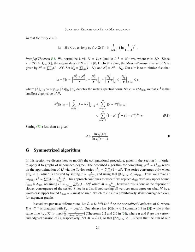
so that for every ε > 0,
‖x − x‖2 6 ε, as long as d > Ω(1) · ln1λεD
·(
ln1
1 − λ
)−1.
Proof of Theorem F.1. We normalize L via N = L/τ (and so L−1 = N−1/τ), where τ = 2D. Sinceτ = 2D > λmax(L), the eigenvalues of N are in [0, 1]. In this case, the Moore-Penrose inverse of N isgiven by N† =
∑∞i=0(I − N)i. Set N†0 =
∑di=0(I − N)i and N†1 = N† − N†0 . Our aim is to minimize d so that
‖x − x‖2 =∥∥∥∥N†0 + N†1
τy −
N†0τy∥∥∥∥
2=
∥∥∥∥N†1τy∥∥∥∥
26
∥∥∥∥N†1τ
∥∥∥∥2→26 ε,
where ‖A‖2→2 := supx,0 ‖Ax‖2/‖x‖2 denotes the matrix spectral norm. Set κ := τ/λmin, so that κ−1 is thesmallest eigenvalue of N,
‖N†1‖2→2 =∥∥∥ ∞∑
i=d+1
(I − N)i∥∥∥
2→2 6∞∑
i=d+1
‖(I − N)i‖2→2
6∞∑
i=d+1
(1 − κ−1
)i= (1 − κ−1)d+1κ (F.1)
Setting (F.1) less than τε gives
d >ln κ/(τε)
ln κ/(κ − 1). z
G Symmetrized algorithm
In this section we discuss how to modify the computational procedure, given in the Section 1, in orderto apply it to graphs of unbounded degree. The described algorithm for computing ϕ[w] = L†χw relieson the approximation of L† via the Taylor series 1
1−x =∑∞
i=0(1 − x)i. The series converges only when‖x‖2 < 1, which is ensured by setting x = L
2dmax, and using that ‖L‖2→2 < 2dmax. Thus we arrive at
2dmax · L† =∑∞
i=0(I − L2dmax
)i. This approach continues to work if we replace dmax with any upper boundhmax > dmax, obtaining L† = 1
2hmax
∑∞i=0(I −M)i where M = L
2hmax, however this is done at the expense of
slower convergence of the series. Since in a distributed setting all vertices must agree on what M is, aworst-case upper bound hmax = n must be used, which results in a prohibitively slow convergence evenfor expander graphs.
Instead, we pursue a differnt route. Let L = D−1/2LD−1/2 be the normalized Laplacian of G, whereD ∈ Rn×n is diagonal with Dv,v = deg(v). One always has ‖L‖2→2 6 2 (Lemma 1.7 in [3]) while at thesame time λmin(L) > max
β2
2 ,α2
4dmax+2dmaxα
(Theorems 2.2 and 2.6 in [3]), where α and β are the vertex-
and edge-expansion of G, respectively. Set M = L/3, so that ‖M‖2→2 < 1. Recall that the aim of our
20
ELECTRIC ROUTING AND CONCURRENT FLOW CUTTING
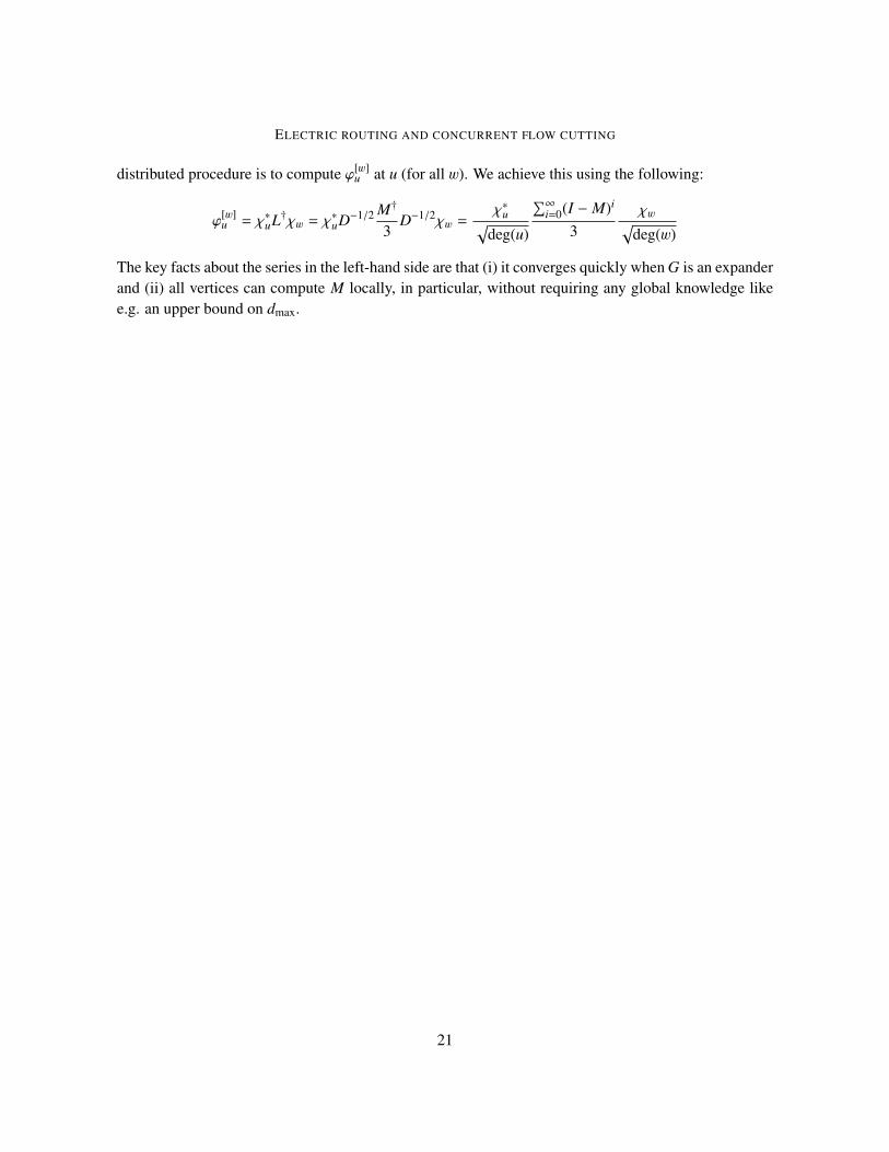
distributed procedure is to compute ϕ[w]u at u (for all w). We achieve this using the following:
ϕ[w]u = χ∗uL†χw = χ∗uD−1/2 M†
3D−1/2χw =
χ∗u√deg(u)
∑∞i=0(I − M)i
3χw√
deg(w)
The key facts about the series in the left-hand side are that (i) it converges quickly when G is an expanderand (ii) all vertices can compute M locally, in particular, without requiring any global knowledge likee.g. an upper bound on dmax.
21