electric potential in plasma and sheath regions with ... · author’s e-mail:...

author’s e-mail: [email protected]

Electric Potential in Plasma and Sheath Regions with Magnetic Field Increasing

toward a Wall

Azusa FUKANO and Akiyoshi HATAYAMA1)

Monozukuri Department, Tokyo Metropolitan College of Industrial Technology, Shinagawa, Tokyo 140-0011 1)

Faculty of Science and Technology, Keio University, Yokohama 223-8522, Japan

Electric potential near a wall in plasma with magnetic field increasing toward a wall is investigated analytically. A

magnetic field that is symmetric about an axis and increases monotonically toward the wall is considered. The potential

profile is analyzed by solving the plasma-sheath equation that gives the electric potential in the plasma region and the

sheath region near the wall self-consistently. The potential in the plasma region depends on the profile of the magnetic field

and the ion temperature. As the magnetic field near the wall increases and the ratio of the ion temperature to the electron

temperature decreases, the potential drop in the plasma region decreases. The potential also depends on a ratio of the

increase rate of the magnetic field to the decrease rate of the potential toward the wall. When the increase rate of the

magnetic field is larger than the decrease rate of the potential, the potential drop in the plasma region becomes large

compared with that in the magnetic field of which increase rate is smaller than the decrease rate of the potential.

Keywords: negative ion source, cusp magnetic field, cusp loss width, heat transmission coefficient, electric potential,

plasma region, sheath region, plasma-sheath equation,

1. Introduction

Neutral beam injection (NBI) using negative ion

source is one of the most promising method of heating

plasma confined magnetically in Tokamak. Plasma in a

negative ion source is confined by a cusp magnetic field in

order to reduce plasma loss on the wall. However, plasma

particles that arrive to the cusp magnetic field move along

the magnetic field and are lost through the cusp magnet

region on the wall. Therefore, in plasma confinement in the

ion source, it is important to investigate the plasma loss

through the cusp magnetic field, especially the width of the

plasma loss region, the so-called ‘cusp loss width’. It has

been indicated that the cusp loss width of electron energy

depends on a heat transmission coefficient defined by the

ratio of the heat flux to the particle flux multiplied by the

electron temperature along the magnetic field [1]. In

general, a sheath potential is formed in the plasma near the

wall surface. Since the heat transmission coefficient is

determined by the sheath potential near the wall [2], the

sheath potential needs to be investigated in plasma

confinement in the ion source.

Emmert et al. investigated formation of the potential

considering both the plasma region and the sheath region

self-consistently by using a plasma-sheath equation [3].

Sato et al. extended the method of Emmert et al. to a case

of magnetized plasma. In their analysis, the magnetic field

of which strength decreases monotonically toward the wall

was considered [4]. However, the potential formation in

the plasma and the sheath regions for the case of the

magnetic field of which strength increases toward the wall

such as the cusp magnetic in the negative ion sources has

not been clearly understood.

In this paper, we will investigate the potential profile

near the wall in plasma with the cusp magnetic field

increasing monotonically toward the wall. The

plasma-sheath equation is derived and solved

self-consistently over the region from the plasma to the wall,

where not only a magnitude of the magnetic field but also a

ratio of the increase rate of the magnetic field to the

decrease rate of the potential toward the wall is considered.

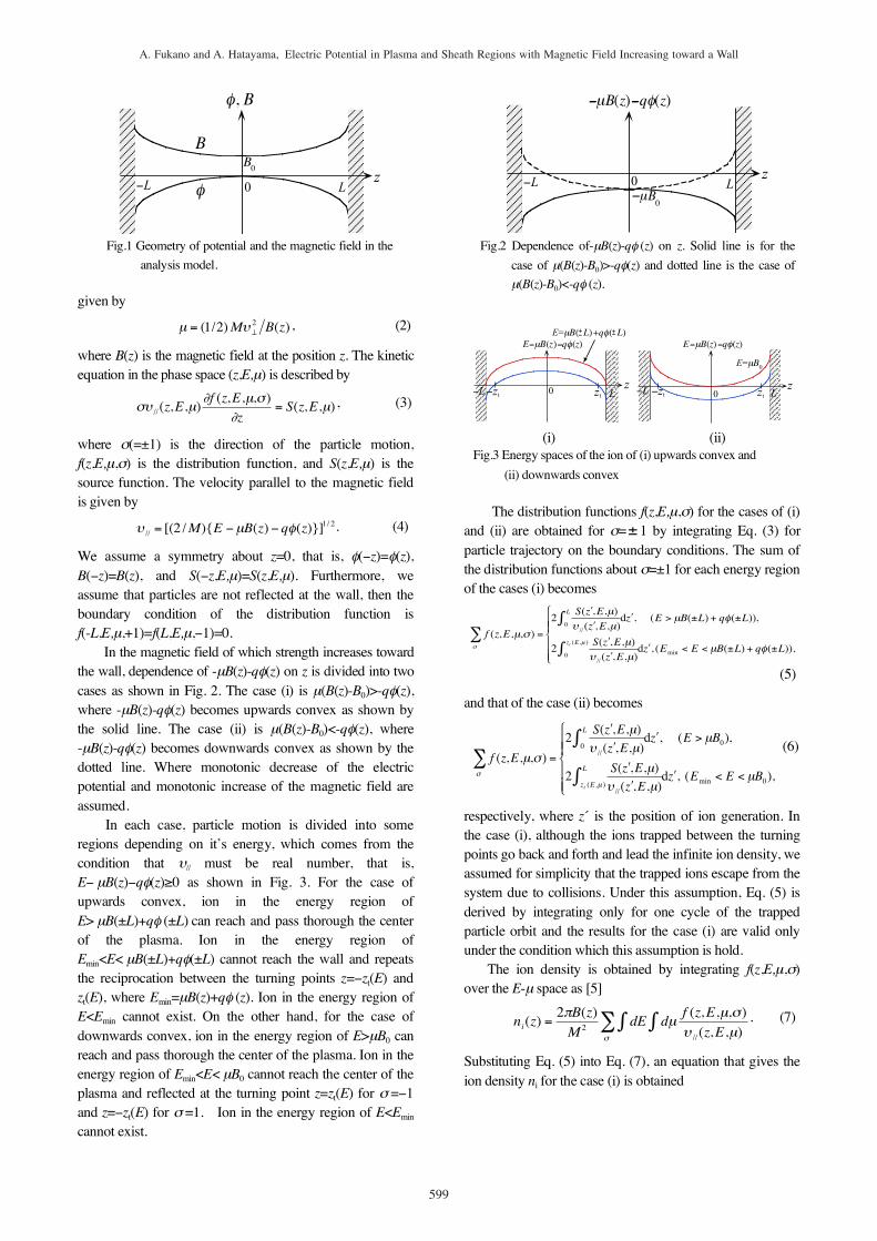
2. Model

The geometry of analytical model is shown in Fig. 1.

The electric potential φ(z) is assumed to be symmetric about

z=0 and decreases monotonically for z>0 and zero at z=0.

The magnetic field is assumed to be symmetric about z=0

and increases monotonically for z>0 and B0 at z=0. Plasma

is assumed to consist of electrons and positive hydrogen

ions.

3. Analysis of Electric Potential

Constant energy E of an ion in the z-direction is

!

E =1

2M("#

2+"

//

2) + q$(z) , (1)

where M is the ion mass, υ⊥ and υ// are the velocities

perpendicular and parallel to the magnetic field, and q is the

charge of the ion, respectively. The magnetic moment is

598

J. Plasma Fusion Res. SERIES, Vol. 9 (2010)

©2010 by The Japan Society of PlasmaScience and Nuclear Fusion Research

(Received: 18 October 2009 / Accepted: 28 March 2010)

given by

!

µ = (1/2)M"#

2B(z) , (2)

where B(z) is the magnetic field at the position z. The kinetic

equation in the phase space (z,E,µ) is described by

!

"#//(z,E,µ)

$f (z,E,µ," )

$z= S(z,E,µ) , (3)

where σ(=±1) is the direction of the particle motion,

f(z,E,µ,σ) is the distribution function, and S(z,E,µ) is the

source function. The velocity parallel to the magnetic field

is given by

!

"//

= [(2 /M){E #µB(z) # q$(z)}]1/ 2. (4)

We assume a symmetry about z=0, that is, φ(−z)=φ(z),

B(−z)=B(z), and S(−z,E,µ)=S(z,E,µ). Furthermore, we

assume that particles are not reflected at the wall, then the

boundary condition of the distribution function is

f(-L,E,µ,+1)=f(L,E,µ,−1)=0.

In the magnetic field of which strength increases toward

the wall, dependence of -µB(z)-qφ(z) on z is divided into two

cases as shown in Fig. 2. The case (i) is µ(B(z)-B0)>-qφ(z),

where -µB(z)-qφ(z) becomes upwards convex as shown by

the solid line. The case (ii) is µ(B(z)-B0)<-qφ(z), where

-µB(z)-qφ(z) becomes downwards convex as shown by the

dotted line. Where monotonic decrease of the electric

potential and monotonic increase of the magnetic field are

assumed.

In each case, particle motion is divided into some

regions depending on it’s energy, which comes from the

condition that υ// must be real number, that is,

E− µB(z)−qφ(z)≥0 as shown in Fig. 3. For the case of

upwards convex, ion in the energy region of

E> µB(±L)+qφ (±L) can reach and pass thorough the center

of the plasma. Ion in the energy region of

Emin<E< µB(±L)+qφ(±L) cannot reach the wall and repeats

the reciprocation between the turning points z=−zt(E) and

zt(E), where Emin=µB(z)+qφ (z). Ion in the energy region of

E<Emin cannot exist. On the other hand, for the case of

downwards convex, ion in the energy region of E>µB0 can

reach and pass thorough the center of the plasma. Ion in the

energy region of Emin<E< µB0 cannot reach the center of the

plasma and reflected at the turning point z=zt(E) for σ =−1

and z=−zt(E) for σ =1. Ion in the energy region of E<Emin

cannot exist.

The distribution functions f(z,E,µ,σ) for the cases of (i)

and (ii) are obtained for σ=

!

± 1 by integrating Eq. (3) for

particle trajectory on the boundary conditions. The sum of

the distribution functions about σ=±1 for each energy region

of the cases (i) becomes

!

f (z,E,µ," )"

# =

2S( $ z ,E,µ)

% // ( $ z ,E,µ)0

L

& d $ z , (E > µB(±L) + q'(±L)),

2S( $ z ,E,µ)

% // ( $ z ,E,µ)0

zt (E ,µ )& d $ z , (Emin < E < µB(±L) + q'(±L)),

(

)

* *

+

* *

(5)

and that of the case (ii) becomes

!

f (z,E,µ," )"

# =

2S( $ z ,E,µ)

% // ( $ z ,E,µ)0

L

& d $ z , (E > µB0),

2S( $ z ,E,µ)

% // ( $ z ,E,µ)zt (E ,µ )

L

& d $ z , (Emin < E < µB0),

'

(

) )

*

) )

(6)

respectively, where z´ is the position of ion generation. In

the case (i), although the ions trapped between the turning

points go back and forth and lead the infinite ion density, we

assumed for simplicity that the trapped ions escape from the

system due to collisions. Under this assumption, Eq. (5) is

derived by integrating only for one cycle of the trapped

particle orbit and the results for the case (i) are valid only

under the condition which this assumption is hold.

The ion density is obtained by integrating f(z,E,µ,σ)

over the E-µ space as [5]

!

ni(z) =2"B(z)

M2

dE dµf (z,E,µ,#)

$//(z,E,µ)

%%#

& . (7)

Substituting Eq. (5) into Eq. (7), an equation that gives the

ion density ni for the case (i) is obtained

z

φ 0 L−L

B

B0

φ, B

Fig.1 Geometry of potential and the magnetic field in the

analysis model.

z0 L−L−µB

0

-µB(z)-qφ(z)

Fig.2 Dependence of-µB(z)-qφ (z) on z. Solid line is for the

case of µ(B(z)-B0)>-qφ(z) and dotted line is the case of

µ(B(z)-B0)<-qφ (z).

z0 L−L

E=µB( L)+qφ( L)- -+ +

zt−zt

E-µB(z)-qφ(z)

z0 L−L

E=µB0

zt−zt

E-µB(z)-qφ(z)

(i) (ii)

Fig.3 Energy spaces of the ion of (i) upwards convex and

(ii) downwards convex

599

A. Fukano and A. Hatayama, Electric Potential in Plasma and Sheath Regions with Magnetic Field Increasing toward a Wall

!

ni(z) =4"B(z)

M2

dE#q$ (z)B(±L )

B(z)#B0+q$ (±L )

%

&'

( )

* dµ1

+//(z,E,µ)

#q$ (z)

B(z)#B0

1

B (±L ){E#q$ (±L )}

&S( , z ,E,µ)

+//( , z ,E,µ)

d , z 0

L

&

+ dE dµ#q$ (z)

B(z)#B0

1

B (z ){E#q$ (z)}

&#q$ (z )B (z )

B(z)#B0+q$ (z )

#q$ (z)B(±L )

B(z)#B0+q$ (±L )

&1

+//(z,E,µ)

*S( , z ,E,µ)

+//( , z ,E,µ)

d , z 0

zt (E ,µ )& + dE#q$ (z )B (±L )

B (z )#B0+q$ (±L )

%

&

* dµ1

+//(z,E,µ)

S( , z ,E,µ)

+//( , z ,E,µ)

d , z 0

zt (E ,µ )&1

B (±L ){E#q$ (±L )}

1

B(z){E#q$ (z )}

&-

. / .

(8)

And substituting Eq. (6) into Eq. (7), that for the case (ii) is

obtained

!

ni(z) =4"B(z)

M2

# dE dµ1

$//(z,E,µ)

S( % z ,E,µ)

$//( % z ,E,µ)

d % z 0

L

&0

E

B0&0

'q( (z )B0B (z )'B0&

)

* +

+ dE dµ1

$//(z,E,µ)

S( % z ,E,µ)

$//( % z ,E,µ)

d % z 0

L

&0

'q( (z)

B(z)'B0&'q( (z )B0B (z )'B0

,

&

+ dE dµ1

$//(z,E,µ)

S( % z ,E,µ)

$//( % z ,E,µ)

d % z zt

L

&E

B0

1

B (z ){E'q( (z)}

&0

'q( (z)B0B(z)'B0&

+ dE dµ1

$//(z,E,µ)

S( % z ,E,µ)

$//( % z ,E,µ)

d % z zt

L

&0

1

B (z ){E'q( (z)}

&q( (z)

0

&-

. / .

(9)

The integral regions of E and µ are divided to two cases

according to the conditions that υ// must be real number for

each case of (i) and (ii). The case (a) is the increase rate of

the magnetic field is smaller than the decrease rate of the

potential, that is, (B(z)-B0)/(B(z’)-B0)<φ(z)/φ (z’) for z’<z and

(B(z)-B0)/(B(z’)-B0)>φ(z)/φ (z’) for z’>z. The case (b) is the

increase rate of the magnetic field is larger than the decrease

rate of the potential, that is, (B(z)-B0)/(B(z’)-B0)>φ(z)/φ (z’)

for z’<z and (B(z)-B0)/(B(z’)-B0)<φ(z)/φ (z’) for z’>z.

By interchanging the order of integrations of Eqs. (8)

and (9) and taking sum of the integrations of them for each

case of (a) and (b), respectively, the ion density can be

written as for the case (a)

!

ni(z) =4"B(z)

M2

d # z 0

L

$ dE%E p B0

B p %B0

&

$'

( ) )

* dµ1

+//(z,E,µ)

S( # z ,E,µ)

+//( # z ,E,µ)0

1

B (z ){E%q, (z)}

$

+ d # z 0

L

$ dE dµ1

+//(z,E,µ)

S( # z ,E,µ)

+//( # z ,E,µ)0

1

B p

(E%E p )$E p

%E p B0

B p %B0$-

. / ,

(10)

and for the case (b)

!

ni(z) =4"B(z)

M2

d # z 0

L

$ dE%Es B0

Bs %B0

&

$'

( )

* dµ1

+//(z,E,µ)

S( # z ,E,µ)

+//( # z ,E,µ)0

1

Bs

(E%Es )$

+ d # z 0

L

$ dE dµ1

+//(z,E,µ)

S( # z ,E,µ)

+//( # z ,E,µ)0

1

B(z){E%q, (z )}

$q, (z )

%Es B0

Bs %B0$-

. / ,

(11)

where Ep=qφ(z’), Bp=B(z’), Es=qφ (z) and Bs=B (z) for z’<z

and Ep=qφ(z), Bp=B(z), Es=qφ (z’) and Bs=B (z’) for z’>z

according to the conditions that υ// must be real number.

As the source function S(z,E,µ), we use the expression

same as Emmert et al. [3]

!

S(z,E,µ) = S0h(z)M

2

4" (kTi)2# // (z,E,µ)exp $

E $ e%(z)

kTi

& ' (

) * +

, (12)

where Ti is the temperatures, h(z) is the source strength, and

S0 is the average source strength of the ion, respectively.

Substituting Eq. (12) into Eqs. (10) and (11) and integrating

them for µ and E, the ion density becomes

!

ni(z) = S

0

"M

2kTi

#

$ %

&

' (

1/ 2

d ) z 0

L

* I(z, ) z )h( ) z ) , (13)

where I(z, z’) is given by

case (a):

!

I(z,z') =

expq"( # z ) $ q"(z)

kTi

% & '

( ) * erfc

q"( # z ) $ q"(z)

kTi

% & '

( ) *

1/ 2+

, - -

.

/ 0 0

+2

1

(B(z) $ B0)q"( # z ) $ (B( # z ) $ B0)q"(z)

kTi(B( # z ) $ B0)

% & '

( ) *

1/ 2

2 expq"( # z )B( # z )

kTi(B( # z ) $ B0)

% & '

( ) *

+B(z) $ B( # z )

B( # z )

% & '

( ) *

1/ 22

1

2 exp(q"( # z ) $ q"(z))B( # z )

kTi(B( # z ) $ B(z))

% & '

( ) *

D $(q"( # z ) $ q"(z))B( # z )

kTi(B( # z ) $ B(z))

% & '

( ) *

1/ 2+

, - -

.

/ 0 0

+

,

- -

$D $(B(z) $ B0)q"( # z ) $ (B( # z ) $ B0)q"(z){ }B( # z )

kTi(B( # z ) $ B(z))(B( # z ) $ B0)

% & '

( ) *

1/ 2+

, - -

.

/ 0 0

.

/

0 0 , # z < z,

expq"( # z ) $ q"(z)

kTi

% & '

( ) * , # z > z ,

%

&

3 3 3 3 3 3 3 3 3 3

'

3 3 3 3 3 3 3 3 3 3

(14)

case (b):

!

I(z,z') =

expq"( # z ) $ q"(z)

kTi

% & '

( ) *

erfcq"( # z ) $ q"(z)

kTi

% & '

( ) *

1/ 2+

, - -

.

/ 0 0 , # z < z ,

expq"( # z ) $ q"(z)

kTi

% & '

( ) * $

2

1

(B(z) $ B0)q"( # z )

kTi(B( # z ) $ B0)$

q"(z)

kTi

% & '

( ) *

1/ 2

2 expB( # z )q"( # z )

kTi(B( # z ) $ B0)

% & '

( ) * $

B( # z ) $ B(z)

B( # z )

% & '

( ) *

1/ 2

2 erfcB( # z )

B( # z ) $ B(z)

(B(z) $ B0)q"( # z )

kTi(B( # z ) $ B0)$

q"(z)

kTi

% & '

( ) *

% & '

( ) *

+

, - -

.

/ 0 0

, # z > z ,

%

&

3 3 3 3 3 3

'

3 3 3 3 3 3

(15)

Where D(z) is the Dawson function [5]

!

D(x) = exp(t2)dt

0

x

" . (16)

For the electron density ne, we use a Maxwell−Boltzmann

600


distribution for simplicity

!

ne(z) = n0 exp{e"(z) /kTe}, (17)

where n0 is the density at z=0, −e is the electron charge, k is

the Boltzmann’s constant, and Te is the electron temperature.

Substituting Eqs. (13) and (17) into Poisson’s equation,

the plasma-sheath equation is derived as

!

"D

2 e

kTe

d2#

dz2

= expe#(z)

kTe

$

% &

'

( ) *

q

e

S0

n0

+M

2kTi

$

% &

'

( )

1/ 2

d , z 0

L

- I(z, , z )h( , z ) ,

(18)

where λD=(ε0kTe/n0e2)1/2 is the Debye length. The average

source strength S0 is decided by the equilibrium of the fluxes

of the plasma particles at the wall. We consider that

jiw+jew=0, where jiw is the ion current density and jew is the

electron current density at the wall, then

!

S0q

eL = n0

kTe

2"m

#

$ %

&

' (

1/ 2

expe)wkTe

#

$ %

&

' ( , (19)

where m is the electron mass and φw is the wall potential.

Substituting S0 given by Eq. (19) into Eq. (18), we obtain

!

"D

2 e

kTe

d2#(z)

dz2

= expe#(z)

kTe

$

% &

'

( ) *

1

2L

M

m

Te

Ti

$

% &

'

( )

1/ 2

expe#

w

kTe

$

% &

'

( )

+ d , z 0

L

- I(z, , z )h( , z ). (20)

4. Numerical Solution of the Plasma-Sheath

Equation

Here, we introduce the normalized variables:

η=(e/kTe)(φw−φ), s=z/L, τ=Te/Ti, Z=q/e, R=B/B0, where R is

the mirror ratio. Equation (20) is normalized as

!

A2 d

2"

ds2

=1

2

M

m#

$

% &

'

( )

1/ 2

d * s 0

1

+ I(", * " )h( * s ) , exp(,"), (21)

where η=η(s), η'=η(s'), A2=(λD2/L2)exp(−eφw/kTe), and

I(η,η’) is given by

case (a):

!

I(", # " ) =

exp Z$(" % # " ){ }erfc Z$(" % # " ){ }1/ 2[ ]

+2

&

R(") %1

R( # " ) %1

q'wkTi

% Z$ # " (

) *

+

, - %

q'wkTi

% Z$"(

) *

+

, -

. / 0

1 2 3

1/ 2

4 expR( # " )

R( # " ) %1

q'wkTi

% Z$ # " (

) *

+

, -

. / 0

1 2 3

+R(") % R( # " )

R( # " )

. / 0

1 2 3

1/ 2

2

&

4 expR( # " )

R( # " ) % R(")Z$(" % # " )

. / 0

1 2 3 D

%R( # " )

R( # " ) % R(")Z$(" % # " )

. / 0

1 2 3

1/ 25

6 7 7

8

9 : :

5

6

7 7

%D %R( # " )

R( # " ) % R(")

R(") %1

R( # " ) %1

q'wkTi

% Z$ # " (

) *

+

, -

. / 0

. / ;

0 ;

5

6 7 7

%q'wkTi

% Z$"(

) *

+

, - 1 2 3

1 2 ;

3 ;

1/ 28

9

: :

8

9

: : , # " <" ,

exp Z$(" % # " ){ } , # " >" ,

.

/

; ; ; ; ; ; ; ; ; ;

0

; ; ; ; ; ; ; ; ; ;

(22)

case (b):

!

I(", # " ) =

exp Z$(" % # " ){ }erfc Z$(" % # " ){ }1/ 2[ ] , # " <" ,

exp Z$(" % # " ){ }%2

&

R(") %1

R( # " ) %1

q'wkTi

% Z$ # " (

) *

+

, -

. / 0

%q'wkTi

% Z$"(

) *

+

, - 1 2 3

1/ 2

expR( # " )

R( # " ) %1

q'wkTi

% Z$ # " (

) *

+

, -

. / 0

1 2 3

%R( # " ) % R(")

R( # " )

. / 0

1 2 3

1/ 2

erfcR( # " )

R( # " ) % R(")

R(") %1

R( # " ) %1

q'wkTi

% Z$ # " (

) *

+

, -

. / 0

. / 4

0 4

5

6 7 7

%q'wkTi

% Z$"(

) *

+

, - 1 2 3

1 2 4

3 4

1/ 28

9

: : , # " >" ,

.

/

4 4 4 4 4 4 4 4

0

4 4 4 4 4 4 4 4

(23)

where the mirror ratio R can be expressed by the function of

η because that the electrical potential and the magnetic field

are assumed to vary monotonically and the coordinate s

corresponds to the value of η at each position. The

normalized plasma-sheath equation (21) is solved

numerically by transforming it into a set of finite difference

equations and using a Newton method and a successive

over−relaxation method [6, 7]. The boundary conditions are

dη/ds|s=0=0 and η(s=1)=0. We assume that the ion source is

uniform, that is, h(z)=1.

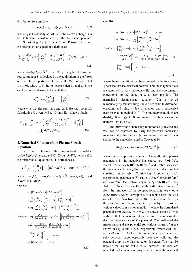
The mirror ratio increasing monotonically toward the

wall can be expressed by using the potential decreasing

monotonically. For the case (a), we assume the mirror ratio

similar to the expression used by Sato et al. [4]

!

R(") = exp # " $ e%w /(kTe){ }1/ 2[ ] , (24)

where α is a positive constant. Generally the plasma

parameters in the negative ion source are Te=1~5eV,

Ti=0.3~0.5eV, ne=3×1011~3×1012cm-3 and spatial scales of

the three sides of the negative ion source is about several ten

cm~1m, respectively. Considering Horiike et al.’s

experimental parameters [8], that is, Te=2eV, ne=2×1012cm-3

and L=7.9cm, the Debye length is λD~7.4×10-4cm, then

λD/L~10-4. Since we use the mesh width Δs=Δz/L=2×10-2

from the limitation of the computational time, we choose

λD/L=5×10--2, which corresponds to a region near the wall

(about 1.5×10--2cm from the wall). The relation between

the potential and the mirror ratio given by Eq. (24) for

various values of α is shown in Fig. 4, where the normalized

potential ψ=η−eφw/(kTe)=−eφ/(kTe) is shown instead of η. It

is shown that the increase rate of the mirror ratio is smaller

than the decrease rate of the potential. The profiles of the

mirror ratio and the potential for various values of α are

shown in Fig. 5 and Fig. 6, respectively, where Z=1, τ=1

and λD/L=5x10−2. As the value of α increases, the mirror

ratio becomes large, especially near the wall, and the

potential drop in the plasma region decreases. This may be

because that as the value of α increases, the ions are

reflected by the increasing magnetic field near the wall and

601


Fig.4 Relation between the normalized potential ψ = −eφ/kTe and

the mirror ratio R given by Eq. (24) for various values of α

(case (a)).

Fig.5 Profile of the mirror ratio R for various values of α with

λD/L=5x10-2 (case (a)).

Fig.6 Profile of the normalized potential ψ=−ef/kTe for various

values of α with λD/L=5x10-2 (case (a)).

Fig.7 Profile of the normalized potential ψ = −eφ/kTe for various

values of the temperature rate τ =Te/Ti with λD/L=5x10-2

(case (a)).

Fig.8 Relation between the normalized potential ψ=-eφ/kTe and

the mirror ratio R give by Eq. (25) for various values of α

(case (b)).

reciprocated between the two turning points. As a result, the

ions in the plasma region increase and the potential drop

decrease. The profile of the potential for various values of

the temperature ratio τ=Te/Ti is shown in Fig. 7, where Z=1,

α=0.4 and λD/L=5x10-2. As the value of τ increases, the

potential drop in the plasma region decreases. It may be

because that the low energy ions are reflected by the strong

magnetic field near the wall and reciprocated between the

two turning points. As a result, the ions in the plasma region

increase and the potential drop decreases.

On the other hand, for the case (b), we assume the

mirror ratio to be given by [4]

!

R(") = exp # " $ e%w /(kTe){ }[ ] . (25)

The relation between the potential and the mirror ratio given

by Eq. (25) for various values of α is shown in Fig. 8. It is

shown that the increase rate of the mirror ratio is larger than

the decrease rate of the potential. The profiles of the mirror

ratio and the potential for various values of α are shown in

Fig. 9 and Fig. 10, respectively, where Z=1, τ=1 and

λD/L=5x10−2. It is shown that as the value of α increases, the

mirror ratio becomes large, especially near the wall more

than the case (a). Although as the value of α increases the

potential drop decreases, dependence of the potential profile

on the value of α is smaller than the case (a). This may be

because that a reflection effect of the potential on the ions is

smaller than the case (a). In the case (a) the ions are

reflected by the increasing magnetic field near the wall and

reciprocated between the two turning points, at the same

time the ions are reflected by the potential near the wall. On

the other hand, in the case (b), since the decrease rate of the

potential is smaller than the increase rate of the magnetic

field toward the wall, the reflection effect on the ions by the

potential is smaller than the case (a). In a result, reflected

602


Fig.9 Profile of the mirror ratio R for various values of α with λD/L=5x10-2 (case (b)).

Fig.10 Profile of the normalized potential ψ =−eφ/kTe for various

values of α with λD/L=5x10-2 (case (b)).

Fig.11 Profile of the normalized potential ψ =−eφ/kTe for various

values of the temperature rate τ =Te/Ti with λD/L=5x10-2

(case (b)).

ions decrease and the potential drop in the plasma region

increases compared with the case (a). The profiles of the

potential for various values of the temperature ratio τ=Te/Ti

is shown in Fig. 11, where Z=1, α=0.4 and λD/L=5x10-2. As

the value of τ increases, the potential drop decreases same as

the case (a), though the potential drop is a little larger than

the case (a). This may be also because that the reflection

effect of the potential on the ions is smaller than the case (a).

5. Conclusions

The electric potential near the wall has been

investigated by considering the magnetic field increasing

toward the wall. The profile of the potential has been

obtained by solving the plasma-sheath equation. The

potential drop in the plasma region depends on the profile of

the magnetic field and the ion temperature. As the magnetic

field near the wall increases and the ratio of the ion

temperature to the electron temperature decreases, the

potential drop in the plasma region decreases. Furthermore,

the potential drop in the plasma region in the magnetic field

of which increase rate is larger than the decrease rate of the

potential becomes large compared with that in the magnetic

field of which increase rate is smaller than the decrease rate

of the potential. On the other hand, dependence of the

potential in the sheath region on the profile of the magnetic

field and the ion temperature is small.

As far as the results for the case (i) are concerned,

however, they are based on the relatively simple assumption

that the trapped ions are untrapped and lost from the system

after their one trapped orbit due to statistical process, e.g.,

collision process. Realistic modeling for such a collision

process is essential and will be included in the modeling in

the future to obtain more robust results for the case (i).

[1] A. Fukano, A. Hatayama and M. Ogasawara, JJAP 46, No.

4A, 1668(2004).

[2] V. E. Golant, A. P. Zhilinsky and I. E. Sakharov:

Fundamentals of Plasma Physics. (John Wiley and Sons,

New York, 1980).

[3] G. A. Emmert, R. M. Wieland, A. T. Mense, and J. N.

Davidson, Phys. Fluids 23,803(1980)

[4] K. Sato, F. Miyawaki, and W. Fukui, Phys. Fluids B1,

725(1989).

[5] M. Abramowitz and I. Stegun, Handbook of Mathematical

Functions (Dover, New York, 1974) p. 692.

[6] J. H. Whealton, E. F. Jaegar, and J. C. Whitson, J. Comput.

Phys. 27, 32 (1978).

[7] J. C. Whitson, J. Smith, and J. H. Whealton, J. Comput. Phys.

28, 408 (1978).

[8] H. Horiike, M. Akiba, Y. Ohara, Y. Okumura and S. Tanaka,

Phys. Fluids 30, 3268(1987).

603


electric potential in plasma and sheath regions with ... · author’s e-mail:...

Documents