ELE539A: Optimization of Communication Systems

Lecture 18: Algorithms for Unconstrained

Optimization

Professor M. Chiang

Electrical Engineering Department, Princeton University

March 27, 2006

Lecture Outline

• Unconstrained minimization problems

• Gradient method

• Newton method

• Equality constrained minimization problems

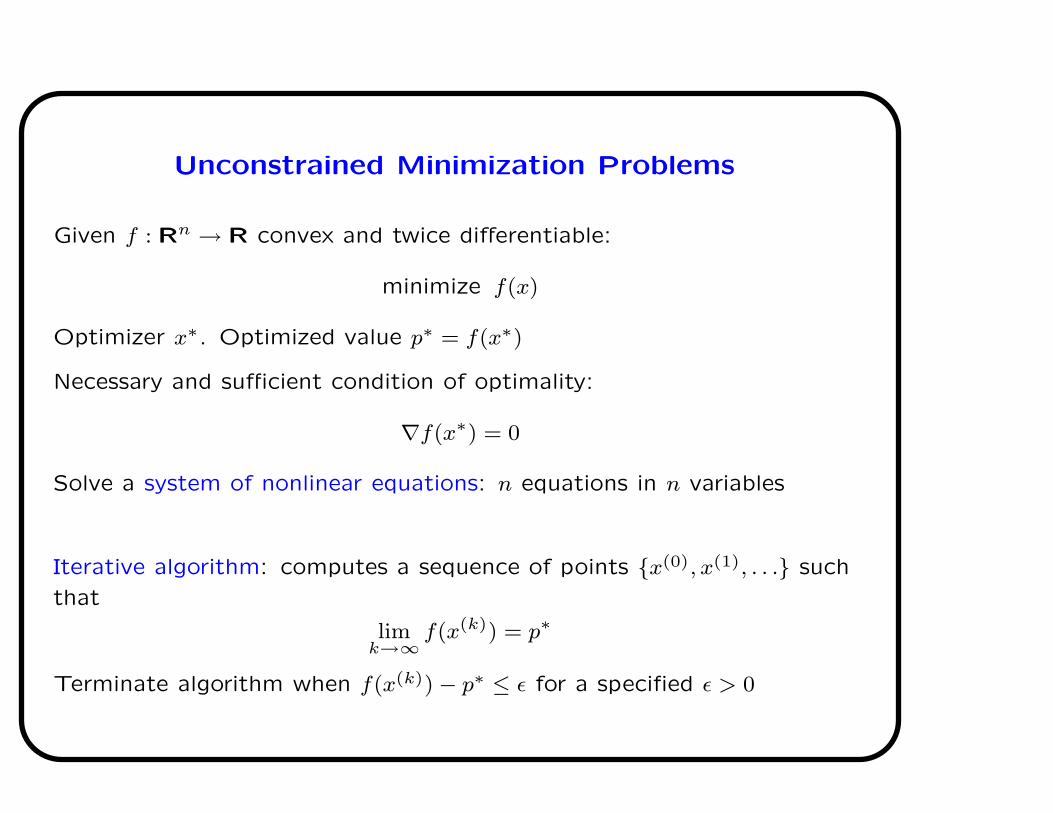
Unconstrained Minimization Problems

Given f : Rn → R convex and twice differentiable:

minimize f(x)

Optimizer x∗. Optimized value p∗ = f(x∗)

Necessary and sufficient condition of optimality:

∇f(x∗) = 0

Solve a system of nonlinear equations: n equations in n variables

Iterative algorithm: computes a sequence of points {x(0), x(1), . . .} such

that

limk→∞

f(x(k)) = p∗

Terminate algorithm when f(x(k)) − p∗ ≤ ǫ for a specified ǫ > 0

Examples

• Least-squares: minimize

‖Ax − b‖22 = xT (AT A)x − 2(AT b)T x + bT b

Optimality condition is system of linear equations:

AT Ax∗ = AT b

called normal equations for least-squares

• Unconstrained geometric programming: minimize

f(x) = log

mX

i=1

exp(aTi x + bi)

!

Optimality condition has no analytic solution:

∇f(x∗) =1

Pmj=1 exp(aT

j x∗ + bj)

mX

i=1

exp(aTi x∗ + bi)ai = 0

Strong Convexity

f assumed to be strongly convex: there exits m > 0 such that

∇2f(x) � mI

which also implies that there exists M ≥ m such that

∇2f(x) � MI

Bound optimal value:

f(x) −1

2m‖∇f(x)‖2

2 ≤ p∗ ≤ f(x) −1

2M‖∇f(x)‖2

2

Suboptimality condition:

‖∇f(x)‖2 ≤ (2mǫ)1/2 ⇒ f(x) − p∗ ≤ ǫ

Distance between x and optimal x∗:

‖x − x∗‖2 ≤2

m‖∇f(x)‖2

Descent Methods

Minimizing sequence x(k), k = 1, . . . , (where t(k) > 0)

x(k+1) = x(k) + t(k)∆x(k)

∆x(k): search direction

t(k): step size

Descent methods:

f(x(k+1)) < f(x(k))

By convexity of f , search direction must make an acute angle with

negative gradient:

∇f(x(k))T ∆x(k) < 0

Because otherwise, f(x(k+1)) ≥ f(x(k)) since

f(x(k+1)) ≥ f(x(k)) + ∇f(x(k))T (xk+1) − x(k))

General Descent Method

GIVEN a starting point x ∈ dom f

REPEAT

1. Determine a descent direction ∆x

2. Line search: choose a step size t > 0

3. Update: x := x + t∆x

UNTIL stopping criterion satisfied

Line Search

• Exact line search:

t = argmins≥0

f(x + s∆x)

• Backtracking line search:

GIVEN a descent direction ∆x for f at x, α ∈ (0, 0.5), β ∈ (0, 1)

t := 1

WHILE f(x) − f(x + t∆x) < α|∇f(x)T (t∆x)|, t := βt

Caution: t such that x + t∆x ∈ dom f

Gradient Descent Method

GIVEN a starting point x ∈ dom f

REPEAT

1. ∆x := −∇f(x)

2. Line search: choose a step size t > 0

3. Update: x := x + t∆x

UNTIL stopping criterion satisfied

Theorem: we have f(x(k)) − p∗ ≤ ǫ after at most

log((f(x(0)) − p∗)/ǫ)

log“

11−m/M

”

iterations of gradient method with exact line search

Example in R2

minimize f(x) =1

2(x2

1 + γx22), x∗ = (0, 0)

Gradient descent with exact line search:

x(k)1 = γ

„

γ − 1

γ + 1

«k

, x(k)2 =

„

−γ − 1

γ + 1

«k

−10 0 10

−4

0

4

x0

x1

x1

x2

Example in R2

x0

x1

x2

0 5 10 15 20 2510

−15

10−10

10−5

100

105

b

k

erro

rx

Which error decay curve is by backtracking and which is by exact line

search?

Observations

• Exhibits approximately linear convergence (error f(x(k)) − p∗ converges

to zero as a geometric series)

• Choice of α, β in backtracking line search has a noticeable but not

dramatic effect on convergence speed

• Exact line search improves convergence, but not always with

significant effect

• Convergence speed depends heavily on condition number of Hessian

Newton Method

Newton step:

∆xnt = −∇2f(x)−1∇f(x)

Positive definiteness of ∇2f(x) implies that ∆xnt is a descent direction

Interpretation: linearize optimality condition ∇f(x∗) = 0 near x,

∇f(x + v) ≈ ∇f(x) + ∇2f(x)v = 0

Solving this linear equation in v, obtain v = ∆xnt. Newton step is the

addition needed to x to satisfy linearized optimality condition

Main Properties

• Affine invariance: given nonsingular T ∈ Rn×n and let f̄(y) = f(Tx).

Then Newton step for f̄ at y:

∆ynt = T−1∆xnt

and

x + ∆xnt = T (y + ∆ynt)

• Newton decrement:

λ(x) =“

∇f(x)T∇2f(x)−1∇f(x)”1/2

=“

∆xTnt∇

2f(x)∆xnt

”1/2

Let f̂ be second order approximation of f at x. Then

f(x) − p∗ ≈ f(x) − infy

f̂(y) = f(x) − f̂(x + ∆xnt) =1

2λ(x)2

Newton Method

GIVEN a starting point x ∈ dom f and tolerance ǫ > 0

REPEAT

1. Compute Newton step and decrement: ∆xnt = −∇2f(x)−1∇f(x) and

λ =`

∇f(x)T∇2f(x)−1∇f(x)´1/2

2. Stopping criterion: QUIT if λ2

2≤ ǫ

3. Line search: choose a step size t > 0

4. Update: x := x + t∆x

Advantages of Newton method: Fast, Robust, Scalable

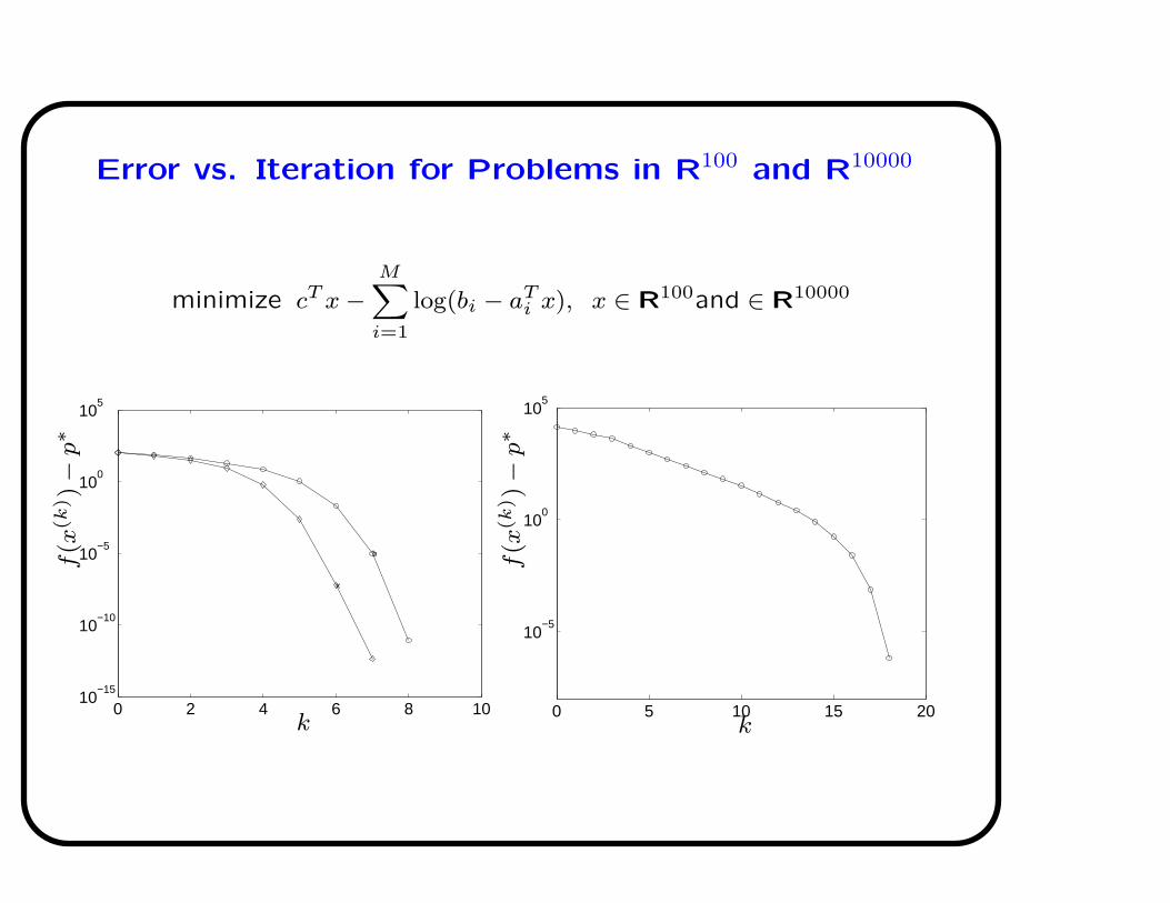
Error vs. Iteration for Problems in R100 and R10000

minimize cT x −MX

i=1

log(bi − aTi x), x ∈ R100and ∈ R10000

0 2 4 6 8 1010

−15

10−10

10−5

100

105

b

x

k

f(x

(k))−

p∗

0 5 10 15 20

10−5

100

105

k

f(x

(k))−

p∗

Equality Constrained Problems

Solve a convex optimization with equality constraints:

minimize f(x)

subject to Ax = b

f : Rn → R is twice differentiable

A ∈ Rp×n with rank p < n

Optimality condition: KKT equations with n + p equations in n + p

variables x∗, ν∗:

Ax∗ = b, ∇f(x∗) + AT ν∗ = 0

Approach 1: Can be turned into an unconstrained optimization, after

eliminating the equality constraints

Example With Analytic Solution

Convex quadratic minimization over equality constraints:

minimize (1/2)xT Px + qT x + r

subject to Ax = b

Optimality condition:

2

4

P AT

A 0

3

5

2

4

x∗

ν∗

3

5 =

2

4

−q

b

3

5

If KKT matrix is nonsingular, there is a unique optimal primal-dual pair

x∗, ν∗

If KKT matrix is singular but solvable, any solution gives optimal x∗, ν∗

If KKT matrix has no solution, primal problem is unbounded below

Approach 2: Dual Solution

Dual function:

g(ν) = −bT ν − f∗(−AT ν)

Dual problem:

maximize − bT ν − f∗(−AT ν)

Example: solve

minimize −Pn

i=1 log xi

subject to Ax = b

Dual problem:

maximize − bT ν +nX

i=1

log(AT ν)i

Recover primal variable from dual variable:

xi(ν) = 1/(AT ν)i

Approach 3: Direct Derivation of Newton Method

Make sure initial point is feasible and A∆xnt = 0

Replace objective with second order Tayler approximation near x:

minimize f̂(x + v) = f(x) + ∇f(x)T v + (1/2)vT ∇2f(x)v

subject to A(x + v) = b

Find Newton step ∆xnt by solving:

2

4

∇2f(x) AT

A 0

3

5

2

4

∆xnt

w

3

5 =

2

4

−∇f(x)

0

3

5

where w is associated optimal dual variable of Ax = b

Newton’s method (Newton decrement, affine invariance, and stopping

criterion) stay the same

Lecture Summary

• Iterative algorithm with descent steps for unconstrained minimization

problems

• Gradient method and Newton method

• Convert equality constrained optimization into unconstrained

optimization

Chapters 9.1-9.3, 9.5 and 10.1-10.2 in Boyd and Vandenberghe