Elasticity & DiscretizationJan 11, 2016

Logistics

• I’ve created and posted the schedule based on sign-ups.

• 1st review due Sunday at 5pm; pick one of the 4 rigid body papers from the schedule. Submit your review to the LEARN DropBox.

• Other?

Elasticity

Elasticity

An elastic object is one that, when deformed, seeks to return to its original reference or rest configuration.

Previously: we saw discrete mass/spring models.Today: more principled continuum mechanics approach.

Generalizes 1D elasticity (springs) to 3D objects.

Will loosely follow Sifakis’ SIGGRAPH course: http://run.usc.edu/femdefo/sifakis-courseNotes-TheoryAndDiscretization.pdf

Continuum Mechanics

View the material under consideration as a continuous mass, rather than a set of discrete particles/atoms.

Useful for both solids and fluids.

Not always applicable: e.g., at small scales, during some kinds of fracture, for objects that are composed of large discrete elements, etc.

v.s.

Elasticity - Springs

Recall: The linear spring force is dictated by displacement, ∆𝑥 = 𝐿 − 𝐿0, away from rest length (Hooke’s law):

𝐹 = −𝑘∆𝑥.

This force is related to the spring’s potential energy:

U =1

2𝑘(∆𝑥)2.

The force acts to drive potential energy towards zero, by reducing the displacement, ∆𝑥.

Conservative Forces

The spring force is an example of a conservative force – it depends only on the current state (i.e., it is “path-independent”).

In this case, the force 𝐹 is given by the gradient of a potential energy 𝑈:𝐹 = −𝛻𝑈.

For our continuum elastic material, we seek a potential energy that is zero when our 3D object is undeformed.

Elasticity – 3D

How can we generalize the spring to (three-dimensional) volumes of material?

First, we need a way to describe 3D deformations.

Deformation Map

A function 𝜙 that maps points from the reference configuration ( 𝑋) to current position in world space ( 𝑥).

𝜙: ℝ3 → ℝ3

Purpose is similar to the state/transform of a rigid body.

However, each (infinitesimal) point in the body can now have a different transformation.

Deformation Map, 𝜙

𝜙: ℝ3 → ℝ3

𝑋 𝑥 = 𝜙(𝑋)

Reference/rest/undeformedconfiguration:

World/deformed configuration:

Deformations

The deformation map says where points in the material have moved to.

However, to determine forces due to deformation, we need to know how nearby points have moved relative to one another.

The tool we need is the deformation gradient.

Deformation Gradient, 𝐹 =𝜕𝜙

𝜕𝑋

𝑋

𝑥

𝑋 + 𝑑𝑋 𝑥 + 𝑑𝑥

𝜙: ℝ3 → ℝ3

Reference/rest/undeformedconfiguration:

World/deformed configuration:

Deformation Gradient

For some offset position from 𝑋, say 𝑋 + 𝑑𝑋, what is the corresponding world position?

𝑥 + 𝑑𝑥 = 𝜙 𝑋 + 𝑑𝑋 ≈ 𝜙 𝑋 +𝜕𝜙

𝜕 𝑋𝑑𝑋 = 𝑥 + 𝑭𝑑𝑋

Deformation gradient, 𝑭 =𝜕𝜙

𝜕𝑋, describes how particle positions have

changed relative to one another.

Offset in rest space

Taylor expand… Deformation gradient

Deformation Gradient

It is given by the 3 × 3 matrix (tensor):

𝑭 =𝜕𝜙

𝜕 𝑋=

𝜕𝜙1

𝜕𝑋1

𝜕𝜙1

𝜕𝑋2

𝜕𝜙1

𝜕𝑋3𝜕𝜙2

𝜕𝑋1

𝜕𝜙2

𝜕𝑋2

𝜕𝜙2

𝜕𝑋3𝜕𝜙3

𝜕𝑋1

𝜕𝜙3

𝜕𝑋2

𝜕𝜙3

𝜕𝑋3

Deformation Gradient: 𝑭 =𝜕𝜙

𝜕𝑋

Examples of simple deformations:Translation: 𝑥 = 𝜙( 𝑋) = 𝑡 + 𝑋, implies 𝑭 = 𝐼.

• World pos 𝑥 is rest pos 𝑋 plus a translation, 𝑡. Zero relative motion between points.

Uniform Scaling: 𝑥 = 𝜙 𝑋 = 𝑠𝑋 implies 𝑭 = 𝑠𝐼.

• World pos 𝑥 is rest pos 𝑋 times a constant, 𝑠.

Rotation: 𝑥 = 𝜙 𝑋 = 𝑅𝑋 implies 𝑭 = 𝑅.

• World pos 𝑥 is rest pos 𝑋 rotated by matrix 𝑅.

One Possible Potential Energy

What if we use 𝑭 directly to construct a potential energy?

U 𝑭 =𝑘

2𝑭 − 𝐼 𝐹

2

Resulting forces (−∇U) will drive 𝑭 towards 𝐼, i.e., a deformation that is (just) a translation.

What’s wrong with this?

Frobenius norm, 𝑨 𝐹 = 𝑖 𝑗 𝑎𝑖,𝑗2

Strain Measures

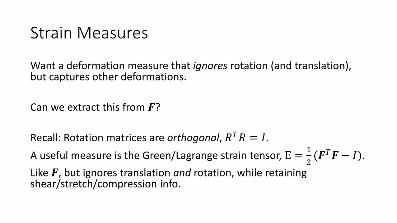
Want a deformation measure that ignores rotation (and translation), but captures other deformations.

Can we extract this from 𝑭?

Recall: Rotation matrices are orthogonal, 𝑅𝑇𝑅 = 𝐼.

A useful measure is the Green/Lagrange strain tensor, E =1

2(𝑭𝑇𝑭 − 𝐼).

Like 𝑭, but ignores translation and rotation, while retaining shear/stretch/compression info.

Strain Measures

But, Green strain is nonlinear (quadratic), so more costly.

For small deformations, can use small/infinitesimal/Cauchy strain:

𝜖 =1

2(𝑭𝑇 + 𝑭) − 𝐼

(A linearization of Green strain.)

Many other strain tensors exist (and these two have many names)…

Big Picture – So Far

• Deformation map 𝜙 describes map from rest to world state.

• Deformation gradient 𝑭 =𝜕𝜙

𝜕𝑋describes deformation (minus translation).

• Strains 𝜖 or E describe deformation (minus rotation).

• Then what…

Remaining questions:

• What are the equations of motion (“𝐹 = 𝑚𝑎") for our continuous blob of material?

• How to get from strains to forces?

Equations of Motion

Consider 𝐹 = 𝑚𝑎 for a small, continuous “blob” of material.

Ω

𝐹𝑏𝑜𝑑𝑦𝑑𝑋 + 𝜕Ω

𝑇𝑑𝑆 = Ω

𝜌 𝑥𝑑𝑋

𝐹𝑏𝑜𝑑𝑦: “body” forces that act throughout the material (e.g. gravity, magnetism, etc.). i.e., force per unit volume (i.e., force density).

𝑇: tractions, i.e., force per unit area acting on a surface.

𝜌: density.

Ω is the material region being considered, with surface/boundary 𝜕Ω.

Traction

Traction T is a force (vector) per unit area on a small piece of surface.

𝑇( 𝑋, 𝑛) = lim𝐴→0

𝐹

𝐴

Cauchy’s postulate:

Traction is a function of position 𝑋 and normal 𝑛.

i.e., doesn’t depend on curvature, area or other properties.

Consists of normal/pressure component along 𝑛, and tangential/shear components perpendicular to it.

𝑛 𝑇

Traction

Consider the internal traction on any slice through a volume of material.

This describes the forces acting on this plane between the two “sides”.

Note: 𝑇(𝑥, 𝑛) = −𝑇(𝑥, −𝑛) (by Newton’s 3rd).

Traction

We can characterize internal forces by considering tractions on 3 perpendicular slices (i.e., normals along 𝑥, 𝑦, 𝑧, directions).

3 components per traction along 3 axes gives us 9 components.

This gives us the Cauchy stress tensor, 𝜎.

Traction on any plane can be recovered via𝑇 = 𝜎𝑛

where 𝑛 is the normal of the plane.

Stress

The 3 × 3 stress tensor describes all the forces acting within a material (at a given point).

𝜎 =

𝜎𝑥𝑥 𝜎𝑥𝑦 𝜎𝑥𝑧𝜎𝑦𝑥 𝜎𝑦𝑦 𝜎𝑦𝑧𝜎𝑧𝑥 𝜎𝑧𝑦 𝜎𝑧𝑧

𝜎 can be shown to be symmetric, i.e., 𝜎𝑦𝑥 = 𝜎𝑥𝑦, etc. (from conservation of angular momentum.)

Stress – Physical meaning?

Diagonal components correspond to compression/extension (normal) forces.

Off-diagonal components correspond to shear forces.

Equations of motion

Ω

𝐹𝑏𝑜𝑑𝑦𝑑𝑋 + 𝜕Ω

𝑇𝑑𝑆 = Ω

𝜌 𝑥𝑑𝑋

• Plug in 𝑇 = 𝜎𝑛…

Ω

𝐹𝑏𝑜𝑑𝑦𝑑𝑋 + 𝜕Ω

𝜎𝑛𝑑𝑆 = Ω

𝜌 𝑥𝑑𝑋

• Integrate by parts (divergence theorem) to eliminate surface integral:

Ω

𝐹𝑏𝑜𝑑𝑦𝑑𝑋 + Ω

𝛻 ∙ 𝜎𝑑𝑋 = Ω

𝜌 𝑥𝑑𝑋

In limit of small Ω, 𝐹𝑏𝑜𝑑𝑦 + 𝛻 ∙ 𝜎 = 𝜌 𝑥, for every infinitesimal point.

Big Picture – So Far

• Deformation map 𝜙 describes map from rest to world state

• Deformation gradient 𝐹= describes deformations (minus translation)

• Strains 𝜖 or E describe deformation (minus rotation)

• Stress 𝜎 describes forces in material

• PDE 𝐹𝑏𝑜𝑑𝑦 + 𝛻 ∙ 𝜎 = 𝜌 𝑥 describes how to apply stress to get motion

• (Later, will discretize the PDE to get discrete equations to solve.)

Last missing step!

Constitutive models

Strain E/ 𝜖 describes deformations of a body.

Stress 𝜎 describes (resulting) forces within a body.

Constitutive models dictate the stress-strain relationship in a material.

i.e., Given some deformation, what stresses (forces) does it induce?

e.g., Explains why rubber responds differently than concrete.

Linear Elasticity - simplest isotropic model

Hooke’s law in 3D, for small strain, 𝜖.

Potential Energy:

𝑈 𝐹 = 𝜇𝜖: 𝜖 +𝜆

2tr2(𝜖)

Stress:𝜎 = 2𝜇𝜖 + 𝜆tr(𝜖)𝐼

𝜇, 𝜆 are the Lamé parameters, loosely analogous to 1D spring stiffness 𝑘.“tr” is the trace operator (sum of diagonals of tensor/matrix)

“:” is a tensor double dot product, where 𝐴: 𝐵 = tr(𝐴𝑇𝐵)

(i.e., behaves the same in all directions.)

Linear Elasticity

Derives from the simplest possible linear relationship between 𝜎 and 𝜖.

• Flatten the 3x3 tensors 𝜖 and 𝜎 into vectors.

• Isotropy and symmetry of 𝜖/𝜎 reduce 81 coeffs down to 2 independent parameters (e.g., 𝜇 and 𝜆).

𝜎𝑥𝑥𝜎𝑥𝑦𝜎𝑥𝑧𝜎𝑦𝑥𝜎𝑦𝑦𝜎𝑦𝑧𝜎𝑧𝑥𝜎𝑧𝑦𝜎𝑧𝑧

= 9𝑥9 𝑐𝑜𝑒𝑓𝑓𝑖𝑐𝑖𝑒𝑛𝑡 𝑚𝑎𝑡𝑟𝑖𝑥

𝜖𝑥𝑥𝜖𝑥𝑦𝜖𝑥𝑧𝜖𝑦𝑥𝜖𝑦𝑦𝜖𝑦𝑧𝜖𝑧𝑥𝜖𝑧𝑦𝜖𝑧𝑧

Other Elastic moduli

A more common/intuitive (but interconvertible) parameter pair is Poisson’s ratio, 𝜈, and Young’s modulus, E, or Y. (Careful overloading E).

𝜇 =𝑌

2(1 + 𝜈)

and…

𝜆 =𝑌𝜈

(1 + 𝜈)(1 − 2𝜈)

Elastic Moduli – Young’s modulus

Young’s modulus:

• Ratio of stress-to-strain along an axis.

• Should be consistent with linear spring.

Elastic Moduli – Poisson’s ratio

• Poisson’s ratio is negative ratio of transverse to axial strain• If stretched in one direction, how much does it compress in the others?

• Expresses tendency to preserve volume.

• Lies in range [−1, 0.5].

• 0.5 = incompressible (e.g., rubber)

• 0 = no compression (e.g., cork)

• < 0 is possible, though weird...

• Called auxetic materials.

The “linear” in linear elasticity

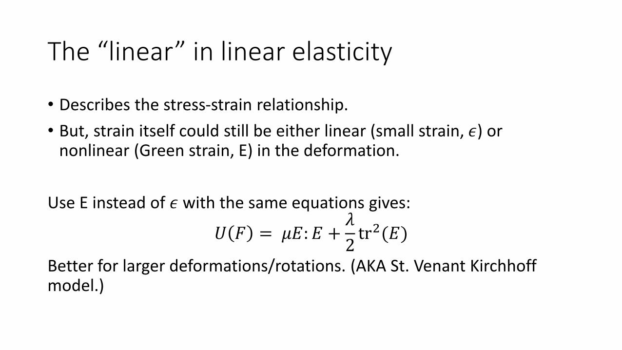
• Describes the stress-strain relationship.

• But, strain itself could still be either linear (small strain, 𝜖) or nonlinear (Green strain, E) in the deformation.

Use E instead of 𝜖 with the same equations gives:

𝑈 𝐹 = 𝜇𝐸: 𝐸 +𝜆

2tr2(𝐸)

Better for larger deformations/rotations. (AKA St. Venant Kirchhoff model.)

Other common models

• Corotational linear elasticity:• Try to pre-factor out the rotational part of strain in a different way; treat the

remainder with linear elasticity.

• We’ll see this idea in the “Interactive Virtual Materials” paper.

• Neo-Hookean elasticity:• St.V-K breaks down under large compression (stops resisting).

• Neo-Hookean is a nonlinear model that corrects this.

A Taste of Common Discretization Methods

Discretization

Need to turn our continuous model describing infinitesimal points…

𝐹𝑏𝑜𝑑𝑦 + 𝛻 ∙ 𝜎 = 𝜌 𝑥

…into a discrete model that approximates it (and can be computed!)

Standard choices: Finite difference (FDM), finite volume (FVM), and finite element methods (FEM).

I’ll give a brief flavour, but… there’s a vast literature & theory. (See e.g. Numerical PDE course, CS778.)

Finite differences

Dice the material/domain into a grid of points

holding the relevant data.

Replace all (continuous, spatial) derivatives with (discrete) finite difference approximations.

e.g., 𝑑𝑦

𝑑𝑥≈𝑦 𝑥 + ∆𝑥 − 𝑦 𝑥

∆𝑥

Time Discretization

• Notice: Time integration schemes (FE, RK2, BE, etc.) are discretizations of time derivatives, along the 1D time axis.

• E.g., Forward Euler uses a 1st order (one-sided) finite difference:𝑑𝑥

𝑑𝑡≈𝑥𝑖+1 − 𝑥𝑖

Δ𝑡

• We distinguish time discretization and spatial discretization, and focus on the latter now.

e.g. 1D Heat equation

Continuous equation: 𝜕𝜙

𝜕𝑡− 𝛼

𝜕2𝜙

𝜕𝑥2= 0

Discretize time derivative (w/ forward Euler):

𝜙𝑡+Δ𝑡 = 𝜙𝑡 + Δ𝑡𝛼𝜕2𝜙𝑡

𝜕𝑥2

Discretize spatial derivatives with F.D.:

𝜙𝑡+Δ𝑡 = 𝜙𝑡 + Δ𝑡𝛼

𝜙𝑡𝑖+1 − 𝜙𝑡

𝑖

Δ𝑥−𝜙𝑡𝑖 − 𝜙𝑡

𝑖−1

Δ𝑥

Δ𝑥

e.g. 1D Heat(diffusion) equation

https://www.youtube.com/watch?v=mjDhdyxnOwo

Finite differences

Very common for fluids… less so for solids.

Few graphics papers use FDM for solids: e.g., “An efficient multigrid method for the simulation of high-resolution elastic solids”

Advantages: often simpler to implement, nice grid structure offers various optimizations, cache coherent memory accesses…

Disadvantages: trickier for irregular shapes and boundaries not aligned with axes

Finite volume

• Divide the physical domain up into a set of non-overlapping “control volumes.”

• Could be irregular, tetrahedra, hexahedra, general polyhedral, etc.

• Approximate the integrated/average value of quantities within the cell (rather than point values like F.D.).

• Consider the exchange of data between adjacent cells. Figure from the DistMesh gallery:

http://persson.berkeley.edu/distmesh/gallery_images.html

Finite volume – Conservation laws

Useful for conserved quantities; ensures the exact “flow” leaving one cell enters the next.

• E.g. mass, heat, momentum, etc.

Applies to equations in “conservation form”:𝑑𝜙

𝑑𝑡+ ∇ ⋅ 𝑓(𝜙) = 0

Particularly common for fluids.

Reminder: Divergence operator, ∇ ⋅

For vector field 𝑢( 𝑥), divergence is a signed scalar measuring net flow out of a point.

i.e. to what degree that point is a source (v.s. a sink) for the vector field.

∇ ⋅ 𝑢 =𝜕𝑢

𝜕𝑥+𝜕𝑣

𝜕𝑦+𝜕𝑤

𝜕𝑧

Flowing out: positive

Flowing in: negative

Neither: zero (“divergence-free”)

[Tong et al. 2003]

e.g. 1D Heat equation

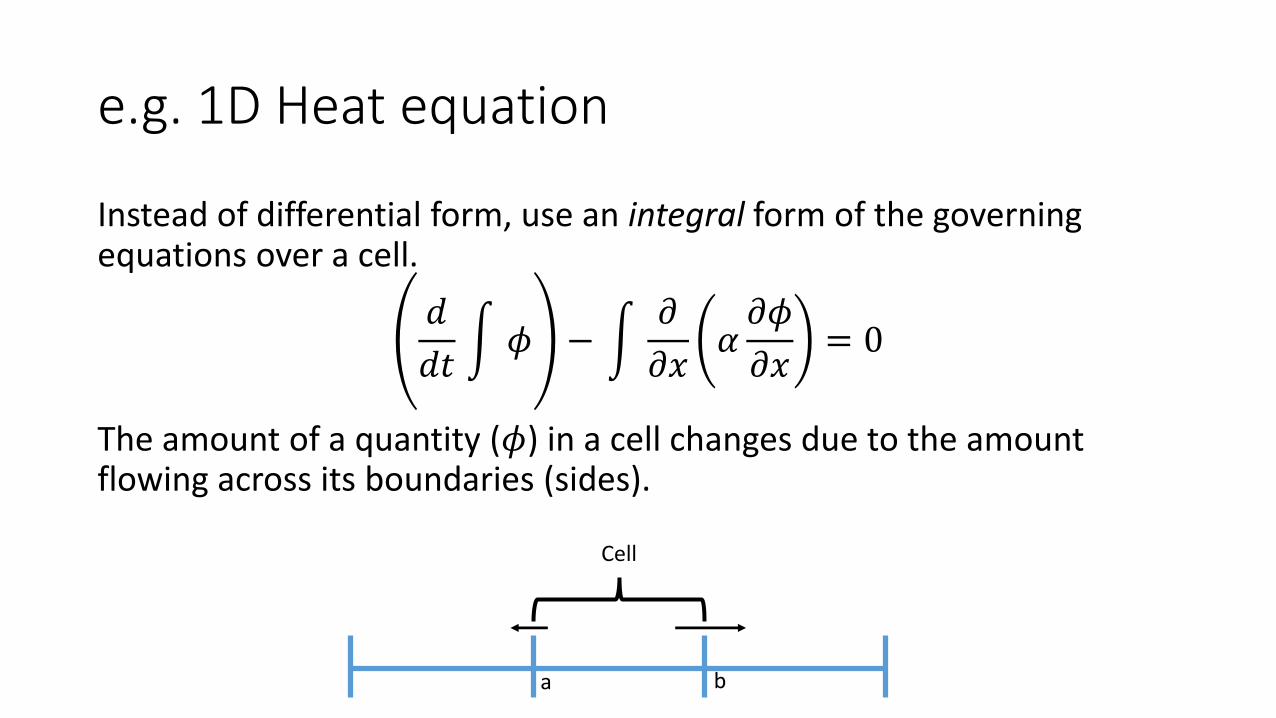
Instead of differential form, use an integral form of the governing equations over a cell.

𝑑

𝑑𝑡 𝜙 −

𝜕

𝜕𝑥𝛼𝜕𝜙

𝜕𝑥= 0

The amount of a quantity (𝜙) in a cell changes due to the amount flowing across its boundaries (sides).

Cell

a b

e.g. 1D Heat equation

𝑑

𝑑𝑡

𝑎

𝑏

𝜙𝑑𝑥 −

𝑎

𝑏𝜕

𝜕𝑥𝛼𝜕𝜙

𝜕𝑥𝑑𝑥 = 0 →

𝑑

𝑑𝑡

𝑎

𝑏

𝜙 𝑑𝑥 − 𝛼𝜕𝜙

𝜕𝑥𝑎

𝑏

= 0

We estimate the difference in “flux” 𝛼𝜕𝜙

𝜕𝑥at the right and left side of the cell.

This tells us how much the total 𝜙 in the cell, 𝑎𝑏𝜙𝑑𝑥, changes per unit

time. Cell

a b

By FTOC

Finite volume – Equations of motion

Return to the integral form of our equations of motion…

Ω

𝐹𝑏𝑜𝑑𝑦𝑑𝑋 + Ω

𝛻 ∙ 𝜎𝑑𝑋 = Ω

𝜌 𝑥𝑑𝑋

Convert divergence term into surface integrals by divergence th’m.

e.g. Ω 𝛻 ∙ 𝜎𝑑𝑋 = 𝜕Ω𝜎 ∙ 𝑛 𝑑𝑆

≈

𝑓𝑎𝑐𝑒𝑠 𝑓

(𝜎𝑓∙ 𝑛𝑓)𝐿𝑓

Integrate remaining terms to get volume-averaged quantities per cell.

𝑛𝑓 (normal)

𝐿𝑓 (length)

𝜎𝑓 (stress)

Finite volume – Elasticity

We’ll see details of FV applied to elastic objects in the paper:

“Finite Volume Methods for the Simulation of Skeletal Muscle”

Finite element methods

Core idea:

We can’t really solve the infinite dimensional, continuous problem describing all points in the material!

Instead find a solution that we can represent, in some finite dimensional subspace.

Concretely:

1. choose an approximate representation of continuous functions on a discrete mesh.

2. find the “best” solution possible among all functions that representation can describe.

Finite elements – basis functions

In 1D, consider the space of functions representable by (piecewise) linear interpolation on a set of grid points.

Just a linear combination of scaled and translated “hat” functions at each gridpoint, called a basis function.

Many others bases are possible (e.g. higher order polynomials).

Finite elements

Then, any function 𝑢 in this space can be described by:

𝑢 𝑥 =

𝑘=1

𝑛

𝑢𝑘𝑣𝑘(𝑥)

where 𝑢𝑖 are the coefficients, and 𝑣𝑘 𝑥 are the basis functions, (“hats” in our case.)

To find a solution to a problem, we want to find the discrete coefficients, 𝑢𝑘.

The approximated continuous solution is recovered by interpolation.

Higher dimensional functions

This generalizes to higher dimensions, where our scalar function 𝑢depends on multiple variables (e.g. 𝑥, 𝑦, 𝑧)

e.g., two dimensions:

2D mesh with numbered nodes. A single linear “hat” basis function in 2D.

Finite elements

Take a 1D model problem: 𝑑2𝑢

𝑑𝑥2= 𝑓 on [0,1], with 𝑢 0 = 0, 𝑢 1 =0.

For given 𝑓, find 𝑢.

For a proper solution, it will also be true that

𝑑2𝑢

𝑑𝑥2𝑣𝑑𝑥 = 𝑓𝑣𝑑𝑥

for all “test functions” 𝑣 (that are smooth and satisfy the BC).

We require this, rather than pointwise satisfaction of original equation.

Finite elements

Integrate LHS by parts (with zero boundaries) to get:

𝑑𝑢

𝑑𝑥

𝑑𝑣

𝑑𝑥𝑑𝑥 = 𝑓𝑣 𝑑𝑥

This is called the weak form of the PDE.

Now, we will replace 𝑢, 𝑓, and 𝑣 with our space of discrete, piecewise linear functions.

Finite elements

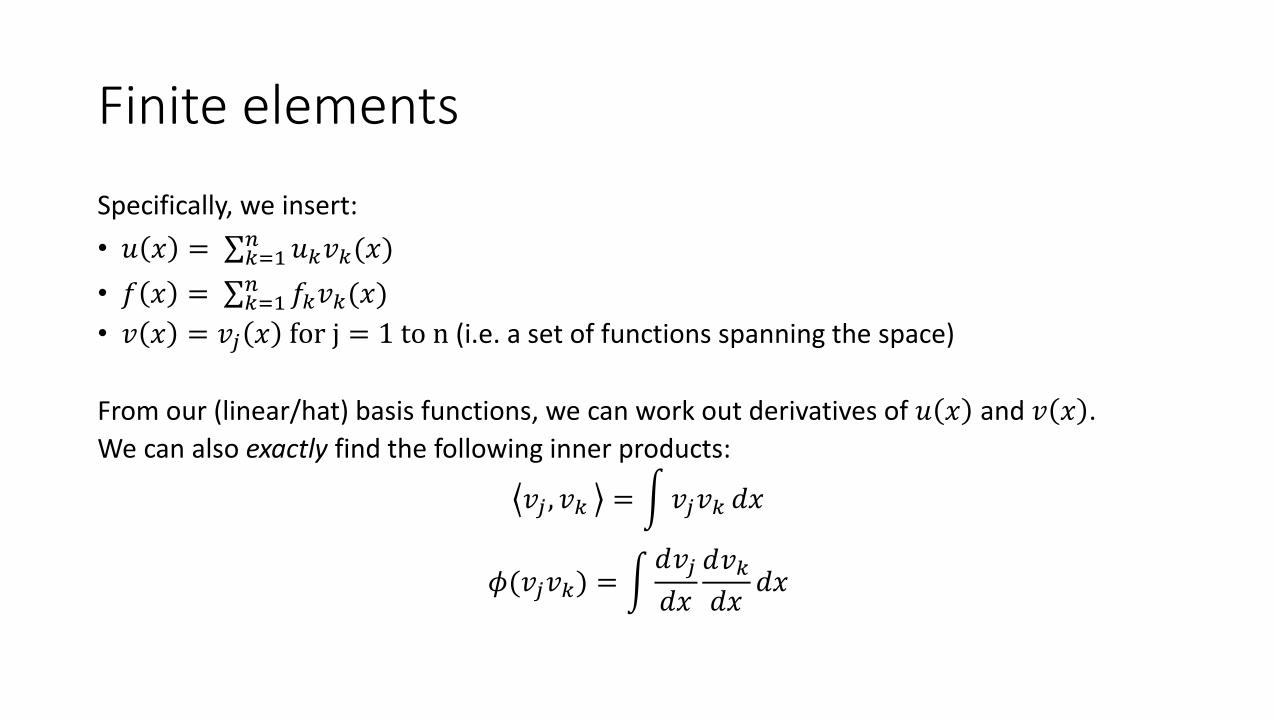
Specifically, we insert:

• 𝑢 𝑥 = 𝑘=1𝑛 𝑢𝑘𝑣𝑘(𝑥)

• 𝑓 𝑥 = 𝑘=1𝑛 𝑓𝑘𝑣𝑘(𝑥)

• 𝑣 𝑥 = 𝑣𝑗 𝑥 for j = 1 to n (i.e. a set of functions spanning the space)

From our (linear/hat) basis functions, we can work out derivatives of 𝑢 𝑥 and 𝑣 𝑥 .

We can also exactly find the following inner products:

𝑣𝑗 , 𝑣𝑘 = 𝑣𝑗𝑣𝑘 𝑑𝑥

𝜙(𝑣𝑗𝑣𝑘) = 𝑑𝑣𝑗

𝑑𝑥

𝑑𝑣𝑘𝑑𝑥

𝑑𝑥

Finite elements

After plugging into 𝑑𝑢

𝑑𝑥

𝑑𝑣

𝑑𝑥= 𝑓𝑣 and rearranging, this yields a set of n

discrete equations of the form:

Unknown coefficients

Known inner products

Known inner products

𝑘=1

𝑛

𝑢𝑘 𝜙 𝑣𝑗 , 𝑣𝑘 =

𝑘=1

𝑛

𝑓𝑘 𝑣𝑗 , 𝑣𝑘

Known input data

Final system

Letting 𝐮 be the vector of unknown coefficients, and 𝐛 the RHS vector, this becomes a matrix equation:

L𝐮 = 𝐛

where the entries of L are just the 𝜙 𝑣𝑗 , 𝑣𝑘 ’s we defined.

See paper “Graphical Modeling and Animation of Brittle Fracture” for details of an early application of FEM to elasticity in graphics.

Example – FEM with fracture

“Graphical modeling and animation of brittle fracture”, O’Brien et al. 1999

FD/FV/FE elasticity v.s. mass-spring

• In all cases (w/ implicit time integration) we get a possibly nonlinear system of equations to solve for data stored on a discrete mesh/grid.

• However, for FD/FV/FE: • we can use physically meaningful/measurable parameters.

• as the mesh resolution is increased, we approach true/real analytical solutions.

• behaviour becomes independent of the mesh structure (under refinement!)• E.g. eliminates bias due to triangle edge directions. With springs, the mesh structures

below behave differently regardless of how fine the mesh is.

Summary

• The equations of elasticity give us a more consistent and principled approach to evolving continuous deformable bodies.

• The most common approaches to discretizing the resulting PDE are the finite difference, volume, and element methods.