elastic-plastic fatigue crack growth analysis under
TRANSCRIPT

Elastic-Plastic Fatigue Crack Growth
Analysis under Variable Amplitude Loading
Spectra
by
Semen Mikheevskiy
A thesis
presented to the University of Waterloo
in fulfillment of the
thesis requirement for the degree of
Doctor of Philosophy
in
Mechanical Engineering
Waterloo, Ontario, Canada, 2009
© Semen Mikheevskiy 2009

ii
AUTHOR'S DECLARATION
I hereby declare that I am the sole author of this thesis. This is a true copy of the thesis, including any
required final revisions, as accepted by my examiners.
I understand that my thesis may be made electronically available to the public.

iii
Abstract
Most components or structures experience in service a variety of cyclic stresses. In the case
of cyclic constant amplitude loading the fatigue crack growth depends only on the crack, the
component geometry and the applied loading. In the case of variable amplitude loading it also
depends on the preceding cyclic loading history. Various types of load sequence (overloads,
under-loads, or combination of them) may induce different load-interaction effects which can
cause either acceleration or reduction of the fatigue crack growth rate.
The previously developed UniGrow fatigue crack growth model for constant amplitude
loading histories which was based on the analysis of the local stress-strain material behaviour at
the crack tip has been improved, modified and extended to such a level of sophistication that it
can be used for fatigue crack growth analyses of cracked bodies subjected to arbitrary variable
amplitude loading spectra. It was shown that the UniGrow model enables to correctly predict the
effect of the applied compressive stress and tensile overloads by accounting for the existence of
the internal (residual) stresses induced by the reversed cyclic plasticity around the crack tip. This
idea together with additional structural memory effect model has been formalized
mathematically and coded into computer program convenient for predicting fatigue crack growth
under arbitrary variable amplitude loading spectra.
The experimental verification of the proposed model was performed using 7075-T6, 2024-
T3, 2324-T7, 7010-T7, 7050-T7 aluminium alloys, Ti-17 titanium alloy, and 350WT steel. The
good agreement between theoretical and experimental data proved the ability of the UniGrow
model to predict fatigue crack growth and fatigue crack propagation life under a wide variety of
real variable amplitude loading spectra.

iv
Acknowledgements
I would like to thank my supervisor Professor Grzegorz Glinka for the scientific support,
helpful discussions, and useful comments.
The Office of Naval Research, USA and Dr. A.K.Vasudevan are gratefully acknowledged for
the financial support and technical guidance.
I would also like to thank all graduate and undergraduate students who, in any sense,
participated and helped me in my research work. In particular, I am grateful to Elena
Atroshchenko for her contribution into weight functions development, Aditya Chattopadhyay for
his time spent by reading and commenting my thesis, Maria El Zeghayar for gentle criticism of
the proposed model, and Mohammad Amin Eshraghi for his moral support.
Additionally I would like to acknowledge Jakub Schmidtke, Krzysztof Hebel and Jakub
Gawryjolek for the contribution into the UniGrow software development.

v
Dedication
This thesis is dedicated to Svetlana Magovskaya who has always supported me in my work.

vi
Table of Contents
List of Figures............................................................................................................................................. ix
List of Tables ............................................................................................................................................xiv
Nomenclature ............................................................................................................................................ xv
Chapter 1 Introduction and Research Objectives.................................................................................... 1
Chapter 2 Literature Review ..................................................................................................................... 4
2.1 The Linear Elastic Fracture Mechanics............................................................................................... 4
2.2 Constant Amplitude Fatigue Crack Growth Models........................................................................... 6
2.2.1 Fatigue Crack Growth equations proposed by Paris .................................................................... 7
2.2.2 Two-parameter models ................................................................................................................ 8
2.2.3 The crack closure model ............................................................................................................ 11
2.3 Variable Amplitude Fatigue Crack Growth Models ......................................................................... 13
2.3.1 The Crack tip blunting ............................................................................................................... 13
2.3.2 Residual stresses ........................................................................................................................ 14
2.3.3 The Crack tip plasticity .............................................................................................................. 15
2.3.4 The Plasticity induced crack closure.......................................................................................... 17
Chapter 3 The Two-Parameter Total Driving Force Model ................................................................. 24
3.1 Introduction and basic assumptions .................................................................................................. 24
3.2 Residual compressive stresses at the crack tip, the residual stress intensity factor, and the total stress
intensity parameters.................................................................................................................. 25
3.2.1 Linear Elastic analysis of stresses and strains ahead of the crack tip ........................................ 26
3.2.2 Linear Elastic analysis of stresses and strains ahead of the crack tip under compressive
minimum load ..................................................................................................................................... 27
3.2.3 Elastic-plastic stresses and strains ahead of the crack tip .......................................................... 29

vii
3.3 Residual compressive stresses near the crack tip .............................................................................. 31
3.3.1 Calculation of the residual stress intensity factor, ............................................................... 32 rK
3.3.2 The Total maximum stress intensity factor and total stress intensity range............................... 33
3.4 The Bilinear two parameters driving force ....................................................................................... 34
3.4.1 The average stress over the elementary material block.............................................................. 34
3.4.2 The Fatigue crack growth expression based on the SWT fatigue damage accumulation
parameter............................................................................................................................................. 35
Chapter 4 Determination of the Elementary Material Block Size, ρ* ................................................. 42
4.1 The Method based on the fatigue limit and the threshold stress intensity range; (Method #1) ........ 42
4.2 The Method based on the experimental fatigue crack growth data obtained at various stress ratios;
(Method #2).............................................................................................................................. 44
4.3 The Method based on the Manson-Coffin fatigue strain-life curve and limited fatigue crack growth
data; (Method #3) ..................................................................................................................... 46
4.4 Summary of methods for the determination of the ρ* parameter ..................................................... 49
4.5 The effect of the elementary material block size on the residual stress intensity factor ................... 50
Chapter 5 Two-parameter Total Driving Force Model for Variable Amplitude Loading Spectra –
the UniGrow Fatigue Crack Growth Model........................................................................................... 56
5.1 The Maximum stress memory effect ................................................................................................ 57
5.2 The resultant minimum stress field and the residual stress intensity factor...................................... 58
5.3 The UniGrow analysis of simple loading spectra ............................................................................. 61
5.3.1 Constant amplitude loading ....................................................................................................... 61
5.3.2 Constant amplitude loading history interrupted by a single overload or underload .................. 62
5.3.3 Loading spectra with single over- and uder-loads ..................................................................... 64
Chapter 6 Fatigue Crack Growth Analysis under Spectrum Loading – Predictions/Experiments .. 72

viii
6.1 Fatigue crack growth in the Ti-17 titanium alloy under constant amplitude loading spectra with
under-loads ............................................................................................................................... 75
6.2 Fatigue crack growth in the 350WT Steel specimens under constant amplitude loading spectra with
periodic overloads .................................................................................................................... 86
6.3 Fatigue crack growth in the Al 2024 T3 alloy specimens under step-wise loading spectra ............. 93
6.4 Fatigue crack growth in the Al 7010 T7 alloy under constant amplitude loading spectra with
overloads ................................................................................................................................ 101
6.5 Fatigue crack growth in the Al 7075 T6 alloy specimens under P3 aircraft loading spectra.......... 108
6.6 Fatigue crack growth in the Al 7050-T7 alloy under the F/A-18 aircraft loading spectrum .......... 116
6.7 Fatigue crack growth in the AL 2324-T3 alloy under the P3 aircraft loading spectrum ................ 122
Chapter 7 Conclusions and Future Recommendations ....................................................................... 136
Appendix The UniGrow Fatigue Crack Growth Software ................................................................. 138
Bibliography ............................................................................................................................................ 142

ix
List of Figures Figure 2-1: Sharp crack in a linear elastic domain...................................................................................... 19
Figure 2-2: Blunted crack in a linear elastic domain ................................................................................. 19
Figure 2-3: General Shape of the Fatigue Crack Growth Rate curve ......................................................... 20
Figure 2-4: Experimental FCG data for Al 7075 T6 alloy [71, 73] ............................................................ 20
Figure 2-5: FCG data for AL 7075 T6 alloy in terms of Forman’s driving force Eq. 2-5 .......................... 21
Figure 2-6: FCG data for AL 7075 T6 alloy in terms of Weertman’s driving force Eq. 2-7...................... 21
Figure 2-7: FCG data for AL 7075 T6 alloy in terms of Priddle’s driving force Eq. 2-8........................... 22
Figure 2-8: FCG data for AL 7075 T6 alloy in terms of Mc Evily’s driving force Eq. 2-9 ....................... 22
Figure 2-9: FCG data for AL 7075 T6 alloy in terms of Walker’s driving force Eq. 2-10......................... 23
Figure 2-10: Schematic of the Willenborg model....................................................................................... 23
Figure 3-1: Discrete material model ........................................................................................................... 40
Figure 3-2: Schematic of the Neuber rule ................................................................................................... 40
Figure 3-3: Stress distributions ahead of the crack tip at various load levels ............................................. 41
Figure 3-4: Residual stress distribution obtained using the Neuber rule; Al 7075 T6 alloy , ΔK=Kmax=10
MPa√m ..................................................................................................................................... 41
Figure 4-1: Estimation of the elementary material block size based on the experimental fatigue crack
growth data (Method #2).......................................................................................................... 52
Figure 4-2: Iteration process for the elementary material block size estimation based on the Method #2
using linear ‘master’ curve ....................................................................................................... 52
Figure 4-3: Analytical and fitted ‘master’ curves for Al 7075-T6 alloy (Exp. data [71, 73])..................... 53
Figure 4-4: Schematic of experimental fatigue crack growth rate data ...................................................... 53
Figure 4-5: Elementary material block size as a function of the applied stress intensity range - after first
iteration..................................................................................................................................... 54

x
Figure 4-6: Elementary material block size as a function of applied stress intensity range after two
iterations ................................................................................................................................... 54
Figure 4-7 : Elementary material block size as a function of applied stress intensity range after n+1
iterations when the convergence was reached.......................................................................... 55
Figure 4-8: Residual stress distributions obtained for different values of the elementary material block
size; Al 7075 T6 ....................................................................................................................... 55
Figure 5-1: Variable amplitude loading history .......................................................................................... 65
Figure 5-2: The Maximum stress distribution generated by the load level 1 (see Fig. 5-1) ....................... 65
Figure 5-3: The Maximum stress distribution generated by the load level 3.............................................. 65
Figure 5-4: The Maximum stress distribution corresponding to the load level 5 ....................................... 66
Figure 5-5: Combined maximum stress distributions at load level 9.......................................................... 66
Figure 5-6: Schematic of stress field corresponding to various load levels of variable amplitude loading
history....................................................................................................................................... 67
Figure 5-7: The First structural memory rule: 1) the loading history, 2) the actual stress field ahead of the
crack tip, 3) the resultant minimum stress field. ...................................................................... 67
Figure 5-8: The Second structural memory rule: 1) the actual stress field ahead of the crack tip, 2) the
resultant minimum stress field. ................................................................................................ 68
Figure 5-9: The Third structural memory rule: 1) the actual stress field ahead of the crack tip, 2) the
resultant minimum stress field ................................................................................................. 68
Figure 5-10: The Forth structural memory rule: 1) the loading history, 2) stress fields generated by
subsequent loading cycles (from 1 to 10),................................................................................ 68
Figure 5-11: Minimum compressive stress distributions generated by subsequent cycles of constant
amplitude stress intensity loading history ................................................................................ 69
Figure 5-12: Minimum compressive stress fields for generated by a constant amplitude stress intensity
factor history interrupted by a single tensile overload ............................................................. 69

xi
Figure 5-13: Minimum compressive stresses generated by a constant amplitude stress intensity factor
loading history interrupted by a single under-load................................................................... 70
Figure 5-14: Stress/strain material behavior in the tip of a stationary crack............................................... 70
Figure 5-15: Minimum compressive stresses generated by a constant amplitude stress intensity factor
history interrupted by an overload followed by a single under-load........................................ 71
Figure 6-1: Step-by-step procedure for fatigue life analysis using the UniGrow model ............................ 80
Figure 6-2: The compact tension specimen used in Russ’ experiments and subsequent analysis (all
dimensions are in mm, thickness=10mm) (Ref. [57]) .............................................................. 82
Figure 6-3: Schematic of the constant amplitude spectrum with periodic underloads (Ref. [57]) ............. 82
Figure 6-4: Experimental data and the fitted cyclic stress – strain curve (Ref. [57]) ................................. 83
Figure 6-5: Constant amplitude fatigue crack growth data in terms of the applied stress intensity range
(left) and the total driving force (right); Ti-17 alloy (Ref. [57]) .............................................. 83
Figure 6-6: Estimated values of the elementary material block size ρ*; Ti-17 alloy.................................. 84
Figure 6-7: Fatigue crack growth prediction; Pmax=1.15 kN, Rbl=0.4, Rul=0.1, Nbl/Nul=10 (Ref. [57]) ...... 84
Figure 6-8: Fatigue crack growth prediction; Pmax=1.47 kN, Rbl=0.4, Rul=0.1, Nbl/Nul=100 (Ref. [57]) ... 85
Figure 6-9: Fatigue crack growth prediction; Pmax=2.0 kN, Rbl=0.7, Rul=0.1, Nbl/Nul=100 (Ref. [57]) ...... 85
Figure 6-10: Central through crack specimen made of 350WT steel (Ref. [63]) ....................................... 90
Figure 6-11: CA/Overload loading spectrum (Ref. [63])............................................................................ 90
Figure 6-12: The cyclic stress – strain curve of the 350WT steel material (Ref. [62])............................... 91
Figure 6-13: CA FCG data in terms of the applied stress intensity range (left) and the total driving force
(right); 350WT steel material (Ref. [63]) ................................................................................. 91
Figure 6-14: Predicted and experimental fatigue crack growth curves ‘a-N’ under the constant amplitude
loading spectrum interrupted by two overloads; 350WT steel material (Ref. [63])................. 92
Figure 6-15: Step-wise loading spectra: a) spectrum with constant stress range, b) spectrum with constant
maximum stress........................................................................................................................ 98

xii
Figure 6-16: Dimensions of the central through crack specimen made of Al 2024 T3 alloy, thickness=4.1
mm, all dimensions are in ‘mm’ (Ref. [64])............................................................................. 99
Figure 6-17: The CA FCG data in terms of the applied stress intensity range (left) and the total driving
force (right); 2024 T3 Al alloy (Ref. [64]) ............................................................................... 99
Figure 6-18: Fatigue crack growth predictions for ‘the stepwise constant stress range’ spectrum (Ref.
[64]) ........................................................................................................................................ 100
Figure 6-19: Fatigue crack growth predictions for ‘the stepwise constant maximum stress’ spectrum (Ref.
[64]) ........................................................................................................................................ 100
Figure 6-20: A flanged plate with central lightening hole with and a corner crack, all dimensions are in
‘mm’ (Ref. [65]) ..................................................................................................................... 105
Figure 6-21: Various geometry correction factors for the SIF solution (Ref. [65, 68]) ............................ 105
Figure 6-22: Segment of the ASTERIX stress spectrum (Ref. [65]) ........................................................ 106
Figure 6-23: CA FCG data in terms of the applied stress intensity range (left) and the total driving force
(right); 7010 T7 Al alloy (Ref. [65]) ...................................................................................... 106
Figure 6-24: Fatigue crack growth in the direction ‘a’ (Fig. 6-20) under the ASTERIX stress spectrum
(Ref. [65])............................................................................................................................... 107
Figure 6-25: Central through crack specimen made of Al7075 T6 alloy (Ref. [70])................................ 112
Figure 6-26: Predominantly tensile P3 stress spectrum; Al 7075 T6 alloy (Ref. [70])............................. 112
Figure 6-27: Compressive/tensile P3 stress spectrum; Al 7075 T6 alloy (Ref. [70]) ............................... 112
Figure 6-28: Experimental data and the fitted cyclic stress – strain curve (Ref. [71,72]) ........................ 113
Figure 6-29: The Manson-Coffin fatigue curve; Al 7075 T6 alloy (Ref. [71, 73]) .................................. 113
Figure 6-30: CA FCG data in terms of the applied stress intensity range (left) and the total driving force
(right); 7075 T6 Al alloy (Ref. [71, 73]) ................................................................................ 114
Figure 6-31: The predicted fatigue crack growth curve and experimental data for the predominantly
tensile spectrum (Ref. [70]).................................................................................................... 115
xiii
Figure 6-32: The predicted fatigue crack growth curve and experimental data for the tensile/compressive
stress spectrum (Ref. [70]) ..................................................................................................... 115
Figure 6-33: The component and crack macrographs; Al 7050-T7451 alloy (Ref. [74]) ......................... 119
Figure 6-34: The F/A-18 aircraft tensile loading spectrum (Ref. [74]) .................................................... 119
Figure 6-35: CA FCG data in terms of the applied stress intensity range (left) and the total driving force
(right); 7050 T7 Al alloy (Ref. [76]) ...................................................................................... 120
Figure 6-36: The Fatigue crack growth prediction and experimental data for the F/A-18 aircraft loading
spectrum in the direction ‘a’ (Ref. [74])................................................................................. 121
Figure 6-37: Dimensions of the edge crack specimen made of the Al 2324 alloy (Ref. [77]) ................. 129
Figure 6-38: The original compression-tensile loading spectrum for the P3 aircraft (Ref. [77]) ............. 130
Figure 6-39: The tensile only loading spectrum for the P3 aircraft (Ref. [77]) ........................................ 130
Figure 6-40: Truncated loading spectra obtained from the P3 aircraft tensile only loading spectrum (Ref.
[77]) ........................................................................................................................................ 130
Figure 6-41: Fatigue crack growth rate in terms of the applied stress intensity range (left) and the total
two-parameters driving force (right); Al 2324 (Ref. [77]) ..................................................... 131
Figure 6-42: FCG predictions and experiments (original compression-tensile P3 vs. original tensile only
P3) (Ref. [77]) ........................................................................................................................ 132
Figure 6-43: FCG predictions and experiments (truncated tensile only loading spectra) (Ref. [77])....... 133
Figure 6-44: FCG predictions and experiments (scaled original compression-tensile loading spectra) (Ref.
[77]) ........................................................................................................................................ 134
Figure 6-45: FCG predictions and experiments (scaled and truncated original compression-tensile and
tensile only loading spectra) (Ref. [77])................................................................................. 135
Figure A-1: The UniGrow Qt Software .................................................................................................... 141

xiv
List of Tables Table 4-1: The estimated values of *ρ ..................................................................................................... 50
Table 6-1: CA/Under-load loading spectra for Ti-17 alloy specimens (Figure 6-3)................................... 81
Table 6-2: Material properties of the Ti-17 titanium alloy ........................................................................ 81
Table 6-3: Material properties of the 350WT steel material....................................................................... 89
Table 6-4: Material properties of the 2024 T3 Aluminum Alloy................................................................ 97
Table 6-5: Material properties of the 7010 T7 Aluminium Alloy............................................................. 104
Table 6-6: Material properties of the 7075 T6 Aluminium Alloy............................................................. 111
Table 6-7: Material properties of the 7050 T7451 Aluminum Alloy....................................................... 118
Table 6-8: Spectra description and fatigue life predictions for AL 2324 T7 ............................................ 124
Table 6-9: Material properties of the 2324 T7 Aluminums Alloy ........................................................... 128
xv
Nomenclature
a crack length
C fatigue crack growth coefficient
Cp Wheeler retardation coefficient
da/dN fatigue crack growth rate
E modulus of elasticity
G energy release rate
FCG fatigue crack growth
K stress intensity factor
K' cyclic strength coefficient
KIC fracture toughness
Kmax,appl maximum applied stress intensity factor
Kmax,th maximum threshold stress intensity factor
Kmax,tot total maximum stress intensity factor
Kmin,appl minimum applied stress intensity factor
Kmin,tot total minimum stress intensity factor
Kr residual stress intensity factor
ΔKappl applied stress intensity range
ΔK+ tensile part of the stress intensity range
ΔKeff effective stress intensity range
ΔKth threshold stress intensity range
ΔKtot total stress intensity range
Δκtot total two-parameter driving force
m fatigue crack growth exponent

xvi
m(x,a) weight function
M1, M2, M3 weight function parameters
n' cyclic strain hardening exponent
N number of cycles
p driving force constant
r radial polar coordinate
R stress ratio
x distance from the crack tip
Y geometrical stress intensity correction factor
ε uni-actial strain component
εamax actual maximum strain
εemax elastic maximum strain
Δεe elastic strain range ahead of the crack tip
Δεa actual strain range
γ fatigue crack growth equation exponent
ρ* notch tip radius or elementary material block size
ν Poisson’s coefficient
σ uni-axial stress component
σappl applied stress
σx, σy, τxy stress components in plane stress
σemax pseudo-elastic maximum stress
σamax actual maximum stress
σaeq equivalent actual stress
σr residual stress
σres resultant residual stress field

xvii
Δσa actual stress range
Δσe pseudo-elastic stress range
1
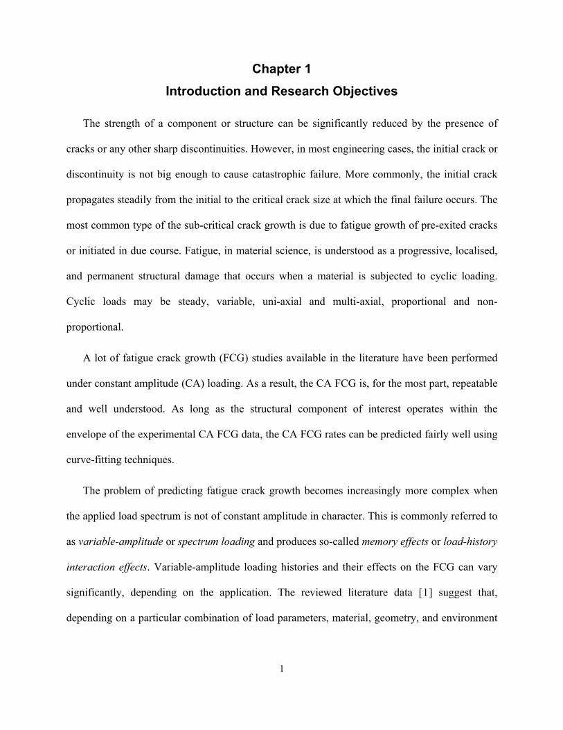
Chapter 1 Introduction and Research Objectives
The strength of a component or structure can be significantly reduced by the presence of
cracks or any other sharp discontinuities. However, in most engineering cases, the initial crack or
discontinuity is not big enough to cause catastrophic failure. More commonly, the initial crack
propagates steadily from the initial to the critical crack size at which the final failure occurs. The
most common type of the sub-critical crack growth is due to fatigue growth of pre-exited cracks
or initiated in due course. Fatigue, in material science, is understood as a progressive, localised,
and permanent structural damage that occurs when a material is subjected to cyclic loading.
Cyclic loads may be steady, variable, uni-axial and multi-axial, proportional and non-
proportional.
A lot of fatigue crack growth (FCG) studies available in the literature have been performed
under constant amplitude (CA) loading. As a result, the CA FCG is, for the most part, repeatable
and well understood. As long as the structural component of interest operates within the
envelope of the experimental CA FCG data, the CA FCG rates can be predicted fairly well using
curve-fitting techniques.
The problem of predicting fatigue crack growth becomes increasingly more complex when
the applied load spectrum is not of constant amplitude in character. This is commonly referred to
as variable-amplitude or spectrum loading and produces so-called memory effects or load-history
interaction effects. Variable-amplitude loading histories and their effects on the FCG can vary
significantly, depending on the application. The reviewed literature data [1] suggest that,
depending on a particular combination of load parameters, material, geometry, and environment

2
similar variable-amplitude load sequences can produce either retardation or acceleration of the
fatigue crack growth.
The goal of the current research is to develop and validate an ’unified fatigue crack growth’
model from the ‘crack initiation stage’ to the ‘final failure’, based on standard (simple smooth
specimens) stress-strain and fatigue material properties. The model has to be applicable to both
constant and variable amplitude loading spectra. More specifically, the following research
objectives were carried out:
• to validate, modify and extend the UniGrow fatigue crack growth model proposed by
Glinka and Noroozi [2]
• to perform analyses in order to improve the understanding of mechanisms controlling
acceleration and retardation phenomena caused by under-loads and overloads
respectively
• to modify the UniGrow fatigue crack growth model and make it applicable to variable
amplitude loading spectra (single and multiple over/under-loads, tensile and
compression stress dominated spectra and arbitrary variable amplitude stress spectra)
• to verify the modified UniGrow fatigue crack growth model by comparing
experimental and predicted fatigue crack growth data obtained under various variable
amplitude loading spectra
In order to accomplish these objectives a set of rules was proposed combining local elastic-
plastic compressive stress fields in the crack tip region generated by a number of successive
stress reversals into one general residual stress field. By using the weight function technique the
effect of the resultant residual stress field can be presented in terms of the instantaneous residual
stress intensity factor and subsequently it can be included into fatigue crack growth driving

3
force. The proposed set of rules allows modeling all effects influencing fatigue crack growth
under arbitrary variable amplitude loading spectrum.
The dissertation is structured in the following way: first the review of existing literature in
the area of constant and variable amplitude fatigue crack growth prediction methodologies with
brief description of their advantages and limitations is presented. The literature review is
followed by detailed description of the UniGrow fatigue crack growth model developed initially
for constant amplitude loading spectra. Since the proposed UniGrow model strongly depends on
the elementary material block size parameter – one of the basic elements of the proposed model,
the next chapter describes methods of its determination. The fifth chapter contains description
and discussion of the original set of “memory rules” followed by qualitative analysis of fatigue
crack growth in the case of variable amplitude loading. The following section shows the fatigue
life predictions and corresponding experimental FCG data obtained under various types of
applied loading spectra. The dissertation is finished with a brief summary, conclusions and
recommendations for future research activities.

4
Chapter 2 Literature Review
2.1 The Linear Elastic Fracture Mechanics
It is generally accepted that the local stresses and strains near the crack tip control the fatigue
crack growth process. Unfortunately, determination of the crack tip stresses and strains in the
case of elastic-plastic behaviour is difficult and it is strongly dependent on the theoretical and
numerical method used for the analysis. Therefore, fracture mechanics principles are often used
in order to defocus the attention from the local crack tip stress-strain field and to express all
necessary quantities in terms of global parameters such as the nominal stress, crack size and
geometry combined into one parameter called the Stress Intensity Factor (SIF).
The groundwork for the development of the brittle fracture hypothesis was laid down around
80 years ago by Griffith [3]. He has shown that the product of the far field stress, the square root
of the crack length, and certain material properties control the crack extension in brittle materials
such as glass. The product was shown to be related to the energy release rate, , which
represents the elastic energy per unit crack of surface area required for a crack extension. Irwin
[
G
4] has made later significant advances by applying Griffith’s theory to metals with small plastic
deformation at the crack tip and using the SIF, K , to quantify the crack tip driving force. By
using Griffith’s energy approach Irwin has shown that the strain energy release rate can be
written as 2KG
E= in plane stress and (1 )
22K
EG υ= − in plane strain, where E is the modulus of
elasticity and ν is Poisson’s ratio.
Consider a through-thickness crack in a linear elastic isotropic body subjected to an external
load (Figure 2-1). An arbitrary stress element in the vicinity of the crack tip with coordinates

5
)( ,r ϕ is also shown in Figure 2-1. Using the mathematical theory of linear elasticity and the
Westergaard [5] stress function in a complex form, the stress field at any point near the crack tip
can be presented in the following form:
( )
( )
( )
3cos 1 sin sin ,2 2 22
3cos 1 sin sin ,2 2 22
3cos sin cos ,2 2 22
x x
y y
xy xy
K rr
K rr
K rr
ϕ ϕ ϕσ ψ ϕπ
ϕ ϕ ϕσ ψ ϕπ
ϕ ϕ ϕτ ψπ
⎡ ⎤⎛ ⎞ ⎛ ⎞ ⎛ ⎞= − +⎜ ⎟ ⎜ ⎟ ⎜ ⎟⎢ ⎥⎝ ⎠ ⎝ ⎠ ⎝ ⎠⎣ ⎦⎡ ⎤⎛ ⎞ ⎛ ⎞ ⎛ ⎞= + +⎜ ⎟ ⎜ ⎟ ⎜ ⎟⎢ ⎥⎝ ⎠ ⎝ ⎠ ⎝ ⎠⎣ ⎦
⎛ ⎞ ⎛ ⎞ ⎛ ⎞= +⎜ ⎟ ⎜ ⎟ ⎜ ⎟⎝ ⎠ ⎝ ⎠ ⎝ ⎠
ϕ
( 2-1)
Higher order terms exist in the solution but they are negligible in the vicinity of the crack tip.
The equations show that the magnitudes of stress components at given point in the crack tip
neighbourhood are entirely dependent on the K factor. All non-zero terms in Eq.2-1 tend to
infinity as the distance to the crack tip, r, tends to zero, and therefore, the exact value of any of
the stress components cannot be determined at the singularity point, i.e. at . 0r =
However, the mathematical model of an ideal sharp crack is, generally speaking, not
physically admissible and the model of a blunt crack with a small but finite crack tip radius
seems to be more realistic. The distribution of stress components ahead of a blunt crack tip with
a tip radius, *ρ , (as shown in Figure 2-2) can be obtained using the Creager and Paris [6]
solution:
* 3 3cos cos 1 sin sin ...2 2 2 2 22 2* 3 3cos cos 1 sin sin ...
2 2 2 2 22 2* 3 3sin sin cos cos ...
2 2 2 2 22 2
x
y
xy
K Krr r
K Krr r
K Krr r
ρ ϕ ϕ ϕ ϕσπ π
ρ ϕ ϕ ϕ ϕσπ π
ρ ϕ ϕ ϕ ϕτπ π
⎡ ⎤= − + − +⎢ ⎥⎣ ⎦⎡ ⎤= + +⎢⎣ ⎦
= − + +
+⎥ ( 2-2)

6
According to Figure 2-2 the crack tip position is located at *
2r ρ
= , thus all stress components at the
crack tip are finite.
2.2 Constant Amplitude Fatigue Crack Growth Models
As mentioned in previous section, the SIF controls the local material behaviour in the crack tip
region; however, the significance of this parameter can be fully understood only when linear elastic
fracture mechanics is incorporated into fatigue analyses.
It was found by Paris [7] that fatigue crack growth rate can be related to the applied cycling loading
and the geometry of the cracked body by using appropriate SIF solution. Since that time, the fatigue crack
growth rate, , data are most frequently presented as a function of the applied stress intensity
range,
/da dN
applKΔ , as shown in Figure 2-3. The applied stress intensity range, applKΔ , is a function of the
applied stress range applσΔ .
max, min,appl appl appl applK K K aσ πΔ = − = Δ Y ( 2-3)
Fatigue crack growth curve is traditionally divided into three stages as shown in Figure 2-3.
1. Threshold regime: the crack size is of the order of micro-structural dimensions of the
material and/or of the same order as the crack tip plastic zone size. Fatigue crack growth in
this regime is highly dependent on the material microstructure and cracks usually grow in
the direction of maximum shear stress. This regime is the most important in the mechanical
engineering design and fatigue durability assessments of cracked objects.
2. The Paris regime: the crack size is large in comparison with material microstructural
dimensions. Fatigue crack growth in this regime does not depend on material micro-
structural features and the direction of the crack growth is perpendicular to the maximum
7
principal stress. This regime is important for setting up inspection programs required for
structural safety.
3. The static failure regime: the crack size or the plastic zone size may be of the same order as
the smallest structural dimension. This regime contributes to fatigue life predictions by
determining conditions for fracture. The contribution of this regime to the fatigue life of a
structure is relatively small due to high fatigue crack growth rate.
Based on experimental observations many researchers have concluded that fatigue crack growth
depends not only on the applied stress intensity range but also on the ratio between the maximum and
minimum applied stress intensity factor, min,
max,
appl
appl
KR
K= . In other words, even under the same stress
intensity range ΔK the fatigue crack growth varies with varying stress ratio R.
Next is the discussion of various fatigue crack growth models.
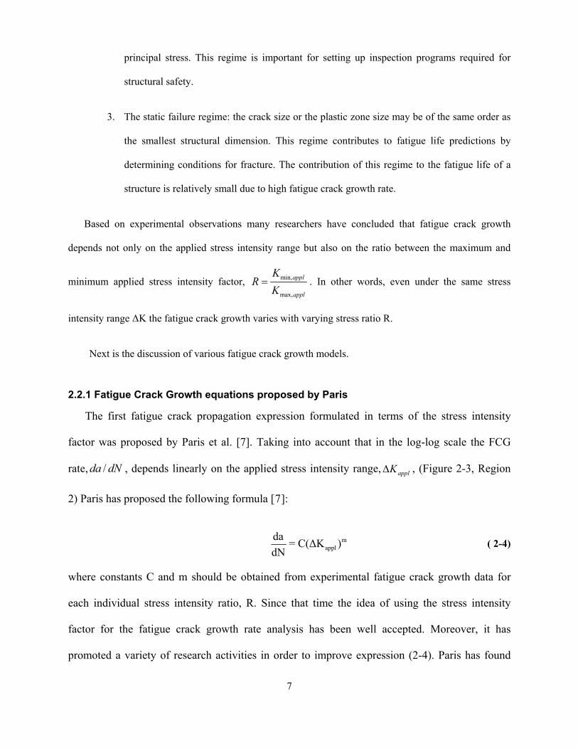
2.2.1 Fatigue Crack Growth equations proposed by Paris
The first fatigue crack propagation expression formulated in terms of the stress intensity
factor was proposed by Paris et al. [7]. Taking into account that in the log-log scale the FCG
rate, , depends linearly on the applied stress intensity range,/da dN applKΔ , (Figure 2-3, Region
2) Paris has proposed the following formula [7]:
mappl
da = C(ΔK )dN
( 2-4)
where constants C and m should be obtained from experimental fatigue crack growth data for
each individual stress intensity ratio, R. Since that time the idea of using the stress intensity
factor for the fatigue crack growth rate analysis has been well accepted. Moreover, it has
promoted a variety of research activities in order to improve expression (2-4). Paris has found

8
that the exponent made it possible to simulate da/dN-ΔK trends for a variety of metallic
materials. The typical value of m in Eq. 2-4 varies usually from 2 to 4. Again, there is typically a
unique combination of C and m for each combination of environment, temperature, and the stress
ratio. In spite of the fact that Eq. 2-4 requires knowledge of a large amount of fatigue crack
growth constants even for one material, it is still frequently used in engineering practice.
4m =
2.2.2 Two-parameter models
Since Paris’ original work, many variations of the power law equation have been postulated
to better fit various regimes of the FCG rate curve and/or to take into account the stress ratio
dependence. Forman et al.[8] have proposed a relationship that captures two aspects of the
fatigue crack growth curve, i.e. the stress ratio effect on the FCG rate and the rapid increase of
FCG rate in Region 3 (Figure 2-3).
( )
( )1
m
appl
C appl
C KdadN R K K
Δ=
− − Δ ( 2-5)
where KC is the fracture toughness and and m are constants required to fit the FCG data into
one da/dN-ΔK curve. However, as it has been mentioned already, Region 3 of the FCG curve is
not very important from the fatigue crack propagation point of view, since the fatigue life of a
component is very short when the SIF approaches the fracture toughness.
C
In order to verify the validity of any fatigue crack growth model for constant amplitude
loading spectra, several experimental fatigue crack growth curves with different mean stresses
(or R ratios) have to be presented in terms of appropriate driving force. The correct model should
collapse all the experimental data points into one ‘master’ curve indicating that the mean stress
effect is accounted for. Figure 2-4 shows the experimental FCG data for AL 7075 T6 material
obtained at six different stress ratios R.

9
In order to check the validity of the Forman FCG expression (Eq. (2-5)) one has to calculate
the new parameter ( )1 C appldaQ R K KdN
⎡= − − Δ⎣ ⎤⎦ and plot it in terms of the applied stress
intensity range, . The results shown in Figure 2-5 indicate that Eq. 2-5 is capable to
account for the mean stress effect. The model requires the prior knowledge of parameter, KC.
Parameters, C and m, need to be found by fitting eq.(2-5) into a set of experimental constant
amplitude FCG data.
applKΔ
Numerous researchers [9-15] have attempted, during the last four decades, to modify the
Paris equation by introducing a two-parameter driving force by combining the maximum stress
intensity factor and the stress intensity range.
Broek, Schijve, and Erdogan [9] proposed in 1963 the following form of two-parameter
driving force which allows to account for the mean stress effect in Region 2 (Figure 2-3).
2max
da CK KdN
= Δ ( 2-6)
Another empirical relationship between applied loading parameters and fatigue crack growth
rate was proposed by Weertman [10].
4
2 2maxC
da C KdN K K
Δ=
− ( 2-7)
Similarly to the approach used in Forman’s model one can define analogous parameter
2 2maxC
daQ K KdN
⎡= −⎣ ⎤⎦ in the Weertman equation and present it in terms of the applied stress
intensity range. A set of FCG data for the AL 7075 T6 alloy is shown in this format in Figure
2-6. Unfortunately, Eq. 2-7 was not capable to collapse the all experimental FCG data into one

10
‘master’ curve. The Weertman model requires the knowledge of the fracture toughness, KC, but
only one parameter, C, has to be fitted into the reference CA FCG data.
Priddle [11] proposed the equation which can describe the fatigue crack growth rate curve in
over all regimes by taking into account both the fracture toughness and the threshold stress
intensity range. As one can see, the proposed form (Eq. 2-8) is based on two assumptions: first,
the fatigue crack growth rate has to tend to 0 while the applied stress intensity range approaches
the threshold and, second, the fatigue crack growth should tend to infinity when the maximum
applied stress intensity factor approaches the fracture toughness.
max
m
th
IC
K Kda CdN K K
⎛ ⎞Δ − Δ= ⎜ −⎝ ⎠
⎟ ( 2-8)
The same experimental FCG data for the AL 7075 T6 alloy in terms of Priddle’s fatigue
crack driving force is shown in Figure 2-7. All experimental points collapsed relatively well onto
one ‘master’ curve in Paris (second) FCG Regime, however some deviations exist in the first and
third FCG regimes. The model requires the knowledge of two material constants, ΔKth and KC,
and two additional constants have to be obtained from experimental CA FCG data.
Another empirical law based on the same logic and enabling to fit the entire fatigue crack
growth curve was developed by McEvily [12] in the form of:
( )2
max
1thIC
da KC K KdN K K
⎛ ⎞Δ= Δ − Δ +⎜ ⎟−⎝ ⎠
( 2-9)
The experimental FCG data in terms of Mc Evily’s fatigue crack driving force (Figure 2-8) is
very similar to that one based on Eq. 2-8, however the spread of the experimental FCG data is
wider. Similar to Priddle’s model, Eq. 2-9 requires the knowledge of ΔKth and KC, however only
on parameter has to be fitted from the CA FCG data.

11
One of the first empirical and relatively successful fatigue crack growth models accounting
for the R-ratio effect was proposed by Walker [13].
1max,
p pappl appl
da C K KdN
γ−⎡ ⎤= Δ⎣ ⎦ (2-10)
A similar expression was proposed later by Donald and Paris [14]. In both cases expression
(2-10) is capable to correlate the fatigue crack growth rates obtained at a variety of ratios R It has
been shown (Figure 2-9) that by empirical fitting of parameters ‘p’ and ‘γ’ it is possible to
correlate fatigue crack growth data for stress ratios in the range of 2 R < 1− ≤ . The model is
based on three parameters which has to be fitted using experimental FCG data for CA loading.
A two parameter driving force involving the maximum stress intensity factor, , and
the stress intensity range, , was also suggested by Sadananda and Vasudevan [
max,applK
applΔK 15]. They
have also postulated the existence of two thresholds, i.e. the maximum threshold stress intensity
factor, , and the threshold stress intensity range,max,thK thKΔ . Both should simultaneously be
exceeded to make the fatigue crack growing.
2.2.3 The crack closure model
A very popular and often controversial approach to account for the stress ratio dependence
has been the incorporation of the crack tip closure-corrected stress intensity range, effKΔ .
In its simplest form, the applied stress intensity range applKΔ in Eq. 2-4 is replaced by the
effective stress intensity range maxeff opK K KΔ = − where opK is the stress intensity level at which
the crack tip becomes fully open as proposed by Elber [16]. The effective stress intensity range
is used to explain the mean stress effect on fatigue crack growth rates. However, at high stress

12
ratios where the crack tip closure is insignificant and the applied stress intensity range is almost
equal to effective one the crack tip closure model cannot account for the mean stress effect on
the fatigue crack growth.
It has been recognized by researchers that plasticity induced crack closure is not the only
mechanism responsible for the crack closure effect. Suresh and Ritchie [17] have proposed five
different crack closure mechanisms in order to explain crack tip closure effects and the near
threshold fatigue crack behaviour in particular. These are the crack tip closure induced by the
Plasticity, crack surface Roughness or asperity, Oxidation, Phase transformation and Viscous
fluids trapped behind the crack tip.
In spite of large amount of data generated during the last thirty years it is still difficult to
correlate crack closure measurements with the crack growth behaviour. Experimental
observations show that the crack opening load level depends on the measurement location
relative to the crack tip and the measurement technique [18]. Ling and Schijve [19] have also
found that heat treatment can change the crack opening load.
Garret and Knott [20] have shown that the crack closure phenomenon had little effect on
fatigue crack growth in plane strain conditions. Moreover, the crack tip crack closure cannot be
used in order to explain fatigue crack growth delays induced by overloads in plane strain
conditions at high stress ratios. The finite element data produced by Wei and James [21]
confirmed that the crack opening load depends also on the stress state in the vicinity of the crack
tip.
Based on observations of the fatigue crack growth on the stress-ratio dependence in threshold
regime in vacuum studied on both steel and aluminium alloys, Louat [22] et al. concluded the

13
following“… closure cannot be expected to provide a rationale for many fatigue crack growth
phenomena, such as load-ratio effects on thresholds.”
However, despite of these difficulties the crack closure model stays at present as one of the
most popular tools for fatigue crack growth analyses.
2.3 Variable Amplitude Fatigue Crack Growth Models
In this part the fatigue crack growth behaviour observed in fatigue tests performed under
variable amplitude loading is to be reviewed. It can be concluded in general that depending on
particular combination of applied loading parameters, material properties, specimen geometries,
microstructure, and environmental conditions the same variable amplitude loading sequence can
produce either acceleration or retardation of fatigue crack growth. The description of the most
popular variable amplitude fatigue crack growth models can be found in the book by Stephens et
al. [23]
The main physical arguments that have been used in order to explain the load-interaction
effects on fatigue crack growth can be listed chronologically as follows:
• Crack tip blunting
• Cyclic plasticity induced residual stress around the crack tip
• Crack tip plasticity
• Plasticity induced crack closure.
2.3.1 The Crack tip blunting
The main idea proposed first by Christensen [24] assumes that a crack blunted by an
overload behaves as a notch. In such a case, the retardation of fatigue crack growth is manifested
by the number of cycles required to reinitiate and propagate the crack from the notch.

14
Experimental investigations were carried out [25-26] in order to prove or disprove this
assumption. Based on the fatigue crack growth observations it has been found [25] that by stress
reliving the cracked specimen immediately after application of a single overload the usual
retardation effect almost disappeared except after application of very high overload ratios.
Another group of researches has observed [26] that both the retardation of the FCG after a single
overload and the acceleration after a single under-load were accompanied by crack tip blunting.
As a result of these observations the crack tip blunting is often considered as a mechanism
which prevents crack from closing during the unloading reversal following a high overload.. It
is also believed that crack tip blunting is responsible for a shortly lasting acceleration of fatigue
crack immediately after the application of the overload.
2.3.2 Residual stresses
The residual stress concept is based on the fact that during the unloading reversal following
an overload compressive residual stresses can be generated in the small region around the crack
tip[27]. Analytical investigations and experimental measurements show [28] that the spread of
the compressive stress zone strongly depends on the applied loading and it is always larger after
the overload than during the application of preceding load cycles. According to Schijve [27] the
superposition of compressive residual and applied stresses gives the resultant effective stresses
responsible for temporary retardation of the fatigue crack growth within the compressive residual
stress zone. According to the residual stress concept the acceleration of the fatigue crack growth
after an under-load is due to tensile stresses induced ahead of the crack tip.
Since the proposed UniGrow fatigue crack growth model is based on the analysis of local
elastic-plastic strains and stresses near the crack tip and is accounting for compressive stresses
induced due to reversed plastic deformations it can be classified as the ‘Residual Stress’ model.

15
2.3.3 The Crack tip plasticity
The most popular crack tip plasticity models were proposed by Wheeler [29] and Willenborg
[30] in the early 70s. Both models can predict fatigue crack growth retardation fairly well as long
as the crack propagates through the overload plastic zone. According to Wheeler, fatigue crack
growth after an application of a single overload can be determined using the modified Paris
equation:
( ) ( )mp ii
i
da C C KdN
⎡ ⎤= Δ⎣ ⎦ ( 2-11)
where, the retardation parameter, pC , depends on the current plastic zone size, ,p ir , and the
overload plastic zone size, ,p ovr . Index ‘i’ refers to the particular loading cycle in a loading
history.
( ) ,
,
p
p ip i
p ov i
rC
r a⎛ ⎞
= ⎜⎜ − Δ⎝ ⎠⎟⎟ ( 2-12)
The exponent, p, is a fitting empirical parameter which depends on the loading history.
The main disadvantage of that model is the shaping factor, p, which has to be experimentally
determined for each individual loading history. Additionally, the so called delayed fatigue crack
growth retardation phenomenon and fatigue crack growth acceleration caused by under-loads
cannot be simulated by the Wheeler model.
The Willenborg model states that crack growth retardation is caused by compressive stresses
in the crack tip region induced by an overload. The crack growth retardation after an overload is
accounted for by substituting the effective stress ratio, Reff, and the effective stress range, Δσeff,
into the Forman Eq. 2-5. No additional parameters are necessary.

16
According to the model, so-called boundary stress intensity factor, Kb, has to be calculated
based on the λ parameter shown in (Figure 2-10).
( )( )b ys o p ysOVK a r aσ γπ σ γπλ= + − = ( 2-13)
Where, ysσ is the yield stress, γ is the over-load ratio (OLR), is the crack length at the
moment of the over-load application,
oa
( )p OVr is the plastic zone size induced by the overload
(Figure 2-10). The residual stress intensity factor, Kres, and effective stress intensity factor, Keff,
are then calculated as:
maxres bK K K= − ( 2-14)
eff appl resK K K= − ( 2-15)
However, Ouk [31] has shown that when sufficiently high overload ratio is applied both the
maximum and minimum effective SIF can go below zero, the Willenborg model predicts
complete crack arrest in such a case, which may not actually happen in reality
In addition, the Willenborg model cannot predict the delayed retardation effect or in other
words, the maximum crack growth retardation occurs immediately after application of the
overload. Moreover, similar to Wheeler model, the fatigue crack growth acceleration cannot be
predicted by the Willenborg model due to the fact that only tensile loads are counted and
compressive loads are neglected [23]. Nevertheless, the major advantage of the Willenborg
model is that only constant amplitude fatigue crack growth data is required for the analysis of
fatigue crack growth under variable amplitude loading histories.

17
2.3.4 The Plasticity induced crack closure
A very popular approach to account for load – interaction effects is the incorporation of the
effective stress intensity range, effKΔ , corrected for the closure effect. The crack tip closure
model proposed initially by Elber [16] was later modified to model the fatigue crack growth
under variable amplitude loading. Numerous studies have been carried out to explain various
fatigue crack growth phenomena using the crack tip closure concept. Detailed descriptions of
these models can be found in reference [32]. The most successful, among them, is the finite
element method based model proposed by Newman [33].The model is based on the analysis of
the strip yield plastic zone that is left in the wake of the advancing crack. According to the
Newman model the plastically deformed material can induce crack closure even at positive stress
levels. Since the amount of crack closure differs for each level of the applied stress or loading the
fatigue crack growth rate should be calculated on a cycle by cycle basis. Therefore, the
determination of the crack opening load level, Pop, and the corresponding effective stress
intensity range, Keff, becomes the main element in the crack closure model when applied to
variable amplitude loading histories.
Newman has assumed [33] that the crack opening load, Pop, remains constant during a small
crack increment and does not change after each loading cycle. For simplicity, it is assumed in
engineering applications, that the crack opening load, Pop, and corresponding crack opening
stress intensity factor, Kop, are constant for a given block of variable amplitude loading. In such a
case the crack opening load, Kop, can be estimated from the constant amplitude fatigue crack
growth test data with the equivalent stress intensity range defined as ,
where and are the maximum and minimum stress intensity factors respectively in
the block of variable amplitude loading [
max, min,VA VAK K KΔ = −
max,VAK min,VAK
34]. However, the fatigue crack growth rate is predicted
for each cycle using the Paris law (Eq. 2-4).

18
( ,
m
eff ii
da A KdN
= Δ ) ( 2-16)
where: , max,eff i i opK K KΔ = − . The constant ‘A’ is not the same as the constant ‘C’ in the Paris
equation. It should be estimated based on the effective stress intensity range, ΔKeff. Constants
‘A’ and ‘C’ can be correlated using the following equation [35].
( )m
i
CAU
= ( 2-17)
where ,
,
eff ii
appl i
KU
KΔ
=Δ
.
Equation (2-17) should be solved for ‘N’ using a numerical integration method in order to
obtain cycle by cycle fatigue crack growth increments from an initial to the final crack size. A
number of computer programs, such as NASGRO, FASTRAN-2, MODGRO, and FLAGRO
have been developed to estimate fatigue life under variable amplitude loading based on the
fatigue crack tip closure approach.

19
Figure 2-1: Sharp crack in a linear elastic domain
Figure 2-2: Blunted crack in a linear elastic domain
S
S
ρ*
a ρ*/2
yσ
y
S
x
τxy
σy
σx
2yKσ =
ϕ
xπ
r a
S
SS
y
x

20
ΔKth
m
Region 2
Region 3
Region 1
Kmax= KIc Figure 2-3: General Shape of the Fatigue Crack Growth Rate curve
da/dN vs. ΔK; Al 7075-T6 (data of Newman [70] and Jiang[71])
1.E-12
1.E-11
1.E-10
1.E-09
1.E-08
1.E-07
1.E-06
1.E-05
1.E-04
1.E-03
1 10 100ΔΚapl, [MPa√m].
da/d
N, [
m/c
yc].
R=0.82..0.7R=0.5R=0.33R=0R=-1R=-2
Original FCG Data for the Al 7075 T6 alloy
Figure 2-4: Experimental FCG data for Al 7075 T6 alloy [71, 73]

21
Figure 2-5: FCG data for AL 7075 T6 alloy in terms of Forman’s driving force Eq. 2-5
Figure 2-6: FCG data for AL 7075 T6 alloy in terms of Weertman’s driving force Eq. 2-7

22
Figure 2-7: FCG data for AL 7075 T6 alloy in terms of Priddle’s driving force Eq. 2-8
Figure 2-8: FCG data for AL 7075 T6 alloy in terms of Mc Evily’s driving force Eq. 2-9

23
Figure 2-9: FCG data for AL 7075 T6 alloy in terms of Walker’s driving force Eq. 2-10
Figure 2-10: Schematic of the Willenborg model
Plastic zone of OL
Plastic zone of cycle ‘i’
Plastic zone required to eliminate the effect of OL
Crack length at application of OL
a
a0
rp
(rλ
p)ol

24
Chapter 3 The Two-Parameter Total Driving Force Model
3.1 Introduction and basic assumptions
In order to overcome the difficulties in existing FCG models described in Chapter 2, the Two
–Parameter Total Driving Force has been proposed earlier by Noroozi and Glinka [2]. The model
is based on an actual elastic-plastic material response in the crack tip region. The following
assumptions concerning the material microstructure, crack geometry, and material properties
were applied.
• The material is assumed to be composed of identical elementary material blocks of a
finite dimension *ρ .
• The fatigue crack can be analyzed as a sharp notch with a finite tip radius of
dimension *ρ .
• The material cyclic and fatigue properties used in the proposed model are obtained from
the Ramberg-Osgood (Eq. 3-1) cyclic stress strain curve [36]
'
1n
'
σ σε = +E K
⎛ ⎞⎜ ⎟⎝ ⎠
(3-1)
and the strain-life (Manson-Coffin) fatigue curve [37] of (Eq. 3-2).
( ) ( )b cff
σΔε = 2N + ε 2N2 E
′′ (3-2)
• The number of cycles ‘N’ required to fail the first elementary material block at the crack
tip can be determined from the strain-life (Manson-Coffin) fatigue curve (Eq. 3-2) by
accounting for the stress-strain history at the crack tip and by using the Smith-Watson-
Topper (SWT) fatigue damage [38] parameter of (Eq. 3-3).

25
maxΔεD = σ2
( 3-3)
• The fatigue crack growth rate can be determined as the average fatigue crack propagation
rate over the elementary material block of the size ‘ρ*’.
f
da ρ*dN N
= ( 3-4)
The verification of the model has been carried out by Noroozi and Glinka [2, 39] for the case
of constant amplitude loading. The detailed description of the model verification based on a large
amount of constant amplitude FCG data was presented by Noroozi [39]. Brief description of the
Two – Parameter Total Driving Force model is presented below.
3.2 Residual compressive stresses at the crack tip, the residual stress intensity factor, and the total stress intensity parameters
According to the model, the knowledge of the local elastic-plastic stresses and strains in the
crack tip region is required for the analysis. The calculation of elastic-plastic strains and stresses
at the crack tip requires solving the elastic-plastic stress-strain boundary problem of a cracked
body. Analytical solutions of such complex problems are seldom attainable. Numerical Finite
Element (FE) solutions are feasible but not very convenient in practice due to the complexity of
the FE model and the lengthy calculations in the case of cyclic loading. Therefore simplified
methods based on the Neuber [40] or the ESED rule [41] have been chosen for the elastic-plastic
stress/strain analysis. The methods require two step approach, i.e. first the linear elastic stress-
strain analysis needs to be carried out and, in the second step, the actual elastic-plastic crack tip
strains and stresses are determined from the Neuber or the ESED rule for which the linear elastic
stress data is the input. Both rules have the same complexity level and either of them can be

26
used; however, due to the fact that the Neuber rule is more conservative it is preferable in
practice.
3.2.1 Linear Elastic analysis of stresses and strains ahead of the crack tip
The Neuber rule requires the knowledge of the local elastic stresses and strains in the crack
tip region obtained for the actual crack and component geometry and the applied loading.
However, there are some difficulties in defining the crack tip geometry within the mechanics of
continuum framework. The classical fracture mechanics solutions (described in Section 2.1)
concerning stresses and strains at the crack tip were derived for a sharp crack having the tip
radius 0* =ρ . Such crack tip geometry leads to the singular solution resulting in unrealistically
high strains and stresses in the vicinity of the crack tip. In spite of the importance of these
fundamental fracture mechanics solutions they unfortunately cannot be directly used for the
determination of the actual stresses and strains in the vicinity of the crack tip. Therefore, several
attempts were made in the past [42] to model the fatigue crack as a notch with a small but finite
tip radius *ρ > 0, as shown in Figure 3-1.
The advantage of using the blunt crack model lies in the fact that the notch theories can be
applied and the calculated crack tip stresses and strains become more realistic. There are two
important implications resulting from such a model: first the crack tip radius is assumed to be
finite ( > 0) and secondly the crack region just behind the tip remains open even if high
compressive load is applied. The methodology for estimating was described by Noorozi in
reference [
*ρ
*ρ
39]; however the accuracy of the proposed methodology strongly depends on the
accuracy of the near threshold fatigue crack growth experimental data (which is usually not the
most accurate itself). Therefore, additional modifications were proposed and implemented by the
author in order to improve the methodology and they are discussed in the next chapter.
27
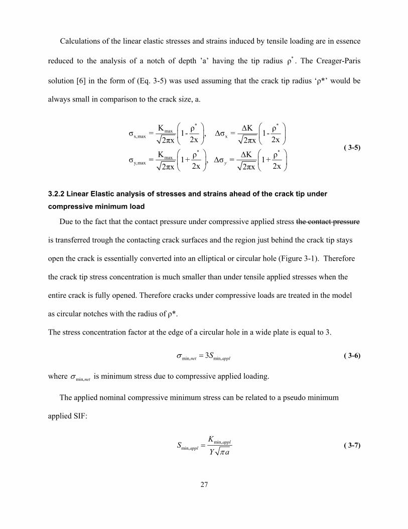
Calculations of the linear elastic stresses and strains induced by tensile loading are in essence
reduced to the analysis of a notch of depth ’a’ having the tip radius . The Creager-Paris
solution [
*ρ
6] in the form of (Eq. 3-5) was used assuming that the crack tip radius ‘ρ*’ would be
always small in comparison to the crack size, a.
* *max
x,max x
*max
y,max
K ρ K ρσ = 1- , σ = 1-2x 2x2πx 2πx
K ρ K ρσ = 1+ , σ = 1+2x 2x2πx 2πxy
⎛ ⎞ ⎛ ⎞ΔΔ⎜ ⎟ ⎜ ⎟
⎝ ⎠ ⎝ ⎠⎛ ⎞ ⎛ ⎞Δ
Δ⎜ ⎟ ⎜ ⎟⎝ ⎠ ⎝ ⎠
* ( 3-5)
3.2.2 Linear Elastic analysis of stresses and strains ahead of the crack tip under compressive minimum load
Due to the fact that the contact pressure under compressive applied stress the contact pressure
is transferred trough the contacting crack surfaces and the region just behind the crack tip stays
open the crack is essentially converted into an elliptical or circular hole (Figure 3-1). Therefore
the crack tip stress concentration is much smaller than under tensile applied stresses when the
entire crack is fully opened. Therefore cracks under compressive loads are treated in the model
as circular notches with the radius of ρ*.
The stress concentration factor at the edge of a circular hole in a wide plate is equal to 3.
min, min,3net applSσ = ( 3-6)
where min,netσ is minimum stress due to compressive applied loading.
The applied nominal compressive minimum stress can be related to a pseudo minimum
applied SIF:
min,min,
applappl
KS
Y aπ= ( 3-7)

28
Therefore, the minimum compressive stress at the circular hole representing the crack under
compression can be finally related to the minimum applied SIF.
min,min,
3 applnet
KY a
σπ
= ( 3-8)
However, the Creager-Paris solution suggests that if the problem is treated as a blunt crack a
certain stress intensity factor, Kmin,net, needs to be applied to generate the same stresses σmin,net as
above.
min,min,
2*net
net
Kσ
πρ= ( 3-9)
By combining Eq. 3-8 and Eq. 3-9 the following expression for Kmin,net can be derived:
min, min,3 *2net applK KY a
ρ= . ( 3-10)
Thus the range of the stress intensity factor under tension-compression loading is determined as:
max, min, max, min,3 *2net appl net appl applK K K K KY a
ρΔ = − = −
In order to determine the fluctuations of the linear elastic stress near the crack tip, it is necessary
to account for the difference in the tensile and compressive part of the cycle. It can be done by
replacing the minimum applied SIF with the minimum net SIF in Eq. 3-5.
*
max,appl min,3 * 1 ρσ = K 1+
2x2 2πxnet applKY a
ρ⎛ ⎞ ⎛ ⎞Δ −⎜ ⎟ ⎜ ⎟⎜ ⎟ ⎝ ⎠⎝ ⎠
( 3-11)
It can be seen from Eq. 3-11 that the contribution of the compressive part of a loading cycle to
the local elastic stress range is relatively small and depends on the crack tip radius ρ*, and the
crack size, a.

29
3.2.3 Elastic-plastic stresses and strains ahead of the crack tip
The purpose of the elastic-plastic stress-strain analysis is to determine the actual stress-strain
history and the residual stress induced by reversed plastic yielding in the crack tip region. In
order to avoid solving the complete but unfortunately very complex elastic-plastic cracked body
boundary problem for each load/stress reversal, the well known Neuber rule [40] was used. The
Neuber rule was originally derived for a uni-axial stress state (i.e. pure shear) but it has been
later expanded [43,44] for multi-axial proportional and non-proportional loading histories. The
Neuber rule states the equivalence of the strain energy at the notch tip between the linear elastic
and elastic-plastic behaviour of geometrically identical notched bodies subjected to identical
external loading systems. Zeng and Fatemi [45] made the comparison between stresses and
strains obtained using finite element analysis and the Neuber rule for notched flat plates with
different stress concentration factors. Based on this results, it can be concluded that the Neuber
rule provides stresses and strains close to ones obtained using the finite element analysis as long
as the applied nominal stress is less than 0.8*Sys. Additionally, according to reference [1] the
Neuber rule in general gives stresses and strains close to ones obtained from experiments or
more conservative if the applied nominal stress is high.
In the case of an uni-axial stress state at the notch tip the Neuber rule provides the
relationship (Eq. 3-12) between the hypothetical linear elastic notch tip stress-strain input data
and the actual elastic-plastic stress-strain response at the notch tip.
( 3-12) e e a ay y y yσ ε = σ ε
The idea of the Neuber rule in uni-axial case is schematically illustrated in Figure 3-2.
For cracked bodies in plane stress the stress state near the crack tip is bi-axial. In the case of
bodies in plane strain conditions the near tip stress state is tri-axial but the third principal stress is

30
a function of the other two stress components and in both situations the modified bi-axial Neuber
rule can be used. In addition, the elastic stress tensor used as the input does not rotate and all
stress components change proportionally. Therefore, the Hencky equations [46] of the total
deformation theory of plasticity can be applied.
In the case of bi-axial stress state the combination of the Hencky stress-strain relationships,
the Ramberg-Osgood stress-strain constitutive equation (3-1) and the multiaxial Neuber rule [43]
leads to the set of four equations (Eq. 3-13) from which all maximum elastic-plastic crack tip
strains and stresses can be determined:
( )
( )
aeqa a a a a
x,max x,max y,max x,max y,maxaeq
aeqa a a a a
y,max y,max x,max y,max x,maxaeq
e e a ax,max x,max x,max x,max
e e a ay,max y,max y,max y,max
f(σ )1 1ε = σ - νσ + σ - σE σ 2
f(σ )1 1ε = σ - νσ + σ - σE σ 2
σ ε = σ ε
σ ε = σ ε
⎧ ⎛ ⎞⎪ ⎜ ⎟
⎝ ⎠⎪⎪
⎛ ⎞⎪⎜⎨⎝⎪
⎪⎪⎪⎩
⎟⎠
)
( 3-13)
where: ( ) (2 2a a a a aeq x,max x,max y,max y,maxσ = σ -σ σ + σ and
1a neqa
eq
σf(σ ) =
K
′⎛ ⎞⎜ ⎟⎜ ⎟′⎝ ⎠
.
Actual elastic-plastic stress and strain ranges can be determined from similar set of equations.
( )
( )
aeqa a a a
x x y xaeq
aeqa a a a
y y x yaeq
e e a ax x x xe e a ay y y y
f(σ )1 1ε = σ - ν σ + σ - σE σ 2
f(σ )1 1ε = σ - ν σ + σ - σE σ 2
σ ε = σ ε
σ ε = σ ε
⎧ ⎛ ⎞Δ Δ Δ Δ Δ⎪ ⎜ ⎟⎝ ⎠⎪
⎪⎛ ⎞⎪Δ Δ Δ Δ Δ⎨ ⎜ ⎟⎝ ⎠⎪
⎪Δ Δ Δ Δ⎪⎪Δ Δ Δ Δ⎩
ay
ax
( 3-14)
where: ( ) ( )2 2a a a aeq x x y yσ = σ - σ σ + σΔ Δ Δ Δ a and
1a neqa
eq
σ1f(σ ) =2 2K
′⎛ ⎞⎜ ⎟⎜ ⎟′⎝ ⎠
.

31
y
Based on Eq. 3-13 and Eq. 3-14 the residual stresses (i.e. stresses remaining in the material after
an application of a loading cycle) can be calculated from equation 3-15.
,maxa a
r yσ σ σ= − Δ
( 3-15)
In order to determine the residual stress distribution ahead of the crack tip the procedure
described above needs to be repeated for a sufficient number of points in the crack tip region.
The elastic-plastic stress-strain analysis discussed in this section assumes Massing type
material behavior which is common for steel and aluminum alloys. However, if the material is a
non-Massing type, another appropriate stress-strain model has to be chosen and implemented in
order to determine local elastic-plastic stresses and strains in the crack tip region.
3.3 Residual compressive stresses near the crack tip
After calculating the elastic-plastic strains and stresses at various locations ahead of the crack
tip, it may happen that the stress field ahead of the crack tip induced by the application of
subsequent loading and unloading reversal is compressive. Schematic diagrams showing stress
distributions ahead of the crack tip corresponding to the maximum and minimum load level
respectively generated at two different stress ratios R are shown in Figure 3-3.
Both stress distributions, i.e. those corresponding to the maximum and minimum load and
high applied stress ratios (Rappl>0.5) are most often tensile. In such a case the crack tip
displacement field and the crack tip stress field are dependent only on the applied stress intensity
factor. However, compressive stresses might be generated at the minimum load level in the case
of low stress ratios (Rappl < 0.5). These compressive stresses remain present in the crack tip
region even at the zero applied load level. Therefore these compressive stresses have to be
included into the mathematical expression combining the applied load, the elastic-plastic crack
tip stress-strain response and the displacement field. The compressive stress effect needs to be

32
expressed in terms of the stress intensity factor before it can be included into any fatigue crack
growth expression.
3.3.1 Calculation of the residual stress intensity factor, rK
The compressive stress ahead of the crack tip prevents deformation and opening behind the
crack tip. Therefore it was assumed, analogously to the well known Dugdale model, that the
effect of compressive stresses σr(x) can be quantified in terms of the stress intensity factor.
Calculation of the residual stress intensity factor was carried out using the weight function
method [47,48]. The universal one dimensional [49] weight function (Eq. 3-16) was used in the
analysis.
1 312 2
1 2 32P x x xm(x,a) = 1+ M 1- + M 1- + M 1-
a a2π(a - x) a
⎡ ⎤⎛ ⎞ ⎛ ⎞ ⎛ ⎞⎢ ⎥⎜ ⎟ ⎜ ⎟ ⎜ ⎟⎢ ⎥⎝ ⎠ ⎝ ⎠ ⎝ ⎠
⎣ ⎦
( 3-16)
M1, M2 and M3 factors for various geometrical configurations are given in reference [49].
The stress intensity factor is calculated by integrating the product of the compressive residual
stress field σr(x) and the weight function over the crack length. m(x,a)
( 3-17) a
r r0
K = σ (x)m(x,a)dx∫
A special numerical procedure was developed [50] for calculating the integral (3-17). It has been
also found that by using a piece-wise linear approximation of the residual stress field the integral
(3-17) can be written as a closed form mathematical expression.
Typical residual stress distribution for a crack in Al 7075 T6 alloy obtained using stress
intensity factors ΔKappl=Kmax,appl=10 MPa√m and the Neuber rule (Eq. 3-13 and Eq. 3-14) is
shown in Figure 3-4.
33
It can also be shown that geometrical terms 1 312 2
1 2 3x xM 1- , M 1- , and M 1-a a
⎛ ⎞ ⎛ ⎞ ⎛ ⎞⎜ ⎟ ⎜ ⎟ ⎜ ⎟⎝ ⎠ ⎝ ⎠ ⎝ ⎠
xa
in
the weight function (Eq. 3-16) are not important as long as the extend of the integration region x0
(i.e. the width of the residual compressive zone) is relatively small in comparison with the crack
size ‘a’. This observation led to the idea of eliminating those terms from Eq. 3-16 and making it
geometrically independent. Therefore, the universal geometrically independent one-dimensional
weight function applicable to the crack tip region has been used in the following form:
12Pm (x,a) =
2π(a - x) (3-10 b)
For the loading distribution shown in Figure 3-4 the difference between residual SIFs obtained
using the original weight function (Eq. 3-16) and the simplified one (Eq. 3-16 b) was only
around 0.02%.
It has been shown that as long as crack size is less than 80% of the specimen width and the
region of integration is smaller than half of the crack size (x0 < 0.5a) the relative error is always
less than 032
xa
. Therefore, the simplified weight function can be used for crack/specimen
geometries even where the exact solution is not known.
3.3.2 The Total maximum stress intensity factor and total stress intensity range
Before the applied maximum stress intensity factor, Kmax,appl, and the stress intensity range
,ΔKappl, are fully effective they have to overcome the effect of residual compressive stresses
quantified in terms of the residual stress intensity factor Kr. Therefore the applied stress intensity
range, applKΔ , and the maximum SIF, , representing the applied load and crack
geometry, have to be somehow combined with the residual SIF, , in order to estimate the
max,applK
rK

34
resultant (or total) fatigue crack driving force. Recent experiments carried out by Croft et.al. [28]
have confirmed that both the maximum SIF and the SI range are affected by the presence of the
residual SIF. Therefore, both of them have to be corrected for the residual stress effect in order to
obtain the effective resultant (or total) fatigue crack driving force.
max, max,tot appl rK K K= +
( 3-18)
tot appl rK K KΔ = Δ +
( 3-19)
3.4 The Bilinear two parameters driving force
3.4.1 The average stress over the elementary material block
As it has been mentioned already, the Creager-Paris blunt crack model provides solution for
the stress fields ahead of the crack tip in the form of Eq. 3-5 involving the applied stress intensity
factor. The maximum stress at the crack tip can be determined from the applied stress intensity
factor assuming coordinate x = ρ*/2 (Eq. 3-20 and Figure 3-1).
y *
2Kσ =πρ
( 3-20)
However, the calculations need to be carried out for elementary material blocks of size ’ ’.
Therefore the average stress over each elementary block was used in the analysis.
*ρ
i+1
i
x *ey,i
i+1 i x
1 K ρσ = +x - x 2x2πx
⎛ ⎞⎜ ⎟⎝ ⎠
∫% 1 dx ( 3-21)
After integrating expression (3-21) the average stress over the elementary block ‘i’ can be
written in the following form:
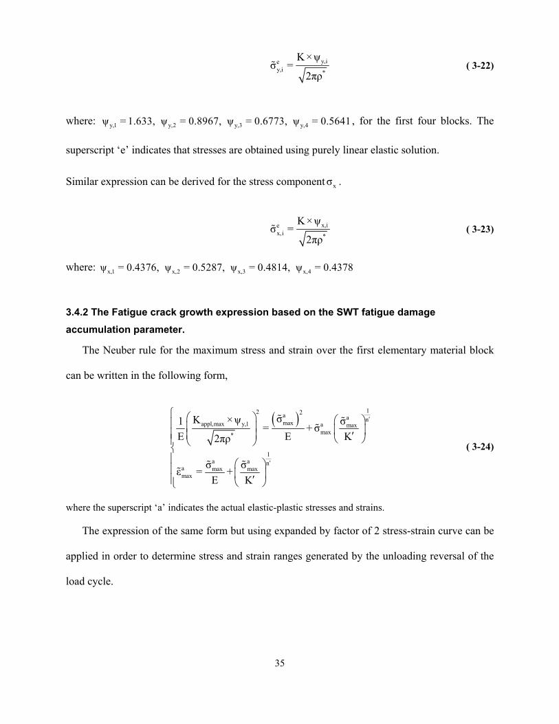
35
y,iey,i *
K×ψσ =
2πρ% ( 3-22)
where: , for the first four blocks. The
superscript ‘e’ indicates that stresses are obtained using purely linear elastic solution.
y,1 y,2 y,3 y,4ψ = 1.633, ψ = 0.8967, ψ = 0.6773, ψ = 0.5641
Similar expression can be derived for the stress component . xσ
x,iex,i *
K×ψσ =
2πρ% ( 3-23)
where: x,1 x,2 x,3 x,4ψ = 0.4376, ψ = 0.5287, ψ = 0.4814, ψ = 0.4378
3.4.2 The Fatigue crack growth expression based on the SWT fatigue damage accumulation parameter.
The Neuber rule for the maximum stress and strain over the first elementary material block
can be written in the following form,
( )12 2a a nmaxappl,max y,1 a max
max*
1a a n
a max maxmax
σK ×ψ σ1 = +σE E2πρ
σ σε = +E K
K
′
′
⎧ ⎛ ⎞ ⎛ ⎞⎪ ⎜ ⎟ ⎜ ⎟⎪ ⎜ ⎟ ′⎝ ⎠⎪ ⎝ ⎠⎨⎪ ⎛ ⎞⎪ ⎜ ⎟′⎪ ⎝ ⎠⎩
% %%
% %%
( 3-24)
where the superscript ‘a’ indicates the actual elastic-plastic stresses and strains.
The expression of the same form but using expanded by factor of 2 stress-strain curve can be
applied in order to determine stress and strain ranges generated by the unloading reversal of the
load cycle.

36
( ) ( )12 2a a n
appl y,1 a
*
1a a a n
ΔσΔK ×ψ1 Δσ= + 2 ΔσE E2πρ
Δε Δσ Δσ= +2 2E 2K
2K
′
′
⎧ ⎛ ⎞ ⎛ ⎞⎪ ⎜ ⎟ ⎜ ⎟⎪ ⎜ ⎟ ′⎝ ⎠⎪ ⎝ ⎠⎨⎪ ⎛ ⎞⎪ ⎜ ⎟′⎪ ⎝ ⎠⎩
% %%
% % %
( 3-25)
Equations 3-24 and 3-25 offer an unique relationship between the applied stress intensity
factor and the actual strains and stresses at the crack tip providing there are not any additional
factors which may alter those equations. Unfortunately, it has been shown already (Section 3.3.2)
that the compressive stresses induced by preceding loading cycles may exist in the material, and
therefore they have to be accounted for. The corrected for the residual stress effect total
maximum stress intensity factor and the stress intensity range give the final set of equations
enabling determination of the actual elastic-plastic crack tip strains and stresses.
( )
( ) ( )
12 2a a nmaxmax,tot y,1 a maxmax*
1a a n
a max maxmax
12 2a a ntot y,1 a
*
1a a a n
σK ×ψ σ1 = +σE E2πρ
σ σε = +E K
ΔσΔK ×ψ1 Δσ= + 2 ΔσE E2πρ
Δε Δσ Δσ= +2 2E 2K
K
2K
′
′
′
′
⎧ ⎛ ⎞ ⎛ ⎞⎪ ⎜ ⎟ ⎜ ⎟⎪ ⎜ ⎟ ′⎝ ⎠⎪ ⎝ ⎠⎨⎪ ⎛ ⎞⎪ ⎜ ⎟′⎪ ⎝ ⎠⎩⎧ ⎛ ⎞ ⎛ ⎞⎪ ⎜ ⎟ ⎜ ⎟⎪ ⎜ ⎟ ′⎝ ⎠⎪ ⎝ ⎠⎨⎪ ⎛ ⎞⎪ ⎜ ⎟′⎪ ⎝ ⎠⎩
% %%
% %%
% %%
% % %
( 3-26)
Eq. 3-26 makes it possible to determine the actual elastic-plastic stresses and strains in the first
elementary material block ahead of the crack tip.
The maximum stress and the strain range have to be combined in the next step into one
fatigue damage parameter (Eq. 3-3). After including the SWT damage parameter into the

37
Manson-Coffin strain-life fatigue curve the following expression is obtained relating the SWT
damage parameter to the number of cycles to failure for the first elementary material block.
( ) ( ) ( )2'a
2b b+cfa 'max f f f f
σΔεσ = 2N +σ ε 2N2 E%
% ' ( 3-27)
Eq.3-26 and Eq.3-27 provide direct link between the applied loading parameters and the number
of cycles to failure of the first elementary material block. When the number of cycles to failure
of the first elemental block is determined the instantaneous fatigue crack growth rate can be
determine from Eq. 3-4
Unfortunately, closed form solution to Eq. 3-26, Eq. 3-27, and Eq. 3-4 is not feasible;
however, approximate closed form solutions can be obtained at certain limiting conditions when
the elastic or plastic terms can be neglected. In both cases the closed form solutions have the
same form,
( ) ( )γp 1-p
max,tot totda = C K ΔK wh dN
⎡ ⎤⎣ ⎦
ere : ( 3-28)
'
'
1-b+c
2*
n +3' ' *n +1f f
1.633 n' 2C = 2ρ ; p = ; γ = - ;n' +1 b + c
2 σ ε πEρthaway from the K region
⎛ ⎞⎜ ⎟⎝ ⎠⎡ ⎤
⎢ ⎥ Δ⎢ ⎥⎢ ⎥⎣ ⎦
1-2 2b*
* 2f
1.633 1C = 2ρ ; p = 0.5; γ = - ;4πρ σ b thin the near K region
⎡ ⎤Δ⎢ ⎥′⎣ ⎦
The parameter ‘p’ is not constant and it varies between the two limits given above. Its
magnitude depends on the level of the plastic strain ahead of the crack tip. However, it has been
noticed that the maximum strains ahead of fatigue crack tips were predominantly plastic while
the strain ranges had significant elastic strain contribution. Therefore a variety of exponents were
analysed with the aim of finding one set of values for the entire fatigue crack growth curve. One

38
of such ‘mixed’ driving forces was proposed in the original two parameter driving force model
described in reference [39].
( ) ( )γp 0.5
max,tot totda n'= C K ΔK where : p =dN n' +1
⎡ ⎤⎣ ⎦
(3-29)
However, it was shown for several materials that fatigue life predictions based on Eq.3-28
with empirically fitted parameter ‘p’ better coincided with experimental fatigue crack growth
measurements than those based on Eq. 3-29. Therefore, Eq. 3-28 has been finally chosen for
fatigue crack growth analysis under variable amplitude loading histories.
Another interesting observation concerning equation 3-28 is how the fatigue crack growth
rate depends on cyclic stress-strain material properties. For materials with relatively flat cyclic
stress-strain curve (close to elastic - perfectly plastic) the cyclic strain hardening exponent, n’,
and the FCG parameter, p, are small. Therefore, fatigue crack growth rate depends mostly on the
total stress intensity range and the effect of the mean stress (or Kmax) is not significant.
The two parameter fatigue crack growth driving force of Eq. 3-28 is very similar to that one
proposed by Walker (Eq. 2-10). However, the main difference is that residual stresses due to
reverse plastic deformations are being accounted for in Eq. 3-28.
The two parameter driving force model has been developed and verified by Noroozi and
Glinka [2, 39] for constant amplitude loading with and without single overloads. In such cases
the compressive stress fields induced by each cycle are the same, and therefore they do not
require any additional modifications. However, in the case of variable amplitude loading, each
loading cycle creates its own stress field ahead of the crack tip which has to be accounted for
with respect to the current loading cycle and instantaneous crack tip position. The main purpose

39
of the presented work is to extend the two parameter driving force model for arbitrary variable
amplitude loading spectra.
It has been stated in Chapter 1 that the proposed model is applicable for the analysis of both
the crack initiation and the fatigue crack growth stage. According to the model, the number of
cycles required to create in a smooth specimen a crack of the size ρ* is equal to the number of
cycles needed to initiate the crack. The number of cycles necessary for such a crack initiation can
be obtained experimentally from testing smooth specimens in strain controlled conditions.
Therefore, the smallest crack which can be analysed is of the size of the elementary material
block, ρ*. Unfortunately, the classical fracture mechanics solution (Creager-Paris) based on the
stress intensity factor concept cannot be used directly in the analysis of such short cracks. Elastic
and subsequent elastic-plastic stresses and strains must be determined using different analytical
or numerical methods (FE analysis for example).
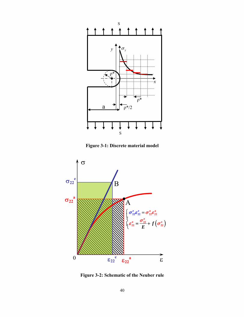
40
Figure 3-1: Discrete material model
Figure 3-2: Schematic of the Neuber rule
ε22e ε22
a
σ22e
σ22a
0
σ
ε
B
A
(22
22 22ee
fE
σ ε⎧ =⎪⎨⎪⎩
)22 22
22 22
a a
aa
a
σ ε
σε σ= +
S
S
ρ*
a ρ*/2
yσy
x
ρ*

41
Figure 3-3: Stress distributions ahead of the crack tip at various load levels
Residual stress field; Al 7075 T6, ΔK=Kmax=10 MPa√m
-800
-700
-600
-500
-400
-300
-200
-100
0
0 0.00001 0.00002 0.00003 0.00004 0.00005 0.00006 0.00007 0.00008Distance from the crack tip, x [m]
Res
idua
l str
ess
[MPa
]
Residual stressdistribution
Figure 3-4: Residual stress distribution obtained using the Neuber rule; Al 7075 T6 alloy ,
ΔK=Kmax=10 MPa√m
R>0.5 R<0.5
Load
Cycles
x
σ
Compressive stresses
Current crack
tip position
Region of integration, x0
42
Chapter 4
Determination of the Elementary Material Block Size, ρ*
The very important and initially unknown parameter in the model discussed above (Eq. 3-28) is
the finite crack tip radius, ρ*. Therefore a reliable method of its determination needs to be
developed and validated. For this purpose several approaches are presented and discussed below
including the list of their advantages and disadvantages.
Thus, the discussion presented below is mostly focused on various methods of determination
of the elementary material block size, ρ*, and the importance of that parameter with regards to
the proposed extension of the two parameter driving force model. The modified and extended
model has been named below as the UniGrow fatigue crack growth model. Experimental fatigue
crack growth data sets for two aluminium alloys (7075 T6 and 2324 T3) were used for the
illustration of the method of determination of the elementary material block size, ρ*. Determined
ρ* values were used later for fatigue crack growth predictions under both constant and variable
amplitude loading spectra.
4.1 The Method based on the fatigue limit and the threshold stress intensity range; (Method #1)
The first method of determination of the elementary material block size was proposed by
Glinka and Noroozi [2] and it requires the knowledge of the fatigue limit and the threshold stress
intensity range. It was postulated in this method that the fatigue crack would not grow under the
applied stress intensity ranges equal or less than the threshold stress intensity range, i.e.
when appl thK KΔ ≤ Δ , and therefore the stress range over the first elemental material block at the
crack tip should be simultaneously equal or less than the fatigue limit, i.e. aappl thσ σΔ ≤ Δ . Since

43
the fatigue limit is less than the yield limit the linear elastic analysis is only required and as a
result the following expression can be obtained from eq. (3-12).
*
1.6332
a thth
Kσπρ
Δ ×Δ = ( 4-1)
The elementary material block size, *ρ , can subsequently be expressed as:
22* 1.633
2thath
Kρπ σ
⎛ ⎞Δ= ⎜ Δ⎝ ⎠
⎟ ( 4-2)
It was found later that elementary material block sizes, determined from Eq. 4-2, were close to
the well known micro-structural parameter resulting from the Kitagawa diagram [51].
The method described above provides relationship between the elementary material block
size and fatigue properties of the material. Unfortunately, it requires very accurately determined
threshold stress intensity range and the fatigue limit which are not always readily available.
Additional care must be also taken so the fatigue limit, athσΔ , and the threshold stress intensity
range, are obtained under the same stress ratio R. An additional ambiguity also arises from
the fact that the stress intensity range is not the only parameter driving fatigue cracks. It has been
pointed out by Vasudevan et. al. [
thKΔ
52] that there are two different threshold parameters, namely
the maximum threshold stress intensity factor and the threshold stress intensity range and both
should be simultaneously exceeded for the crack to grow. Therefore it is not certain which
threshold should be used to determine the elementary material block size.
Lastly, the method described above neither proves nor disproves whether the elementary
material block size, *ρ , is only a material constant or it also depends on the applied load and
specimen/crack geometry. It must also be verified that the ρ* value obtained from Eq. 4-2 does

44
not depend on the stress ratio at which the fatigue crack growth threshold and the fatigue limit
were determined.
4.2 The Method based on the experimental fatigue crack growth data obtained at various stress ratios; (Method #2)
Because of several uncertainties discussed above the following alternative method based on
the experimental fatigue crack growth data has been proposed.
Since the mean stress effect has been already accounted for by using the SWT fatigue
damage parameter, all experimental fatigue crack growth rate data points plotted as a function
the total two-parameter driving force, (1 )max,p p
tot totK Kκ −Δ = Δ
tot
, should collapse onto one ’master’
curve. The total two-parameter driving force, κΔ , can be presented on the other hand as a
function of the elementary material block size, *ρ .
( ) ( )
( ) ( )1(1 )
max, max,
1
max, 0 0( | *) ( , ) ( | *) ( , )
( *)
p pp p ptot tot appl r appl r
p pa apappl r appl r
K K K K K K
K x m a x dx K x m a x
κ
σ ρ σ ρ
κ ρ
−−
−
Δ = Δ = + Δ + =
= + ⋅ Δ + ⋅
= Δ
∫ ∫ dx
Since the ρ* is the only unknown parameter in the equation above, it has to be such that all
experimental constant amplitude FCG data points obtained at various stress ratios R should
collapse onto one da/dN vs. Δκtot ‘master’ curve as shown in Figure 4-1.
The ‘master’ curve shown in Figure 4-1 can be considered as theoretical idealisation of the
actual engineering model. In practice it would be a set of points deviating around some mean
value due to the natural scatter of the experimental fatigue crack growth data (Figure 4-2).
Assuming some value of 1* *ρ ρ= and performing all of the steps shown in Figure 4-1
(assume ρ*, find σr, find Kr, and find Δκtot) it is possible to present FCG rate data in terms of the

45
total two-parameter driving force and fit by the mean (‘master’) curve using the least square
method (Figure 4-2b). However, the scatter of experimental FCG rate data shown in Figure 4-2b
is relatively big. Therefore, the usual error minimization problem has to be solved in order to
find such elementary material block size, *ρ , that experimental FCG rates presented in terms of
corresponding driving force have the smallest scatter (Figure 4-2c).
It should be mentioned that the method described above does not explicitly provide from the
fatigue fracture point of view information about the ρ* parameter as the elementary material
block size. The ρ* parameter represents only an effective crack tip radius influencing
subsequently the magnitude and distribution for the residual stress field.
It is also not clear whether the ρ* parameter is unique according to this method. The method
can be applied only if sufficient experimental fatigue crack growth data is available (i.e. constant
amplitude da/dN data obtained at three stress ratios at least).
The advantage of using the method discussed in the current section 4.3 is that parameters C
and m in the crack growth equation (Eq. 3-28) are determined form experimental fatigue crack
growth data and not from approximate expressions and smooth specimen fatigue data.
Advantages of using the approach discussed above are shown in Figure 4-3. It is clear that by
fitting the C and m parameters into limited amount of experimental fatigue crack growth data the
final equation simulates all other data much better than the theoretically derived approximate
formula (Eq. 3-28).
The collapsed experimental fatigue crack growth data is shown together with analytical and
fitted ‘master’ curves for the same *ρ . Since parameters ‘C’ and ‘m’ for analytical curve have
been estimated in two limited cases where either plasticity or elasticity effects were omitted, the
curve does not fit well the experimental FCG data in the region where both plasticity and

46
elasticity are important. Therefore, it can be concluded that the Eq. 3-28 provides only empirical
relation between the instantaneous FCG rate and total SIFs, however, it is preferable to fit
parameters ‘C’ and ‘m’ based on the experimental FCG data.
4.3 The Method based on the Manson-Coffin fatigue strain-life curve and limited fatigue crack growth data; (Method #3)
The third method of estimating the elementary material block size, ρ*, is based on two
assumptions:
♦ First, fatigue crack growth is understood as a series of re-initiations resulting in breaking
ahead of the crack tip subsequent elementary material blocks of size, ρ*. This assumption
allows to quantify the instantaneous fatigue crack growth rate as
*dadN N
ρ= ( 4-3),
where N is the number of cycles required to break the first elementary material block ahead
of the crack tip (see Figure 3-1).
♦ Second, the elementary material block size ρ* is a material constant and does not depend on
the specimen/crack geometry or applied loading conditions.
The procedure resulting in the determination of the ρ* parameter is summarized below.
Let us assume that we have experimental constant amplitude fatigue crack growth rate data and
corresponding applied stress intensity ranges (Figure 4-4) and the stress ratio R. This
information is sufficient for the determination of the applied stress intensity range, and the
maximum applied stress intensity factor for each particular data point.

47
As far as the stress state over the first elementary material block is concerned, it can be
noticed that there is only one non-zero stress component. Therefore, the crack tip stress/strain
analysis can be reduced to the uni-axial stress state.
Combination of the Ramber-Osgood material stress-strain curve (Eq. 3-1) and the Neuber
rule (Eq. 3-6) leads to the following expression:
122 n
max,tot max maxmax*
K ×1.633 ( )1 = +E E2πρ
σ σσK
′⎛ ⎞ ⎛ ⎞⎜ ⎟ ⎜ ⎟⎜ ⎟ ′⎝ ⎠⎝ ⎠
( 4-4)
Eq. 4-4 makes it possible the determination of the maximum elastic-plastic stress over the
first material block ahead of the crack tip as a function of the applied maximum stress intensity
factor. A similar expression can be obtained for the elastic-plastic stress range produced by the
unloading reversal.
2 12 n
tot*
ΔK ×1.6331 (Δ ) Δ= + 2(Δ )E E2πρ
σ σσ2K
′⎛ ⎞ ⎛ ⎞⎜ ⎟ ⎜ ⎟⎜ ⎟ ′⎝ ⎠⎝ ⎠ ( 4-5)
The elastic-plastic strain range can be subsequently determined from the expanded by factor of
two cyclic stress/strain curve:
1nΔ Δ Δ= +
2 2E 2Kε σ σ ′⎛ ⎞
⎜ ⎟′⎝ ⎠ ( 4-6)
Finally, the maximum stress and the actual strain range have to be combined using the Smith-
Watson-Topper (SWT) fatigue damage parameter in order to find the number of cycles required
to break the first elementary material block.
( ) ( )2
b cfmax f
σΔε σ = 2N + ε σ 2N2 E
′′ ′ ( 4-7)

48
The set of equations from Eq. 4-3 to Eq. 4-7 provides the solution to five unknown variables,
i.e. . Therefore, the elementary material block size ρ* can be determined
for each particular point of the experimental fatigue crack growth rate curve.
maxΔσ,σ ,Δε, N, and ρ*
It is very important to note that Eq. 4-4 and Eq. 4-5 contain the maximum total stress
intensity factor and the total stress intensity range, but not the applied ones. However, since the
elementary material block size and corresponding residual stresses are not known yet, the applied
stress intensity factors can be used only as the input for the first iteration.
Subsequent solutions of the set of equations from Eq. 4-3 to Eq. 4-7 for each experimental
FCG data point provide elementary material block sizes as a function of the applied stress
intensity ranges (Figure 4-5) corresponding to specific measured fatigue crack growth rates. It
can be noticed (Figure 4-5) that the elementary martial block size is not constant and it depends
on the load level. Therefore it contradicts the basic assumption of the model that the ρ*
parameter was supposed to be a constant parameter characteristic for a given material. The
apparent dependence of the ρ* parameter on the load is the result of using applied stress intensity
factors in the set of equations from Eq. 4-3 to Eq. 4-7 without accounting for residual stresses
induced in due course around the crack tip. Therefore, residual stresses induced ahead of the
crack tip during the first iteration should be accounted for in the next iteration resulting in a more
accurate estimation of the ρ* parameter. It means that after the first iteration instead of applied
the total stress intensity factors are used by accounting for the residual stress obtained during the
preceding iteration. This way new values of the ρ* parameter are obtained after each iteration.
The iteration procedure is complete when approximately the same value of the ρ* parameter is
obtained for all experimental data points.

49
Surprisingly, sometimes only two iterations are sufficient in order to obtain the same value of
the ρ* parameter for all experimental da/dN-ΔK data points, i.e. the ρ* value independent of the
load configuration.
The iteration process must be repeated in practice as many times as it is necessary to achieve
some kind of convergence (Figure 4-7) measured by the variation of individual of the average
parameter in such a way that avr,nρ* avr,n avr,n 1ρ* ρ* +≅ with required accuracy, where ‘n’ is the
number of iterations. The average value of the parameter is determined as the average of
all results obtained for the entire population of experimental data points
avr,nρ*
The method described above requires solving the system of five simultaneous nonlinear
equations Eq. 4-3 – Eq. 4-7 for each experimental fatigue crack growth data point. The number
of iterations necessary for obtaining the converged value of the *ρ parameter is usually ranging
from 5 to 10 iterations. The equation system can only be solved numerically. The method does
not require large amount of experimental data and sufficient estimation of the *ρ parameter can
be obtained using only few data points (>3)
It has been also shown that the elementary material block size obtained by the third method
does not depend on the stress ratio R. In other words, the same value of the ρ* parameter should
be obtained regardless of the stress ratio R at which the experimental constant amplitude fatigue
crack growth data was generated.
4.4 Summary of methods for the determination of the ρ* parameter
Table 4-1 provides the summary of all three methods for two aluminium alloys (7075 T6 and
2324 T3).

50
Table 4-1: The estimated values of *ρ
First method Second method Third method
Al 7075-T6 3.45381E-06 4.06184E-06 4.35938E-06
Al 2324-T3 2.53967E-06 3.94914E-06 3.34592E-06
Table 4-1shows that all three methods give relatively similar values of the elementary
material block size despite the fact that the first method is simpler but less accurate than the other
two methods. The advantage of the second method lies in the fact that in addition to the ρ*
parameter two constants ‘C’ and ‘m’ of Eq. 3-28, closely approximating the da/dN vs. Δκ data,
are also found. The third method can be used when only a small amount of experimental FCG
data is provided or part of the data is suspicious.
Because the ρ* parameters are not significantly different from each other regardless of the
method used it is difficult to recommend the best method. The choice of the method depends on
the data available. However, if sufficient constant fatigue crack growth data are available the use
of the second method is recommended because the resulting ρ*, C and m parameters closely
approximate the trend of basic experimental da/dN vs. Δκ data.
4.5 The effect of the elementary material block size on the residual stress intensity factor
It is apparent that the size of the elementary material blocks, ρ*, has an effect on the
calculated crack trip residual stresses, σr, and resulting residual stress intensity factor Kr.
Subsequently, the residual stress intensity factor, when included into the driving force, influences
predicted fatigue crack growth rate. Therefore it is important to estimate the effect of the error or
variation of the ρ* parameter on the predicted fatigue crack growth rate.

51
Therefore, several elementary material block sizes, *ρ , were analysed in order to evaluate
differences between corresponding residual stress distributions and resulting residual stress
intensity factors. The analysis was performed for the Al 7075-T6 alloy, Kmax,appl =10 MPa√m,
Kmin,appl =2 MPa√m. (Figure 4-8). The fatigue crack growth properties (Eq. 3-28) were p=0.1 and
γ=3.5.
The reference residual stress distribution was obtained for the parameter of *ρ =4e-6 m. The
lower σr vs. x curve, shown in Fig. 4-7, was determined for *ρ =8e-6 m and the upper one for
*ρ =2e-6 m. All three residual stress distributions have different magnitudes but character of the
distribution remains the same. The difference between the lowest and highest residual stress
magnitudes was approximately 9%. After including the difference into the total stress intensity
factors (Eq. 3-12 and Eq. 3-13) the difference in the predicted fatigue crack growth was
calculated from Eq. 3-28.
( )( )
( ) ( )
( ) ( )( ) ( )
( ) ( )
3.5 3.50.1 0.9 0.1 0.9,max ,1 ,1* 4 6 1
3.5 3.50.1 0.9 0.1 0.9
,max ,2 ,2* 2 6 2
10 2.22 8 2.221.127
10 2.42 8 2.42
appl r appl re
appl r appl re
da C K K K KdNda C K K K KdN
ρ
ρ
= −
= −
⎡ ⎤ ⎡ ⎤− Δ − − −⎢ ⎥⎣ ⎦ ⎣≈ ≈⎡ ⎤ ⎡ − −− Δ − ⎣ ⎦⎢ ⎥⎣ ⎦
⎦ =⎤
It appears that the dependence of the fatigue crack growth rate on the accuracy of the ρ*
parameter is not very strong because twofold (200%) change of the ρ* parameter resulted in less
than 13% difference in predicted fatigue crack growth rates.

52
Figure 4-1: Estimation of the elementary material block size based on the experimental fatigue crack growth data (Method #2)
Figure 4-2: Iteration process for the elementary material block size estimation based on the
Method #2 using linear ‘master’ curve
Log(ΔK) Log(Δk)
Step 1
ρ*1
Scatter
Log(Δk)
Step n
ρ*n
ScatterScatter
a) Initial FCG rate data without residual stress effect Impossible to describe using one ‘master’ curve
b) FCG rate data in terms of the total two-parameter driving force corresponding to the first approximation of ρ*
c) FCG rate data in terms of the total two-parameter driving force with smallest scatter
R1 R2
,2applKΔ
dadN
,1applKΔ applKΔ
, max, ,*, ,appl i appl iK Kρ Δ
1,2
dadN
( ), max,*, ,r i appl applK Kσ ρ Δ
( ), max,*, ,r i appl applK K Kρ Δ
1 2
dadN
κ κΔ = Δ
κΔ
R1 R2
1,2κΔ
1, 221

53
da/dN vs. ΔK; Al 7075-T6 (data of Newman and Jiang)
1.E-12
1.E-11
1.E-10
1.E-09
1.E-08
1.E-07
1.E-06
1.E-05
1.E-04
1.E-03
1 10 100
Δκ tot
da/d
N, [
m/c
yc].
Analitacal curves, limited cases
Fitted, Method 2
R=0.82..0.7
R=0.5R=0.33
R=0R=-1
R=-2
Figure 4-3: Analytical and fitted ‘master’ curves for Al 7075-T6 alloy (Exp. data [71, 73])
Figure 4-4: Schematic of experimental fatigue crack growth rate data
dadN
max,, ,appl applda K KdN
⎛ ⎞Δ⎜ ⎟⎝ ⎠
KΔ appl

54
ρ*
avr,1ρ*
applΔK
Figure 4-5: Elementary material block size as a function of the applied stress intensity range - after first iteration
ρ*
avr,1ρ*
1
2
avr,2ρ*
applΔK Figure 4-6: Elementary material block size as a function of applied stress intensity range
after two iterations

55
ρ*
avr,1ρ*
1
2
avr,2ρ*
avr,n 1ρ* +n+1
applΔK Figure 4-7 : Elementary material block size as a function of applied stress intensity range
after n+1 iterations when the convergence was reached
Residual stress distributions for different ρ *
-600
-500
-400
-300
-200
-100
0
0.E+00 1.E-05 2.E-05 3.E-05 4.E-05 5.E-05 6.E-05 7.E-05 8.E-05 9.E-05
Distance from the crack tip, [m]
Res
idua
l str
ess,
[MPa
] Sr(x) for r*=8e-6m
Sr(x) for r*=4e-6m
Sr(x) for r*=2e-6m
Kr=-2.020Kr=-2.226
Kr=-2.425
Figure 4-8: Residual stress distributions obtained for different values of the elementary material block size; Al 7075 T6

56
Chapter 5 Two-parameter Total Driving Force Model for Variable Amplitude
Loading Spectra – the UniGrow Fatigue Crack Growth Model
It has been shown in Chapters 2 and 3 that fatigue crack growth depends on several factors
such as the load, geometry of the cracked body and the size and geometry of the crack. All of
them are combined into one parameter i.e. the stress intensity factor. According to the proposed
model the applied maximum stress intensity factor, Kappl,max, the applied stress intensity range,
ΔKappl, have to be combined with the residual stress intensity factor, Kr, accounting for the effect
of crack tip residual stresses. The weight function technique [49] described in Chapter 3 was
shown to be one of the easiest and most versatile ways of determining the residual SIF induced
by the crack tip compressive residual stress.
Based on the experimental observations [1, 23] it was concluded that the fatigue crack
growth depends, in the case of variable amplitude loading, not only on the current residual stress
field generated by the current cycle but also on those residual stress fields generated by the
preceding loading history and left behind the crack tip. Therefore, the correct estimation of both
the resultant residual stress produced by all previous loading cycles and corresponding residual
stress intensity factor becomes one of the most important (and complicated) part of the variable
amplitude crack model discussed below and subsequently named as the UniGrow model.
The near crack tip stress distributions generated by subsequent loading cycles can be
determined using the Neuber [40] or Glinka rule [41] as explained earlier. However, in the case
of variable amplitude loading, the minimum and maximum stresses induced by the current
loading cycle are not necessarily the ones influencing the instantaneous FCG.

57
5.1 The Maximum stress memory effect
As far as the constant amplitude loading is concerned there is no problem in defining the
maximum stress or the maximum stress distribution near the crack tip because it is always the
stress or exactly speaking the stress distribution induced by the current maximum load level.
This statement holds for loading histories with constant amplitude stress intensity factor and
constant amplitude cyclic loads in general. However, in the case of variable amplitude loading
histories the current maximum crack tip stress does not necessarily correspond to the current
maximum load level because higher crack tip stresses might have been induced by previous
loading cycles. As a consequence the current maximum stress to be considered might be the
stress generated by previous load cycles like in the case of the load history shown in Figure 5-1:
The stress distribution corresponding to the maximum load level 1 (Figure 5-2) can be
determined using the Neuber [40] or Glinka [41] rule and the cyclic stress-strain curve. Because
the load cycle with the maximum at point 1 is the first cycle in the history, the crack tip stress
corresponding to the load level 1 is the maximum stress distribution.
By carrying out the same procedure for the second load cycle the maximum stress
distribution corresponding to the load level 3 can be determined as well. However, the crack has
already propagated during the first loading cycle and therefore the crack tip stress field induced
by the second load cycle is created at different location in the space and it is associated with the
new crack tip position. In this particular case the crack tip stresses corresponding to the load
level 3 (Figure 5-3) are higher than stresses in the previous distribution. As a consequence, the
current maximum crack tip stress distribution is the maximum stress to be used for the
subsequent calculation of the compressive minimum stresses and the instantaneous fatigue crack
growth rate.

58
Let assume that crack tip stresses corresponding to load the level 5 are less (Figure 5-4) than
those corresponding to the load level 3. In such case, according to the model definition, the
previous maximum stress (at load 3) is the maximum stress to be considered for the current
loading cycle.
When the crack tip moves far enough from the location where the load level 3 was applied or
where the past high load was applied, it may happen that the crack tip stresses induced by the
current cycle exceeds the previous maximum stresses over only a part of the previous
distribution (Figure 5-5). In such a case the combined maximum stress field should be used in
subsequent analysis.
5.2 The resultant minimum stress field and the residual stress intensity factor
Now, let consider how residual stresses σr(x) created by the past variable amplitude loading
history should be transformed into the instantaneous residual stress intensity factor Kr. Because
the same mathematical and numerical procedure. i.e. the multiaxial Neuber rule is used for each
cycle it is expected that each cycle of the constant amplitude loading spectrum produces the
same type of stress field ahead of the crack tip.
Let us analyse the crack tip stress-strain response due to several consecutive reversals of an
arbitrary variable amplitude loading history as that one shown in Figure 5-6. Application of the
tensile load reversal from point 1 to point 2 may extend the fatigue crack over an interval Δa and
therefore, the maximum stresses corresponding to the maximum load level 2 have to be
combined with the new crack tip position. It is subsequently assumed that the fatigue crack does
not grow during the unloading reversal from load level 2 to load level 3. Therefore the static
notch analysis (see Chapter 3) can be used to determine the minimum stress distribution
corresponding to the minimum load level 3. The next load reversal (3 - 4) may again propagate

59
the crack by the next increment Δa and a new compressive minimum stress field is created at the
load level 5. However, it is important to remember that the stress intensity factor resulting from
the application of the load reversal (3 - 4) should be reduced due to the presence of the
compressive (residual) stresses left behind the crack tip resulting in the reduction of the fatigue
crack growth rate.
Based on experimental observations of fatigue crack behaviour under variable amplitude
loading [1, 23, 53] it was noticed that the residual stress intensity factor for the current cycle was
not only dependent on the residual stress field ahead of the crack tip induced by the last cycle,
but it could also depend on the residual stress fields produced by preceding cycles of the applied
loading history. Such a phenomenon called later as the structural memory effect has to be taken
into account while calculating fatigue crack growth increment caused by the current load cycle.
Therefore it is necessary to define when the effect of previous cycles can be neglected due to the
fact that the crack tip has propagated out of its zone of influence.
Based on the observation of available experimental data a new methodology for obtaining the
residual stress intensity factor for the current load cycle has been proposed. All crack tip stress
distributions induced by previous cycles have to be combined, according to the proposed
methodology, into one resultant minimum stress field influencing the current fatigue crack
growth rate.
Four rules have been derived for the determination of the residual stress field in the crack tip
region.
• First, only the compressive part of the minimum stress distribution affects the fatigue
crack growth rate. The compressive part of the minimum stress distribution induced by
the first loading cycle constitutes the initial resultant minimum stress field used for the
60
determination of the residual stress intensity factor. The rule is schematically explained in
Figure 5-7 using simple variable loading history. Part 2 of the Figure 5-7 (and following
figures from 5-8 to 5-10) shows all actual residual stress fields induced through the
loading history. Part 3, on the other side, contains only these residual stresses which are
influencing the instantaneous FCG.
• Secondly, if the compressive part of the minimum stress distribution induced by
current loading cycle is completely inside of the previous resultant minimum
stress field, the material does not “feel” it and the current minimum stress
distribution should be neglected (Figure 5-8).
• Thirdly, if the compressive part of the minimum stress distribution of the current loading
cycle is fully or partly outside of the previous resultant minimum stress field they should
be combined as shown in Figure 5-9.
• The fourth rule states that, each minimum stress distribution is active and should be
included into the resultant one as long as the crack tip is inside its compressive stress
zone. In other words, when the crack tip has propagated across the entire compressive
stress zone of given minimum stress field it should be neglected (see the Figure 5-10).
A simple variable loading history and compressive minimum stress distributions induced by
individual cycles are shown in Fig. 5-10 (Part 1 and Part 2). Let assume that the crack tip has
propagated through the zone of influence of first three cycles up to the point ‘a’. The minimum
stress distributions corresponding to load levels 2, 4, and 6 have to be, according to the fourth
rule, excluded from the resultant minimum stress field and subsequent fatigue crack growth
analysis.

61
5.3 The UniGrow analysis of simple loading spectra
5.3.1 Constant amplitude loading
The four rules established in the previous section allow finding the resultant minimum stress
field corresponding to the current loading cycle. However, before trying to predict the fatigue
crack growth and fatigue crack propagation life under variable amplitude loading one has to be
sure that the model correctly predicts the fatigue crack growth and fatigue crack propagation life
in the case of simple loading histories.
Let us consider a tension to tension constant amplitude loading history, the resulting
minimum crack tip stress distributions, and the evolution of corresponding residual stress
intensity factor Kr (Figure 5-11). Each loading cycle extends the crack by certain increment and
generates a compressive minimum stress distribution associated with the current crack tip
position similar to the previous one. The similarity can be attributed to the fact that the crack size
increments and the increase of the applied stress intensity factor after each loading cycle are
relatively small under constant amplitude loading history.
As long as the crack does not propagate out of the first cycle zone of influence (denoted as
point ‘S’ in Figure 5-11) each cycle of the constant amplitude loading history contributes the
same amount of stresses into the resultant minimum s stress field and corresponding residual
stress intensity factor. However, if the crack tip is outside of the first cycle zone of influence the
same amount will be added to (by the third rule) and subtracted from (by the fourth rule) the
minimum resultant stress field. It means that under constant amplitude of the stress intensity
factor the residual stress intensity factor Kr is, according to the UniGrow model, also constant.

62
5.3.2 Constant amplitude loading history interrupted by a single overload or underload
Similar as previously constant amplitude loading history but interrupted by relatively high
tensile overload, associated minimum stress distributions, and the evolution of corresponding
residual stress intensity factor are shown in Figure 5-12.
It should be noted, that the compressive minimum stress distribution generated by the
overload is higher in magnitude than the compressive minimum stress distributions generated by
the base constant amplitude loading cycles. Therefore, the application of a high tensile overload
resulted in the decrease of the fatigue crack growth called often as the retardation effect. The
existence of the fatigue crack growth retardation phenomenon has been confirmed by a wide
variety of experimental data [53].
The residual stress effect resulting from a single overload extends, due to the larger zone of
influence, over much larger region (and time interval) than those generated by the base loading
cycles. However, as soon as the crack propagates through the region of the highest in magnitude
residual stresses induced by an overload the residual stress intensity factor starts decaying and
should eventually reach the same stabilised level as that one generated by the base constant
amplitude loading.
Let consider now the same tension to tension constant amplitude loading history interrupted
by single under-load (Figure 5-13), and analyze the compressive minimum stress distribution at
the minimum under-load load level (2).
It can be noticed again that the minimum stress distribution corresponding to the absolute
minimum load level (2) is greater in the magnitude than that one generated under similar
constant amplitude loading. However, experiments show that under-loads do not create

63
retardation effect as the overloads do and they can even cause a slight acceleration of the fatigue
crack growth [57].
The correct interpretation of the crack tip stress-strain affairs is that the minimum residual
stress induced by an under-load cycle should not be later associated with the minimum load level
of the under-load but with the minimum load level of following base loading cycles. In order to
clarify this idea let us consider stress/strain material behaviour of non-growing crack under
constant amplitude loading history interrupted by a single overload or a single under-load
(Figure 5-14). In the first case (overload), the minimum stress distribution corresponding to an
overload and the minimum stress corresponding to the following constant amplitude base loading
cycles are the same and less than the minimum stress due to preceding CA loading cycles (the
retardation effect of due to single overload). However, when an under-load is applied, the
minimum stress corresponding to the following constant amplitude base loading cycles is greater
than one at the minimum level of the under-load cycle (no retardation effect).
Therefore, it was concluded that the compressive minimum (residual) stress field associated
with the load level (2) in Figure 5-13 affects the fatigue crack growth caused only by the
immediate reversal just after the application of the under-load (2-3). However, the residual stress
at the minimum load level (4) of the next constant amplitude base loading cycle is less in
magnitude than that one at minimum level of the under-load. Therefore the following rule has
been adopted for the calculation of the compressive minimum stresses corresponding to the
minimum load level (4) the application of an under-load.
The minimum stress distributions at the load level (4) in Fig. 5-14 have to be determined
accounting for the minimum stresses generated by the previous under-load (2) but following the
cyclic stress-strain curve from load level (2) to (4). The compressive minimum stress distribution

64
corresponding to the current loading cycle (load level 4) is to be used for the determination of the
residual stress intensity factor Kr necessary for the calculation of subsequent crack growth
increments.
5.3.3 Loading spectra with single over- and uder-loads
The same rules apply in the case of stress histories containing both over- and under-loads
(Figure 5-15).
The compressive minimum stress distribution induced by the overload (1) effects the fatigue
crack growth up to the application of the reversal with the minimum load level at point (2).
During the application of the under-load another major compressive stress field was generated
after attaining the low load level (2). The compressive stress field created by the under-load may
sometimes overlap the compressive stress field created by the preceding overload (third rule).
However, according to the rule proposed in the previous section the stress field corresponding to
the load level (2) affects the fatigue crack growth caused only by the immediate reversal
following the uderload, i.e. the reversal following the load level (2). The fatigue crack growth
caused by the subsequent constant amplitude base loading cycles is affected by the minimum
stress distribution corresponding to the load level (3) which is relatively small in magnitude
when comparing with the minimum stress distributions induced by the overload or under-load.
Therefore, the retardation effect created by the overload (overloads) can be, depending on
relative magnitude and the stress-strain material behaviour in the crack tip region, fully or
partially eliminated by the following under-load reversal. Therefore, in the case of almost elastic
perfectly plastic materials (like Ti-17 alloy) even small under-loads can eliminate the beneficial
retardation effect of high tensile overloads.

65
Figure 5-1: Variable amplitude loading history
Figure 5-2: The Maximum stress distribution generated by the load level 1 (see Fig. 5-1)
Figure 5-3: The Maximum stress distribution generated by the load level 3
1
3
σmax
1
x
σ max
3 9
1 5 7
2 10 4 6 8
time
Loa
d
x

66
σmax
3
5
x
Figure 5-4: The Maximum stress distribution corresponding to the load level 5
σmax
x
3
9
Figure 5-5: Combined maximum stress distributions at load level 9

67
SIF Stress
x
Time Min. stresses at point 5
Crack tip at
points 2&3
Min. stresses at point 3
Max. Stresses at point 4
Max. Stresses at point 2
Crack tip at
point 1
5
4
3
2
1
Figure 5-6: Schematic of stress field corresponding to various load levels of variable
amplitude loading history
Figure 5-7: The First structural memory rule: 1) the loading history, 2) the actual stress
field ahead of the crack tip, 3) the resultant minimum stress field.

68
Figure 5-8: The Second structural memory rule: 1) the actual stress field ahead of the
crack tip, 2) the resultant minimum stress field.
Figure 5-9: The Third structural memory rule: 1) the actual stress field ahead of the
crack tip, 2) the resultant minimum stress field
3)
1)
8
1010
6 8 2 4 2)
11
108
7
6
5
4
3
2
1load
time
σmin σmin, aa
x x
Figure 5-10: The Forth structural memory rule: 1) the loading history, 2) stress fields
generated by subsequent loading cycles (from 1 to 10),
3) the resultant stress field.

69
σr B A
time
K
Kr(A) Kr(B)
x
x
S B A
Kr
A constant amplitude
applied loading
produces constant
residual SIF
Figure 5-11: Minimum compressive stress distributions generated by subsequent cycles of
constant amplitude stress intensity loading history
K B A OL
time
σr
x
x
B OL A
Kr(B) Kr(A)
Kr
A single overload creates high
compressive stresses and
increases the magnitude of the
residual SIF.
Figure 5-12: Minimum compressive stress fields for generated by a constant amplitude stress intensity factor history interrupted by a single tensile overload

70
σr
x
x
B UL A
Kr(B) Kr(A)
point 4
point 2
SIF
2
UL 4
31
time
Kr
A single under-load
reduces the magnitude of
the residual SIF.
Figure 5-13: Minimum compressive stresses generated by a constant amplitude stress
intensity factor loading history interrupted by a single under-load
Under-load
ε
σ
CA minimum UL minimum
CA & OL minimum
σ
ε
Overload
Figure 5-14: Stress/strain material behavior in the tip of a stationary crack
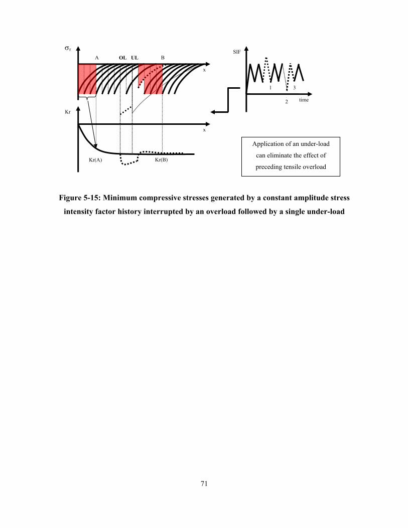
71
σr
x
SIF
time
x
Kr(A)
A
Application of an under-load
can eliminate the effect of
preceding tensile overload
OL
3 1
2
1
Kr(B)
B UL
Kr
Figure 5-15: Minimum compressive stresses generated by a constant amplitude stress
intensity factor history interrupted by an overload followed by a single under-load

72
Chapter 6 Fatigue Crack Growth Analysis under Spectrum Loading –
Predictions/ Experiments
Basic assumptions of the two-parameter driving force fatigue crack growth model
appropriate for analysis of fatigue crack growth under constant amplitude loading were described
in Chapter 3. Chapter 4 contains the set of ‘memory’ rules which are the core of the new
UniGrow fatigue crack growth model applicable for the analysis of fatigue crack growth under
arbitrary variable amplitude loading spectra. The UniGrow model accounts for the effect of
residual stresses generated around the crack tip due to reversed cyclic plastic deformations. All
numerical subroutines for calculating elastic plastic crack tip strains and stresses and algorithms
simulating the material and structural memory effects have been coded into one computer
software described in Appendix A. In order to verify the predictive capability of the UniGrow
model several analyses of fatigue crack growth have been carried out and compared with
experimental data.
The fatigue life analyses were carried out for the following geometry, load and spectra
configurations:
• Compact tension specimens made of Ti-17 alloy under constant amplitude loading
interrupted by under-loads (3 spectra),
• Central through crack specimen made of 350 WT steel under constant amplitude loading
interrupted by overloads (1 spectrum),
• Central through crack specimen made of Al 2024 T6 alloy under step-wise loading spectra
(2 spectra),

73
• Flanged plate made of Al 7010 T7 alloy with a central lightening hole weaken by a corner
defect on the inner edge under the ASTERIX loading spectrum (1 spectrum),
• Semi-elliptical crack at the wing attachment carry-through bulkhead made of Al 7050 T3
alloy under random predominantly tensile loading spectrum (F/A – 18 aircraft load
spectrum),
• Central through crack specimens made of Al 7075 T6 alloy under two random loading
spectra obtained for the P3 aircraft,
• Edge crack specimens made of Al 2324 T3 alloy under modified P3 aircraft loading spectra
(8 spectra).
The chart presented in Figure 6-1 shows the step – by – step procedure for fatigue crack
growth analysis and fatigue life estimation based on the UniGrow fatigue crack growth model.
All material, geometry and load spectrum cases listed above were analysed according to the
same procedure shown schematically in Figure 6-1. Due to large amount of material constants
and geometry and load configurations all numerical data have been extracted from the text and
summarized at the end of each section.
The stepwise procedure for the fatigue crack growth analysis based on the UniGrow fatigue
crack growth model was as follows (Figure 6-1):
1. Monotonic material properties such as the modulus of elasticity, E, and the Poisson ratio,
ν, and cyclic stress-strain material properties such as the cyclic hardening coefficient, K’,
and the cyclic strain hardening exponent, n’, have to be obtained from experimental
stress-strain data based on the standard procedure [54] for from available literature
sources.

74
2. The Manson-Coffin strain-life fatigue material properties have to be obtained from
experimental strain-life data according to the standard procedure [54] or taken from
available literature sources.
3. Constant amplitude fatigue crack growth data obtained at several different stress ratios
needs to be selected as a base for subsequent fatigue crack growth and fatigue life
analysis.
4. The magnitude of the elementary material block size parameter, ρ*, needs to be obtained
according to one of the methods described in Chapter 4.
5. Knowledge of the elementary material block size, ρ*, allows to find the residual stress
intensity factor, Kr, as a function of the applied stress intensity range, ΔKappl, (and the
maximum applied stress intensity factor, Kappl,max) for each stress ratio of the constant
amplitude fatigue crack growth data. It is somewhat surprising that the Kr vs ΔKappl
relationship is linear for all materials studied up to date.
6. Based on the estimated residual stress intensity factor all experimental constant amplitude
fatigue crack growth data points have to be presented in terms of the total driving force,
Δκtot, resulting in one ‘master’ da/dN –ΔK curve.
7. The da/dN –Δκ ‘master’ curve has to be subsequently divided into several regions which
can be approximated by linear elements in log-log scale using the linear regression
method. The ‘master’ curve makes it possible to determine the corresponding fatigue
crack growth rate da/dN for any value of the total driving force Δκ.
8. The applied loading spectrum has to be prepared. Fatigue life analysis can be performed
under any type of applied loading spectrum.
75
9. Appropriate generic crack configuration and component geometry have to be chosen for
the stress intensity factor calculation and fatigue life analysis.
10. After collecting all the data described in steps 1-9 the UniGrow software (Appendix A)
can be used for the fatigue crack growth prediction and fatigue life analysis.
Some additional comments can be made concerning the first two steps of the algorithm described
above. It has been shown [1] that some of parameters of the strain-life curve can be related to
parameters of the cyclic stress-strain curve.
( )'
' ''
fb c
f
bn and Kc
σ
ε= = ( 6-1)
Therefore, out of the six constants of the Manson-Coffin and the Ramberg-Osgood curve only
four are independent. However, it is common in practice to obtain all six of them separately
based on three different fits into the experimental data. In rare cases inconsistencies may occur
between parameters obtained from experimental data and Eq. (6-1). This could happen in
situations where the experimental data do not fit well assumed mathematical expressions. For
example, Fatemi et al. [55] showed that the standard linear Manson-Coffin approach cannot be
used for certain aluminium alloys.
6.1 Fatigue crack growth in the Ti-17 titanium alloy under constant amplitude loading spectra with under-loads
It has been shown by a number of researchers [56] that the application of a single underload
can cause noticeable acceleration of subsequent fatigue crack growth instead of the well know
retardation phenomenon. Unfortunately, most of the existing fatigue crack growth models
discussed briefly in Chapter 2, including the crack closure model [33], are not capable of

76
correctly simulating underload effects discussed above. Therefore, it is important to verify the
UniGrow fatigue crack growth model for cyclic loading spectra with underloads.
The set of experimental fatigue crack growth data, used in the analysis, was obtained by S.
M. Russ [57] with the aim to investigate the load-interaction effect in the case of constant
amplitude loading with repeatable single underloads. The fatigue crack growth was studied in
compact tension specimens (Figure 6-2) made of Ti-17 titanium alloy subjected to special type of
loading spectra shown in Figure 6-3. The stress intensity factor expression used in the study [57]
was:
2 3
3/ 2
20.886 4.64 13.32 14.72 5.6
1
aP a a aWK
W W W WB W aW
⎛ ⎞+⎜ ⎟ ⎡ ⎤⎛ ⎞ ⎛ ⎞ ⎛ ⎞ ⎛ ⎞⎝ ⎠= + − + −⎢ ⎥⎜ ⎟ ⎜ ⎟ ⎜ ⎟ ⎜ ⎟⎝ ⎠ ⎝ ⎠ ⎝ ⎠ ⎝ ⎠⎛ ⎞ ⎢ ⎥⎣ ⎦−⎜ ⎟
⎝ ⎠
4a
where B is the thickness of the specimen and W is the width.
As it could be seen, the baseline constant amplitude loading spectrum was periodically
interrupted by applying tensile underloads. All relevant data concerning analysed loading spectra
were borrowed from reference [57] and they are also shown in Table 7-1. These include the
maximum applied load, the ratio between maximum and minimum applied load of the baseline
loading cycles and the underloading levels, and the number of spacing cycles between
underloads.
The Ti-17 designation is the commercial name for the Ti-5Al-2Sn-2Zr-4Mo-4Cr alpha-beta
titanium alloy which was primary developed as a material for discs in turbine fans and
compressors working in temperatures below 427o C.
Cyclic stress-strain experimental data was also borrowed from reference [57]. The plastic
strain vs. stress amplitude data points were extracted from the experimental total strain vs. stress

77
data according to the standard procedure given in reference [54]. This data set was subsequently
fitted by the linear regression into the Ramberg-Osgood expression (Figure 6-4, Table 6-2).
Constants for the Manson-Coffin fatigue curve (Table 6-2) were taken directly from the
reference [57]. Four constant amplitude fatigue crack growth data sets obtained at four different
stress ratios [57] were selected as the reference for subsequent fatigue crack growth and fatigue
life analysis (Figure 6-5 (left)). The elementary material block size, ρ*, was obtained from the
Manson-Coffin fatigue curve, the Ramberg – Osgood strain-stress curve, and constant amplitude
fatigue crack growth data according to the third method described in Chapter 4. Two sets of ρ*
values, determined on the basis of two fatigue crack growth data sets obtained at two different
stress ratios, are shown in Figure 6-6 and the resultant value is listed in (Table 6-2). The
variation of the ρ* parameter is plotted once as a function the applied stress intensity factor and
second as a function of the total stress intensity range. It is apparent that one single value of the
ρ* parameter can be found for the entire range of fatigue crack growth rates when expressed in
terms of the total stress intensity range, i.e. when the residual stress effect is accounted for.
Based on the already obtained ρ* value the residual stress was determined for each constant
amplitude experimental da/dN data point and all experimental data points were finally presented
in terms of the total driving force resulting in one da/dN-Δκtot, ‘master curve’ as shown in Figure
6-5 (right). The ‘master curve’ was subsequently divided into three segments approximated by
three linear pieces in log-log scale by using the linear regression method. Numerical values of
parameters of the three curves are given in (Table 6-2).
Then the UniGrow fatigue crack growth program was used for calculating the fatigue crack
growth under various load histories as that one shown in Figure 6-3. The predicted and

78
experimental crack length vs. number of cycles (a-N) data sets are shown in Figure 6-7, Figure
6-8, and Figure 6-9 for all loading spectra listed in Table 6-1
The fatigue ‘a vs. N’ data sets shown in Figures 6-7 to 6-9 represent the experimental data,
the UniGrow predicted data for the history with underloads and the UniGrow predictions for the
base constant amplitude load history without any underloads. As one can notice, the proposed
fatigue crack growth model predicts the fatigue crack growth close to the experimental one. The
under-load effect is clearly shown by the difference in the fatigue ‘a vs. N’ curves obtained for
the loading spectrum with periodic underloads and for the baseline constant amplitude loading
history.
In the first case, the predicted fatigue ‘a-N’ curves based on the UniGrow model are almost
the same as the experimental fatigue life curves. The difference in the fatigue life between the
constant amplitude (R=0.4) loading spectrum and the spectrum with under-loads was around
45% at the final crack size a=25mm or, in other words, application of tensile under-loads
decreased fatigue life of the specimen almost by factor of 2. However, the residual stress
profiles, calculated according to the five rules formulated and discussed in Chapter 5, were
almost the same for the baseline and underload interrupted loading spectra. The acceleration of
the fatigue crack growth in the case of underload interrupted loading spectra is mostly due to
crack increments caused by high stress intensity ranges induced by relatively often applied
underloads (10 cycles apart).
Approximately the same qualitative results were obtained in the case of the second loading
spectrum (see Table 6-1) with underloads applied every 100 cycles. The predicted UniGrow
fatigue ‘a-N’ curves matched well (Figure 6-8) the experimental data and the difference between

79
the fatigue life predicted for the spectrum with underloads and the base constant amplitude
history was about 15% at the crack size of a=15mm.
The apparent decrease of the fatigue life caused by underloads was predominantly due to large
crack increments produced by large underload ranges and not necessary by significant change of
residual stresses.
Figure 6-9 shows also good agreement between the UniGrow predicted and the experimental
fatigue crack growth data for the third loading spectrum (Table 6-1 Figure 6-9). The fatigue
crack growth analysis under the base constant amplitude loading history was not carried out in
this case.

80
(1) (2 optional) (3)
Ramberg-Osgood
curve
Manson-Coffin
curve
CA FCG curve (Applied SIF range)
Elementary material block size
Linear residual SIF functions for each
CA FCG rate curves
CA FCG curve (total
driving force)
FCG constants Loading Spectrum Specimen description
UniGrow
Software
Fatigue crack growth prediction (11)
(10)
(8) (9) (7)
(6)
(5)
(4)
Figure 6-1: Step-by-step procedure for fatigue life analysis using the UniGrow model

81
Table 6-1: CA/Under-load loading spectra for Ti-17 alloy specimens (Figure 6-3)
Spectrum # Pmax, kN Rbl Rul Nbl/Nul
1 1.15 0.4 0.1 10
2 1.47 0.4 0.1 100
3 2.00 0.7 0.1 100
Table 6-2: Material properties of the Ti-17 titanium alloy
Constant Value Units Source
E 116935 MPa
K’ 1183 MPa
n’ 0.0276
σ’f 1172 MPa
b -0.017
ε'f 0.71219
c -0.61594
S.M.Russ PhD thesis [57]
p 0.026859 n/(1+n)
ρ* 7.00E-06 m The third Method (Chapter 4)
C1 6.00E-34
C2 1.00E-13
C3 3.00E-11
m1 59
m2 8.6327
m3 3.8976
Fitted into the experimental
CA FCG data [57] by the linear regression analysis,
see Figure 6-3 (right)

82
Figure 6-2: The compact tension specimen used in Russ’ experiments and subsequent analysis (all
dimensions are in mm, thickness=10mm) (Ref. [57])
Figure 6-3: Schematic of the constant amplitude spectrum with periodic underloads (Ref. [57])
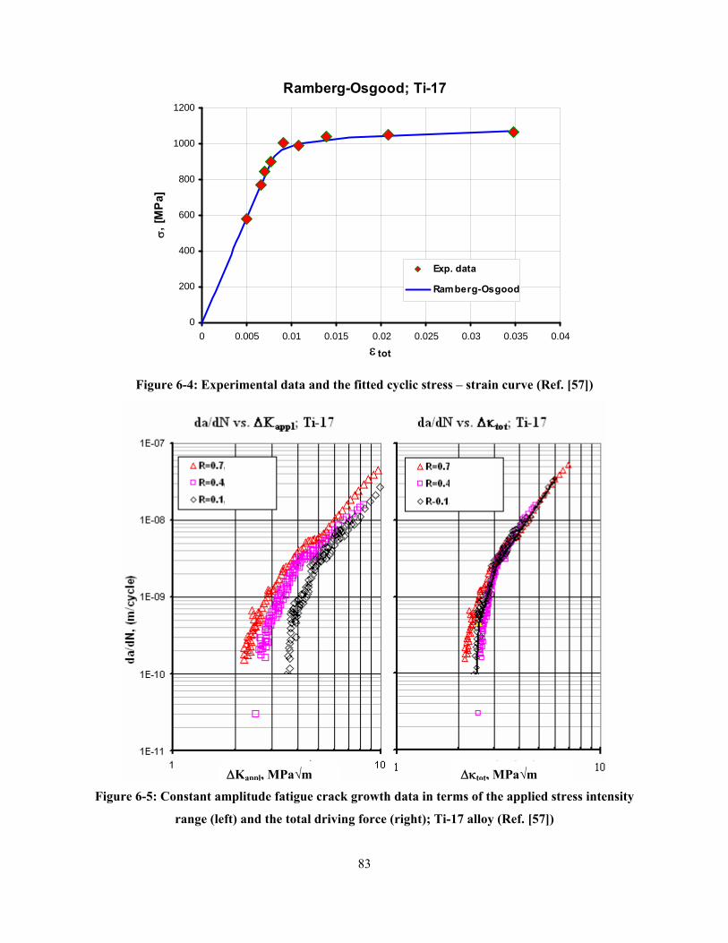
83
Ramberg-Osgood; Ti-17
0
200
400
600
800
1000
1200
0 0.005 0.01 0.015 0.02 0.025 0.03 0.035 0.04ε tot
σ, [
MPa
]
Exp. data
Ramberg-Osgood
Figure 6-4: Experimental data and the fitted cyclic stress – strain curve (Ref. [57])
ΔKappl, MPa√m Δκtot, MPa√m
Figure 6-5: Constant amplitude fatigue crack growth data in terms of the applied stress intensity
range (left) and the total driving force (right); Ti-17 alloy (Ref. [57])

84
Elementary material block size
0
0.00001
0.00002
0.00003
0.00004
0.00005
0.00006
0.00007
3 4 5 6 7 8 9 10 11Δκappl, [MPa]
ρ*,m
R=0.4R=0.4 w ith KrR=0.7R=0.7 w ith Kr
Figure 6-6: Estimated values of the elementary material block size ρ*; Ti-17 alloy
Ti-17 Under-load spectrum, R=0.4, Pmax=1.15kN
17
18
19
20
21
22
23
24
25
26
27
0.E+00 1.E+06 2.E+06 3.E+06 4.E+06 5.E+06 6.E+06
Number of cycles
Cra
ck le
ngth
, [m
m]
Experiment
UniGrowUniGrow CA
10 cyc
1.15kN
0.46kN0.11kN
R=0.4
Figure 6-7: Fatigue crack growth prediction; Pmax=1.15 kN, Rbl=0.4, Rul=0.1, Nbl/Nul=10 (Ref. [57])

85
Ti-17 Under-load spectrum, R=0.4, Pmax=1.47kN
11
11.5
12
12.5
13
13.5
14
14.5
15
15.5
0.E+00 1.E+06 2.E+06 3.E+06 4.E+06 5.E+06 6.E+06 7.E+06
Number of cycles
Cra
ck le
ngth
, [m
m]
ExperimentUniGrowUniGrow CA
100
1.40kN
0.58kN0.14kN
R=0.4
Figure 6-8: Fatigue crack growth prediction; Pmax=1.47 kN, Rbl=0.4, Rul=0.1, Nbl/Nul=100 (Ref. [57])
Ti-17 Under-load spectrum, R=0.7, Pmax=2kN
15
15.5
16
16.5
17
17.5
18
18.5
19
19.5
20
0.E+00 1.E+06 2.E+06 3.E+06 4.E+06 5.E+06 6.E+06 7.E+06 8.E+06Number of cycles
Cra
ck le
ngth
, [m
m]
Experiment
UniGrow
100 cyc
2.0kN
1.4kN
0.2kN
R=0.7
Figure 6-9: Fatigue crack growth prediction; Pmax=2.0 kN, Rbl=0.7, Rul=0.1, Nbl/Nul=100 (Ref. [57])

86
6.2 Fatigue crack growth in the 350WT Steel specimens under constant amplitude loading spectra with periodic overloads
It has been shown [1, 58, 59, 60] that the application of a single overload might be
advantageous by retarding the fatigue crack growth. Therefore, most of studies on load-
interaction effects have been concentrated on investigating the retardation effect.
It was important for this reason to validate the UniGrow fatigue crack growth model for cyclic
loading spectra with relatively high tensile overloads. On the over hand, the second and the third
‘memory’ rules of the UniGrow fatigue crack growth model (Chapter 5) were formulated on the
basis of experimental observations of fatigue crack growth following single overloads.
Central through crack specimens (Figure 6-10) made of 350WT steel were used to generate
fatigue crack growth data. The stress intensity factor was determined using the expression given
in reference [61].
K S a Yπ= ⋅
where :
2
1 0.5 0.32
1
a ab bY
ab
⎛ ⎞ ⎛ ⎞− +⎜ ⎟ ⎜ ⎟⎝ ⎠ ⎝ ⎠=
⎛ ⎞− ⎜ ⎟⎝ ⎠
and 2PSbt
= .
In this case ‘a’ is a half of the crack length, ‘b’ is a half of the specimen width, ‘P’ is applied
load, and ‘t’ is a thickness of the specimen.
The fatigue crack growth was analysed under the loading spectrum schematically
presented in Figure 6-11. The fatigue crack growth induced by the constant amplitude loading
(Pmax=57 kN and Pmin=5.7 kN) was consecutively interrupted by the application of two high

87
tensile overloads (Pmax=95.47 kN); the first one after the application of 50000 cycles of the
constant amplitude loading and the second after elapsing 165000 cycles.
The monotonic material properties such as the modulus of elasticity, E, the Poison ratio, ν,
and the yield limit, σys, as well as the experimental cyclic stress-strain data were taken from the
report by Huating Chen [62]. The cyclic stress-strain data was subsequently fitted by the linear
regression method into the Ramberg-Osgood expression (Figure 6-12, Table 6-3). Unfortunately,
the Manson-Coffin strain – life fatigue data for the 350WT steel was unknown, and therefore, the
fatigue crack growth analysis was performed based on the constant amplitude fatigue crack
growth data only. Constant amplitude fatigue crack growth data obtained at three different stress
ratios were taken from the paper by Huang Xiaoping [63] (Figure 6-13 (left)). Since the strain –
life material fatigue data was not found, the second method described in Chapter 4 was used for
the determination of the elementary material block size, ρ*. The elementary material block size,
ρ*, is understood in this case as a fitting parameter (Table 6-3) which has to be chosen in such a
way that the constant amplitude fatigue crack growth data obtained at various stress ratios
collapse into one ‘master curve’ as shown in Figure 6-13 (right). The ‘master curve’ was divided
into two segments and approximated by two linear pieces in log-log scale by using the linear
regression method. All material constants and parameters of each segment of the da/dN- Δκ
curve are listed in Table 6-3.
The experimental fatigue crack growth data for stress spectra with overloads was taken from
the paper by Huang Xiaoping [63]. Two experimental data sets are presented in Figure 6-14
together with the UniGrow fatigue crack growth prediction and revealing clearly the FCG
retardation effect appearing after the application of a single overload. The character of the
predicted ‘a-N’ curve confirms that the UniGrow fatigue crack growth model is capable of

88
predicting correctly the retardation effect following a single overload not only qualitatively but
quantitatively as well.

89
Table 6-3: Material properties of the 350WT steel material
Constant Value Units Source
E 191500 MPa
Sys 365 MPa
K’ 638.01 MPa
n’ 0.1093
Reference [62]
ρ* 2.60E-06 m Determined using the Second method
p 0.098531 n’/(1+n’)
C1 6.00E-18
m1 10.762
C2 3.00E-11
m2 3.4324
Fitted into the experimental CA FCG data [63] by the linear regression analysis

90
100mm
20mm
300mm
5mmm
Figure 6-10: Central through crack specimen made of 350WT steel (Ref. [63])
95.47
57
5.7
165000 50000 N [Cycles]
P [kN]
Figure 6-11: CA/Overload loading spectrum (Ref. [63])

Stress/Strain; 350WT
0
100
200
300
400
500
600
0 0.02 0.04 0.06 0.08 0.1Strain
Stre
ss, [
MPa
]
ExperimentR-O curve
Figure 6-12: The cyclic stress – strain curve of the 350WT steel material (Ref. [62])
Figure 6-13: CA FCG data in terms of the applied stress intensity range (left) and the
total driving force (right); 350WT steel material (Ref. [63])
91

92
5
10
15
20
25
30
35
40
0 50 100 150 200 250 300
Cycles *103
Hal
f cra
ck le
ngth
[mm
]Experiment 1Experiment 2UniGrow
Figure 6-14: Predicted and experimental fatigue crack growth curves ‘a-N’ under the constant amplitude loading spectrum interrupted by two overloads; 350WT steel material
(Ref. [63])

93
6.3 Fatigue crack growth in the Al 2024 T3 alloy specimens under step-wise loading spectra
In this part the fatigue crack growth was analysed under the loading spectrum with several
different levels of constant amplitude loading (Figure 6-15) named as the step-wise spectrum.
These simple step-wise loading spectra are helpful in separating the effect of the maximum stress
and the stress range on the fatigue crack growth.
Central through crack specimens (Figure 6-16) made of Al 2024 T3 alloy were used in
experiments. The stress intensity factor was determined using the expression [61].
K S a Yπ= ⋅
where :
2
1 0.5 0.32
1
a ab bY
ab
⎛ ⎞ ⎛ ⎞− +⎜ ⎟ ⎜ ⎟⎝ ⎠ ⎝ ⎠=
⎛ ⎞− ⎜ ⎟⎝ ⎠
and 2PSbt
= .
In this case ‘a’ is a half of the crack length, ‘b’ is a half of the specimen width, ‘P’ is applied
load, and ‘t’ is a thickness of the specimen.
The specimens were tested and analysed under two various loading spectra each having three
load steps (Figure 6-15). The experimental fatigue crack growth data for two different step-wise
loading spectra was found in reference [64]. Both loading spectra were created by combining
three steps of constant amplitude loading. In the case of the first loading spectrum the applied
load range was kept constant (48 MPa) and the maximum load level was subsequently reduced to
96 MPa, 83 MPa, and 69 MPa. In the case of the second loading spectrum the maximum load
level was kept constant (83 MPa) and the load range was subsequently decreased to 76 MPa, 55
MPa, 14 MPa. Both loading spectra were applied repeatedly until the final failure.

94
Parameters of the Ramberg-Osgood and Manson-Coffin material curves were taken from
reference [23] and they are listed in Table 6-4. The reference constant amplitude fatigue crack
growth data obtained at four different stress ratios were taken from the paper by Ray and
Patankar [64] and all original data sets are shown in Figure 6-17 (left). The elementary material
block size, ρ*, was obtained using the third method described in Chapter 4 (Table 6-4).
Combining the residual stress intensity factor, Kr, with the applied loading resulted in collapsing
all constant amplitude fatigue crack growth data points obtained at different stress ratios into one
‘master curve’ shown in Figure 6-17 (right). The collapsed single fatigue crack growth rate curve
drawn in terms of the total driving force, Δκtot, was divided into three segments and each
segment was subsequently approximated by a straight line fitted into the experimental data
points with the help of the linear regression method. Parameters of each segment of the da/dN -
Δκtot curve are listed in Table 6-4.
The predicted and experimental crack length vs. number of cycles (a-N) data sets are shown
in Figure 6-18 and Figure 6-19. Moreover, the fatigue life corresponding to the constant
amplitude loading (first block) is shown as well. The fatigue crack growth curves a-N predicted
for constant amplitude loading histories based only on the first step of each of the three step
spectrum are also shown in Figures 6-18 and 6-19.
As it can be noted the UniGrow based prediction matches well the experimental data
obtained under the first loading spectrum (Figure 6-18). By comparing the fatigue crack growth
data ‘a-N’ corresponding to the step-wise spectrum with data corresponding to the constant
amplitude loading one can understand how the maximum applied stress is influencing the fatigue
crack growth. Decreasing the maximum stress (keeping the same stress range) leads eventually
to the decrease of the total driving force resulting in the decrease of the fatigue crack growth rate
and elongated fatigue crack growth life. This conclusion is supported by the data shown in

95
Figure 6-18. However, this effect is not significant meaning that both the maximum stress and
residual stress have weaker influence on the fatigue crack growth than stress range.
In the case of the one step ‘constant maximum stress’ loading spectrum the UniGrow model
gives fairly good prediction as well. It matches the experimental ‘a-N’ curve for almost 80% of
the fatigue life and shows some extra acceleration in the end.
The stress range effect can be observed by comparing fatigue life results corresponding to the
step-wise and constant amplitude loading spectra. Decreasing the applied stress range leads to
the decreasing of the total driving force and consequently to the reduced fatigue crack growth
rate. However, at the same time it decreases the amount of residual stresses ahead of the crack tip
leading to the fatigue crack growth acceleration. Therefore it is unclear in such cases what effect
may finally prevail.
Figure 6-19 shows that the fatigue crack was growing much faster under the constant
amplitude loading spectrum than under the original three step spectrum. It confirms that the
stress range has stronger influence on the fatigue crack growth than the maximum stress. It was
also noted that the residual stress intensity factor was not decreasing with the decrease of the
stress intensity range. After the decrease of the stress intensity range the fatigue crack growth
rate has decreased immediately, and therefore, the crack could not propagate out of the influence
zone of the preceding ‘big’ cycles. In other words, despite the fact that the stress intensity range
was decreasing the residual stress intensity factor stayed almost constant.
However, the statement above should not be considered as a general one. It is valid for cases
where high load cycles producing large plastic zones and significant residual stresses are applied
with sufficient frequency. If, for example, the current step with reduced stress range is applied
for sufficient amount of time (i.e. sufficient number of cycles) allowing material to relax, the
amount of residual stress will decrease.

96

97
Table 6-4: Material properties of the 2024 T3 Aluminum Alloy
Constant Value Units Source E 73000 MPa ν 0.33 σ'f 1103 MPa b -0.124 ε'f 0.22 c -0.59 K' 427 MPa n' 0.065 Sys 320 MPa Sut 473 MPa
Reference [23]
p 0.061033 n’/(1+n’) ρ* 3.00E-06 m Estimated using the Method 3
C1 2E-11
m1 9.3295
C2 5E-10
m2 3.4222
C3 5E-12
m3 7.4869
Fitted into the experimental CA FCG data [64] by the linear regression analysis

98
Figure 6-15: Step-wise loading spectra: a) spectrum with constant stress range, b) spectrum with constant maximum stress
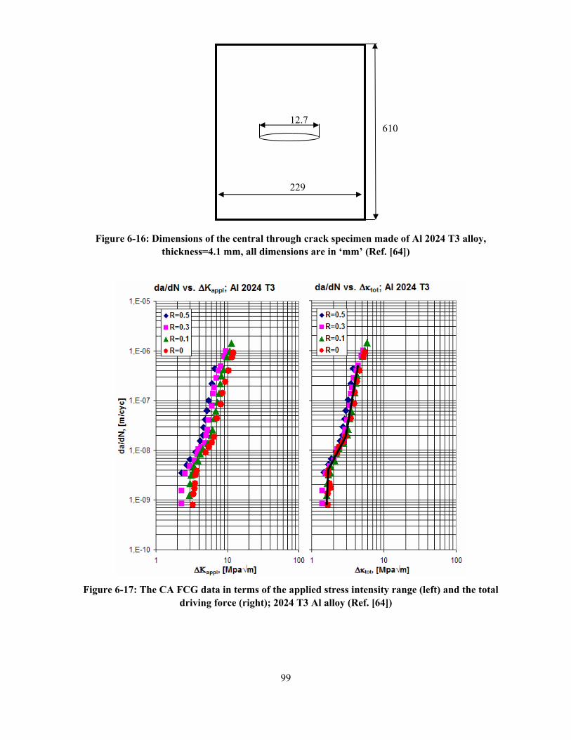
99
229
12.7610
Figure 6-16: Dimensions of the central through crack specimen made of Al 2024 T3 alloy,
thickness=4.1 mm, all dimensions are in ‘mm’ (Ref. [64])
Figure 6-17: The CA FCG data in terms of the applied stress intensity range (left) and the total
driving force (right); 2024 T3 Al alloy (Ref. [64])
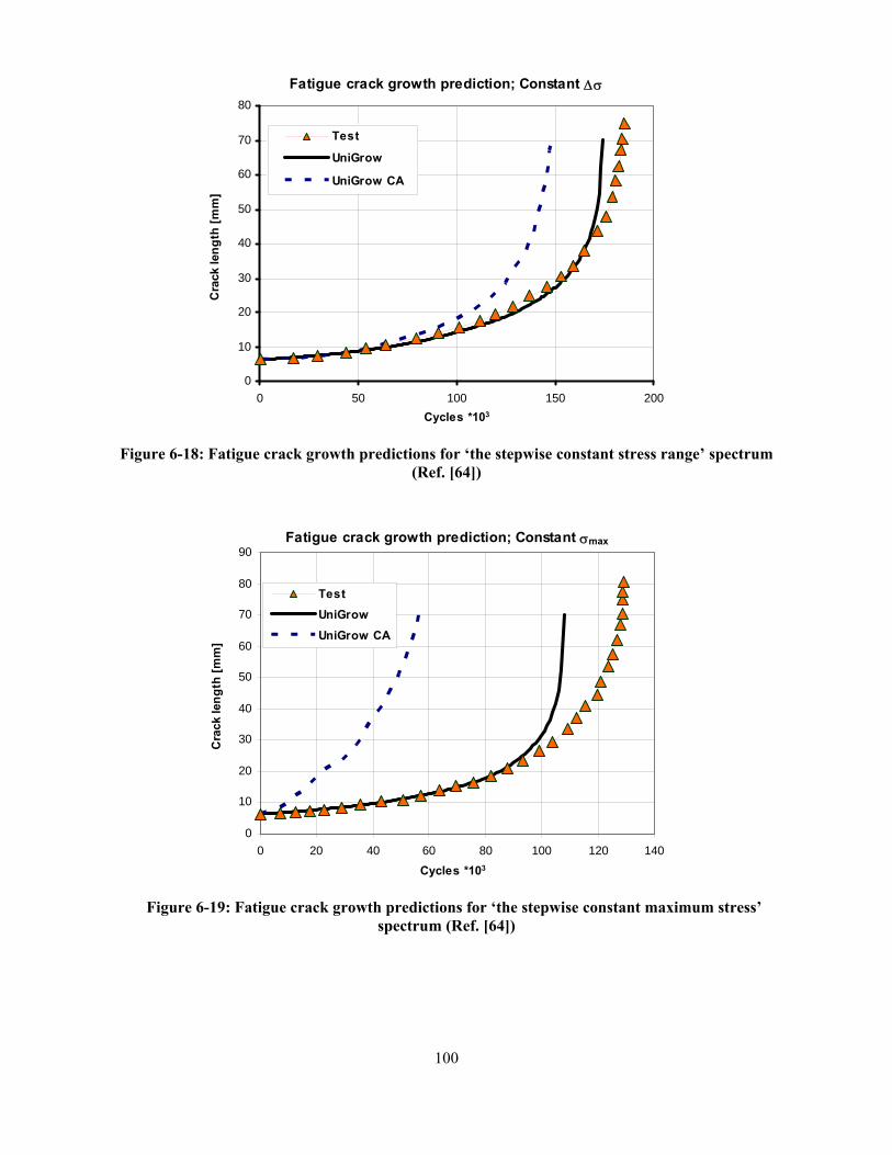
100
Fatigue crack growth prediction; Constant Δσ
0
10
20
30
40
50
60
70
80
0 50 100 150 200Cycles *103
Cra
ck le
ngth
[mm
]
Test
UniGrow
UniGrow CA
Figure 6-18: Fatigue crack growth predictions for ‘the stepwise constant stress range’ spectrum
(Ref. [64])
Fatigue crack growth prediction; Constant σmax
0
10
20
30
40
50
60
70
80
90
0 20 40 60 80 100 120 140
Cycles *103
Cra
ck le
ngth
[mm
]
TestUniGrowUniGrow CA
Figure 6-19: Fatigue crack growth predictions for ‘the stepwise constant maximum stress’
spectrum (Ref. [64])

101
6.4 Fatigue crack growth in the Al 7010 T7 alloy under constant amplitude loading spectra with overloads
The ‘Helicopter Damage Tolerance Round-Robin’ challenge was recently proposed by
Perret and Irving [65] in order to compare fatigue lives predicted by using different fatigue crack
growth approaches with those measured experimentally on the same material, in the same
component geometry and subjected to the same loading spectrum. Real helicopter material and
loading spectrum were used.
The selected geometry (used successfully in the UK ‘Round Robin’ fatigue crack growth
research project work), is a flanged plate with a central lightening hole (Figure 6-20). The
geometrical configuration is representative of many features found in a helicopter lift frame. The
initial flaw was a corner quarter-circular crack a = b = 2.0 mm located at the inner edge of the
hole. Since the specimen/crack geometry was rather complex, it was proposed that the stress
intensity vs. the crack length relationship should be the same for all participants in order to
eliminate the source of variability resulting from various SIF solutions. Therefore, the same
stress intensity factor solution based on the 3D finite element modelling was provided to all
participants of the Round-Robin challenge. However, by using the limiting values of the stress
concentration factor based on the net-cross section stress calculated by Tada et al.[66] and Raju
[67], a new stress intensity factor solution was obtained by Newman [68] for the initial crack
growth phase. A significant difference between the initial Round-Robin and Newman’s SIF
solution was found in the 2 to 5 mm crack size range. In order to verify the validity of both stress
intensity factor solutions another independent solution has been obtained by the author based on
the weight function (WF) method. It was found that as long as the crack remained quarter-
elliptical in shape the WF and Newman’s solutions were identical. However, in the transition
region (from the corner to the edge crack) Newman’s solution gives much higher stress intensity
factor than the solution for an edge crack for which the SIF should be the highest one. Therefore,

102
the combined geometry factor was used in the final analysis: the Newman/WF solution for the
corner crack stage, the edge crack solution for the transition shape, and the Irving/Newman
solution for the edge crack in the thin region of the plate (Figure 6-21). The stress intensity factor
was finally calculated as:
K S aπ β= ⋅
where the geometry factor β was obtained using the procedure described above.
The loading spectrum used in the analysis was the recently developed standard spectrum
called ASTERIX. The ASTERIX spectrum has been derived from real strain data measured on a
helicopter lift frame. The spectrum consists of data from the same 140 sorties representing 190.5
flight hours. The sequence of manoeuvres in each sortie was fixed. The total number of cycles in
its complete form is 3.67 X 10⁵ cycles. A part of the ASTERIX loading spectrum is shown in
Figure 6-22.
The round-robin component was made of Al 7010-T alloy. It is a high strength, high
toughness and stress corrosion cracking resistant aluminium alloy. The Al 7010-T7 alloy is
widely used in airspace and aircraft industries, and therefore, its properties have been already
investigated and can be easily found in literature [23] and on the internet.
Parameters of the Ramberg-Osgood and Manson-Coffin material curves were taken from the
Metallic Materials Properties Development and Standardization web-site managed by the U.S.
Department of Transportation [69] and they are listed in Table 6-5. The reference constant
amplitude fatigue growth data obtained at four different stress ratios were supplied to all
participants of ‘Helicopter Damage Tolerance Round-Robin’ challenge (Figure 6-23: (left)). The
elementary material block size, ρ*, was obtained using the third method described in Chapter 4
(Table 6-5). Based on the determined ρ* value the residual stress was determined for each

103
constant amplitude experimental da/dN data point and all experimental data points were finally
presented in terms of the total driving force resulting in one da/dN-Δκtot, ‘master curve’ shown in
Figure 6-23 (right). The single fatigue crack growth rate curve drawn in terms of the total driving
force, Δκtot, was divided into four segments and each segment was subsequently approximated
by a straight line in the log-log coordinate by using the linear regression method. Parameters of
each segment of the da/dN - Δκtot curve are listed in Table 6-5.
The experimental data, the UniGrow prediction based on Newman’s SIF solution and the
UniGrow prediction based on the combined SIF solution are shown in Figure 6-24.
In the case of Newman’s stress intensity factor solution the UniGrow fatigue crack growth
model gives results which deviate from experimental measurements. However, when the
corrected stress intensity factor solution was used, the predicted fatigue life curve (a-N) perfectly
matched the experimental data.

104
Table 6-5: Material properties of the 7010 T7 Aluminium Alloy
Constant Value Units Source E 70300 Mpa ν 0.33 σ'f 1054.5 Mpa b -0.14 ε'f 0.35 c -0.8 K' 807 MPa n' 0.09 Sys 455 MPa
Reference [69]
p 0.0825 m n’/(1+n’) ρ* 2.60E-06 Estimated using the Method 3 C1 2e-13
m1 12.294
C2 6e-11
m2 4.038
C3 9e-13
m3 7.411
C4 1e-9
m4 2.906
Fitted into the experimental CA FCG data [65] by the linear regression analysis
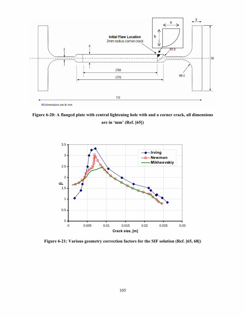
105
a
b
Figure 6-20: A flanged plate with central lightening hole with and a corner crack, all dimensions
are in ‘mm’ (Ref. [65])
0
0.5
1
1.5
2
2.5
3
3.5
0 0.005 0.01 0.015 0.02 0.025 0.03Crack size, [m]
β
IrvingNewmanMikheevskiy
Figure 6-21: Various geometry correction factors for the SIF solution (Ref. [65, 68])

106
Figure 6-22: Segment of the ASTERIX stress spectrum (Ref. [65])
Figure 6-23: CA FCG data in terms of the applied stress intensity range (left) and the total driving force (right); 7010 T7 Al alloy (Ref. [65])

107
Fatigue grack growth prediction (RR problem)
0.00
5.00
10.00
15.00
20.00
25.00
30.00
0 100 200 300 400 500
Flight hours
Cra
ck s
ize,
[mm
]Test 1Test 2UniGrow-WFUniGrow-Newman
Figure 6-24: Fatigue crack growth in the direction ‘a’ (Fig. 6-20) under the ASTERIX stress
spectrum (Ref. [65])

108
6.5 Fatigue crack growth in the Al 7075 T6 alloy specimens under P3 aircraft loading spectra
Central through crack specimens (Figure 6-25) made of Al 7075 T6 alloy were used to study
the variable amplitude fatigue crack growth behaviour. The stress intensity factor was
determined using expression:
K S a Yπ= ⋅
where :
2
1 0.5 0.32
1
a ab bY
ab
⎛ ⎞ ⎛ ⎞− +⎜ ⎟ ⎜ ⎟⎝ ⎠ ⎝ ⎠=
⎛ ⎞− ⎜ ⎟⎝ ⎠
and 2PSbt
= .
In this case ‘a’ is a half of the crack length, ‘b’ is a half of the specimen width, ‘P’ is applied
load, and ‘t’ is a thickness of the specimen.
The fatigue crack growth was analyzed for two P3 aircraft loading spectra [70]: one -
predominantly tensile loading spectrum (Figure 6-26) and the second - mixed
(tensile/compression) loading spectrum (Figure 6-27).
The Al 7075 T6 is a high strength aluminium alloy material with improved stress-corrosion
cracking resistance. Due to its high strength properties it is widely used in the following
industrial applications: aircraft fittings, gears and shafts, aerospace and defence applications.
The Ramberg-Osgood cyclic material properties were obtained from the cyclic stress-strain
experimental data provided by Jiang [71]. The experimental data and the estimated Ramberg-
Osgood curve are shown in Figure 6-28 and all constants resulted form the linear regression
fitting method are listed in Table 6-6. Two different sets of the experimental strain-life data from
Hudson [72] and Jiang [71] were put together in order to estimate parameters of the Manson-
Coffin strain-life curve (Figure 6-29, Table 6-6).

109
The reference constant amplitude fatigue growth data obtained at seven stress ratios were
provided by Jiang [71] and Newman [73] (Figure 6-30 (left)). The elementary material block
size, ρ*, was obtained using the third method described in Chapter 4 (Table 6-6). The
experimental constant amplitude fatigue crack growth data sets were presented in terms of the
total driving force, Δκtot, resulting in one ‘master curve’ shown in Figure 6-30 (right). The
‘master curve’ was divided into two segments and each segment was subsequently approximated
by a line fitted into by the linear regression method. All fitted parameters and material constants
are listed in Table 6-6.
The fatigue crack growth analysis was subsequently carried out using the UniGrow computer
program. Figure 6-31 and Figure 6-32 show the predicted UniGrow and the experimental fatigue
crack growth curves for the tension dominated and tension/compression stress spectrum.
In the first case, the applied loading spectrum was predominantly tensile and contained a
significant amount of high tensile overloads. It can be noted that the fatigue crack growth curve
obtained from the proposed model (Figure 6-31) agrees well with the experimental data. It can
also be noticed that the predicted fatigue crack growth curve is close to the experimental one not
only quantitatively but also qualitatively. One surprising observation was made that in spite of
the fact that the fatigue crack growth expression is a power law in character, both a-N curves
have the same global shape, i.e. being close to a straight line. This effect comes from the fact that
the residual minimum stress field was created mostly by stresses induced by high overload
cycles. Therefore the instantaneous residual stress intensity factor was dependent mostly on these
overloads which were reducing the total driving force as the crack was increasing making it
almost independent of the crack length, i.e. the average total driving force was almost constant
during the crack growth period.

110
In the second case, the applied loading spectrum was approximately half tensile and half
compressive, with no high overloads. However, the amount of compressive under-loads was
significant and resulted in the reduction of compressive residual stresses. As the experimental
measurements and predicted results indicate, the fatigue life for the second loading spectrum was
shorter than for the first one. Also, in the second case, the fatigue crack growth curve a-N curve
has the right shape as suggested by the power law fatigue crack growth expression. It can be
explained by the fact that the fatigue crack growth was not interrupted by the retardation effect
induced by high overloads because it was balanced out by the relaxation effect of under-loads.

111
Table 6-6: Material properties of the 7075 T6 Aluminium Alloy
Constant Value Units Source E 71000 MPa ν 0.33 σ'f 778.6 MPa b -0.0629 ε'f 0.2387 c -0.6944 K' 864.1 MPa n' 0.0866 Sys 66 MPa
Hudson [72], Jiang [71]
p 0.0797 n’/(1+n’) ρ* 4.4e-6 m Estimated using the Method 3 C1 8e-18
m1 30.05
C2 2e-10
m2 3.42
Fitted into the experimental CA FCG data [71,73] by the linear regression analysis

112
Figure 6-25: Central through crack specimen made of Al7075 T6 alloy (Ref. [70])
Figure 6-26: Predominantly tensile P3 stress spectrum; Al 7075 T6 alloy (Ref. [70])
Figure 6-27: Compressive/tensile P3 stress spectrum; Al 7075 T6 alloy (Ref. [70])

113
Figure 6-28: Experimental data and the fitted cyclic stress – strain curve (Ref. [71,72])
1.E-03
1.E-02
1.E-01
1.E+00
1.E+00 1.E+01 1.E+02 1.E+03 1.E+04 1.E+05 1.E+06 1.E+07
Number of reversal, 2Nf.
Tota
l Str
ain
Am
plitu
de, Δ
ε/2. Coffin-Manson
JiangExp. data
Figure 6-29: The Manson-Coffin fatigue curve; Al 7075 T6 alloy (Ref. [71, 73])

114
Figure 6-30: CA FCG data in terms of the applied stress intensity range (left) and the total driving
force (right); 7075 T6 Al alloy (Ref. [71, 73])

115
Figure 6-31: The predicted fatigue crack growth curve and experimental data for the
predominantly tensile spectrum (Ref. [70])
Figure 6-32: The predicted fatigue crack growth curve and experimental data for the
tensile/compressive stress spectrum (Ref. [70])

116
6.6 Fatigue crack growth in the Al 7050-T7 alloy under the F/A-18 aircraft loading spectrum
Another verification of the UniGrow fatigue crack growth model has been performed using
the Al 7050-T7451 alloy in order to investigate the fatigue crack growth in the F/A-18 aircraft.
The experimental fatigue crack growth data were supplied by the Australian Defence Science
and Technology Organisation [74]. In this case the semi-elliptical crack in the wing attachment
carry-through bulkhead (Figure 6-33) was monitored. The initial crack size detected and later
monitored on the surface was 3 microns. The stress intensity factor was determined using the
expression of Newman [75]
K S b Yπ= ⋅
where : ( )
, , 'sb b aFa t WY
E k
ϕ⎛ ⎞⎜ ⎟⎝ ⎠= .
In this case Fs is a function of crack length ‘a’, crack depth ‘b’, specimen thickness ‘t’, specimen
width ‘W’, and angle ‘φ' which defines the point along the crack front (Figure 6-33). E(k) is an
elliptical integral of the second kind.
The Mini FALSTAF loading spectrum provided by the Australian Defence Science and
Technology Organisation [74] was used in the experimental fatigue crack growth analysis. The
applied loading spectrum was predominantly tensile and contained both overload and under-load
(Figure 6-34) cycles.
The Al 7050-T7451 alloy has a very high strength coupled with high resistance to corrosion
and stress-corrosion cracking, high fracture toughness, and good fatigue resistance. Similarly to
the Al 7010 T73651 alloy analyzed in Section 6.4, it is widely used in aircraft industry, and
therefore, its properties have been already studied and can be found in the internet. The same

117
web-site managed by the U.S. Department of Transportation [69] provides the Ramberg-Osgood
and Manson-Coffin material properties (Table 6-7) for the material being studied. The reference
constant amplitude fatigue growth data sets obtained at three different stress ratios were taken
from the paper by Sharp [76] (Figure 6-35 (left)). The elementary material block size, ρ*, was
obtained using the third method described in Chapter 4 (Table 6-7). Based on the determined ρ*
value the residual stress was determined for each experimental constant amplitude da/dN data
point and then all experimental data points were presented in terms of the total driving force
resulting in one, da/dN-Δκtot, master curve as shown in Figure 6-35 (right). The resulting single
fatigue crack growth rate curve, drawn in terms of the total driving force Δκtot, was divided into
two segments and each segment was subsequently approximated by a line fitted into by the linear
regression method. All fitted parameters and material constants are listed in Table 6-7.
The comparison between the predicted and experimental fatigue crack growth data shows the
capability of the UniGrow fatigue crack growth model to predict fatigue growth of very small
cracks and fatigue lives of components with such small cracks (Figure 6-36).

118
Table 6-7: Material properties of the 7050 T7451 Aluminum Alloy
Constant Value Units Source E 71016 MPa ν 0.33 σ'f 639.14 MPa b -0.08 ε'f 0.3598 c -0.914 K' 704 MPa n' 0.0706
Reference [69]
p 0.0659 n’/(1+n’) ρ* 2e-5 m Estimated using the Method 3 C1 4e-11 m1 4.46
C2 1e-10
m2 3.72
Fitted into the experimental CA FCG data [76] by the linear regression analysis

119
2a
b φ t
Figure 6-33: The component and crack macrographs; Al 7050-T7451 alloy (Ref. [74])
F/A-18 aircraft
-200
-100
0
100
200
300
400
500
0 2000 4000 6000 8000 10000 12000 14000 16000 18000
Cycles
App
lied
load
, MPa
Figure 6-34: The F/A-18 aircraft tensile loading spectrum (Ref. [74])

120
Figure 6-35: CA FCG data in terms of the applied stress intensity range (left) and the total driving force (right); 7050 T7 Al alloy (Ref. [76])

121
Fatigue life prediction; AL 7050 T7
0.001
0.01
0.1
1
10
0 100000 200000 300000 400000 500000 600000 700000
Cycles
Cra
ck le
ngth
, mm
Test data
UniGrow
Figure 6-36: The Fatigue crack growth prediction and experimental data for the F/A-18 aircraft
loading spectrum in the direction ‘a’ (Ref. [74])

122
6.7 Fatigue crack growth in the AL 2324-T3 alloy under the P3 aircraft loading spectrum
In order to understand the variable amplitude loading effects on fatigue crack growth and
simultaneously to verify the UniGrow fatigue crack growth model four sets of experiments were
performed by Kujawski [77].
Edge crack specimens made of Al 2324 T3 alloy (Figure 6-37) were used in order to generate
the fatigue crack growth data. It has to be mentioned that the specimens were not the classical
specimens with an uniformly distributed stresses along its remote edges. In this case uniformly
distributed displacements were applied along edges of the specimen. The stress intensity factor
solution for this particular case was developed by Newman [78] and it is given below.
K S a Yπ= ⋅
where:2 3 4 5
1.122 0.51 7.73 32.32 45.37 23.72a a a a aW W W W W
⎛ ⎞ ⎛ ⎞ ⎛ ⎞ ⎛ ⎞ ⎛ ⎞= − − + − +⎜ ⎟ ⎜ ⎟ ⎜ ⎟ ⎜ ⎟ ⎜ ⎟⎝ ⎠ ⎝ ⎠ ⎝ ⎠ ⎝ ⎠ ⎝ ⎠
Y and PStW
= .
In this case ‘a’ is the crack length, ‘W’ is the specimen width, ‘t’ is the specimen thickness, and
‘P’ is applied load.
The fatigue crack growth was studied experimentally first in specimens subjected to the
tensile/compressive P3 aircraft loading spectrum (Figure 6-38). In the next sets of experiments
the compressive part of the spectrum was removed (Figure 6-39). Therefore, comparison of the
fatigue crack growth data obtained under the original and the tensile only loading spectra allows
estimating the influence of the compressive part of the loading history on the fatigue crack
growth.
In the next step of Kujawski’s experimental research activities the upper part of the positive
loading spectrum was cut off at 95%, 85%, and 65% load level relative to the highest stress peak

123
in the entire spectrum. In other words, only a few high overloads were reduced to the 95% stress
level in the first case, the high and medium stress cycles reduced in the second case, and almost
all above average stress cycles were reduced to 65% in the third case (Figure 6-40). The
retardation effect of multiple overloads can be quantified by comparing the fatigue lives
corresponding to these truncated loading spectra with that one corresponding to the original
tensile only loading spectrum. This type of analysis is similar to the one described in Section 6.2
(single overload retardation effect). However, the current analysis takes into account not only the
retardation effect due to the large residual stress fields produced by overloads but also the
counteractive acceleration effect caused by the presence of high number of overloads with high
stress ranges which themselves directly contribute to the crack propagation. The truncation of the
loading spectrum from the top reduces the residual stresses produced by overloads but also
eliminates cycles with high stress intensity ranges and high maxima which significantly
contribute to the fatigue crack propagation. Thus, it is interesting to see which effect may
dominate.
The same idea but approached from a different point of view was studied while carrying out
the third set of experiments. The original loading spectrum was scaled in the third case by a
factor of 0.95, 0.85, and 0.65 respectively. Scaling the loading spectrum brings the same effect as
previously due to reduced residual stresses and decrease of the crack growth rate due to reduced
driving force.
In the last set of experiments the fatigue crack growth was monitored under combined
truncated and scaled loading spectra.
The experimental cyclic stress/strain material properties were provided by Kujawski in
reference [77] and they are listed in Table 6-9. Unfortunately, the Manson-Coffin strain – life
fatigue data for the Al 2324 T3 alloy was unknown, and therefore, the fatigue crack growth

124
analysis was performed based on the constant amplitude fatigue crack growth data only. The
constant amplitude fatigue crack growth data obtained at four different stress ratios (Figure 6-41
(left)) was also provided by Kujawski [77]. Due to the nature of available material data the
second method, described in Chapter 4, was used to estimate the elementary material block size,
ρ*, listed in Table 6-9. All experimental constant amplitude fatigue crack growth data points
were plotted in terms of the total driving force, Δκtot, resulting in one ‘master’ curve as shown in
Figure 6-41 (right). The ‘master’ curve was divided into two segments and subsequently
approximated by two linear pieces in the log-log scale by using the linear regression method. All
fitted parameters and material constants are listed in Table 6-9.
The following Table 6-8 contains detailed description of all loading spectra used in the
experiments and subsequent numerical modeling as well as experimental fatigue lives in absolute
and relative terms, predicted fatigue lives and the prediction error. Negative sign in ‘Prediction
error’ column means that the prediction was conservative.
Table 6-8: Spectra description and fatigue life predictions for AL 2324 T7
Spectrum name Maximum Applied
Load
Minimum Applied
load
Average Exper.
Fatigue life [Cycles]
Average Exper. relative
Fatigue life
Predicted Fatigue life
[Cycles]
Prediction Differ.

125
(kN) (kN) [Cycles]
Original spectrum 18 -9 1680000 1 1510000 -10.1%
Tensile spectrum 18 0 5636000 3.355 4130000 -26.7%
Tensile/Truncated 95% 17.1 0 4850000 2.886 4300000 -11.3%
Tensile/Truncated 85% 15.3 0 1988000 1.183 1950000 -1.9%
Tensile/Truncated 65% 11.7 0 935800 0.557 1070000 +14.3%
Original/Scaled 85% 15.3 -7.65 2819000 1.678 2600000 -7.8%
Original/Scaled 65% 11.7 -5.85 5922000 3.525 5500000 -7.1%
Original/Scaled/Truncated 85% 13 -7.65 1965000 1.170 1760000 -10.4%
Tensile/Scaled/Truncated 85% 13 0 4348000 2.588 3900000 -10.3%
The predicted and experimental crack length vs. number of cycles (a-N) data sets for the
original P3 aircraft loading spectrum are shown in Figure 6-42. The predicted final fatigue life
corresponding to the crack length of a=35 mm was conservative by approximately 10%.
In the case of the tensile only loading spectrum the fatigue life (Figure 6-42) was 3.355 times
longer than that one obtained under the original loading spectrum. This result could be
anticipated due to the fact that compressive part of the cycle does not contribute too much to the
fatigue crack growth itself but it may eliminate the retardation effect of high overload cycles. In
other words, in the case of the tensile loading spectrum (no underloads) the residual stress
retardation effect was much greater than in the original case. The relative error of the UniGrow
fatigue life prediction was the highest in this particular case (ca. 26%).

126
The cutting off operation of the tensile loading spectrum at 95% load level has reduced the
fatigue life by around 14% while compared to the original tensile only stress spectrum. It means
that mostly the high overloads are responsible for the retardation effect resulting from residual
stresses and but they do not bring much contribution to the overall total driving force. The
predicted fatigue life in this case was close to the experimental one (-11% difference) and both a-
N curves are shown in Figure 6-43.
The same trend was observed for two other truncated spectra. Subsequent truncation of the
loading spectra at 85% and 65% load level reduced the fatigue life corresponding to the crack
length of a=35 mm by approximately 2.8 and 6 times respectively (Figure 6-43). It is interesting
to note that the fatigue life of the 65% truncated tensile loading spectrum was shorter than that
one corresponding to the original tensile spectrum. This can be explained by the fact that the
truncation of the upper part of the loading spectrum does not affect the prevailing number of so-
called ‘small’ cycles which have the strongest overall influence on the fatigue crack growth. The
UniGrow fatigue crack growth model was in both cases capable to simulate correctly the
acceleration effect of the truncation of the loading spectrum. The relative error of the UniGrow
prediction for the 85% truncated spectrum is was only 2% and for the 65% truncated spectrum is
was around 14%.
The opposite effect was observed in the case of the original versus scaled loading spectra.
Despite of the fact that scaling of the original spectrum reduced the amount of residual stresses in
the crack tip region it also reduce the total fatigue driving force for each cycle causing the major
retardation of the fatigue crack growth. Loading spectra scaled by the coefficients 0.85 and 0.65
yielded fatigue lives 1.7 and 3.5 times longer than original one (Figure 6-44). In both cases the
fatigue crack growth prediction based on the UniGrow model agrees well with the experimental
data and the relative error was less than 10%.

127
The last case combines both the acceleration effect of the truncation and the retardation effect
of the scaling. The 85% truncation and 85% scaling operations were simultaneously applied to
both the original compressive-tensile and the tensile only loading spectra. As it was expected the
acceleration and the retardation effect cancelled out each other and the final fatigue life did not
change much (Figure 6-45) when compared with appropriate original spectra. The predicted
UniGrow fatigue crack growth simulates very well the experimental data and the relative error
was around 10% for both cases.

128
Table 6-9: Material properties of the 2324 T7 Aluminums Alloy
Constant Value Units Source E 72407 MPa ν 0.33 K' 877.5 MPa n' 0.14
Kujawski [77]
p 0.12 n’/(1+n’) ρ* 1.5e-5 m Estimated using Method 2 C1 4e-11 2e-18 m1 4.46 29.381 C2 1e-10 1e-11 m2 3.72 5.08
Fitted into the experimental CA FCG data by [77] the linear regression analysis

129
6.35 mm
R=7 mm
t=2.54 or 5.08 mm
6.35 mm
R=7 mm
t=2.54 or 5.08 mm
Load
45 mm
2 mm
37 mm
50 mm
25 mm125 m
m
Hydraulic gripping
45o
45 mm
Figure 6-37: Dimensions of the edge crack specimen made of the Al 2324 alloy (Ref. [77])

130
Figure 6-38: The original compression-tensile loading spectrum for the P3 aircraft (Ref. [77])
Figure 6-39: The tensile only loading spectrum for the P3 aircraft (Ref. [77])
Figure 6-40: Truncated loading spectra obtained from the P3 aircraft tensile only loading spectrum
(Ref. [77])
95% 85% 65%
128869Points
Load
Compressive loads deleted
128869Points
Load
128869Points
Load

131
Figure 6-41: Fatigue crack growth rate in terms of the applied stress intensity range (left) and the total two-parameters driving force (right); Al 2324 (Ref. [77])

132
FCG prediction (original compression-tensile and tensile only spectra)
0
5
10
15
20
25
30
35
40
45
0 1000000 2000000 3000000 4000000 5000000 6000000 7000000
N,[Cycles]
a, [m
m]
Original compression-tensile, test 1Original compression-tensile, test 2Original compression-tensile, test 3Original compression-tensile, UniGrowOriginal tensile only, test 1 Original tensile only, test 2 Original tensile only, test 3 Original tensile only, UniGrow
Figure 6-42: FCG predictions and experiments (original compression-tensile P3 vs. original tensile
only P3) (Ref. [77])

133
FCG prediction (truncated tensile only loading spectra)
0
5
10
15
20
25
30
35
40
45
0 1000000 2000000 3000000 4000000 5000000 6000000 7000000
N,[Cycles]
a, [m
m]
Tensile only, truncation 65%, test Tensile only, truncation 85%, test Tensile only, truncation 95%, test Original tensile only, test 3Original tensile only, UniGrowTensile only, truncation 65%, UniGrow Tensile only, truncation 85%, UniGrow Tensile only, truncation 95%, UniGrow
Figure 6-43: FCG predictions and experiments (truncated tensile only loading spectra) (Ref. [77])

134
FCG prediction (scaled original compression-tensile loading spectra)
0
5
10
15
20
25
30
35
40
45
0 1000000 2000000 3000000 4000000 5000000 6000000 7000000
N,[Cycles]
a, [m
m]
Original compression-tensile, scaled 85%, UniGrowOriginal compression-tensile, scaled 65%, UniGrowOriginal compression-tensile, scaled 85%, testOriginal compression-tensile, scaled 65%, test
Figure 6-44: FCG predictions and experiments (scaled original compression-tensile loading spectra)
(Ref. [77])

135
FCG prediction (scaled and truncated loading spectra)
0
5
10
15
20
25
30
35
40
0.E+00 5.E+05 1.E+06 2.E+06 2.E+06 3.E+06 3.E+06 4.E+06 4.E+06 5.E+06 5.E+06
N,[Cycles]
a, [m
m]
Original compression-tensile, Sc. and Tr. 85%, testOriginal tensile only, Sc. and Tr. 85%, testOriginal compression-tensile, Sc. and Tr. 85%, UniGrowOriginal tensile only, Sc. and Tr. 85%, UniGrow
Figure 6-45: FCG predictions and experiments (scaled and truncated original compression-tensile
and tensile only loading spectra) (Ref. [77])

136
Chapter 7 Conclusions and Future Recommendations
A two-parameter fatigue crack growth model derived initially for constant amplitude cyclic
loading histories has been extended and modified in order to account for variable amplitude
loading effects. This goal has been accomplished through careful investigation of experimental
fatigue crack growth data under a variety of variable amplitude loading spectra.
It has been shown that various effects on fatigue crack growth resulting from the application
of cyclic variable amplitude loading may be modeled by accounting for the residual stresses
caused by reversed cyclic plastic deformation in the crack tip region. An elastic-plastic stress-
strain analysis and five memory rules are needed for the determination of the residual stress field
in the crack tip region. The analysis needs to be carried out on the cycle-by-cycle basis
accounting for the load/stress history effects. It has been shown that the use of ‘memory rules’
and the two-parameter driving force enables accurate prediction of fatigue lives of cracked
bodies subjected to complex variable amplitude service loading spectra.
The UniGrow fatigue crack growth model and the entire methodology has been programmed
into the UniGrow fatigue crack growth analysis computer software package making the method
usable to other parties. The software can carry out fatigue crack growth analyses for a variety of
geometrical configurations with one and two-dimensional cracks under the application of
arbitrary variable amplitude loading spectrum.
Several recommendations can be made concerning future research in the field of fatigue
crack growth analysis in general, and the UniGrow fatigue crack growth model in particular.
An accurate and efficient method for determining strains and stresses in the crack tip region
is required for fatigue crack growth analyses. The UniGrow fatigue crack growth model uses for

137
that purpose the improved and extended Neuber rule. However, it is important to keep in mind
that this is an approximation. Stresses and strains estimated with the help of the Neuber rule are
in general reasonably accurate but conservative and limited to plane stress or plane strain state.
Despite the fact that the error is relatively small, the fact is that it can be accumulated through the
entire loading history and it may at the end result in the overestimation of the fatigue crack
growth rate. Therefore, combination of the UniGrow fatigue crack growth model with a non-
linear finite element analysis can improve the fatigue crack growth prediction. The idea of using
finite element method was initially abandoned due to high demand concerning the computational
time needed for the analysis. However new computers may make such a task feasible.
The advantage of using the FE method combined with the UniGrow model lies in the fact that it
would make it possible to analyse arbitrary cracks without the necessity of calculating stress
intensity factors. Such an approach would make it possible to analyse natural cracks without the
necessity of approximating them by any regular geometrical figures (such as ellipses) and to
apply any type of cyclic variable amplitude loading spectra.

138
Appendix The UniGrow Fatigue Crack Growth Software
Considering all methods, equations, and rules described in previous chapters; it becomes
clear that a special computational algorithm is required in order to implement the UniGrow
fatigue crack growth model.
It could be said that the first parts of the UniGrow software were created around 20 years ago
by Glinka and Buczynski. They developed a set of separate programs for the elastic-plastic
stress/strain determination based on the Neuber rule (NMPH), for the SIF estimation based on
the weight function technique for any provided stress distribution (WF), and for the fatigue life
analysis under constant and variable amplitude loading (FALPR). However, the effect of residual
stresses on the FCG was not accounted for since the appropriate algorithm has not been
developed yet.
The first version of UniGrow software (UniGrow 1.0) was a routine developed using C++
programming language (Borland Builder C++ 6.0 platform) in order to connect all the programs
described above and include the residual stress effect. Moreover, a set of algorithms has been
developed in order to implement the five ‘memory’ rules described in Chapter 5. These
algorithms have been later modified in order to decrease the computational time required for the
FCG analysis. Additionally, it has been found that calling several separate programs developed
based on the different programming languages for each cycle of a variable amplitude loading is
too time consuming.
Therefore, main algorithms from NPMH, WF, FALPR, and UniGrow 1.0 itself were
modified and rewritten in C.net platform using ZedGraph graphical library resulting in the
UniGrow .Net version for Windows XP/Vista. This decreased the computational time and

139
allowed to create the basic user interface with a choice of specimen/crack configurations and
material library. Most of the fatigue crack growth predictions described in the Chapter 6 were
obtained using ‘.net’ version of the UniGrow software.
Recently, due to the sponsor’s request, ‘.net’ platform has been changed to Qt cross-platform
application development framework and both Windows and Linux versions have been released.
The UniGrow Qt version has a very friendly user interface and a large choice of the
specimen/crack geometries and material constants.
The following list briefly describes the main algorithm of the UniGrow Qt software not
including the interface feathers and ‘build in’ load editor.
Before the FCG analysis:
1. Check the supplied loading spectrum: it should not have any consequent peaks or valleys or
fully negative cycles. Otherwise, user will be notified that the loading spectrum has been
automatically corrected.
2. Check the supplied material data: all material constants required for the FCG analysis have
to be specified. Otherwise, user will be asked to re-enter them.
3. Check crack configuration and component geometry: all the dimensions required for the
FCG analysis have to be specified and should not contradict each other. Otherwise, user will
be asked to re-enter them.
4. Reserve computer memory for the resultant residual stress filed which will be accumulated
through the loading history based on the ‘memory’ rules.
For each cycle of the loading history (step ‘i’)

140
1. Determine the applied maximum SIF and SI range based on Eq. 2-3
2. Use the residual SIF obtained during the previous (i-1) step to calculate the total maximum
SIF and the SI range based on Eq. 3-12 and Eq. 3-13.
3. Find the crack increment due to the first loading reversal based on Eq. 3-28
4. Determine the residual stress destitution ahead of the crack tip induced by the current
loading cycle based on Eq. 3-7, Eq 3-8, and Eq. 3-9.
5. Use the first ‘memory’ rule.
6. Use the second ‘memory’ rule (if needed).
7. Use the third ‘memory’ rule (if needed).
8. Use the fourth ‘memory’ rule (if needed).
9. Use the fifth ‘memory’ rule (if needed).
10. Modify the resultant residual stress field produced through the preceding loading history
based on five memory rules.
11. Calculate the new value of the instantaneous residual SIF based on Eq. 3-11.
12. Check whenever the following cycle can cause the memory overflow. Reserve additional
memory if needed.
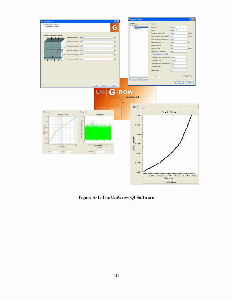
141
Figure A-1: The UniGrow Qt Software

142
Bibliography
[1] N.E. Dowling, Mechanical behavior of materials, New-Jersey, Prentice-Hall, 1993
[2] A.H. Noroozi., G. Glinka., S. Lambert, A study of the stress ratio effects on fatigue crack
growth using the unified two-parameters fatigue crack growth driving force, International
Journal of Fatigue, 2007, Vol. 29, 1616-1634.
[3] A. A. Griffith, The Phenomena of Rapture and Flow in Solids, Philos. Trans., R. Soc. Lond.,
Ser. A., 1920, Vol. 221, p. 163.
[4 ] G. R. Irwin, Analysis of Stresses and Strains Near the And of a Crack Traversing a Plate, J.
Appl. Mech., 1957, Vol. 24, p. 361.
[5] H.M. Westergaard, Journal of Applied Mechanics, Transactions of the American Society of
Mechanical Engineers, 1939, A49–A53.
[6] M. Creager, P.C. Paris, Elastic field equations for blunt cracks with reference to stress
corrosion cracking, Int. J. Fracture, 1967, Vol. 3, pp. 247–251.
[7] P.C. Paris, M.P. Gomez, W.E. Anderson, A rational analytic theory in fatigue, The Trend of
Engineering, 1961, Vol. 13-1, pp. 9-14.
[8] R.G. Forman, V.E. Kearney, R.M. Engle, Journal of Basic Engineering, 1967, Vol. 89, pp.
459–464.
[9] D. Broek, The Practical Use of Fracture Mechanics, Kluwer Academic Publishers, 1989.
[10] J. Weertman, Rate of Growth of Fatigue Cracks Calculated from the Theory of Infinitesimal
Dislocations Distributed on Plane, International Journal of Fracture Mechanics, 1966, Vol. 2,
pp. 460-467.

143
effK
[11] T.L. Anderson, Fracture mechanics: fundamentals and applications (2nd ed), CRC Press,
West Palm Beach, FL, 1995.
[12] H. Suzuki, A. McEvily, Metall. Trans., 1979, 10A, 475–81.
[13] E.K. Walker, The effect of stress ratio during crack propagation and fatigue for 2024-T3 and
7076-T6 aluminium, Effect of Environment and Complex Load History on Fatigue Life, ASTM
STP 462, Philadelphia: American Society for Testing and Materials, 1970, pp.1-14.
[14] K. Donald, P.C. Paris, An evaluation of Δ estimation procedure on 6061-T6 and 2024-
T3 aluminum alloys, International Journal of Fatigue, 1999, Vol. 21, pp. S47-S57.
[15] A.K.Vasudevan, K. Sadananda, N. Louat, A review of crack closure, fatigue crack threshold
and related phenomena, Material Science and Engineering, 1994, Vol. A188, pp. 1-22.
[16] W. Elber, Fatigue Crack Closure under Cyclic Tension, Engineering Fracture Mechanics,
1970, Vol. 2, pp. 37-45.
[17] S. Suresh, Fatigue of Metals, Cambridge University Press, Cambridge,1991
[18] D.E. Macha, D.M. Corby, J.W. Jones, On the variation of fatigue-crack-opening load with
measurement location, Experimental Mechanics, 1979, Vol. 19, No.6, pp.207-213.
[19] M.R. Ling, J. Schijve, The effect of the intermediate heat treatments and overload induced
retardation during fatigue crack growth in Al-Alloy, Fracture of Engineering Materials and
Structures, 1992, Vol. 15, pp. 421-430,
[20] G.G. Garrett, J.F. Knott, On the effect of crack closure on the rate of fatigue propagation,
International Journal of Fracture, 1977, Vol. 13, pp 101-104.

144
[21] L.W. Wei, N.M. James, A study of fatigue crack closure in polycarbonate CT specimens,
Engineering Fracture Mechanics, 2000, Vol. 66, pp 223-242.
[22] N. Louat, K. Sadananda, M. Duesberry, A.K. Vasudevan, A Theoretical Evaluation of
Crack Closure, Metallurgical Transactions, 1993, Vol. 24A, pp. 2225-2232.
[23 ] R.I. Stephens, A. Fatemi, R.R. Stephens, H.O. Fuchs, Metal Fatigue in Engineering, Published by Wiley & Sons, Inc., 2000, ISBN 0-471-51059-9. [24] R.H. Christensen, Fatigue crack, fatigue damage and their directions, Metal Fatigue,
McGraw-Hill, New York, 1959.
[25] N.A. Fleck, Influence of stress state on crack growth retardation, Basic Questions on
Fatigue, 1988, Vol. 1, ASTM STP 924, pp. 157-183.
[26] N.A. Fleck, Fatigue crack growth due to periodic underloads and overloads, Acta Metall.
1985, Vol. 33, pp. 1339-1354.
[27] J. Schijve, D. Broek, The result of a test programme based on a gust spectrum with variable
amplitude loading, Aircraft Engineering, Vol. 34, pp. 314-316.
[28] M. Croft, Private communications
[29] O.E. Wheeler, Spectrum loading and crack growth, Journal of Basic Engineering, 1972 Vol.
94, pp. 181-186.
[30] J. Willenborg, R.M. Engle, H.A. Wood, A crack growth retardation model using an
effective stress concept, Report # AFFDL-TR71-1, Air Force Flight Dynamic Laboratory,
Wright-Patterson Air Force Base, USA, 1971.
145
[31] S.L. Ouk, Zhi Wei Chen, Improvement to Crack Retardation Models Using"Interactive
Zone Concept", International Journal of the Korean Society of Precision Engineering, 2002,
Vol. 3-4.
[32] U.H. Padmadinata, Investigation of crack-closure prediction models for fatigue in
aluminum alloy sheet under flight-simulating loading, PhD – thesis, Delft University of
Technology, Faculty of Aerospace Engineering, 1990.
[33] J.C Newman, Prediction of fatigue crack growth under variable amplitude and spectrum
loading using a closure model, ASTM STP 761, American Society for testing and materials,
Philadelphia, pp. 255-277, 1982.
[34] S. Suresh, Fatigue of Materials, Cambridge University Press, Cambridge, 1991.
[35] J. Bannantine, Fundamentals of Metal Fatigue Analysis, Prentice-Hall Inc., USA, 1990.
[36] R.W. Landgraf, J. Morrow, T. Endo, Determination of the cyclic stress-strain curve, Journal
of Materials, 1969, Vol. 4, No. 1, pp. 176.
[37] Technical Report on Low Cycle Fatigue Properties: Ferrous and Non-ferrous Metals, SAE
Standard No. J1099, Society of Automotive Engineers (SAE), Warrendale, Pennsylvania, 1998.
[38] K.N. Smith, P. Watson, T.H. Topper, A stress-strain function for the fatigue of metals,
Journal of Materials, 1970, Vol. 5, No. 4, pp. 767-778.
[39] A. Noroozi, Development of a two-parameter model for fatigue crack growth analysis, PhD
thesis, Department of Mechanical Engineering, University of Waterloo, Waterloo, 2007.
[40] H. Neuber, Theory of stress concentration for shear-strained prismatic bodies with arbitrary
nonlinear stress-strain law, ASME Journal of Applied Mechanics, 1961, Vol. 28, pp. 544-551.

146
[41] G. Glinka, A notch stress-strain analysis approach to fatigue crack growth, Engineering
Fracture Mechanics, 1985, Vol. 21, No. 2, pp.245-261.
[42] P.J.E. Forsyth, Unified description of micro and macroscopic fatigue crack behaviour,
International Journal of Fracture, 1983, Vol. 5, pp. 3-14.
[43] A. Moftakhar, A. Buczynski, G. Glinka, Calculation of elastoplastic strains and stresses in
notched under multiaxial loading, International Journal of Fracture, 1995, Vol. 70, No. 3, pp.
357-373.
[44] G. Glinka, A. Buczynski, Multiaxial stress-strain notch analysis, Multiaxial Fatigue and
Deformation, editors: Kalluri S, et al. ASTM STP 1387, Philadelphia, American Society for
Testing and Materials, pp. 82-98, 2000.
[45] Z. Zeng, A. Fatemi, Elasto-Plastic Stress and Strain Behavior at Notch Roots Under
Monotonic and Cyclic Loadings, Journal of Strain Analysis, 2001, Vol. 36, No. 3, pp. 287-300.
[46]J.J Skrzypek, R.B. Hetnarski, Plasticity and Creep: Theory, Examples and Problems, CRC
Press, Boca Raton, 1993.
[47] G. Glinka, G. Shen , Universal features of weight functions for cracks in mode I,
Engineering Fracture Mechanics, 1991, Vol. 40, No. 6, pp. 1135-1146.
[48] G. Shen, G. Glinka, Determination of weight functions from reference stress intensity
factor, Theoretical and Applied Fracture Mechanics, 1991, Vol. 15, No. 3, pp. 237-245.
[49] X. Wang, S. Lambert, G. Glinka, Approximate weight functions for embedded elliptical
cracks, Engineering Fracture Mechanics, 1998, Vol. 59, No.3, pp. 381-392.
[50] A. Moftakhar, G. Glinka, Calculation of stress intensity factors by efficient integration of
weight functions, Engineering Fracture Mechanics, 1992, Vol. 43, No. 5, pp.749-756.
147
[51] H. Kitagawa, S. Takahashi: Applicability of Fracture Mechanics to Very Small Cracks in
the Early Stage, Proceedings of the Second International Conference on Mechanical Behavior of
Materials, American Society for Metals, Metals Park, 1976, pp. 627-631.
[52] A.K. Vasudevan, K. Sadananda, N. Louat, Reconsideration of Fatigue Crack Closure,
Scripta Metallurgica et Materialia, 1992, Vol. 27, pp. 1673-1678.
[53] M. Skorupa, Load interaction effects during fatigue crack growth under variable amplitude
loading – Literature review, Part II: qualitative interpretation, University of Mining and
Metallurgy, Al. Mickiewicza 30, 30-059 Krakow, Poland, 1998.
[54] American Society for Testing and Materials, ASTM E606-92 Standard practice for strain
controlled fatigue testing, ASTM, Philadelphia (1992)
[55 ] A. Fatemi, A. Plaseieda, A.K. Khosrovanehb, D. Tanner, Application of bi-linear log–log
S–N model to strain-controlled fatigue data of aluminum alloys and its effect on life predictions,
International Journal of Fatigue, 2005, Vol. 27-9, pp. 1040-1050.
[56] J. Schijve, Observations on the Prediction of Fatigue Crack Growth Propagation Under
Variable-Amplitude Loading, Fatigue Crack Growth Under Spectrum Loading, ASTM STP 595,
American Society for Testing and Materials, Philadelphia, PA, 1976, pp. 3-23.
[57] S.M. Russ, Effect of underloads on fatigue crack growth of Ti-17. Ph.D. Thesis, Materials
Science and Engineering Department, Georgia Institute of Technology, Atlanta, GA, USA,
October 2003.
[58] G.R Chanani, Retardation of fatigue crack growth in 7075 Aluminum, Metals Engineering
Quarterly, 1975, Vol. 15, No. 1, pp. 40-48.
[59] F.J. McMaster, Smith D. J., Prediction of fatigue crack growth in aluminum alloy 2024-
T351 using constraint factors, International Journal of Fatigue, 2001, Vol. 23, No. 1, pp. 93-
101.

148
[60] J.P. Gallagher, T.F. Hughes, The influence of the yield strength on overload affected fatigue
crack growth behaviour in 4340 Steel, AFFDL-TR-74-27, Air Force Flight Dynamic Laboratory,
Wright-Patterson, Ohio, 1974.
[61] Y. Murakami, Stress Intensity Factors Handbook, Vol. 1, Pergamon Press, 1987. [62] H. Chen, G.Y. Grondin, R.G. Driver, Fatigue resistance of high performance steel,
University of Alberta, dep. of Civ & Env Engineering. Report # 258.
[63] H. Xiaoping, T. Moan, C. Weicheng, An engineering model of fatigue crack growth under
variable amplitude loading, Int. Journal of Fatigue, 2008, Vol. 30, pp. 2-10.
[64] A. Ray, R. Patankar, Fatigue crack growth under variable-amplitude loading: Part II – Code
development and model validation, Applied Mathematical Modelling, 2001, Vol. 25-11, pp. 995-
1013.
[65] P.E. Irving, The Helicopter Damage Tolerance Round-Robin Challenge, private
communication.
[66] H. Tada, P.C. Paris, G. Irwin, The stress analysis of cracks handbook, American Society of
Mechanical Engineers, New York, NY., 2002.
[67] J.C. Newman, I. Raju, Stress-intensity factor equations for cracks in three-dimensional finite
bodies subjected to tension and bending loads, Computational Methods in the Mechanics of
Fracture, Edited by S. N. Atluri, Elservier, pp. 311-334, 1986.
[68] J.C. Newman, P.E. Irving, J. Lin, D.D. Le, Crack growth predictions in a complex
helicopter component under spectrum loading, Fatigue Fract Engng Mater Struct, 2006, Vol. 29,
pp.949-958.

149
[69] Metallic Materials Properties Development and Standardization web-site managed by U.S.
Department of Transportation, http://www.knovel. com/web/portal/basic_search/display?
_EXT_KNOVEL_DISPLAY_bookid=1083.
[70] N. Iyer, TDA, Inc. Church Falls, USA, private communications.
[71] Y. Jiang, Unpublished experimental data, Department of Mechanical Engineering,
University of Nevada, Reno, 2005, private communication.
[72] C.M. Hudson, Effect of stress ration fatigue crack growth in 7075-T6 and 2024-T3
aluminum alloy specimens, NASA TN D-5390, 1969.
[73] J.C. Newman, X.R. Wu, S.L. Venneri, G.G. Li, Small-crack effects on high strength
aluminum alloys, Report No. A, NASA/CAE Cooperative Program, NASA Reference
Publication 1309, 1994.
[74] Australian Defense Science and Technology Organization, private communication.
[75] J.C. Newman, I.S. Raju, Stress intensity factor equations for cracks in three-dimensional finite bodies, NASA Technical Memorandom 83200, pp 1-49, 1981. [76] P.K. Sharp, R. Byrnes, G. Clark, Examination of 7050 Fatigue Crack Growth Data and its
Effect on Life Prediction, Airframes and Engines Division, Aeronautical Research Laboratory.
[77] D. Kujawski, Unpublished data, Department of Mechanical and Aeronautical Engineering,
Western Michigan University, Kalamazoo, MI 49008, USA.
[78] J.C. Newman, private communication.