Eindhoven University of Technology

MASTER

Digital satellite communications with the B-Transponder of the Orbital Test Satellite

Kerstens, P.J.M.

Award date:1983

Link to publication

DisclaimerThis document contains a student thesis (bachelor's or master's), as authored by a student at Eindhoven University of Technology. Studenttheses are made available in the TU/e repository upon obtaining the required degree. The grade received is not published on the documentas presented in the repository. The required complexity or quality of research of student theses may vary by program, and the requiredminimum study period may vary in duration.

General rightsCopyright and moral rights for the publications made accessible in the public portal are retained by the authors and/or other copyright ownersand it is a condition of accessing publications that users recognise and abide by the legal requirements associated with these rights.

• Users may download and print one copy of any publication from the public portal for the purpose of private study or research. • You may not further distribute the material or use it for any profit-making activity or commercial gain

Department ot Electrical EngineeringEindhoven UniTersity ot Technology,The NetherlandsTelecommunications Division

DIGITAL SATELLITE COMMUNICATIONSWIm THE B-'l!RA.NSPONDER OF THEORBITAL TEST SATELLITE

by: P.J.M. Kerstens

M.Sc. thesis (verslag van het afstudeerwerk)carried out from April 1982 until March 1983under supervision of: ir. J. Dijkproject professor: prof. dr. J.C. Arnbak

De afdeling der elektrotechniek van de Technische HogeschoolEindhoven aanvaardt geen verantwoordelijkheid voor de inhoudvan stage- en afstudeerverslagen.

- i -

ACKNOWLEDGEMENT

I wish to thank all the students and personnel of the~elecommunicatlonsDivision of the Eindhoven Universityof ~echnology for the pleasant time I had with them.Especilly I want to thank Mr. L. Versteegh for aquaintlngme with the complex system, lng. A. v. d. Vorst andMr. J. Swijghuizen-Reigersberg for their help preparingthe satellite experiments and ir. J. Dijk andprof. dr. J.C. Arnbak tor their useful suggestionsand recommendations.

- ii -

SUMMARY

In this report several aspects of digital satellitecommunications above 10 GeZ are dealt with. The firstpart following the introduction, (chapters 2 and 3) ismore theoretical, whereas the second part (chap~ers 4and 5) deals with the more practical and experimentalaspects, specifically with the system at the momentavailable in the ~elecommunicationDivision of theEindhoTen University or Technology, The Netherlands.

In chapter 2, the dynamic range of a carrier trackingloop is calculated as function of up- plus downlinkfading levels. SUbsequently the etfects of oscillatorphase noise on digital demodulation and carrier trackingloops are considered. In the final part of chapter 2,the optimum phase-locked-loop bandwidth and the resultingphase jitter are derived.Adaptive compensation of depolarization is brieflyreviewed in chap~er 3. This is especially importantfor frequency reuse systems.

In chapter 4, the satellite terminal and othertransmission measuring systems present at the EindhovenUniversity of Technology are looked into. A briefdiscussion of the current implementation is given. Thelink budget is calculated and the adjacent satellite­channel interference, the single-sideband earth-stationreceiver noise and the frequency stability of thevarious oscillators, are all measured and discussed.Furthermore, the degradations in the back-to-back modemloop and the translator loop are measured. The severalmeasurement set-ups and computer programs required forall this are described.Finally, in chapter 5, the measurement of the powertranster function ot channel B of the Orbital ~est

Satellite is described. The amplitude and group-delay

- iii -

responses of. the entire system and the bit-error-rateversus bit-energy-oTer-noise density are measured andcompared for the looped-back satellite configurationand the translator loop.

Conclusions and recommendations for further work aregiven in chapter 6.

... '1)r~(<::""'1

'('V'f..(A ') l-"-" (

CONTENTSACKNOWLEDGEMENTSSUMMARY

1 IBTRODtJCTIQNS2 !BEORETICAL BACKGROUND OF SOME PROPAGATIONS

ASPECTS2.1. Dynamic range

2.1.1. Calculation of looped-backdynamic range (CW carrier)

2.1.2. Calculation of downlinkdynamic range (for beacon reception)

2.2. Calculation of rms phase jitter witharbitrary phase noise spectrum

2.3. Optimum PLC bandwidth3 ADAPTIVE COMPENSATION OF XPD

3.1. Theoretical background3.2. Circuit implementation3.3. Adaptive control

4 COMMUNICATIONS SYSTEM SET-UP4.1. Main system features4.2. Measurement set-ups4.3. Spectral measurements4.4. Linkbudget calculation4.5. Analysis of satellite adjacent channel

interference4.6. SSB noisefigure measurements4.7. Measurement of fregency stability and

phase noise4.8. BER versus Eb/No curves

4.8.1. Ideal curves4.8.2. Modern back-to-back loop curves4.8.3. HPA/LNA

5 SATELLITE LOOP EXPERIMENTS5.1. Satellite's transferfuncties5.2. Amplitude response5.3. Group-delay response5.4. Specral maesurements5.5. BER versus Eb/No curves

6 CONCLUSIONS AND RECOMMENDATIONS6.1. COhlusions6.2. Recommendations

7 REFERENCES8 GLOSSARY OF NOTATION

iii1.12.1

2.12.1

2.11

2·.14

2.243.13.13.83.154.14.14.74.74.184.21

4.244.28

4.354.354.364.385.15.15.55.6,5.105.166.16.16.37.18.1

A!PENDIX A: Integral calculations for phase A.1jitter determination

A.1A.1 Calculation of I 1A.2 Calculation of I 3

A.2

A.3 Calculation of I 2 A.3A.4 Calculation of I 4

A.6

A.5 Calculation of I~ A.11

APPENDIX B: Microwave wave1guide filters B.1APPENDIX C: Local and 5.15 MHz oscillators C.1APPENDIX D: Upconvertor D.1APPENDIX E: New symbols for microwave-circuits E.1

drawing programF.1APPENDIX P: USB noise measurement program

APPENDIX G: Program to sweep synthesizer G.1APPENDIX H: Application for Digital Satellite H.1

Experiments with the B-Transponderof the OTS

- 1.1 -

1. :mTRODUCTION

Research and Developmen~ work performed in the~elecommun~cations Division of the Eindhoven .University of Technology CEUT) is main17 carriedou~ on ~he following two subjects:

aT to investigate -the propert.ies o~ importan'ttransmission ~edia and ~beir corresponding

opt:1Jm:mL signalu-ansducers .. especially:.a1)' the microwaven radio channel,.- including

the antennas.a2) the optical ~b~e channel including the

light ~ansducers

b) optimum utU:1.za'tion of thes e channels with r-espec'tto the design and application o~ communica~ioa

syst.ems •

In respect of a1), propagation experiment's nth

satellit.es are carried out. to invee~iga~ the problemswith regard to propagation aspects tha~ occur incommunication channels with (exper~en~l) commun1ca~ion

satellites.

For this purpose the Orbital ~s't Sat.ellite (OTS) isused. Available at the university are an 8-meterantenna, receivers, transmitt.ers, baseband equipmentand data-processing har.dware and software. Furthermoreequipment is available for weather registration.

Beacons signals are received and measured, both thoseoriginating in the satellite and those looped-back viathe sa-tellite after transmission from Eindhoven. In

this way uplink and downlink fading can be separated.To point the antenna accurately at the satellite,a unit for "pro~ antenna tracking is used.

- 1.2 -

Radiometer propagation data is correlated with thesatellite propagation data. In co-operation wi~

British Telecom and the Dutch PTT propagationmeasuremen~s beyond the horizon are carried out at1.3 Gat.

In respect o~ h), digital transmissions with satellitecommunication channels are carried out. The mainobjective is to gain insight into the problemsarising with dig:ltal transmission by way of s~tel.'lite..such as digital modulaUQa· "i.eel:m:i~s and mUltipleaccess for several small earth stations.

Por ~his purpose, two data modulators and demodulators~

have been developed [13] s [14-] to transfer dat-a stream,of 4- and 8.44 Mbit/s respectively at.. ;. an intermediatefrequency (IF) of 70 MHz., Furthermore, an up/down­convertor and a loop-translator, in the 11/14 GHz band,have been developed and satisfactori1r tested.A hybrid ring switching modulator working at 14,- GHz,

made available by Philips ~lecommunicationIndust~

is also in use. A low noise amplifier (LNA) has beenbuilt in order to improve the total systems noisetemperature.

A complete transmission system has recently been setup with the above mentioned equipment [1] and testedfor digital sa~ellite transmission wi~h the.B-transponder o~ EUTELSAT's Orbital Test Satellite[17] ,(Appendix H).

The actual satellite transmission experiments aredescribed in this raport. ~a.ma1n" obj ectives o:fthe work presented are:

to calculate the influence of phase noise on carriertracking loops for depolarization measurementsand digital demodulators

- 1.3 -

- to calculate the optimum loop bandwidth for minimumphase jitter and the dynamic range of a givendepolarization measurement systemto further develop and test 11/14 GH~ equipmentfor digital communications available at the EUT

- to adjust the calculated link budge~ and phase­'noise degr.adation with recently m~asureddata

- to analyse adjacent, channel interference and modemdegradationto measure the systems.ois_temperature, frequencystability and phase noise

- to compare the switched RF modulator with the indirectIF modulators, and the translator loop with thesatellite loop

- to measure the satellite transfer fUllction, andtlke complete ampli tude response, delay characteristic,Bit-Error-Rate i~ER) versus bit Energy over spectralNoise density (Eb/No)' and spectra of both translatorand satellite loop.

The first digital satellite experiments of the EUT,with a total duration of twelve hours, took placeon the 3rd and 10th of September and on the 14th,and 21th of December 1982.

- 2.1- -

2. TREORETICAL BACKGROUND OF SOME PROPAGATION ASPECTS

In this chapter several aspects of propagation for thepurpose of communication are considered.

In the first paragraph the dynamic of a satellitecommunication system is calculated as function ofup- plus downlink attenuation. As an example thedynamic range of a satellite communication systemusing the INTELSAT V satellite is calculated.In the second paragraph the effects of oscillatorphase noise on phase shift keying (PSK) demodulationare derived.In the third paragraph the optimum phase locked loop(PLL) loop bandwidth, minimizing the total phasejitter, is obtained.

As an example, in chapter 4, the system set-up at theEindhoven University of ~echnology (BUT) for digitalsatellite transmissions is used to calculate the optimumPLL bandwidth and the corresponding degradation due tophase noise.

2.1. pynamic range

To derive the dynamic range, ase figure 1 which shows acommon system set-up for looped-back transmissions,which means that the distance earth-station, satellitestayes the same for both up- and downlink and equals R.

Fir~~ the carrie~power receivea by the satellite is calculated

[1] : 1 ~ 2 1 1Psat = Pt·gt·ir'·(4~R) .Gsat·C'·L· (2-1)

t up rup

where the used variables are defined in table 2.1.

This signal is amplified (by Ga ) and then transmitted back

- 2.2 -

Satellite,.......- beacon

atmosphere""'....Lu L

~~~VV"\I'V\,.~~""""""'''''''v\rup

~up

R

~oWIl

atmosphere

Earth-Station

,ig. 2.1: System set-up for looped-back ~ransmissions

to the same earth-station. The carrier power the earth­station receives is now calculated [1]:

where the used variables are defined in table 2.1.

(2-2)

To derive the receiver signal-to-noise-ratio (SiN) thetotal system noise temperature must be calculated. Thereare three sources which contribute to the overall system

Table

- 2.3 -

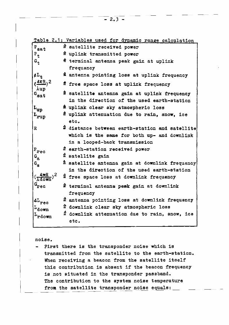
2.1: Variables used for d namic ran e calculation

Prec6=~Ga =

Gs6=

( 4ml )2 4

Adown =Grec A=

~Lrec~=

LdownGo

4Lrdown

~Lt

(4~R)2

AUPGsat

R

~ satellite received power~ uplink transmitted powert terminal antenna peak gain at uplink

frequencyi antenna pointing loss at uplink frequency

~ free space loss at uplink frequency

~ satellite antenna gain at uplink frequencyin the direction ot the used earth-station

• uplink clear sky atmospheric loss~ uplink attenuation due to rain, snow, ice

etc.~ distance between earth-station and satellite

which is the same tor both up- and downlinkin a looped-back transmissionearth-station received powersatellite gainsatellite antenna gain at downlink frequencyin the direction of the used earth-stationfree space loss at downlink frequency

terminal antenna peak gain at downlinkfrequencyantenna pointing loss at downlink frequencydownlink clear sky atmospheric lossdownlink attenuation due to rain, snow, iceetc.

noise.First there is the transponder noise which istransmitted from the satellite to the earth-station.When receiving a beacon from the satellite itselfthis contribution is absent if the beacon frequencyis not situated in the transponder passband.The contribution to the system noise temperaturefrom the satellite transponder noise equals:

- 2.4 -

T"transponder

1 (2-3)

where the used variables are explained in table 2.2.

Table 2.2: Variables used for noise tem~erature calculation1:1Ttransponder : contibution ~o the system noise temperature

from the satellite transponder refered tothe earth-station receiver

~ satellite receiver noise temperature referedto the satellite receiver

~ noise temperature contribution to the systemnoise temperature, indicated by rain absorption

. 4= 250 K = average atmosphere temperature~ antenna main beam factor = 0.9 for this system~ measured clear sky antenna temperature refered

to the earth-station reeeiver.4.- earth-station receiver noise temperature~ total system noise temperature refered to the

earth-station receiver~ total system noise temperature refered to the

earth-station, when receiving an out oftransponderband beacon

The second contribution is the noise temperaturecontibution indicated by rain absorption:

1Train = (1 - L ) .Tabs • '1ardown

(2-4)

where the used variables are defined in table 2.2.

Defining the third contribution Tant and Trec (seetable 2.2), as the total sytem noise temperature

- 2.5 -

refered to the earth-station receiver, Ttot ' can bewritten as:

(2-5)

With a beacon signal which is not within the transponderpassband this is defined as:

(2-6)

For convenience the following definitions are adopted:

(2-7)

(2-8)

The SiN ratio of a received looped-back signal becomes:

S (1 Precw = =~ k.Trec~~

(2~)

where:k = -198.6 dBm/Hz/K (Boltzmann's constant)~ = equivalent noise bandwidth

As an example the dynamic range of the measurement system

- 2.6 -

for a reoeived CW carrier looped through the INTELSAT V.satellite transponder (East spot beam 11/14 GHz) fromthe EUT [2], [3] will be calculated. The followinglink.budget is based on the nominal values in table2.3 [2].

a e • . om na u .~e va ues.constant value

Pt34.8 dBm

G·t60.2: dB

.oLt0.6. dB

(~~K)2 -207.7 dB

Gsat 36.7 dBLup 0.4 dEGa 107.1 dB

Gs 36.2 dB

C'down)2 -2.05.9 dB4itRLdown 0.3 dB

~eo 58.0 dBALreo 0.6 dB

Teat 2200 K

Tant + Trec 301 K

T bl 2 3 Nil link b d t 1

Cup and Cdown defined in equations (2-7) and (2-8) beoome:

Cup = 60.2 dB - 0.6 dB - 0.4 dB - 207.7 dB + 36.7 dB =

-111.8 dB (2-10)

Cdown = 36.2 dB - 205.9 dB - 0.3 dB + 58.0 dB - 0.6 dB =

-112.6 dB (2-11)

It is now assumed that there is the following looped-backrelationship between the up- and downlink fading levels [4]:

(Lrup)in dB's

(Lrdown)in dB's

- 2.7 -

= 1.5 (2-12)

By taking ~ equal to 1 Hz, it is possible to calculatethe SIN ratio per HZ bandwidth also known as thecarrier-to-noise-density ratio C/~. The SIN ratio caneasily be derived from the C/~ ratio by substracting thenoise bandwidth, in Hz, in dB's. The so calculated carrierpower and noise levels of the looped~back measurement atdifferent fading levels is set out in figure 2.2. Porthis specific example, also the cross-polarizationdiscrimin~tion (XPD) (defined below) within the rangeof 0 to 30 dB and its behaviour at different fadinglevels. For this purpose a 10 dE more powerful CW carriera~ a slightly different frequency and orthogonallypolarized to the co-polar signal, would have beentransmitted (see figure 2.3). From this signal only thecross-polar field component is received by the satellite(see figure 2.3). The uplink cross-polar behaviour isshown in figure 2.2 as a dotted area. In the above thefollowing definition is used:

XPD is defined as the square of the co-polar, c~~i,to cross-polar, x~~i, field components ratio of oneand the same signal (see also tigure 2.4):

C(1)(XPD)in dB's ~ 20 log~ (2-13)

Xpol

Cross-polar isolation (XPI) is defined as the squareof the co-polar field component of one signal, c~~i,to cross-polar field component of another signal,X(2 l), ratio, where both co-polar field componentspoare perpendicular to each other (see also figure 2.4):

- 2.8 -

'.~ ..

.."'. .Copolar loop-back signal............ . /

....., .. .. /M=. Xpolar loop-back signal

............ r........ ~. ..........~.. / " . '-

.~ '~

". ......... ..~ ............ .. ...., ... ........... ........ .

......... ... ......... '.;- .-.....::. ".

~ r-.......V '. ..........~./' ".

;/ ~ ..........Min. Xpolar loop-back signal

. 1\-13 .5 dlll )

3D.. 2..

'.

'" ~~38.9

- ceiver noise

.Total noise18.9

system

l- I ,r--- 17

(-173.8)

L--;" -- (-175.1)

/ I\. r---t---.I

""~,----

Sat. Transp. noise I--.(-190.7)

I't~in absorption induced noise

-71

-75;I

1:-ii

-111-lfj

-111

-us-121

-1Zi

-131

-11i

-141

-145

-fi

-CD-Iii

-165

;T -1714.8L, -175

10 log kT -111

noise -1115

dens i ty -Ill

(dBm/Hz) -195-211

-2llS

powerC(dBm)

receivedcarrier

...

attenuation (dB) L + L drup r ow

Fig. 2.2: Dynamic range behaviour of looped-back receivingsystem as a function of up- plus downlink fading

Figure 1: Syste. Block Diagram for theuplInk and downlink (14/11 GHz)depolarization correlation experIment.

Note: cancellation networks are notshown in this fIgure, nor anypreprocessing to give attenuationor XPD levels directly.

I\)

•\D

(1)

(2)

and (4)H

(4)

-- ·_---,

Chart recordereight channels)

minimum)

(5) downlink (5)

fe~eAee Ge pe+- (3)

(4) Uplink X-pol

(3) H

~(4)"// (5) V

~

IRain gauge

/(1)V~(2)H

Rx

Demodulator

------~ Dual-channelTrack In9 Rx

v (1)

V

H (2)

116Hz

Earth Stat Ionup-l Ink

transml tter/51

Earth Stationdown-link lNA(s)and Inter-facll Ityequipment

146Hz

v = vertical polarized eignal

H = horizontal polarized signal

Fig·2.): System block diagram proposed by INI'ELSAT (Ref .22) .

(XPI)in dB's ~ 20

- 2.10 -

C(1)pol

(2-14)

XPI XPD /'

X(2),/

X(1)pol 1/ ,/ pol

• C(2),/ pol

Fig. 2.4: Definitions of XPD and XPI

From (2-9), (2-10), (2-11) and table 2.3 one gets:

Prec = received carrier power (clear sky)­Tant + Trec 301 K ~

Boltzmann's constantcarrier-to-noise-density ratio (clearsky, without phase noise)

-82.5 dBm24.8 dBK

~198.6 dBm/Hz/K91.3 dB/Hz

(+ J(- )

(- )

The clear sky transponder noise temperature refered tothe earth-station can be calculated from (2-3), (2-8)and (2-11):

Ttransponder (clear sky) noise temperature: 620 K

So the degradation in system noise during clear skyconditions due to tr.ansponder noise (see also figure 2.2)becomes:

Ttransponder + (Tant + ~ec)degradation: =(Tant + Trec )

- 2.11 -

620 + 301 = A301 3.05 = 4.8 dB

Using a PLL bandwidthfor 2.4 dB (see figureduring heavy rain, theloss-of-lock condition

1\of 50 Hz = 17 dBHz and allowing2.2) increase of receiver noisedynamic range, defined to a PLLof 10 dB [2], [5], is approximately:

dynamic range =91.3 dB/Hz - 2.4 dB. -17.0 dBHz - 10.0 dB =

61.9 dB

For the beacon transmitter of figure 2.1 one can write,in the case of the INTELSAT V satellite, that itsequivalent isotropically radiated power (EIRP), (P.G)b'equals 37.0 dBm [2J. In the same way as in section 2.1.1.,the beacon power received by the earth-station, Prec,b'is determined:

(2-15)

Por convenience define:

(2-16)

Together with equation (2-6) the signal-to-noise ratiofor the received beacon signal, (S/N)b' becomes:

(3) ~ Prec,b =E' b kTtot bEN,

k (1 -(2-17)

- 2.12 -

Similar to figure 2.2 the beacon-power-to-noise-densityratio as function of downlink attenuation can now becalculated. This is plotted in figure 2.5. The linkbudget is with (2-17) and table 2.3:

beacon EIRPfree space lossatmospheric lossantenna pointing and polarization lossterminal antenna peak gainreceiver noise temperature 316 K t.

(for ~nis receiver)Boltzmann's constantcarrier-to-noise-density ratio (clear sky)

37.0 dBm (-+

205.9 dB (-0.3 .dB (-0.6 dB (-

58.0 dB (+

25.0 dB (-

-198.6 dB/HZ/K (­61.8 dB/Hz

Using a PLL bandwidth of 50 HZ ~ 17 dBHZ and allowingagain for 2.4 dB increase of receiver noise during heavyrain, the dynamic range, defined to a minimum PLLS/N ratio of 10 dB to prevent a frequently occurringout-of-lock condition [2J, [5J:

dynamic range: 61.8 dB/HZ - 2.4 dB - 17.0 dBHZ - 10.0 dB =

32.4 dB

If again the XPD ranges from 0 to 30 dR, tben its valuesare in the dotted area of figure 2.5.

Note that in this case there is no satellite transpondernoise contribution as the frequency of the beacon signalis not within the transponder passband.

It is evident that the co-polar signal which is transmittedback from the satelli~e to the earth-station also has adownlink cross-polar component. Because the satellitetransponder noise only contributes significantly to the

- 2.13 -

-

I 1 1:---

T

5 '-/Copolar beacon level

f-- r--...tV

.--.......I--- '--

I--..r--~

(-131.8)

'" . . •.. 30 idB. .."

.-.. ... ....

Minimum Xpolar level beacon. ....

. ... -161 • )

9·t171.4

. T-173.8

~ \Tlal system

-175.1

/ ~. noise

"system noise clear sky (1'ant 1'ree)

f+

'-t.bsor:ption induced noise

11:( 1 - l/Lrdown) Tab" r a

Tabs·250K

r20.9~ antenne maina

beam factor

.... - c=

-111

-11

-121

-1Zi

-~

-las-1G

-US

-191

-155

-11i1

-lffj

-171

-175

-111I

-185

-1!11

-195

-2lIl

-2l!i

10 log kT

noisedensity(dBm/Hz )

powerC

(dBm)

receivedcarrier -lBS

attenuation (dB) Lrdown

Fig. 2.5: Dynamic range behaviour of beacon receivingsystem as a function of downlink fading

- 2.14 -

total system noise at low attenuation levels and XPDis then considered large [6]; ita contribution isneglected in this situation. The link downlink XPDbudget 1s plotted in figure 2.6.

In the above calculations no account was taken of thephase noise spectral densities of signal sources andlocal oscillators in the transponder, the transmitterand the ground station.

2.2. Calculation of rms phase jitter with arbitraryphase noise spectrum

The inherent phase noise of up- and down-convertors andsatellite local oscillators can become a significantfactor in the design of carrier tracking loops forpropagation measurements and for coherent digitaldemodulation. To study its effects a characterizationof oscillator phase noise which can be related tomeasurable parameters is used.

In a situation like that of paragraph 2.1 (see figure 2.1)the following assumption is made (see figure 2.7):

there are three oscillators which contribute to thefinal phase jitter, namely:

a) the transmitter oscillatorb) the satellite translator oscillatorc) the local oscillator in the receiver

The spectrum which is transmitted back to the earth-stationis attenuated and proportional with (1/Lrup ). In thesatellite this signal is mixed with the signal from thesatellite oscillator. So the spectrum which is transmittedback to the earth is the convolution of both spectra.

- 2.15 -

received

looped- 71t----r-----r---,---r----r---r--.--.,.----,---+

baek C0- ) ~,+---t---t--+----I--+--+---!--..J--I---I

and cross- ..polarpower(dBm)

'".~ _,--162.

-+--4-----1 a. <;

Receiver noise

Noise due to rain absorption

-9 t----i--+--t---+--+----...1,.--+~,:...+.~....j....:...-:...j

-1S5t----r---t--t--f--f---f-----lI--+::-;.--t-=--:....j-'. . .-lfAl+--l----I~-l--165 _~ Total system noise

-171~~§~~~~~~~~...L--1~t== -171.4

-111 l.--"'\-lei / I\.

I-iraoII----+---+--

-l!ir.---t--t---t--+----+--+--+--+---l----l-Zl t----i--+--t---t--+----...1---+--l---I----J

-2I5_f---::.,.,:t---=:t---;::1--=:1-----:-::I--:I--+--+--+---------+~ ~ ~ ~ ~ ~ ~ Q ~

~

10 log kTnoisedensity(dBm/Hz)

attenuation (dB) Lrup + Lrdown

Fig. 2.6: Dynamic range of downlink XPD as a functionof up- plus downlink fading

- 2..16 -

This signal is again attenuated and proportina1 to (1/~down).

As before this signal is mixed, now with the localoscillator output. For the received spectrum, which isthe convolution of both spectra one can then write:

s (w) = L 1 .K2 .[ fL 1 .K1 .S (OJ)} ~ s (w) ] ~ S (w) (2-18);,rec rdown rup ;,up ¢,sat p,LO

where the variables used are defined in table 2.4.Hence:

S (w) ::: Kls (w) ~ S (w) ~ s (w)l.t 1 .t 1I,rec I I,up ;,sat ;,LO rup rdown

Furthermore one can write (see paragraph 2.1.):

(2-19)

(2-20)

where the used variables are defined in table 2.4.

From (2-18) the phase noise spectrum from the receivedsignal is determined. It is clear that it is proportiQna1with 1/(Lrup.Lrdown). However its shape stayes the same.Therefore the phase noise spectrum of the round-tripearth-station, satellite signal can be written as:

1 1S (w) ::: S (w) •......-.'!!!""L-.;,.-o,rec 0 ~rup rdown

(2-2.1)

where:S (w) ~ the received phase noise spectrum when botho

up- and downlink attenuation equal unity

- 2.'7 -

atmosphere

ransmitter

1s, satr-------.translator

satellite

/atmosphere

Lrdown

I~o

Table

K,K2S' (w);,up

S (w)~,sat

S (uJ)15.LO

S (w)_,rec

Co

Fig. 2.7: Typical system set-up with noise spectra oftransmitter, translator and local oscillator

2.4: Variables used for phase noise spectrum calculation~ constant~ constant~ transmitted spectrum (no data modulation)

A spectrum of satellite translator oscillator

A spectrum of local oscillator in receiver

4 received spectrum

~ received carrier power when both up- anddownlink attenuation equal unity

= N (L ,L d ) ~ total system thermal noise densityo rup r ownwhich is a function of Lrup and Lrdown

- 2.18 -

Note from (2-18) that phase-noise from several sources.cannot simply be added. It therefore differs fromadditive noise and is called multiplicative noise.

In general, the output of an oscillator can be modelledin the form:

(2-23)

where ,s<.t) is the phase noise given Wc and thereforejCt) : O. The single side phase noise spectrum is assumedto be described by the followdng form [7]:

01 02 O~S (w) =)" + ~ + ~ + 04

; w w w

where:S (c.u), 4 phase noise power spectrum

and where 01 through 04 are suitably chosen positiveconstants. To calculate the total amoun~ of phase jitter,criT' the mean square phase noise for a "small" amountof phase jitter in a phase-Iocked-Ioop may be related tothe root mean square (rms) frequency deviation as follows

[8]:w2

<!'~(ClJ1'W2) = J S (w).11 - H(UJ) I2dw (2-24)

w1 ~

where:"01 - W

2~ equivalent angular noise bandwidth of

measurementcr~(w1'W2) ~ the mean square phase noise within this rangeBXw) ~ the phase-locked-loop linearized transfer function

For a high-gain second-order loop [8], with damping factor:

- 2.19 -

~ d = 0.7071

H(w) becomes:

1 + jW:n~w) = ~ -

1 + jw'tp - (w 'p2)/2

where:T .. 3

p. ~

in which:£L ~ equivalent loop noise bandwidth

In this situation:

(2-26 )

(2-28)

A damping factor of 0.7071 has been chosen because i~

simplifies the resultant integrals in equation (2-28)and because it is a commonly adopted value. Results forother damping factors may be found in a similar manner.In [7] only the first two integrals of (2-28), whichnormally dominate at low frequencies, are retained.Here all four terms of (2-28) are calculated. To do soan additional assumption has to be made, namely that thelast two components of (2-23) are bandlimited becauseboth corresponding integrals of equation (2-28) do notconverge. This is no real limitation, because the actualphase noise power spectrum is normally bandlimited for

- 2.20 -

systems,due to bandpass filtering at the intermediatefrequency (IF) level.

To express this bandlimitation define:,

o ~ tV ~ 2~.BIF[CJ for

C3 = 0 for w > 27t.BIF,

S. w S 211.[C4 for 0 Be

C4 = 04

for w ~ 2Jr. BC4

(2-29)

(2-)0)

where BIP is the equivalent bandwidth of the IP filterand BC the bandlimitation of C4 (see figure 2.8). In

4 t rthe rest of this chapter the accents in C) and C4 areleft out for convenience.

10 log IS;("')11

30 dB/decade

dB/decade

10 dB/decade

.....·7 .- .- .-'. ~. -thermal noise

10 logw

Fig. 2.8~ Example of phase noise spectrum

- 2.21 -

The first integral of (2-28) is calculated bysubstituting z • w2 , the second and fourth with helpof complex function theory and the third by substitutingz = ~4e Since all integrals converge (with (2-29) and(2-30) that is), the upper limit is taken as ~ and thelower as 0, yielding an upper bound on cr:. Iiere onlythe results of these calculations, which can be foundin Appendix A, are given. To calculate the contributiondue to the oscillator phase noise, three differentsituations, are looked upon. The first two will lead tothe same results. These situations apply only to thelast integral in (2-28). The other three remain the samenamely:

9C1 X"1 1 = -----

128~

3C27\"

~=­16Br,

C3 { , 4 4}I 3 = Te In 11 + T· (271". Btl?)

where:11 ~ first integral of (2-28)12 ~ second integral of (2-28)1

3~ third integral of (2-28)

When:

(2-31)

(2-32 )

(2-33)

1296Jt4.B 4= r- »1 (2-34)

1024.Br,

which is normally valid, 13

can be approximated by:

- 2.22 -

(2-35)

Consider three situations for the last integral of (2-28):

c) Br, > BC4

(2-j6 a)

(2-36 b)

(2-36 c)

a) It can be shown that (Appendix A), if (2-36 a) isvalid the fourth integral of (2-28) equals:

for R.. « B-LC4

(2-37)

where:14 ~ fourth integral of (2-28)

b) If (2-36 b) is valid, 14 equals (Appendix A):

27\'.C4.~14 = C4 .27f.BC4

- 3 .F (with F ~ 1)

for 1\ ~ Be (2-38)4

where:

F = F(!1) (2-39)

- 2..23 -

It can be shown that in this situation:

0.99 < F ~ 1 (2-40)

c) If (2-36 c) is valid one obtains (Appendix A):

2"'.C4·BLI 4 := C4.2Jr.BC - j .F for ~ > BC (2-41)

4 4

where:

F = F(~) =

in which:

dz =

3]1' .02'12

Jo

2'12'-7r dz

z4 + 1

(2-42)

B4 C4

c = c(~) = BL and 0 < c(~) < 1 (2-43)

(2-44)

Finally the phase jitter contribution due to phase noisecan be calculated from (2-28),(2.-31),(2-32),(2-35),(2-37),(2-38) and (2-41):

<T~ = 9C 1~ + 3C2X + C3

.ln!37t. B1F I - c3·lnl B1 I +

F 128B£ 16B1 2V2 (1HZ) (1Hz)

21t.C4. B1C4

.2:1'\BC - j .F4

where:

o < F < 0.992 otherwise

F ::: 1 for Br. ~ Be4 (2-45)

The actual values of Ftable 2.8 in paragraphF will be equal ~o 1.

- 2.24 -

for different c can be found in2.3. Usually ~ «BC so then

4

(2-46)

l' =

Cr=o

The thermal noise contribution to the phase jitter isgiven by [7]:

2 ~(j~ th = J'M(C/No)

where:correction factor to account for the loss in SINratio due to frequency doubling or remodulationin the carrier recovery loop [9]

M = correction factor to account for SiN degradationin the receive filter [10]carrier-to-noise-density ratio at the down­covertor output

Therefore, summing (in a mean square sense) the totalphase jitter yields:

2 9C17( 3C2X 11\ IuJm = 2 + - C3·1n +p~ 128BL 16BL (1Hz)

[VJ[(C1/NoJ - 211";C

4•1-]' Br, + C3.Inl }k· (:::J

(2-47)

2.3. optimum PLL bandwidth

In paragraph 2.2 the total phase jitter is calculated,(2-47). It is clear from (2-28) that the total phasejitter is a function of the loop bandwidth ~ in thereceiving system. The errors caused by phase jitter in

- 2.25 -

carrier tracking loops, for e.g. propagation measurementsto measure depolarization and attenuation or for coherentdigital demodulation, are now minimized.

First a condition, that must be satisfied to minimizeerrors in a coherent digital demodulation system, isderived. Later it is shown that, this condition staysthe same for the propagation measurement systems.

It has been found empirically that the mean time tounlock for a second-order-phase-locked-loop, Tav ' isapproximated by the formula [7] (see figure 2.9):

(2-48)

where:Wn ~ the loop natural angular frequency

(f->L ~ the signal-to-noise ratio in the loop noisebandwidth

Using the high SiN ratio approximation [7] for (S/N)L:

( S) .., 1!f L - 2

2~L

where:~~ ~ the root mean square phase jitter

With (2-25),(2-48) and (2-49) one gets:

If ':! 1:..Q§.. expI 7t' IaV ~ ~

~

(2-49)

(2-50)

Some experimental results have shown [7] that the meantime during which the loop remains unlocked, TUL , may

- 2.26 -

be approximated by (see figure 2.9)~

(2-51 )

time to unrock with average: 'rav

~ H ~ ~ H H.in lock+---"'"

out-of-Iock - - -~---I- - -

time during which loop remains unlocked with average: TUL

Fig. 2.9: Time intervals during which the PLL is in andout-of-Iock

Using (2-50) and (2-51) and assuming an error rate of0.5 during an out-of-Iock condition yields the followingaverage probability of error contributed by cycle skipping(which occurs when the dynamic phase-error magnitude ofthe PLL exceeds 21T [10]):

where the used variables are defined in table 2.5.

When a Costas loop is used, the effective phase jitterwhich contributes to cycle skipping is [7], [9]:

(QPSK) (2-53)

- 2.27 -

Table 2.5: Variables used for probability of errordetermination due to c cle skit bitrate~ probability of error contributed by

cycle skippingt = P [£/csJ ~ error rate during out-of-Iock conditionp rcs--r ~ number of bits durin~ cycle skip = TUL .Rb

~ ~ total number 0 bits Tav.Rb

Renee (2-52) becomes:

7r 1 -it IPees = '4. exp 2320p

(2-54)

To obtain the overall bit-error-rate, (2-54) must becombined with the probability of error due to thermalnoise. In the event of infrequent cycle skipping, errorsdue to thermal noise occur between cycle skips and areindependent thereof. The thermal noise contribution istherefore combined as an independent variable. Por bothbinary phase shift keying (BPSK) and quadrature phaseshift keying (QPSK) one gets:

Peth = Q{J~ob'l (2-55)

where:

Q(O(.)

Pe th = probability of error due to thermal noiseEb = energy per bitNo = noise power density

Hence, the combined probability of error is:

- 2.28 -

Pe = P [E/cs] .P [cs] + P [Elno cS].P [no cs] (2-56)

where :p[S/csJ.p[cs] is given by (2-52), andP [£1no c s] ~ P e th

p[no cs) =[1 -~.exP{2~11] "'1, for all cases

of operational 1nteres~

and where the used variables are defined in table 2.6.

Table 2.6:PeP [E/no cs]P[no cs)

Variables used for oint robabilit of error~ combined probability of transmission errort error rate during lock condition6=

total number of bits - number of bits during cycle skiptotal number of bits

Therefore:

Pe =:! Pecs + Pe th ~ ~. expj -~21 + Q{/~Ebl32<T',r 0

(2-57)

Since a~~ is a function of ~, (2-47), so is PeePe can be minimized by determining the optimum BL•To this end the derivative of (2-57) is determined.

2First substitude z = ~~. Then:

dPe dPe dzcrnr: = az·~

2where, z =~~T and note that:

(2-58)

- 2.29 -

dP e 7't2

I-~Jaz-- = 128z2•exp ~ > 0 (2-59)

Furthermore with (2-41), (see Appendix A) one obtains:

2dz . ~ ~~T _ -18C 1lr _ JC2 7f

dJL - - 1281\J 161\2

(2-60)

where:3K .c

2VZ

Jo

an. z4zr dz

4 2(z + 1)

and

(2-61)

So out of (2-58), (2-60) and (2_-61) one obtains:

(2-62)

Setting the derivative of Pe to zero and checking itssign around the so found zero, it is possible to determinethe ~ for minimum Pee out of (2-59), (2-60) and (2-62)it is clear that this equals:

2

~~? = 0L

Furthermore from (2-58) and (2-59):

(2-63)

- 2.30 -

IdP I {dCT2 j

sign~ = Signl~ (2-64)

In carrier tracking loops for correlation measurements,minimizing errors equals minimizing phase jitter in theloop. So also in this situation the optimum BL isdetermined out of (2-63).

So ~ is determined out or:

Two different situations are considered:

a)

b)

1 +-2KC4 >0J'M(C/No) J

1 -2KC4 (0JlMCe/No) + j

1+

-21fC4 >0vMCC/No) j

(2-66)

(2-61 a)

(2-67 b)

When ~ cannot be estimated, case a) is the starting point.

a) If (2-66) is valid (2-65) equals (see Appendix A):

(2-68)

-2KC4j = 0

which corresponds with: G =1, and where the term betweenbrackets is positive.

- 2.31 -

This can be written as:

(2-69)

where «, (3' 1 and /) are defined in table 2.7.

Table 2.7: Definitions of« and 6.

3Multiply (2-69) by ~ >0:

B 3 _1"FL 2 _1l"FL =~ (2-70)L &-L &-L b

or:ClC.

= -6(2-71)

Estimating the 1eft-hand-side, k(~), of (2-71) gives:

k(~) = ~{BL2 - f~ - r} equals zero for:'

= 0 and for,

= f :!: V(f) 2 + 4 12

(2-72)

In which ~ ,BL and ~ are the roots of the left-hand­123

side of (2-71). Together with table 2.7 one 'obtains:

(2-74 a)

- 2.32 -

(f)2 + 4(f) > 0 and,

.l. _ V( 1.) 2 •+ 4(t)

~_ 6 & < 0 (2-73)

1 2

V(L)2,

L+ + 4C/J )

Br,3= 6 § & >0

2

Furthermore the rigbt-hand-side of (2-71) t> o.Both the left.-hand-side and the right-hand-side of:equation C2-11) are plot.t:ed in figure 2..10. Only ther~ght-half-plane of figure 2.10 is of interest becauseit corresponds with pos1.tive values for the loopbandwidth Et. The loop bandwidth ~ for which the lef~­

hand-side is the optimum Bl . From e~ation (2-71)dcr2 opt

one learns tha~~ is negative for values of EL which

are smaller than ~ and positive for values of ~opt 2

larger than ~ • So 0""'T is minimum for this Br..opt l'

Now check if equation (2-66) is valid, if not continuewiith case b).

b) If equation (Z-67 b) is valid first calculate ~opt

as before, then determine the corresponding G (out of\J-61 )J. and continue with cas e b).. but take G as justfound.Accordingly (2-67 a), (2-67 b) and (2-68) change into:

1 2ifC4vM(O/No) - ---,-.G > 0

(2-74 b)

-2KC4+ j .G = 0

(2-74 c)

- 2.33 -

left-hand-side

+right-hand-side

opt

~ig. 2.10: Optimum loop bandwidth R­~op~

This procedure is continued until the optimum BLis calculated with the desired accuracy. opt

If (2-67 a) is valid, first estimate G by:

1

(2-75)

- 2.34~

This value of G corresponds to a certain Et (table(2.8).

No~ estimate G again by substituting the ~ thisestablished in (equation (2-65.».

(2-76 )

By repeating this last step until ane reaches thedesired accuracy one can determine ~ •

opt-

However in most cases where (2-67 a) or CZ-6l' b) isvalid, the terms of (2-65) which include ~ can beneg~ected, because Br,» 1, so equat,ion (:2-75) isvalid and G can be directly determined 'ou.t:. of it. 'rhecorresponding ~ is the optimum loop bandwidth Ei •

opt

After, determining the optimum loop bandwidth ane candetermine the total phase jitter by substituting~ and its corresponding value of F into (2-47).

opt.

In table 2.8 F and G are calculated for several valuesof c.

By substituting (2- 20) and (2- 21) in (2-46) and(2-24) respectively and in which Lrup and Lrdownare taken constant, one can compute the optim1w loopbandwidth out of (2-65) and with this the phase jitterout of (2-47) for various fading levels.

With respect to [71 the following can be concluded.

- NOD- of the terms of (2-24) has been neglected, so amore accurate calculation of the total phase jitterhas been made ..

- 2.35 -

Table 2.8· F and G versus c •.

37r 3]{2lZ C 2(i.c

2 2Be J SV2. z 4 I 2V2

C :& C(B:r) =~ G • if dz F = -r dz2 z4 + 1o (z4 + 1) 0

L..OO 0.968 0.99"20.9, Q.962. 0.9910.90 0.956 0.9890.85' 0~948 0.98T0.80 0.938 0.9840.15 0.925 0.9810.70 0.908 0.9770.65 0.886 0.9710.60 0.857 0.9630.55 0.819 0.9530.50 0.766 0.9380.45 0.695 0.9180.40 0.599 0.8880.35 0.475 0.8440.30 0.330 0.7800.25 0.186 0.6920.20 0.775 • 10-1 0.5790.15 0.210 • 10-1 0.4450.10 0.292 • 10-2 0.2990.05 0.924 • 10-4 0.150

- 2.36 -

- Furthermore the determination of the ~otal phase ji~ter

is valid for a much wider range of values of Bi. Thisis necessary due to the rather poor phase noiseperformances of the various oscillators in the to beconsidered system, which requires BL to lbe large.

- fhe phase jitter contribution due to phase noise isindependant of up- and downlinkfading levels, because thephase noise spectrum refered to the received carrierpower stayes the same for various fading levels.

- The optimum loop bandwidth is analytically determined.~or relative "clean" carriers (which allow a small loopbandwidth), this calculation becomes rather simple.

-Finally, for both measurement and coherent digitaldemodulation carrier tracking loops, it was shown thatthe optimum loop bandwidth is derived from the same equation.However, it should be noted that, while a carrier ispresent in propagation measurements, it has to berecovered in most digital demodulators, since normallysuppressed carrier modulation is used in satellitesystems.

_ As an example, the degradation due to phase noisefor the system present at EUT, will be calculated in

chapter 4.

- 3.1 -

3. ADAP'llVE COMPENSAnON OR XPD.

By using two orthogonal polarizations simultaneously,one can in principle double the capacity of a radiocommunication system ~1]. However polarization variationwithin the antenna beamwidth will introduce significan~

depolarization. This may happen during rain.Depolarization causes degradation and therfore has to beinvest.igat.ed. Propagation measurementB (paragraph 2.1-)c.cmld provide this information.In practice, the t.wo orthogonal polarizations leaving thetransmit~er are either two orthogonal linearly polarizedwaves or two circularly.polarized waves with opposite senseof rotation (clockwise and counterclockwise). Whateverthe cause of polarization distortion, the failure to .maintain orthogonality will produce two non-orlhogonalelliptically polarized waves at the receiving terminal.In this chapter this is expressed in mathematical termsand furthermore several principles of recovering orthogonalityare shown: In order to determine which principlescan be applied and which is best in terms of optimumcompensation, costs and complexity, information about thecorrelation between co- and cross polar field componentsand the correlation between up- and downlink frequencycross-polar field components is needed. This informationcould be obtained fram propagation measurements [12].

3.1.Theoretical background C11,12,131

Two nonorthogonal elliptically polarized waves, I andn, can be represented by two polarization ellipses withtheir major axes oriented at an arbitrary angle 8 withrespect to each other as shown in figure 3.1. The axialratios (see figure 3.1) At and A2 are of the same oropposite sign depending on whether the polariz:ationvector are rotating in the same direction or not.The two elliptically polarized waves are represented in

- 2.26 -

be approximated by (see figure 2.9)~

(2-51 )

time to unrock with average: 'rav

~ H ~ ~ H H.in lock+---"'"

out-of-Iock - - -~---I- - -

time during which loop remains unlocked with average: TUL

Fig. 2.9: Time intervals during which the PLL is in andout-of-Iock

Using (2-50) and (2-51) and assuming an error rate of0.5 during an out-of-Iock condition yields the followingaverage probability of error contributed by cycle skipping(which occurs when the dynamic phase-error magnitude ofthe PLL exceeds 21T [10]):

where the used variables are defined in table 2.5.

When a Costas loop is used, the effective phase jitterwhich contributes to cycle skipping is [7], [9]:

(QPSK) (2-53)

- 2.28 -

Pe = P [E/cs] .P [cs] + P [Elno cS].P [no cs] (2-56)

where :p[S/csJ.p[cs] is given by (2-52), andP [£1no c s] ~ P e th

p[no cs) =[1 -~.exP{2~11] "'1, for all cases

of operational 1nteres~

and where the used variables are defined in table 2.6.

Table 2.6:PeP [E/no cs]P[no cs)

Variables used for oint robabilit of error~ combined probability of transmission errort error rate during lock condition6=

total number of bits - number of bits during cycle skiptotal number of bits

Therefore:

Pe =:! Pecs + Pe th ~ ~. expj -~21 + Q{/~Ebl32<T',r 0

(2-57)

Since a~~ is a function of ~, (2-47), so is PeePe can be minimized by determining the optimum BL•To this end the derivative of (2-57) is determined.

2First substitude z = ~~. Then:

dPe dPe dzcrnr: = az·~

2where, z =~~T and note that:

(2-58)

- 2.30 -

IdP I {dCT2 j

sign~ = Signl~ (2-64)

In carrier tracking loops for correlation measurements,minimizing errors equals minimizing phase jitter in theloop. So also in this situation the optimum BL isdetermined out of (2-63).

So ~ is determined out or:

Two different situations are considered:

a)

b)

1 +-2KC4 >0J'M(C/No) J

1 -2KC4 (0JlMCe/No) + j

1+

-21fC4 >0vMCC/No) j

(2-66)

(2-61 a)

(2-67 b)

When ~ cannot be estimated, case a) is the starting point.

a) If (2-66) is valid (2-65) equals (see Appendix A):

(2-68)

-2KC4j = 0

which corresponds with: G =1, and where the term betweenbrackets is positive.

(2-74 a)

- 2.32 -

(f)2 + 4(f) > 0 and,

.l. _ V( 1.) 2 •+ 4(t)

~_ 6 & < 0 (2-73)

1 2

V(L)2,

L+ + 4C/J )

Br,3= 6 § & >0

2

Furthermore the rigbt-hand-side of (2-71) t> o.Both the left.-hand-side and the right-hand-side of:equation C2-11) are plot.t:ed in figure 2..10. Only ther~ght-half-plane of figure 2.10 is of interest becauseit corresponds with pos1.tive values for the loopbandwidth Et. The loop bandwidth ~ for which the lef~­

hand-side is the optimum Bl . From e~ation (2-71)dcr2 opt

one learns tha~~ is negative for values of EL which

are smaller than ~ and positive for values of ~opt 2

larger than ~ • So 0""'T is minimum for this Br..opt l'

Now check if equation (2-66) is valid, if not continuewiith case b).

b) If equation (Z-67 b) is valid first calculate ~opt

as before, then determine the corresponding G (out of\J-61 )J. and continue with cas e b).. but take G as justfound.Accordingly (2-67 a), (2-67 b) and (2-68) change into:

1 2ifC4vM(O/No) - ---,-.G > 0

(2-74 b)

-2KC4+ j .G = 0

(2-74 c)

- 2.34~

This value of G corresponds to a certain Et (table(2.8).

No~ estimate G again by substituting the ~ thisestablished in (equation (2-65.».

(2-76 )

By repeating this last step until ane reaches thedesired accuracy one can determine ~ •

opt-

However in most cases where (2-67 a) or CZ-6l' b) isvalid, the terms of (2-65) which include ~ can beneg~ected, because Br,» 1, so equat,ion (:2-75) isvalid and G can be directly determined 'ou.t:. of it. 'rhecorresponding ~ is the optimum loop bandwidth Ei •

opt

After, determining the optimum loop bandwidth ane candetermine the total phase jitter by substituting~ and its corresponding value of F into (2-47).

opt.

In table 2.8 F and G are calculated for several valuesof c.

By substituting (2- 20) and (2- 21) in (2-46) and(2-24) respectively and in which Lrup and Lrdownare taken constant, one can compute the optim1w loopbandwidth out of (2-65) and with this the phase jitterout of (2-47) for various fading levels.

With respect to [71 the following can be concluded.

- NOD- of the terms of (2-24) has been neglected, so amore accurate calculation of the total phase jitterhas been made ..

- 2.36 -

- Furthermore the determination of the ~otal phase ji~ter

is valid for a much wider range of values of Bi. Thisis necessary due to the rather poor phase noiseperformances of the various oscillators in the to beconsidered system, which requires BL to lbe large.

- fhe phase jitter contribution due to phase noise isindependant of up- and downlinkfading levels, because thephase noise spectrum refered to the received carrierpower stayes the same for various fading levels.

- The optimum loop bandwidth is analytically determined.~or relative "clean" carriers (which allow a small loopbandwidth), this calculation becomes rather simple.

-Finally, for both measurement and coherent digitaldemodulation carrier tracking loops, it was shown thatthe optimum loop bandwidth is derived from the same equation.However, it should be noted that, while a carrier ispresent in propagation measurements, it has to berecovered in most digital demodulators, since normallysuppressed carrier modulation is used in satellitesystems.

_ As an example, the degradation due to phase noisefor the system present at EUT, will be calculated in

chapter 4.

- 3.2 -

X-Y coordinates where their major axiSat an counterclockwise angle of rotationrespectively from the X-axis. (P2 in theof figure 3.1, is a negative value).

X1 and X2 areof /31 and,t12 .configuration

POLARIZATION eLLiPse I

AXIAL RATIO IA,I = g~x,

POLARIZATION eLLiPse n

AXIAL RATIO IAzl =g~

fig. ).t: Two nonorthogonal elliptically pOlarized waves[11] •

The rati.o of clockwise to counterclockwise circularlypolarized field components for the polarization ellipseI, Q1' will now be derived.For the electrical field vector of the polarization ellipseI, E1, one can write (see figure 3.1), [13]:

j I j wt - j (~ + ~1) -lOCS .e .8y

where:

for Iclockwiseelliptical (3-1

counterclockwiseelliptical

Aex unity vector in X-direction

ey ~ unity vector in Y-direction

- 3.2 -

X-Y coordinates where their major axiSat an counterclockwise angle of rotationrespectively from the X-axis. (P2 in theof figure 3.1, is a negative value).

X1 and X2 areof /31 and,t12 .configuration

POLARIZATION eLLiPse I

AXIAL RATIO IA,I = g~x,

POLARIZATION eLLiPse n

AXIAL RATIO IAzl =g~

fig. ).t: Two nonorthogonal elliptically pOlarized waves[11] •

The rati.o of clockwise to counterclockwise circularlypolarized field components for the polarization ellipseI, Q1' will now be derived.For the electrical field vector of the polarization ellipseI, E1, one can write (see figure 3.1), [13]:

j I j wt - j (~ + ~1) -lOCS .e .8y

where:

for Iclockwiseelliptical (3-1

counterclockwiseelliptical

Aex unity vector in X-direction

ey ~ unity vector in Y-direction

- 3.3 -

The corresponding clockwise (Ec ) and counterclockwise eEcc)circularly polarized field components are [13]; .

jwt - jp1- jwt~ = i(OD + OC)e e..... + iCOD .± Oc)ec - ~

+ j ~ . jwt - j C~ - t9 )'-1e _ '(OD + OC)e ~ (1 ex ~. 1

{

clockwise ellip~cal

C).-Z)counterclockwise elliptical

and:

for

(3-3)

wbere A1 is positive for clockwise rotating ellipticalpolarization and negative for counterclockwise rotatingelliptical polarization.

The electrical field vector can also be written as:

{i-(ODjwt - j(3 jwt + j(31!-+ OC)e 1 + ';COD + OC)e ex +

Ii-CODj<.IJt - j(~ + f1) _ jOlt - j (! - (31 1/-+OC)e iCOD - OC)e ey =

(3-4)

where:

~ t(OD +jwt - j(l1 jwt + jP1

Ex OC)e + ';(OD - OC)e

~jo>t - j (~ - (31 ) jwt - j C~ - (31 )

Ey ';(OD + OC)e - !(OD - OC)e

- 3.4 -

The ratio (P1 ) of the Y component Ey to

Ex for the polarization ellipse I is:1r

- q1 -j(~)

+ q1· e

X component

( 3-5)

Substituting ()-3) into (3-5), an expression for P,is determined. Similair Pz is found for the polarization

ellipse n.It is found tha~:

(1+Ai2

) - (1-Ai2).cos 2~i l [ 2Ai

2 2 .exp j arctan -.--""2-~--(1+Ai ) + (1-Ai ).cos 2(3i (1-Ai ).sin 2(Jj

i = 1,2 (3-6)

In order to convert an elliptic polarization into a

1inear_ polarization, the phase difference between the X

and Y field components must be eli~inated by a suitable

differential phase shifter. Considering two elliptic

polarizations, the condition for simultaneous

transformations into two linear polarization is [11J:

or (3-7)

The above equations are equivalent to:

()-8)

substituting (3-6) into (3-8), and using the relation

~2. = (31 - a, the solution for (31 is [13]:

/31 = ~arctanlcos 29

- 3.5 -

sin 29(3-9)

The above expression fixes the orientation of the X - y

coordinates. By applying a suitable chosen phase shift

arg P1 to the components in the Y direction, the two

ell~ptically polarized waves are transformed into two

linearly polarized waves. For this phase shift one can

n.ow write:

2.A.14. fJ = arctan

in which~

The angle bet~een the two linear polarization vectors

is:

t= {arg P1 + K = arg P2

forarg P1 = arg P2

(3-11 )

and where Ip11 and jp21 are given by equations (3-6)0

tis not recessarily a right angle. However, this angle

can be changed to a right angle in the following manner.

- 3.6 -

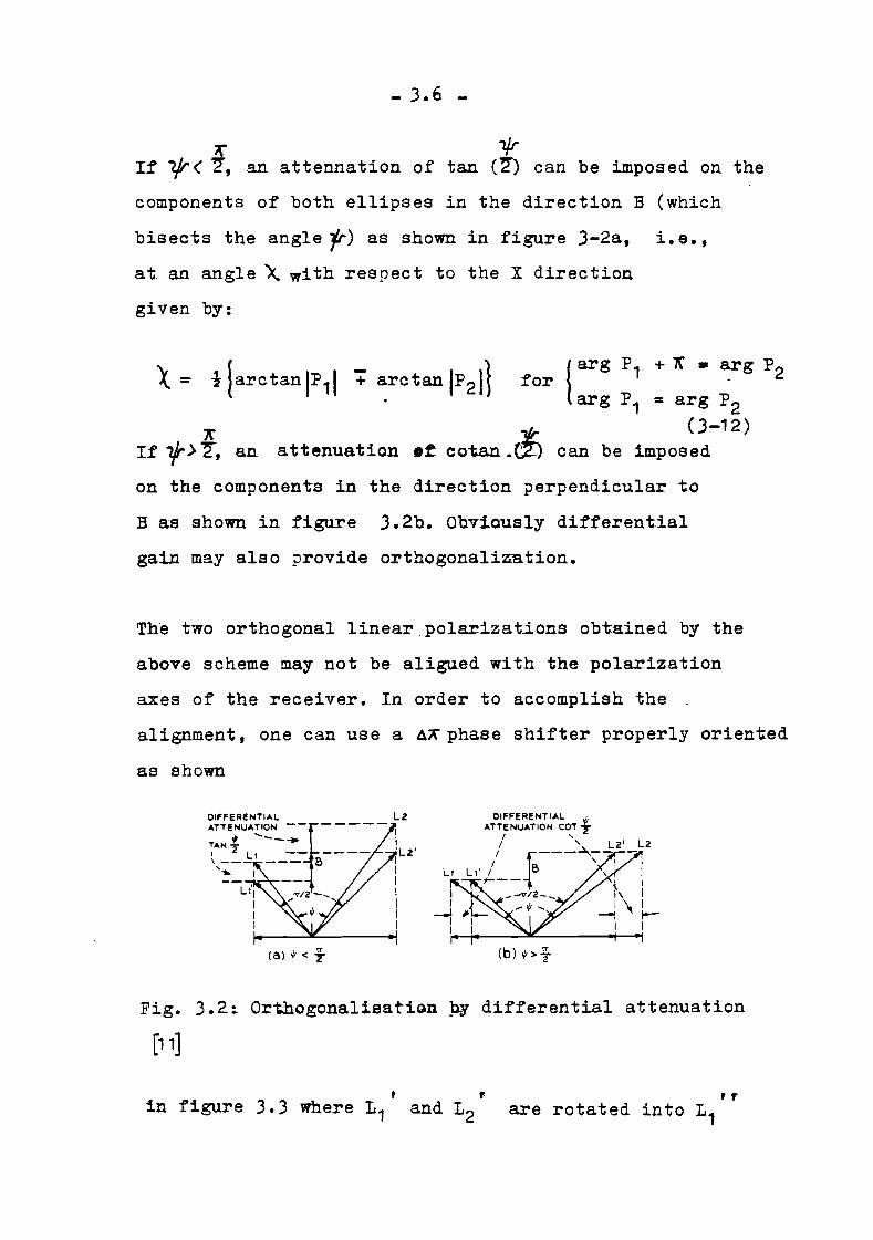
it" 1jrIf" 1j/'<~, an attennation of tan (~) can be imposed on the

components of both ellipses in the direction B (which

bisects the angle y) as shown in figure 3-2a, i.e.,

at. an angle X with respect to the X direction

given by:

7\If 1(>~, an

larg P1 + 7( • arg P2for .arg P1 = arg P2

(3-12)attenuation .:t cot.an Ai!:> can be imposed

on the componen~s in the direction perpendicular to

B as shown in figure 3.2b. Obv:Lously differential

gain may also provide orthogonalization.

The two orthogonal linear.polaxizations obtained by the

above scheme may not be ali~ed with the polarization

axes of the receiver. In order to accomplish the .

alignment, one can use a AAphase shifter properly oriented

as shown

(a) '" < t (b) Ii> t

Fig. 3.2~ Orthogonalisat~Gn~y differential attenuation

in figure 3.3 where L1f r

are rotated into L1

- 3.7 -

,,and L2 • This ~~ phase shifter can also be plaeed

in front of (or immediately after) the ~arg P1 phase shifter.

Then the orientations of the differential phase shifters

and the differential attennator must be changed accordingly.

,;r--o::;t::::-r---2=::::._L 2.'t.",PHASE SHIFTER---'

Rig. 3.3: Rotation by. A'f section [11]

The depolarizing effec~ of rainfall have been, and st2ll

are, subj ect t·o investigation both analytically and

experimentally (see review in [12]). Figure 3.4 shows

cross-polarization isolation (XPI) at 4,6 and 11 GBz

versus rain rate over a assumed 5 - km path length in a

sa~ellite link from COMSAT Labs Clarksburg Maryland U.S.A.

to the INTELSA~ V satellite. The incident waves are assumed

to be perfectly circularly polarized. These data, obtained

from [14] represents the worst-case degradation of the

polarization state due to rain. It is important to note

that the effect of differential phase shift is the major

source of isolation degradation at frequencies up to about

10 GHz. Where the effect of differential attenuation can be

neglected (figure 3.4 and [12}), adequate cross~polarization

isolation (XPI) can be achieved at certain rain rates

- 3.8 -

with differential phase correction only.

,,0 ~---r----"'-----'----'----'------r----,

'5l~ GH:

35

--- EFFECT OF DIFFERENTIALPHASE

II GHz

4 GHl \

\G GHl \ \\

\ '\

\ "\ "11 GHl \

\ '\\ '\

\ "\ "

'\ "'\ "'\ ......" ......" ...... ," ," "" ...." ........

.......... .... .........-- EFFECT OF OIFFERENTIAL " .............

ATTENUATION " , ....................................

10

15

z'" 30<:(5~

Z

§ 25

<".~:s2 20

25 50 75 100 125 150

RAIN RATE {",,,,,HAl

Fig~ 3.4: Differential Phase and Differential Attenuation

contributions to Theoretical Rain Depolari~ation

Effect [14J

3.2 Circuit implemetation

As described in paragraph 3.1, the circuit shown in

figure 3.5employs a variable rotatable differential

phase shifter to linearize the polarization states of

two non-orthogonal elliptically polarized waves at the

same frequency. A variable rotatable differential

attenuator then causes the two linear states to be

perpendicular. In this system, the reference vectors for

ROTARY JOINT

t----L--1====~::J "I - E1. y PORT

'-~ '-'IVARIABLE PHASE

SHIFTER.<l<P

INPUT INPUT OIFFERENTIALATTENUATOR

OUTPUT

Fig. 3.5: Orthogonalizaiion Circuit Emploiing a Rotatable

Differential Phase Shifter and a Rotatable

Differential Attenuator [14J

orthogonality determination are the linear vectors defined

by the two ports of an Ortho Mode T"ransducer (GMT) a"t

Z 45 0 relative to the angle of introduction of the

differential attenuation (see figure 3.2).

As is evident from figure 3.5 and the preceding discussion,

four variables are involved in matching the orthogonality

of two arbitrary dual-polarized signals to a set of OMT

ports. In this method, these appear as defined in table

Table 3.1: Variables in orthogonali~tion circuit of

figure 3.5

~~ - differential phase delay

l -= angle of introduction of differential phase

shift relative to the positive X-axis

6k = differential attenuation

l = angle of introduction of differential

attenuation relative to the positive X-axis

.The first two of these variables are associated with

phase shift. and the latter two with attenuation.

Because the components of the orthogonalization circuit

of figure 3.5 are realized in waveguide form, it is

extremely difficult to introduce an amplifier in front of

the circui"t (this would help maintaining the SiN ratio).

The only factors limiting the degree of

correction obtained by the cicuit are the

tolerances on the component values and the angle

of introduction of differential phase shift and

differential attenuation. If it is assumed that the components

can be positioned perfectly, the degree at ~thogonality

of the output polarization states is limited only by the

ph~se error of the polarizer and the amplitude error of

the attenuator. 't'lhile virtually perfect operat.ion may be

achieved at a single frequency, broadband operation is

- 3.11 -

limited by the dispersive nature of the waveguide

components.

One may obtain a worst-case error [14] by considering a

phase and amplitude error introduced at 450 relative to

a se~ of perpendicular linearly polarized vectors.

Figure 3.6 ~4] shows cross-polarization isolation contours

as functions of phase and amplitude errors. Equations

(2- 14) and (3-3) give the relation be~een axial ratio

and UT.

As an alternative approach to the problem of or~hogonalization

one can use the t"echnigque of cross-coupling [14], [15).

Af.t~r separating a dua~-polarized field into its field

components aligned along two OMT ports, power is c~pled

between the two signal lines with the proper phase and

amplitude to cancel out the undesired signal component

in each path. It is assumed that the undesired field

component in one path is completely correlated with

the desired signal in the other path. Propagation

measurements must confirm this assumption. Figure 3.1

shows a cross-coupling circuit with fixed 3-dB power

dividers and difference couplers in the direct paths

and a variable attenuator and phase shifter in each of

the cross lines. The branches shown in figure 3.1 are

variable attenuators for which the voltage coupling

through the attenuator is J1-K?-'. The 6? components

- 3.12

21J r-----r----r--..,----,---...,......--.,...---,

16

14)- _

1 2

~a:0a:a:'OJ 10w0::>,....J

"":;«: 08

0.6

04

0.2

oL.--.l'--~-l.-.~--LL--'--I.------LL--L.J...-.J3

PHASE ERROR IOEG)

Fig. 3.6:- Cross-Polarization Isolation versus Phase

and Amplitude Errors [14]

I- ...;E,...;.-----1 EI

SUM ANDDIFFERENCE

COUPLERS

VARIABLEPHASE SHIFTERS

J-dB 0QWER

SPLITTERS

INPUT F~OM )i

()MT PORT

INPUT FROM YOMT PORT

Ey

Fig. 3.7:- Cross-coupling Circuit with Decoupled ControlVariables (14)

- .3-.13 -

are variable p.has.e sb.i:f..tJn!S which multiply the signal .

by e-jP. F.rom [1.4] one gets for the cross-polarization

cancellation:

)1

2 2,A1 tan ~1 + 12

- k1 = 2 2A1 + tan f1

[ta~e -tattf1~1 = arctan 1 1

A1 + L1

)1A 2. + tan2t1I

2 2 2k2 =~2tan2p2 + 1

[tatt132+ t";'~21'2 = arctan 1

A2 - ~2

(3-10 a)

(3-10 b)

(3-10 c)

(3-10 d)

The cross-coupler circuit shown in figure 3.7, whichhas fixed power splitters and 3-dB hybrids, does notyield the minimum possible noise figure since it is asimplification of a general cross-coupling circuit [14]with four variable couplers. Rowever, if linear amplifiersare introduced hafore the compensa~ion circuit, theeffect of crossT"coupling on the circuit noise 18 reduced.Inevitable differences in group delay due to physicallyseparated paths ~5] make the last two methods onlyuseful for narrow band systems. Polarization orthogonalizationcan also be achieved by using the circuit shown in figure3.8. [14J.

For an arbitrary input, a rotatable 90 0 polarizer(t plate) should have its phase shift plane at an angle Srelative to the X axis, where [14J:

- 3.14 -

[

COS 26 ­

1 = (31 - ~arctanI(~) [(1 - A/)/(1- A/)]} ]

sin 29

(3-11)

fa" x PORT

Eb"" y PORT

INPUT THIRO ROTARY

JOINTOUTPUT

Fig. 3.8: Orthogonalization Circuit Employing Ratable

Fixed Phase Shifter and Quadrature Cross Coupling ~4

~o align the major axes of both perpendicular ellipseswith the OMT ports; a 180

0polarizer (~plate) is used.

The component of E1 in the x port will differ from the,component of Et in the y port by a fixed phase differenceof 900

• If the cross-coupling cicuit has this fixed 900

phase difference incorporated in the cross paths, onlytwo variable values, K1 and K2 , are needed to complete theorthogonalization. These values, which are a simplifiedcase of the solution for the more general cross-couplingcircuit [141, are given by:

1 +(3-12 a)

- 3.15 -

(3-12 b)

3.3. Adaptive control

There' are two possible methods of deriving error signalsto control the variable elements in the cancellationsystems adopted, namely, using either cross~orrelation

between the information signals, or independen~ beaconsignals for error measurement [14], [15] .0 Clearly, the useof the information signals where this is possible isprefered, rather than allocating extra power and- bandwidthto beacons which carry no traffic. Furthermore, the use ofthe information signals allows cancellation to be optimizedconsidering the entire communication band [15], rather

than only at- a fixed beacon frequency at the band edge.However, systems using beacon signals will generally beeasier to implement and, in the case of satellitecommunication, where downlink telemetry signals arenecessary anyway, these may be used to advantage for thegeneration of control voltages, provided they are alocatednear the same frequencies as the communication signals.

All the control systems mentioned above compensatecross-polarization. However, in case of a multiple­uplink there still exists a problem. One receivingsystem cannot compensate signals from different uplinkstations with different rain conditions simultaneously.In order to solve this problem it is assumed that adeterminable correlation exists be~en uplink anddownlink cross-polarization field components [12] andthe concept that uplink and downlink can be compensatedseparately U5]. The above mentioned systems can beused directly in this scheme; merely the addition ofa similar device in the uplink is necessary ~ 6] •Although there are many differently designed systems,the basic idea is the same. Figure 3.9 gives the block

- 3.16 -

SATELLITE

///1!J::-------------

ADAPTIVE FEEDBACK- - - - - -Y-CONTROL SYSTEM

K II

I

I_____ J

Pig. 3.9:· Block diagram of a currently designed systemcompensating for the rain cross-polarizationin a estellite communication path [16J

diagram of a typical example in which K is a network,cross-coupling the two received signals with adjustedamplitude, k1, k2 and phase P1' P2' to cancel the cross­polarizatioIre>

Two cross-coupling networks instead of one, K1 and K2,before transmitting and after receiving, are now usedto compensate for the stations own uplink and downlinkrain cross-polarizations ~6]. This indicated in figure3.10.

In order to properly control the networks K1 and K2,each ground station should transmit its own pilot signalsto the satellite and recei.ve it" back from the satelliteas the reference to give information about both up-and downlink cross-polarization cODlponent13 similar -tothe method described in paragraph 3.2. If the round triptime delay compared to the (slow) time v.ariat:Lon of. cross­polarization phenomena can be neglected, both cross­polarization components should have each parameter

- 3.11 -

, SarM _pl,.. lMObadl, control system

'-'---...r--""'

Fig. 3.10: System to compensate for both uplink anddownlink rain cross-polarization, insatelli~e networks, separa~~y [16]

exactly the same except frequency, since the up- anddownlink paths are the same, bu~ with different frequencies.In other words, th~ uplink cross-polarization componentsshould be a known function of the downlink cross­polarization components. But K1 and K2 are to compensatefor the uplink and downlink cross-polarizationcomponents, respectively~ So K1 must be a known functionof K2 • It: can be shown (16] thatone c an us e, wi thout;

modificat~on, the feedback systems currently available.providing this correlation exists and is known, to controlK2 , and then control K1 by K2 direc~ly through a knownfunction g. without any further feedback loop. The K2system controlled by feedback will cancel the cross~

polarization anywaT, thus guaranteeing the round tripcross-polarization to be zero. So instead of having eachstation correcting incoming signals from only onestation, now each stati.on corrects its own outgoingsignals for the expected uplink cross-polarization andcorrect its own pilot signal plus all incoming signalsfrom other stations for downlink cross-polarization.

- 3.18 -

In this uplink method the data collected by the beaconsignal undergoes a round trip earth-satellite pathdela7 of approxima~ely 250 ms before being applied tothe uplink correction signal. In order to follow morerapid variations one may prefer t.o use the downlinkbeacon method [1"7]. Due to the close proximity of thedepolarizing medium to the earthts surface, the timedelay in the downlink beacon methods is negligible.

All the methods described above assume tha~ 00- andcross-polar~"tleld components are sufficient-ly correlated.In order to determine if these methods can be used forfrequencies above 10 GHZ, information about this correlationis needed.

Compensation for the up- and downlink rain cross­polarization in a system, with the method described here,is only possible if there exsista a well known correlationbetween the up~ and downlink cross-polarization components.Therefore information about the joint-statistics ofdepolar1zat~on a~ the up- and downlink frequencies isneeded. A review' of the present available informationis given in [12].

It would be interesting to investigate if compensa~on

of onl~ differential phase shift or differentialattenua~on, at frequencies above 10 GHz, would providesufficient cross-polarization isolation.

- 4.1 -

4. COMMUNICATION SYSTEM SET-UE

In this chapter the syst'em present at the EindhovenUniversity of Techn910gy is _dea1~~~h. The system wasdesigned for digital satellite communications throughthe Orbital Test Satellite for special services (up toS Mbit/s). The main system features are presented~_ andfurthermore the results of calculations and measurementsof several important parameters are given.

4.1 Main system features

A complete description of the system set~up at the EUTis already available in [1]. Although some minormodifications have been made, the principal set-uphas stayed the same. For this reason, only a briefdescription of the entire system with some new measuredcharactenst1cs is given.

In figure 4.1 t-he comp]ete set-up o:f the transmit andreceive system for the OTS is shown.

The beacon system cont'ains both uplink beacon transmitters.One generates the B20 beacon (rig~-hand c~cuIar­

polarized (RHCP» while the other generates the B21beacon (left-hand circular polarized (LHCP», withfrequencies of 14.459945 and 14.459950 GHz, respective17.The cross-polar component B20 is 15 dB- stronger than theco-polar component B21 (see also paragraph 2.1). Dueto a cross-polar isolation of the satellite receiver ofabout 30 dB, the received co-polar signal will normallybe approximately 15 dB stronger than the received cross­polar signal. Because we use ~channe1 LR (see figure 4.2) ofthe- OTS, ~rightT'hand circular polarized signals aretransmitted back to the earth. The beacon transmittersare connected with semi-rigid coaxial cable ~_ the"S-meter antenna-system".

- 4.2 -

70 MHz todemodulator

8-METEa AnTENNA SYSTEM,----------------_..._--.--,,

I

I

iI I

~------------ __J

Don,__ C_'2N~TOI.L

II

III

IIIL.

INTERFACILITY LINK

--------------- -~

v v:III

II,III

I,I

II,III

II,II,I,I

I

~II

PLL I

Ltest.__________________________________________________________________________________J

BEACON RECEIVERr---------------------------------------------------------------,I

III

III

1 27 MHz ~I .......I

III

III

III

II,I

Fig. 4.1: System set-up at the EUT for beacon anddigital transmission experiments.

- 4.3 -

PARAMETRICAMPliFIERS

IF MAINAMPLIFIERS

TWTA'S

CHANNELIZED SECTIONWIDE - BAND SEC TlON

.c-ID-iB-~-~-tp-~I --[8-~EUROBEAM I.ZJ-lTYPE "B" I I EUROBEAM

• , i I TYPE" B"

O~: RHCP i ': I~BI ' ,~~CP

'\ L 0 EJ PUMP e 'BEACONS IJ -'. 13312.5 C B 10650.0 11786.0 ' "OMT MHz MHz r- e MHz lOT JLHCP ! !! U--J M

, ' I AO i LHCP~ CHANNEL LRI 'I .

- 00-B -u---ID~-~ ill--.JII

iANTENNASUB-SYSTEM i

REPEATER SUB -SYSTEM

ANTENNASUB-SYSTEM

Fig. 4-.2:; Se~-up of the B-transp6nder of the OTSSatellite (18]

The antenna-system contains isolators at- the in- andoutputs. The firs~ ghor~ Slot Hybrid (SSR-1) transformsthe two connected linear polarized signals into twocircular polarized signals. This is done because thestation accesses the B-transponder of the OTS which usescircularly polarized signals.

Adjustments of the variable attenuator and phase shifter,in the 8-meter antenna system, ensure tha~ both signalsare orthogonal to each other. The OMT (ortho-modetransducer) connects the transmitted signal to theantenna and couples the received signals to the secondSSH, which transforms the two received circular polarizedsignals into two linear polarized signals.

The received signals from the "8-meter antenna system"are subsequently downconverted to frequencies within the55-277 MHz band. These signals are then transported fromthe antenna over the "interfacility link" to the so

- 4.4 -

called "satellite cabin", where the detection anddemodulation equipment (for beacons and data respectively)is placed.

In addition to the previous mentioned signals, thesatellite-generated beacons'Bo (REep) and Box (LHCP)and the telemetry signals TM and ~ (linear polarized)are also received. A~ter downconversion the frequenc~~

are~ 55 MHz for the TM signal, 266 MHZ for the beaconsBo and Box' and 277 MHZ ~or the beacons Bzo and B21 •There is a separate receiver for each signal. For t-he'l!M-signal a 3,dR/900 hybrid is needed, since goingthrough the second SSE4 the initially linear polarizedTM signal became circular polarized. This is correctedby the 3 dB/90o hybrid. Without it a loss of 3 dEin signal power would result.

After amplification and downconverting to 10 MBZ, aPLL receiver is used for tracking and detection of bothco- and cross-polar components. After filtering, tthebeacons Bo and Box~ too, are downconverted to 10 MHzand detecte~ with a PLL receiver. FeQause the receivedB20 and B21 beacons consis~ mainly out of a right-handcircular polarized part, and the LRCP part is of nointerest (because the RHCP part contains the informationabout the uplink depolarization), only one receiver c.hainis used. All PLL's are connected to a X-t recQrders anda NOVA-computer for statisticaJ processing and propagation­research (12].

A "calibration-unit" is used to calibrate the PLL­systems [1]. The calibration-unit generates a fixedwell known frequency which can be inserted just in

front of the downconvertor. Each channel can be measuredwith a separate test-PLL.

- 4.5 -

For the digital data transimssions experiments, ~he

"data transmitter" is used. The station is equippedwith three modulators, of two different kinds. Two areof the "indirect" kind, meaning that their output is adata modulated 70 MHZ signal subsequently upconverted~o 14.4575 Gaz. The third modulator is a ~brid-ring

switching modulator which directly modulates the 14.4575 GHz

carrier and therefore is called a "directW modulat~.

The latter is permanently present in the sys~em. Whenusing one of the indirect modulators, the data inputsof the diredt modulator are not used. BY doing so,the R¥ signal is attenuated 3.25 dB. A microwave-switch is placed after the direct modulator to allowdisconnection at the RF signal from the Traveling WaveTUbe (~). This is necessary because the ~ is connectedto the "S-meter antenna system- only after it is switchedon. The variable attenuat.or controls the signal levela~ ~he ~ input.

Filtering before and after the TWT is necessary to eliminatespurious emissions into the other transponders of the O~S

(paragraph 4.5). Filtering after the T~ is necessaryto remove intermodulation-products and for furtherelimination of transmissions into the A-transponder ofthe OTS. In paragraph 4.5 it will be shown tha~ thepresent filter can be replaced by a more broadband filter.By doing so an additional 0.5 dB in output power wouldbe gained.

Crystal detectors mounted on cross-couplers are used aspowermonitors during the experiments. The data transmitteris coupled through semi-rigid coaxial cabels to the"S-meter antenna system".

Due to high_costs and occupation by other users the OTStransponder is not always available for experiments inEindhoven. As a replacement, a "translator loop" was

- 4.6 -

designed. The t~anslator establishes the s~e netattenuation and frequency translation between the highpower amplifier (HPA) output and the low noise amplifier(LUA) input as the round trip ear~b-satellite link wouldhave done. The amount of attenuation can ~ calculated(see paragraph 4.4) or taken equal to the actual measuredvalue.

By placing the microwave switches between the "8 -meter'antenna system" and the "downconvertor" in the properposition, the data modulated signal is coupled from theantenna system into the "data·,receiver". In the "datareceiver" the signal is first passed through an isolator(this was necessary to prevent, the LNA from oscillat:ingwhen, connected to the antenna system), a D~block, aLNA and an image- rejection- filter. The signal is thendownconverted to 70 MEZ in one stage, filtered andamplified. With a hybrid the signal is split into twoparts, one of which is monitored on a spectrum analyserand the other demodulated with one of the two demodula~ors.

Both demodulators are capable of demodulating directand indirect modulated signals.

Some parts of the system (see figure 4.1) are recentlydeveloped or modified and have therefore not been describedin [1] ; they are described in Appendices B,C and D. In

the Telecommunication Division of the EUT~ there ispresently available a microwave-circuit drawing program(1]. Some new symbols have been added to this programand are described in Appendix E.

The two indirect modulators used, generate a QPSK-signalat 70 MHz. One, developed at the EUT and described in[1]and ~9], generates a 4 Mbit/s 'differentially encodedOPSK-signal, its corresponding demodulator uses differentialdetection. The second one, developed at PhilipsTelecommunication Industries (PTI) and described in [20J,

- 4.7 -

generates a 8.448 Mbit/s d,fferentially encoded QPSK­signal and its corresponding demodulator is a synchronousone recovering the carrier back from the signal with aCostas loop, and employing differential decoding.

The direct hybrid-ring switching modulator developed atP~I and described ~ [1] generates a QPSK-signal (4 Mhit/sor 8.448 Mbit/s) at extra-high-frequency (EHF) whichafter transmission and down conversion, can be demodulatedby either of the demodulators (assuming a proper data~

rate of course).

4.2. Measuremen~ set-ups

To test and measure the entire system t he "translatorloop" is used. Some of the measured results are givenin this chapter. In order to obtain this datm themeasurement se~-ups of figure 4.3.are used. Specialatt:ent-ion is payed to 1he high frequency part of the system:that is the part shown in figure 4.1.

4.3. Spectral measurements.~

All spectra are obtained by modulating with pseudo-randomdata with a wordlength of 232_1 (see also figure 4.22).The measured spectrum of the 4 Mbit/s indirect modulatoris given in figure 4.4. This is the spectrum measured onpoint t in figure 4.1.

In figure 4.5 this spectrum for the 8.448 Mbit/s indirectmodulator p Because the direct modulator modulates atthe uplink frequency it is impossible to measure its outputspectrum at the IF frequency level. Instead its spectrum,when 4 Mbit/s modulation is used, is shown at the centreof 14.4515 GHZ (see figure 4.6) within a span of 200 MHz.From figure 4.6 it is clear that this spectrum is relativelywide so care must be taken not to disturb any 'other

]Lconnector,

A

:a:

- 4.8 -

Power exceeding 10 dBm:

Spectral measurements

--~SMA-connector,male

semi-rigid-coaxSMA 80 cm

/' N-connector,male onsemi-rigid-coax

N-connector,female

Spectrum AnalyserHP 8566 A100 Hz-2. 5 GHz/2-22 GH-zEGG 997+&GG 998

1= Power-load ~29.57 dB at r-;--1

1 14.4575 GHz Imale N-connector, female

Spectra at 70 MHz

ENG-connector,maleBNG-eoax RG 58U

ENG-connector,male' ~

connector {ENC, female It-+--+-N,male I i-

N-connector,female

Unless specified differentthe spectrum analyser isset- as follows:

X-Y recorderMP MosellyModel 7000 AMEGe 621

video .output

'recorderout-put

resolution bandwidth 30 kHzvideo bandwidth 300 Hzreference level 0 dBmattenuation 10 dBsweep time 200 seespan 50 MHzcentre frequency atcarrier frequency

power level 10 dB/dive .....

G Power measurements

: T G,ms'le connector__ N ,.female

N~onnector,male

Power sensor Power meterHP .8481 A ~ HP 436 AEGG 918 A Eee 918

calibration settingof power meter:-

100 at 70 MHz98 at 2.7 GHz94 at 11.8 GHz92 at 14. 5 GHz

Fig. 4.3: Measurement set-ups for spectral and powermeasurements

- 4.9 -

( ~ '"'~- )~- .;:).....

frequency (MHz)

Pig. 4.4: Output spectrum of 4 Mbit/s indirec~ modulator(input spectrum of upconvertor) , measured atpoint 1 in figure 4.1 with set-up B.

uses of the OTS (paragraph 4.5). After some fil~ering,

and amplification (see figure 4.1) the actual transmittedspectrum shown in figure 4.7 in s 200 MHZ span at theuplink frequency is achieved. This is the signal whichwill be routed to the antenna system.

Using the translator loop to simulate a round tripearth-satellite transmission, the following spectr~

measured directly after the hybrid of the da~ receiver

are obtained.

Pigure 4.8 shows the translator loop spectrum at 70 MHZ,when no carrier is transmitted. When transmitting anunmodulated carrier the spectrum of figure 4.9 is obtained

- 4.10 -(dBm)

frequency (MHz)

Fig. 4.5: output spectrum of the 8.448 Mbit/s indirectmodulator (input spectrum of upconvertor)measured at point 1 in figure 4.1 with set-up B.

with a measured C/No of 86.~7 dB (measurement describedin paragraph 5.4). This is also shown in figure 4.10;but now in a 500 MHz span and with a resolution bandwidthof 100 kHz. It is clear that- the second harmonic of the10 MHZ carrier is sufficiently suppressed. In figure 4.11the spectrum with the translator loop is shown whenusing the 4 Mbit/s indirect modulator. And in figure 4.12this is done for the direct modulator using 4 Mbit/smodulation.

'Nhen using the 8.448 Mbit/s modulator the spectrum offigure 4.13 (with indirect modulation) and the spectrumof figure 4.14 (wit~ direct modulation) are obtained.

- 4.11 -

14.45014.400

-aO-f---"-------l..-t-.......--.L...-.;,,;..,;----+;..;...;...;.~..u;..:.: ..........:.;:.:;.:,~~~~~..:;;L.;::::::I.~

14.300

-70

-60

frequency (GHz)

Fig. 4.6: Spectrum of the hybrid-ring switching modulatormeasured directly behind the modulator (point2 in figure 4.1), with set-up B; span 200 MHZ,(4 Mbit/s modulation) [1J.

From the results of the round trip earth-satellitetransmissions (chapter 5), it will be clear that themeasurements shown above are fairly comparable withthe measurements of the actual satellite transmissions.This is also true for the following situation:

In order to measure the amplitude response of the entirelink (without hybrid in the data receiver), that isfrom IF to IF frequency level, the measurement set-upof figure 4.15 is used. The HP desktop-computer is used~o sweep the synthesizer through the entire measurementband (in steps of 2 kHz). The program required for thisis described in Appendix F. Using this program thesynthesizer sweeps over a range of 10 MHZ with itscentre at 70 MHz. ~ith this information in mind one

- 4.12 -

-80 -

14.500

frequency (GHz)

iI

55l

50

Actual transmitted spectrum when using 4 Mbit/smodulation [1], measured at point J in figure 4.1,with set-up B; 2<J0 MHz span.

1 :

-80 45

-10

frequency (MHz)

Jig. 4.8: Translator loop noise spectrum at 10 MHz withouttransmitted signals, measured at point 4 in figure4.1 with set-up B.

Fig. 4.1:

~Q)

~ (dBm)r-loj

-'-"g:: 1-_4500 - - -;.~:,-41 ~:- f::_---~:~j-;:: :~:-t::;; :~::r::~.;: . i -- i- !. ., i "" ••: ...

~",*~~.:..;..:..:..j~+-:-:-+---+-L

P-m -60

r-lQ)

>Q)

r-l

~Q)

~oP-

- 4.13 -

(dBm)

frequency (MHz)

Fig. 4.9: Translator loop spectrum transmitting aunmadulated carrier, measured at point4 in figure 4.1, with set-up B.

can adjust the spectrum analyser as required. In figure4.16 an example is shown.

From this one sees that the amplitude response ofthe entire link is flat within 1 dB over a 8.5 MHzspan.

- 4.14 -

(dBm)

:: :: :,:! ! ," "rt' Ii,' H--+-w- ".J-.;.!, ! '; UHf'j i . __i!; t:1 'l-r!-+-, ' , ,.J -• 1 i L i i !. ~. ~- :r" b. . . +: + rrtl:- t r r- r; _ ~ .. : -' ~L I... ~.. fl ' I

. , •• -,. , ' .-. ,C -f: i - -t-<-H- H+ : I if ' " I, !-T,- ! i I-~ t j i_I, ! ;' , -- I :

,~l:i [:;~:I,:!, 1',1: I:" , I' I>· ~:I !' I i' ,. ,., _.l t- :, I. ,....I. i·,::, .. , I , ' I,. . . I , . !, I ..

, --:----+---I--:--~r-'·-·· -- +---· ..~--f----.,.--1i ~:....~ 70 MHz :" I j: c r, : " , ':::' , !.,'- ' I 'I I" , ,i" I ,i I

I-~ifl'.'~_IJ_,. \ I' " ,:::, ..".,.i£~!_:~.: r:i". I::: :jI11~:: I::. :::.: .. "!_ j' I,::'*:T!:::: :::-h::!~--'::: !-

~ ..-+-- -, .. I: ::.

1·[ .-, 1

-~-: .!:~-:, . - I, - . -

I~:- ,

o

-60

-50

-40

-30

-20

f-10

frequency (MHz)

Fig. 4.10: Transla~or loop spectrum transmitting aunmodulated carrier measured at point 4in figure 4.1, with set-up B; 500 MHZspan, resolution bandwidth 100 kHZ, sweeptime 500 sec.

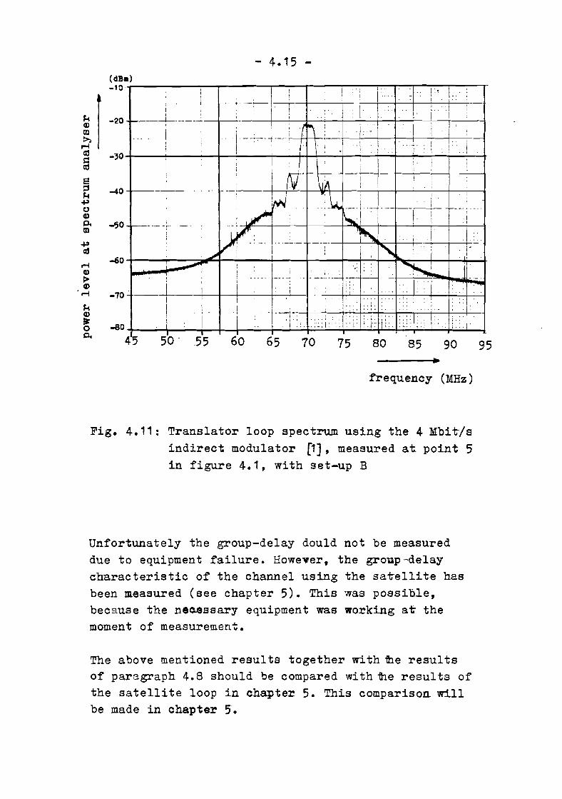
- 4.15 -

95908580757065

----r--.

45

-40

J i-' 1--- - r--+--~~,,-+.-----te--.:-.-+-I--I----i,-·~-60 +--........----:==--+-~-_+_--+-_:_.....,.-~_+_~lIr't-_+__+_+i___+

~ i " '~.,. .- ..- .. --i·~-- ----!-----+- ~r_.,...~..-.J

-70 . __-L.__-+i_+--+-_---I_......' _I I .: : . : :. ::: :: i . : : ....I 'I i ' . ;' :!. "[ i.1II' . I' I ·---~r~, .,.",; 1'1

-eo -;-__. -+-_---IIr--+--+-__+--.....I_._''+O:"";;...,j'i_I:.....:..,.:....ii....:.....i_Jot:· ': :_:.f-I ::..,:_::_:....:_:.-1:...i_.....·_·-i

5'0' .5'5 6'0

-50 - ,..--- -.-. +-

-20

(dB.)-1 0 ...--------:--.....,..~I--""T""~!-r---:---r-"':""::"':"":·i-~'""1'":"-;-~1.--,--:--,

, I t'f- - - t..-~--+--+---+--,-~-+-I-+---I---+-----,Itf-..--+---'-

I It!· '!' ._.-+-.---..l-t-~I --+----:...--+-.. +-!-'-+--+----i-+---+----+I-t-----lI i --;-c-' f"'\ I··I I, .['. : i . i

_30+----~----+-.;.....--+---..;_++_l-_+-....r --t-+--+--'-t'!-+-'~''---t1 •

I .

.__. .i-rv- llA: . I

,~. .·tl.d~---·· i'. --;8::s~~

oQ)

P­m~as.-IQ)

e>Q)

'.-I

~Q)

~oP-

frequency (MHz)

Fig. 4.11: Translator loop spectrum using the 4 Mbit/sindirect modulator ~], measured at point 5in figure 4.1, with set-up B

Unfortunately the group-delay dould not be measureddue to equipment failure. However, the group "delaycharacteristic of the channel using the sat-ellite hasbeen measured (see chapter 5). This was possible,because the neeessary equipment was working a~ themoment of measurement.

The above mentioned results together withfue resultsof paragraph 4.8 should be compared with~e results ofthe satellite loop in chapter 5. This comparison willbe made in chapter 5.

4.16

95908580757065

p:=.' __ T~q-l---:--t_ ... -: ....--q.- :~~~::c .':.

I, Ii 'I i I.l:_.. ·1' - :. -I ..-wI!

- .. I -:: _.. :..:. ~ ~ - -:: I ~: -: : ~_:: :::.

1---_. __.-

(dB.)-10 ......,----.,.----......-.----'1'""""--_-.,.-..,----,--.,..-.....,..--.,.-.,.-__

i ! 1- -:~ ;:: : ~:-+~~: :-:: :-~:: :::1::- ::=-:l~:-:~r----i--+-i--I--+-!,-'-..-_.-+----.-:-f:-:__-.:-+r-.• ~-~+.->-:_F-i-:=---.-~+-~-::-:_t-:-._-:1-:_-_.-:i;"':'.:'::":':_:....J:-~:...:-:-:._1-::--.:..J;:

~o

-40

-50

-70

-eo

Fig.4.12:

~

tn

r-lQ)

>Q)

r-l

F-ig. 4.1 J:

frequency (MHz)

~anslator loop spectrum using the diredt modulator(4 MbitIs modulation) [1], measured at- point 5int1.gore 4. 1 , with set-up B

frequency (MHz)

~r~slator loop spectrum using the 8.448 Mbit/s~nd~rect modulator, measured at point 4 of figure4.1, with set-up B

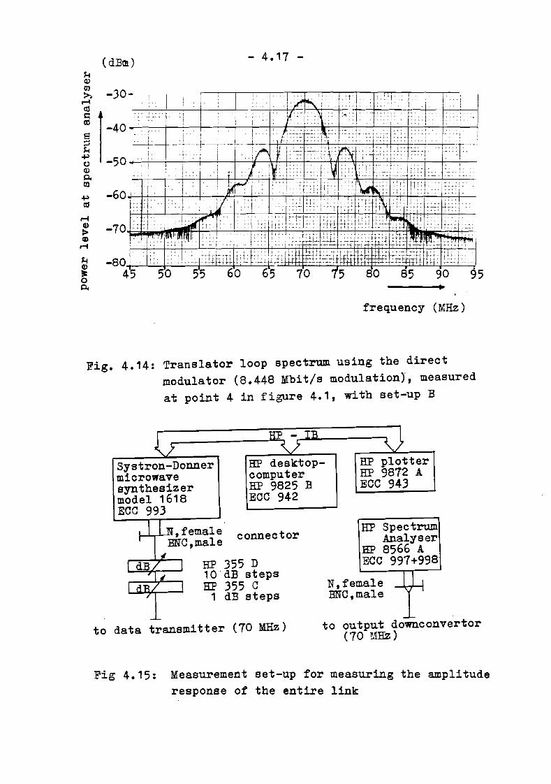
(dBC!) - 4.17 -

frequency (MHz)

Fig. 4.14: Translator loop spectrum using the directmodulator (8.448 Mbit/s modulation), measuredat point 4 in figure 4.1, with set-up B

Systron-Donnermicrowavesynthesizermodel 1618ECG 993

H

HP desktop­computerHP 9825 BEGG 942

HP plotterHP 9872 AEGC 943

connector

HP 355 D10"dB stepsHP 355 C

1 dB steps

to data transmitter (70 MHz)

HP SpectrumAnalyser

IiIP 8566 AECG 997+998

N,femaleBNG,male

to output downconvertor(70 MHz)

Fig 4.15: Measurement set-up for measuring the amplituderesponse of the entire link

- 4.18 -

Spectrum Analysersetting:

vide bw.:swp time:function:centre freq.:span:power level:ref. lev.:att.:

res. bw.: 100 kHz300 kHz

20 msecMAX HOLD

70 MHz10 MHz

1 dB/di'-5 dBm

10 dB

Fig. 4.16: Amplitude response of the entire link,usingthe translator loop

4.4. Link budget calculation

The initial calculations for the system at the EDT aredescribed in ~]. Although most of the values remainedthe same during the experiments, there are some differences.Moreover, some modifications were made after the firstexperimen~s; some of these values had to be estimatedinitially, because they can only be measured duringactual experiments.

a) By allowing spectral impuri ties to increase from 60 dBto 50 dB below carrier level and shortening some of thesemi-rigid coa::ial cabels, the outpu~ power of the T'tVT

could be increased; i.e., reduce the output back-offfrom 1.8 dB to 1.0 dB.

b) From the mea2ured satellite TWT curve (chapter 5),it w~s possible to estimate the output back-off of thesatellite T~T more accurately than before~J. In chapter5 it will re shown that this is a0proximately 1.7 dB

instead of 3.0 dB.

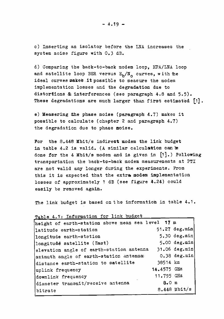
- 4.19 -

c) Inserting an isolator before the LNA increases thesystem noise figure with 0.3 dB.

d) Comparing the back-to-back modem loop, HPA/LNA loopand satellite loop BER versus Eb/No curves, with fueideal curves makes .it possible to measure the modemimplementation losses and the degradation due todistor~10ns & interferences (see paragraph 4.8 and 5.5).These degradations are much larger than first estimated [1].

e) Measering the phase noise (paragraph 4.7) makes itpossible to calculate (chapter 2 and paragraph 4.7)the degradation due to phase noise.

For the 8.448 Mbit/s indireet modem the link budge~

in table 4.2 is valid. (A similar calculsTion can redone for the 4 Mbit/s modem and is given in ~].) Followingtransportation the back-to-back modem measurements at PTIare not valid any longer during the experiments. Fromthis it is expected that the extra modem implementationlosses of approximately 1 dB (see figure 4.24) couldeasily be removed again.

The link budget is based on t he information in table 4.1.

Table 4.1: Information for link bude::etheight of earth-station above mean sea level 17 mlatitude earth-stat~on 51.27 deg.minlongitude earth-station 5.30 deg.minlongitud~ satellite (East) 5.00 deg.minelevation anele of earth-station antenna 31.06 deg.minazimuth angle of earth-station antenn~ 0.38 deg.mindistance earth-station to satellite 38514 kmuplink frequency 1.4.4575 GHzdownlink frequency 11.795 GHzdiameter transmit/receive antenna 8.0 mbitrate 8.448 Mbit/s

Table 4.2: link bud~et

Uplink budget calculation

Earth-station

1 HPA max power

2 output back-off

) feeder & filter loss

4 antenna peak-gain

5 pointing loss

6 EIRP

Propagation7 free space loss

8 atmospheric attenuation

9 propagation loss

10 eff. aperture isotr. rad.

11 power flux density

Satellite

12 antenna peak-gain1) gain loss at edge coverage

14 pre LNA loss

15 received power16 system noise temperature

17 uplink CiT

18 Boltzmann's constant

19 uplink CINo20 repeater noise bandwidth 21

21 repeater C/N (per carrier)

22 back-off (gain step setting)Downlink budget calculation

Satellite1 HPA max power

2 output back-off

3 number of carriers4 modulation loss5 post TWTA loes6 antenna peak gain

11.76 dBW

1.00 dB

2.46 dB

59.26 dB

0.2C! dB

67.36 dBW

207.36 dB

2.40 dB

209.76 dB

-44.56 dB/m2

-97.74 dB/m2

)1.02 dB

1.00 dB

0.00 dB

-112.20 dBW

27.9) dBK

-140.13 dBW/K-228.60 dBW/HzK

88.47 dBHz71.14 dBHz17.)) dB

0.00 dB

11.90 dBW1. 70 dBOpOO dB

0.00 dB0.00 dB

29.80 dB

7 gain loss at edge coverage 1.00 dB

8 pointing loss 0.00 dB

9 EIRP 39.00 dEW10 TWT carrisr intermodulation 0.00 dBW/K

Propagation

11 free space 108s 205.59 dB12 atmospheric attenuation 1.50 dB

13 propagation loss 207.09 dB

14 eff. aperture lsotr. rad. -42.88 dB/m2

15 power flux density 125.20 dB/m2

Earth-station

16 antenna peak gain 57.65 dB

17 pointing loss 0.20 dB

18 received power -110.64 dBW19 pre LNA loss (under G/T) 0.00 dB

20 system noise temperature 28.27 dBK

21 G/T 29.)8 dBK

22 downlink CiT -138.91 dBW/K

2) uplink C/~ -140.1) dBW/K

24 TWT carrier intermodulation 0.00 dBW/K

25 overall CiT -142.57 dBW/K26 Boltzmann's constant -228.60 dB/RzK

27 overall C/No per carrier 86.0) dBHz

28 bit rate 69.27 dBHz

29 Eb/No 16.16 dBDemodulation

30 Bit Error Rate target -40.00 dB

31 Eb/No theoretical 8.40 dB32 modem implementation 10S8 ).50 dB

3) distortions & interferences 1.50 dB

34 phase noise degradation (at P~.'0-4) 0.00 dB

35 Eb/No practioal 1).40 dB

36 margin 3.36 dBfor 99% of the time; two decimals tor calculation accuracy

•l\)

o

- 4.21 -

The link budget in table 4.2 is based on an atmosphericattenuation which occurs only for 1% of the time inthe worst month of the year [1] and which was certainlynot present during the experiments carried out in 1982.

4.5 Analysis of satellite adjacent channel interference

Care must be taken that any other users of the OTSduring our transmissions are not disturbed. One·therefore has to measure and calculate how much poweris transmitted into the other channels of the OTS.In figure 4.17 alI the channels of the OTS communicationtransponder are shown.

LINEAR LEFT - HANDPOlAR.Y 11794.864 CIRC. POLAR.

14J02.5

11MI,TRANSMIT SIDE - SPOTBEAM

1158Q.O 11700.0

- RECEIVE SIDE - EUROBEAM '"A"

142425 143625

MODULE A MODULE B - RECEIVE SIDE - EUROBEAM "B"

1445s.o 1446O.DI 14457.5 I

TC 4 ~x RL B12 14457.364 ~:g~~~~.

TC I 2' '4 ~CA1y LR B13 14457369 LEFT- HANDI . . ClRe. POlAR.

--'- - - - - TRANSMiTSlOE :EUROBEAM 77 - -11- - - - ---;RANSM~SIDE - EUR-;;;E~";- -

1149O.ll 115JClD 11575.D 11786.0 11792.5 11797.511510.0 I 11795.0 I

2' TM W:::x LR 813 11794.~9 R1GHT- HANDCIRC. POLAR.

11640.0

II 4 \ LINEARPOLAR X

\ 4 LINEARPOLARY

Fig. 4.17: Channel configuration of the OT·S [21].All frequencies in MHz.

The upper part of figure 4.17 shows the uplink·frequencY,or satellite receiver part. From this and fromfigure 4.4, 4.5 and 4.7 it is seen that only thetransmitted power in channels 4 and 4 of the OTS has

to be calculated, when using the hybrid ring switchingmodulator.

- 4.22 -

Figures 4.7 and 4.17 show which part of the transmitted,spectrum lies within channel 4 (or t) of the OTS. This'is the part with frequencies below 14.3625 GHZ. Becausethe spectral density diminishes at frequencies below14.3625 GHz (see figure 4.7) only the spectral densityof the transmitted spectra at 14.3625 GHz is measured.For this purpose the data transmitter is connectedthrough a 30 dB power-load (with a measured 29.57 dB,attenuation at 14.5 GHz) and a semi-rigid coaxial cabal(with a measured attenuation of 1.33 dB) to a Rewlett­Packard 8566 A spectrum analyser (figure 4.3). Withthis instrument, it is possible t~ ~ediatly measurethe spectral density per Hz bandwidth.The instrument was set as shown in table 4.3.

Table 4.3: ~pectrum analyser setting for spectraldensitv measerment.

spansweep timefunction

reference level 0 dBmattenuation '10 dBmarker 14.3625 GHz

power level 10 dB/div.centre frequency 14.3625 GHzresolution bandwidth 3 kHzvideo bandwidth 300 Hz

10 MHz30 sec

shift 11

Instrumentread-out(at markerfrequency) :

-120.0 dBm/Hz

Accounting for the power-load and semi-rigid cabelthis becomes:

N = -120.0 dBm/Hz + 29.57 dB + 1.33 dB = - 89.1 dBm/Hzo

Rurthermore.it is estimated that due to iransmit lossesin the 8-meter "antenna system another 0.5 dB is lost (,].

This gives:

- 4.23 -

The maximum transmitted spectral d..ens1..Q: in channel 4 ofthe OTS equals: -89.6 dBin/Hz = -119.6 dEW/Hz. Becausethe A transponder is designed for linearly polarizedsignals, channel 4 receives only the horizontal componentof the transmitted circularly polarized signal.

The maximum power flux spectral density, at the satellite,in chammel 4 (or 4) transponderband then equals:

dEW/Hz (+)

dE (+)

dB C-)dB (-)dB (-)dB ( -)dBW/m2Efz

(4-1)

transmitted spectral densityantenna peak gainpointing loss (minimum)atmospheric attenuation (minimum)divergency to satelliteloss due to receiving only one fieldmaximum power flux spectral density

-119.6059.260.000.40

162.71component 3.00

-226.4

For the actual maximum received power spectral densityone then finds:

maximum power flux spectral densityeff. aperture isotr. rad.antenna peak gain (eurobeam "A") [22]gain loss (minimum)maximum received power spectral density

-226.4 dBW/m~-44.7 dB/m2

29.5 dB0.0 dB---.,;..--.,;..---+

-241.6 dBW/Hz(4-2)

The system noise power density of channel 4 equals:

system noise temperature [21JBoltzmannts constantnoise power density (channe14)

A similar calculation for channel 4 gives:

28.1 dEE:

-228.6 dBW/HzK-200.5 dBW/Efz

(4-3)

+

- 4.24 -

noise power density (channel 4) -199.9 dEW/Hz .(4-4)

From (4-2),.(4-3) and (4-4) it is derived that themaximum received power spectral density of the signaltransmitted from~e EUT, is at leas~ 41.1 dB belowthe system noise power density of channels 4 and J ofthe OTS. Due to tthe rapid falloff of the transmitted.spectrum (see figure 4.7) this va~ue increases rapidlywith frequencies lower than the bandedge of 14.3625 GHz.

If the narrowband filter behind the earth-stations ~is removed, this value would still be more than 20 dB(see spectral measurements in (1]). A broadband filteris still needed (to remove intermodulation produc~s ofthe T'ft). If the narrowband filter is replaced by analready available broadband filter, fue available outputpower would increase 0.5 dB [1].

From the above it is concluded that. the, station at theEUT introduces no adjacent channel interference forthe other channe~s of the OTS. One could even :replace thenarrowband filter by a broadband one, merely increasingthe transmitted power.This is especially important because the uplink C/Nois seen 'to be smaller than 'he downlink C/No (paragraph4.4). So every increase in transmitting power will increasethe uplink C/No which means a significant improvementof the overall C/N •

o

4.6 Single Side Band (SSB) noisefigure measurements

The SSB noisefigure of the data receiver, withoutisolator and hybrid, has been measured with~e measurementset-up of figure 4.18. Measured are the SSB noisefigure

- 4.25 -

of the datareceiver without pre-amplifier, the DoubleSide Band (DSB) noisefigure of the data receiver withoutimage-rejection filter and pre-amplifier. All the abovementioned measurements were carried out without isolator.The&rived or measured SSB noisefigures are tabulatedin table 4.4. The SSB noisefigures are derived out ofthe DSB noisefigures by the following equation ~~:

Noisefigure meter Solartron .Magnetic AB, model 117 A video out oscilloscoopexcess noise: 15.6 - ex 1441 Eee 595dBsolid state ex 1441 Eee 59530 MHz input frequency ex 1443 Eee 5931 M1fz bandwidth noise source System

...Under 70 MHzEee 0907 r-- Magnetic AB

125 D Test ouput

SO dB

30 MHz HP 10514 A WG 31172/ Er=::il I d~3 dB~~ x L I

swept from 5,.5 dB 4R "90 to 110 MHz Eee 1845frequency generator .I~'"I - frequency counterRP 3200 B 17 dBm I I ED? model 548VHF oscillator HP 11652-60009 Eee 992

Eee 512

F~ 4 1S· SSB noisefigure measurement set-up...g. • •

noisefigureSSB = 2.noisef1gureDSB - 1

The results are plotted in figure 4.19.

(4-5)

Accounting for the increase in the SSB noisefigure dueto the isolator omitted (0.3 dB) and the losses of the8-meter antenna system (0.5 dB), the SSB noisefigureof the actual configuration becomes:

- 4.26 -

Table 4.4: SSE noisefi,.Qurestfreq. total without without without pre-amplesystem pre-ample filter and filter

M.l::fZ ;j;jJj ;j ;j.tl U;jJ:j .::l;;)l::S DSB SSB60 6.0 11.7 5.7 8.5 4.0 6.061 5.8 11.3 5.1 1.4 4.3 6.462 5.1 10.2 4.3 6.4 3.4 5.36} 4.15 9.5 4.0 6.0 3.1 4.964 4.6 9.2 3.8 5.8 3.0 4.865 4.65 9.3 3.9 5.9 3.0 4.866 4.45 9.1 3.8 5.8 3.0 4.861 4.4 9.1 3.8 5.8 3.0 4.868 4.4 9.1 3.9 5.9 3.0 4.869 4.4 9.2 3.9 5.9 3.0 4.810 4.4 9.3 3.9 5.9 3.0 4.871 4.4 9.3 3.8 5.8, 3.0 4.872 4.4 9.4 3.8 5.8 3.0 4.873 4.4 9.5 3.8 5.8 3.0 4.8

74 4.5 9.8 3.8 5.8 3.0 4.8

75 4.45 9.8 3.8 5.8 3.0 4.816 4.55 10.0 3.9 5.9 3.0 4.8

77 4.65 10.2 4.0 6.0 3.1 4.978 4.8 10.6 4.3 6.4- 3.1 4.9

79 5.2 11.3 4.8 7.0 3.4 5.380 5.8 12.5 5.6 8.0 4.1 6.2

noisefigure = 4.4 dB + 0.3 dB +, 0.5 dE = 5.2 dB(4-6)

varying only 0.2 dB in the band 66 to 76 MHz and whichis seen to be the best of all possibilities listed.

- 4.2.7 -

. ------- -_._-~ . -------------------------- ------------------_.:.._-------,,-----------~-

-------I-'l;- ----:------------------ --T-----T:---~:----j------r--F ;;:~::l.-

------~~- ~___;----_:_---~----~: --r--t- ; I., I: 1,--:---;I ,; I _ L -: _ -1 l' '-:1' •- -. _- I t

L ~f --------:----~-------- ----,-.:----~~--;-r---'--_-Tf_---'----'-i

1'-__-.'-:---T-- ! _

______:. :. 6P. '~_c -,-,_-~---,-_10---i1- l.'f.1 d' 7#.:-_~_------i...----'-_;1---

i" ; - --1-. •-t--. :f1~equen~y (MHz)·....-1_ •••__• __ ~_.__ __. 4 __ ·' " _~-_.- ••_-._- __.~. -... • ---.- ~_._, ,

_._~._----~---_._-- ---_:._-

-;--.....,.---------t--.-:-._- ..--.-----.--~:---t- ~: t. .

Fig. 4.19: Noisefigures versus frequency

4.7 Measurement of frequency st~bility and phase noise

T;he frequency stability of the various oscillatorswas measured with uhe spectrum analyser (see figure4.3). The instrument setting of table 4.5 was used.

Using the "peak-search" and "'A"-- functions of the spectrumanalyser it is possible to determine the maximumvariation in frequency between two sweeps, during 5minutes of measurement (100 sweeps). Using the "max-hold"

- 4.28 -

Table 4.5: Spectrum analyser setting for frequencystability measurements

reference level 0 dBmattenuation 10 dBmarkercentre frequencyresolution bandwidthvideo:bandwidthspansweep timefunction

at frequency of measurementat estimated average frequency

100 Hz300 Hz

5 kHz

3 secmax HOLD

function it is possible to measure the variation infrequency during the time of measurement.The results are shown in table 4.6, not includingthe local oscillator, which was already placed behindthe antenna. However, the most important result isthe stability of the 70 MHZ signal looped-back throughthe translator. Although these results are not excellen~

they are far below the maximum 20 kHz deviationacceptable for the 4 Mbit/s modem [24].

Table 4.6: Freauenc stability measurementsfrequency/oscillator time of deviation stability

measurement14.4575 GHz osc. 5 min -(100 swps) 75 Hz/3 s 2.10-tj 3s

2.6625 GHz osc. 5 min (100 awps) 7 Hz/3 s 3.10-9 3870 MHz received back 5 min (100 swps) 425 Hz/3 s 6.10-6 3s70 MHz received back 6 h (max hold) 3.46 kHz/6 h 5.10-5 6h

In addition Upper Side Band (USB) noise measurementsof the used oscillators and of the 70 MHz looped-backsignal are necess3ry to determine their phase noisespectrum. For this purpose the measurement set-up of

- 4.29 -

figure 4.20 was used. A special program for the HP­desktop co~puter was weitten and is described in AppendixG. If the USB noise of the spectrum analyser itself isnot exactly known, care must be taken to investigate

HP plotterHP 9872 AEGG 943

HE Spectrum AnalyserRP 8566 A10Q.HZ - 2.5 Gffz/2 - 22 GHZEGe 997 -f';' 998-

I _-----+-=HP::...." - IB I..I.... .> <.. .7c:=:=-----.....~ J.r------~----...... .-_.......;:w:;.._-..

liP desktopcomputerHI' 9825 BEGG 942

'0 ~N-connector,femaleto source

Fig. 4.20: Measurement set-up for USB noise measurements

whether or not one is limited by the USB noise of themeasurement instrument itself. To determine this, adata-sheet of the used spectrum analyser was used ~5].

The results of the various oscillators are shown inAppendices.G, D ~nd G. To explicit the formulas ofchapter 2, it is necessary to measure the USB noise ofthe looped-back 70 MF~ satellite signal. Also measuredwas the 70 ~rnz transmitted signal. The results are shownin figures 4.21 and 4.22 respectively, Comparing bothfigures, 'it is obvious that the measurement concerningthe looped~back signal is not affected by noise of thespectrum analyser itself, because the curve for thelooped-back noise is at least 25 dB above the measuredcurve of the transmitted signal. In ~6] it is shownthat this measured USB noise spectrum, L(f), can berelated to the SSB phase noise spectrum in the following

manner:

:>f - 0 (4-7;

- 4.30 -

In accordance with (2-23) it is no~ assumed that L(f)can be modelled on the following form:

Cl Cl ClL(f) 1 + 2 3 c :>

(4-8)= ""7 +-+ f - 07 f 14

where Cl through Cl are suitably chosen pQBitive1 4

constants (7] and where Cl is bandl1mited by :!tIlt and3

USB NOISE MEASUREMENT

-I: -- -- ~I -t=FH-i-- -m---- -, ----~ffH~--~-~~~[1~L(f) r-~ - .~-+--H+£ -1--- _I;=PL~

-3ll t---- --~ 4-- measured +--'-TtJ,-- +---i- i~I r, j ~! ! I I I, I I I L t J I I , ' I

-40 L-,-f- -! -i -i I t--- t ~! - t-j-i-t-l , -- --ll j' i -- r - -- -j .-,-~

-50 1- _.J -+ 't- --.. -- t I' ,- r-l--~ t--- I-------t -.j---~ I - I --, , --_8B~aPPrO~imation_-t_' I ~__ ..tl-r---~----+ ~_~ j. _~_ ~~

! " , " I l 'H -70L_L -J- i_I ~ - ~-- -1 -,~ '- --'--,~-f·~--+----,l ~j . ++-~ ~ I ,1, I ' , I" I I " "~ -98 ---t - --~ -L.-l f -- -'r' _. __J_ ! i I -- - - • t-·- '-_.•~" i: I . I : i: I I ,I ' I::

\ • I 1: 1 ! . ( I L I I 'J I-90 -+I--'-~ -ji·-j---,----~- i'-

I'- ;----1-1 -7-1---1 -f-r "-!' ;---' ---

I "l:±' ': i 'i ' L ",-100f--i---"r-f-j--" - --l'-r 11- -t- ---,--j---;-+---+-----, -j t, 1-· ,I I ' I I I' i '. I' I I I, i '

i-110 t-T-L:'-+r I -+, ~ ;-----1--- -t-l ;l----r-t-·l t t-- -~- - -;

-12111 -, -r-I HiI --1-+-/i·t -- -i---HI-I !-r-T --+-t-t-t -- i---+ .--

-13llt±±ttt=11'-1 - II t-+-H' --i ±±-'1+1 I-+t~, -- T- . -~-~-140 i--, "I - i-t--t---r-IJ -n----rTT1-15IJ . I _LiJ J.. .L....L...L_ _ J---'--J_.~.

1121 2 .." 811212 2 .." SUI· 2 .. e 1184 2 4 e- 81al 2 .. IS lUI-

F....qu.,.,cy. Hz ..

Fig. 4.21: U3B noise measurement of the looped-back70 MHz signal

C1 by Be (see paragraph 2.2).4 '. 4

On the basis of (2-23), figure 4.21 and the above,reminding that w = 2}{f, it is possible to estimate theconstants C1 through C4 (see table 4.7) and B

C•

The result is plotted in figure 4.21. 4

- 4.31 -

USB NOISE MEASUREMENTII

II

II

II

\

\

'\1\ n

iV\ ~A.A

~!v.-,-1111

-9

-I

-1118

-1211

~ -711

"-~ -."

L(f)

-1311

-148

-lSiIII 2 • e 81'" • e 81'" 2 • e 8111' 2 • e· 8111'

Fr-.q.....,.,oy. Hz

Fig. 4.22: USB noise measurement of the transmitted70 MHz signal

• . 'tl

!spectrum corresponding constants value

Cl20 dBcHza:::

1

Cl-10 dBcHz

Lef)2

C1-45 dEc

3C1

-83 dEc/Hz4

C1 41 dBrad~(2 Hz)~

C22

9 dBrad (2 Hz)

S~(w)C3 -35 dBrad2

C4 -80 dBrad2/ (2 Hz)

BC 100 kHz4

Table 4 T- Determined constants of L(f) and S (w)

- 4.32 -

The approximation differs from the measured curveespecially at low frequencies, so the phase noisecannot exactly be written in the form of equation(2-23), which is probably caused by the poorperformance of some parts of the upconvertor andwhich is discussed in Appendix D.

Assuming {i'M\ of (2-46) t.o be equal tto -3 dB [7], [1 OJand determining C/No = 83 dB from figure 4.21 (take ~t

1 MHZ, at which f'requency the phase noise can beneglected), it is possible to determine the degradationdue to phase noise.

Because (2-67a) isfrom (2-15):

" [vM<ciINo )]

G [2l<3C 4 ]

valid for these values, G is obtained

!:! 0.48

this corresponds to c = c(~) ~ 0.35 (table 2.8). Fromtable 2.8 one then obtains:

F :! 0.85

And from (2-43) and table 4.3:

BL ::t ~.1 00 kHz e:: 285 kHz (4-11 )

Substituting these values together with the values forC1 through C4 (table 2.8) in (2-41) and taking BIFequal to 1.5 times the data rate [20]: i. e., Z 13 MHz

it is possible to~termine the total phase jitter:

(4-12)

- 4.33 -

or:

(4-13 r

With (2-54) the average probability of error due tocycle skipping can be calculated:

1( -lrPecs = '4. exp 2

32. O'J6T(4-14)

The degradation due to phas~ noise can now becalculated as follows. Assuming a BER t~get of 10-4

(corresponding with 99% of the time see paragraph 4.4)a theoretical E/No of 8.4 dB (see (2-55) is needed(the extra needed 0.4 dB for Differential~codedQPSKis to m accounted for as modem degradation in ihelinkbudget of paragraph 4.4).Due the BER target a~ 10-4 means that the probabilityof error contributions from thermal noise,must be lessthan 10-4• From (4-14) the probability of errorcontribution due to phase noise. equals 2.3 10-8 whichis much smaller than the BER target of 10-4 and thereforecan be neglected. The degradation due to phase noiseis therefore considered to~ 0 dB. Note tha~, the abovedefined degradat.ion due to phase noise depends on t,hechosen BER target. However, ~cause the Q-function of(2-55) is such a steep function for small error ­probabilities, the degradation will always be smallunless the desidered BER target is ne~r to or smallerthan the probability of error due to phase noise. Aprobability of error which is smaller than the probabilityof error due to phase noise can never be achieved.

In table 4.8 the ~gradation for various BER targetsis given:

- 4.34 -

Table 4.8: Degradation due to phase noise for various-8 .

BER-target~ (Pees = 2.3 10 ) for DPSK.

BER- target degradation

10-5 0.00 dB10-6 0.01 dB10-7 0.09 dB10-8 ~ (not possible)10-9

00 (not possible)

4.8. BRa versus Eb/No curves

A good insight in system performance is obtained fromthe measured HER versus Eb/No in comparison with theideal curves. The measurement set-up used for the8.448 Mbit/s modem is described in [20], so onl;ythe final results of these measurements will be givenhere. Also, the standard curves for ideal ~modulationswill not be derived, because they are given in manybooks [27].

(4-15 )(DCQPSK)

For the 4 Mbit/s modem the ideal curve is that ofDifferentially Coherent :~PSK (DCQPSK) [27]:

Eb-rP = 1 e ae ~.

For the 8.448 Mbit/s modem the ideal curve is that ofCoherent QPSK (CQPSK) times two because it- uses differentialencoding and decoding [20] (see 2-55):

(4-16)

- 4.35 -

These curves are shown in figures 4.24 and 4.25(subsection 4.8.3.).

Tne back-to-back 4 Mbit/s modem loop (possible onlywith the indirect modulator at 70 MHz) was measured.with the measurement set-up of figure 4.23.

4 Mbit/s clock HP Data Generatormodulator HP 3760 A EC 1G

2 MHz clockword1ength: 215_1

70 MHz -t Pseudo-Random [24]Data Ge~erator ~word1ength: 232_1

pseudo-random data

~~ Noise Generator,r System (24)6 dB power-splitter

clock

[!J,

filtered 70 MHz out lIP Error Detector, liP 3761 A

4 Mbit/s -EC 2Gdemodulator pseudo-random data.-

Fig. 4.23: Modem back-to-back loop HER measurement set-up

The measurement set-up of figure 4.3 was used to measura

the s~gnal and noise power after the IF receive filterof the demodulator. First the powers~litter wasdisconnected froml;;he modulator and matched with a 50.nload. Then the filtered 70 -;"IHz output was connected t:othe powermeter and the noise power N was measured. Thefiltered 70 MHz output was then connected to the spectrumanalyser and the one side spectral noise density No

- 4. J 6 -

was measured at the filter centre frequency. Becausethe equivalent noise bandwidth BN equals [28]:

N=No

(4-17)

it is' possible to derive ~. For the 4. Mbit/s demodulatorit was found that:

BIF (4 Mbit/s) =~ = 5.4 MHz (4-1-8)

For every point of measurement the following was done~

The power splitter was disconnected from tthe noisesou:rce and matched with a 50!t load. After this, themodulator was connected to ithe power splitter and thecarrier' power C was measured at the filtered 70 1iliz

output: of the: demodulator. Then the modu1..atar autputwas disuo·nnected from the power spli t.ter· which was mailchedwi th a 50.!t load and connected to tthe noise courca ..The. noise power was measured at the' filtered 10 rJHzoutput •. Substituting this value t'ogeilher- wi trh (4-18)

into \4-17) gives No. From thes.e. two results we obt-ainC/No • Dividing by the nuinber of bits- per second

(4.106) gives Eb/No,. Then the modulato'r was againconnected to the power splitter' and the correspondingBER was measured.The measurements concerning the 8.448 Mbit/s modem aredescribed in [20].The results' are tabulated in table 4.9 and shown infigures 4 •.24 and 4.25 (subsectio,n 4.8.}).

As already mentioned the 8.448 Mbit/s modem did notperform as well as before transportation to Eindhoven.However, it is expected that the extra degradationcan easily be removed. again.Comparing the back-to-back modem loop curves \viththe corresponding ideal curves makes it possible todetermine the modem implementation losses at the

- 4.37 -

T~ble 4.9: Back-to-back modem loop BER versus Eb/No4> Mbit/ s

Eb/Uo (dB) Fe at PTI at EDT-

19.1 4.2 10-9 EclNo (dB) Pe Eb/No, (dB, 1'e.10-a18.2 4.4 .

17.2 3.0 10-7 14.2 7 10-7 16.1 4.10-7

16.2 1.5 10-6 13.2 6 10-6 14.7 3010-6,

1.5.2 9.' 10-& 12.1 8 10-5 13.1 3.10- 5

14.2 5.) 10-5 11 .0 3 1,0-4- 12.7 1.;10-4

13.2 2.1 -4- 10.0 8 10-4 11 .5 8;10:-4 '1012.2 7.3 10-4 9.1. 4 10-3 9.7 2.10- 3

11.2 1 .9 10-3 8.2 8 10-3 8.5 9.10-3

10..2 ~.1 1d-3 8.3 1.5 10-2

9.3 1.0 10-2

threshold bit error rate of 10-4-. The .results are- shownin table. 4.13 (with and without including the extraenergy needed in comparison with CQPSK) in paragraph 4.8.3.

Since the threoretical Eb/N o of 8.4 dB applied in. thelink budget of paragraph 4 .. 4 corresponds to CQPSK, thedifference with differential encoding/decoding is includedin the link budget of paragraph 4.4 (see table 4.13in paragraph 4.8.3).

From figures 4.24 and 4.25 it is clear that both curveshave the same general form as the ideal curves, so themodem implementation loss is practically independentof the probability of error o

In order to predict the systems performance during theearth-satellite transmissions, the translator was built

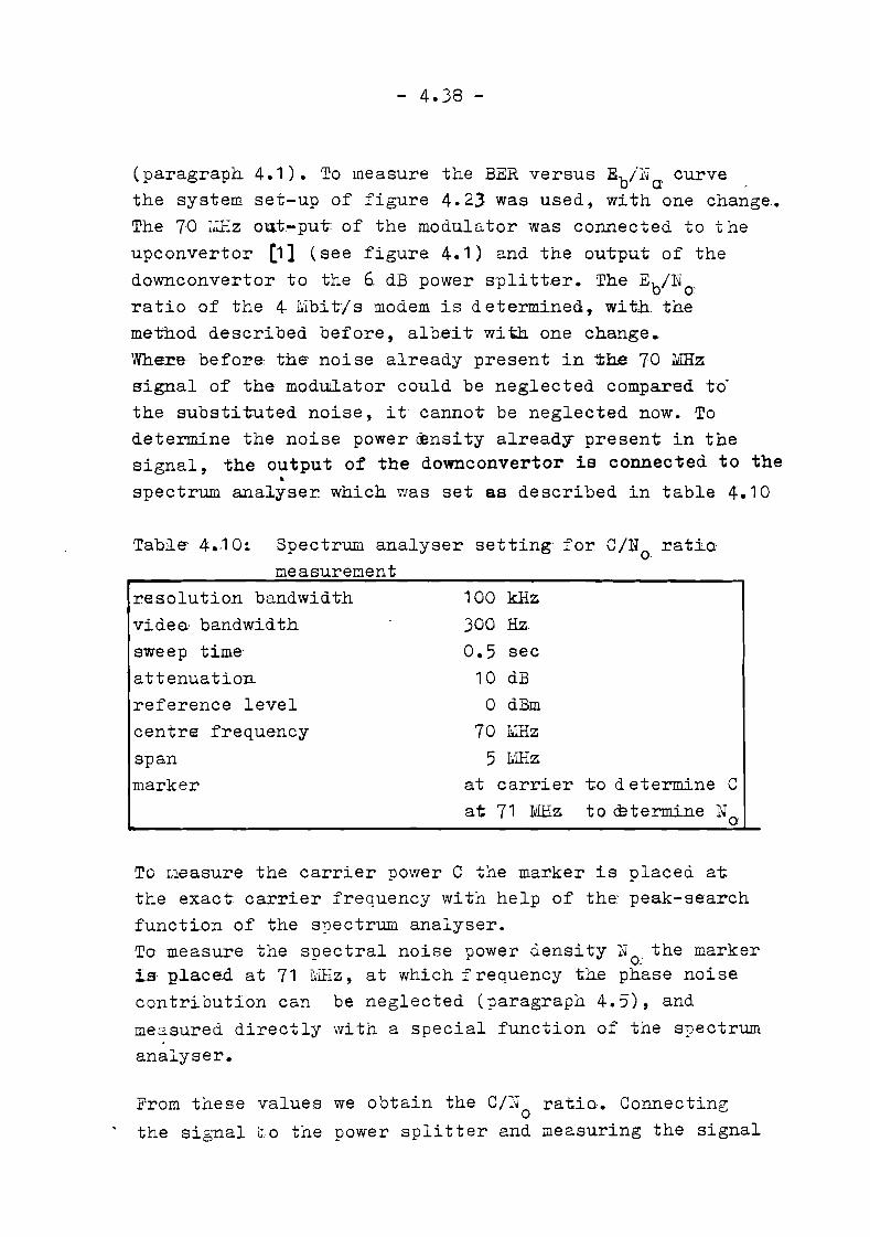
- 4.38 -

(paragraph 4.1). To measure the BER versus Eb/N cr curve.the system set-up of figure 4.23 was used, with one change.The 70 ~liliz out-put-: of the modulator was connected to theupconvertor ~1 (see figure 4.1) and the output of thedownconvertor to the 6. dB power splitter. 'rhe Eb/Noratio of the 4 l'ilbit/s modem is determined, with. themethod described before, albeit- with one change.Where before: the:- noise alre.ady present in -the 70 MHzsignal of the modulator could be neglected compared tothe substituted noise, it cannot be neglected now. Todetermine the noise power rensity already present in thesignal, the output of the downconvertor is connected to the

•spectrum analyser which was set as described in table 4.10

Table: 4.·10: Spe:etrum analyser setting for CINo rat.i.omeasurement

resolution bandwidth 100 kHz

videa- bandwidth 300 Hz

sweep time 0.5 secattenuation. 10 dBreference level 0 dBmcentre frequency 70 MHzspan 5 MHzmarker at carrier to determine C

at 71 :MHz to cstermine No

To ~easure the carrier power C the marker is placed atthe exact carrier frequency with help of the peak-searchfunction of the spectrum analyser.To measure the spectral noise power density No: the markeris placed at 71 r.iliz, at which frequency the phase noisecontribution can be neglected (paragraph 4.5), andmeasured directly with a special function of the s~ectrum

analyser.

From these values we obtain the C/l:J ratio. Connectingo

the signal t:o the power splitter and measuring the signal

- 4. 39 -

power at the filtered 70 li~Hz output of the demodulatoras before, makes it possible to calculate C and ~ from'

othe signal itself. The spectral noise power density ofthe substituted noise is measured in the same way (seetable 4.10 and figure 4.23) and from this the total noisepower density can ba'determined. Then EblNo can beQ.&.].culated and the; corresponding BER can be measured.Similar, the roasul ts f or the. dire:ct modulation areobt"a:ilne.d .. The me.asurements concerning the 8.448 IUbi tlamodem are descrihed in [20]. The results are tabulatedin table 4.11 and. shown in figures 4..24 and 4.25 ..

Comparing the HPA/LNA loop curves with the. correspondingba<t:k-to-back modem loop curves makes it possi.ble todetermine the degradation due to distortions & interferencesfor the indirect modulators at: the threshold BER of 1.0-4 0

IJ:ii. tially these values were substituted in the linkbUdget of paragraph 4.4, but later on, ~hey were replaced

by the values obtained from the sat:ell:ite e:xperiments(paragraph 5.5) .. The results are tabulated in irable 4.12.

For the direct modulators it is impossible to measurethe modem implementation loss snd degradation due todistortions & interferences separataly, because it isimpossible to m?ke a back-to-back modem loop. Comparisonof the aboTe menti.oned curves with tne iaeal ones makesit possible to ~termine the total amount of degradation.The re suIts are tabulated in table' 4.13.

In figure 4.24 the back-to-back modem loop and HPA/LHAloop curves of the 4 I'i~bitis modem and direct modulatorusing 4 ~ilbi tis modulation are shown. Due to equipmentfailure, the satellite loop curve could not be measured

(chapter 5).From this ttloss varies

This will be doneis obtained that,from 4 dB at Pe =

in future experiments.the modem implementation

-3 -710 to 5.8 dB at Pe = 10 •

- 4.40 -

Table 4.1.1 EPA/Ll~A loops BER versus Eb/H o

4 ~llbi t/ s 8.448 ~wlbit/ s:iindue.ct direct indirect direct

Ell/No Ee E jN J?e ~~!lJc Pe Eb/Hc,pb 'c e

<,dB1 ' '

(dB) UrH) ( oR)

21.0 8.3 10-9' 20.7 2.1 10-8 ..)17.1 2 1,0-6 17.2 3.10-7

10-6 10-6 10-6 11.1 3 -117.3- 1.0 17.2 1 0b 16.7 5 10 "

18.4 4.1 10":7 16.6 ~.4 10-6 16.5 6, 10:-6 16.4 5 10-7 .

1.7'.9 8.3 10-7' 16..0, ~.8: 10-6 15.8 1 10:-5 16.2 8 10-1

10-5 10-5 1.4 1)-5 14.7-6

16.8 1 .2 15.3 3.5 1503 ITo 10

16.1 1.8 10-5 14.6 2.1 10-4 14.9 ~ 10-5 14.2 2 10-5

1.5.7 2.6 10-5 1306 3.0 1Q~4 14.4 " 10-5 13.8 41 10~5

1407 -5 13.1 7'.,4 10-4- 13.9 9; 10-5 13,.1 l' 10-49.310-

13~91 2.6 1Q-4 12.2 1, 09 10-3 13.0: .3 10-4 1i2.5 2 10-4

1 J..1 6.5 10-4 11.3 '301 lU-J. 12 0). 6; 10-4 11.6 6 10-4

12..2 4.5 10-3 10.4 "l05 10-3 11 08 2. 10-3 10.a 1.5 10-3

11..4 8.3 10-3 9.6 ~.2 10-2 11 .1 ~, 10-3 9.7- 4 10-3

10.4 1.5 10-2 10..0 l5' 10:-)' 900 6 10-3

905 ~ 10-3 8.0,1: 10-2

8 00 ~ 10-2

8 09 ~ 10-2

Table 4.12: Distortions & interference levels for theindirect modulators, using the translator'loop (at Pe = 10-4 )

modem distortions & interferences

4 Mbit/s 1.0 dB

8.448 IvIbit/s 1.3 dB

Furthermore it is obvious that the difference betweendirect and indirect modulator is less than 0.3 dB.In figure 4. 25 t£~e back-to-back modem loop, HPA/LNA

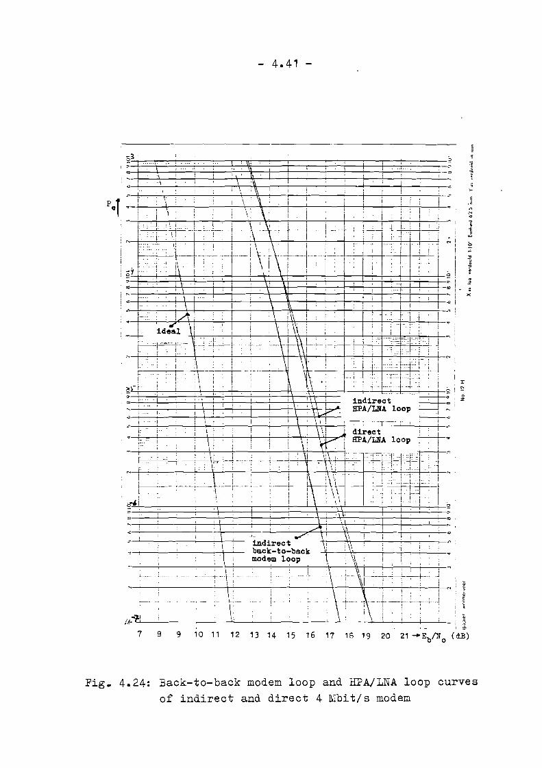
- 4.41 -

"",

0 -=;;-

1-¢ ;

>-

i e•<

i '"i

N

t· -0."

J;;

---r 1... "T : ~

i."

~l..

a- 2<Xl ;

>(

-0

., iI

i

!

\ '\\

, 1\;

'\ i\\

I·

,....,.---,..... ~. ! ...:

, i

: \ , ' \ 1 i

1- ..r-··1-',

I ~ t-<Xl .... , r,

i E:-c'::.! A .: i \ t \\ II~.. I ... \ I.' ,I. \ i, \\ I, Ii:"'-t ideal ,"*..".."..,-.+,',-:-i----;--+----;--t---f-,_\+_\-t-_,__+-_,__+--+--+--,...'---I--L...<---;-----'-

i f'---.·. :c!I.~.··~... · ..I.,·.-.:;~ ..-,li~':-"'- .• l! '11._. ~I_ll,~,.'--It,--:.---+-~I---'-.;---4---+:'''''·~::.f--,:.:j--.::..:·'+-'-' ~I -r \\.1: ,"I.....fl., , \ '-J\I--\-1*".----1!---:.-~'-+--:+1.:::...:.. t::.:.::::+-:-';'::::-+':.:.:j.::'---+--:-.''----1

f- . I '1-;-r----·t-··-t-·.... [. I '\ i 'I, :,.! \ i ... ,r:. :~::::l

, ~~-~. I I . : :' r t I \ \ ':. •.• ,:1:···1 . , I .

i ;-+__----J.--+--'---'-;-.;...--;....I---'----'---++--,-,-1-1-.-.-;.-. indirect "'F=F: :-+---;-I.--+-_..J.....-\-,+-,--+--+--+--+-\+\---li-'\-\\'~"-~-+'-,;L HPA/LNA loop q=~

-0 .. '1 , : i I \ f \ \ ! - ...1'-:--] r----r--o\ ! \ l \ If 1 direct Ll."\ i \ ! ~ i HPA./LNA lOOp! ! ..

f:- , j.--l----c-c..lb-'-i -. i -'-- ~-.._,~ ·~.JL~'~L: r~.· :-:':~'~"':J~c' ~·i ..,j' . . ;.; Ii : : 'T I: I ; , . \ \: I· ; : ,·;1 'l

~j,-_·---;-~1·~--j·---l··· f'-1---~t\\1-' ~·I' iUi ..i" i! i::' i ; I i\ I \ \ i .:;' I I . I 2

",'=======::==+==:==t====t==:::t:4==::=t¢::=P==±=±=±:"""':-----+-----~-j--,---i----'---i-----'--+-+--_+"---_i___,__tT- ..-.-l--:-:-,""";,-<Xl .

, \ i.A i \;\----'--..,------:..---'---,+\~-""".L-. ........;.---'----:7£......1\ri-----'+\-I-"---1-....L.--:~-+-_'~, -0

: \ indirect !,'\\back-to-back

;\ modem loop \ t, \~\ i '.. . I

1--. _

8 9 , 0 "

;. \1._,_.+-'Li..~..:..~I' ,I I ,

;, I'! i !, I

Fig. 4.24: Back-to-back modem loop and HPA/LNA loop curvesof indirect and direct 4 Mbit/s modem

- 4-.42 -

- ?I!IJJfL

--..---------------~-- ----

----,--,--,---,--\-------,--

indirectsatellite

r loop

--=========~$~$~=====-

--~-------\--------_t__--+++_-.--J\;___...;....--,--;-----:..~~-......:......

indirectHPA/LNA -- -,-loop

t ---------.---Jf-------\-----+--L~~-------+-

"-.i0'C

12 13 14- 15 1610 11987

/b--;~----'-------__l_~_____:. ~ ---__~_~_~

Fig. 4-.25: Back-to-back modem loop, HPA/~NA loop andsatellite loop curves of indirect and direct

8.4-48 fubit/s modem

- 4.43 -

Table 4.13P ~easured implenentation loss (plus degradationdue to distortions & interferences for direct modulatiotl)at, Pe =- 1lO;-4 (Ilee.. f:i:~s 4.24 and 4.25)

mO'dem loop mod. loss+degradation (dB) describedcompared compared on page

to ideal to CQPSKcurve ideal curve

back-to-back ;nn;,... 4.5 5.4 4.37&4.384 iYlr!i.,.. 5.5 6.4 4.40)[bit/s .H:PA/LNA 5.5 6.4 4.40 -

directback-tt"\-back ; nn; ,.. ... 3.1 (+0 0 8) 3.• 5 (+0.8) 4.31 & 4.38

;nn;1". 4.4 (+0.8) 4.8 (+0.8) 4.408.448 HPA/LNA dire'ct 3.5 (+0.8) 309 (+0.8) 4.40Mbit/s

4.6 (+0.8) 500 (+0.8); Yln; .,..

satellite direct 4.4 (+0.8) 4.8 (+0.8)

and satellite loop curves of the 8.448 Mbit/s modem anddirect modulator' using 8.448 Mbit/s modulation, are shown.The demodulator was adjusted for' direct modulationduring these measurements.

From figure 4.24 it is obvious that the direct modulationcurve has the same form as the back-to-back modem loopcurve. The modem degradation (back-to-back modem loopmeasured at PTI) varies from 2.5 dB at Pe = 10-3 to302 dB at: Pe = 10-6 • Experimental results have shownthat the HPA/LNA loop results using indirect modulationcan be improved if the demodulator is adjusted for thistype of modulation~O].

Comparison of the H?A/llfA loop and satellite loopresults will be done in chapter 5.

5. SATE~LITE 100~ EXPERIMENTS

In this chapter experiments carried out during 1982 atthe: Eindhoven University of Technology are described.During ~hese first sessions only spectra, amplituderesponse, group delay characteristic, BER versus Eb/Noand the satellite's power transferfunction wereme:asured. The results and comparison. with the results0-£" the translator loop are. discussed in this chapter.

5.1. Satellite transferfunction

Each measurement session was" started by checking theloo~erl-back carrier frequency while transmitting aunmodulated carri.er with reduced power. To determinethe frequency, the data receiver signal was connectedto' the spectrum analyser (see figure 4.3) and thetransmitted power was increased to a value just sufficientto get a reasonable instrument reading. Then the LO­frequency was adjusted ~o get a rece'ived-back carrierfrequency of 1(0 MHz +/- 100 Hz o

Thee actual transmitted power is 0.5 dB lower than thesignal power connected to the "8-meter antenna system"(see figure 4.1) due to coupler and feeder losses of theantenna system. This 0.5 dB was accounted for under"feeder &i filter losses" in the link budget (paragraph

4.4).

Just before each me:aaurement se:ssion the transmittedpower was accurately determined by measuring thesignal power of the si.gnal connected to the antennasystem and substracting O.J feeder & coupler losses.The signal power of the signal connected to the antennasystem was measured with the measurement set-up offigure 5.1. Correcting for the 29.57 dB power attenuator

- 5.2 -

power-load Power SensoT Power Iii-eterliP 8481 A I-- liP 436 AdB ECC 918 A ECC 918

29057 dB

signal14.4575 GHz

Dat-a

Transmit"ter 1 dB steps: 1,0 dB stepsliP 355C Hi' 355 D

~ J1 7(0 MHz crystall/dB : /dB o'scillator, ,

Fig. 5.t: Measurement set-up for measuring t;hetransmit~ed power

and sUbstracting the 0.5 dB feeder & coupler losses, theactual transmitted power equals:

Pt- = instrument read-out (dBm) + 29.07 dB (.5-1)

Attenuating the 7,0 Niliz signal in 1 dB steps and measuringits corresponding transmitted signal power level, makesit possible to transmit a unmodulated carrier withdifferent, well de~1ned power levels. Starting at a lowpower level and increasing the transmitted power in well

known steps and knowing the earth-stations receiverresponse, makes it possible to measuxe the satellitepower transferfunction. For this purpose the receiverresponse was calibrated. Increasing the attenuation ofthe precision attenuator, at the 11 GHz level in thetranslator loop (see figure 4.1), wit-h 1 dB steps andmeasuring the output level at the 70 ~~z leval, makesit possible to determine the receiver response. Theresult is shown in figure 5.2. 1dB increase in inputpower corresponds with approximately 1 dB increase

in output power (linearity).

- 5.3 -

With this calibration the satellite power transferrunctioncan be measured. The result is shown in figure 5.30

( d Bm~)~""""""-'--'-""""""''''''''''''''''''''''''''~''''''''''''''W''T'"C"".""".==--r-r-rT'''T'''''''''''''''''''''.....-T''T''T''rT'''T....,-r'1'''-r-iT~'''T"T"''TI

t.

11: ···I··T .. ++ .....': 1.:';:.. ·.•. 1':':,:::.;"+"-1 "1 ' 1· ·1 .. + i IJ i ; . i ;

~ . 1..\.. ' .>+:.. .I!: .', a~/:: .,.-' i' T II'!! V1--t.llff I :!: :::' ,.. ..·1·· .. ·. 'c;' ';': .;:.." .' H:;' ~~ +··1 !! .! I j ~.!: : i..- 4-~Tr-1->, '! .. ~ i·· 1- 'f-" "', ,; "~g: '.~ i ~··I . '!. 1 Ii' I V i I u.,' I • ~

r-I -,~ I" --+ -i' ..,I-J-as ! . "j -\- ",'+'" ri , I,.. .+- ,. : !. Iii l/:. 1 ! t:L I : I Is:: ".+ : . I V -l- H if- -- -\ +-" .._- "r- "l"'~- 'Ias 'I" .i i L·I ...... -. t . i, ~.v- _'- .: 1~ .1 ',' . ~ "j'- ! "I' ~!. i ._~..Ja ,I', • j "I ,.' Vi I ",~ .',,1:':. I·" ,'" I'" I; ~..... ~ +4.-1-+fY .:-l~- ··j-·_·I :'1

j., ',' . . i "'+1

i ~:; .~.+"-rl':-+-i-i, " : r"i :. ~~Dtt:Lj'~r':ill j ';'"'j '}~,1,'p, I l" i: i ! I· ,.. I , i I : >, , ' , I J 1 I 'I

a:I -10 r-',-l,.......!I-.l-:-r·:-r I : I' I"!; _. - '-"t ,.~ -I : 1,. "" i' .·l i :.- 1..., '1/ f.-·n' ' : i : .. ,-- , '.':' -~ ...- I-T·-t-·- L,. . . i .. ,. .,-ias I i I ! . .! .'. I i ·1 I l7 ii" :, j: : I I : I!!

-II i-t i: ' . r I I ! I I Y .... -N',.. +.-j-.... .. r1-', ... :..... -! ,. \ "', :.!: ! ...'t·~1

~ _~JffiijI ! Ii' I 1,--j'l I E.' 'Vi': ' h-~-~-H--;J·~_ .. ~ l~ i j ~'I -: l ..11';1,

~ ,I' 'II," i." :,' i . i" i.v: I". 'I' +--:- !-\-I -,+:- -7- ~ I ;-1'II j., \1 i '-r ~~r-I -a-!' i,! : 'i" 1:'17 ..· .. ·"1 : _:_+:._ ..... f-J... -_.~- .... - "'r j ; -i I .-.~-j

i :; j~-_;ii).i~0:+,·~I.L~+·:.·. i- :; :+iIJjrrt'n~F~:"...tJrl~~11--.',,1!· ·'t:"t~~,·t'~,... I.... .1",. -' T.l-·c ··F h -I'F>. . ..~ .. ··1·1· il I j i' I . I ' l " ., J- -18 '1', .... ' '."".::. ., ".. . '..... " I 4 }-'-I- _".. ,,0_,-" ;"...,.. , ~ _.-'-

I, ~ ,r" '" '\ 12 II '0 'I 6' t 1- ,- • J ~ , 0 •

extra attenuationof precision attenuator (dB)

Fig. 5.2: Receiver response

The saturation effect of the satellite channel isclearly seen. Extrapolating the measured curve withhelp of the ESA curve (see figure 504) enables one toestimate the output baCk-off of the satellite TWT. Infigure 5.3 this is seen to be:

output back-off satellite - 0.7 dB ( 5-2)

This value plus 1. dB, due ta the reference of 1 dBoutput back-off in the ESA-curve (see figure 5.4),is used in the· link budget of paragraph 4.4. is 1.3 dBcloser to saturation than first estimated. This is'

caused due to lack of very accurate.. data a;f the satellitepower transferfunction. During all the experiments the

5.4 -(dBm)

-r 1:'"

r. --... I

- -_.~ -t-Q) .... -m -,~r-f -,

L1l

a .....s::s .(~

~ofo:l -I,0Q) ....~m

ofo:lasr-fQ)

:>Q)

r-f

J.IQ)•0~ - _r' 0

IJh~lh

10 .,signal power connected to antenna (dEW)

Fig. 5.3: Satellite power trans£erfunction (channel LR,gain step 6)

Or-------''------......----.......... .......... .......... --.

I --

LJ..:lJ..o::>l::U<!CD

f­::)0­f­::)o

2

6

8 x

x

173. 1978

RESULTS 'X' FROM PRE - LAUNCHMEASUREMENTS WITH 80 BEACON OFF

-120 -115 -110 -105INPUT FLUX DENSITY. dBW m-2

-100 -95 -90

Fig. 5.4: Dynamic range of channel LR at saturation(gain atep 15) [291

- 5.5 -

satellite's TWT is driven near into saturation i.e., at·0.7 dB output back-off.

5.2. Amplitude response

To mea2ure the amplitude response of the entire linkusing the satellite and without the hybrid in the datareceiver (see figure 4.1), the measurement set-up offigure 4.15 is used.Again the program described in Appendix G is used tosweep the synthesizer. The result is 3hown in figure

5.5. spectrurr.analyser setting:

res. bw. : 200 kHzvide bw. : 300 kHzatt.: 10 dBref. lev.: -4.0 dBmspan: 10 fLHzswp. time: 20 mseccentre freq. : 70 I'{Hzpo',\'er lev. : 1 dB/divefunction: max.HOLD

?ig.: 5.4: Amplitude respon~e of s~tellite looped-backexperiment.

Probably due to driving the satellite's TWT into 3~turation,

is the amplitude r~s=on8e of the complete ?~tellite loopflatter than the ~m:litude res~onse of the local translatorloop (see figure 4.16). From figure 5.5 one C2n see thatthe amplitued varies le2s than 1 dE over a 10 ~Hz range •.• lso measured is the am~litude response of the satelliteloop w~2n the satellite's TWT was driven at 2 and 4 dBextra output back-off (as measured at the centre of the

- 5.6 -

band, i. e., around 70 ~,~~{Z). Th is 'N~i3 done in a 30 1:Hz spanand with a slightly different program for the synthesizer(see Appendix G). The results are shown in figures 5.6,5.1 and 5.8. Obviously, the amplitude characteristicchanges significantly when the output back-off of thesatellte's T~~ is changed. This shows major linearvariations of the amplitude response are located beforethe limiting elements (TWT) of the satellite.

max.

spectrum analysersetting:

100 kHz300 kHz10 dBo dBm

)0 MHz20 msec10 MHz

10 dB/d

res. bw.:vide bw.:att. :ref. lev.:span:swp time:centre freq.:power lev.:function:

Fig. 5.6: Amplitude response of satellite loop (0 dBextra output back-off, 30 MHz span)

It is interesting to check whether this is atributableto the transmitter or the satellite input.

5.3. Group delay response

In order to measure the group delay response of the wholelink using the satellite, the measurement set-up offigure 5.9 was used. The equipment was not 'in perfect

- 5.7 -

spectrum analysersetting:

as in figure 5.6

Eo beacon

Fig. 5.7: Amplitude response of satellite loop (2 dB extraoutput back-off, 30 MHz span)

spectrum analysersetting:

as in figure 5.6

BO beacon

Fig. 5.8: Amplitude response of satellite loop (4 dB extraoutput back-off, 30 MHz span)

- 5.8 -

shape. Some functions did not work anymore (e.g. loopbandwidth adjustment of the receiver). Due to this andprobably due to the poor phase noise performance of thelink equipment (as discussed in chapter 4), the measuredresults are not very accurate and reliable. In figure 5.10the measurement read-out when the transmitter and receiverof the measurement equipment are connected to each other

TransmitterHP 3710 A IF-BBHP 3716- A

ReceiverHP 3702 B IF-BBHP 3705 A

1-----t+75Sl/50..a.:.....--....70 MHz totransmitter

75Sl/50AI4--70 MHz fromdata receiver

span: 10 MHzdeviation: 300 kffzBB modulation 500 kHzcentre frequency: 70 MHz

Fig. 5.9: Measurement set-up to measure group delay

for calibration. The noisy group delay response of thesatellite loop is shown in figure 5.11. It is stronglyrecommended to measure the group delay response again,after the phase noise performance of the equipment issignificantly improved, or more suitable equ~pment

is available. However, if an average curve is estimated(see figure 5.11) it can be seen that it varies from-26 ns at 67 MHz to + 44 ns at 74.5 MHz ~ound tha meanvalue at 70 UHz (range of measurement considered:65 to 74.5 MHz).

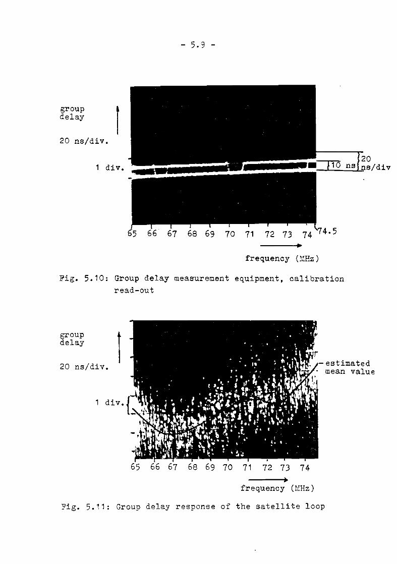
- 5.9 -

group Idelay

20 ns/div.

1 div.20

._"""-_---..1'-=08/d i v

frequency (MHz)

Fig. 5.10: Group delay measurement equipment, calibrationread-out

groupdelay

20 ns/div.

1

r. - estimated

. mean value

65 66 67 68 69 70 71 72 73 74

frequency O;~Hz)

~ig. 5.11: Group delay response of the satellite loop

- 5.10 -

5.4. Spectral measurements

To study the systems performance, several spectralmeasurements are made. The results are dicussed andcompared with the HPA/LNA loop results. All the measurementare made with the measurement set-up of figure 4.3 (set-upB) •

In figure 5.12 the round-trip earth -·satellitespectrum is shown when no signal is transmitted.The Eo-beacon transmitted from the satellite is clearlyvisible at- 79 r.lliz. Other distortions and interferencesdo not appear above the received noise band with a B

n(resolution bandwidth) of 30 kHz. In figure 5.13 tnereceiver spectrum is shown when a unmodulated carrieris transmitted and the satellite TWT is near saturation.In addition trr the looped-back 10 ~EHz sigDal and thereceived Bo beacon, a third component is visible at61 MHz. This component of the received signal is thethird-orde intermodulation product (2fc - f B ) of the

transmitted carrier and the Bo beacon. Due tg drivingthe satellite's T~ so near saturation, this

.".. +-

,---;--.

.....

+' --t

,~ ,

-+-

-r ' -+-

55 70 75 80 85 90 95•

(dBm) 20~

M

I-30Q)0]

\»r-la3s::a3 -408~M -50+:'0Q)

0.rn -60+:'a3

r-I -70Q)

>Q)

......M -804~··Q)

ii:00.

Fig. 5.12:frequency (MHz)

Round trip earth-station/satellite loop spectrumwhen no signal is transmitted (set-up B in figure 4.~

- 5.11 -

component is formed (see figure 5.3). Comparing figures5.12 and 5.13 makes it possible to ~etermine whicbdisturtances are ;robablj transmitted from the satellite,because the ';)ower level diminish when an extra unmodulatedcarrier transmitted by the ~JT stdtion, is transmitted.This is partly due to the fact that the maximum availableoutput power of the TWT must be shared by the various

(dEm)'""

9590

, '--t 'H--

, j-j-

" . H-

B mo ,

8580

70 MHz signal

I -+-r- ,'"

7570

, '"

++ i, ~ ....i·'~+- H·J /++/-i

"I-"--'-"

bO 65

, .... It

. h- +1 t

+-r~ H .

-+-i- ++

-20

-3oE 1ntermodulationt: product.~, .,"" ,.

-40 ' ~l: ::tL;:; :,~rt..::;:,;-=.:4 ;-,---:....,..,. 1+"'-' f---;-'--- '

,..... f , _. ..;"'+~ H

-50.h--'--

-70

frequency (MHz)

Fig. 5.13: Round-trip earth-station/satellite loop,w~en an unmodulated carrier is tr3ns~itted,

with set-up B of figure 4.3.

signals, and )artly due to the non linear transfercharacteristic of the satellite's TWT. Tbis causesextra intermodulation products which contain part ofthe total power. This is also valid for the noise bandwhich is suppressed by approximately 4 dB (limiter

- 5.12 -

effect (8]). Similar to the method described inparagraph 4.8, the G/No ratio was measured. Jith thespectrum analyser set 3.S described in paragraph 4.8,the instrument read-out was:

c ~ -9.4 dBm

N ( ) ~ -96.3 dBm/Hzo at 71 MHz

'!!his gives:

a III~ - 86.9 dBHz

o( 5-4)

This is approximately 0.9 dB better than the valuecalculated in paragraph 4.2 and could be explained bythe fact that the link budget calculation is set upfor weather conditions occurring during only 1% of theworst month of the year (see paragraph 4.4). This wasnot representative during the measurement conditions,Furthermore it might also be caused by c~ulative measurementerrors (including: actual transmitted power +/ - 0.2 dB,pointing loss +/- 0.2 dB, satellite's TW! output back-off +/- 0.2 dB· (see figure 5.3), system noise temperature+/- 0.2 dB (see figure 4.19).

In figure 5.14 the looped-back signal is shown in a 500 MHzspan (resolution bandwid~h of 100 kHz). Clearly visibleare the looped-back carrier at 70 MHz, the Eo beacon andthe intermodulation product of the two. All the otherdisturbances do not appear above the received noiseband.

In figure 5.15 the looped-back 4 Mbit/s indirectlymodulated signal is shown. The same is done, in figure 5.16,for the 4 Mbit/s directly modulated signal. In figure 5.17

(dBm)

1-10...

-20~Inter­IIlOdulationproduct-30 o •• - ,. ,

-40

-50

- 5.13 -

. r-

70 MHz signal

second harmonic

'~~0r--r::~~,~+;=

••~o~ •. .~+' o~_' ~ ° +~:=::..... ' ."-"'-~"- i~~

-70

-80

-90o 100

. ++

200 300

0_ L

400 500

frequency (MHz)Fig. 5.14: Looped-back spectrum, using the satellite loop

in a 500 MHz span (resolution bandwidth 100 kHz,with set-up B and resolution bandwidth 100 kHz)

the indirectly modulated 8.448 Mbit/s looped-back signalis shown, whereas the directly modulated 8.448 Mbit/slooped-back signal is shown in figure 5.18. o In all fourfigures the Bo beacon is clearly visible. 1he intermodulationproduct of the Bo beacon and the from the EUT transmittedsignal is not visible anymore. Because the transmittedsignal is now modulated and its ~op is laying about 20 dBlower than before (compare figures 5.13 and 5.15), theintermodulation product at 61 MHz is also modulated andits top is about 20 dB lower. However its correspondingpower will be the same (and it is still present).

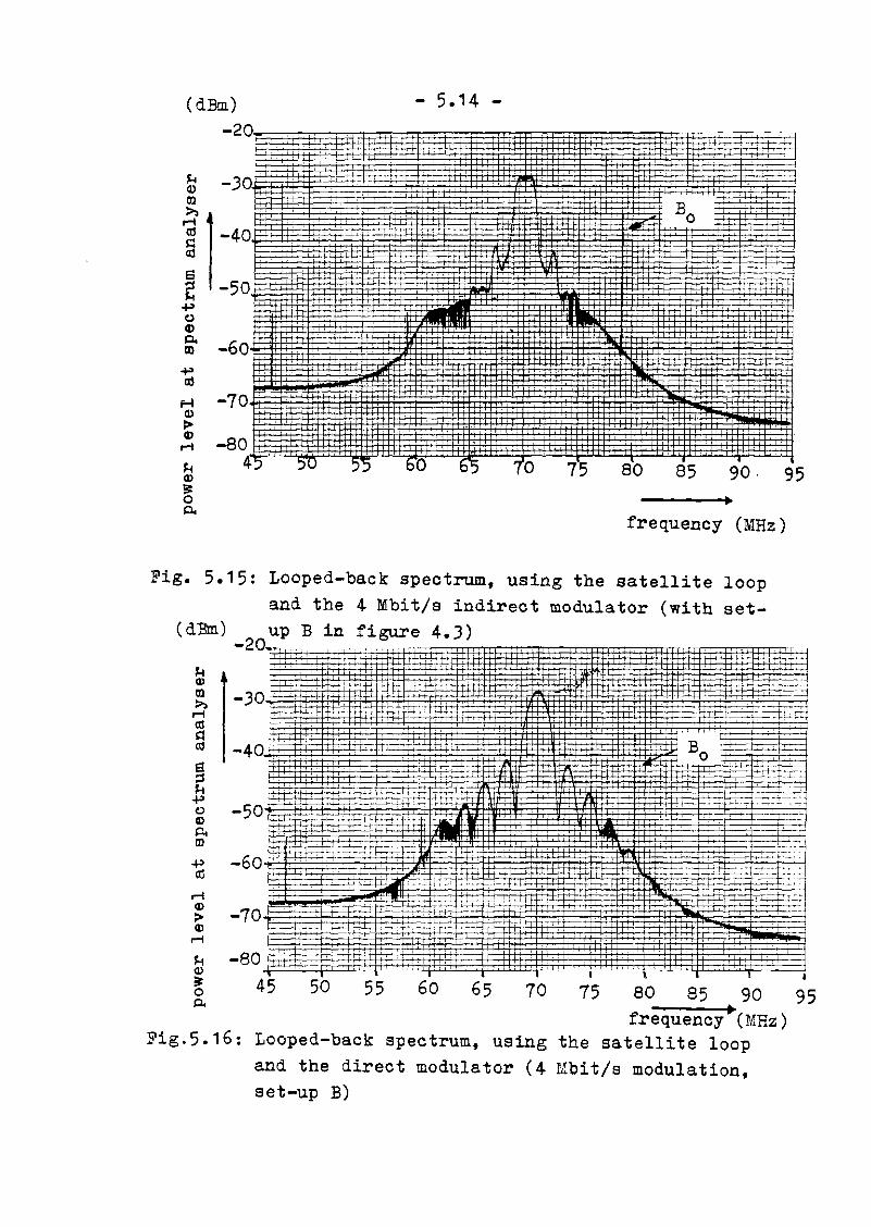
(dBm) - 5.14 -

~ -30!II

!1-40

~ -50+:>()4)Pom -60

~±~~~~-~-~

':J+T.-'-f-"""";";" H·+

'...,'+

•

H' .'~ ._,_c..~.· •

• '-4-

, , I, ~·"t-~-Y-4...,...,..~

frequency (MHz)

+:>as

H -70CD~4)

-80,....~

~'-"- .CD~0Po

bO 6 70 75 80 85 90· 95

Fig. 5.15: Looped-back spectrum, using the satellite loopand the 4 Mbit/s indirect modulator (with set-

(dBm) up B in figure 4.3),.

. t,

, -r+-+

-H-,

I I

75 80 85 90 95•frequency (MHz)

the satellite loopMbit/s modulation,

7065

, , ~

60

.,"t,~

, .HH-H. ,..... .

50 55

-30-

-40

-50

-70

~CD!II>,,....etls:letl

El:;j~~oCDAlD

~ro,....CD>4D,....~ -80Q)

~ 45A

Fig.5.16: Looped-back spectrum, usingand the direct modulator (4set-up B)

(dBm) - 5.15 -

90. 95

r-L- ... -~ . ----+-~ ~-

..;.........~+

'- :-=t:-- -

B "o ,

85807570

r+h--r

65

t-

60

-, ,-. - ri--+-'- -,H- '~~J 7--

-r- ~ j. •

..... r~;~:- ~++-t- +-H-~

55

ri-

, '

.~~..:-., .... +::~: h.-:~ ~,

50

~ -20 _ _...,...-+--r-...,....." e-: --;.I~-· ,.....+-f-+--L,-.-t-7'

~ ~.,."'h- --+,f·f-+'-::j:::-rr:-...:.:.:~~

~ r-30 -'s:: 'oj

ee -40 -,f--,--

~ ----l ~~.:.:. T::.:t.:---c'

~ <-' ';':};~T2:;:'? •~ -50~. ~~-=~~T ~T-,-. "L@jiltc;.

+ ~~""".-4+- ~""h- .1--_..-,.- II.~ ,

, ,r:;....;..·f-H-l- • c;~ f~ " .;...,..r'-H- ,-i. '- . " r,: r ,i+: ,++r"r t;;""; H-t

~

a3 ::::r-4 -60Q)

>Q)

r-4 -70~0)• -800A 45

frequency (MHz)

i"""""1

Fig. 5.17: Looped-back spectrum, using the satellite loopand the 8.448 Mbit/s indirect modulator (set-

(dBm) up B)-20 --! ,~,

i +...;._~ ... T~-' ~

+==

95•

90..

85

-',

8075706560, ~,

55

-60

-70

Fig. 5.18:frequency (MHz)

Looped-back spectrum, using the satellite loopand the direct modulator (8.448 Mbit/s modulation,set-up B)

- 5.16 -

It is interesting to compare the above mentioned resultswith the results of chapter 4. Of course the Bo beaconand its intermodulation products with the transmittedsignal are not present in the received spectra, usingthe local translator loop. The strongest difference isfound between the spectra of both loops when no carrieris transmitted (figures 4.8 and 5.12). Due to extrafiltering in the satellite and extra transponder noise(paragraph 2.1) their spectral noise density functions-at the output of the downconvertor differ. However figures4.9 and 5.1), which are more significant differ only verylittle and the measured C/No ratio's differ only 0.2 dB(paragraph 4.1 and (5-4)).

Comparing the direct and indirectly modulated 4 Mbit/ssignals 'for both loops a power level shift of approximately7 dB is visible. This corresponds to the fact that in themeasurement concerning the local translator loop, theinterfaci1ity link of )0 m coaxial cabel and the hybrid,with a total attenuation of approximately 7 dB, wereleft out.

Apart from the above mentioned differences only veryminor differences between the spectra of both loops occur.From this and the results of paragraph 5.5 it can beconcluded that the translator loop can be used tosimulate the systems performance, during the earth­satellite loop transmissions, very good.

5.5 BRR versus Eb/No curves

Measuring the BER versus Eb/No is one of the mostimportant measurements, because from this the actualsystem performance can be assessed.The method of measurement is already described in

- 5.17 -

paragraph 4.6 and will not be repeated here. The resultsare tabulated in table 5.1 and shown in figure 4.25. Dueto equipment failure the BER versus Eb/No curve of the4 Mbit/s indirect modulator and the direct modulatorwith 4 Mbit/s modulation could not be measured. Thiswill be done in future experiments.

Table 5.1: Satellite loop BER versus Eb/No8.448 Mbit/s

indirect direct

Eb/N"o Fe Eb/No Fe(dB) (dB)

17.8 4 10-b 16.7 1 10-0 .

17.2 6 10-6 16.5 1 10-6

16.7 1 10-5 16.3 2 10-6

16.2 2 10-5 15.4 9 10-6

15.6 3 10-5 14.8 1.4 10-5

15.4 3.5 10-5 14.4 3.5 10-5

14.8 5 10-5 14.0 9 10-5

14.4 8 10-5 13.5 3 10-4

1"4.0 1 10-4 12.8 7 10-4

13.5 2 10-4 12..2 9 10-4

12.4 4 10-4 11.5 1.5 10-3

12.6 4 10-4

11.9 7 10-4

11 1 2 10-3

In table 5.2 the degradation due to distortions &interferences is given. (see figure 4.25)

Table 5.2: Degradation due to distortions & interferences,t 11 t 1us~ng the sa e i e oop

modem deQTsdation8.448 Mbit/s indirect 1.'5 dB

- 5.18 -

The degradation due to distortions & interferences andimplementation losses of the direct and indirect 8.448Mbit/s modem are given in table 4.13 in chapter 4.Again this can probably be reduced by approximately 0.8 dBif the extra degradation, due to improper functioning ofthe 8.448 Mbit/s demodulator as described in chapter 4.

From figure 4.25 the extra degradation of the satelliteloop compared to the translator loop can be determined~

For the direct modulator it is found that the extradegradation of the satellite loop varies from 1.2 dB atFe = 4.10-4 to 0.6 dB at Fe = 10-6• For the indirectmodulator the extra degradation varies from 0 dB at

-4 . . -6Fe = 2.10 to 0.9 dB at Fe = 4.10 •

Apart from the extra degradation, when the satellite loopis used, the HPA/LNA gives a good simulation about thesystem behaviour during satellite transmissions.

This extra degradation is probably due to distortion bythe present Bo beacon and the intermodulation product ofthe Bo beacon and the signal, group-delay variation andthe satellites filter and local oscillator.

It would therefore be interesting to measure the group­delay response more accurately, the satellites (input)filter characteristic and the phase noise contributionof the satellite.

- 6.1 -

6 Conclusions and Re~ommendat1ons

The following conclusions and recommendations areoffered witb respect ~o the work presented here.

6.1 Conclusions

a) An updated survey has been given of. the digitaltransmission system used by the TelecommunicationD1.vision of tbe EUT for experiments via the OTSsatellite.

b) The dynami.c range, of a carrier tracking loop fordepolarization measurements, is calculated forvarious levels of up-plus downlink fading.

c) An accurate calculation of phase jitter, for a

wide range of loop-bandw1dths and with arbitraryphase noise spectral density, has been perfor.med.

d) An analytical determination of the optimumbandwidth of PLL loops, applicable to bothsynchronous digital demodulation and propagationbeacon tracking loops, has been4ezoived.

e) A procedure for calculation of the optimum loopbandwidth and the resulting phase jitter degradationfor differen~ levels of up-plus downlink fading levelsis given.

f) Several systems for compensation of depolarizationeffects in both singular and multiple uplinksatellite systems has been rev~ewed. Such systemsare especially important for frequency reuse.

- 6.2. -

g) The existing link budget calculation is improvedwith data measured during the satellite loopexperiments, such as the satellite ~WT outputback-off (1.7 dB) andthe:amount of dis~ortion

and interference degradat.ion (1.5 dB).

h) It is shown that there is practically no adjacentsatellite channel interference (for 4 Mbit/smodulation) in the A-transponder band of the OTS ,and that the narrowband filtering after the ear1:hstation TWT" can therefore be replaced by morebroadband filtering.

i) The single sideband noisa f.igure of the stationsreceiver has been measured and optimized (5.2 dB).

j) The frequency stability and phase noise spectra o~

the various oscillators have been measured.Furthermore, the overall phase noise contributionis measured and evaluated. The total amoua~ ofphase jitter for the current impJementation iscalculated (4.3 0

) and witb this the minimumobtainable probability of error is derived (2.3 10-8 )

k) For low bitrates (such as 64 kbit/s for sope traffic),which require less tz!anamission power, the loopbandwidth reduces and the phase jitter increases.Due to poor phase noise performance of both thepresent upconvertor and local oscillator in the

. data receivez; the phase noise degradation is likelyto be severe.

1) The modem implementation losses have been measuredand are found to be much larger (3.5 dB (minimum)instead of 2.5 dB) 'than previously estimated.

- 6.3 -

m) Ampl1~ude and group-delay responses of the entire .system have been measured. The group-delay responsemeasurement is rather noisy, probably due to poorphase noise performance of the entire system andthe inability to adjust the loop-bandwidth ofthe measuremen~ equipment.

n) Spectra of the received signals at 70 ~!Hz and BERversus Eb/No curves of both translator and sateliiteloop have been measured.A demonstration of this system has been given.

0) It is found that- the direct modulator is slightlybetter than the indirect modulators used (therequired Eb/N

Ois reduced by nearly O~5 dB when

using the direct modulator at 4 Mbit/s)

p) The translator loop s~ulates the s.tel11te loopbehaviour well. The extra required Eb/No for the, sa'tellite loop is less than 1 dB.

q) Although there are still points for improvementand more permanent solutions~ the exp~~imental

sys~em works and can be used for 8.448 Mbit/s~ideo transmissions.

6.2 Recommendations

a) In view of conclusion h) (paragraph 6.1), it isrecommended to replace the narrowband filter afterthe earth-station TWT by an - already aVailable ­broadband filter in order to increase thetransmitted power (bij approximately 0.5 dB [1] ).Since the uplink CINo ratio is smaller than the

downlink CINo ratio, the overall CINo ratio couldbe increased significantly.

- 6.4-

b) In'new-of canc:lusions j) and k), it is recommendedto improve the phase noise characteristics ofboth upconvertor and local oscillator, especiallyif satellite experiments with lower bitratesare t'o be carried out.

c) The modem implementat'1on .10sses, .are, found "to' bemuch larger than expected (concluaion 1», and ­should: be improved upon.

d) It would be interesting to investigate whethera steeper 1F filter in the receiver would reducethe inflnence of the Bo beacon and o~ inter.modula~ion

products and so improve the total system performance.

e) It is recommended (see conclusion m» to repeatthe group-delay measurement-,. either when the phasenoise performuance of the link has beenimproved, or with different and more sui~able

measuring equipment.

- 7.1 -

7 REFERENCES

[1] L.J.C. Vers~eegb. Microgolf-communicatiekanaalvia de "Orbital ~est. Satellite" (OTS) •••S~ thesis,Eindhoven University of ~echnology, department ofelectrical engineering, Telecommunications Division.August 1982.

[2) Response to INTELS~~ RFP-238, Technical andManagemen~ Proposal, Par~ I, Eindhoven Universityof ~echnology Netherlands, April 1982.

Dl J.Th.R. Schreuder, Satellietcommunicatie-Overzich~

van enkele recente ontwikkelingen, RUimtevaar~,

De-o embe:e- 1982.

~] P.J. Bartholome, Propagation Experiments at11/14 GHz as Part of the European Communica'tionsSatellite Program, Proc. IEEE, vol. 65, no. 3, March 1977.

~J J.M.G.A. Ouderling, Ontvangsystemen voor propagatie­metingen met behulp van phase locked loops, M.Sc.thesis, EUT department of EE, March 1978.

~J CCIR, 1982, "Propagation data required for spacetelecommunication systems", vol. 5.

[7] C. J. Wolejsza, "Effects of oscillator phase noiseon PSK demodulation", Comsat technical review,vol. 6, no 1, spring 1976.

[~ F. Gardner, Phase Lock Techniques, New York:John Wiley, 1966.

.....~] W.C. Lindsey, M.K. Simon, Carrier Synchronization

and Detection of Polyphase Signals, IEEE Trans.Comm. Tech., June 1972: pp. 441-454.

- 7.2 -

Bo] J.J. Spilker, Digital Communications by Sa."ellite,Prentice-Hall, Inc., Englewood Cliffs, New Jersey,

1977.

~1] T.S. Chu, "Restoring the orthogonality of TwoPolarizations in Radio Communication Systems,I," B.S.T.J., 50, no. 9 (November 1971),pp. 3063-3069.

021 G.A~S.H. Schijndel, Verwerting van propagatiemeetgegevens a!komstig van een 11 ~ Satel11e~­

verbinding me~ de O~S, M.Sc thesis, EindhovenUniversity of Technology, department of electricalengineering, Telecommunication Division, KErch

1983.

~3] V.H. Rumsey, G,.A. Desohamps, M.L.. Kales andJ.I. Bohnert, ~echn1ques for Handling EllipticallyPolarized Waves with Special Reference ~o Antennas,r.R.E. Proc, May 1951, pp. 533-552.

~4] D.P. DifonzQ,W.S. '1rachtman, A.E. Williams,"Adoljtptive polarization control for satellitefrequency reuse systems", Comsat technical review,vol. 6, 1976, pp. 253-283.

~ 5] S.K. Barton, "Methods of adaptive cancellationfor dual polarization satellite systems~, Themarconi review, vol. 39, no 200, First- Quarter1976, pp. 1-21.

~6] Lin-shan-Lee, "A Polarization Control System forSatellite Communications with Multiple Uplinks",IEEE Trans. on Communications, vol. COM-2Ji, no. 8,

August 1978, pp 1201-1211.

- 7.3 -

~7J M. Nouri, M.R. Braine, "An adaptive interferencecontrol system for earth-satellite links above10 GHz", The marcon! review,- vol. 43, First. Quarter1980, pp. 14-28.

[18] ESRO-CERS, "Communication Satellites Programme,The Orbital Test Satellite", Data Book, issue'l!wo, EC/4664/PB/sa (Rev. 1), March 1975, ESTEC.

~9] B.C. de RBg~, "Vier-fasen-modem van een sat.elliet­communieatiekanaal voor twee da~asignalen van

2 Mb",M.Sc. thesis, Eindhoven University of ~echnology,

department of electrical engineering,Telecommunication division, July 1978.

~O] J.Th. Nagelhou~, Een 8,448 Mbit/s modem voorbeeldtelefonie~experimentenvia communicatie­satellieten, M.Sc. thesis, Eindhoven Universityof TechnQlo8Y, department of electricalengineering, Telecommunication Di~ision, March1983.

[21] ESA, Report on In-Orbit Measurements OTS, ESA/JCB/(80)1, vol.l: Principal Classical Repeater Tests., 12december 1979.

[22] ESA, Report on In-Orbit Measurements OTS, ESA/JCB/(80)1, vol. 2: Antenna and Propagation Tests., January1980.

[23] J.D. Kraus, Radio Astronomy with a chapter onradio-telescope receivers, MeGrown-- Hill 1966.

[24] J. Swijghuisen-Reigersberg, Private Document.ation,Eindhoven University of Technology, department.of Electrical Engineering, TelecommunicationDivision.

- 7.4 -

~5] Hewlett Packard, Technical Data Spectrum Analyses.model 8566A, September 1979.

ji6] Hewlett Packard~ Understanding and measuringPhase Noise in the frequency domain, applicationnote 207, October 1976.

[27] V. Bhargava, e.a., Digital Communications by~atellite, A. Wiley-Interscience, New York, 1981.

[28] A.B. cralson, Communication Systems, second edition,T"okyo: McGraw-Hill Kogakusha, 19"';.

~9J ESA, Report on In -Orbit- Measurements OTS,ESA/JCB/(80) 1 , vol. 3. other Payload Tests, March1980.

Do] E.J .... Wijdemans, Private documentation,Eindhoven University of Technology, departmentof Electrical Engineering, TelecommunicationDivision.

D1] RFP INTELSA~-2J8, dated 26 February 1982.

- 8.1 -

8 GLOSSARY OF NOTATION

Symbol

A1,2

B

Be4

BERBlFBL~opt

~1,2,3

~, BPSK

B0,Ox,20,21CC (1),(2)

polCQPSK

Cup, downCW

Co

C1,2,3,4

C1 1,12,13,14DCQPSKDSBEbE(c)c

EHFEIRP

EUT

Definition

axial ratio of ellipsesI and II

bisectorbandlimitation of cons~ant

04bit-error-ratebandwidth of IF filternoise bandwidth of PLL-loopoptimum BLsolutions of equation todetermine BLoptequivalent noise bandwidthBinary Phase Shift KeyingBeacon notationsCarrier powerCo-polar field componentrrcrheren~ Quadri Phase Shif~

KeyingConstantsContinuous WaveNominal Carrier power (whenattenuation equals unity)Constants in Phase noisespectrumConstants

Differential Coherent QPSKDouble Side Bandbit Energy(counter)clockwise polarizedfield componentextra high frequencyEqUivalent IsotropicallyRadiated Power

Eindhoven University ofTechnologyx and y field components

first usedon page

3.62.20

4.192.20

2.192.322.31

2.52.27

4 A/4 .12 .72.7/2.104 .35

2 .52.22 .16

2.18

4,.31

4 ..354.252.273,;J

4.72.11

1 .1

3 .3

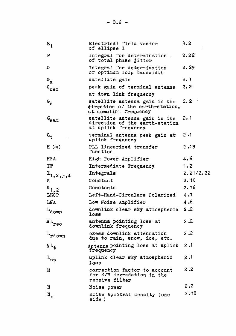
G

G tsa .

HPAIPI 1,2,3,4K

K1 2,LRCPLNALdown

M

- 8.2 -

Electrical field vectorof ellipse IIntegral for determinationof total phase jitterIntegral for determinationof optimum loop bandwidthsatellite gainpeak gain of terminal antennaat down link frequencysatellite antenna gain in the«irection of the earth-station,a~ downlink frequencysatellite antenna gain in thedirection of the earth-stationat uplink frequencyterminal antenna peak gain at:uplink frequencyPLL linearized transferfunctionHigh Power AmplifierIntermediate FrequencyIntegralaConstantConstantsLeft-Rand-Circulars PolarizedLow Noise Amplifierdownlink clear sk,J atmosphericlossantenna pointing loss atdownlink frequencyexeS8 downlink attennationdue to rain, snow, ice, etc.Antenna pointing 10s8 at uplinkfrequencyuplink clear sky atmosphericlosscorrection factor to accountfor SiN degradation in thereceive filterNoise powernoise spectral density (oneside)

3.2

2.22

2,.29

2. 1

2.2

2.2 .

2. 1

2 .18

4.61.22. 21/2.22

2. 16

2. 16

4.14.62.2

2.2

2 .2

2.1

2.22.16

0C

OD

OMT'OTSP1ti

P~cSJ

P [~/no cSJ

PLLPrecPsatPSKPtPTI

QPSKR

- 8.3 -

minor axis of polarizationellipse Imajor axis of polarizationellipse IOrtho Mode TransiucerOrbital Test Satellitey to Xfield component ratioof elljp,se 1 t ierror rate during ou~-of-lock

conditionerror rate during lockconditionlumber of bits during cycleskip divided by total numberof bitstotal number of bits lessnumber of bits during cycleskip divided total number ofbitscombined probability oftransmission errorprobability of errorcontribt*ed by cycle skippingprobability of error due tothermal noisePhase-Locked-Loopearth-station received powersatellite received powerPhase-Shift-Keyinguplink transmitted powerPhilips TelecommunicationIndustriesQ-function for calculationof BER with coherent detetionQuadri-Phase-Shift-Keyingdistance between earth-stationand satellitebitrateRight-Hand-Circular-PolarizedSignal powerSignal to noise ratio ofbeacon signal

3.2

3.2

3.91. 1

3.4

2-28

- 2.28

2.28

2 .1

2.2

2.1

2.1

2.1

4.6

2.26

4.12.2

2 .11

- 8.4 -

2.16

single channel per carriersignal to noise ratio in PLL­loopSingle Side BandShort Slot HybridPhase· noise spectrumPhase noise spectrum ofLocal Oscillator earth-s~ation

Phase noise spectrum at output- 2-.16of earth-station receiverPhase noise spectrum ofsatellite translator oscillatorPhase noise spectrum transmitted 2.16from earth-stationPhase noise spectrum at output 2.16of earth-station receiver whenthe rain attenuation equalsunityaverage atmosphere temperaturemeantime to unlock for secondorder PLL~elemetry beaconnoise temperature indicatedby rain absorptionearth-station receiver noisetemperaturesatelli~ receiver noisetemperature refered to thesatellite receivertotal system noise temperature 2 4refered to earth-station receiver •total system noise temperature 2.4refered to earth-stationreceiver when an out-of-­transponderband beacon isreceived

Tr4 TIl­xtttrain

'l!rec

'l!absT:av _

-SCPC

(SiN) L

SSBSSH

16(0/)-S (w}fr, LOS (t:Q)

"recS «/?).

c1-,-ss'tS (c.v}f,up

S (ee)o

T'UL

~transponder contribution to total system 2.4nois~ temperature from thesatellite transponder referedto the earth-station receiver

lQSan time during which PLL-Ioop 2.25remains unlocked

TWT

USBTraveling Wave TubeUpper Side Band

X

XPDxprx (1),(2)

polX1 ,2

y

cf

k

Akk (~)

la1

AupAdownJ!

- 8.5 -

X"'axiscross-polar-discriminationcross-polar-isolationcross-polar field componentsdirection of major axes ofpolarization ellipsesY-axis

Hc4/B:Lf'r~quency

Boltzmannts constantdifferential attennationleft-hand side of equation(2-64)variable attennationroot-mean-square

constantscounter clockwise rotation ofmajor axis of polarizationellipses I and II relative to thepositive X-axisantenna main beacon factorangle of introduction ofdifferential attennation relativeto positive X-axis(one side) spectral moise densityangle be~een major axis of twopolarization ellipsesuplink wavelengthdownlink' vmvel-ength~'correction factor"to ae-conn-t forthe loss in S/Hr&t±odu'~ Vofrequency doubling or remodulationin carrie~ recovery loopangle of introducitio.Q ofdifferential phase-shi~ relativeto positive X-axis

damping factorrms phase noise within theangu-lar bandwid th (W1- "2)rms thermal noise contributionto the total phase jitter

3.22.72.72.73.2

3.22.-234.30 .2.,53.102.31

2.3 1

3.2

2.43.,10

2,.7.3.1

2-.18

2.25

2.19)·.13

3.53.5-

<r¢'L

lT~~

"'t" P .

q1 2!:. 4'

?f)(w

- 8.6 -

rms phase jitter in carrierrecovery looprms total phase jitter

~iable phase shiftdifferent~al phase shiftangle between two linea1rpolarization vectorsangle between :a and_posi1iive X-axis 3.~

angular frequency 2.16natural frequency of a 2.Z5linear transfer function

arg (.) angle between vee-tor and 3 .. 4positive X-axis

~ approximately equal to 2 .. 11A which is equivalent to 2.11=~ is defined as 2.3-E vector notation 3.2I • I modulus 2.7

~ convolution 2.16

- A.1 -

APPENDIX A: Integral calculations for phase jitterdetermination

A.1. Calculation of I 1

The first integral of equation (2-28) in paragraph 2.2is calculated:

where c.u ~ ° (A-1)

2~~ _arctan 2"'1;JT'2 't

P p

2substituting z =w gives:",,2-

~ 2

J~C1 dz C1fp 22z

I 1 ~ 2 4 = c. .arctan~Z +---r (,. '0 2

~"t~ P ,p

= ~.{arctan

taking, w, -+ ° and ~ --f>00 givee:

(A-2)

2C"'p {7\ 1I, = 4 · ~ - o} (A-))

with Tp =~ gives:

9C,'7\I ­

1 - '28~~(A-4)

where w ~ 0 (A-S")

- A.2 -

A.2. Calculation of 13

The third integral of equation (2-28) is calculated:

w2 w2

JC w3dw J.k dw

4I

- 3 _...:....4-,...3 ___3- 4 4 - -4 4

w w +::-4 w w +---r, T 1 T""

P P

substituting z =w4 gives:(.04

2 ,

I 3 =! tc3 d~ = te3. 1n{Z(.l,)4 z +~

, " 'I-P

+ 4}?p

w4.2.

w4,(A.-6)

--I co; co, ~ 2XBnrtaking w, -+ 0 and (.02 -+00 and knowing C3 w, > 27fBIF

(A-7)

leaving out the accent and with 'p = ~ gives:

, [J 4 '024~4

} {'024BL4!]

13 = tc3 In (2ABIF ) + 81 - Inl 81 =

1 f 1.296 4Bu41lC3.In , + 4 (A-8)'024BL

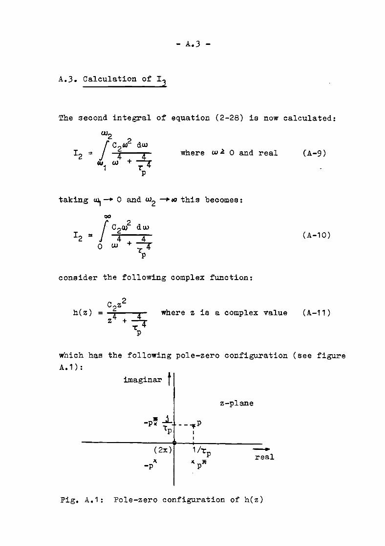
- A.3 -

A.3. Calculation of I 3

The second integral of equation (2-28) is now calculated:

where w ~ 0 and real (A-9)

taking ~ -+ 0 and w2 ~oo this becomes:

consider the following complex function:

(A-10)

h(z) where z is a complex value (A-11)

which has the following pole-zero configuration (see figureA.1):

imaginar fz-plane

_p~ .l... - -~pLp I

I

(2x) 1/"t'p --.real

~ ~ pJe-p

Fig. A.1: Pole-zero configuration of h(z)

- A.4 -

Furthermore one can write:

substituting y = jw gives:

(A-12)

which is equal to:

where y is imaginar

(A-13 )

Consider the following contour C (figure A.2):

jR...-_

Tz-plane

Fig. A.2: Integral contour for calculation o£ 12

- A.5 -

From complex function theory one gets:

! h(z)

R 0

dz = I hew) dw + !h(Z) dz + I hey) dy =C 0 jR

T2~j Res{h(p)J (A-14)

where:Res{h(p)J ~ residue of h(z) in p

From complex function theory one gets:

Res ih(p)J = lim h(z).(z - p) = limz~p z-p

C z22lim -~-~~--~-~=

z-p (z2 + j~) (z + 1.'; j)T PP

2C (1 +..,i)

2 ~G C2 7

___--,:~.........r;P:....-----= P

[2] 4(1 + J')(1 + j) + 2j .2. 1 + j

"t' 2 'pp

(A-15 )

for R~ 00

(A-16)

From (A-14), (A-15) and (A-16) one gets:

- A.6 -

00

f hew)

o

o

dw + Jh (y) dy =joo

(A-17)

Together with (A-10) and (A-13) this becomes:

and with Tp :: k this equals:

2T Jo C 31\ 2.~

I - -----,~-2 - 4(1 + j)2 -

A.4. C"alculat1on of T4

(A-18)

(A-19)

The fourth integral 14 of equation (2-28) is calculatedsimilar to the previous one.

consider:

',vith w1 -+ 0 and w2~ C() and knowing that c4

one gets:

(A-20)

={:~W~2 Bc4c.u>2 Be

4(A-21)

- A.7 -

2XBC at 4

J 4 4-:rtP d- 4 4 w

o (JJ +::-4Tp

(A-22)

leaving ou~ the accents gives:

(A-23)

with \ =~ and substituting x =

this becomes: 1

2ifB • [4 fI' ~1C4 j J

_4~c4~ J .' dxj x4 + ,o

(A-24)

or:

(A-25)

BDefining: 3~ 04

2fi·~

J ~F(Br) = ;rr.: dx

o x4 + ,(A-26)

(A-27)

- A.8 -

BCConsider F(~); for ~ -+~ one gets:

FCO)

define:

(A-28)

f(z,) where z is a complex value (A-29)

which has the following pole-zero configuration (seefigure A. 3) :

imaginar tz-plane

li .at - - "'fq_q xfl I

I

1/{Z reat-q x l<q]f

Fig. A.3: Pole-zero configuration of fez)

Furthermore one can write:

FCO)= J" ~ d.x - 1 JOO~ d(jx)

o x4- + 1 - J 0 ( j x) 4 + 1

00

= _j!~ d(jx)

o (jx}4 + 1

(A-30)

- A.9 -

substituting y = jx gives:

F(O)j!~ 2/2 dy

. 1:__= -J

o? + 1 = J

o 212 dy. 7rJ ~4--

jco Y + 1(A-31 )

which is equal to:

-jF.'CO) (A-)2)

Consider the following contour C (figure A.4):

1/ 2

z-plane

x x

Fig. A.4: Integral contour C for calculation of F(O)

From complex function theory one gets:

I fez)a

R

dz =Jf(x)o

dx + I fez) dz +

T

oJfey) dy =

jR

2Xj Res f(q) (A-33)

- A.10 -

Again one gets:

Res {f ( q )1 = 1 im f ( z ) • (z - q)z..q

28. 2fi1im 7t _ __-.;.;,7\" =Z q (z~ + j)(z + 1 + j) - (2j)JZ(1 + j)

IZ1X

j - 1

j'9Taking z = R.e one gets:

~

/ f~ 2/Z. jRe jlf

f ( z) dz = ::i j 4~ dCf ... 0ORe + 1

T

(A-)4)

for a... oo (A-)5)

From (A-))), (A-)4) and (A-)5) one gets:

co

I f(x) d.x +o

o

I fey) dy =

joo

(A-)6)

Together with (A-28) and (A-)2) this becomes:

(1 - j)F(O)

or:

F( 0) = 1

(A-)7)

(A-)8)

For tL = B one gets:-.L C4

F(BC )4

- A.11 -

(A-39 )

Calculating this integral with Simpson's (continuous)approximation rule and a ~exas Instruments T1 58calculator gives:

F(BC ) ~ 0.992 (A-40)4

Because fez) is a positive function and with (A-38) and(A-40) one' ohtains:

for (A-41)

Values of F(Br) when BL > BC4

are given in table 2.8 ofparagra.ph 2.3.

,A.5. Calculation of Ii

To determine the optimum loop bandwidth (paragraph 2.3)the derivative of (2-47) had to be determined•.From(A-4), (A-8) and (A-19) one can see that determiningthe derivative of the first three integrals, 11 through13, is not difficult. However the der~vative of the fourthintegral 14 cannot easily be calculated and will bedetermined here.

To this end the derivative of (A-2) is determined:

- A.12 -

2XBC

t =~ J 4C4W

4 dw(A-42)14 4 + 4L 0 w T4

P

which is equal to:2~B

~C4 4•= ~! C: ~4 (A-43)14

dW

04+w 34

or:

dw

dividing numerator and denominator by

(A-44)

[4 f2'.3· Brt1

8

- j gives:

substituting:x: = W gives:

(4~.~)

(A-45 )

- A.13 -

1

Defining:

one gets:

I 2KC414 : - J .G

B.2!. C42f2·~

dx = _ 2 lC3C4 •J B;:.X\ dx

o (x4 + 1)

(A-46)

(A-47)

(A-48)

BeConsider G(~); for ~ -co one gets:

G(O) =

Define:

(A-49)

al2. z4g(z) = 4 2 where z is a complex value (A-50)

(z4 + 1)

which has the following pole-zero configuration (seefigure A. 5) :

- A.14 -

imaginar tz-plane

_rlE r(2x'JC ~ -"1 (2x)

I

(4x) 1/12' --+real

J( )( :IE-r(2x) (2x)r

Fig. A.5: Pole-zero configuration of g(z)

Furthermore one can write:

G(O)

co

I 8"2' (j )41 zr· x

= J - .....------"'12:0- d (jz) (A-51)o (jx)4 + 1

substituting y = jx gives:

GeO) = -jj/O(J 8'!-y4

-....,;";",,,-~2 dyo (y4 + 1)

(A-52)

which is equal to:

/

0 812.y4d 2 dy = -jG(O)

joo (y4 + 1)

Considering the following contour C (figure A.6):

(A-53 )

- A.15 -

z-plane

T

1/

x (2% J

jR"---

ix '~2 --~r

(2%)'~ 1(2%)I

(4%)(2% ye

Fig. A.6: Integral contour C for calculation of G(O)

From complex function theory one gets:

/ g(z) dz

C

R

=! g(x)o

dx+

o

dz + I g(y)

jR

dy =

21\j Res {g(r)} (A-54)

From complex function theory one also gets:

{8/2' 4 I1 . d --,.r""zr__·_z ~z: a:z 2 2 1; 2

(z + j) .(z + + Yo)2

(A-55)

- A.16 -

1 • (2 j ) 2 fi( 1+j~1+ j )} 2:+1 •*2j ) 22 JZ( 1+ j )] :

(2j) {VZ( 1+j >}

8VZ.32VZ(1+j)-16VZ(1+j)-8JZ(1+U = -(1 + j)K _162 2X

(A-56)

j'fTaking z = R.e one gets:

/ f~ 8:'.R4ej4't.Rjejltg( z) dz = 4 j 4Cf 4 d~ - 0 for R ...... 00

o (R e + 1) (A-57)T'

From (A-54), (A-56) and (A-57) one gets:

o

! g(x) dx +! g(y) dy = 27rj-1 (~: tLo jco

Together with (A-49) and (A-53) this becomes:

(A-58)

- A.17 -

(1 - j)G(O) = 2~j.-(12; j)

or:

G(O) = 1

For ~ = Be one gets:43~

21Z 812 4

GCHC

) = I ~.x 2 dx

4 0 (x4 + 1)

(A-59)

(A-60)

(A-61 )

Calculating this integral with Simpson's (continuous)approximation rule and a ~exas Instruments ~I 58 gives:

G( BC ) ::! 0.9684

(A-62)

Because g(z) is a positive function and with (A-60) andCA-62) one obtains:

0.96 < G(Br) ~ 1 for (A-63)

Values of G(B:r) when ~ > He are given in table 2.8 of4paragraph 2. J.

- B.1 -

APPENDIX B: Microwave waveguide filters

Two filters, recently developed and placed in the system,are described in this appendix.

The two filters are:

- P-band waveguide filter in the 14 GHZ band, placed inthe upconvertor and directly before the direct QPSK .modulator, to suppres unwanted signal components.

- M-band waveguide filter in the 11 GHZ band, placeddirectly after the LNA in the data receiver. This isthe so called image rejection filter •. Its placement ismotivated in ~] and i~ reduces the system noisetemperature (paragraph 4.4).

Both filters were measured with the measurement set-upof figure B.1.

An air line is used, to be able to adjust the phase­reference-plane. The 10 dB attenuator is recommended bythe manufacturer of the network analyser.

After every measurement the filter was replaced by awaveguide of equal length and which was used as a reference.

To design the filters the program CFILTER, present at the~, was used. After specifing the filter, this programgives a design of the filter and calculates its amplitudeand phase response and return loss. One can chose betweena Butterworth or Chebyshev fil t.er. The Chebyshev filterswere chosen, because they are wider than the Butterworthfilters. The filters are of the direct-coupled-cavitiestype. For both filters, the program was runned severaltimes with different input data. The most suitable filterswere chosen.

B.2

HP 869~ A Sw~EP OSCI~LATOR 8TflP 9694 A ET 14--: 1 I ~H-P-8-69-5"'-A--:E-:T~1~39~8:----'1Unit 9.J - 12.4 GHz. Unit 12.4 - 18.J GHz.

N1==

Ii~

I Cv.SI-\A

?: P1:ba nd

~ I v cm P-band golfpijp

P-band circulator

Ov.

av.APC-7

N

ET •

1,; ....~ 12.4 - 18.:> GHz.P-band -

~lectronic counter~

I,II

- - - --I-

ET

Ov.

SMA

Circulator

SMA

I N-~------

,- .... ..., RADIAL COUPLER

7 - 12.5 GHz

I

L080

Automatic Frequency convertorHP 5355 A ET 1851

26,5 GHz Freq. convertor headHP 5356 B ET 1852

1~ dB EC.... -r-

NF-

N. av.

I SMA

-;:: ~ =6~ cm.

SMA .I av.I N

F

HP 5345 A ET 1850

ET 18J~

ET 18J6ET 18~9

HP 841:> B

HP 8412 AHP 8743 A

Network Analyser 2 - 18 GHz.Phase-magnitude DisplayReflection-Transmission Test Unitl2.J - 12.4 GHz + option ·~18 (18 GHz.)

ET 147J HP Mos~ley 7JJ5 B X-Y-recorder I:IP 8743 A

lJNKiiOI;lNReflection-Transmission Test UnitET 18::>~ TRANSMISSION RETURN

1==----I APC-7 J' EC 1831 BU SMA-male P or M;-L. -band

1= APC-7

APC-7AIR LINEECC 1816

1:> CMB

._ p:'PC=7_ F==

AFC-7ATTENUATOR

1::> dBET 18~3

G~C--7- F= I

EC 1831 ~ ,SMA-female

FILTER 1 J CM

'""-- ~ SMA = 2::> CMTransmission measurement ~================~

Fig. B.1: Measurement set-up to adjust and measure bothM-band 3nd P-band filter [1].

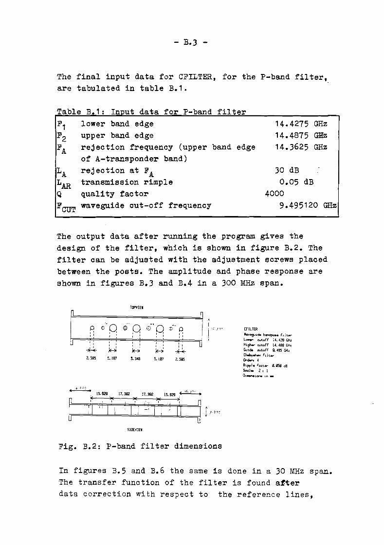
- B.3 -

The final input data for CFILTER, for the P-band filter,are tabulated in table B.1.

Table B.1: Innut data for P-band filterF1 lower band edgeF2 upper band edgeFA rejection frequency (upper band edge

of A-transponder band)rejection at FAtransmission rimplequality factorwaveguide cut-off frequency

14.4275 GHz

14.4875 GHz

14.3625 GHz

30 dB

0.05 dB

40009.495120 GHz

The outpu~ data after running the program gives thedesign of the filter, which is shown in figure B.2. Thefilter can be adjusted with the adjustment screws placedbetween the posts. The amplitude and phase response areshown in figures B.3 and B.4 in a 300 MHz span.

n

J

TlPVIEW

r", q >"

0"'0 M,

J " ? 3"0 <D q) 0 iD 0 CfILTER, I I I I I W""~id. b<r>dpae. fdt.rI I I : I

,I I I I

~ Lo... cutoff 14.428 GIIzI I

I I I I U Higl-- cutoffI I I I II I I I 14.488 GHz

I I I ' I I

~ I' GYid. cutoff 9. 495 GHz** H H **2.595 5. 197 5. 346 5. 197Chebyehe. f d tor

2.595 Order, 4Ripple Factor ~lI5B dBSeal .. 2 : 1Oi..".lone 1M _

,/;I 4 1 '1

.4 - -. 15.629 17.392 17.392 15.629.e ,6. P" ,

~.~~)I()i .. .' .;'.. I I I

( , ~ ~J ~ .fIll- &~o

SIOEVIEW

Fig. B.2: P-band filter dimensions

In figures B.5 and B.6 the same is done in a 30 MHz span.The transfer function of the filter is found a~ter

data correction with respect to the reference lines,

- B.4 -

which were obtained by replacing the filter by a P-band.waveguide of the· same length (see figure B.T). The filterW2S adjusted for minimum attenuation in a 20 MHz band aroundthe uplink centre frequency of the B-tr3nsponderband(14.4575 GHz).From figure B.7 one can obtain thay the actu~l measuredfilter characteristic is much wider than calculated (abouttwice as wide) and its centre frequency lays about 30 W~z

lower than calculated. However., the unwanted signals, outof the upconvertor, were suppressed and the filter couldbe used. The attenuation is approximately 0.9 dB (figureB.5) in a 10 MHz span around 14.4575 GHz. The phasecharacteristics is approxim2tely linear in this band (seefigure B.6 ),therefore the group-delay will be approximatelythe same for all frequencies within this band.

M b d filtt d t fT b' B 2a ... e • : l.npu a a or - an er. variable value

F1 lower band edge 11.765 GHzF2 upper band edge 11.825 GHz

FA rejection frequency (band edge of 11 .925 GHz20 MHz around image frequency)

LA rejection at FA 20 dB

L.l\R transmission rimple 0.05 dB

Q quality factor 4000FCUT waveguide cut-off frequency 7.889941 GHz

The output data of the program gives the desired filter,which is shown in figure B.8. The amplitude and phaseresponse are shown in figures B.9 through B.12. 'llietransfer function after data correction is foUnd infigure B.13. The filter was adjusted for minimum attenuationin a 20 MHz band around the downlink centre frequency ofthe B-transponderband (11.795 GHz). From figure B.13 onecan obtain that again the actual measured filtercharacteristic is wider than calculated and its centre

- B·5 -

...-.. 0 ...·pq

1• __0-

~.......3-

t:0

oM~

OJ:::st:<l>~

~

OJ

20 -

1 [ 1:+,rl3--"-jit·¥,·-,-,#<~, ~:f+W+~TiL~-.~lllm14.30 14.35 14.40 14.45 14.50 14.55 14.60

frequency (GHz)

Fig. B.3: Amplitude response of P-band filter (300 MHz span)

+ 'j'[""

\ r14.30 14.4514.5014.5514.60

•frequency (GHz)Fig. B.4: Phase response of P-band filter (300 MHz span)

- B.6" -

2

-+~I;-:­I tHOOH

14.4425 14.4525 14.4625

..

~ .. , ,-

14.4725

frequency (GHz)

Fig. E.5: Amplitude response of P-band filter (30 1lliz span)

14.472514.462514.4525I

14.4425

coII)

a3..s=Po

deg. / ~ i v •t: .

frequency (GHz)

Fig. B.6: Phase response of P-band filter (30 MHz span).

I .14~. 60

- B.? -

?cx~z: "LT/: I:-:.~:: J i ~: It \ I ~ ~ i:20 [/ '/ ~/ ~ .~;::1°~ ~-- ; ~I ~ ~:J ~.~ t i \ ~:~ J t------r--

f:f) / :tA,/ ~: I " ~. ~L I _1 L-I-'ltf-c"-----=-=+--'------f---i----'----:/'/-t~:>~\~ :~=t,~_: ~ calculated [-- I ,~ I I

14}~3b:h:1~.:~5~'::14~:40 ;~n~d5 :~414~:56L-c: ~4~~~5

frequency (GHz)

Fig. B.?: Amplitude response of P-band filter measured,and corrected with respect to reference lines,and calculated (300 MH~ span) with CFILTER

l

u

TOPVIE~ r" 0

n

0 & rl 9 0" 00 ", \.!J 0I ,, , , , I I lI , I ,

, 1 , I I I I ,I I I

, , I I LI , I , , , I I

*-*I I W I I

~ **2.764 5. S95 5. S95 2.764

Cf ILfER'io .....gulde bandpass f .•,.

La",.,.. cutoFF 1\. 'f-J{, '''U,HIgher cutoFF 11.~. ( 'H ...GUIde cutoFF 7. 99:J GH~Chebyshe'l FI 11.91'"

Order: 3Ripple Foctor 1:l.11s~cB

Scole: 2: lOl",enslons In II!IIl

4; .~" 1.1,. ) .. .0 "2:~

IS. S95 20.960 IS. 895 q~ 1\r 0

);<..."

I I tF'

SIOEVIEW

Fig. B.8: M-band filter dimensions

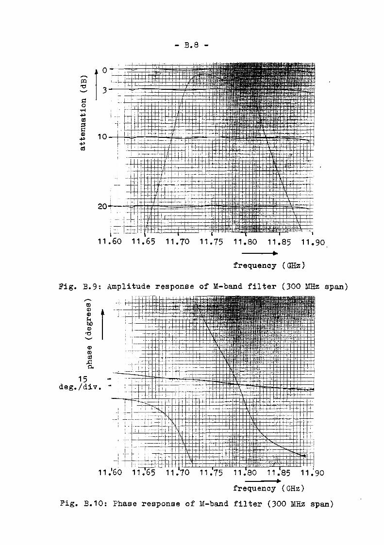
- B.8 -

i~~~~I~lllliill20 .....1~ '.. . .... , .. ,-,-+-.1-

, i I' I

i _1- _, --4- i i, i I· I i I .

i :r-­I _.'.

11.60 11.65 11.70 11.75 11.80 11.85 11.90It:

frequency (GHz)

Fig. B.9: Amplitude response of M-band filter (300 MHZ span)

-lDi r

Q)

OJas~Po

15deg./div. -

,·'1­I

I

11.90

frequency (GHz)

Fig. B.10: Phase response of M-band filter (300 MHz span)

........l=Q'1:l'-'

s::roo0

..-f+:>a3::ss::a> 1...-~

+:>a3

- B.9

: iii'-:...1-+--+ ;...,- f--+- I'. " , , -'" . r"'-'.i ':1-" t:H+h+. I. ,·rH·-I- -,- ...~ -: I ·I-Il'~ .1 __

r:'r ~±tt~tI, ~'}r-t :t-w--t+L~-r.;~r:= : r:--t~· ,-" ..~. ::-r+7~-~~,!,-:L~G-ij J 'l~ T:-=-C r - ~-W- ilt .... -rf -+1 J'i: I f~1' 1:ill'T' :Ii' I . I. ..1..·- +- ... - r I I I2--' ~ ~._: "..~-_. \. - , I , , : I , i I .: I '; , , i 'i l

1. I·J 1+. +--~. ili+'+; .:I:': 'I -+'._L+, :IlimIT. 1_1-- ' -1--' . I '. ., - Ii . ,--, . j T ' I ! I : \ :. +.,- 1 .L., I '. I i

li':- r-,_.', ~.I-lt:I-:~-~ ....L. ,i· I i"r :r'lli .. Lm.':'" ''-,-++ -t-- " : I : ' :~I :t- !:: ,.1 , .. "I I" II I-j--··+I- 1\ I -1--

1i-f-, i ,-;. ,:. : . .j-L i1+H- Ht r-i -1- 'I '-L-II . : l~r"T ~.t'. ,'I'" .II·+-. + . , ·I ., •. ~I1-'- --rJ. ..l...j.' i "1 I - ... '11 I f \-++-1-1 • I+Ii i

.i- i-l,_:_+~ JI+H: I -r;: i-I J+HI- . +1 bit/Jr- "[j ~i4I , L.. L.L~.~.J. r

11:78 11.79 11.80 11.81

..frequency (GHz)

Fig. B.11: Amplitude response of M-band filter (30 MHZ span)

........OJ

1

i +a> -+-.+7-+ 'Q) : 1_··1'~ . L;Q) '1. ~) , :

'1:l .- .

'-' ! l ~:.

Q) I

m -,en

..cPo

11~ 78• 11.80..

11.81

frequency (GHz)

Fig. B.12: Phase response of M-band filter (30 MHz span)

- B. 10 -

frequency lays about 30 MHz lower than calculated.Furthermore the filter is not flat over the wholedesigned band, but it is flat over the transponderband.However, the image band is rejected and the filter can

__~_-+_+-JL-l__i_-I--~ ~____ ; ! __ \l ~~_-:i : , f ' j - -, -_; -- i -, --;\'.L--

__--.:__, B-transponder - _ '. : _-i\ + ~

- ---~-;-l-_b:~_~l-- ~- --,- ---- - --\- ''-, .------:~- --1- - --t--~----- -- --------------\ -. -::~i

20 -----+_-~+_-~.-----III,-----___'t"_TOO+'

.l~~ !_--- .._._~_._~~=~-~I I I I

11.60 11.65 11.70 11.75 11.80 11.85 11.90

frequency (GHz)Fig. B.13: Amplitude response of M-band filter measured,

and corrected with respect to reference lines,and calculated (300 MHz span)

be used. The attenuation is approximately 1 dB (seefigure B.11) in a 10 MHz span around 11.795 GHz. The phasecharacteristic is approximately linear in this band (seefigure B.12), therefore the group delay will be approximatelythe same for all frequencies in the band.

A better version of the CFILTER program is now availableat the Telecommunication Division of the EUT, which givesbetter results with respect to the differences betweencalculated and measured characteristics.

- C.1 -

APPID~DrA C: Local and 5.15 MHz osillator

The local oscillator in the data receiver ~nd shown infigure 4.1, eriginally had an output signal at a frequencyof 11.520 GHz (11. To g!nerate this signal, an external5 MHz signal had to be connected to the oscillator. Thisfrequency was mUltiplied by 2304 to obtain the desire~

11.520 GHz signal.

In order to obtain a signal at 11.865 GHz, the inputsignal'~' frequency is changed from 5 MHz intQ:

11.865 GHz :::2304 5.14974 MHZ (0-1)

For this purpose a 5.14974 MHz crystal oscillator is buildand placed in the local oscillator. The circuit of thecrystal o~cillator is shown in figure 0.1 [JOr.

Two minor modifications are necessary.1) In order to tune the oscillator to the desired frequencya varicap is used.2) A coil is placed in~rie with fue cristal, ~ecause

without it the frequency could not be tuned to thedesired frequency.

With these modifications it is possible to change the5.15 MHz oscillator frequency 35 Hz around the calculatedcentre frequency. This results in a change of 80 kHz aroundthe center frequency of 11.865 GHz of the local oscillatoroutput.

Because the input frequency changes and several parts ofthe local oscillator have a relatively narrow passband,adjustment of these parts is necessary and were carried out.

- C.2 -

Fig. C.1: Crystal oscillator circuit

In figure C.2 the output spectru~ of the 5.15 1llizoscillator is shown. For this measurement set-up B offigure 4.3 is used. The adjustment of the spectrum analyseris tabulated in table C.1.The same is done for the 11.865 GHz output signal of thelocal oscillator, which is shown in figure C.3 and tableC.2.

Finally, in figure C.4 the USB noise band of the localoscillator, measured with the set-up of figure 4.19, isshown. Comparing this figure with figure F.1 of appendixF, one can conclude that, the USB noise of the spectrumanalyser itself can be neglected. Because of this ratherpoor phase noise performance it is recommended toimprove this for da.ta transmissions with small bitrates.

(dBm)- C.3

.-

:'"1=- ~-f Iil:t-;: ~ Tt~ ;:J i1-- t+.~~ r-~-~-~-

-'- '

-10

-20

-30

-40

-50

-60

-70

f"""Iev>ev

f"""I

Mev~o

'Po

-805!14874 5.14974 5.15074

frequency (MHz)

Fig. C.2: 5.15 MHz crystal oscillator spectrum

Table C.1: Adjustment of spectrum analyser for 5.15 MHzmeasurement

centre frequency 5.14974 MHz sweep time 200 sec

span 2 kHz reference level 20 dBm

resolution bandwidth 10 Hz attenuator 30 dR

video bandwidth 30 Hz power level 10 dB/div

- C.4 -

H:r:;TLI

11.8675

frequency (GHz)

Fig. C.3: Local oscillator output spectrum

Table. C.2: Adjustment of spectrum analyser for LOmeasurement

centre frequencyspanresolution bandwidthvideo bandwidth

11. 865 GHz

5 MHz10 kHz

300 Hz

sweep timereference levelattenuationpower level

200 sec20 dBm30 dB

10 dB/div

- C.5 -

USB NOISE MEASUREMENT

l

L-1-~rl--H--+-++1~--t-+-t-tt--T--jH-t-f-­I\I!\IA

, 1 :

l i

~---i--I--l-I-II-\~+--++J-+---+-HTI-r-I--­"'...

--J·I-fT~i.l--4.--l---J-+-+-+--++++--I--t---t--tt----r------1-/1

- I~--+-----I--t--l--+--+-+++---+----t-i--r--r--I- -t-, - , 1

I----/.--I---l-+J--+-++++-+-+-i-H--i---t·,1- --)-- Ii:::IJ_LlJL--l_-LJ-~~~----!'----:;.:--:!:.1-;'''·'----;---;'---;.-;8~1'';'.-~'-~'---;;-.~8tiU.,5 2 4 IS 8105.. I!I 11S;l 2 I;lI

Fig.C.4: USB noise measurement of Local Oscillator

- D.1 -

APPENDIX D: UDconvertor

The phase noise performance of the upconvertor is ratherpoor (see D.1).

It is recommended to improve this by changing the crystaloscillator's implementation.

USB NOISE MEASUREMENT

" 6 810 .. 6 Btl2J" s elil " S 81"

Frequency_ Hz

I

~1-i."--~ I\1\ ~II1yv ·v

r iT1

.-li-;+i'-- - .1-;~t-'\ rt I ,'", -- !;

....... .-.- - t ~....r'\'~~-! H

'~~~ ! ! :

I ~'- -f-"

I-I I

I;

-- I

lJ. . • ,

-14111

-15111121 2 "S 810a

-13111

-12111

-till

-11111

-9111

-1111111

III

-6111

£ -7111"-ril -81111)

Fig. D.1: USB noise band of the upconvertor

(new) (old)724 MHz

724 MHz

+,~

I I3.43 GHz 14.4575 GHz

3.43 GHz

I14.4575

13.73 GHzGHz

724 MHz

Fig. D.2: Recommended new implementation of the

last stage of the upconvertor

- D.2 -

An additional improvement at low offset frequenciesis probably possible if the last stage of the upconvertoris changed (see figure D.2). This was not possible before,because there was no mixer at 14.5 GHz available.The first measurements with a new mixer are promising.

- E.1 -

APPENDIX-E: New symbols for microwave - circuit drawingprogram.

For the available microwave - circuit drawing program[1] five new symbols are programmed.

In table E.1 the symbols are described, whereas the programlisting is given on the following pages.

a e . ew sym 0 s.~ymbol description

8 label: "DCBLKE" lines 863 until 873DC ...BLOK

~ label: "HYBV'" lines 849 until 862HYBRID

~ label: "EYER" lines 835 until 846'microwave swi~ch

\ label: "SCH4.DL" lines 779 until 802' \'"" ' ..." \\ ' microwave switch\

, label: "SCH4DR" lines 803 until 825' ,, ,<II> " ,", ,

I

T bl ---R. 1 N b 1

- E.l -

84t~: ";-;llE:\.IJl:85(1: ·~::.b "E:LIJK H

8 5 i: j=:: 1t 11 +2 • 5 ,E: ~-2

8 5 2 : F,:' 1t A+2 • 5 ,B+2.5

853: pIt A+12.5,8+12.5

854: f=olt. A+12.S,8+15,-1

855: pIt8,-2

856: pIt8+2.5

857: pIt, A+2.S,8+12.5

858: pIt A+2.S,8+15,-1

859: A+7.5-:'-A;8+7.5-tB

86(1: ·3::.b "PUNT"861: A-7.5-:.-A;B-

7.5-tE:862: fE·t

863:" DCBLKH" :8E,4: "3:=.}:,) "E:l:.O~~:1I

865: pIt, A,S+7.5,-2

86E.: pIt A+6.5,E:+7.5~-1

867: r.·It A+6.5,8+10,-2

St.:::: F:Jlt R+6.5,8+5,-1

86'3: pIt A+:::.5,8+5,-2

87~~1: pIt. A+:::.5,8+10,-1

871: pIt A+:::.S,B+7.5~-2

872: F:'lt A+1S,8+

*21207

--A+12.S,

A,E:+

2.5,-1845: H+(115..:.-A;E:+7.5~E:

~: 46: .; :=. b I' PUt·~ T II

~::47: A-7.5~A;E:-

814: pIt. A+7.5*;:.irl (;:.::) , E:+7. 5*1-. ("!~. ( >:;) ~ i f' ( >:: +11 .....24~~<) <=:311.····2;.j f') F=' ~~1

815: P';'fl

816: A-15~A;8-

15-:.-8817: lirlE­81:=:: fE·t.819: "~3TIPDF.~":

8-::'~71: d·:.p "st. i ppeiiijn-ditJ,·3. ;R"

821: pIt. A+2.25,8+12.75,-2

822: 1 i t"J1;- 2, r1 ..···282:;:: F:' 1 t. A+2. 25+

.7*L,8+12.75­

.7*L,-1824: litH'825: fE·t82 tl : II HCI R5 II :827: 5~L; ·~:=.b

"HORL"82:::: rE·t829: "HOR1~j":

83(1: Uj-:.-L;·3::.b"HORL"

831: fE·t.8 3 2 : II HL to( t·~ 5- 1I :

83:3: 5~L; ·:;::.b"HL''(r'~''

::::::~4: fE't.

842: pIt A+2.5~

E:+12.584:~:: F:tlt 8+12.5,

E:+2.5844: ,-,It A+1S,E:+

E:+2.58:3 13: F:,lt.

B+12.584(1: F:'lt.12.5~-1

841: F:'lt12.5,-2

;:; :~; 5 : II HII 8 H II :

::: :::~ 6: '3 :=. b U E: L 0 K It

:3:~:7: pIt A,E:+

F:'E'nB-15-:.-E;1 in E'

1 i n~r 0:' t-Il ::;CH4[iF: II:';I::.!;:. "CIF~15"

7'32 :7 1S':3:7 134 :795: t.. €'t79 E. : :1 ~:; TIP DL " :797: (j:.=.p ns.t.ir.:JF:q:'IIi .j n oj i IJ. .~. ; L "

7'3:::: F=,lt A+2.25,E:+2.25,-2

799: lint;' 2~rI1./2

::: [i (1 : ;:1 1t A+2 • 2 5 +. 7*L, E;+2. 25+. 7*

? ::: :3: d :=. j=:: :1::. C h iJ. k E'

10.0.( 4 s.t'J.fldendio.·'3.;L"

7:::4: A+15..;A7:::5: -1,. ..... 2~>::7:::6: 1 i n€' 2, ~1""'2

7:::7: pIt A+7.5*:=·in(;:<3,8+7.5*c.osC::-::);if (>::+1i/24-:'-~-<) <=0;.j fillO ~~1

? 7 '3 : :1 ~:; CH4 DL II :

7 ;:: ~:i ~ .~ ::. bile I ~: i 5 II

7:::8: F:'E'fl7::: 1

,: B+ 15~E:; A­15-:.-A

7'3t1: 11 ..... 2..;..::<791: pIt A+7.5*

::.ir,(;:':;) ,8+7.5*c·o::· (;:<) ; if (::~:+1i.""

24-:.-;:'1,) <=11';.j ,'IF:' ~:::j

8 (11 :

802:8~:1:3 :i::~)4:

::: ~] 7: d ;:. F:: II S. C h o. k E'

1 'J. 0. r 4 ;:. t G. nd E' ndio.·3.;~:"

t:(1:;": 1 i fJE' 2, r'1·/2:31~:::1: pIt A+7.5*

:=. i tOOt l ;:<) , E+7 . 5 *C(:::' I: ::-:;) ; if" (>=:+1'1' .....2 4 --:r ;:.:; ) <: =ff ':'. 2 ; .j (:'j F:'

:::11: F:'.:'n812: A+15~A;E:+

15~8

~:::13: 'f1'~::'::

8(~5: 15~L

::: e6: -3 s· b II ~:; T rP[J F:

- F.1 -

APPENDIX F: USB noise measurement orogram

In order to measure the USB noise of the various osci11atorsthe measurement set-up of figure 4.19 is used. For thismeasurement a special program is written.

Nith this specific measurement set-up, it is possible tomeasure USB noise band of any oscillator within the 100 Hz- 22 GHz band. However, care must be taken that, the USBnoise contribution of the spectrum analyser itself canbe neglected compared to the USB noise of the connectedoscillator. For this reason the USB noise band of thespectrum analyser at several frequencies is given infigure F.1. A method to measure this characteristic canexist out of connecting an oscillator,of which it is known

-50 .--""T"'T'T....,..,...,.,..,...,.---..T,.......,...,..,....T'M'r""..........--.--,,..,...,...,..,.,...-----r-...,......,....,.,..,.,.,.,

100 kHz 1 MHz10 kHz1 kHz

-70 I-+---'i-....:::,'++++-~I-

!

...-...~~Lt 1'1_ 130 l....-..J......l-U..UJ.lJ._~..l..U..u.u...____L--'-J__I...!..J..l..U-----.l............~

100 Hz

- 110 I--+-+-++t+t+\------,I-+++tt+tt---+

--120 I-+-+-+++++++-t-++++tttt---+--+-i-t+tr

-60

Frequency Offset From Carrier

Fig. F.1: USB noise bands of the used spectrum analyser [25]

that its phase noise performance is much better than thatof the spectrum analyser, to the spectrum analyser.The USB noise of this oscillator can than ~ neglectedcompared to the USB noise of the spectrum analyser,so actually the phase noise of the spectrum analyseritself is measured.

It is also possible to mix the signal one wants to measurewith a signal of which one knows that its phase noiseperformance is much better than that of the signal one is

- F.2 -

interested in (see figure F.2) and which has approximatelythe same frequency. The so downconverted spectrum is connectedto the megsurement set-up and measured. The advantage ofthis method is that the phase noise contribution of thespectrum analysep is redused, because from figure F.1one can obtain that its phase noise performance is betterat low frequencies. However, for the measurement of thevarous oscillators out of figure 4.1, the extra needeqoscillators as described above are not available at theTelecommunications Division of the EDT.

signal ofinterest

noise

1---I

f dphase

1-----1 ~ ,......-...... f df o ~

sourcewith f o + f dbetterphasenoise specifications

Fig. F.2: Set-up for downconversion ofspectrum

In figure F.3 the flow chard of the used program is shown.

In table F.1 the used resolution band widths etc. of theU3B noise me2surement are given. To save measurement time,the measurement ~oints in the first three bands of measurementare linearly distributed. In these bands, the distsncebetween the measurement points is approximately equal to theused resolution bandwidth. In the other two bandslogarithmic distribution is used.

All the phase noise measurements given in this reportwere obtained after. averaging over 20 sweeps, which takesapproximately 1 hour of measurement and computation time.As an example the U3B noise measurement result of the2.6625 GHz oscillator, used in the translator loop(see figure 4.1), is given in figure F.4.

- "7 3 --.

----

11 & 12

program linescorrespondingwi th mentione(block

128 until 190

37 until 56

34 until 36

29 until 33

62 until 127

61

ted

7 -check if plotter, notcalculator and connecspectrum analyserare connected tothe HP-IB bus

connected

mean values of theequivalent noisebandwidths of theused resolutionfilters aresubstituted

1 ---no

~calibration )

yes - --Ir

equivalent noisebandwidth calculationof the used resolutionfilters and amplitude &frequency calibration

....Ir

enter number of USBnoise measurementsweeps

! -measurement of USBnoise, adjustmentof centre frequencyafter each sweep

1 - - I--

calculate mean USBnoise & 1% upperbound & nlot the results ....

~...-

Fig~ F.J: ?low chard of U3B noise me~surement program

- F.4 -

Table. F.1 : USB noise measurement adjustment

offset of bandwidth of resolution number distribution measurementcarrier Imeasurement bandwidth of timefrequency points

{-lS) . "'-.

30-400 370 Hz 10 liz 38 lin. 12 sec

400-1900 1500 Hz 30 Hz 50 lin. 5 sec1900-1190C 10 kHz 100 Hz 100 lin. 3 sec11900- 88.1 kHz 300 Hz 139 log. 20 ms/sample

100,OOC100,000- 900 kHz 1 kHz 150 log. 20 ms/sample

1000,O~C

As said before this result should be compared with figureF.1. From these two figures one can obtain that in thismeasurement the phase noise of the spectrum analysercannot be neglected. on the following pages a listing of

--USB NOISE MEASUREMENT

I!.----- --

L(f) r:}--

I-AI!

-51! \ -\

-6l!I

N -71i1\-.....I,

I

~"-u-911lD

."

~-9Iil

-100'vl-'\ f\

. ,-III! ~

-1211 "-.~

-131! --_.I

-lAl!

-lSI! -- .-III 2 • • 81l!' 2 • e 81&!- 2 • e 9104 2 . e 8I0S 2 . f.l '''n ...,''

F"'.qu.,.,oy. Hz ..Fig F.4: USB noise measurement at 2.6625 GHz with the

translator osc~llator

- F.5 -

the used program is given.

After the initialisation the several parts of the flowchard of figure F.3 are shown.

The subroutines used are also shown.

- F.6 -

4 2: d ::. p II Ad.j .

B ; b e- E" F=I ; 1,1,1 G. i t.3(H30

57: dsp "Connect:::IGt·jAL t.o RF

I t·WUT. "; b;;'E'P;s.t p

5~::: 11:.1 1I::. JJ.I1;d::.p "Put 3IGt·iAL

in 2(a) kHzbl).ndl...1 i dt. h. ";bE·E·p:.; ;:.t. P

5 '3 : r 0:' f", ::. O.6(1: bee'p

B;bee,::'5:3: ,.11 ~ *EG!8~r (

2,30, B, 1,~.n

54: dS.F:: 113~) Hz,Ef~8W i::. (Hz}:",

E:;be'E'p5 5 : c· 1 1 '.;;:. EG! 8 ~~, (2,10,8,1, :::;)

56: d::.p "ltl HzE08~~ i::. (Hz):",

At'1PTD CAL for1(1d8('" .. ; bO:'ep;::.t p

4:3: wrt. "::.o."~

"RC9 HD"4 4: d ::. P "A d j ,_ ':-'~ ,

FREQ ZERO f" 0 r . .;;t~~' .f'lo. X • 1'- ,.... P t, d~. "l';_~i'fX:~)b P€ P •.: t p '... ;"~-)~i>~ :

45 ; d"~;' "1-0 1 ibr:,j,:j;~}• -' pr '\..,. '. ",;.:.~.,:"

tin..; ••. "; 1.')J:t_.,.;~;Ji:

",:s 0. .. , .. KSW" ; i t' .:;:;::- :rd.; ( ",= -1 " ) ; j Pi p "';;"i::;' .4 ,oJ • -" ',',-;::,.~\ :,

4 Eo : d s. p "E G! S\.oJ .';"

co.lcI.d.lt ion."47: ell '*EQ8~·P(

2, 1a(1~3, B, 1, EJ48: ds.p "1 kHz

EQ8W i::. (Hz):",·S;be€r-o

4'3: 1:.11 ~ *Ef!B~P (2,:380,8,1,(:)

5(1: ds. P "30(1 HzEG!8W i::. (Hz):",E:;be12F:'

51: ell ~ *EG!8~·P (2,10(1, E:, 1, HJ

52: aSF:' "100 HzEG!8~~ i::. (Hz):",

rOO ::- d II.:: G. II , A ;

~tc -241: li.lrt. "S,O." ,

I'PC;3 HD"

CAL 0 iJ TF' UT t 0

F:F I f·iPUT. :I; bE'E'P

; ::' t p

J

37

15: dif'" l_$ ['36J ~

t:::$ [::;[1J ; buf .. L ",

t. '/ p .:' 1 = It ~ f:135: if 111:: 1 ; ,~t.~r"' ../

L$,3

14: dif'i F1[:~:J~

"::'IJ.II ,IIT8 11

2E.: for t~=l tel477

D [:3] ,~~ [:3J

17: cHI'" R$[l,:::0]18: di(,', T$[1]1'3: dif", P[477],

G [477J , 'y' [477],GH477J

25: "F'r(I·~rlJ.f'·1

s.t o. rt::. rlE' fE' ••• u

22:23: eli '(;clr

"s.'J.";110 7;wrt.

:::: 13: VI ( t .. :=. :J. " ~

It T ~:; E 1 t:1 A II

20:21: fl\·I\. ;t";.::d 2

:;~6: -gto 57:37: I.~ t" t '1::. o. II ,

lieF 1~:1(1 rI1Z~:;P 1

2:::: nE'}::t H2:3: -:3[1.5.-:rE3~J: -25.4-*C:31: -2~316~H

:32: -i5.:~~--:+~·J

:::::3: -1 (1.1-;.:::;; bE'E'P:3 4: E' n t II For

24:

1 •.. .

8: "(plot.\.E·ro n 1of) b (! I.,j t'"t (j~. II :t :

'3 :

S 2 1 ~3 2 Sf II :

6 : I' l,A ::. E' d f' i) 1'-

::.j'I',C1CIt. h i (1'3. ThE'r6·::.,,,~1t. i:.=. r::l(it~.

E'd ClrJ tt"IE' :::566A~:; F:: E' C t r !..~ (I'! ":

7 : I: G. n G. 1 ':{ :,:. E' rlInd '3::i7::"A F 1ot t.~. r ~. (! .:;. S' t. h E' r-1.,.1 i t h i r.:=. 1\iJ P F=: E' ( (1. n (j 1 (I !.:) E' r

" ..

II :

5: " rIJ.n'~E· -1[1dB (" t. 0 +20 dE: (" .

Di .~ i t G. 1 G. J.... E' r" 0. '':'

in',:, (I'')E't" 100

-1 1: I' e5 6 6 A :I : dE' !.)

H Ii"" 1 ("'I::. 0. 'j' J. I':.

12: u 9:::72A 11 : dE'I.)

"'~F::" ~ '7l15; P:=·C

7~:::15; d if:', H [2] ,H$ 50 ~ >::$ [3~:1J ~

'/$ :3Ci

o: II F' HAt·~ 0 ;: ::1 Aut h 0 r :

::. i",! E' E' f:l :=. i;. 11 :

2 : II T t"l i::. F:l r '=' ":;I r (1.

ft', fl'l E' G. :=. IJ ~.. E' :=. {J SE:no i SE' s· i deblJ.nd::.

,)f SI)IJr::'E:=~

connE·ct.ed to ":3: "t.hE· j;:~F Ir~PUT

IJt" lIn E:566AS to' E' C t r IJ (', An 0. 1y;:.E' r. ThE' o::·c iII Cl.

tor t" fE·'1.IJE·nc·t":4 : II (,'! IJ ;:. t. t1 e- i ~-i

thE' r'J.n·::1E· 130Hz t,(t 221:;Hz;t r-j ~. iJ. f", F:' 1 i to tJ ci E'

("1 U::, t, bE' in thE'

- F.7 -

F' un - Z+2 • 5 +~:;~F' rt·~]

1 (1 ':" :

"Et1 RL 0 Or'lAIA3"

t 'J 477

1 (1 :::: f 0 [" [.j =1 t. (I

477

477

110: nE·}::t t·j111: for t·j=39

t 1:ll

8 :::'112: p[t-n-Z+2.5+

l·HP un c ,

11 :3,: n E'):: t. t~ " .','114: t,'J r N=S:9,.;..

t I~' 18 8 .' .f,~. ",' ,·~1;0.;'~·115: P [Nj -Z+2,.'.~t~~~.

1~ 2~ G~ ~ x t A',' .:<iH~;:~~~~ ;117: t' 0 r N=189:';'"-;';'';§

t·o 327> ',:,,:;;-:,;<t~ql~

1 18: P [t-j] - Z+ 2 .' 5 +i~c;_,C~P CNJ ,- ,,;/);.

.. , _ .... '.-'

11'3: next N ,'.120: f (, r t'~=328' .- .• ,'

121: P[t-jJ-Z+2.5+E-*P CH]

122: nE·}::t. N123: for t·j=1 to

477124: tnlCF'(t·jJ>

10) Hl125: t'l+G un -*G un

; t1l 2 + '0,,' an -* I,,.. un12E.: rIE·>::t. t·~

127: t"l2}::t, --'

128: for t·j=l t.o

132: l(H:lo':;l(GUn) -*P Uj] ; i t"lt ( 10(10+5*P [t-j] ) -*F' [N]

133: it' pun<eq(HF' Uj]

134: if P[N])100'(1; 10~](HP [H]

135: t"lE·::{t t·j136: d:=.F:' "RESULT

1:3:3: I.•J ri:. II so. II ,

S II; bE'E'r.:'1:~:7: 1.I,Irt 11::. 1).11,

129: G[HJ/l-*GUn; ',.,' [H] ..... 1 ~I,,.. [t-.lJ ;f'lbs (',,.. [N] -G un l2)-*QUn

13~:::1: nE'::{1', t·j131: for t·j=l t,:,

:=. IJ. :: ,. '.' +.:: '.'::::3 :

F' U; + 1 (' (']10 2: ri E' ::{ t t·~

1 (1 ::::: 1",1 r til::, IJ. .. ,

'31: rE';] ";:-(1.,

p un'3;2: n ,~ ~ ['i

"FA",U+400,"HZFE:",U+19~30, "HZR8~0 HZ 52 TS"

8'~;- I,oHb ";:.IJ."~

. Ci:3 [IA20 t(~3U,

126,112(1, II

'3 0: f (I r t·j = :~: 9 t c'

"FA",U+1'3~](1,

"HZFE:" , U+ 119~:::1t1,

"HZRE: 100 HZ

II FP ~ U, II HZ F E; II ,

T::; MW'·

1~]5: t,Jr-t ";:-(1."," CF .. , U+ t, n l ( 1'1 ....15~)+5), 11HZ 82

T'-' ..- '-

87: r,E·}::t t·~

8:3: wrt. 1t::. 11 11,

F' ctH327J

F' un:3 6 : r' E· d '1::. IJ. •• ,

"F'E: 1 t:::Z"

9 7: n E' >:: t.. t·~

9:::: !Alrt. II::.IJ.",

u~~E: J[1~3 HZ:3P ~3

HZ ~; T 2 t1 r11~:: F:: L,.'.:"""7 _ ':1 Cit 11 [11"11 ':. ':1-- T I:' II~ .:.. p;J , I. I ,_'':'' ._1

r,I;': fe,t- ~~=12 t.(1

15 (11~](1: 1.'Jrt ";:.,).",

" CF " , U+ t n l ( t·i ....­15(1+4), "HZ S2TS j"11A"

1~]1: rE'd "::,(1.",

'3 4: I,d t b II::;. (t. II ~

I? .~I ~ '-'.1 ( t. "::. IJ. II ,

"03 [iAl~:) t:::::;"~

12 tl ~ II 1 (1, II

'3 5 : for t·i =::: 1;& t G

i ~~1 7: ,', ,.:. ',-' t. r'~

T .:...i ,_I

II E 1 ..

"E 1 "

77: '*r'1A'~Z;'*

t:l F ' ~ U7 ::;: 1.&.1 ( t II::. 0. " •

a ~~ L II , Z+ 1 ~3, :: Dt:1 I;

7 .~: 1.t.1 r t 11:=. ;J. 11 ,I; CF 'I , U, II HZ ~:: F' 2~<Z~~8 1(i~1 H: ::;2

:: ~. E: H2 ~~ L .. , Z ,

7 2: 1•.1 r t II:,:. IJ. II ,

" F.: L " , 2 + 1 (1 • "[I r'1 "73: for ..1=1 t,o 17 4: d :.;. p " C (1. 1 i:' !.~ 1 o.

tin-=:t ~.r('1.CE·: ",--,7 5 : l,J,I r t '1::. IJ. II ~

II CF II , U, II HZSP2 ~] r< Z ~: L .. , Z+ 1 [1 ,IlDt11RB :3~~1(i HZCT :32 T

7' 6: iN r t _.' :J. II ,

r'lF' ~U

'1:- '"c..l;::~ 1: ~ * flO; F ~ ~ u; , *

JI1A' ~:

" E 1 "

" E 1 "64: 'H'1A'-*Z65: wrt ";:.11",

II E2 ~::P 2(1 I<ZRL II

,Z+10,"Dt'182TS"; 20t100-*8; ~)-*.J

66: '.'.Irt ";:.;).",

67: '·:H1A'-*Z6:::: IAlrf.. "::.IIn~

"E2 F.:L",Z+10," Dr'l "

69: if (J+l-*.)) <=1; E: ....·l ~J--t8; i,l.! rt11::. 0.11, "Spit, E:~

I; HZ II ; .j (.', F:I - :370: I,l.lt·t 11:='1).11,

::' 1: .;' n t 11 En t. ~:' r ~

n IJ (:'1 ;::1 E' r Ci f :=. !.~! E' E' P:=.: II , I

c,2 : d ::. p f. \' 0 lj

C (I. r-I r E' ::. t.. for II,1*1.5, "f',in.";t:E'E'~

E,:;:: 1,l.lft "::.!J.1I~

1:39: for t'~=2 t.e

1 4 [1 : 1•••1 r t ";:. G.., ,

int (20(H' (10~ UH­10+2~::1) -1) I, P ct-iJ

141: nE·::-::t, H142: for t·j=l to

5014:3: l.e.Irt ";:.0.",

i nt (2~;:i(B' ( 10<:1 (t·j-:f:30+4~30) -1)),

PUH3:::J144: ne:>::'t ~~

145: for ~j=l to100

146: IAlrt "::.0.",i n t. (2 0·(H· f 1 ':' 9 ( t·H­100+1'3(0)-1)) ,P U~ +:3::: J

147: nE·::<t t·i14 :::: f I) r t·j = 1 ;2to 15(1

149: 1.•Jr-t "::.(1.'"

i nt I; t·HH ,:~::~::3+

6~j1), F' [t-j+177J150: nE·}::t, t·1151: for t·j=l to

150152: :...Irt. 11::. 0.",

i nt. ~ t·~* 1 • :~::::::3+

::;~) 1) ,F' [N+32 7 J153: n.;·::-::t t·j154: d::.f:' HFlo.c.;:'

p IJ. P E' r 0 rl F:l 1 Cl to t E'r f,:,r pl(lt,";bE' E'/.' ; ::.t.~?

155: u F '-~·(\l..~E·nC·i'

Hz II ~::<$

156: IIdE:c. ..... Hzll~\I$157: .. U::;8 t·W I ::;E·

t'lEASUF.:EMEt·jT" .-;.H$l C"-" -'1 '+I-'R~rl'

,_I ::1. i_, 1 _ .:.:. ~ ":. 1-

f-15~3, ~J~ 1~1' 1~.:J~

1 (10J21E100)15'3: PE'n# 4160: f,:,r .J=1 to

2161: ell ~*LPLT~

( :3 ~3, 1 ~:i *1 (1 '::I ( G [ 1]J , - ~ )

162: for- [·{=1 t::~

16:3: ell '*LPLT'(t·H-l ~J+2f3, 1~3*

10 '':I ( Ci [t-j] J , ~) )

16 4: n ~ ::< t. r'~

- F.8 -

50It-t,: ell '*LPLT'(H*3~;:i+400, 10*10':;1 (GEH+:;::::J ) ,D)

lEI?: nE'::<t t'416:::: for t'~=l tl)

P)[1

16'3: ell '*LPLT'fH*1(H)+l'31313,10*i'o':;I ( G UH 8:3 J ) , ~3 ) .'

170: nE·::<t· t·~

171: for H=12t,o 15[1

172: I:.il '*LPLT'(i nt (t n·f (t·V 150+4)), U3*11)'3 (G [N+177J),0)

1"73: ne::<t. t~

174: fClr t·j=l to149

175: .:11 '*LPLT'(int (t.ntCt·1/1513+5)), U3*lo'3 (G [N+:327]),13)

176: ne::<r, H177: ell '*LPLT'

(1 ~::1e113~)00, 1 ~3*

10'; (G [477J), -1)17:::: d=.p II TI:'

.:ont i nu€' F:' rE'::.::·COt·n I t·WE, "; b€'E'P; ;:. t. f'

1 7 '3 : i f" J =2 .. ..1 II', PC',_,

1:::£1: cl::.p IIContinIJE' for 1~'~ UF='P€·r

bound. "; b"".:-p;;:, t F:'

1:::1: for r'~=l t·o/­477

1:::2: Ci [t'~J +2.326:34 7*Q Ct-D "'Ci [t-j]

1::::;:: n€·::-::t [·11::::4: n.;·::-::t -'1:::5: p.:'n#lE6: E'ndl::~7: E'r:d1 ;:: :::: E' n (f1::: 13 :

1 '3 (1 :

191: .. ********~*Subr-o ro'9 rIJ.(··'S **

********":1 132:1 13:3 :194: "*INTERRUPT

" ..1'35: if nl)t, bit'(

E., refs ("so.") +R);.9tO -+5 .<

1~ ~ ~9:i ~ ~ ~ t ( \1:~ :'j}j~~~1'37: '. if bit (3 ':"4' ·L,'

R) ;-'''dsp "HARDl-IAR>;E BROKEN! "; 9t}S:',<.:, ~+2 '.. -: ••... ~

1 '3 8 : i fbi t (, 5 ",""::- R);dsp "ILLIGAL

COMMAt·W! "199: beef:';st~ ;eir 7;iret,

200: eir 7;iret2131: "Et-W *INTER

RUPT n :

202: "E~W *INTERRUPT" :

203: .. Et·W * INTERRUPT":

204:205:2~)6: .. *GRID.·..·*

LPLT":207.:' II HP :::5:::61­

10003, R",,'.} A,7'j07~31":

2~]:::: IICLL~=.: *';GRID ;:.':0.1.;';:.,dro.v)::. o.nd lo.be·l5 IJ. '3rilj ont.he '3:372E: F'l,)t.tE' r • t, :

2~)'3: " ThE' '(-o. ::< i s i::. IJ. 1 1.,.1 0, ./ ::.1 i r,eG. r; t h",' ::0::­o.>::is cO.n bE'

E'ither lin",·c.ror 10''3,'':

210: " LinE'ar·':Irid::. lJ,r",· plott,.;·d orl 1.~lith thE'F' 1 1:, to t. e r F:: 0 t'l ' s, r-o 1 t' ;:. t 'J. t. el"'J1:'nt• II •, .

211: " 10'3 ~rid

::. l.oJi t. h Co 1 1 ' *'LP.LT',":

A f:..::d·····flt fO(f'IO.

tis ::. E'~· to

" ..21 :3 :214: "*LPLT":2 15 : II p 1 , F:' 2 ,

F:' :3 = >:; ,''(' I... ' (1. 1 IJ e ::. ~

PE'n cc,de- t,:,rLOG pIt.":

21t.: pIt (lr:I~(pl

)-HClJ )/H[2J,

217: rE·t.2 1::: : '.' E t·W '*' L PL T "

21 13 :22 (1 :221: II*GiRI[!II:222: II LOG ;:.=:-

rJ.::-::is: ::.PE·C ~1­

F=IS II : :

2 2 :3 : II L I ~~ >:: -o. ::-::i $.: ::. F:J E' C 1:' 1 ­f.-6 for :3tIJ.rt......::;t OF:' 1G.t/E·l::." :

224: II

for CF ..... ::;F-·'J.n1lJ.b€· 1 ::. " :

2 2 5 : II j=:1 1 , F:' 2 ~

F:1:3=\/ ("I i n ~ \1 fiIIJ.::<' #I:! f 1,(' d i ~) ::. 11 :

226: II f:14,p5=>::fl'riri , >:: ('1 G. >::: LI] G II :

227: II r.:,4~p5,

F:I 6 =:x: 1'1"1 in, ::.:: (I"' IJ. >:: , #of ::< di,.'::.: LIH,

S ..... 8 II:22::~: II p4,p5~

p 6 =CF , ;:; F:I iJ. n , 1*o f ~< d i '...' s.: L I r'~ ,

C: F ,.... ~:: F:' G. n II :

2 2 '3 : 11 p 7 =1 ~ -2 , :3 ,4 for C::- in Hz.,kHz ~ r'1Hz ~ GHz II :

23(1: II r:r8=1,Z,:;:,4 f 0 ~- ::; F-' o. n i nHz~ kHz, r1Hz~ GHZII

'PS.C'; <::lifO' H$,>::$,''1'1$; E$; ~\:

ERF:" :.., .:: .:' ..:...._1 '- •

- F.9 -

127-tF-'28 for:=.(11 i d II: 127';"p2:::;:=:-:.-p27

2::::4: if r.-O<5 orpO>8;ell ~.GEF.:'

UJ2:~:5: ':;Ist, II. 'r'PA~: u

2:~:6: F:1c.lr;lbl II

U;pen# l;ifpt1>5;'3tO u_Llt·~u

2:37 :23:3: II_LOCi ll

:

239: ::.cl -.12,1 • 0 4 ~p 11 -. 1 f:' 1 '3 ,p12+.07p19;lbl

24~3: dr-nd (p4,4)-tp14;drndCp5,4)-tp15

241: if F:J14<lE'­'3 ,:,r p15>lE''9'jor ro14>=p15;ell '.GEFU(S)

242: 1("3 ((t.n'tint(10'9 (p 14) :1 -tp22)*int (p14·.... p221-tF-,l?)"'H[l]

243: lO'3(((tnlint (Ie,·;! (p15)) -+p26) *-int (-p15"'"p26l -tp18) ..... p17)-:.H [2J

244: if H[2J(1Cd" H[2J>P:1;cll'.GEF.:'f'9)

245: p22(F:,17/p22-1)~p21

246: drnd(p21~~·.

p 22+ 1 , 2 ) ~ F=' 2 S';if F:-23> '9; 1-:'102:3;1 [1F:'22~F=:22

247: d rrpj (f,::23p22

24:::: if H[2J)5iJ.rld j=:' 23#1 tJ.~·icl

p2:3~2 IJ.nd F=1 2:3#5;·~to +7

24'3: if H[2J>2'Ind H [2J <=5iJ.fld f rc (,::.2:;:/2) #0 'J.nd F:·23# 1 ;'3t 0 +6

25~]: 1 i rl~ j=:' 27 ,F=I 2 :::; i f p 2 :3 =1or 1Q21=r.'17 Or

251: ell '*LPLT'(r;'21,r::1 12, 1);ell '*LPLT'·r,·p21, pi!, 2); F-'E'rdf ::< d ~:1

252: if 102:3#1;e s,'i z 1; c pIt. ­1.5,-1.Ulblp23; '3t (, +3

253: c::.iz 1.2; .,c.plt -.:i- (p22#1 '.: .

and p22# 10) ,_:;:::~:: ~1 ; 1b 1 .. 1 U • if ·;:fii;';'. 0.

, .0 .0 L.l;;,-

2 2 4t 1 • 1b 1 :~.... r.:l ..; :.;/,[ <.'-,"1:'.'p '11" _ : • '<'{,/ ."._ < .<.;:",,;

254: if (lo~(p2'2<>i5~

) ~ p 2 5) # a 0.nd " .~<; ~

P 25# U Co s i z • 8; '>';"0cplt - (F=l25Y0) ,'::.:,::0.6;lbl p25

255: if p21(p18;''3t.CI -9

256: 0-tp14; 1~p15;.5-+p24;"3tou_XLBL u

257:258: II_Llt·~II:

259: p4-tp14;p5"'p·15; into (p6) -tpn:.;if f=l0<7j·;!to +4

2t,~3: P 5.·'"2-:. p 15; ­p15~p14

261: if (int(p7)-tp17)(1 or ~17>

4 ,jr (int(p8)-:.p1;::) <lor p18>4;ell '.GEF.~'(5)

262: if ~16<2

or fre(p16.··.. 2)#t1;ell '.GEF.:'(6)

263: (r-·14+p15)/2-:'p24

264: if (r-'15­p14i'F:'2(1) <=~3 orF:·16<1 or plE»25;cl! ' .GE~:' (7)

2 to 5: "~So C 1 P 14 -. 12f:'2(1,p15+.04p2(1,pl1-.lr-019,p12+. 07pl'3; Ibl

p21Zt,:3: line p27,

p2S; if p22=0c,r ,,22=p16 orp0>6 IJ.nd p22=p16 ....·2iline

- F.10 -

322: fE"t

323: "nw *CiRID"

314: ret. r:02+2315: ".ULBL":lbl .

"";if p1#1;1lb lch (I, r ( 1a7- ( p L,:I;i ~ :I~~~ ~ =~} +?:::>;;jr:

316: lbl "Hz" -"t317: ret -'~t

~ 18 : ". 'i PAR" : d r nitI

d(pl,5)~"lU i

drnd (p2, 5) -:-F:'12 f

319: if (p12- I

r::'11+r:01'~) <=~);

cll '.GER'(2)32~3: if °o.b::.(p11)<.~)e1 CI.nd pl1#0or abs.(r-·12){.0

~)1 and p12#0;c.ll '. GEF.~' (3)

321: if (int.(F:.:3)-:-p13J <1 or ~13>

25;cll '.GER't:4:1

311: t-E·t F::2312: II.GEF:":PE·n#

; II *GF~ I 0 II ~E$;

-11 ,.:.:.r-pc,: "~"1'1''_. . .. c:. '. ,.... I.• J .,

t- ;::. t.

P 1# (1 ; 1'·l'J. X ( 0, i n t (10':;1 ('J.b:=. (p1)))) ~

32:::: lIeLL: t'1I5'IJ.::.I.A

t- e' E' ':t IJ i 'v' n 0 i s· E'or ij,·,pul:::.e· 8l~

31:~:: II.ILlI:if

1~~:n311, Re-'.) R,79~3701":

clf 85t.6A II:329: II p1=Co.1-

L··F:'E' (1 =I j')PlJ 1s·e; 2 =t·~ (I i S E') II :

33~): II p2=RBt.o c'llibrlJ.te-,

324:325:3 2 6 : " *EQ E: l·J " :327: IIHP ;::5861-

Bl·J, Hz":3:33: .. [iC5J =Cl:' r r

e'ct1c,n f'J,ctor(to F.~ef Bl·J),dE: (R)":

Hz II :

331:" p3=E',::tIJ iI.) BW, Hz (RJ":

332: " [f:l4J =Ref

2 132 :293-: a _ '/ A::-:: II : " 11 -.:.

4

F:·21;fHp22294: 6-jf,O,X (' • I L'1:F:'11),~.IL' (p12) )-:-p25

2'~5: f ::-::d j ... i n (1"'0.::<('.FL'(F:'11),, .FL' (pl'3/pl:3)), F:·25) -:-r.-lfi; c::.iz

296: line p27,'::12:::; i f" p22=~

or ,,22=1='1::::; 1 ine'

297: pIt. p15,p21~liF:'lt F:·14,F:,21,2;r.-.:-n

29:::: cr.-Ii -(1.5+p1(1- (t:010=~~1) +'.IL'(p21))~-

• 1 ; 1b 1 p212'39: if (p22+

1-tp22) >1=:11:3; ~ti:i

2::;13: c::.iz 1.Z;f>::d p10; 11::r1n (II, F:.2:~;; ::.11, • fJ L E: L' I; p ::: J ;

3~) 7 :

304: f:llt (p15+. 1;:,20) (p~Y>5) +1 . 1 (F:'0=5) , P 1, 1 ;

1 .-,.~

Ibl" .····OI'·... ) ..2 '3 ~J :2'31: lI_HEA[llIj(.:=.i

z 2;plt. p24,p12,1;cF:'lt. ­le'n(H$)/2, .5;1b 1 H$

305: f>::d 2;c~iz

:;~~:::1'3: n a FL II: 1 ~3";'p2

310: if p2>0tJ.nd F:'rnd (p1, 1­F:' 2 ) :: p 1 -;"':1 2 - 1 ~)=:I 2 ;j (:'j f:' ~3

+3:3~3(1: P t"t"jiJ (p 11 +

)=:1 113*~:22/p 1:3,-F:' 1 (1) -:-F:'21 ; ':;It. ':' -4

3 ~J 1 :3 ~j 2: II _ I";"' LE: L II : EJ_.l·t

p14, (pl1+r:::12) .....2,Ucplt -(p10+6.5),0

3~3:~:: c::.iz 1.5,2,1,'30;cr.'1t.. -lE'n('-($) /2, ~3; Ibl \'$

27 13: p2~3""'F:' 1tl"*p23; (l'lin ('. FL' (F:'23),p10+2'F:'25+2)-:-p10;f::-::d F:i1.3

2:::~]: - ('. IL~ (F=12:~~

) +r:'l~3) .····2-:;:~p25;

if "~~1>6;·::;;\.o

"_CF"2~::1: cplt~ p25,-

1 ; 1 b 1 ,::: ~: :3 ~ II ./

DI \:111

; ':;It. Cl II _>::LE:L

27:::: F:'It. '::124,

pl1,1;csiz 1.2;

E:L' (p7)

z 1.5;r.-lt. ;:,24,f=, l1,1

2;::e: cplt llSf.p25-2) (p~»6:1-1E'n (>::$).····2~-2;lbl ::<$,U u;if iY(i(7;

'3t Ct "_HEAD"

269: '::1 t F::21~

p12,1 f;:lt. p21,pl1,2 if (,:::22+1-':'p22 >F:t 16;,::;to+2

27~]: p14+p2~3~*

p22 ...··p 16~,::'21;

·:;It.o -2271: r.,It. r.'14~

2 ~:: 4 : f >:: d '. FL' (F:'4)";'p26;cplt ­('. IL' (r::'4)+r.'26+12)/2,-1

2;::5: 1b 1_ 1I CENTE~~

= II , f== 4 ; I:. 1 1 '. UL

272: f >~d fIO.::{ (lIb::.(r.o14) ':::l~,'. FL' (r.·14)) -:-r.'25; lblr.o14

27::::: if f='~»6;

ell '.ULBL'(pt:)274: f)<:d 1'·I'J.::«(;lbs.

(r.:d5) <10,'. FL' (F:'15)) -:-r.ol~3

275: pIt. F:1 15,F:' 1 1 , 1

276: er.olt -2 (p((>6)+(p10=~::n-'.IL, (p15)-FJ1t1,-1;lbl p15

277: if P~~1> 6;ell' .ULBL' (p:::)

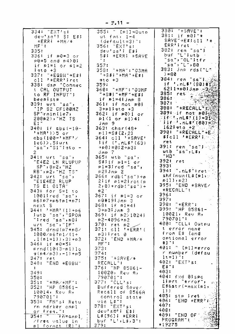
- F.11 -

1'1 F " :

,t -I

,fII/.

I~ .

39E. :3'37 :398: u*ERRu:3 13 13: II HF' :::5:::& 1-

10021, R,:·,.} A,79(17~:11 .. :

4(10: "eLL: Output e·rror nO.l"lef rol"'t E$ [o.nd(,Pt i orllJ.l e r t"(1 r#] " :

401: " [pi] =error nl"H',be' r (def o.UIt.=1)":

E$" :4 (13:404: f>~d f,; ::·~c

1 ; p r t "e- r r 0 r " , y·'"f;

E$~dH r (-J'·ltJ.>~ (p 1, ,.}1))

4 (15 : .::. t P ; r» t . ::.;" :- . - ,-, ~.,,""

4 ~3 6 : " END *ERR !' :'

407:408:4~j9: "ENO OF'. ',-y,~;...~..

PRI] GF.: AM" : ' .. ;::~~:'"

*19275 .

3:::[1: :a *::;A'.lE":3:::1: if P(1;"*~3AI'/E"-:+E$;c.11 '*ErU~~';ret

3:32: rE'I,'1 u::.o.u;buf "L";IJJtb ."::;.0.", "OL"; t. f rII sa ","L It ,S0

383: .j ("IP rds (" L'")=80·' . '

384: re!'", "sa''';' ,'~~~:"if' • n L $' (8 0-) fd~~~;;7 '62; 1~ p 0; ,j PIP '.~:3"

385: r e.t; ..:.- _";.1";~386: ' .~~...;.387:388: ... *RECALL\'I

, 389 : if not' ,peJ-· _~_ ;:: if-'· '. nL$': (1 j =gifr~; i

. ; if' • n L $~" (8~ r:i:i~~i :162; ":It. 0 ,+2"',-. ,~:,;:2>, ,1

39~P "*RECALL" ~E_:t .:$; ell ' *ERR'; , -::"r-e t..

391: refit "sa '.' ; .'wtb "sa",L$,"HD"

392: ret393: _394: ... nL$ .. :ret····'­

shf (nul') (L$ [p 1" '. '.p1]),F=·2)

3'35: "END *SAVE/*RECALL":

:355: " [pl]=CilJtpIJt f,,·,t, 1-4(d.:·f IJ.IJ 1~, =3 J ":

35tJ: ltE>::T'::.:d.:·;.)' ::.0.'; E$;~:;$; *E~:R; *SAI',IIE

~:ECALL" :

357::35:::: II *til A ": "IJ:3~lA

II ~ S:$; "* r1 A II -:-- E$ ;":I t. 1:1 +:;:

359:

" ..

:360: "*t1F":" O:3t'1F"~S$; "*MF"~E$;

if 101=4;j(iJp 8361: if n':lt 100;3~pU":lto +3

362: if 1:'0> 1 orpl <1 or pl>4;j,»p 9

3E·3: (.hlJ. r (48+pl)~S$[2,2]

3 E. 4: c 1 1 ' '* SA'.l E ';it' ('.nL$'(63)-:+p(1) =0; 2-:+p:;:;.j "'1 P 7

365: I..Jt,b "::.IJ.",

S$; if pl=l orpl=3; rE·d '''sa'',P2;ji",P 2

3E.6: rdb ( .. ::;.'J.")-:+p2; if pl=2; rl:,t (p2 ~ :3 ) + r d b ( II S. Cl II ) -:+F:1 2·

367: if 101=3 orp0#1'3;.jrrJP ::::

368: if 101=4;3-:+p3;.j,YIP ::::

36'3: if p2> 1024;p2-4£1'36-\!ot-·2

3 7 0 : r e' t. p 2 ~/

371: ell '*ERR' (p:~:);rE·t. 0

372: "Et·W *t·1A ...··*t'l F If :

37:3 :~:74 :375: \I *SR \11 E.·,"i-

37E,: "HFI ::i5:::IS1­1[H:12~:1, R.:·'.... A,7'30701 ":

377: "elL'::.:Buf f E' r.:·rj ~:;IJ.VE·"·"

~:E·c.o.11 of :::566Aeorltrol ::;·t.o.tE·

I.'" i IJ. L$If:37:::: IIE::-::T':=.:

de'I.} , s'[':-~; E$;L$ ['36]; *ERR;but' 'L',L$,3":

379:

" * t'1 A...·· * 1'1 F " :

1 (a:1 1 4 , RE' !.... F!,7'3(17(11":

3 5':~: : u· F t·~ , ::.: RE' t IJ

rn I"!o:rker o.r'IP1(I r f t'" E' ':t. II :

3 54T--"- --l r:l-=0: i') P 1,.····f re'l '.)," IIJE' inp1 fori"".t fRJ":

3 :~: 5 :336: if' F:'~J=3 ot"p~)=5 (I.nd P4>~:1;

if pl=l Cir F:ol=2;·'3t.o +3

337: "*EQBl·~"~E$;

.:.11 '*ERR';r.:·t338: d::;.p "C':li'"1nec.

to CAL OUTPUTto RF INPUT";be'e~;stP

33'3: I.~I rt, "so.","IP 82 CFltHH'lZ8P" ;r I» i n ( 1 e 7 ,200~2),"HZ T~3

El"340: if o.b::.f-l(1­'~H1A'»5 oro.bs (10~3-' *t1F' .....lE·E.):::-. 5; 1••Jrt.1I:;.IJ.

II ,II::;l l1 ;'::I'l:.CI -2

341: '.~Irt "::;.a","E4E2 L~l RLUPUP

3:34: "E>::T':=.:1::1 E' I.} II ~. IJ.' ~ ::;; E$ ;*ER~:; *i·1A.···*

350:3 51 :352:

::;p", :3p2, 11HZRE:",F=,2,IIHZ T::;II

342: 1.,.1 ft. II::.IJ.","E 1E4E2 ~:LUP

TS El CllTA"34:3: f,:q- 8=1 t.o

1 ~~H:11; t"E·d "::;.0.",F=·6; p7+p6lp 1~p7;n E' >:: t ::;

344: ' *t'1A' f 1) -:+p6; 1••Jt, b "::;.t.1."," SPOAlI;red uS(I.u,p:::;1•.Jft.. 1I::. 11 ",IIIP"

345: d t"nd (p7*p:::.····1~J00.·..·p6'tp 1 ..··· (1 +.1 fr.ol=l)) ,3)-:+p:3

346: if F:'0=5;r.ornd (1(1 (::::-pl J 10''3 (p4.··.. p3) , -1 J -:+j::·5

347: rE·t.34:::: "E~W *E(~E:l·~"

- G.1 -

A~PFENDIX G: ?rograms to s~eep synthesizer

To control the synthesizer ane has to put the desiredfrequency into a string (Y$). This string consistsof g variables with the following meaning (see tableG.1 ).

~able G 1- Assi~nment of variables to used strin~• - >-..

string varable value output frequency of synthesizer

Y$ 1 .& (code)

Y$ 2 Q.,- 9 . GHzY$ 3 0-9

Y$ 4 0 - 9Y$ 5 0 - 9

- MHz

Y$ 6 0 - 9

Y$ 1 0 - 9Y$ 8 0 - 9 kHz

Y$ 9 0 - 9

Four programs are available. They sweep the synthesizerone from one frequency to another with certain frequencysteps (see table G.2). The listings of the programs aregiven on pages G.2 and G.3.

'1 bl'r bl G 2 Sa e • : weep programs ava~ a efile start frequency stop frequency frequency step

9 11.145 GHz 11.845 GHz 100 kHz

10 11.185 GHz 11.805 GHz 20 kHz11 55 MHz 85 MHz 100 kHz12 55 MHz 8~ MHz 20 kHz

~ G.2 -

file 9 file. 10 file 11

fII .( .(

t,1

,'-'

31: w'lit, 5~3

32: n€"::<t Z3:;:: end~-:3132t1

.' ",~:'5: \. --. -"--- -- '.-.-,:::>-> :

0: "-ixd 0" ----:.. ; ··~'~~i;··~-'I-.'. ,1R(~-d(''2i ]((1 ~ ~ ([~~ J.f;X~:t !, ." ~ , -... C ,-' .. -" ..

"'r$'!2!.. ~.J_ ,~:'~~~:~~":}~l ~2 ~'" H -t ($ (11\;,; "tFf"'C: %

3 :' .. 0 .. -+ Y$ [ 21:-:: '}:'(K~; ,~A: " "l'" -1- Y$ [3] '. - --:,;,~~. :?5: " 'L e"-1- Y$ [4] 2"':, ,:

·6 : " 5 " -1- Y$ [5] , .'7 : " 5 " -1- Y$ [6]8: "0".,..'-($[7]9: "0"-1-'"('1 (8]"10: "0"-1-Y$[9].11: Wrt 725, "H11

'. 745000"12: wrt, 725, "00"13: wrt. 725, "t'~03

00"14: f,:.r Z=551to 85~3

15: 2-1-\'16: st.r(int.(''(/

P3(1) ) -1-F.:J: [1 J17: Y-I.}(1.1(F,:$[1])*1~3~3-1-'r'

1:3: str(int-f;''f'/1(1) ) ""::;$ C1 J

1'~: $.t r f "(-'.... ,11 (::;$[1]) *P3) -1-T$ [1]

2(1: "H"""\($[lJ21: "0"-1-"($[2]22: "0"-1-"($[:3]2:3: "~)"-1-\($(4]

- 24: R$ [2] -1-\'$ [5J25: S$ [2] ",,'/$ C6]26: T$ [2] -1-'/$ [7]27: "(1"""'r'$[S]2:3: "0"-1-\'$[9J29: wrt 725, '($30: wn. 725, "H03 ~,

00"

Ii 1 II ~ Y$ [2 J

I.\i rt- 72:i, Y$t.,,! n. 7 2 5 ~ .. t·~ 1(1

"1"""'($[:;:]Q$ [2J -1-\'$ [4]R:$ [2] -1-\'$ [5J::$ [2J -1-\'$ [6]T$ [2J ""'/$ (7J

'35 ..

',5 II

~): f::<d 01: diff \'$ [l~n,

G!$ [2J , F.: $ [2J ,:::$ [2J ,T$ [2] ,U$[2]

2: "H".,..'/$[1]:3: "1"-1-'/$[2]4: "1"-1-\'$[3]5: "7".,..\'$[4]6: "8"-1-\'$[5]7: "5"-+\'$[6]8: "a"-+\'$[7]9: "a"-1-\'$ [8]10: "(1"-1-Y$['3]11: wrt 725,"H11

74500..0"12: Wrt 725, "00" ."1:3: wrt 725, "tH0

'-1 .-: a":1.:'1 •

"'='7­.-. I •

,?e.'- ._1 •

2 tt:

:35: '))o.it 5~:1

36: nE·;.::t- Z37: e'nd*2~3614

2 ::: :2:3 ::3 ~3 :':1 1 •,...1 J. •. .., '-1 II

,.J ~ •

14: for Z=7:::5~)2

t (, 805~30 b't 215: Z-tll

"J6: strfint('r'/10Iaa~)) ) -+G!$ [1]

17: 'r'-',.I'll(I}$(1])*11~:n)0~)-1-'r'

18: ::.tr(intf'/.····1(H)0))-1-R$[1]

1'3: ·/-'.... ,J,1(R$[1])* 1(10(101'\'

2~:1: st-r(int("(./l(H)))-1-S$[lJ

21: ')"-'.... 0.1(:::$[1].1* 1 (112\ -1- \'

22: str(int-(·'f·.····p~n)""i$(l]

2 :~:: s t- r ( 'r' - I.... O. 1 LT $[ 1J J*1(j ) .,.. U$--rf ]

24: "H".,..'r'$[1]

"~jU-:'-'l$[:::]

II t1 11 --trr'$ [13]

(.,1ft 725,"1'$'...Irt 725, "t'4~:13

" 1 """'-($ [:3JI] $ [2 J .,.. '/ $ [4 Jf':$ [2J ""\'$ [5J:3 $ [2] .,.. 'y' $ (6 JT$ [2J .;.\'$ [7J

.3~) :

31:

3:~:: l.vlJ.it. 50:34: !1E'>::t. 235: lS'nd*1~:1271

21: str(lo(-I.}(i.!(S$[1J )*1(1)""T$[1J

22: "H".,.."($[U

26:27:

24:~C"..:... "..I •

0: f::<:(j 01: dif", 'l$[1(1] ,

G!$ [2] , R$ [2] ,::;$ [2] ,T$ [2]

2: "H"""\'$[1]3 : "1" .,.. 'r' $: [2]4: "1"-+'('$[;::]5: "7"-+\'$[4]6: II 4 II-t

l"(,$ [5]7: "5"""'/$ [6]8: 110 11 .;..1/$[7]9: 110r1~ti$[::~]

1 ~] : .. ~3 II ~ 'yl $ [13]

11: (·Jrt 725,"H11745e~)0 "

12: '..Jrt 725, "en)"1:3: I,,) rt 725," t·H:1:3~)O "

14: for 2=7451to :3450

15: Z-:.-\I16: str(int('/,/

10(H))).,..(a[1]17: Y-'.)(I.1fC!$[1])*1~:10~:1""\'

1:::: ::.t (f int (./,....1(1(1))""R$[1]

1 '3: 'r'-'.... (1.1 (F.:$ [1] )

*100""'/20: str(int(\·.····

.."<~1L----------I----- ---J~ ......:::J>

file 12

10: f><d ~3

1: di""1 'y'$[1~3J,

G!$ [2] , F.: $ [2] ,::;$ [2] , T$ [2]

2: "H"-t''('$[l]3: "0"-t'/$[2]4: "0"-t'·($[:3]5: "121 "-t\'$ [4]6: 115 .. -:-- 1'('$[5]7 : "5 " -t ..... :$ [6]8: "'0" -t''('$ [7]

10: "~1"-tY$['3]

11: wrt 725,"Hll7450~:n) "

12: t,.,1t"t 725, "00"13: I,.Jrt. 725, "t·W3

00"14: fc,r 2=5502

t.:. 850~j b'/ 215: Z~\I

16: str(int(y .....10(0)) -tQ$ [1]

17: 'r' - '.... iJ. 1 (!~ $ [ 1] )* 1 (1t10-t'/

1:::: str(int('r'./100)) -tF.:$ [lJ

19: 'r'-,.... ,J.l (F.:$ [1])*100-t'/

2~): ::.tr(int('T'.····1(1) ) -t:::$ [1]

21: st r ("!"-I')'J.l (~:;$

[1] )*10)-tT$[1]22: "H"-t"($[l]2:3: "~]Il"*Y$[2J

2 4 : II ~3 II -+ Y$ [3]25: "0"-t\':;'[4]26: G!$ [2J "*'/$ [5]27: F~$ [2J ~Il$ [6]2:::: S$ [2] -*\1$ [7]2'3: T$ [2J ,*'/$ [:::]:;:: D: " (1-" -t ''( $ ['3 J3 i: i,l} t· t. 7 2 5 , Y$3 2: !,I.I r t 7 2 5, "t·~ 0 :3

(10 "33: i.,,1!J.it 50:34: tls·>=:t Z:3 5: .;' fit]*:3742

- G.3 -

- li.1 -

APPENDIX H: Application for Digital Satellite Eperimentswith the B-transponder of the OTS

- R.2 - -.­• =Experimenters would like to submit the following applicationfor using OTS transponder B.

1. Objectives

- development and testing of 12/14 GHz equipment for digitalcommunications for special services (up to 8 Mbit/sec.)

- measurement of BER as function of bits/sec. during averageweather conditions

- comparison of some modulation equipment (IF modulator plusup converter/switched RF modulator)

- system demonstration with 2 Mbit/sec., DPSK.

N.B. It is the intention to demonstrate, at a later stage, a videosystem operating at 8 Mbit/sec.

2. Experimenters

Telecommunications DivisionDepartment of Electrical EngineeringEindhoven University of Technology, The Netherlands.

3. Administration submitting

Netherlands P.T.T.

4. Countries involved

The Netherlands only.

5. Signals to be transmitted

5.1. Swept carrier for channel characterization(differential gain and fase)

5.2. DPSK signal 2 Mbit/sec., 4 Mbit/sec.

5.3. DPSK signal 8 Mbit/sec. (optional).

6. Repeater

Module B, channel LR or RL (exclusive use).

7. Period of implementation

One year, 1 May 1982 to 1 May 1983.

8. Total time

8.1. 16 hours during June and August 1982 1> subject to negotiation

8.2. 10 hours during April 1983 J9. Daily times

1 or 2 hours (maximum) once a week during June 1982, and 4 hoursweekly during two weeks in August 1982.One full working day in April 1983.

- H.3 - -.­• =10. Earth station

10.1. Receive/transmit antenna diameter 8 m,noise figure 10 dB

10.2. Maximum transmit power 10 w.

11. Organisation responsible

Telecommunications DivisionDepartment of Electrical EngineeringEindhoven University of TechnologyPostbox 513, 5600 ME Eindhoven, The Netherlandsphone 040-479111, twx 51163 thehvnl.

12. Point of contact principle

prof.dr. J. C. Arnbak, phone 040-473451.

13. Point of contact routine

J. Dijk or A.P. Verlijsdonk, phone 040-473417 or 473445.

14. Comments

Chief purpose of experiment is educational and R and D in the fieldof digital satellite communications for special services.

Eindhoven, 13 January 1982.