eigenvalues and eigenvectors - texas a&m universitydallen/m640_03c/lectures/chapter… · ·...

Chapter 3

Eigenvalues and Eigenvectors

In this chapter we begin our study of the most important, and certainly themost dominant aspect, of matrix theory. Called spectral theory, it allows usto give fundamental structure theorems for matrices and to develop powertools for comparing and computing with matrices. We begin with a studyof norms on matrices.

3.1 Matrix Norms

We know Mn is a vector space. It is most useful to apply a metric on thisvector space. The reasons are manifold, ranging from general information ofa metrized system to perturbation theory where the “smallness” of a matrixmust be measured. For that reason we define metrics called matrix normsthat are regular norms with one additional property pertaining to the matrixproduct.

Definition 3.1.1. Let A ∈ Mn. Recall that a norm, · , on any vectorspace satifies the properties:

(i) A ≥ 0 and |A = 0 if and only if A = 0

(ii) cA = |c| A for c ∈ R(iii) A+B ≤ A + B .

There is a true vector product on Mn defined by matrix multiplication. Inthis connection we say that the norm is submultiplicative if

(iv) AB ≤ A B

95

96 CHAPTER 3. EIGENVALUES AND EIGENVECTORS

In the case that the norm · satifies all four properties (i) - (iv) we call ita matrix norm.

Here are a few simple consequences for matrix norms. The proofs arestraightforward.

Proposition 3.1.1. Let · be a matrix norm on Mn, and suppose thatA ∈Mn. Then

(a) A 2 ≤ A 2, Ap ≤ A p, p = 2, 3, . . .

(b) If A2 = A then A ≥ 1(c) If A is invertible, then A−1 ≥ I

A

(d) I ≥ 1.Proof. The proof of (a) is a consequence of induction. Supposing thatA2 = A, we have by the submultiplicativity property that A = A2 ≤A 2. Hence A ≥ 1, and therefore (b) follows. If A is invertible, weapply the submultiplicativity again to obtain I = AA−1 ≤ A A−1 ,whence (c) follows. Finally, (d) follows because I2 = I and (b) applies.

Matrices for which A2 = A are called idempotent. Idempotent matricesturn up in most unlikely places and are useful for applications.

Examples. We can easily apply standard vector space type norms, i.e. 1,

2, and ∞ to matrices. Indeed, an n × n matrix can clearly be viewed asan element of Cn2 with the coordinate stacked in rows of n numbers each.The trick is usually to verify the submultiplicativity condition (iv).1. 1. Define

A 1 =i,j

|aij |

The usual norm conditions (i)—(iii) hold. To show submultiplicativity wewrite

AB 1 =ij k

aikbkj

≤ij k

|aik|bkj |

≤ijkm

|aik||bmj | =i,k

|aik|mj

|bmj |

= A 1 B 1.

3.1. MATRIX NORMS 97

Thus A 1 is a matrix norm.

2. 2. Define

A 2 =

i,j

a2ij

1/2

conditions (i)—(iii) clearly hold. A 2 is also a matrix norm as we see byapplication of the Cauchy—Schwartz inequality. We have

AB 22 =

ij k

aikbkj

2

≤i,j k

a2ikm

b2jm

=

i,k

|aik|2

j,m

|bjm|2

= A 22 B

22.

This norm has three common names: The (a) Frobenius norm, (b) Schurnorm, and (c) Hilbert—Schmidt norm. It has considerable importance inmatrix theory.

3. ∞. Define for A ∈Mn(R)

A ∞ = supi,j|aij | = max

i,j|aij |.

Note that if J = [ 1 11 1 ], J ∞ = 1. Also J2 = 2J . Thus J2 = 2 J = 1 ≤

J 2. So A ∞ is not a matrix norm, though it is a vector space norm. Wecan make it into a matrix norm by

A = n A ∞.

Note

|||AB||| = nmaxi,j

k

aikbkj

≤ nmaxijnmax

k|aik||bkj |

≤ n2maxi,k

|aik|maxk,j

|bkj |= |||A||| |||B|||.


In the inequalities above we use the fundamental inequality

k

|ckdk| ≤ maxk|dk|

k

|ck|

(See Exercise 4.) While these norms have some use in general matrix theory,most of the widely applicable norms are those that are subordinate to vectornorms in the manner defined below.

Definition 3.1.2. Let · be a vector norm on Rn (or Cn). For A ∈Mn(R)(or Mn(C)) we define the norm A on Mn by

A = maxx =1

Ax . ( )

and call A the norm subordinate to the vector norm. Note the use ofthe same notation for both the vector and subordinate norms.

Theorem 3.1.1. The subordinate norm is a matrix norm and Ax ≤A x .

Proof. We need to verify conditions (i)—(iv). Conditions (i) and (ii) areobvious and are left to the reader . To show (iii), we have

A+B = maxx =1

(A+B)x ≤ maxx =1

( Ax + Bx )

≤ maxx =1

Ax + maxx =1

Bx

= A + B .

Note that

Ax = x Ax

x

≤ A x

since xx = 1. Finally, it follows that for any x ∈ Rn

ABx ≤ A Bx ≤ A B x

and therefore AB ≤ A B .

Corollary 3.1.1. (i) I = 1.

3.2. CONVERGENCE AND PERTURBATION THEORY 99

(ii) If A is invertible, then

A−1 ≥ ( A )−1.

Proof. For (i) we have

I = maxx =1

Ix = maxx =1

x = 1.

To prove (ii) begin with A−1A = I. Then by the submultiplicativity and (i)

1 = I ≤ A−1 A

and so A−1 ≥ 1/ A .

There are many results connected with matrix norms and eigenvectors thatwe shall explore before long. The relation between the norm of the matrixand its inverse is important in computational linear algebra. The quantityA−1 A the condition number of the matrix A. When it is very large,the solution of the linear systemAx = b by general methods such as Gaussianelimination may produce results with considerable error. The conditionnumber, therefore, tips off investigators to this possibility. Naturally enoughthe condition number may be difficult to compute accurately in exactly thesecircumstances. Alternative and very approximate methods are often usedas reliable substitutes for the condition number.

A special type of matrix, one for which Ax = x for every x ∈ C,is called an isometry. Such matrices which do not “stretch” any vectorshave remarkable spectral properties and play an important roll in spectraltheory.

3.2 Convergence and perturbation theory

It will often be necessary to compare one matrix with another matrix thatis nearby in some sense. When a matrix norm at is hand it is possibleto measure the proximity of two matrices by computing the norm of theirdifference. This is just as we do for numbers. We begin with this study byshowing that if the norm of a matrix is less than one, then its differencewith the identity is invertible. Again, this is just as with numbers; that is,if |r| < 1, 1

1−r is defined. Let us assume R ∈Mn and is some norm on

Mn. We want to show that if R < 1 then (I − R)−1 exists. Toward thisend we prove the following lemma.


Lemma 3.2.1. For every R ∈Mn

(I −R)(I +R+R2 + · · ·+Rn) = I −Rn+1.

Proof. This result for matrices is the direct analog of the result for numbers(1−r)(1+r+r2+· · ·+rn) = 1−rn+1, also often written as 1+r+r2+· · ·+rn =1−rn+11−r . We prove the result inductively. If n = 1 the result follows from

direct computation, (I − R)(I + R) = I − R2. Assume the result holds upto n− 1. Then

(I −R)(I +R+R2 + · · ·+Rn−1 +Rn) = (I −R)(I +R+ · · ·+Rn−1)+ (I −R)Rn

= (I −Rn) +Rn −Rn+1 = I −Rn+1

by our inductive hypothesis. This calculation completes the induction, andhence the proof.

Remark 3.2.1. Sometimes the proof is presented in a “quasi-inductive”manner. That is, you will see

(I −R)(I +R+R2 + · · ·+Rn) = (I +R+R2 + · · ·+Rn)− (R+R2 + · · ·+Rn+1) (∗)

= I −Rn+1

This is usually considered acceptable because the correct induction is trans-parent in the calculation.

Below we will show that if R = λ < 1, then (I + R + R2 + · · · ) =(I − R)−1. It would be incorrect to apply the obvious fact that Rn+1 <λn+1 →∞ to draw the conclusion from the equality (∗) above without firstestablishing convergence of the series

∞

0Rk. A crucial step in showing that

an infinite series is convergent is showing that its partial sums satisfy theCauchy criterion: ∞

k=1 ak converges if and only if for each ε > 0, thereexists an integer N such that if m,n > N, then n

k=m+1 ak < ε. (SeeAppendix A.) There is just one more aspect of this problem. While it is easyto establishe the Cauchy criterion for our present situation, we still need toresolve the situation between norm convergence and pointwise convergence.We need to conclude that if R < 1 then limn→∞Rn = 0, and by thisexpression we mean that (Rn)ij → 0 for all 1 ≤ i, j ≤ n.

3.2. CONVERGENCE AND PERTURBATION THEORY 101

Lemma 3.2.2. Suppose that the norm · is a subordinate norm on Mn

and R ∈Mn.

(i) If R < ε, then there is a constant M such that |pij | < Mε.

(ii) If limn→∞ Rn = 0, then limn→∞Rn = 0.

Proof. (i) If R < , if follows that Rx < for each vector x, and byselecting the standard vectors ej in turn, it follows that from which it followsthat r∗j < , where r∗j denotes the jth column of R. By Theorem 1.6.2 allnorms are equivalent. It follows that there is a fixed constantM independentof and R such that |rij | < M .(ii) Suppose for some increasing subsequence of powers nk →∞ it happens

that (Rnk)ij ≥ r. Select the standard unit vector ej . A little computationshows that Rnkej ≥ r, whence Rnk ≥ r, contradicting the known limitlimn→∞ Rn = 0. The conclusion limn→∞Rn = 0 follows.

Lemma 3.2.3. Suppose that the norm · is a subordinate norm on Mn.If R = λ < 1, then I +R+R2 + · · ·+Rk + · · · converges.Proof. Let Pn = I + R + · · · + Rn. To show convergence we establish that{Pn} is a Cauchy sequence. For n > m we have

Pn − Pm =n

k=m+1

Rk

Hence

Pn − Pm =n

k=m+1

Rk

≤n

k=m+1

Rk

≤n

k=m+1

R k

=n

m+1

λk = λm+1n−m−1

j=0

λj

≤ λm+1(1− λ)−1 → 0


where in the second last step we used the inequality, which is valid for

0 ≤ λ ≤ 1.n−m−1

0λj ≤

∞

0λj < (1 − λ)−1. We conclude by Lemma 3.2.2

that the individual matrix entries of the parital sums converge and thus theseries itself converges.

Note that this result is independent of the particular norm. In practice it isoften necessary to select a convenient norm to actually carry out or verifyparticular computations are valid. In the theorem below we complete theanalysis of the matrix version of the geometric series, stating that when thenorm of a matrix is less than one, the geometric series based on that matrixconverges and the inverse of the difference with the identity exists.

Theorem 3.2.1. If R ∈Mn(F ) and R < 1 for some norm, then (I−R)−1exists and

(I −R)−1 = I +R+R2 + · · · =∞

k=0

Rk.

Proof. Apply the two previous lemmas.

The perturbation result alluded to above can now be stated and easilyproved. In words this result states that if we begin with an invertible matrixand additively perturb it by a sufficiently small amount the result remainsinvertible. Overall, this is the first of a series of results where what is provedis that some property of a matrix is preserved under additive perturbations.

Corollary 3.2.1. If A,B ∈Mn and A is invertible, then A+λB is invert-ible for sufficiently small |λ| (in R or C).

Proof. As above we assume that · is a norm on Mn(F ). It is any easycomputation to see that

A+ λB = A(I + λA−1B).

Select λ sufficiently small so that λA−1B = |λ| A−1B < 1. Then by thetheorem above, I + λA−1B is invertible. Therefore

(A+ λB)−1 = (I + λA−1B)−1A−1

and the result follows.

3.3. EIGENVECTORS AND EIGENVALUES 103

Another way of stating this is to say that if A,B ∈Mn and A has a nonzerodeterminant, then for sufficiently small λ the matrix A + λB also has anonzero determinant. This corollary can be applied directly to the identitymatrix itself being perturbed by a rank one matrix. In this case the λ canbe specified in terms of the two vectors comprising the matrix. (RecallTheorem 2.3.1(8).)

Corollary 3.2.2. Let x, y ∈ Rn satisfy | x, y | = |λ| < 1. Then I + xyT isinvertible and

(I + xyT )−1 = I − xyT (1 + λ)−1.

Proof. We have that (I + xyT )−1 exists by selecting a norm · consistentwith the inner product ·, · . (For example, take A = sup

x 2=1Ax 2, where

· 2 is the Euclidean norm.) It is easy to see that (xyT )k = λk−1xyT .Therefore

(I + xyT )−1 = I − xyT + (xyT )2 − (xyT )3 + · · ·= I − xyT + λxyT − λ2xyT + · · ·

= I − xyTn

k=0

(−λ)k .

Thus

(I + xyT )−1 = I − xyT (1 + λ)−1

and the result is proved.

In words we conclude that the perturbation of the identity by a small rank1 matrix has a computable inverse.

3.3 Eigenvectors and Eigenvalues

Throughout this section we will consider only matrices A ∈Mn(C) or Mn(R).Furthermore, we suppress the field designation unless it is relevant.

Definition 3.3.1. If A ∈ Mn and x ∈ Cn or Rn. If there is a constantλ ∈ C and a vector x = 0 for which

Ax = λx


we call λ an eigenvalue of A and x its corresponding eigenvector. Al-ternatively, we call x the eigenvector pertaining to the eigenvalue λ, andvice-versa.

Definition 3.3.2. For A ∈Mn, define

(1) σ(A) = {λ | Ax = λx has a solution for a nonzero vector x}. σ(A) iscalled the spectrum of A.

(2) ρ(A) = supλ∈σ(A)

|λ| or equivalently maxλ∈σ(A)

|λ| . ρ(A) is called the

spectral radius.

Example 3.3.1. Let A = [ 2 11 2 ]. Then λ = 1 is an eigenvalue of A witheigenvector x = [−1, 1]T . Also λ = 3 is an eigenvalue of A with eigenvectorx = (1, 1)T . The spectrum of A is σ(A) = {1, 3} and the spectral radius ofA is ρ(A) = 3.

Example 3.3.2. The 3×3 matrix B = −3 0 6−12 9 264 −4 −9

has eigenvalues:−1,−3, 1. Pertaining to the eigenvalues are the eigenvectors

311

↔ 1,

110

↔ −3 3−22

↔ −1The characteristic polynomial

To say that Ax = λx has a nontrivial solution (x = 0) for some λ ∈ C isthe same as the assertion that (A−λI)x = 0 has a nontrivial solution. Thismeans that

det(A− λI) = 0

or what is more commonly written

det(λI −A) = 0.

From the original definition (Definition 2.5.1) the determinant is sum ofproducts of individual matrix entries. Therefore, det(λI − A) must be apolynomial in λ. This makes the definition:


Definition 3.3.3. Let A ∈Mn. The determinant

pA(λ) = det(λI −A)is called the characteristic polynomial of A. Its zeros1 are the calledthe eigenvalues of A. The set σ(A) of all eigenvalues of A is called thespectrum of A.

A simple consequence of the nature of the determinant of det(λI −A) isthe following.

Proposition 3.3.1. If A ∈Mn, then pA(λ) has degree exactly n.

See Appendix A for basic information on solving polynomials equationsp(λ) = 0. We may note that even though A ∈ Mn(C) has n2 entries inits definition, its spectrum is completely determined by the n coefficients ofpA(λ).

Procedure. The basic procedure of determining eigenvalues and eigenvec-tors is this: (1) Solve det(λI − A) = 0 for the eigenvalues λ and (2) forany given eigenvalue λ solve the system (A− λI)x = 0 for the pertainingeigenvector(s). Though this procedure is not practical in general it can beeffective for small sized matrices, and for matrices with special structures.

Theorem 3.3.1. Let A ∈ Mn. The set of eigenvectors pertaining to anyparticular eigenvalue is a subspace of the given vector space Cn.

Proof. Let λ ∈ σ (A) . The set of eigenvectors pertaining to λ is the nullspace of (A− λI) . The proof is complete by application of Theorem 2.3.1that states the null space of any matrix is a subspace of the underlyingvector space.

In light of this theorem the following definition makes sense and is a mostimportant concept in the study of eigenvalues and eigenvectors.

Definition 3.3.4. Let A ∈ Mn and let λ ∈ σ (A). The null space of(A− λI) is called the eigenspace of A pertaining to λ.Theorem 3.3.2. Let A ∈Mn. Then

(i) Eigenvectors pertaining to different eigenvalues are linearly indepen-dent.

1The zeros of a polynomial (or more generally a function) p(λ) are the solutions to theequation p(λ) = 0. A solution to p(λ) = 0 is also called a root of the equation.


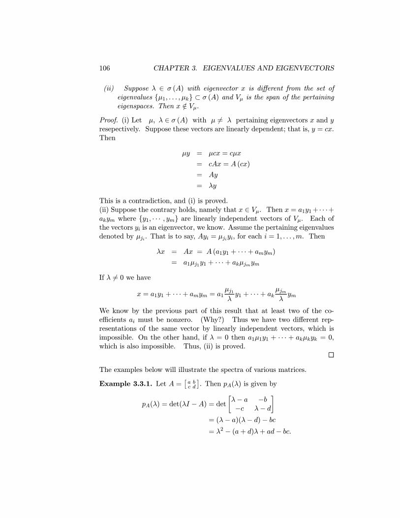
(ii) Suppose λ ∈ σ (A) with eigenvector x is different from the set ofeigenvalues {µ1, . . . , µk} ⊂ σ (A) and Vµ is the span of the pertainingeigenspaces. Then x /∈ Vµ.

Proof. (i) Let µ, λ ∈ σ (A) with µ = λ pertaining eigenvectors x and yresepectively. Suppose these vectors are linearly dependent; that is, y = cx.Then

µy = µcx = cµx

= cAx = A (cx)

= Ay

= λy

This is a contradiction, and (i) is proved.(ii) Suppose the contrary holds, namely that x ∈ Vµ. Then x = a1y1+ · · ·+akym where {y1, · · · , ym} are linearly independent vectors of Vµ. Each ofthe vectors yi is an eigenvector, we know. Assume the pertaining eigenvaluesdenoted by µji . That is to say, Ayi = µjiyi, for each i = 1, . . . ,m. Then

λx = Ax = A (a1y1 + · · ·+ amym)= a1µj1y1 + · · ·+ akµjmym

If λ = 0 we have

x = a1y1 + · · ·+ amym = a1µj1λy1 + · · ·+ akµjm

λym

We know by the previous part of this result that at least two of the co-efficients ai must be nonzero. (Why?) Thus we have two different rep-resentations of the same vector by linearly independent vectors, which isimpossible. On the other hand, if λ = 0 then a1µ1y1 + · · · + akµkyk = 0,which is also impossible. Thus, (ii) is proved.

The examples below will illustrate the spectra of various matrices.

Example 3.3.1. Let A = a bc d . Then pA(λ) is given by

pA(λ) = det(λI −A) = det λ− a −b−c λ− d

= (λ− a)(λ− d)− bc= λ2 − (a+ d)λ+ ad− bc.


The eigenvalues are the roots of pA(λ) = 0

λ =a+ d± (a+ d)2 − 4(ad− bc)

2

=a+ d± (a− d)2 + 4bc

2.

For this quadratic there are three possibilities:

(a) Two real rootsdifferent values

equal values

(b) Two complex roots

Here are three 2 × 2 examples that illustrate each possibility. The readershould compute the characteristic polynomials to verify these computation.

B1 =1 −11 −1 . Then pB1(λ) = λ2 λ = 0, 0

B2 =0 −11 0

. Then pB2(λ) = λ2 + 1 λ = ±i

B3 =0 11 0

. Then pB3(λ) = λ2 − 1 λ = ±1.

Example 3.3.2. Consider the rotation in the x, z-plane through an angleθ

B =

cos θ 0 − sin θ0 1 0sin θ 0 cos θ

The characteristic polynomial is given by

pB (λ) = det

λ 1 0 00 1 00 0 1

− cos θ 0 − sin θ

0 1 0sin θ 0 cos θ

= −1 + (1 + 2 cos θ)λ− (1 + 2 cos θ)λ2 + λ3

The eigenvalues are 1, cos θ +√cos2 θ − 1, cos θ − √cos2 θ − 1. When θ

is not equal to an even multiple of π, exactly two of the roots are complexnumbers. In fact, they are complex conjugate pairs, which can also bewritten as cos θ + i sin θ, cos θ − i sin θ. The magnitude of each eigenvalue


is 1, which means all three eigenvalues lie on the unit circle in the complexplane. An interesting observation is that the characteristic polynomial andhence the eigenvalues are the same regardless of which pair of axes (x-z,x-y, or y-z) is selected for the rotation. Matrices of the form B are actuallycalled rotations. In two dimensions the counter-clockwise rotations throughthe angle θ are given by

Bθ =cos θ − sin θsin θ cos θ

The eigenvalues for all θ is not equal to an even multiple of π are ±i. (SeeExercise 2.)

Example 3.3.3. If T is upper triangular with diag T = [t11, t22, . . . , tnn].Then λI−T is upper triangular with diag[λ− t11,λ− t22, . . . ,λ− tnn]. Thusthe determinant of λI − T gives the characteristic polynomial of T to be

pT (λ) =n

i=1

(λ− tii)

The eigenvalues of T are the diagonal elements of T . By expanding thisproduct we see that

pT (λ) = λn − (Σtii)λn−1 + lower order terms.

The constant term of pT (λ) is (−1)nn

i=1tii = (−1)n detT . We define

tr T =n

i=1

tii

and call it the trace of T . The same statements apply to lower triangularmatrices. Moreover, the trace definition applies to all matrices, not just totriangular ones, and the result will be the same.

Example 3.3.4. Suppose that A is rank 1. Then there are two vectorsw, z ∈ Cn for which

A = wzT .

To find the spectrum of A we consider the equation

Ax = λx


or

z, x w = λx.

From this we see that x = w is an eigenvector with eigenvalue z, w . Ifz⊥x, x is an eigenvector pertaining to the eigenvalue 0. Therefore,

σA = { z, w , 0}.The characteristic polynomial is

pλ(λ) = (λ− z, w )λn−1.

If w and z are orthogonal then

pA(λ) = λn.

If w and z are not orthogonal though there are just two eigenvalues, we saythat 0 is an eigenvalue of multiplicity n− 1, the order of the factor (λ− 0).Also z, w has multiplicity 1. This is the subject of the next section.

For instance, suppose w = (1,−1, 2) and z = (0, 1,−3). Then spectrumof the matrix A = wzT is given by σ(A) = {−7, 0}. The eigenvalue pertain-ing to λ = −7 is w and we may take x = (0, 3, 1) and (c, 3, 1), for any c ∈ C,to be eigenvectors pertaining to λ = 0. Note that {w, (0, 3, 1), (1, 3, 1)} forma basis for R3.

To complete our discussion of characteristic polynomials we prove a re-sult that every nth degree polynomial with lead coefficient one is the char-acteristic polynomial of some matrix. You will note the similarity of thisresult and the analogous result for differential systems.

Theorem 3.3.3. Every polynomial of nth degree with lead coefficient 1, thatis

q (λ) = λn + b1λn−1 + · · ·+ bn−1λ+ bn

is the characteristic polynomial of some matrix.

Proof. We consider the n× n matrix

B =

0 1 0 · · · 00 0 1 0...

. . .

−bn −bn−1 −b1


Then λI −B has the form

λI −B =

λ −1 0 · · · 00 λ −1 0... λ

. . .

bn bn−1 λ+ b1

Now expand in minors across the bottom row to get

det (λI −B) = bn (−1)n+1 det

−1 0 · · · 0λ −1 0

λ. . .

+bn−1 (−1)n+2 det

λ 0 · · · 00 −1 0... λ

. . .

+ · · ·+b1 (−1)n+n det

λ −1 0 · · ·0 λ −1... λ

. . .

= bn (−1)n+1 (−1)n−1 + bn−1 (−1)n+2 λ (−1)n−2 + · · ·

+(λ+ b1) (−1)n+n λn−1= bn + bn−1λ+ · · ·+ b1λn−1 + λn

which is what we set out to prove. (The reader should check carefully theterm with bn−2 to fully understand the nature of this proof.)

Multiplicity

Let A ∈ Mn(C). Since pA(λ) is a polynomial of degree exactly n, it musthave exactly n eigenvectors (i.e. roots) λ1,λ2, . . . ,λn counted according tomultiplicity. Recall that the multiplicity of an eigenvalue is the number oftimes the monomial (λ − λi) is repeated in the factorization of pA(λ). Forexample the multiplicity of the root 2 in the polynomial (λ − 2)3(λ − 5)is 3. Suppose µ1, . . . , µk are the distinct eigenvalues with multiplicitiesm1,m2, . . . ,mk respectively. Then the characteristic polynomial can be


rewritten as

pA(λ) = det(λI −A) =n

1

(λ− λi)

=k

1

(λ− µi)mi .

More precisely, the multiplicities m1,m2, . . . ,mk are called the algebraicmultiplicities of the respective eigenvalues. This factorization will be veryuseful later.

We know that for each eigenvalue λ of any multiplicity m, there mustbe at least one eigenvector pertaining to λ. What is desired, but not alwayspossible, is to find µ linearly independent eigenvectors corresponding to theeigenvalue λ of multiplicity m. This state of affairs makes matrix theory atonce much more challenging but also much more interesting.

Example 3.3.3. For the matrix

A =

2 0 0

0 74

14

√3

0 14

√3 5

4

the characteristic polynomial is det(λI − A) = pA (λ) = λ3 − 5λ2 + 8λ −4, which can be factored as pA (λ) = (λ− 1) (λ− 2)2 We see that theeigenvalues are 1, 2, and 2. So, the multiplicity of the eigenvalue λ = 1is 1, and the multiplicity of the eigenvalue λ = 2 is 2. The eigenspace

pertaining to the eigenvalue λ = 1 is generated by the vector

0

−13√3

1

,and the dimension of this eigenspace is one. The eigenspace pertaining to

λ = 2 is generated by

100

and 0

113

√3

. (That is, these two vectors forma basis of the eigenspace.) To summarize, for the given matrix there is oneeigenvector for the eigenvalue λ = 1, and there are two linearly independenteigenvectors for the eigenvalue λ = 2. The dimension of the eigenspacepertaining to λ = 1 is one, and the dimension of the eigenspace pertainingto λ = 2 is two.

Now contrast the above example where the eigenvectors span the space C3and the next example where we have an eigenvalue of multiplicity three butthe eigenspace is of dimension one.


Example 3.3.4. Consider the matrix

A =

2 −1 00 2 01 0 2

The characteristic polynomial is given by (λ− 2)3 . Hence the eigenvalueλ = 2 has multiplicity three. The eigenspace pertaining to λ = 2 is gener-ated by the single vector [0, 0, 1]T To see this we solve

(A− 2I)x =

2 −1 00 2 01 0 2

− 2 1 0 00 1 00 0 1

x=

0 −1 00 0 01 0 0

x = 0

The row reduced echelon form for

0 −1 00 0 01 0 0

is 1 0 00 1 00 0 0

. From

this it is apparent that we may take x3 = t, but that x1 = x2 = 0. Nowassign t = 1 to obtain the generating vector [0, 0, 1]T . This type of exampleand its consequences seriously complexifies the study of matrices.

Symmetric Functions

Definition 3.3.5. Let n be a positive integer and Λ = {λ1,λ2, . . . ,λn} begiven numbers. Suppose that k is a positive integer with 1 ≤ k ≤ n. Thekth elementary symmetric function on the Λ is defined by

Sk(λ1, . . . ,λn) =1≤i1<···<ik≤n

k

j=1

λij .

It is easy to see that

S1(λ1, . . . ,λn) =n

1

λi

Sn(λ1, . . . ,λn) =n

1

λi.


For a given matrix A ∈Mn there are n symmetric functions defined withrespect to its eigenvalues Λ = {λ1,λ2, . . . ,λn}. The symmetric functionsare sometimes called the invariants of matrices as they are invariant undersimilarity transformations that will be in Section 3.5. They also furnishdirectly the coefficients of the characteristic polynomial. Thus specifyingthe n symmetric functions of an n × n matrix is sufficient to determine itseigenvalues.

Theorem 3.3.4. Let A ∈Mn have symmetric functions Sk, k = 1, 2, . . . , n.Then

det(λI −A) =n

i=1

(λ− λi) = λn +n

k=1

(−1)kSkλn−k.

Proof. The proof is a consequence of actually expanding the product ni=1(λ−

λi). Each term in the expansion has exactly n terms multiplied together thatare combinations of the factor λ and the −λis. For example, for the powerλn−k the coefficient is obtained by computing the total number of productsof k “different” −1λis. (The term different is in quotes because it refersto different indices not actual values.) Collecting all these terms is accom-plished by addition. Now the number of ways we can obtain products ofthese k different (−1)λis is easily seen to be the number of sequences in theset {1 ≤ i1 < · · · < ik ≤ n}. The sum of these is clearly (−1)kSk, with the(−1)k factor being the collected product of k −1’s.

Two of the symmetric functions are familiar. In the following we restatethis using familiar terms.

Theorem 3.3.5. Let A ∈Mn(C). Then


k=0

pkλn−k

where p0 = 1 and

(i) p1 = −tr(A) = −n

1

aii

(ii) pn = −detA.(iii) pk = (−1)kSk, for 1 < k < n.


Proof. Note that pA(0) = −det(A) = pn. This gives (ii). To establish (i),we consider

det

λ · a11 −a12 . . . −a1n−a21 λ− a22 −a2n...

. . .

−an1 . . . λ− ann

.

Clearly the productn

1(λ − aii) is one of the selections of products in

the calculation process. In every other product there must be no more thann− 2 diagonal terms. Hence


1

(λ− aii) + pn−2(λ),

where pn−2(λ) is a polynomial of degree n − 2. The coefficient of λn−1 is−

n

1aii by the Theorem 3.3.4, and this is (i).

As a final note, observe that the characteristic polynomial is defined byknowing the n symmetric functions. However, the matrix itself has n2 en-tries. Therefore, one may expect that knowing the only characteristic poly-nomial of a matrix is insufficient to characterize it. This is correct. Manymatrices having rather different properties can have the same characteristicpolynomial.

3.4 The Hamilton-Cayley Theorem

The Hamilton-Cayley Theorem opens the doors to a finer analysis of a ma-trix through the use of polynomials, which in turn is an important tool ofspectral analysis. The results states that any square matrix satisfies its owncharactertic polynomial, that is pA(A) = 0. The proof is not difficult, but weneed some preliminary results about factoring matrix-valued polynomials.Preceding that we need to consider matrix polynomials in some detail.

Matrix polynomials

One of the very important results of matrix theory is the Hamilton-Cayleytheorem which states that a matrix satisfies its only characteristic equation.This implies we need the notion of a matrix polynomial. It is an easy idea

3.4. THE HAMILTON-CAYLEY THEOREM 115

– just replace the coefficients of any polynomial by matrices – but it bearssome important consequences.

Definition 3.4.1. Let A0, A1, . . . , Am be square n × n matrices. We candefine the polynomial with matrix coefficients

A(λ) = A0λm +A1λ

m−1 + · · ·+Am−1λ+Am.The degree of A(λ) is m, provided A0 = 0. A(λ) is called regular if detA0 =0. In this case we can construct an equivalent monic2 polynomial.

A(λ) = A−10 A(λ) = A−10 A0λ

m +A−10 A1λm−1 + · · ·+A−10 Am

= Iλm + A1λm−1 + · · ·+ Am.

The algebra of matrix polynomials mimics the normal polynomial algebra.Let

A(λ) =m

0

Aiλm−k B(λ) =

m

0

Biλm−k.

(1) Addition:

A(λ)±B(λ) =m

0

(Ak ±Bk)λm−k.

(2) Multiplication:

A(λ)B(λ) =m

i=0

λmm

k=0

AiBm−i

The term mk=0AiBm−i is called the Cauchy product of the sequences.

Note that the matrices Aj always multiply on the left of the Bk.

(3) Division: Let A(λ) and B(λ) be two matrix polynomials of degreem (as above) and suppose B(λ) is regular, i.e. detB0 = 0. We saythat Qr(λ) and Rr(λ) are right quotient and remainder of A(λ) upondivision by B(λ) if

A(λ) = Qr(λ)B(λ) +Rr(λ) (1)

2Recall that a monic polynomial is a polynomial where coefficient of the highest poweris one. For matrix polynomials the corresponding coefficient is I, the identity matrix.


if the degree of Rr(λ) is less than that of B(λ). Similarly Q (λ) andR (λ) are respectively the left quotient and remainder of A(λ) upondivision by B(λ) if

A(λ) = B(λ)Q (λ) +R (λ) (2)

if the degree of R (λ) is less than that of B(λ).

In the case (1) we see

A(λ)B−1(λ) = Qr(λ) +Rr(λ)B−1(λ), (3)

which looks much like ab = q+rb , a way to write the quotient and remainder

of a divided by b when a and b are numbers. Also, the form (3) may notproperly exist for all λ.

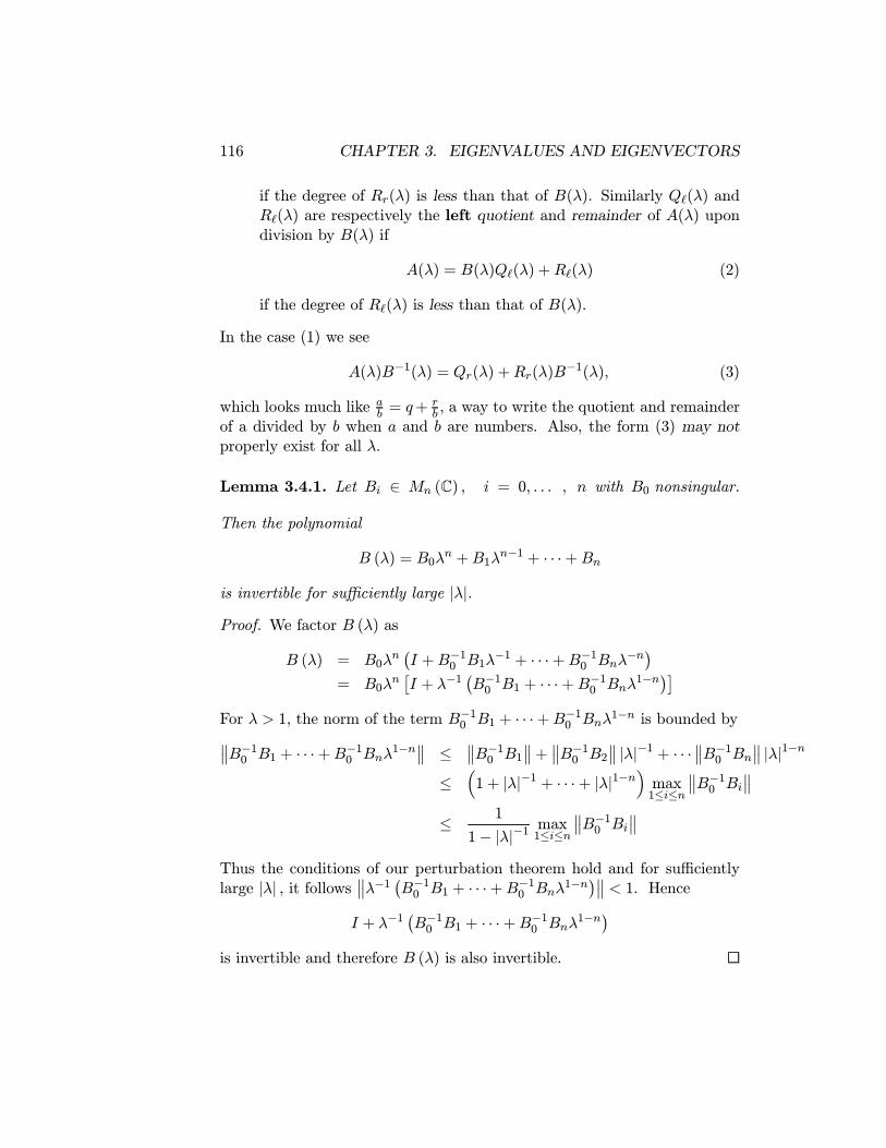
Lemma 3.4.1. Let Bi ∈ Mn (C) , i = 0, . . . , n with B0 nonsingular.

Then the polynomial

B (λ) = B0λn +B1λ

n−1 + · · ·+Bnis invertible for sufficiently large |λ|.Proof. We factor B (λ) as

B (λ) = B0λn I +B−10 B1λ

−1 + · · ·+B−10 Bnλ−n

= B0λn I + λ−1 B−10 B1 + · · ·+B−10 Bnλ

1−n

For λ > 1, the norm of the term B−10 B1 + · · ·+B−10 Bnλ1−n is bounded by

B−10 B1 + · · ·+B−10 Bnλ1−n ≤ B−10 B1 + B−10 B2 |λ|−1 + · · · B−10 Bn |λ|1−n

≤ 1 + |λ|−1 + · · ·+ |λ|1−n max1≤i≤n

B−10 Bi

≤ 1

1− |λ|−1 max1≤i≤nB−10 Bi

Thus the conditions of our perturbation theorem hold and for sufficientlylarge |λ| , it follows λ−1 B−10 B1 + · · ·+B−10 Bnλ

1−n < 1. Hence

I + λ−1 B−10 B1 + · · ·+B−10 Bnλ1−n

is invertible and therefore B (λ) is also invertible.


Theorem 3.4.1. Let A(λ) and B(λ) be matrix polynomials in Mn(C) or(Mn(R)). Then both left and right division of A(λ) by B(λ) is possible andthe respective quotients and remainders are unique.

Proof. We proceed by induction on degB, and clearly if degB = 0 the resultholds. If degB = p > degA(λ) = m then the result follows simply. For,take Qr(λ) = 0 and Rr(λ) = A(λ). The conditions of right division are met.Now suppose that p ≤ m. It is easy to see that

A(λ) = A0λm +A1λ

m−1 + · · ·+Am−1λ+Am

= A0B−10 λm−pB(λ)−

p

j=1

A0B−10 Bjλ

m−j +m

j=1

Ajλm−j

= Q1(λ)B(λ) +A1(λ)

where degA1(λ) < degA(λ). Our inductive hypothesis assumed the divisionwas possible for matrix polynomials A(λ) of degree < p. Therefore, A1(λ) =Q2(λ)B() + R(λ), where the degree of B(λ) < p. Finally, with Q(λ) =Q(λ) +Q2(λ), there results A(λ) = Q(λ)B() +R(λ).

To establish uniqueness we assume two right divisors and quotients havebeen determined. Thus

A = Qr1(λ)B(λ) +Rr1(λ)

A = Qr2(λ)B(λ) +Rr2(λ)

Subtract to get

0 = (Qr1(λ)−Qr2(λ))B(λ) +Rr1(λ)−Rr2(λ).If Qr1(λ) − Qr2(λ) = 0, we know the degree of (Qr1(λ) − Qr2(λ))B(λ) isgreater than the degree of R1(λ) − R2(λ). This contradiction implies thatQr1(λ)−Qr2(λ) = 0, which in turn implies that Rr1(λ)−Rr2(λ) = 0. Hencethe decomposition is unique.

Hamilton-Cayley Theorem

Let

B(λ) = B0λm +B1λ

m−1 + · · ·+Bm−1λ+Bm

with B0 = 0. We can also, write B(λ) =m

i=0λm−iBi. Both versions are

the same. However, when A ∈Mn(F ), there are two possible evaluations ofB(A).


Definition 3.4.2. Let B(λ), A ∈ Mn(C) (or Mn(R)) and B(λ) = B0λm +

B1λm−1 + · · ·+Bm−1λ+Bm. Define

B(A) = B0Am +B1A

m−1 + · · ·+Bm “right value”

B(A) = AmB0 +Am−1B1 + · · ·+Bm “left value”

The generalized Bezout theorem gives the remainder of B(λ) divided byλI −A. In fact, we haveTheorem 3.4.2 (Generalized Bezout Theorem). The right division ofB(λ) by λI −A has remainder

Rr(λ) = B(A)

Similarly, the left division of B(λ) by (λI −A) has remainderR (λ) = B(A).

Proof. In the case degB(λ) = 1, we have

B0λ+B1 = B0(λI −A) +B0A+B1.The remainder Rr(λ) = B0A+B1 = B(A). Assume the result holds for allpolynomials up to degree p− 1. We have

B(λ) = B0λp +B1λ

p−1 + · · ·+Bp= B0λ

p−1(λI −A) +B0Aλp−1 +B1λp−1 + · · ·= B0λ

p−1(λI −A) +B1(λ)where degB1(λ) ≤ p− 1. By induction

B(λ) = B0λp−1(λI −A) +Qr(λ)(λI −A) +B1(A)

B1(A) = (B0A + B1)Ap−1 + B2Ap−2 + · · · + Bp−1A + Bp = B(A). This

proves the result.

Corollary 3.4.1. (λI − A) divides B(λ) if and only if B(A) = 0 (respB(A) = 0).

Combining the Bezout result and the adjoint formulation of the matrixinverse, we can establish the important Hamilton-Cayley theorem.

Theorem 3.4.3 (Hamilton-Cayley). Let A ∈ Mn(C) (or Mn(R)) withcharacteristic polynomial pA(λ). Then pA(A) = 0.


Proof. Recall the adjoint formulation of the inverse as C = 1det ·CC

Tij = C

−1.Now let B = adj(A− λI). Then

B(λI −A) = det(λI −A)I(λI −A)B = det(λI −A)I.

These equations show that p(λ)I = det(λI − A)I is divisible on the rightand the left by (λI −A) without remainder. It follows from the generalizedBezout theorem that this is possible only if pA(A) = 0.

Let A ∈ Mn (C) . Now that we know any A satisfies its characteristicpolynomial, we might also ask if there are polynomials of lower degree that italso satisfies. In particular, we will study the so-called minimal polynomialthat a matrix satisfies. The nature of this polynomial will shed considerablelight on the fundamental structure of A. For example, both matrices belowhave the same characteristic polynomial P (λ) = (λ− 2)3.

A =

2 0 00 2 00 0 2

and B = 2 1 00 2 10 0 2

Hence λ = 2 is an eigenvalue of multiplicity three. However, A satifies themuch simpler first degree polynomial (λ− 2) while there is no polynomialof degree less that three that B satisfies. By this time you recognizethat A has three linearly independent eigenvectors, while B has only oneeigenvector. We will take this subject up in a later chapter.

Biographies

Arthur Cayley (1821-1895), one of the most prolific mathematicians of hisera and of all time, born in Richmond, Surrey, and studied mathematics atCambridge. For four years he taught at Cambridge having won a Fellowshipand, during this period, he published 28 papers in the Cambridge Mathe-matical Journal. A Cambridge fellowship had a limited tenure so Cayleyhad to find a profession. He chose law and was admitted to the bar in 1849.He spent 14 years as a lawyer, but Cayley always considered it as a meansto make money so that he could pursue mathematics. During these 14 yearsas a lawyer Cayley published about 250 mathematical papers! Part of thattime he worked in collaboration with James Joseph Sylvester3 (1814-

3In 1841 he went to the United States to become professor at the University of Virginia,but just four years later resigned and returned to England. He took to teaching private


1897), another lawyer. Together, but not in collaboration, they founded thealgebraic theory of invariants 1843.

In 1863 Cayley was appointed Sadleirian professor of Pure Mathemat-ics at Cambridge. This involved a very large decrease in income. HoweverCayley was very happy to devote himself entirely to mathematics. He pub-lished over 900 papers and notes covering nearly every aspect of modernmathematics.

The most important of his work is in developing the algebra of matrices,work in non-Euclidean geometry and n-dimensional geometry. Importantly,he also clarified many of the theorems of algebraic geometry that had previ-ously been only hinted at, and he was among the first to realize how manydifferent areas of mathematics were linked together by group theory.

As early as 1849 Cayley wrote a paper linking his ideas on permutationswith Cauchy’s. In 1854 Cayley wrote two papers which are remarkable forthe insight they have of abstract groups. At that time the only knowngroups were groups of permutations and even this was a radically new area,yet Cayley defines an abstract group and gives a table to display the groupmultiplication.

Cayley developed the theory of algebraic invariance, and his develop-ment of n-dimensional geometry has been applied in physics to the studyof the space-time continuum. His work on matrices served as a founda-tion for quantum mechanics, which was developed by Werner Heisenberg in1925. Cayley also suggested that Euclidean and non-Euclidean geometryare special types of geometry. He united projective geometry and metricalgeometry which is dependent on sizes of angles and lengths of lines.

Heinrich Weber (1842-1913) was born and educated in Heidelberg, wherehe became professor 1869. He then taught at a number of institutions inGermany and Switzerland. His main work was in algebra and number theory.He is best known for his outstanding text Lehrbuch der Algebra publishedin 1895.

Weber worked hard to connect the various theories even fundamentalconcepts such as a field and a group, which were seen as tools and notproperly developed as theories in his Die partiellen Differentialgleichungender mathematischen Physik 1900-01, which was essentially a reworking of abook of the same title based on lectures given by Bernhard Riemann and

pupils and had among them Florence Nightingale. By 1850 he became a barrister, and by1855 returned to an academic life at the Royal Military Academy in Woolwich, London. Hereturned to the US again in 1877 to become professor at the new Johns Hopkins University,but returned to England once again in 1877. Sylvester coined the term ‘matrix’ in 1850.


written by Karl Hattendorff.

Etienne Bezout (1730-1783) was a mathematician who represents a char-acteristic aspect of the subject at that time. One of the many successfultextbook projects produced in the 18th century was Bezout’s Cours de math-ematique, a six volume work that first appeared in 1764-1769, which wasalmost immediately issued in a new edition of 1770-1772, and which boastedmany versions in French and other languages. (The first American textbookin analytic geometry, incidentally, was derived in 1826 from Bezout’s Cours.)

It was through such compilations, rather than through the original worksof the authors themselves, that the mathematical advances of Euler andd’Alembert became widely known. Bezout’s name is familiar today in con-nection with the use of determinants in algebraic elimination. In a memoirof the Paris Academy for 1764, and more extensively in a treatise of 1779entitled Theorie generale des equations algebriques, Bezout gave artificialrules, similar to Cramer’s, for solving n simultaneous linear equations in nunknowns. He is best known for an extension of these to a system of equa-tions in one or more unknowns in which it is required to find the conditionon the coefficients necessary for the equations to have a common solution.To take a very simple case, one might ask for the condition that the equa-tions a1x + b1y + c1 = 0, a2x + b2y + c2 = 0, a3x + bay + c3 = 0 have acommon solution. The necessary condition is that the eliminant a specialcase of the “Bezoutiant,” should be 0.

Somewhat more complicated eliminants arise when conditions are soughtfor two polynomial equations of unequal degree to have a common solution.Bezout also was the first one to give a satisfactory proof of the theorem,known to Maclaurin and Cramer, that two algebraic curves of degreesm andn respectively intersect in general in m · n points; hence, this is often calledBezout’s theorem. Euler also had contributed to the theory of elimination,but less extensively than did Bezout.

Taken from A History of Mathematics by Carl Boyer


William Rowen HamiltonBorn Aug. 3/4, 1805, Dublin, Ire. and died Sept. 2, 1865, Dublin

Irish mathematician and astronomer who developed the theory of quater-nions, a landmark in the development of algebra, and discovered the phe-nomenon of conical refraction. His unification of dynamics and optics, more-over, has had lasting influence on mathematical physics, even though thefull significance of his work was not fully appreciated until after the rise ofquantum mechanics.

Like his English contemporaries Thomas Babington Macaulay and JohnStuart Mill, Hamilton showed unusual intellect as a child. Before the ageof three his parents sent him to live with his father’s brother, James, alearned clergyman and schoolmaster at an Anglican school at Trim, a smalltown near Dublin, where he remained until 1823, when he entered TrinityCollege, Dublin. Within a few months of his arrival at his uncle’s he couldread English easily and was advanced in arithmetic; at five he could translateLatin, Greek, and Hebrew and recite Homer, Milton and Dryden. Beforehis 12th birthday he had compiled a grammar of Syriac, and by the age of14 he had sufficient mastery of the Persian language to compose a welcometo the Persian ambassador on his visit to Dublin.

Hamilton became interested in mathematics after a meeting in 1820with Zerah Colburn, an American who could calculate mentally with aston-ishing speed. Having read the Elements d’algebre of Alexis—Claude Clairautand Isaac Newton’s Principia, Hamilton had immersed himself in the fivevolumes of Pierre—Simon Laplace’s Traite de mecanique celeste (1798-1827;Celestial Mechanics) by the time he was 16. His detection of a flaw inLaplace’s reasoning brought him to the attention of John Brinkley, pro-fessor of astronomy at Trinity College. When Hamilton was 17, he sentBrinkley, then president of the Royal Irish Academy, an original memoirabout geometrical optics. Brinkley, in forwarding the memoir to the Acad-emy, is said to have remarked: “This young man, I do not say will be, butis, the first mathematician of his age.”

In 1823 Hamilton entered Trinity College, from which he obtained thehighest honours in both classics and mathematics. Meanwhile, he continuedhis research in optics and in April 1827 submitted this “theory of Systemsof Rays” to the Academy. The paper transformed geometrical optics intoa new mathematical science by establishing one uniform method for thesolution of all problems in that field. Hamilton started from the principle,originated by the 17th-century French mathematician Pierre de Fermat, thatlight takes the shortest possible time in going from one point to another,whether the path is straight or is bent by refraction. Hamilton’s key idea

3.5. SIMILARITY 123

was to consider the time (or a related quantity called the “action”) as afunction of the end points between which the light passes and to show thatthis quantity varied when the coordinates of the end points varied, accordingto a law that he called the law of varying action. He showed that the entiretheory of systems of rays is reducible to the study of this characteristicfunction.

Shortly after -Hamilton submitted his paper and while still an under-graduate, Trinity College elected him to the post of Andrews professor ofastronomy and royal astronomer of Ireland, to succeed Brinkley, who hadbeen made bishop. Thus an undergraduate (not quite 22 years old) becameex officio an examiner of graduates who were candidates for the Bishop LawPrize in mathematics. The electors’ object was to provide Hamilton witha research post free from heavy teaching duties. Accordingly, in October1827 Hamilton took up residence next to Dunsink Observatory, 5 miles (8km) from Dublin, where he lived for the rest of his life. He proved to be anunsuccessful observer, but large audiences were attracted by the distinctlyliterary flavour of his lectures on astronomy. Throughout his life Hamiltonwas attracted to literature and considered the poet William Wordsworthamong his fiends, although Wordsworth advised him to write mathematicsrather than poetry.

With eigenvalues we are able to begin spectral analysis. That part isthe derivation of the various normal forms for matrices. We begin with arelatively weak form of the Jordan form, which is coming up.

First of all, as you have seen diagonal matrices furnish the easiest formfor matrix analysis. Also, linear systems are very simple to solve for diagonalmatrices. The next simplest class of matrices are the triangular matrices.We begin with the following result based on the idea of similarity.

3.5 Similarity

Definition 3.5.1. A matrix B ∈ Mn is said to be similar to A ∈ Mn ifthere exists a nonsingular matrix S ∈Mn such that

B = S−1AS.

The transformation A→ S1AS is called a similarity transformation. Some-times we write A ∼ B. Note that similarity is an equivalence relation:

(i) A ∼ A reflexivity(ii) B ∼ A⇒ A ∼ B symmetry(iii) B ∼ A and A ∼ C ⇒ B ∼ C transitivity


Theorem 3.5.1. Similar matrices have the same characteristic polynomial.

Proof. We suppose A,B, and S ∈ Mn with S invertible and B = S−1AS.Then

λI −B = λI − S−1AS= λS−1IS − S−1AS= S−1(λI −A)S.

Hence

det(λI −B) = det(S−1(λI −A)S)= det(S−1) det(λI −A) detS= det(λI −A)

because 1 = det I = det(SS−1) = detS detS−1.

A simple consequence of Theorem 3.5.1 and Corollary 2.3.1 follows.

Corollary 3.5.1. If A and B are in Mn and if A and B are similar, thenthey have the same eigenvalues counted according to multiplicity, and there-fore the same rank.

We remark that even though [ 0 00 0 ] and [0 10 0 ] have the same eigenvalues,

0 and 0, they are not similar. Hence the converse is not true.

Another immediate corollary of Theorem 3.5.1 can be expressed in termsof the invariance of the trace and determinant of similarity transformations,that is functions on Mn(F ) defined for any invertible matrix S by TS(A) =S−1AS. Note that such transformations are linear mappings fromMn(F )→Mn(F ). We shall see how important are those properties of matrices thatare invariant (i.e. do not change) under similarity transformations.

Corollary 3.5.2. If A, B ∈Mn are similar, then they have the same traceand same determinant. That is, tr(A) = tr(B) and detA = detB.

Theorem 3.5.2. If A ∈Mn, then A is similar to a triangular matrix.

Proof. The following sketch shows the first two steps of the proof. A formalinduction can be applied to achieve the full result.

Let λ1 be an eigenvalue of A with eigenvector u1. Select a basis , sayS1, of Cn and arrange these vectors into columns of the matrix P1, with u1

3.5. SIMILARITY 125

in the first column. Define B1 = P−11 AP1. Then B1 is the representation of

A in the new basis and so

B1 =

λ α1 . . . αn−10... A20

where A2 is (n− 1)× (n− 1)

because Au1 = λ1u1. Remembering that B1 is the representation of A inthe basis S1, then [u1]S1 = e1 and hence B1e1 = λe1 = λ1[1, 0, . . . , 0]

T . Bysimilarity, the characteristic polynomial of B1 is the same as that of A, butmore importantly (using expansion by minors down the first column)

det(λI −B1) = (λ− λ1) det(λIn−1 −A2).Now select an eigenvalue λ2 of A2 and pertaining eigenvector v2 ∈ Cn; soA2v2 = λ2v2. Note that λ2 is also an eigenvalue of A. With this vector wedefine

u1 =

10...0

u2 =

0v2

.Select a basis of Cn−1, with v2 selected first and create the matrix P2 withthis basis as columns

P2 =

1 0 . . . 00... P20

.It is an easy matter to see that P2 is invertible and

B2 = P−12 B1P2

=

λ1 ∗ . . . . . . ∗0 λ2 ∗ . . . ∗0 0 A3...

...0 0

.Of course, B2 ∼ B1, and by the transitivity of similarity B2 ∼ A. Con-

tinue this process, deriving ultimately the triangular matrix Bn ∼ Bn−1 andhence Bn ∼ A. This completes the proof.


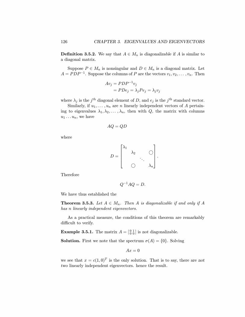
Definition 3.5.2. We say that A ∈Mn is diagonalizable if A is similar toa diagonal matrix.

Suppose P ∈ Mn is nonsingular and D ∈ Mn is a diagonal matrix. LetA = PDP−1. Suppose the columns of P are the vectors v1, v2, . . . , vn. Then

Avj = PDP−1vj

= PDej = λjPej = λjvj

where λj is the jth diagonal element of D, and ej is the j

th standard vector.Similarly, if u1, . . . , un are n linearly independent vectors of A pertain-

ing to eigenvalues λ1,λ2, . . . ,λn, then with Q, the matrix with columnsu1 . . . un, we have

AQ = QD

where

D =

λ1

λ2. . .

λn

.Therefore

Q−1AQ = D.

We have thus established the

Theorem 3.5.3. Let A ∈ Mn. Then A is diagonalizable if and only if Ahas n linearly independent eigenvectors.

As a practical measure, the conditions of this theorem are remarkablydifficult to verify.

Example 3.5.1. The matrix A = [ 0 10 0 ] is not diagonalizable.

Solution. First we note that the spectrum σ(A) = {0}. Solving

Ax = 0

we see that x = c(1, 0)T is the only solution. That is to say, there are nottwo linearly independent eigenvectors. hence the result.

3.5. SIMILARITY 127

Corollary 3.5.3. If A ∈ Mn is diagonalizable and B is similar to A, thenB is diagonalizable.

Proof. The proof follows directly from transitivity of similarity. However,more directly, suppose that B ∼ A and S is the invertible matrix such thatB = SAS−1 Then BS = SA. If u is an eigenvector of A with eigenvalue λ,then SAu = λSu and therefore BSu = λSu. This is valid for each eigenvec-tor. We see that if u1, . . . , un are the eigenvalues of A, then Su1, . . . , Sunare the eigenvalues of B. The similarity matrix converts the eigenvectors ofone matrix to the eigenvectors of the transformed matrix.

In light of these remarks, we see that similarity transforms preserve com-pletely the dimension of eigenspaces. It is just as significant to note thatif a similarity transformation diagonalizes a given matrix A, the similaritymatrix must consist of the eigenvectors of A.

Corollary 3.5.4. Let A ∈ Mn be nonzero and nilpotent. Then A is notdiagonalizable.

Proof. SupposeA ∼ T , where T is triangular. SinceA is nilpotent (i.e.(Am =0), T is nilpotent, as well. Therefore the diagonal entries of T are zero. Thespectrum of T and hence A is zero, it’s null space has dimension n. There-fore, by Theorem 2.3.3(f), its rank is zero. Therefore T = 0, and henceA = 0. The result is proved.

Alternatively, if the nilpotent matrix A is similar to a diagonal matrix withzero diagonal entries, then A is similar to the zero matrix. Thus A is itselfthe zero matrix. From the obvious fact that the power of a similarity trans-formations is the similarity transformation of the power of a matrix, that is(SAS−1)m = SAmS−1 (see Exercise 26), we have

Corollary 3.5.5. Suppose A ∈ Mn(C) is diagonalizable. (i) Then Am isdiagonalizable for every positive integer m. (ii) If p(·) is any polynomial,then p(A) is diagonalizable.

Corollary 3.5.6. If all the eigenvalues of A ∈Mn(C) are distinct, then Ais diagonalizable.

Proposition 3.5.1. Let A ∈Mn(C) and ε > 0. Then for any matrix norm· there is a matrix B with norm B < ε for which A+B is diagonalizableand for each λ ∈ σ(A) there is a µ ∈ σ(B) for which |λ− µ| < ε.


Proof. First triangularize A to T by a similarity transformation, T = SAS−1.Now add to T any diagonal matrix D so that the resulting triangular ma-trix T +D has all distinct values. Moreover this can be accomplished by adiagonal matrix of arbitrarily small norm for any matrix norm. Then wehave

S−1 (T +D)S = S−1TS + S−1DS= A+B

where B := S−1DS. Now by the submultiplicative property of matrix normsB ≤ S−1DS ≤ S−1 D S . Thus to obtain the estimate B < ε,it is sufficient to take D ≤

S−1 S, which is possible as established

above. Since the spectrum σ(A + B) of A + B has n distinct values, itfollows that A+B is diagonalizable.

There are many, many results on diagonalizable and non-diagonalizable ma-trices. Here is an interesting class of nondiagonalizable matrices we willencounter later.

Proposition 3.5.2. pro Every matrix of the form

A = λI +N

where N is nilpotent and is not zero is not diagonalizable.

An important subclass has the form:

A =

λ 1

λ 1λ 1

. . . 1λ

“Jordan block”.

Eigenvectors

Once an eigenvalue is determined, it is a relatively simple matter to find thepertaining eigenvectors. Just solve the homogeneous system (λI −A)x = 0.Eigenvectors have a more complex structure and their study merits ourattention.Facts

(1) σ(A) = σ(AT ) including mutliplicities.

3.5. SIMILARITY 129

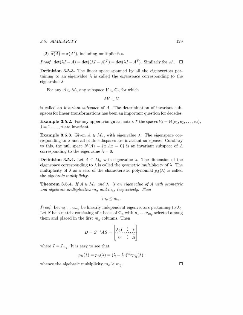
(2) σ(A) = σ(A∗), including multiplicities.

Proof. det(λI −A) = det((λI −A)T ) = det(λI −AT ). Similarly for A∗.Definition 3.5.3. The linear space spanned by all the eigenvectors per-taining to an eigenvalue λ is called the eigenspace corresponding to theeigenvalue λ.

For any A ∈Mn any subspace V ∈ Cn for whichAV ⊂ V

is called an invariant subspace of A. The determination of invariant sub-spaces for linear transformations has been an important question for decades.

Example 3.5.2. For any upper triangular matrix T the spaces Vj = S(e1, e2, . . . , ej),j = 1, . . . , n are invariant.

Example 3.5.3. Given A ∈ Mn, with eigenvalue λ. The eigenspace cor-responding to λ and all of its subspaces are invariant subspaces. Corollaryto this, the null space N(A) = {x|Ax = 0} is an invariant subspace of Acorresponding to the eigenvalue λ = 0.

Definition 3.5.4. Let A ∈ Mn with eigenvalue λ. The dimension of theeigenspace corresponding to λ is called the geometric multiplicity of λ. Themultiplicity of λ as a zero of the characteristic polynomial pA(λ) is calledthe algebraic multiplicity.

Theorem 3.5.4. If A ∈ Mn and λ0 is an eigenvalue of A with geometricand algebraic multiplicities mg and ma, respectively. Then

mg ≤ ma.Proof. Let u1 . . . umg be linearly independent eigenvectors pertaining to λ0.Let S be a matrix consisting of a basis of Cn with u1 . . . umg selected amongthem and placed in the first mg columns. Then

B = S−1AS =

λ0I ... ∗. . . . . . . . . . . .

0... B

where I = Img . It is easy to see that

pB(λ) = pA(λ) = (λ− λ0)mgpB(λ),

whence the algebraic multiplicity ma ≥ mg.


Example 3.5.4. For A = [ 0 10 0 ], the algebraic multiplicity of a is 2, whilethe geometric multiplicity of 0 is 1. Hence, the equality mg = ma is notpossible, in general.

Theorem 3.5.5. If A ∈ Mn and for each eigenvalue µ ∈ σ(A), mg(µ) =ma(µ), then A is diagonalizable. The converse is also true.

Proof. Extend the argument given in the theorem just above. Alternatively,we can see that A must have n linearly independent eigenvalues, whichfollows from the

Lemma 3.5.1. If A ∈ Mn and µ = λ are eigenvalues with eigenspaces Eµand Eλ respectively. Then Eµ and Eλ are linearly independent.

Proof. Suppose u ∈ Eµ can be expressed as

u =k

cjvj

where, of course u = 0 and vj = 0, j = 1, . . . , k where v1 . . . vk ∈ Eλ. ThenAu = AΣcjvj

⇒ µu = λΣcjvj

⇒ u =λ

µΣcjvj , if µ = 0.

Since λ/µ = 1, we have a contradiction. If µ = 0, then Σcjvj = 0 and thisimplies u = 0. In either case we have a contradiction, the result is thereforeproved.

While both A and AT have the same eigenvalues, counted even withmultiplicities, the eigenspaces can be very much different. Consider theexample where

A =1 10 2

and AT =1 01 2

.

The eigenvalue λ = 1 has eigenvector u = [ 10 ] for A and1−1 for AT .

A new concept of left eigenvector yield some interesting results.

Definition 3.5.5. We say λ is a left eigenvector of A ∈ Mn if there is avector y ∈ Cn for which

y∗A = λy∗

3.6. EQUIVALENT NORMS AND CONVERGENT MATRICES 131

or in Rn if yTA = λyT . Taking adjoints the two sides of this equality become

(y∗A)∗ = A∗y(λy∗)∗ = λy.

Putting these lines together A∗y = λy and hence λ is an eigenvalue of A∗.Here’s the big result.

Theorem 3.5.6. Let A ∈ Mn(C) with eigenvalues λ and eigenvector u.Let u, v be left eigenvectors pertaining to µ, λ, respectively. If µ = λ, v∗u =u, v = 0.

Proof. We have

v∗u =1

µv∗Aµ =

λ

µv∗u.

Assuming µ = 0 we have a contradiction. If µ = 0, argue as v∗u = 1λv∗Au =

µλc∗u = 0, which was to be proved. The result is proved.

Note that left eigenvectors of A are (right) eigenvectors of A∗ (AT in thereal case).

3.6 Equivalent norms and convergent matrices

Equivalent norms

So far we have defined a number of different norms. Just what “different”means is subject to different interpretations. For example, we might agreethat different means that the two norms have a different value for somematrix A. On the other hand if we have two matrix norms · a and · b,we might be prepared to say that if for two positive constants mM > 0

0 < m ≤ A a

A b≤M for all A ∈Mn(F )

then these norms are not really so different but rather are equivalent be-cause “small” in one norm implies “small” in the other and the same for“large.” Indeed, when two norms satisfy the condition above we will callthem equivalent. The remarkable fact is that all subordinate norms on afinite dimensional space are equivalent. This is a direct consequence of thesimilar result for vector norms. We state it below but leave the details ofthe proof to the reader.


Theorem 3.6.1. Any two matrix norms, · a and · b, on Mn(C) areequivalent in the sense that there exist two positive constants mM > 0

0 < m ≤ A a

A b≤M for all A ∈Mn(F )

We have already proved one convergence result about the invertibility ofI − A when A < 1. A deeper version of this result can be proved basedon a new matrix norm. This result has important consequences in generalmatrix theory and particularly in computational matrix theory. It is mostimportant in applications, where having ρ(A) < 1 can yield the same resultsas having A < 1.

Lemma 3.6.1. Let · be a matrix norm that is subordinate to the vectornorm (on Cn) · . Then for each A ∈Mn

ρ(A) ≤ A .

Note: We use the same notation for both vector and matrix norms.

Proof. Let λ ∈ σ(A). Then with corresponding eigenvector xλ we haveAxλ = λxλ. Normalizing xλ so that xλ = 1, we have A = max

x =1Ax ≥

Axλ = |λ| xλ = |λ|. Hence

A ≥ maxλ∈σ(A)

|λ| = ρ(A).

Theorem 3.6.2. For each A ∈ Mn and ε > 0 there is a vector norm ·on Cn for which the subordinate matrix norm · satisfies

ρ(A) ≤ A ≤ ρ(A) + ε.

Proof. The proof follows in a series of simple steps, the first of which isinteresting in its own right. First we know that A is similar to a triangularmatrix B–from a previous theorem

B = SAS−1 = Λ+ U

where Λ is the diagonal part of B and U is strictly upper triangular part ofB, with zeros filled in elsewhere.


Note that the diagonal of B is the spectrum of B and hence that of A.This is important. Now select a δ > 0 and form the diagonal matrix

D =

1

δ−1. . .

δ1−n

.A brief computation reveals that

C = DBD−1 = DSAS−1D−1

= D(Λ+ U)D−1

= Λ+DUD−1 = Λ+ V

where V = DUD−1 and more specifically vij = δj−iuij for j > i and ofcourse Λ is a diagonal matrix with the spectrum of A for the diagonal ele-ments. In this way we see that for δ small enough we have arranged thatA is similar to the diagonal matrix of its spectral elements plus a smalltriangular perturbation. We now define the new vector norm on Cn by

x A = (DS)∗(DS)x, x 1/2.

We recognise this to be a norm from a previous result. Now compute thematrix norm

A A = maxx A=1

Ax A.

Thus

Ax 2A = DSAx,DSAx

= CDSx,CDSx

≤ C 22 DSx

2

= C∗C 2 x2A.

From C = Λ+ V , it follows that

C∗C = Λ∗Λ+ Λ∗V + V ∗Λ+ V ∗V.

Because the last three terms have a δp multiplier for various positive powersp, we can make the terms Λ∗V + V ∗Λ+ V ∗V small in any norm by takingδ sufficiently small. Also the diagonal elements of Λ∗Λ have the form

|λi|2 λi ∈ S(A).


Talking δ sufficiently small so that each of Λ∗V 2, V∗Λ 2 and V ∗V 2 is

less than /3. With x 2A = 1 as required, we have

Ax A ≤ (ρ(A) + ε) x A

and we know already that A A ≥ ρ(A).

An important corollary places a lower bound on vector norms is givenbelow.

Corollary 3.6.1. For any A ∈Mn

ρ(A) = inf (maxx =1

Ax )

where the infimum is taken over all vector norms.

Convergent matrices

Definition 3.6.1. We say that a matrix A ∈ Mn(F ) for F = R or C isconvergent if

limm→∞A

m = 0 ← the zero matrix.

That is, for each 1 ≤ i, j ≤ n the limm→∞(Am)ij = 0. This is sometimescalled pointwise convergence.

Theorem 3.6.3. The following three statements are equivalent:

(a) A is convergent.

(b) limn→∞ Am = 0, for some matrix norm.

(c) ρ(A) < 1.

Proof. These results follow substantially from previously proven results.However, for completeness, assume (a) holds. Then

limn→∞maxij

|(An)ij | = 0

or what is the same we have

limn→∞ An ∞ = 0


which is (b). Now suppose that (b) holds. If ρ(A) ≥ 1 there is a vectorx for which Anx = ρ(A) n x . Therefore An ≥ 1, which contradicts(b). Thus (c) holds. Next if (c) holds we can apply the above theorem toestablish that there is a norm for which A < 1. Hence (b) follows. Finally,we know that

Am ∞ ≤M Am ( )

whence limn→∞A

m = 0. (That is (a) ≡ (b)). In sum we have shown that (a)

≡ (b) and (b) ≡ (c).

To establish ( ) we need the following.

Theorem 3.6.4. If and · are two vector norms on Cn then thereare constants m and M so that

m x ≤ x < M x

for all x ∈ Cn.

This result carries over to matrix norms subordinate to vector norms bysimple inheritance. To prove this result we use compactness ideas. Supposethere is a sequence of vectors xj for which

1 ≤ xj <1

jxj

and for which the components of xj are bounded in modulus. By compact-ness there is a convergent subsequence of the xj , for which limxj = x = 0.But x <∞. Hence x = 0, a contradiction.

Here is the new and improved version of our previous result.

Theorem 3.6.5. If ρ(A) < 1 then (I −A)−1 exists and

(I −A)−1 = I +A+A2 + · · · .

Proof. Select a matrix norm · for which A < 1. Apply previous calcu-lations. We know that every matrix can be triangularized and “almost” di-agonalized we may ask if we can eliminate altogether the off-diagonal terms.The answer is unfortunately no. But we can resolve the diagonal questioncompletely.


3.7 Exercises

1. Suppose that U ∈ Mn is orthogonal and let · be a matrix norm.Show that U ≥ 1.

2. In two dimensions the counter-clockwise rotations through the angleθ are given by

Bθ =cos θ − sin θsin θ cos θ

Find the eigenvalues and eigenvectors for all θ. (Note the two specialcases, θ is not equal to an even multiple of π and θ = 0.

3. Given two matrices A, B ∈ Mn (C). Define the commutant of A andB by [A,B]−AB −BA. Prove that tr[A,B] = 0.

4. Given two finite sequences {ck}nk=1 and {dk}nk=1. Prove that k |ckdk| ≤maxk |dk| k |ck|.

5. Verify that a matrix norm which is subordinate to a vector norm sat-isfies norm conditions (i) and (ii).

6. Let A ∈ Mn (C) . Show that the matrix norm subordinate to thevector norm · ∞ is given by

A ∞ = maxiri (A) 1

where as usual ri (A) denotes the ith row of the matrix A and · 1 is

the 1 norm.

7. The Hilbert matrix, Hn of order n is defined by

hij =1

i+ j − 1 1 ≤ i, j ≤ n

8. Show that Hn 1 < lnn.

9. Show that Hn ∞ = 1.

10. Show that Hn 2 ∼ n12 .

11. Show that the spectral radius of Hn is bounded by 1.

12. Show that for each ε > 0 there exists an integer N such that if n > Nthere is a vector x ∈ Rn with x 2=1 such that Hnx 2 < ε.

3.7. EXERCISES 137

13. Same as the previous question except that you need to show that

N = 1ε1/2

+ 1 will work.

14. Show that the matrix A =

1 1 00 3 11 −1 2

is not diagonalizable.LetA ∈Mn (C) .

15. We know that the characteristic polynomial of a matrix A ∈ M12 (C)is equal to pA (λ) = (λ− 1)12 − 1. Show that A is not similar to theidentity matrix.

16. We know that the spectrum of A ∈ M3 (C) is σ(A) = {1, 1,−2} andthe corresponding eigenvectors are {[1, 2, 1]T , [2, 1,−1]T , [1, 1, 2]T }.(i) Is it possible to determine A ? Why or why not? If so, prove it.

If not show two different matrices with the given spectrum andeigenvectors.

(ii) Is A diagonalizable?

17. Prove that if A ∈ Mn (C) is diagonalizable then for each λ ∈ σ (A) ,the algebraic and geometric multiplicities are equal. That is, ma (λ) =mg (λ) .

18. Show that B−1(λ) exists for |λ| sufficiently large.19. We say that a matrix A ∈ Mn (R) is row stochastic if all its entries

are non negative and the sum of the entries of each row is one.

(i) Prove that 1 ∈ σ (A) .(ii) Prove that ρ (A) = 1.

20. We say that A,B ∈Mn (C) are quasi -commutative if the spectrum ofAB −BA is just zero, i.e. σ (AB −BA) = {0}.

21. Prove that if AB is nilpotent then so is BA.

22. A matrix A ∈Mn (C) has a square root if there is a matrix B ∈Mn (C)such that B2 = A. Show that if A is diagonalizable then it has a squareroot.

23. Prove that every matrix that commutes with every diagonal matrix isitself diagonal.


24. Suppose that if A ∈Mn (C) is diagonalizable and for each λ ∈ σ (A) ,|λ| < 1. Prove directly from similarity ideas that limn→∞An =0.(That is, do not apply the more general theorem from the lecturenotes.)

25. We say that A is right quasi-invertible if there exists a matrix B ∈Mn (C) such that AB ∼ D, whereD is a diagonal matrix with diagonalentries nonzero. Similarly, we say that A is left quasi-invertible if thereexists a matrix B ∈Mn (C) such that BA ∼ D, where D is a diagonalmatrix with diagonal entries nonzero.

(i) Show that if A is right quasi-invertible then it is invertible.

(ii) Show that ifA is right quasi-invertible then it is left quasi-invertible.

(iii) Prove that quasi-invertibility is not an equivalence relation. (Hint.How do we usually show that an assertion is false?)

26. Suppose that A, S ∈Mn, with S invertible, andm is a positive integer.Show that (SAS−1)m = SAmS−1.

27. Consider the rotation 1 0 00 cos θ − sin θ0 sin θ cos θ

Show that the eigenvalues are the same as for the rotation cos θ 0 − sin θ

0 1 0sin θ 0 cos θ

See Example 2 of section 3.2.

28. Let A ∈Mn (C). Define eA = ∞n=0

An

n!. (i) Prove that exists. (ii)

Suppose that A, B ∈ Mn (C). Is eA+B = eAeB ? If not, when is ittrue?

29. Suppose that A, B ∈ Mn (C). We say A ` B if [A,B] = 0, where[·, ·] is the commutant. Prove or disprove that “`” is an equivalencerelation. Answer the same question in the case of quasi-commutivity.(See Exercise 20

30. Let u, v ∈ Cn. Find (I + uv∗)m.

3.8. APPENDIX A 139

31. Define the function f on Mm×n (C) by f(A) = rankA, and supposethat · is any matrix norm. Prove the following. (1) If for anymatrix A for which f(A) = n show that f is continuous in · . Thatis, for every ε > 0 then f(B) = n for every matrix B with BA < ε.is continuous in an ε-neighborhood of A. That is, for any B withA − B < ε, then f(B) = f(A). (This deviates slightly from theusual definition of continuity because the function f is integer valued.)(2) If f(A) < n, then f is not continuous in every ε-neighborhood ofA.

3.8 Appendix A

It is desired to solve the equation p (λ) = 0 for coefficients in p0, . . . , pn ∈ Cor R. The basic theorem on this subject is called the Fundamental Theo-rem of Algebra (FTA), whose importance is manifest by its hundreds ofapplications. Concommitant with the FTA is the notion of reducible andirreducible factors.

Theorem 3.8.1 (Theorem Fundamental Theorem of Algebra). Givenany polynomial p (λ) = p0λ

n+p1λn−1+· · ·+pn with coefficients in p0, . . . , pn ∈

C. There is at least one solution λ ∈ C to the equation p (λ) = 0.Though proving this result would take us too far afield of our subject,

we remarks that the simplest proof of this result no doubt comes as a di-rect application of Liouville’s Theorem, a result in complex analysis. As acorollary to the FTA, we have that there are exactly n solutions to p (λ) = 0when counted with multiplicitiy. Proved originally by Gauss, the proof ofthis theorem eluded mathematicians for many years. Let us assume thatp0 = 1 to make the factorization simpler to write. Thus

p (λ) =k

i=1

(λ− λi)mi (4)

.As we know, in the case that the coefficients p0, . . . , pn are real, there

may be complex solutions. As is easy to prove, complex solutions mustcome in complex conjugate pairs. For if λ = r + is is a solution

p (r + is) = (r + is)n + p1 (r + is)n−1 + · · · pn−1 (r + is) + pn = 0

Because the coefficients are real, the real and imaginary parts of the powers(r + is)j remain respectively real or imaginary upon multiplication by pj .


Thus

p (r + is) = Re (r + is)n + p1Re (r + is)n−1 + · · · pn−1Re (r + is) + pn

+i Im (r + is)n + p1Im (r + is)n−1 + · · · pn−1Im (r + is) + pn

= 0

Hence the real and imaginary parts are each zero. Since Re (r − is)j =Re (r + is)j and Im (r − is)j = −Im (r + is)j it follows that p (r − is) = 0.

In the case that the coefficients are real it may be of interest to notewhat statement of factorization analogous to (4) above. To this end weneed the definition

Definition 3.8.1. The real polynomial x2 + bx+ c is called irreducible ifit has no real zeros.

In general, any polynomial that cannot be factored over the underlyingfield is called irreducible. Irreducible polynomials have played a very impor-tant role in fields such as abstract algebra and number theory. Indeed, theywere central in early attempts to prove Fermat’s last theorem and also sobut more indirectly to the acutal proof. Our attention here is restricted tothe fields C and R.

Theorem 3.8.2. Let p (λ) = λn + p1λn−1 + · · · + pn with coefficients in

p0, . . . , pn ∈ R. Then p (λ) can be factored as a product of linear factorspertaining to real zeros of p (λ) = 0 and irreducible quadratic factors.

Proof. The proof is an easy application of the FTA and the observationabove. If λk = r+ is is a zero of p (λ), then so also is λk = r− is. Thereforethe product (λ− λk) λ− λk = λ2−2λr+r2+s2 is an irreducible quadratic.Combine such terms with the linear factors generated from the real zeros,and use (4).

Remark 3.8.1. It is worth noting that there are no higher order irreduciblefactors with real coefficients. Even though there are certainly higher orderpolynomials with complex roots, they can always factored as products ofeither real linear or real quadratic factors. Proving this without the FTAmay prove challenging.

3.9. APPENDIX B 141

3.9 Appendix B

3.9.1 Infinite Series

Definition 3.9.1. An infinite series, denoted by

a0 + a1 + a2 + · · ·

is a sequence {un}, where un is defined by

un = a0 + a1 + · · ·+ anIf the sequence {un} converges to some limit A, we say that the infiniteseries converges to A and use the notation

a0 + a1 + a2 + · · · = A

We also say that the sum of the infinite series is A. If {un} diverges, theinfinite series a0 + a1 + a2 + · · · is said to be divergent.

The sequence {un} is called the sequence of partial sums, and the se-quence {an} is called the sequence of terms of the infinite series a0 + a1 +a2 + · · · .

Let us now return to the formula

1 + r + r2 + · · ·+ rn = 1− rn+11− r

where r = 1. Since the sequence {rn+1} converges (and, in fact, to 0) if andonly if −1 < r < 1 (or |r| < 1), r being different from 1, the infinite series

1 + r + r2 + · · ·

converges to (1− r)−1 if and only if |r| < 1. This infinite series is called thegeometric series with ratio r.

Definition 3.9.2. Geometric Series with Ratio r

1 + r + r2 + · · · = 1

1− r , if |r| < 1

and diverges if |r| ≥ 1.Multiplying both sides by r yields the following.


Definition 3.9.3. If |r| < 1, thenr + r2 + r3 + · · · = r

1− rExample 3.9.1. Investigate the convergence of each of the following infi-nite series. If it converges, determine its limit (sum).a. 1− 1

2 +14 − 1

8 + · · · b. 1 + 23 +

49 +

827 + · · · c. 34 +

916 +

2764 + · · ·

Solution A careful study reveals that each infinite series is a geometricseries. In fact, the ratios are, respectively, (a) −12 , (b) 23 , and (c) 34 . Sincethey are all of absolute value less than 1, they all converge. In fact, we have:a. 1− 1

2 +14 − 1

8 + · · · = 11−(− 1

2)= 2

3

b. 1 + 23 +

49 +

827 + · · · = 1

1− 23

= 31 = 3

c. 34 +916 +

2764 + · · · =

34

1− 34

= 34 · 41 = 3

Since an infinite series is defined as a sequence of partial sums, the prop-erties of sequences carry over to infinite series. The following two propertiesare especially important.

1. Uniqueness of Limit If a0 + a1 + a2 + · · · converges, thenit converges to a unique limit.

This property explains the notation

a0 + a1 + a2 + · · · = Awhere A is the limit of the infinite series. Because of this notation, we oftensay that the infinite series sums to A, or the sum of the infinitely manyterms a0, a1, a2, . . . is A. We remark, however, that the order of the termscannot be changed arbitrarily in general.

Definition 3.9.4. 2. Sum of Infinite Series Ifa0 + a1 + a2 + · · · = A and b0 + b1 + b2 + · · · = B, then

(a0 + b0) + (a1 + b1) + (a2 + b2) + · · · = (a0 + a1 + a2 + · · · )+(b0 + b1 + b2 + · · · )

= A+B

This property follows from the observation that

(a0 + b0) + (a1 + b1) + · · ·+ (an + bn) = (a0 + a1 + · · ·+ an)+(b0 + b1 + · · ·+ bn)

converges to A+B. Another property is

3.9. APPENDIX B 143

Definition 3.9.5. 3. Constant Multiple of Infinite Series If a0+a1+a2 + · · · = A and c is a constant, then

ca0 + ca1 + ca2 + · · · = cAExample 3.9.2. Determine the sums of the following convergent infiniteseries.a. 5

3·2 +139·4 +

3527·8 + · · · b. 1

3·2 +19·2 +

127·2 + ·

Solution a. By the Sum Property, the sum of the first infinite series is

1

3+1

2+

1

9+1

4+

1

27+1

8+ · · ·

=1

3+1

9+1

27+ · · · +

1

2+1

4+1

8+ · · ·

=13

1− 13

+12

1− 12

=1

2+ 1 =

3

2

b. By the Constant-Multiple Property, the sum of the second infinite seriesis

1

2

1

3+1

9+1

27+ · · · =

1

2·

13

1− 13

=1

2· 12=1

4

Another type of infinite series can be illustrated by using Taylor poly-nomial extrapolation as follows.

Example 3.9.3. In extrapolating the value of ln 2, the nth-degree Taylorpolynomial Pn(x) of ln(1 + x) at x = 0 was evaluated at x = 1 in Example4 of Section 12.3. Interpret ln 2 as the sum of an infinite series whose nthpartial sum is Pn(1).

Solution We have seen in Example 3 of Section 12.3 that

Pn(x) = x− 12x2 +

1

3x3 − · · ·+ (−1)n−1 1

nxn

so that Pn(1) = 1− 12 +

13 − · · ·+(−1)n−1 1n , and it is the nth partial sum of

the infinite series

1− 12+1

3− 14+ · · ·

Since {Pn(1)} converges to ln 2 (see Example 4in Section 12.3), we have

ln 2 = 1− 12+1

3− 14− · · ·


It should be noted that the terms of the infinite series in the precedingexample alternate in sign. In general, an infinite series of this type alwaysconverges.

Alternating Series Test Let a0 ≥ a1 ≥ · · · ≥ 0. If an ap-proaches 0, then the infinite series

a0 − a1 + a2 − a3 + · · ·

converges to some limit A, where 0 < A < a0.

The condition that the term an tends to zero is essential in the aboveAlternating Series Test. In fact, if the terms do not tend to zero, the corre-sponding infinite series, alternating or not, must diverge.

Divergence Test If an does not approach zero as n → +∞,then the infinite series

a0 + a1 + a2 + · · ·

diverges.

Example 3.9.4. Determine the convergence or divergence of the followinginfinite series.

a. 1− 13 +

15 − 1

7 + · · · b. −23 + 45 − 6

7 + · · ·Solution a. This series is an alternating series with

1 >1

3>1

5> · · · > 0

and with the terms approaching 0. In fact, the general (nth) term is

(−1)n 1

2n+ 1

Hence, by the Alternating Series Test, the infinite series 1− 13 +

15 − 1

7 + · · ·converges.

b. Let a1 = −23 , a2 = 45 , a3 = −67 , . . . . It is clear that an does not approach

0, and it follows from the Divergence Test that the infinite series is divergent.[The nth term is (−1)n2n/(2n + 1).] Note, however, that the terms doalternate in sign.

3.9. APPENDIX B 145

Another useful tool for testing convergence or divergence of an infiniteseries is the Ratio Test, to be discussed below. Recall that the geometricseries

1 + r + r2 + · · ·where the nth term is an = r

n, converges if |r| < 1 and diverges otherwise.Note also that the ratio of two consecutive terms is

an+1an

=rn+1

rn= r

Hence, the geometric series converges if and only if this ratio is of absolutevalue less than 1. In general, it is possible to draw a similar conclusion if thesequence of the absolute values of the ratios of consecutive terms converges.

Ratio Test Suppose that the sequence

{|an+1|/|an|}converges to some limit R. Then, the infinite series a0 + a1 +a2 + · · · converges if R < 1 and diverges if R > 1.

Example 3.9.5. In each of the following, determine all values of r for whichthe infinite series converges.a. 1 + r + r2

2! +r3

3! + · · · b. 1 + 2r + 3r3 + 4r3 + · · ·Solution a. The nth term is an = r

n/n!, so that

an+1an

=rn+1

(n+ 1)!· n!rn=

r

n+ 1

For each value of r, we have

|an+1||an| =

1

n+ 1|r|→ 0 < 1

Hence, by the Ratio Test, the infinite series converges for all values of r.b. Let an = (n+ 1)r

n. Then,

|an+1||an| =

(n+ 2)|r|n+1(n+ 1)|r|n =

n+ 2

n+ 1|r|→ |r|

Hence, the Ratio Test says that the infinite series converges if |r| < 1 anddiverges if |r| > 1. For |r| = 1, we have |an| = n+1, which does not convergeto 0, so that the corresponding infinite series must be divergent as a resultof applying the Divergence Test.

Sometimes it is possible to compare the partial sums of an infinite serieswith certain integrals, as illustrated in the following example.


Example 3.9.6. Show that 1+ 12+· · ·+1/n is larger than the define integral

n+11 dx/x, and conclude that the infinite series 1 + 1

2 +13 + · · · diverges.

Solution Consider the function f(x) = 1/x. Then, the definite integral

n+1

1

dx

x= ln(n+ 1)− ln 1 = ln(n+ 1)

is the area under the graph of the function y = f(x) between x = 1 andx = n+ 1. On the other hand, the sum

1 +1

2+ · · ·+ 1

n= [f(1) + f(2) + · · ·+ f(n)]∆x

where ∆x = 1, is the sum of the areas of n rectangles with base ∆x = 1 andheights f(1), . . . , f(n), consecutively, as shown in Figure 12.5. Since theunion of these rectangles covers the region bounded by the curve y = f(x),the x-axis, and the vertical lines x = 1 and x = n+ 1, we have:

1 +1

2+ · · ·+ 1

n>

n+1

1

dx

x= ln(n+ 1)

Now recall that ln(n + 1) approaches ∞ as n approaches ∞. Hence, thesequence of partial sums of the infinite series

1 +1

2+1

3+ · · ·

must be divergent.

The above infinite series is called the harmonic series. It diverges “toinfinity” in the sense that its sequence of partial sums becomes arbitrarilylarge for all large values of n. If an infinite series diverges to infinity, we alsosay that it sums to infinity and use the notation “= ∞” accordingly. WehaveThe Harmonic Series is defined by

1 +1

2+1

3+ · · · =∞

eigenvalues and eigenvectors - texas a&m universitydallen/m640_03c/lectures/chapter… · ·...

Documents