1

Eigenvalue and Eigenvector Analysis of Dynamic Systems Paulo Goncalves*

Abstract

While several methods aimed at understanding the causes of model behavior have been proposed in recent years, formal model analysis remains an important and challenging area in system dynamics. This paper describes a mathematical method to incorporate eigenvectors to the more traditional eigenvalue analysis of dynamic models. The proposed method derives basic formulas that characterize how a change in link (or loop) gain influence state behavior in linear dynamic systems. Based on the insights developed from linear theory, I extend the method to nonlinear dynamic systems by linearizing the system at every point in time and evaluating the impact to the derived formulas. The paper concludes with an application of the method to a linear system.

1. Introduction

Formal model analysis remains an important and challenging area in system dynamics.

Several methods aimed at understanding the causes of model behavior have been proposed in

recent years (Kampmann 1996; Mojtahedzadeh 1997; Gonçalves, Lertpattarapong and Hines

2000; Saleh and Davidsen 2001; Saleh 2002; Mojtahedzadeh, Richardson and Andersen 2004;

Oliva 2004; Oliva and Mojtahedzadeh 2004; Güneralp 2005; Hines 2005; Kampmann and Oliva

2005; Saleh, Davidsen and Bayoumi 2005). These methods trace back two threads in model

analysis: the loop dominance work of Richardson (1995) and eigenvalue elasticity work of

Forrester (1982). Mojtahedzadeh (1997) and Mojtahedzadeh, Richardson and Andersen (2004)

extend the loop dominance work first proposed by Richardson (1995). The research proposes

pathway participation metrics (PPM) to find the structure that most influences the time path of a

given variable. The method provides a local assessment of how changes in a state variable of

interest influence the net change of the same variable (k

kdx

xd & ). While the method has the

advantage of being computationally simple it is not well suited for systems that oscillate, since

the analysis is local and cannot capture global modes of behavior.

Most of the remaining research traces back to eigenvalue elasticity theory proposed by

Forrester (1982). The method calls for the computation of eigenvalues and then explores how

the eigenvalues change as link gains change, that is, link gain elasticities. Forrester showed that a

complete description of link elasticities allows one in principle to calculate loop elasticities. This

suggestion though never implemented in software, promised to provide an answer to how model

* Assistant Professor, Management Science Department, School of Business Administration, University of Miami, Coral Gables, FL 33124, USA. Phone: (305) 284-8613/Fax: (305) 284-2321. paulog@miami.edu

2

structure, that is a set of feedback loops, determines model behavior. The particular calculation

that Forrester suggested is actually not feasible. As he realized later, Forrester’s suggested

approach results in a system of equations that is over-determined – an effect of the fact that the

number of loops increases much faster than the number links. Kampmann discovered that a small

subset of loops is sufficient to uniquely describe eigenvalues (i.e. the behavior) of a system

dynamics model (Kampmann 1996). Using an Independent Loop Set (ILS) produces a smaller

system of equations, a system that can be solved. The Independent loop set (ILS) method has the

important advantage of allowing us to calculate loop gains from link ga ins, where the number of

links in a model is often small. However, it has the disadvantage of relying on an ad hoc

procedure to select the independent loop set (ILS). Gonçalves, Lertpattarapong and Hines

(2000) use Mason’s rule to express the characteris tic equation and its solutions (eigenvalues) in

terms of loop gains (instead of link gains), which allows them to obtain loop gain elasticities

directly. While the method sidesteps the problems associated with an arbitrary selection of loops

it has the shortcoming of requiring the computation of all loops in the model, a number that rises

quickly even with moderate size models. Oliva (2004) provides an extension to the method

selecting first the shortest loops. The shortest independent loop set (SILS) provides a systematic

representation of the feedback complexity in its simplest components and it is the most granular

description of the structure in a cycle partition. Oliva and Mojtahedzadeh (2004) compare the

results obtained with the SILS approach to that of PPM and find that the loops generating the

main dynamics are often included in the SILS. More recently, Kampmann and Oliva 2006

explore the application of loop eigenvalue elasticity to three models to assess the potential of the

method and find tha t the insights depend on the character and dynamics of the model.

The work of Saleh, Davidsen and Bayoumi (2005) is most akin to ours in its interest in

understanding the contribution of both eigenvalues and eigenvectors on model behavior. While

we focus on the analytical computation of the influence of eigenvalues and eigenvectors on

model behavior, Saleh et al. (2005) provide a computational method (implemented in Matlab) to

calculate such influence. The motivation for this paper is to provide a mathematical framework

for future work on eigenvector and eigenvalue analysis. This work follows the research tradition

of Forrester (1982). Similarly to previous research, our interest between structure and behavior

is expressed in terms of understanding how changes in links or loops gain affect the time path

behavior of a state variable. Our work departs from previous efforts in terms of its focus on

3

analytical results and emphasis on the impact that first time derivatives of eigenvalues and

eigenvectors have on model behavior, instead of eigenvalue elasticities.

2. Behavior in Linear Dynamic Systems

The formal structure of a linear system dynamics model with a vector of state variables x(t),

where x(t) = (x1, x2, …, xn)’, a vector of first time derivatives of the state variables x& (t), where

x& (t) = ( nx,...,x,x &&& 21 )’, a gain matrix J capturing the partial derivatives of the net change of a state

variable with respect to another (the matrix xxJ nx n ∂∂ &= is commonly known as the Jacobian

of the system), and a constant vector b, can be represented compactly in the following way:

bJxx +=& (1)

Consider now the solution to the homogeneous system. A standard result in linear systems

theory is that the eigenvalues (λ) of the matrix J describe the behavior modes inherent in the

model and are the solutions of the characteristic polynomial (P(λ)), where ( P(λ ) = λIn − J = 0 ).

Assume for simplicity that the system matrix Jnxn has a complete set of n linearly independent

eigenvectors (r1, r2,…,rn) with corresponding eigenvalues (λ1, λ2,…, λn ), where eigenvalues may

or may not be distinct. Since the eigenvectors are linearly independent, they span the n

dimensional space, therefore an arbitrary value of the state x(t) can be expressed by the linear

combination of the eigenvectors:

( ) ( ) ( ) ( ) n21 rrrx tz...tztzt n+++= 21 (2)

where zi(t), i=1, 2, …, n are scalars.

Using the fact that by definition multiplication of the system matrix by their eigenvectors

results in the product of the eigenvectors by eigenvalues (Jri=λiri), we can rewrite equation (2)

by multiplying it by the system matrix Jnxn.

( ) ( ) ( ) ( ) ( ) n21 JrJrJrxJx tz...tztztt n+++== 21&

( ) ( ) ( ) ( ) n21 rrrx nn tz...tztzt λλλ +++= 2211 & (3)

4

Since equation (2) defines the state vector x(t), we can take its first time derivative. In

addition, using the fact that eigenvalues and eigenvectors are constant in linear systems, we can

rewrite (2) to get:

( ) ( ) ( ) ( ) n21 rrrx tz...tztzt n&&&& +++= 21 (4)

Comparing the right hand side of (4) and (3), we obtain:

( ) ( ) ( ) ( ) ( ) ( ) n21n21 rrrrrr nnn tz...tztztz...tztz λλλ +++=+++ 221121 &&& (5)

And since the eigenvectors are linearly independent, the equality can only hold if:

( ) ( ) iii tztz λ=& (6)

The system above can be represented in matrix form as: 1

( )( )

( )

( )( )

( )

=

tz

tztz

00

0000

tz

tztz

n

2

1

2

1

n

2

1

......

..................

...

nλ

λλ

&

&&

(7)

The solution of the homogeneous system of decoupled equations presented above is known:

( )( )

( )

( )( )

( )

=

0

00

00

0000

2

1

2

1

2

1

nn z...

zz

e...............

...e

...e

tz...

tztz

nλ

λ

λ

or ( ) ( )0it

i zetz iλ= (8)

Substituting the result in (8) in our original equation (2) yields:2

( ) ( ) ( ) ( ) n21 rrrx 000 2121

nttt ze...zezet nλλλ +++= (9)

1 Note that we rewrite the results above more compactly in matrix form defining V as the nxn matrix whose n columns are the eigenvectors of J and defining the column vector z(t) with components (z1(t), z2(t), … zn(t)). Defining V that way allows us to write equation (2) as ( ) ( )tt Vzx = . We can interpret the new equation as a change

in variable and use it to rewrite the dynamic system, which yields: ( ) ( )tt JVzzV =& or simply: ( ) ( )tt JVzVz 1−=& , where the computation of the inverse of the matrix of eigenvectors (V-1) depends on the value of all the system eigenvectors. The new system ( ( )tz& ) is related to the original one ( ( )tx& ) by a change of variable. The new system

matrix (V-1JV) corresponds to the system governing the z(t) state equations, where the change in each state ( ( )tzi& )

depends only on the product of the associated eigenvalue (λi) and the own state ( ( )tzi). Accordingly, we can write

V-1JV=Λ , where Λ is the diagonal matrix with the eigenvalues of J in the diagonal.

5

3. How Links Influence System Behavior

We focus our attention on equation (9) to understand how changes in link gains (i.e., the

strength of model parameters) influence system behavior. The behavior of each state in the

system xi(t) can be described by:

( ) ( ) ( ) ( )000 221121

nt

nit

it

ii zer...zerzertx nλλλ +++= (10)

where r1i is the i-th component of the first eigenvector.

The equation suggests that the dominant behavior mode of the state variable xi(t) will be

determined by the relative size of each i-th component of each eigenvector jr , where j=1 to n.

We can rewrite equation (10) above in matrix form:

( )( )

( )

( )( )

( )

=

0

00

2

1

21

22212

12111

2

1

2

1

nt?

t?

t?

nnnn

n

n

n ze...zeze

r...rr............r...rrr...rr

tx...

txtx

n

(11)

Equation (9) highlights that the behavior of each state is influenced both by eigenvalues (λi)

and eigenvectors (rji). In addition, both eigenvalues (λi) and eigenvectors (rji) depend on the

values of link gains (i.e., parameters in the model), because eigenvalues are solutions to the

characteristic polynomial (P(λ)), where P(λ ) = λIn − J = 0 and the entries of the Jacobian (J)

are the partial derivatives or the link gains (akl) in a system dynamics model. Therefore, a change

in the gain of an arbitrary link (akl) results in a new Jacobian and different values for both

eigenvalues (λi) and eigenvectors (rji). To understand the nature of the impact of changes in link

gains on system behavior, we take the partial derivative of each state in the system xi(t) with

respect to its link gains. From equation (10), we obtain the change in behavior of each state xi(t)

due to changes in link gain (akl) as:

( ) ( ) ( )[ ]00111

nt?

nit?

iklkl

i zer...zeraa

txn++

∂∂

=∂

∂ (12)

2 The initial values of z(0) can be obtained in terms of x(0) from the change in variable definition: ( ) ( )00 xVz 1−= .

6

and taking the derivative of individual components, we obtain:3

( ) ( ) ( ) ( ) ( )0000 1

1

111

11

1n

kl

n

n

t?

nint?

kl

ni

kl

t?

it?

kl

i

kl

i za?

?e

rzear

...za?

?e

rzear

atx n

n

∂∂

∂∂

+∂∂

++∂∂

∂∂

+∂∂

=∂∂

(13)

We can rewrite equation (13) in a more compact way as:

( ) ( )∑=

∂∂

∂∂

+∂∂

=∂

∂ n

jj

kl

j

j

t?

jit?

kl

ji

kl

i za?

?e

rear

atx j

j

1

0 (14)

If we are interested in how changes in one link affect all state variables, we can write:

( )

( )

( )

( )

∂∂

∂∂

+∂∂

∂∂

∂∂

+∂∂

∂∂

∂∂

+∂∂

∂∂

∂∂

+∂∂

=

∂∂

∂∂

0

01

1

11

1

111

111

111

11

11

n

kl

n

n

t?

nnt?

kl

nn

kl

t?

nt?

kl

n

kl

n

n

t?

nt?

kl

n

kl

t?t?

kl

kl

n

kl

z...

z

a?

?e

rear

...a?

?e

rear

.........a?

?e

rear

...a?

?e

rear

atx

...a

tx

nn

nn

(15)

Because the eigenvalues and eigenvectors in liner systems are constant, the derivative of the

exponential of the i-th eigenvalue (eλit) with respect to its eigenvalue (λi) yield a term that

depends on time (teλit). Therefore, we can rewrite equation (15) to yield:

( )

( )

( )

( )

∂∂

+∂∂

∂∂

+∂∂

∂∂

+∂∂

∂∂

+∂∂

=

∂∂

∂∂

0

01

11

1

111

11111

1

1

nt?

kl

nnn

kl

nnt?

kln

kl

n

t?

kl

nn

kl

nt?

klkl

kl

n

kl

z...

z

eta?

rar

...eta?

rar

.........

eta?

rar

...eta?

rar

atx

...a

tx

n

n

(16)

Equation (16) suggests that for each component j (with j =1 to n) characterizing the behavior

of state xi(t), the contribution to the change in behavior of state xi(t) due to the change in link

gain (akl) is composed of two terms corresponding to:

1. The contribution of the derivative of rji , the i-th component of the j-th eigenvector, with

respect to link gain (akl); and

3 Note that the computation of the partial derivative of each term ( )0j

t?ji zer j assumes that the initial state ( )0jz does

not depend on the link gain. State ( )0jz is a new state variable – obtained after the change of variables – given by

( ( ) ( )00 xVz 1−= ) where ( )0z is the initial position vector of the new state variables and ( )0x is the initial position vector of the original state variables. The inverse of the matrix of eigenvectors ( 1V− ) depends on the value of all eigenvectors and thus varies with changes in the link gain. However, we do not differentiate it with respect to the loop gains because we can simply interpret it as a change in the initial position.

7

2. The contribution of the product of the rji , the i-th component of the j-th eigenvector, the

derivative of the i-th eigenvalue (λi) with respect to link gain (akl), and time (t).

The first term captures a change in intensity in the mode of behavior due to the contribution

of the partial derivative of the the i-th component of the j-th eigenvector with respect to link gain

(akl). Analogously, the second term captures a change in intensity in the mode of behavior, but it

is more complicated. Here, the change in intensity grows with time, the i-th component of the j-

th eigenvector and the partial derivative of the i-th eigenvalue (λi) with respect to link gain (akl).

Note that, if eigenvalues (λ) and eigenvectors (r) are complex their derivatives will also be

complex. In such cases, the exponentials will be multiplied by complex values which will

influence not only the amplitude of the behavior mode, but will also lead to a phase shift.4

The equation above suggests that early in time ( 0≅t ), the behavior mode will be mainly

influenced by the first term, i.e., the derivative of the eigenvector with respect to the link gain;

and later on (as ∞→t ), the behavior mode will be more influenced by the second term, i.e., the

derivative of the eigenvalue with respect to the link gain. Therefore, the behavior of a linear

system will be highly determined by the second component when for a high value of t and the

dominant mode of behavior will be determined by the relative size of each kl

jji a

?r

∂∂

. Since the

majority of the research in model analysis has dealt with eigenvalue elasticity – closely

associated with the derivative of the eigenvalue with respect to a link (or loop) – we have looked

myopically at the long term behavior that may not play a significant role in the short term

behavior of linear systems.

3.1. Interpreting the Impact on Behavior Modes

To understand and interpret the impact that a change in link gains has on the original

behavior of a state variable, it is useful to consider the ratio of the behavior of that state obtained

after a change in the link gain to the original one. Since each state is composed by a linear

combination of different behavior modes, we must also investigate the impact of the link change

in each behavior mode component. The real part of the ratio (of changed state behavior to

original one) determines a factor that multiplies the original behavior mode, either amplifying or

dampening it. The complex part determines a phase gain to the original behavior mode. To

8

obtain the behavior mode impact, we must divide each component in equation (14) by the

corresponding component in equation (10):

( )

( )

( )

( )t

a?

ar

rzer

zeta?

rar

txatx

kl

j

kl

ji

jijt?

ji

jt?

kl

jji

kl

ji

ij

klij

j

j

∂∂

+∂∂

=

∂∂

+∂∂

=∂∂ 1

0

0 (17)

Equation (17) reemphasizes the role that the first time derivatives of both eigenvector and

eigenvalue with respect to the link gain have on the new behavior of state xi(t). Since the ultimate

goal of this formal model analysis is inform policy, it is important to compute the overall impact

of changes by a link (or loop) gain to the overall behavior of a state. This overall impact requires

addition of the individual impacts of different modes. Since the behavior modes are composed

by a mix of oscillatory modes, exponential growth and decay and the coefficients change with

time an automated implementation of the method will provide a mechanism to easily visualize

the result and select the links or loops to change to obtain the desired behavior.

3.2. System Behavior: Link Eigenvalue and Link Eigenvector Sensitivi ties

Returning to equation (16), we observe that the partial derivatives of the eigenvalue (λi) and

eigenvector (rji) with respect to a link gain (akl), respectively kl

j

a?

∂∂

and kl

ji

ar

∂∂

, can be understood

in the context of previous work on link gain eigenvalue elasticity (Forrester 1982, 1983). In his

research Nathan Forrester (1982, 1983) suggested measuring the sensitivity of an eigenvalue

with respect to a specific link (akl) by simply computing the partial derivative of the eigenvalue

with respect to that link gain (akl). This would allow one to understand how the strength of a link

could impact specific modes of behavior.

kl

ikl a

Si ∂

∂λλ = (18)

In addition, we could normalize the sensitivity measure to isolate the effect of the change in

link gain from the magnitude of the eigenvalue and link gain. This normalization could be

obtained multiplying the sensitivity by the ratio of the magnitude of the link gain (akl) to the

4 See derivation in appendix A.

9

magnitude of the eigenvalue (λi). He defined this measure eigenvalue elasticity with respect to

link gain or link gain (eigenvalue) elasticity.

i

kl

kl

iikl

aa

Eλ∂

∂λ= (19)

where |akl| is the absolute value of the link gain and ||λi|| is the Euclidean norm of a

potentially complex eigenvalue (λi). Note that the partial derivative of the eigenvalue (λi) with

respect to that link gain (akl) is present in the second term of equation (16) characterizing how a

change in a link gain would affect the overall behavior of state xi(t).

While it has been suggested that eigenvector elasticity would be required to understand how

structure ultimately influences behavior, no previous research other than ours and Saleh et al.

(2005) has implemented it. To do so, define the eigenvector elasticity (rji) with respect to a link

gain (akl) in a similar way as the link gain eigenvalue elasticity. First, we can measure the

sensitivity of an eigenvector component (rji), the i-th component of the j-th eigenvector, with

respect to a specific link (akl) by simply computing the partial derivative of the eigenvector

component (rji) with respect to that link gain (akl), allowing one to understand how the strength

of a link gain impacts the intensity of the eigenvector component.

kl

ijklr a

rS

ij ∂∂

= (20)

Second, we could normalize the eigenvector sensitivity measure to isolate the effect of the

change in link gain from the magnitude of the eigenvector component and link gain. This

normalization could be obtained by multiplying the sensitivity by the ratio of the magnitude of

the link gain (akl) to the magnitude of the eigenvector (rij). Third, instead of considering a

specific eigenvector component we can account for the whole eigenvector (rj) and define this

measure as the eigenvector elasticity with respect to link gain or link gain eigenvector elasticity.

j

jr r

rj

kl

klkl

aa

E

∂∂

= (21)

where |akl| is the absolute value of the link gain and ||rj || is the Euclidean norm of the

eigenvector (rj ). Note that the partial derivative of the i-th component of the j-th eingevector (rij)

10

with respect to the link gain (akl) is present in the first term of equation (14) characterizing how a

change in a link gain affects the intensity of in the mode of behavior of eigenvalue i (λi).

While the notion of link gain eigenvalue and eigenvector elasticities are useful, note that

equation (16) provides an integrated way to assess how eigenvalue and eigenvector sensitivity

(i.e., the partial derivatives with respect to a link gain) work together to influence system

behavior. Rewriting equation (16) using eigenvalue and eigenvector sensitivities, we obtain:

( ) ( ) ( )∑=

+=∂∂ n

jj

t?kljiklr

kl

i zetSrSa

tx j

jij1

0λ (22)

• Eigenvector sensitivity kl

jiklr a

rS

ij ∂∂

= captures a change in intensity in the mode of

behavior ( ( )0jt? ze j ) due to a change in a link gain (akl)

• Eigenvalue sensitivity kl

jkl a

?S

j ∂∂

=λ captures the change in the behavior mode (i.e.,

λi) due to a change in the link gain (akl).

• The contribution of the eigenvalue sensitivity changes with time and it becomes

the main determinant of behavior with time.

4. Behavior in Nonlinear Dynamic Systems

It is important to mention that the method of analysis as described so far applies only to

linear systems, representing a very small subset of typical system dynamic models. Traditional

system dynamics models are nonlinear, with eigenvalues and eigenvectors that vary with time.

Hence, assuming that we could find a solution to the state vector x(t), the first time derivative of

a nonlinear system (represented in the description of the method by equation 2) would also

include the derivatives of the eigenvectors, leading to:

( ) ( ) ( ) ( ) ( )[ ] ( ) ( ) ( ) ( )[ ] ( ) ( ) ( ) ( )[ ]ttzttz...ttzttzttzttzt nn nn2211 rrrrrrx &&&&&&& ++++++= 2211 (23)

Note that the equation above is much more complicated that equation (4). Since the

eigenvectors are linearly independent they span the n-dimensional space and we could write each

derivative of an eigenvector ( )tir& as the linear combination of its projections on different

eigenvectors. However, this prevents us from getting the desired separable state result of

11

equation (6). Therefore, when we consider a nonlinear system the analysis becomes much more

complicated.

Despite these complications, a possible way to still use the methodology is to linearize the

nonlinear system of equations. Since the linearized solutions are a good approximation of

nonlinear systems solutions close to the operating point, the insights obtained locally (through

linearization) cannot be generalized to the rest of the system. Nevertheless, we can circumvent

this shortcoming by linearizing the system at every point in time (in practice, every time step in

the simulation) and computing its eigenvalues and eigenvectors. Applying the methodology to

the linearized system at every point in time allows us to compute how a change in link gains

influence a change in the behavior of interest. Equation (22) provides a compact way to

represent how changes in a link affect a state variable for a linear system, for a linearized system

we could write a similar solution:

( ) ( ) ( ) ( )∑=

−+=∂

∂ n

jj

tt?kljiklr

kl

i tzetSrSa

tx j

jij1

00

λ (24)

where each zj(t0) refers to the position of the system at the linearization time (t0).

Note that early in time ( 0tt ≅ ), the change in behavior mode will be mainly influenced by the

eigenvector sensitivity (first term); and later in time ( ∞→t ), the change in behavior mode will

be more influenced by the product of the eigenvalue sensitivity and the eigenvector component

(second term). Since the linearized system provides a good approximation to the nonlinear

system only close to the operating point, we only care about solutions to equation (24) that

happen early in time ( 0tt ≅ ). The result of equation (24) at later times ( ∞→t ) departs too far

from where the system is a close approximation to the nonlinear system. Hence, for nonlinear

systems that are linearized at every point in time, the impact of a change in link gain on system

behavior will be mainly determined by the first term. Equation (25) provides a good

approximation of the impact of a change in link gains to the behavior of state xi.

( ) ( ) ( )∑=

+=∂

∂ n

jjkljiklr

kl

i ztSrSatx

jij1

00 0λ (25)

Despite the additional complexity of nonlinear systems, by linearizing the system at every

point in time and then considering the impact of the link gains, we arrive at a general solution

12

that is easier to compute than that of a linear system. While the majority of the research in model

analysis has focused on eigenvalue elasticity – closely associated with eigenvalue sensitivity

with respect to a link (or loop) – equation (25) suggests that eigenvector sensitivity also plays an

important role in determining the impact that a change in structure has on model behavior. We

hope that follow up research implementing this method to nonlinear systems can shed more light

on its usefulness to traditional system dynamics models.

5. Application to a Linear System: The Inventory-Workforce Oscillator

We illustrate the concepts above with a version of the familiar workforce inventory model.

The model captures a simple production system. The model attempts to maintain desired

inventory by adjusting production via hiring and firing workers. More precisely: Inventory

integrates the difference between production and shipments. Shipments are determined by

demand reduced by stock-outs, should inventory fall too low. Production depends on the

workforce. And the workforce is “anchored” to the level necessary to meet expected demand.

The workforce is increased above this anchor if inventory is too low and conversely workforce is

decreased below the anchor if inventory is too high. Expected demand is a smooth of actual

demand.

A stock and flow diagram of the model is shown below. The model is composed of three

state variables, four flows, three auxiliary variables, two exogenous variables, and five constants.

Inventory(I)

Workforce(W)

Producing(P)

Hiring/FiringRate HFR)

DesiredInventory

(DI)

InventoryCorrection

(IC)

CorrectionTime (CT)

DesiredProducing

(DP)

Sales(S) Demand

(D)

ExpectedDemand (ED)

Desiredworkforce

(DW)Hire/FireTime(HFT)

Time to ChangeExpectations

(TCE)

Productivity(PDY) Change in

ExpectedDemand(CED)

Minimun SalesTime (MST)

Figure 1 – Diagram of a linear system dynamics model.

13

I•

= P− S = PDY ⋅ W − D

W•

= HFR = (DW − W) / HFT

ED•

= CED = (D − ED) / TCE

IC = (DI − I)/ CTDP = IC + EDDW = DP/ PDY

The Jacobian (J) of the system above leads to the following relation:

−⋅−⋅⋅−=

TCE/PDYHFTHFT/CTPDYHFT

PDY

100111

00

J

The results above represent the characteristic polynomial and the eigenvalues in terms of link

gains. Analogously, we could have written the characteristic polynomial and eigenvalues in

terms of loop gains. Since this system has only three loops:

Loop 1. A minor balancing loop associated with Workforce (W) with g1= -1/HFT.

Loop 2. A minor balancing loop associated with Expected Demand (ED), g2= -1/TCE.

Loop 3. A major balancing loop linking Inventory (I), Workforce (W), g3=-1/(CT*HFT).

it is straight forward to see that the characteristic polynomial reduces to:5

−=

2

113

00

00

JgPDYggPDYg

PDY

−−−

−

=

2

113

00

0

J-Ig

PDYggPDYg

PDY

λλ

λ

λ

)())(()( 2321 ggggP −−−−= λλλλλ

P(λ ) = λ3 + (−g1 − g2)λ2 + (g1g2 − g3)λ + g2g3

And, the eigenvalues, for the example, in terms of the loop gains are:

λ1 = g2

32

11

2 421

2gg

g+−=λ

5 The interested reader can also verify the derivation of the characteristic polynomial in terms of the loop gains in Gonçalves, Hines , Lertpattarapong (2000)

14

32

11

3 421

2gg

g++=λ

We can easily compute the eigenvectors of the system using either link or loop gains, let us

proceed with loop gains. The eigenvectors are given by:

(Jri=λiri),

=

−

13

12

11

2

13

12

11

2

113

00

00

rr

r

grr

r

gPDYggPDYg

PDY

132132

122131

121113

11212

rgrg

rgrPDY

grgr

PDYg

rgPDYr

=

=−+

=

PDYg

rPDY

ggggr

PDYg

rr 111

22213

112

1213 ;;1 =−+

==

( )

( )( )

( ) ( )

++−

=

++−

=

+−

+−

=0

12

4

0

12

4

1

3

3211

3

32

11

3221

21

3221

1

gPDYggg

;g

PDYggg

;PDYgggg

gggggg

g

321 rrr

We can then represent the system behavior in matrix form:

( )( )( )

( )( ) ( )

( )( )

( )( )

( )

+−

++−++−

+−

=

++

+−

0

0

0

001

11

2

4

2

4

3

42

12

421

1

3221

21

3

3211

3

32

11

3221

1

3211

3211

2

ze

ze

ze

PDYgggggg

g

PDYggg

g

PDYggg

ggggg

tED

tWtI

tggg

tggg

tg

Expanding the equations above, we obtain the system below:

( ) ( ) ( ) ( ) ( ) ( ) ( )02

40

2

40 3

421

3

32

112

421

3

32

111

3221

1 32113

211

2 zeg

PDYgggze

g

PDYgggze

ggggg

tItgggtgggtg

++

+− ++−

+++

−+−

=

( ) ( )( ) ( ) ( ) ( )000 3

421

2

421

13221

21 32

113211

2 zezezePDYgggg

ggtW

tgggtgggtg

++

+−

+++−

=

( ) ( )012 zetED tg=

The system of equations above permits us to compute the dominant behavior modes by

comparing the eigenvector components for each behavior mode that influence a state. With this

purpose, we allow the time constants for inventory correction time (CT), hire- fire time (HFT),

15

and change demand expectations (TCE) to equal (e.g. 2 months), we obtain that g1= -1/HFT=-

1/2, g2= -1/TCE=-1/2, g3= -1/(CT*HFT)=-1/4, and PDY =10, providing us with the following

eigenvectors:

−−=

+−=

=

01

31010

01

31010

110

2 i;

i;. 321 rrr

Substituting them in the equations describing the behavior of state variables

( ) ( ) ( ) ( ) ( ) ( ) ( ) ( )03101003101002 3

3141

2

3141

150 zeizeizetI

titit. −−+−− −−++−+=

( ) ( ) ( ) ( ) ( ) ( )00010 3

3141

2

3141

150 zezeze.tW

titit. −−+−− ++=

( ) ( )0150 zetED t.−=

Or in matrix form: ( )( )( )

( ) ( ) ( )( ) ( )( ) ( )

−+−−−

=

−−

+−

−

0

0

0

001

1110311031102

3

3141

2

3141

121

ze

ze

ze

.ii

tED

tWtI

ti

ti

t

The dominant behavior of state ED(t) is the exponential decay with rate g2(= – 0.5).

Comparing the magnitudes of the coefficients of the exponential terms in I(t) and W(t), we

observe that the dominant behavior of those states is a decaying exponential, determined by the

pair of complex eigenvalues. Note also that in this simple system, only loop gains 1 (g1) and 3

(g3) influence the dominant behavior of I(t) and W(t); and only loop gain 2 (g2) influences the

behavior of ED(t). To understand how the state variables are impacted by changes in loop (or

link) gains, we need to compute both the derivatives of eigenvalues and eigenvectors with

respect to the loop (or link) gains. In the derivation that follows we use loop gains. Equation

(31) provides a framework to integrate these impacts and tables 1 and 2 presents the necessary

derivatives.

16

Table 1 – Derivatives of eigenvalues wrt loop gains for inventory-workforce example. Eigenvalue 1

λ1 = g2

Eigenvalue 2

32

11

2 421

2gg

g+−=λ

Eigenvalue 3

32

11

3 421

2gg

g++=λ

Loop 1 Hiring (g1)

01

1 =∂∂gλ

+−=

∂∂

32

1

1

1

2

41

21

gg

ggλ

++=

∂∂

32

1

1

1

3

41

21

gg

ggλ

Loop 2 Demand Adj. (g2)

12

1 =∂∂gλ 0

2

2 =∂∂gλ 0

2

3 =∂∂gλ

Loop 3 Inventory-wkforce (g3)

03

1 =∂∂gλ

32

13

2

4

1

ggg +−=

∂∂λ

32

13

3

4

1

ggg ++=

∂∂λ

First, note that the derivative of the eigenvalue 2 and 3 are not influenced by loop gain 2 (the

derivatives are equal to zero.) Second, loop 3 does not affect the dampening of the complex

eigenvalues. In addition, note that increasing g1 decreases the frequency (increases the period) of

oscillation. The complex part in the derivative has a different sign than the sign of the

eigenvalue’s complex part (b). Therefore, a change in g1 decreases the complex part of the

eigenvalue and since f= 2πb (or T = 2π/b) a lower value of b leads to slower frequency (or, a

longer period.) Analogously, increasing g3 increases the frequency of oscillation, since the

complex part of the derivative has the same sign as the sign of the eigenvalue’s complex part (b).

Table 2 – Derivatives of eigenvectors wrt loop gains for inventory-workforce example.

Eigenvector 1

( ) ( )( )

+−+−

= 13221

21

3221

1

PDYgggggg

ggggg

1r

Eigenvector 2 ( )

++−= 01

24

3

3211

gPDYggg

2r

Eigenvector 3 ( )

++−= 01

24

3

3211

gPDYggg

3r

Loop 1 Hiring (g1)

( )( )( )

( )( )

+−

+−

+−

+−=

∂∂

02

3221

2322

23221

322

1 PDYgggg

ggg

gggg

ggg

1r

++−=

∂∂

004

12

321

1

31 gg

gg

PDYg

2r

++−=

∂∂

004

12

321

1

31 gg

gg

PDYg

3r

Loop 2 Demand Adj. (g2)

( )( )( )

( )( )( )

+−

+

+−

−−=

∂∂

02

23221

3221

23221

211

2 PDYgggg

ggg

gggg

gggg

1r

[ ]0002

=∂∂

g2r [ ]000

2

=∂∂

g3r

Loop 3 Inventory-wkforce (g3)

( )( ) ( )( )

+−

−

+−

−=

∂∂

02

3221

212

3221

1

3 PDYgggg

gg

gggg

gg

1r

+

++=∂ 004

22

321

321

1233 gg

gggg

PDYdg

2r

+

+−=∂ 004

22

321

32

112

33 gg

gggg

PDYdg

3r

Before we proceed, we should consider the impact of the changes of loop gains in the

eigenvectors. Focusing mainly on the oscillatory eigenvalues let us consider the derivative of r21

with respect to g1. First, the real part suggests that every incremental change in g1 causes a

multiplication of (-PDY/g3). The complex part of the derivative suggests a reduction in the

17

complex value b, reducing the phase lag that it could have on the system behavior. Since the real

and complex parts have the same sign the phase lag is positive. Loop 3 has a similar impact on

the phase lag. Incorporating the results from tables 1 and 2 in equation (21) provides an

integrated way to assess how the partial derivatives of the states with respect to a loop gain

influence system behavior.

( )

( )

( )

( )( ) ( ) ( )( )

( )( )

( )

( )( )

++

+−

+−+−

++−+

++++

−+−

+−

=

∂∂

∂∂∂∂

++

+−

0

0

0

0004

121

41

21

2442

2442

3

421

2

421

1

321

1

321

12

3221

2322

33211

3213

33211

3213

23221

322

1

1

1

3211

3211

2

ze

ze

ze

tgg

gt

gg

gPDYgggg

ggg

tggggggg

PDYtgggg

ggg

PDYgggg

gg

gtED

gtW

gtI

tggg

tggg

tg

( )

( )

( )

( )( )( ) ( )

( )( )( ) ( )( )

( )( )

( )

+−

++−+

+−+

+−−−

=

∂∂

∂∂∂∂

++

+−

0

0

0

00

00

002

3

421

2

421

1

3221

212

3221

3221

3221

12

3221

211

2

2

2

3211

3211

2

ze

ze

ze

t

tPDYgggg

ggPDYgggg

ggg

tgggg

ggggg

ggg

gtED

gtW

gtI

tggg

tggg

tg

( )

( )

( )

( )( )

( )( )

( )

( )( )

++−

+−−

+−+

+

+−

+++

+

++

+−−

=

∂∂

∂∂∂

∂

++

+−

0

0

0

0004

1

4

14

14

224

14

22

3

421

2

421

1

32

132

1

23221

21

321

1

3213

321

3

1

332

1

1

3213

321

3

1

32

3221

1

3

3

3

3211

3211

2

ze

ze

ze

tgg

tggPDYgggg

gg

tgg

g

ggg

gggg

gPDY

tgg

g

ggg

gggg

gPDY

ggggg

gtED

gtW

gtI

tggg

tggg

tg

Each mode of behavior ( t? je ) is multiplied by a (potentially complex) factor

∂

∂+

∂

∂t

g

?r

g

r

k

jji

k

ji , influencing the intensity of the original behavior mode and potentially the

phase lag. The results may be easier to interpret after we substitute values for each of the loop

gains. Substituting the values for each loop gain (g1, g2 and g3) and productivity (PDY) suggests

that the oscillatory modes remain dominant.

( )

( )

( )

( )( ) ( )( ) ( )

+

−

−

−

+

+−

=

∂∂

∂∂∂∂

−−

+−

−

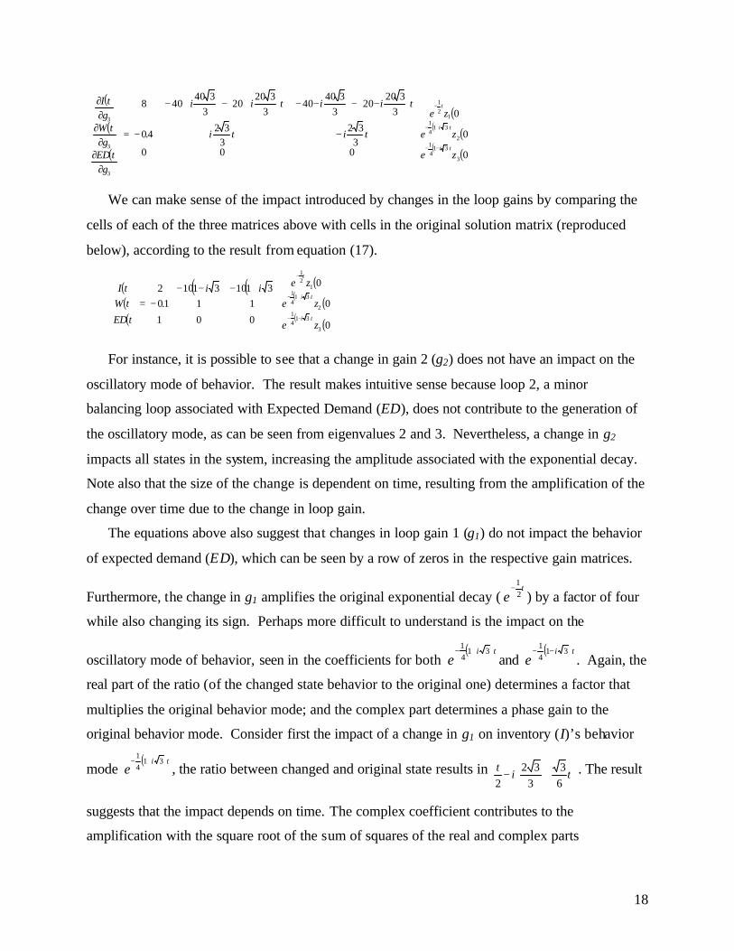
0

0

0

000331

21

331

2140

3320

3320

203

3203

320208

3

3141

2

3141

121

1

1

1

ze

ze

ze

titi.

tiitii

gtED

gtW

gtI

ti

ti

t

;

( )

( )

( )

( )( )

( )( )

( )( ) ( )

−

+

=

∂∂

∂∂∂∂

−−

+−

−

0

0

0

000010

0024

3

314

12

314

11

21

2

2

2

ze

ze

ze

tt.

t

gtED

gtW

gtI

ti

ti

t

;

18

( )

( )

( )

( )( ) ( )( ) ( )

−−

−−

−−

+−

+−

=

∂∂

∂∂∂∂

−−

+−

−

0

0

0

0003

3233240

3320

203

34040

3320

203

340408

3

3141

2

3141

121

3

3

3

ze

ze

ze

titi.

tiitii

gtED

gtW

gtI

ti

ti

t

We can make sense of the impact introduced by changes in the loop gains by comparing the

cells of each of the three matrices above with cells in the original solution matrix (reproduced

below), according to the result from equation (17).

( )( )( )

( ) ( ) ( )( ) ( )( ) ( )

−+−−−

=

−−

+−

−

0

0

0

001

1110311031102

3

3141

2

3141

121

ze

ze

ze

.ii

tED

tWtI

ti

ti

t

For instance, it is possible to see that a change in gain 2 (g2) does not have an impact on the

oscillatory mode of behavior. The result makes intuitive sense because loop 2, a minor

balancing loop associated with Expected Demand (ED), does not contribute to the generation of

the oscillatory mode, as can be seen from eigenvalues 2 and 3. Nevertheless, a change in g2

impacts all states in the system, increasing the amplitude associated with the exponential decay.

Note also that the size of the change is dependent on time, resulting from the amplification of the

change over time due to the change in loop gain.

The equations above also suggest that changes in loop gain 1 (g1) do not impact the behavior

of expected demand (ED), which can be seen by a row of zeros in the respective gain matrices.

Furthermore, the change in g1 amplifies the original exponential decay (t

e 21

−) by a factor of four

while also changing its sign. Perhaps more difficult to understand is the impact on the

oscillatory mode of behavior, seen in the coefficients for both ( )ti

e31

41

+−and

( )tie

3141

−−. Again, the

real part of the ratio (of the changed state behavior to the original one) determines a factor that

multiplies the original behavior mode; and the complex part determines a phase gain to the

original behavior mode. Consider first the impact of a change in g1 on inventory (I)’s behavior

mode ( )ti

e31

41

+−, the ratio between changed and original state results in

+− ti

t63

332

2. The result

suggests that the impact depends on time. The complex coefficient contributes to the

amplification with the square root of the sum of squares of the real and complex parts

19

(22

63

332

2

−−+

t

t ) and to the phase shift by the inverse tangent of the ratio of the real by the

complex parts (

+−−

263

3321 t

ttan ). When time is close to zero ( 0≅t ), the amplification to

the oscillatory mode is given by a factor of 332 and the phase shift is of

2π

− . To compute the

impact on the inventory (I) behavior at a specific time t, it would be required to substitute the

adequate value of time. For instance, at t = 4 the change in g1 causes an amplification to the

oscillatory mode by a factor of 3.05 (since 053328

334

24

22

.==

−+

) and a phase shift of

approximately -49o (since ( ) o1 49332 −≈−−tan ). It is necessary to proceed in a similar way to

compute the impact on different behavior modes. To inform policy it is still required to compute

the overall impact of changes in a loop gain to the overall behavior of a state, by adding the

individual impacts of different modes and selecting the desired behavior modes.

5. Discussion

The motivation for this paper is to provide a mathematical framework to understand the

contribution that changes in link (or loop) gains have on the time path behavior of state variables

in linear dynamic systems. Our research focuses on the analytical computation of the influence

of eigenvalues and eigenvectors on model behavior. This work follows closely the research

tradition established by Forrester (1982). Our work departs from previous efforts in terms of its

focus on analytical results and emphasis on the impact that first time derivatives of eigenvalues

and eigenvectors have on model behavior, instead of eigenvalue elasticities.

The method discussed above has the advantage of introducing an analytical understanding of

the role of eigenvectors to influence behavior in linear systems; it is precise, it is reproducible;

and it provides a standard way to analyze linear dynamic models. Second, the method provides a

direct measure of the impact of different loops on the behavior response of the system. Third,

the method characterizes measures and enumerates how different loops influence different

modes of behavior. Fourth, the method contributes to understanding of transient analysis instead

of simply steady state analysis. Finally, by linearizing a nonlinear system at every point in time,

20

we arrive at a general solution that provides a good approximation of the impact of a change in

link gains to the behavior of state xi.

The method also has a number of shortcomings. First, solutions to the behavior of states in

the system are required to obtain the analytical results. Also, the derivations aimed at the impact

of a change in structure to the behavior of linear systems. While linear systems are used to

derive the main results, consecutive system linearization extends the application to nonlinear

systems. This result is stated but no example is provided. Further research that implements the

computation of eigenvalues, eigenvectors and the first derivatives with respect to the link (and

loop) gains and test different nonlinear models are required to assess the usefulness of the

proposed method. As the linear example suggests, the method poses challenges in terms of

interpreting and evaluating the impact of eigenvector and eigenvalue contribution to behavior

modes.

Despite its current challenges and limitations, we are hopeful that the method provides a

useful step to the analysis of how structure influences behavior as well as a new direction for

future research on the analysis of nonlinear dynamic systems.

6. References Eberlein, R.L. 1989. Simplification and Understanding of Models. System Dynamics Review.

5(1). Forrester, N. 1982. A Dynamic Synthesis of Basic Macroeconomic Policy: Implications for

Stabilization Policy Analysis. Unpublished Ph.D. Thesis, M.I.T., Cambridge, MA. Forrester, N. 1983. Eigenvalue Analysis of Dominant Feedback Analysis. Proceeding of the

1983 International System Dynamics Conference, Plenary Session Papers. System Dynamics Society: Albany, NY. pp178-202.

Gonçalves P, Lertpattarapong C, Hines J. 2000. Implementing formal model analysis.

Proceedings of the 2000 International System Dynamics Conference, Bergen, Norway. System Dynamics Society, Albany, NY.

Güneralp, B. 2005. Towards Coherent Loop Dominance Analysis: Progress in Eigenvalue

Elasticity Analysis. Proceedings of the 2005 International System Dynamics Conference. Boston.

Hines, J. 2005. How to Visit a Great Model Like Yours. Proceedings of the 2005 International

System Dynamics Conference. Boston.

21

Kampmann, C.E. 1996. Feedback Loop Gains and System Behavior. Proceeding of the 1996 International System Dynamics Conference Boston. System Dynamics Society: Albany, NY. pp. 260-263.

Kampmann, C.E. and R. Oliva. 2006. Loop eigenvalue elasticity analysis: Three case studies.

System Dynamics Review (forthcoming). Mojtahedzadeh, M.T. 1996. A Path Taken: Computer-Assisted Heuristics for Understanding

Dynamic Systems. Unpublished Ph.D. Dissertation, Rockefeller College of Public Affairs and Policy, State University of New York at Albany, 1996, Albany NY.

Mojtahedzadeh, M., G. Richardson and D. Andersen. 2004. Using Digest to implement the

pathway participation method for detecting influential system structure. System Dynamics Review. 20(1):1-20.

Oliva, R. 2004. Model structure analysis through graph theory: Partition heuristics and feedback

structure decomposition. System Dynamics Review. 20(4):313-336. Oliva, R. and M. Mojtahedzadeh. 2004. Keep it Simple: Dominance Assessment of Short

Feedback Loops. Proceedings of the 2004 International System Dynamics Conference. Oxford, UK.

Reinschke, KJ. Multivariate Control: A Graph Theoretical Approach. Lecture Notes in Control

and Information Sciences. 1988. Berlin: Springer-Verlag. Richardson GP. 1995. Loop polarity, loop dominance, and the concept of dominant polarity.

System Dynamics Review 11(1): 67-88. Richardson, G.P. Dominant Structure. System Dynamics Review, 1986. 2(1): 68-75. Saleh, M. and P. Davidsen. 2000. An Eigenvalue Approach to Feedback Loop Dominance

Analysis in Non-linear Dynamic Models. Proceedings of the 2000 International System Dynamics Conference. Bergen, Norway.

Saleh, M. and P. Davidsen. 2001. The Origins of Business Cycles. Proceedings of the 2001

International System Dynamics Conference. Atlanta. Saleh, M. 2002. The Characterization of Model Behavior and its Causal Foundation. PhD

Dissertation, University of Bergen, Bergen, Norway. Saleh, M., P. Davidsen and K. Bayoumi. 2005. A Comprehensive Eigenvalue Analysis of

System Dynamics Models. Proceedings of the 2005 International System Dynamics Conference. Boston.

22

Appendix A – The Product of a Complex Number by Complex Exponentials

To understand the implication of multiplying a complex exponential by a complex number,

consider the following example: ( ) ( )ii dceba ++

we can rewrite the exponential as: ( ) ii dcdc eee =+

and by definition ( ) ( )dsindcosed ii +=

so we can rewrite the equation above as: ( ) ( ) ( )( )dsindcosbaec ii ++

( ) ( ) ( )( ) ( ) ( ) ( )( )dsindcosbedsindcosae cc −++ ii

( ) ( )( ) ( ) ( )( )[ ]dsinadcosbdsinbdcosaec ++− i

Multiplying by 1(22

22

ba

ba

+

+ ) and defining ( )φtanab

= , we observe that ( )φcosba

a=

+ 22and

( )φsinba

b=

+ 22 we can rewrite the equation above as:

( ) ( ) ( ) ( ) ( )

++

++

+−

++ dsin

ba

adcosba

bdsinba

bdcosba

aeba c

22222222

22 i

( ) ( ) ( ) ( ) ( )( ) ( ) ( ) ( ) ( )( )[ ]dsincosdcossindsinsindcoscoseba c φφφφ ++−+ i22

Since ( ) ( ) ( ) ( ) ( )( )dsinsindcoscosdcos φφφ −=+ and ( ) ( ) ( ) ( ) ( )( )dsincosdcossindsin φφφ +=+ , we

obtain:

( ) ( ) ( )[ ]φφ ++++ dsindcoseba c i 22

( ) ( )φ+++ dceba i22

( )

++ −

+ ab

tandc

eba1i

22

Therefore, the complex number multiplying the exponential contributes to the amplification

with the square root of the sum of squares of the real and complex parts, and to the phase shift by

the inverse tangent of the ratio of the complex by the real parts. The inverse tangent of (x) is

defined in the interval 22πφπ <<− . The inverse tangent takes a value of zero when x is zero; and

it takes a positive (negative) value when x is positive (negative).

23

Appendix B - How loops influence system behavior?

To understand how changes in loop gains (i.e., the strength of a feedback loop) influence

system behavior, we follow a derivation analogous to the one in section 3. The behavior of each

state in the system xi(t) is described by equation (10), which demonstrates that the behavior of

each state is influenced both by eigenvalues (λi) and eigenvectors (rji).

( ) ( ) ( ) ( )000 221121

nt

nit

it

ii zer...zerzertx nλλλ +++=

While it is more common to write the characteristic polynomial (P(λ)) and eigenvalues in

terms of the link gains (akl), it is also possible to write them in terms of loop gains (gk). Loops,

and their gains, may be a more comprehensive (better) way to describe structure, since modelers

often decide to include (or exclude) loops based on the dynamic hypotheses that they believe are

important in a system. Since we are ultimately interested in how structure drives behavior,

understanding how changes in loop gains influence system behavior may be more appropriate

than looking at how changes in links influence behavior. To capture how loops influence system

behavior, we take the partial derivative of each state in the system xi(t) with respect to its loop

gains. Therefore we take a partial derivative of equation (10), characterizing the behavior of

state xi(t), with respect to a loop gain (gk).

( ) ( ) ( )[ ]00111

nt?

nit?

ikk

i zer...zergg

txn++

∂∂

=∂

∂ (B1)

Which for linear systems, we can write equation as:

( ) ( )∑=

∂∂

+∂∂

=∂

∂ n

jj

t?

k

jji

k

ji

k

i zetg?

rgr

gtx j

1

0 (B2)

Equation (B2) suggests that for each component j (with j =1 to n) characterizing the behavior

of state xi(t), the contribution to the change in behavior of state xi(t) due to the change in loop

gain (gk) is composed of two terms. The first term captures a change in intensity in the mode of

behavior due to the contribution of the partial derivative of the the i-th component of the j-th

eigenvector with respect to loop gain (gk). Analogously, the second term captures a change in

intensity in the mode of behavior due to (a) time, (b) the i-th component of the j-th eigenvector

and (c) the partial derivative of the i-th eigenvalue (λi) with respect to loop gain (gk).

24

With his suggestion of finding the characteristic polynomial in terms of the loop gains,

Forrester (1983) extended the results of link sensitivity and link elasticity to loop sensitivity and

loop elasticity.

k

ik g

Si ∂

∂λλ = and

i

k

k

iik

gg

Eλ∂

∂λ= (B3)

In addition, we can extend the concept of link eigenvector sensitivity and elasticity

introduced in the previous section to loop eigenvector sensitivity and eigenvector elasticity with

respect to loop gain or loop gain eigenvector elasticity.

k

ijkr g

rS

ij ∂∂

= and j

jr r

rj

k

kk

gg

E

∂∂

= (B4)

Equation (B2) provides an integrated way to assess how loop eigenvalue and eigenvector

sensitivity (i.e., the partial derivatives with respect to a loop gain) work together to influence

system behavior. In particular, we can rewrite equation (B2) as:

( ) ( ) ( )∑=

+=∂

∂ n

jj

t?kjikr

k

i zetSrSg

tx j

jij1

0λ (B5)

• Loop eigenvector sensitivity k

ijkr g

rS

ij ∂∂

= captures a change in intensity in the mode

of behavior ( ( )0jt? ze j ) due to a change in a loop gain (gk);

• Loop eigenvalue sensitivity k

ik g

Si ∂

∂λλ = captures the change in the behavior mode

(i.e., λi) due to a change in the loop gain (gk); and

• The contribution of the eigenvalue elasticity changes with time, becoming the

main determinant of behavior over time.

Loop gain eigenvalue elasticity captures changes in the mode of behavior, that is, it measures

whether the state will have faster or slower growth, decay, or oscillations. In turn, loop gain

eigenvector elasticity capture changes in the intensity of that behavior mode, that is, it measures

the importance of that behavior mode to the overall behavior of the state. To compute the

eigenvalues in terms of loop gains readers are directed to Forrester (1983), Kampmann (1996),

Gonçalves, Hines and Lertpattarapong (2000) and Kampmann and Oliva (2006).