eigenmath manual - github pages
TRANSCRIPT
Eigenmath Manual
October 17, 2021
Contents
1 Introduction 21.1 Syntax . . . . . . . . . . . . . . . . . . . . . . . . . . . . . . . . . . . . . . . . . . . 21.2 Testing for equality . . . . . . . . . . . . . . . . . . . . . . . . . . . . . . . . . . . . 31.3 Arithmetic . . . . . . . . . . . . . . . . . . . . . . . . . . . . . . . . . . . . . . . . . 41.4 Exponents . . . . . . . . . . . . . . . . . . . . . . . . . . . . . . . . . . . . . . . . . 41.5 Symbols . . . . . . . . . . . . . . . . . . . . . . . . . . . . . . . . . . . . . . . . . . 51.6 User defined functions . . . . . . . . . . . . . . . . . . . . . . . . . . . . . . . . . . 61.7 Complex numbers . . . . . . . . . . . . . . . . . . . . . . . . . . . . . . . . . . . . . 71.8 Linear algebra . . . . . . . . . . . . . . . . . . . . . . . . . . . . . . . . . . . . . . . 81.9 Component arithmetic . . . . . . . . . . . . . . . . . . . . . . . . . . . . . . . . . . 10
2 Calculus 112.1 Derivative . . . . . . . . . . . . . . . . . . . . . . . . . . . . . . . . . . . . . . . . . 112.2 Gradient . . . . . . . . . . . . . . . . . . . . . . . . . . . . . . . . . . . . . . . . . . 112.3 Template functions . . . . . . . . . . . . . . . . . . . . . . . . . . . . . . . . . . . . 112.4 Integral . . . . . . . . . . . . . . . . . . . . . . . . . . . . . . . . . . . . . . . . . . 122.5 Arc length . . . . . . . . . . . . . . . . . . . . . . . . . . . . . . . . . . . . . . . . . 132.6 Line integrals . . . . . . . . . . . . . . . . . . . . . . . . . . . . . . . . . . . . . . . 152.7 Surface area . . . . . . . . . . . . . . . . . . . . . . . . . . . . . . . . . . . . . . . . 162.8 Surface integrals . . . . . . . . . . . . . . . . . . . . . . . . . . . . . . . . . . . . . . 182.9 Green’s theorem . . . . . . . . . . . . . . . . . . . . . . . . . . . . . . . . . . . . . . 192.10 Stokes’ theorem . . . . . . . . . . . . . . . . . . . . . . . . . . . . . . . . . . . . . . 20
3 Quantum Computing 22
4 Function Reference 25
5 Tricks 42
1
1 Introduction
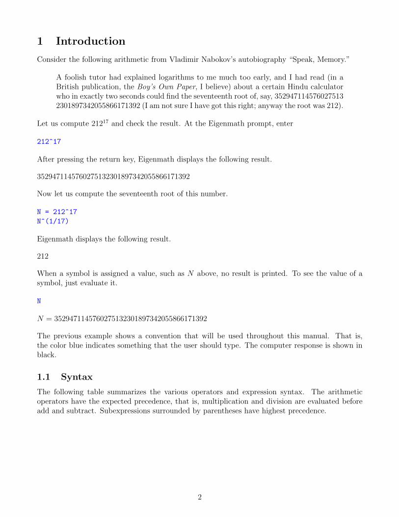
Consider the following arithmetic from Vladimir Nabokov’s autobiography “Speak, Memory.”
A foolish tutor had explained logarithms to me much too early, and I had read (in aBritish publication, the Boy’s Own Paper, I believe) about a certain Hindu calculatorwho in exactly two seconds could find the seventeenth root of, say, 3529471145760275132301897342055866171392 (I am not sure I have got this right; anyway the root was 212).
Let us compute 21217 and check the result. At the Eigenmath prompt, enter
212^17
After pressing the return key, Eigenmath displays the following result.
3529471145760275132301897342055866171392
Now let us compute the seventeenth root of this number.
N = 212^17
N^(1/17)
Eigenmath displays the following result.
212
When a symbol is assigned a value, such as N above, no result is printed. To see the value of asymbol, just evaluate it.
N
N = 3529471145760275132301897342055866171392
The previous example shows a convention that will be used throughout this manual. That is,the color blue indicates something that the user should type. The computer response is shown inblack.
1.1 Syntax
The following table summarizes the various operators and expression syntax. The arithmeticoperators have the expected precedence, that is, multiplication and division are evaluated beforeadd and subtract. Subexpressions surrounded by parentheses have highest precedence.
2
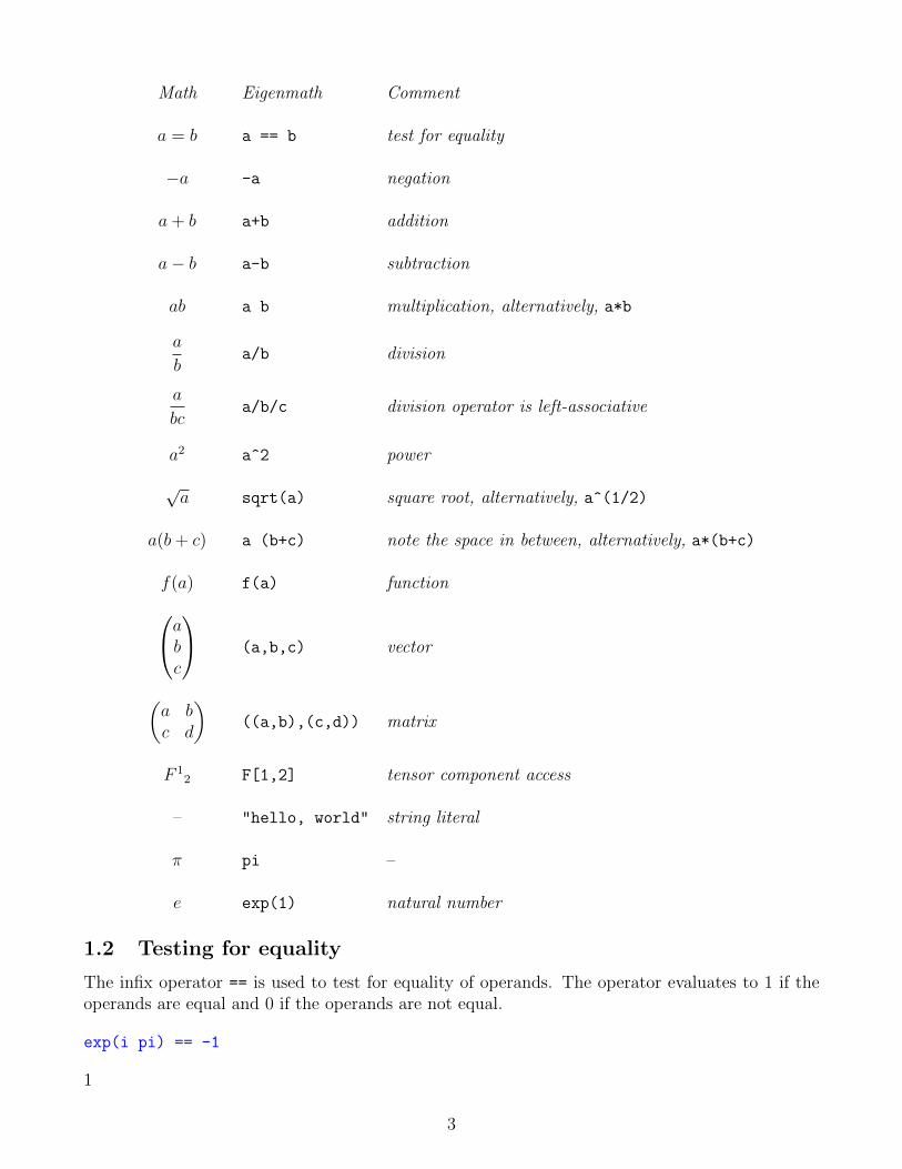
Math Eigenmath Comment
a = b a == b test for equality
−a -a negation
a+ b a+b addition
a− b a-b subtraction
ab a b multiplication, alternatively, a*b
a
ba/b division
a
bca/b/c division operator is left-associative
a2 a^2 power
√a sqrt(a) square root, alternatively, a^(1/2)
a(b+ c) a (b+c) note the space in between, alternatively, a*(b+c)
f(a) f(a) functionabc
(a,b,c) vector
(a bc d
)((a,b),(c,d)) matrix
F 12 F[1,2] tensor component access
– "hello, world" string literal
π pi –
e exp(1) natural number
1.2 Testing for equality
The infix operator == is used to test for equality of operands. The operator evaluates to 1 if theoperands are equal and 0 if the operands are not equal.
exp(i pi) == -1
1
3
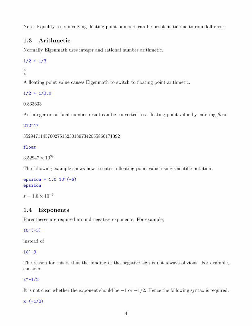
Note: Equality tests involving floating point numbers can be problematic due to roundoff error.
1.3 Arithmetic
Normally Eigenmath uses integer and rational number arithmetic.
1/2 + 1/3
56
A floating point value causes Eigenmath to switch to floating point arithmetic.
1/2 + 1/3.0
0.833333
An integer or rational number result can be converted to a floating point value by entering float.
212^17
3529471145760275132301897342055866171392
float
3.52947× 1039
The following example shows how to enter a floating point value using scientific notation.
epsilon = 1.0 10^(-6)
epsilon
ε = 1.0× 10⁻⁶
1.4 Exponents
Parentheses are required around negative exponents. For example,
10^(-3)
instead of
10^-3
The reason for this is that the binding of the negative sign is not always obvious. For example,consider
x^-1/2
It is not clear whether the exponent should be −1 or −1/2. Hence the following syntax is required.
x^(-1/2)
4
In general, parentheses are always required when the exponent is an expression. For example,x^1/2 is evaluated as (x1)/2 which is probably not the desired result.
x^1/2
12x
Using x^(1/2) yields the desired result.
x^(1/2)
x1/2
1.5 Symbols
As we saw earlier, symbols are defined using an equals sign.
N = 212^17
No result is printed when a symbol is defined. To see the value of a symbol, just evaluate it.
N
N = 3529471145760275132301897342055866171392
Symbols can have more that one letter. Everything after the first letter is displayed as a subscript.
NA = 6.02214 10^23
NA
NA = 6.02214× 10²³
A symbol can be the name of a Greek letter.
xi = 1/2
xi
ξ = 12
Greek letters can appear in subscripts.
Amu = 2.0
Amu
Aµ = 2.0
The following example shows how Eigenmath scans the entire symbol to find Greek letters.
alphamunu = 1
alphamunu
5
αµν = 1
When a symbolic chain is defined, Eigenmath follows the chain as far as possible. The followingexample sets A = B followed by B = C. Then when A is evaluated, the result is C.
A = B
B = C
A
A = C
Although A = C is printed, inside the program the binding of A is still B, as can be seen with thebinding function.
binding(A)
B
The quote function returns its argument unevaluated and can be used to clear a symbol. Thefollowing example clears A so that its evaluation goes back to being A instead of C.
A = quote(A)
A
A
1.6 User defined functions
Most of the functions commonly used in math and physics are included in Eigenmath. See theReference section at the end of the manual for a complete list. There is also a facility for the userto define additional functions.
User functions are defined using the syntax function-name ( arg-list ) = expr where arg-list is acomma separated list of zero to nine symbols that receive arguments. Unlike symbol definitions,expr is not evaluated when function-name is defined. Instead, expr is evaluated when function-name is used in a subsequent computation.
The following example defines a sinc function and evaluates it at π/2.
f(x) = sin(x)/x
f(pi/2)
2
π
After a user function is defined, expr can be recalled using the binding function.
binding(f)
6
sin(x)
x
If local symbols are needed in a function, they can be appended to arg-list. (The caller does nothave to supply all the arguments.) The following example uses Rodrigues’s formula to computean associated Legendre function of cos θ.
Pmn (x) =
1
2n n!(1− x2)m/2 d
n+m
dxn+m(x2 − 1)n
Function P below first computes Pmn (x) for local variable x and then uses eval to replace x with
f . In this case, f = cos θ.
x = 123 -- global x in use, need local x in P
P(f,n,m,x) = eval(1/(2^n n!) (1 - x^2)^(m/2) d((x^2 - 1)^n,x,n + m),x,f)
P(cos(theta),2,0) -- arguments f, n, m, but not x
32
cos(θ)2 − 12
The scope of function arguments is limited to the function definition.
1.7 Complex numbers
When Eigenmath starts up, it defines symbol i as i =√−1. Symbol i can be redefined and used
for some other purpose if need be.
Complex quantities can be entered in either rectangular or polar form.
a + i b
a+ ib
exp(1/3 i pi)
exp(13iπ)
Converting a complex number to rectangular or polar coordinates causes simplification of mixedforms.
A = 1 + i
B = sqrt(2) exp(1/4 i pi)
A - B
1 + i− 21/2 exp(14iπ)
rect(last)
0
Rectangular complex quantities, when raised to a power, are multiplied out.
7
(a + i b)^2
a2 − b2 + 2iab
When a and b are numerical and the power is negative, the evaluation is done as follows.
(a+ ib)−n =
(a− ib
(a+ ib)(a− ib)
)n=
(a− iba2 + b2
)nHere are a few examples.
1/(2 - i)
25
+ 15i
(-1 + 3 i)/(2 - i)
−1 + i
The absolute value of a complex number returns its magnitude.
abs(3 + 4 i)
5
The imaginary unit can be changed from i to j by defining j =√−1.
j = sqrt(-1)
sqrt(-4)
2j
1.8 Linear algebra
The dot function is used to multiply tensors. For example, let
A =
(1 23 4
)and x =
(x1x2
)The product Ax is computed as follows.
A = ((1,2),(3,4))
x = (x1,x2)
dot(A,x)[x1 + 2x23x1 + 4x2
]The following example shows how to use dot and inv to solve for the vector X in AX = B.
8
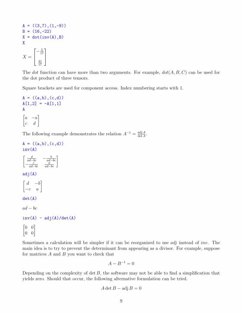
A = ((3,7),(1,-9))
B = (16,-22)
X = dot(inv(A),B)
X
X =
− 517
4117
The dot function can have more than two arguments. For example, dot(A,B,C) can be used forthe dot product of three tensors.
Square brackets are used for component access. Index numbering starts with 1.
A = ((a,b),(c,d))
A[1,2] = -A[1,1]
A[a −ac d
]The following example demonstrates the relation A−1 = adjA
detA.
A = ((a,b),(c,d))
inv(A)[d
ad−bc − bad−bc
− cad−bc
aad−bc
]adj(A)[d −b−c a
]det(A)
ad− bc
inv(A) - adj(A)/det(A)[0 00 0
]Sometimes a calculation will be simpler if it can be reorganized to use adj instead of inv. Themain idea is to try to prevent the determinant from appearing as a divisor. For example, supposefor matrices A and B you want to check that
A−B−1 = 0
Depending on the complexity of detB, the software may not be able to find a simplification thatyields zero. Should that occur, the following alternative formulation can be tried.
A detB − adjB = 0
9
1.9 Component arithmetic
Tensor plus scalar adds the scalar to each component of the tensor.
(x,y,z) + 10x+ 10y + 10z + 10
The product of two tensors is the Hadamard product.
A = ((1,2),(3,4))
B = ((a,b),(c,d))
A B[a 2b3c 4d
]Tensor raised to a power raises each component to the power.
(x,y,z)^2x2y2z2
10
2 Calculus
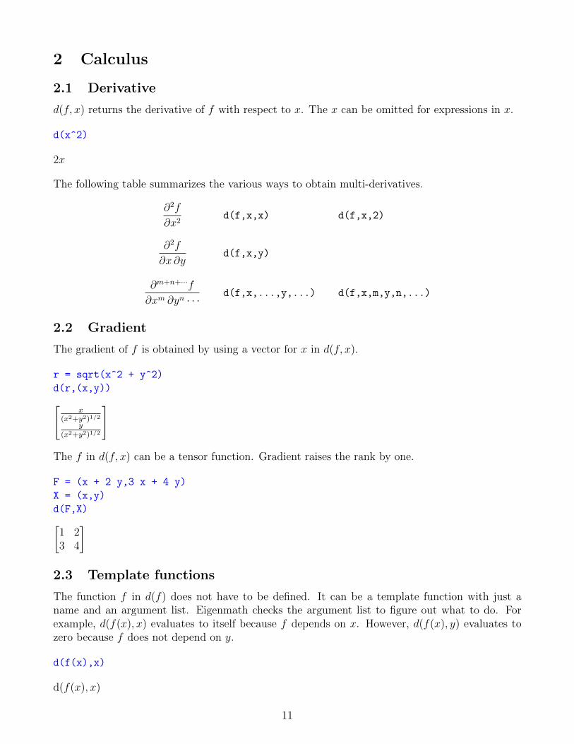
2.1 Derivative
d(f, x) returns the derivative of f with respect to x. The x can be omitted for expressions in x.
d(x^2)
2x
The following table summarizes the various ways to obtain multi-derivatives.
∂2f
∂x2d(f,x,x) d(f,x,2)
∂2f
∂x ∂yd(f,x,y)
∂m+n+···f
∂xm ∂yn · · ·d(f,x,...,y,...) d(f,x,m,y,n,...)
2.2 Gradient
The gradient of f is obtained by using a vector for x in d(f, x).
r = sqrt(x^2 + y^2)
d(r,(x,y))[x
(x2+y2)1/2y
(x2+y2)1/2
]
The f in d(f, x) can be a tensor function. Gradient raises the rank by one.
F = (x + 2 y,3 x + 4 y)
X = (x,y)
d(F,X)[1 23 4
]
2.3 Template functions
The function f in d(f) does not have to be defined. It can be a template function with just aname and an argument list. Eigenmath checks the argument list to figure out what to do. Forexample, d(f(x), x) evaluates to itself because f depends on x. However, d(f(x), y) evaluates tozero because f does not depend on y.
d(f(x),x)
d(f(x), x)
11
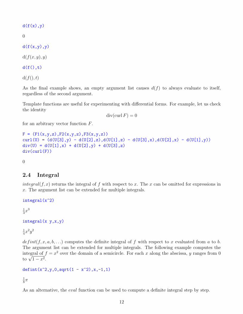
d(f(x),y)
0
d(f(x,y),y)
d(f(x, y), y)
d(f(),t)
d(f(), t)
As the final example shows, an empty argument list causes d(f) to always evaluate to itself,regardless of the second argument.
Template functions are useful for experimenting with differential forms. For example, let us checkthe identity
div(curlF ) = 0
for an arbitrary vector function F .
F = (F1(x,y,z),F2(x,y,z),F3(x,y,z))
curl(U) = (d(U[3],y) - d(U[2],z),d(U[1],z) - d(U[3],x),d(U[2],x) - d(U[1],y))
div(U) = d(U[1],x) + d(U[2],y) + d(U[3],z)
div(curl(F))
0
2.4 Integral
integral(f, x) returns the integral of f with respect to x. The x can be omitted for expressions inx. The argument list can be extended for multiple integrals.
integral(x^2)
13x3
integral(x y,x,y)
14x2y2
defint(f, x, a, b, . . .) computes the definite integral of f with respect to x evaluated from a to b.The argument list can be extended for multiple integrals. The following example computes theintegral of f = x2 over the domain of a semicircle. For each x along the abscissa, y ranges from 0to√
1− x2.
defint(x^2,y,0,sqrt(1 - x^2),x,-1,1)
18π
As an alternative, the eval function can be used to compute a definite integral step by step.
12
I = integral(x^2,y)
I = eval(I,y,sqrt(1 - x^2)) - eval(I,y,0)
I = integral(I,x)
eval(I,x,1) - eval(I,x,-1)
18π
Here is a useful trick. Difficult integrals involving sine and cosine can often be solved by usingexponentials. Trigonometric simplifications involving powers and multiple angles turn into simplealgebra in the exponential domain. For example, the definite integral∫ 2π
0
(sin4 t− 2 cos3(t/2) sin t
)dt
can be solved as follows.
f = sin(t)^4 - 2 cos(t/2)^3 sin(t)
f = circexp(f)
defint(f,t,0,2pi)
−165
+ 34π
Here is a check of the result.
g = integral(f,t)
f - d(g,t)
0
2.5 Arc length
Let g(t) be a function that draws a curve. The arc length from g(a) to g(b) is given by∫ b
a
|g′(t)| dt
where |g′(t)| is the length of the tangent vector at g(t). The integral sums over all of the tangentlengths to arrive at the total length from a to b. For example, let us measure the length of x2 fromx = 0 to x = 1. A suitable g(t) for the arc x2 is
g(t) = (t, t2), 0 ≤ t ≤ 1
Hence one Eigenmath solution for computing the arc length is
x = t
y = t^2
g = (x,y)
defint(abs(d(g,t)),t,0,1)
12
51/2 + 14
log(51/2 + 2)
13
float
1.47894
As expected, the result is greater than√
2 ≈ 1.414, the length of the diagonal from (0, 0) to (1, 1).
The result seems rather complicated given that we started with a simple parabola. Let us inspect|g′(t)| to see why.
g
g =
[tt2
]d(g,t)[
12t
]abs(d(g,t))
(4t2 + 1)1/2
The following script does a discrete computation of the arc length by dividing the curve into 100pieces.
g(t) = (t,t^2)
h(k) = abs(g(k/100.0) - g((k-1)/100.0))
sum(k,1,100,h(k))
1.47894
As expected, the discrete result matches the analytic result.
Find the length of the curve y = x3/2 from the origin to x = 43.
x = t
y = x^(3/2)
g = (x,y)
defint(abs(d(g,x)),x,0,4/3)
5627
Because of the way t is substituted for x, the following code yields the same result.
g = (t,t^(3/2))
defint(abs(d(g,t)),t,0,4/3)
5627
14
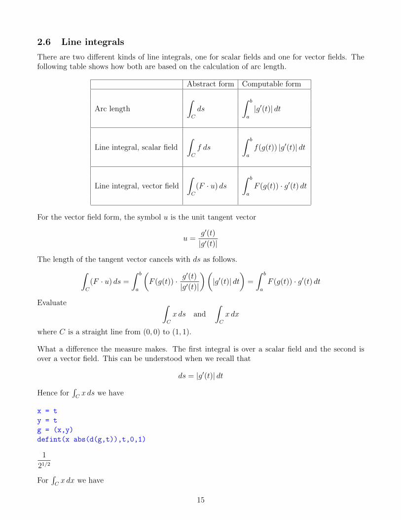
2.6 Line integrals
There are two different kinds of line integrals, one for scalar fields and one for vector fields. Thefollowing table shows how both are based on the calculation of arc length.
Abstract form Computable form
Arc length
∫C
ds
∫ b
a
|g′(t)| dt
Line integral, scalar field
∫C
f ds
∫ b
a
f(g(t)) |g′(t)| dt
Line integral, vector field
∫C
(F · u) ds
∫ b
a
F (g(t)) · g′(t) dt
For the vector field form, the symbol u is the unit tangent vector
u =g′(t)
|g′(t)|
The length of the tangent vector cancels with ds as follows.∫C
(F · u) ds =
∫ b
a
(F (g(t)) · g
′(t)
|g′(t)|
)(|g′(t)| dt
)=
∫ b
a
F (g(t)) · g′(t) dt
Evaluate ∫C
x ds and
∫C
x dx
where C is a straight line from (0, 0) to (1, 1).
What a difference the measure makes. The first integral is over a scalar field and the second isover a vector field. This can be understood when we recall that
ds = |g′(t)| dt
Hence for∫Cx ds we have
x = t
y = t
g = (x,y)
defint(x abs(d(g,t)),t,0,1)
1
21/2
For∫Cx dx we have
15
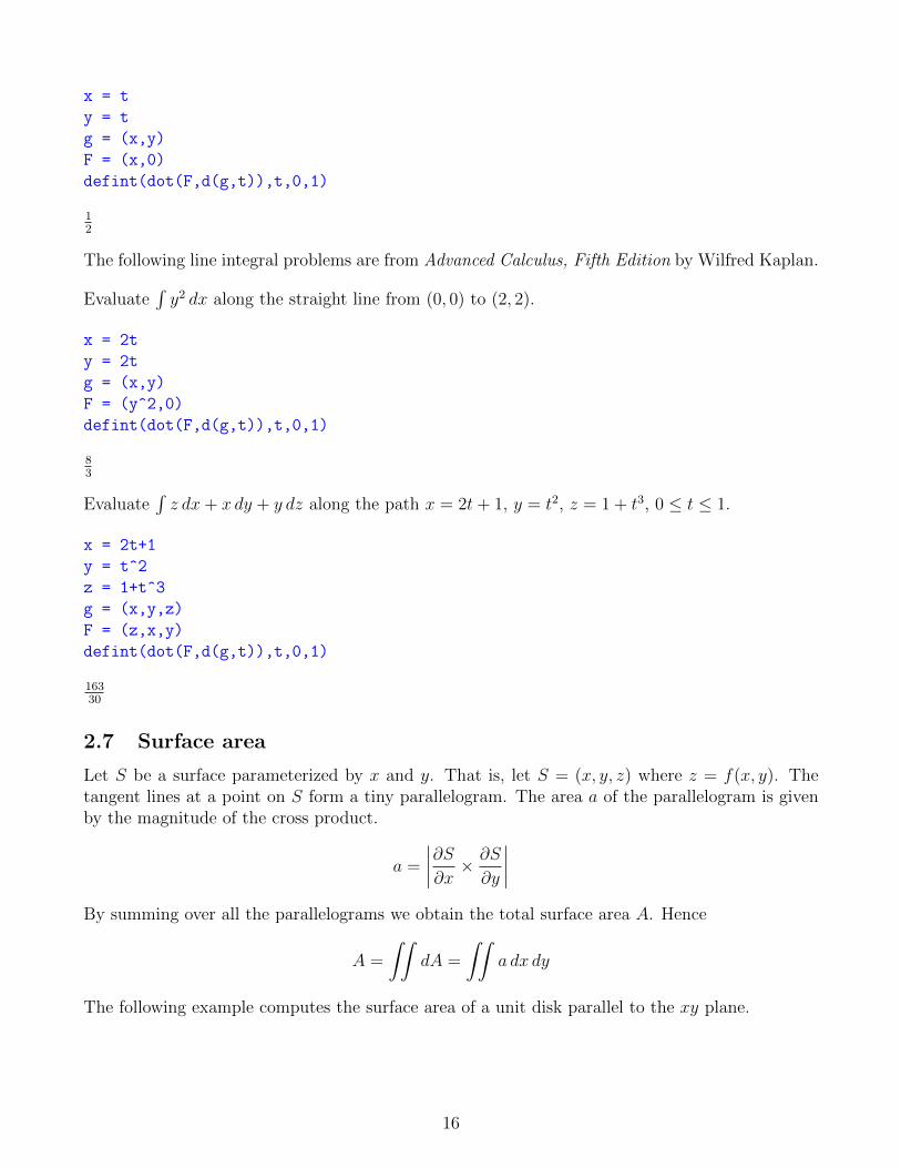
x = t
y = t
g = (x,y)
F = (x,0)
defint(dot(F,d(g,t)),t,0,1)
12
The following line integral problems are from Advanced Calculus, Fifth Edition by Wilfred Kaplan.
Evaluate∫y2 dx along the straight line from (0, 0) to (2, 2).
x = 2t
y = 2t
g = (x,y)
F = (y^2,0)
defint(dot(F,d(g,t)),t,0,1)
83
Evaluate∫z dx+ x dy + y dz along the path x = 2t+ 1, y = t2, z = 1 + t3, 0 ≤ t ≤ 1.
x = 2t+1
y = t^2
z = 1+t^3
g = (x,y,z)
F = (z,x,y)
defint(dot(F,d(g,t)),t,0,1)
16330
2.7 Surface area
Let S be a surface parameterized by x and y. That is, let S = (x, y, z) where z = f(x, y). Thetangent lines at a point on S form a tiny parallelogram. The area a of the parallelogram is givenby the magnitude of the cross product.
a =
∣∣∣∣∂S∂x × ∂S
∂y
∣∣∣∣By summing over all the parallelograms we obtain the total surface area A. Hence
A =
∫∫dA =
∫∫a dx dy
The following example computes the surface area of a unit disk parallel to the xy plane.
16
M1 = ((0,0,0),(0,0,-1),(0,1,0))
M2 = ((0,0,1),(0,0,0),(-1,0,0))
M3 = ((0,-1,0),(1,0,0),(0,0,0))
M = (M1,M2,M3)
cross(u,v) = dot(u,M,v)
z = 2
S = (x,y,z)
a = abs(cross(d(S,x),d(S,y)))
defint(a,y,-sqrt(1 - x^2),sqrt(1 - x^2),x,-1,1)
π
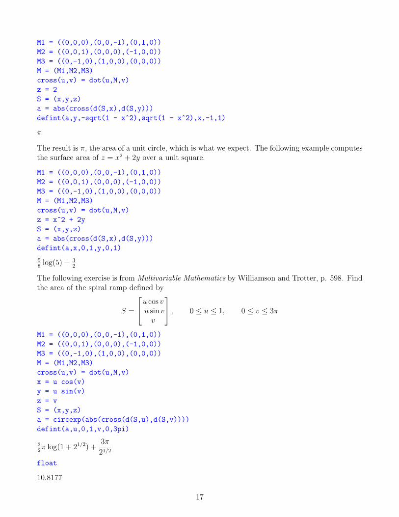
The result is π, the area of a unit circle, which is what we expect. The following example computesthe surface area of z = x2 + 2y over a unit square.
M1 = ((0,0,0),(0,0,-1),(0,1,0))
M2 = ((0,0,1),(0,0,0),(-1,0,0))
M3 = ((0,-1,0),(1,0,0),(0,0,0))
M = (M1,M2,M3)
cross(u,v) = dot(u,M,v)
z = x^2 + 2y
S = (x,y,z)
a = abs(cross(d(S,x),d(S,y)))
defint(a,x,0,1,y,0,1)
58
log(5) + 32
The following exercise is from Multivariable Mathematics by Williamson and Trotter, p. 598. Findthe area of the spiral ramp defined by
S =
u cos vu sin vv
, 0 ≤ u ≤ 1, 0 ≤ v ≤ 3π
M1 = ((0,0,0),(0,0,-1),(0,1,0))
M2 = ((0,0,1),(0,0,0),(-1,0,0))
M3 = ((0,-1,0),(1,0,0),(0,0,0))
M = (M1,M2,M3)
cross(u,v) = dot(u,M,v)
x = u cos(v)
y = u sin(v)
z = v
S = (x,y,z)
a = circexp(abs(cross(d(S,u),d(S,v))))
defint(a,u,0,1,v,0,3pi)
32π log(1 + 21/2) +
3π
21/2
float
10.8177
17
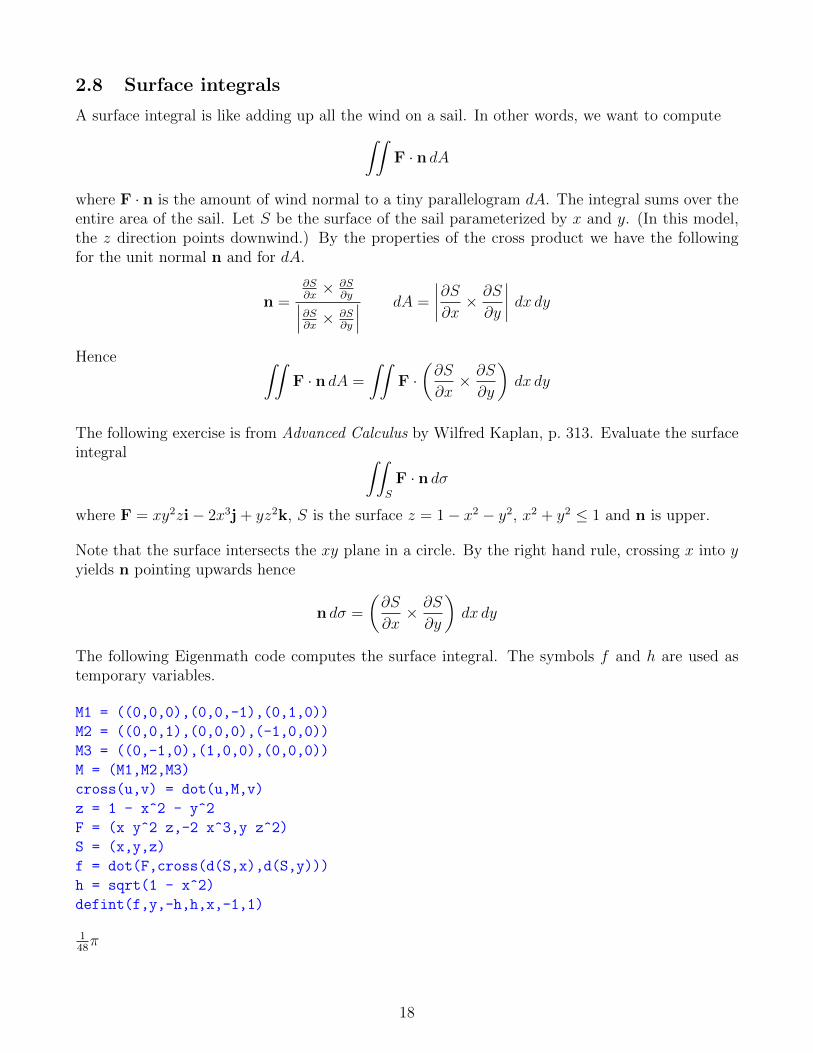
2.8 Surface integrals
A surface integral is like adding up all the wind on a sail. In other words, we want to compute∫∫F · n dA
where F · n is the amount of wind normal to a tiny parallelogram dA. The integral sums over theentire area of the sail. Let S be the surface of the sail parameterized by x and y. (In this model,the z direction points downwind.) By the properties of the cross product we have the followingfor the unit normal n and for dA.
n =
∂S∂x× ∂S
∂y∣∣∣∂S∂x × ∂S∂y
∣∣∣ dA =
∣∣∣∣∂S∂x × ∂S
∂y
∣∣∣∣ dx dyHence ∫∫
F · n dA =
∫∫F ·(∂S
∂x× ∂S
∂y
)dx dy
The following exercise is from Advanced Calculus by Wilfred Kaplan, p. 313. Evaluate the surfaceintegral ∫∫
S
F · n dσ
where F = xy2zi− 2x3j + yz2k, S is the surface z = 1− x2 − y2, x2 + y2 ≤ 1 and n is upper.
Note that the surface intersects the xy plane in a circle. By the right hand rule, crossing x into yyields n pointing upwards hence
n dσ =
(∂S
∂x× ∂S
∂y
)dx dy
The following Eigenmath code computes the surface integral. The symbols f and h are used astemporary variables.
M1 = ((0,0,0),(0,0,-1),(0,1,0))
M2 = ((0,0,1),(0,0,0),(-1,0,0))
M3 = ((0,-1,0),(1,0,0),(0,0,0))
M = (M1,M2,M3)
cross(u,v) = dot(u,M,v)
z = 1 - x^2 - y^2
F = (x y^2 z,-2 x^3,y z^2)
S = (x,y,z)
f = dot(F,cross(d(S,x),d(S,y)))
h = sqrt(1 - x^2)
defint(f,y,-h,h,x,-1,1)
148π
18
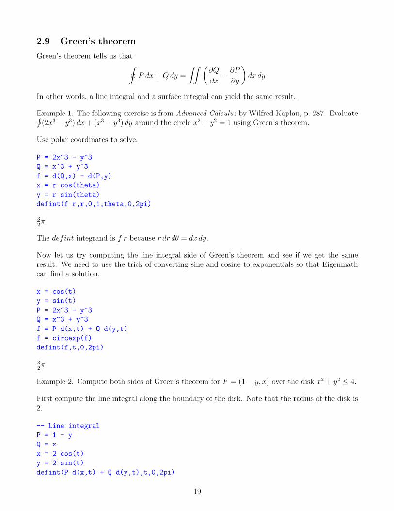
2.9 Green’s theorem
Green’s theorem tells us that∮P dx+Qdy =
∫∫ (∂Q
∂x− ∂P
∂y
)dx dy
In other words, a line integral and a surface integral can yield the same result.
Example 1. The following exercise is from Advanced Calculus by Wilfred Kaplan, p. 287. Evaluate∮(2x3 − y3) dx+ (x3 + y3) dy around the circle x2 + y2 = 1 using Green’s theorem.
Use polar coordinates to solve.
P = 2x^3 - y^3
Q = x^3 + y^3
f = d(Q,x) - d(P,y)
x = r cos(theta)
y = r sin(theta)
defint(f r,r,0,1,theta,0,2pi)
32π
The defint integrand is f r because r dr dθ = dx dy.
Now let us try computing the line integral side of Green’s theorem and see if we get the sameresult. We need to use the trick of converting sine and cosine to exponentials so that Eigenmathcan find a solution.
x = cos(t)
y = sin(t)
P = 2x^3 - y^3
Q = x^3 + y^3
f = P d(x,t) + Q d(y,t)
f = circexp(f)
defint(f,t,0,2pi)
32π
Example 2. Compute both sides of Green’s theorem for F = (1− y, x) over the disk x2 + y2 ≤ 4.
First compute the line integral along the boundary of the disk. Note that the radius of the disk is2.
-- Line integral
P = 1 - y
Q = x
x = 2 cos(t)
y = 2 sin(t)
defint(P d(x,t) + Q d(y,t),t,0,2pi)
19
8π
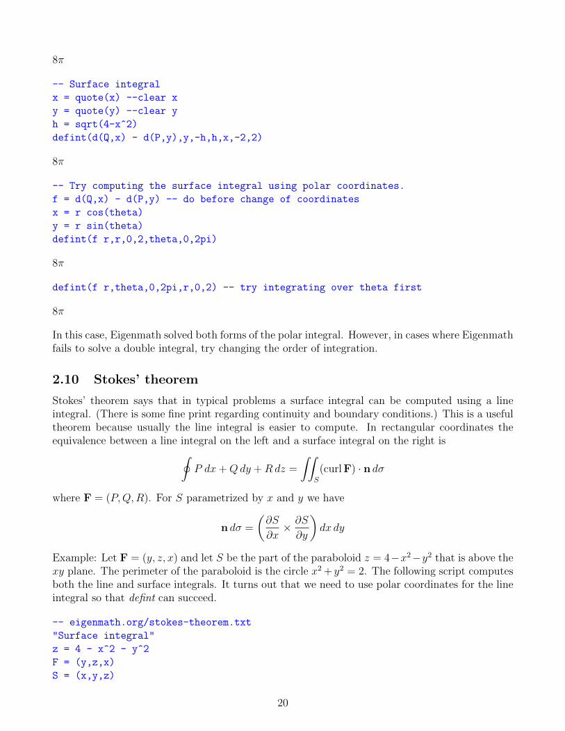
-- Surface integral
x = quote(x) --clear x
y = quote(y) --clear y
h = sqrt(4-x^2)
defint(d(Q,x) - d(P,y),y,-h,h,x,-2,2)
8π
-- Try computing the surface integral using polar coordinates.
f = d(Q,x) - d(P,y) -- do before change of coordinates
x = r cos(theta)
y = r sin(theta)
defint(f r,r,0,2,theta,0,2pi)
8π
defint(f r,theta,0,2pi,r,0,2) -- try integrating over theta first
8π
In this case, Eigenmath solved both forms of the polar integral. However, in cases where Eigenmathfails to solve a double integral, try changing the order of integration.
2.10 Stokes’ theorem
Stokes’ theorem says that in typical problems a surface integral can be computed using a lineintegral. (There is some fine print regarding continuity and boundary conditions.) This is a usefultheorem because usually the line integral is easier to compute. In rectangular coordinates theequivalence between a line integral on the left and a surface integral on the right is∮
P dx+Qdy +Rdz =
∫∫S
(curl F) · n dσ
where F = (P,Q,R). For S parametrized by x and y we have
n dσ =
(∂S
∂x× ∂S
∂y
)dx dy
Example: Let F = (y, z, x) and let S be the part of the paraboloid z = 4−x2−y2 that is above thexy plane. The perimeter of the paraboloid is the circle x2 + y2 = 2. The following script computesboth the line and surface integrals. It turns out that we need to use polar coordinates for the lineintegral so that defint can succeed.
-- eigenmath.org/stokes-theorem.txt
"Surface integral"
z = 4 - x^2 - y^2
F = (y,z,x)
S = (x,y,z)
20
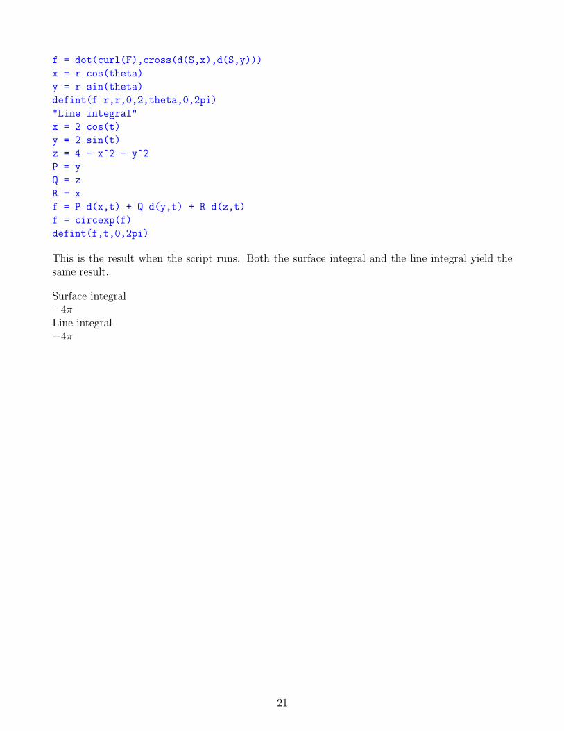
f = dot(curl(F),cross(d(S,x),d(S,y)))
x = r cos(theta)
y = r sin(theta)
defint(f r,r,0,2,theta,0,2pi)
"Line integral"
x = 2 cos(t)
y = 2 sin(t)
z = 4 - x^2 - y^2
P = y
Q = z
R = x
f = P d(x,t) + Q d(y,t) + R d(z,t)
f = circexp(f)
defint(f,t,0,2pi)
This is the result when the script runs. Both the surface integral and the line integral yield thesame result.
Surface integral−4πLine integral−4π
21
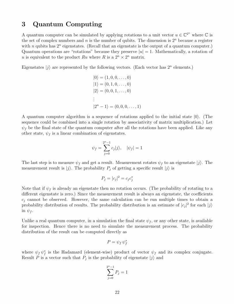
3 Quantum Computing
A quantum computer can be simulated by applying rotations to a unit vector u ∈ C2n where C isthe set of complex numbers and n is the number of qubits. The dimension is 2n because a registerwith n qubits has 2n eigenstates. (Recall that an eigenstate is the output of a quantum computer.)Quantum operations are “rotations” because they preserve |u| = 1. Mathematically, a rotation ofu is equivalent to the product Ru where R is a 2n × 2n matrix.
Eigenstates |j〉 are represented by the following vectors. (Each vector has 2n elements.)
|0〉 = (1, 0, 0, . . . , 0)
|1〉 = (0, 1, 0, . . . , 0)
|2〉 = (0, 0, 1, . . . , 0)
...
|2n − 1〉 = (0, 0, 0, . . . , 1)
A quantum computer algorithm is a sequence of rotations applied to the initial state |0〉. (Thesequence could be combined into a single rotation by associativity of matrix multiplication.) Letψf be the final state of the quantum computer after all the rotations have been applied. Like anyother state, ψf is a linear combination of eigenstates.
ψf =2n−1∑j=0
cj|j〉, |ψf | = 1
The last step is to measure ψf and get a result. Measurement rotates ψf to an eigenstate |j〉. Themeasurement result is |j〉. The probability Pj of getting a specific result |j〉 is
Pj = |cj|2 = cjc∗j
Note that if ψf is already an eigenstate then no rotation occurs. (The probability of rotating to adifferent eigenstate is zero.) Since the measurement result is always an eigenstate, the coefficientscj cannot be observed. However, the same calculation can be run multiple times to obtain aprobability distribution of results. The probability distribution is an estimate of |cj|2 for each |j〉in ψf .
Unlike a real quantum computer, in a simulation the final state ψf , or any other state, is availablefor inspection. Hence there is no need to simulate the measurement process. The probabilitydistribution of the result can be computed directly as
P = ψf ψ∗f
where ψf ψ∗f is the Hadamard (element-wise) product of vector ψf and its complex conjugate.
Result P is a vector such that Pj is the probability of eigenstate |j〉 and
2n−1∑j=0
Pj = 1
22
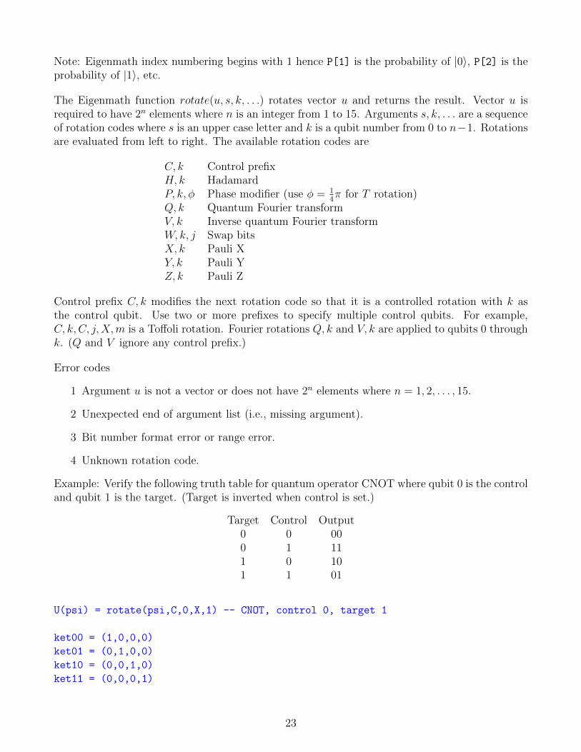
Note: Eigenmath index numbering begins with 1 hence P[1] is the probability of |0〉, P[2] is theprobability of |1〉, etc.
The Eigenmath function rotate(u, s, k, . . .) rotates vector u and returns the result. Vector u isrequired to have 2n elements where n is an integer from 1 to 15. Arguments s, k, . . . are a sequenceof rotation codes where s is an upper case letter and k is a qubit number from 0 to n−1. Rotationsare evaluated from left to right. The available rotation codes are
C, k Control prefixH, k HadamardP, k, φ Phase modifier (use φ = 1
4π for T rotation)
Q, k Quantum Fourier transformV, k Inverse quantum Fourier transformW,k, j Swap bitsX, k Pauli XY, k Pauli YZ, k Pauli Z
Control prefix C, k modifies the next rotation code so that it is a controlled rotation with k asthe control qubit. Use two or more prefixes to specify multiple control qubits. For example,C, k, C, j,X,m is a Toffoli rotation. Fourier rotations Q, k and V, k are applied to qubits 0 throughk. (Q and V ignore any control prefix.)
Error codes
1 Argument u is not a vector or does not have 2n elements where n = 1, 2, . . . , 15.
2 Unexpected end of argument list (i.e., missing argument).
3 Bit number format error or range error.
4 Unknown rotation code.
Example: Verify the following truth table for quantum operator CNOT where qubit 0 is the controland qubit 1 is the target. (Target is inverted when control is set.)
Target Control Output0 0 000 1 111 0 101 1 01
U(psi) = rotate(psi,C,0,X,1) -- CNOT, control 0, target 1
ket00 = (1,0,0,0)
ket01 = (0,1,0,0)
ket10 = (0,0,1,0)
ket11 = (0,0,0,1)
23
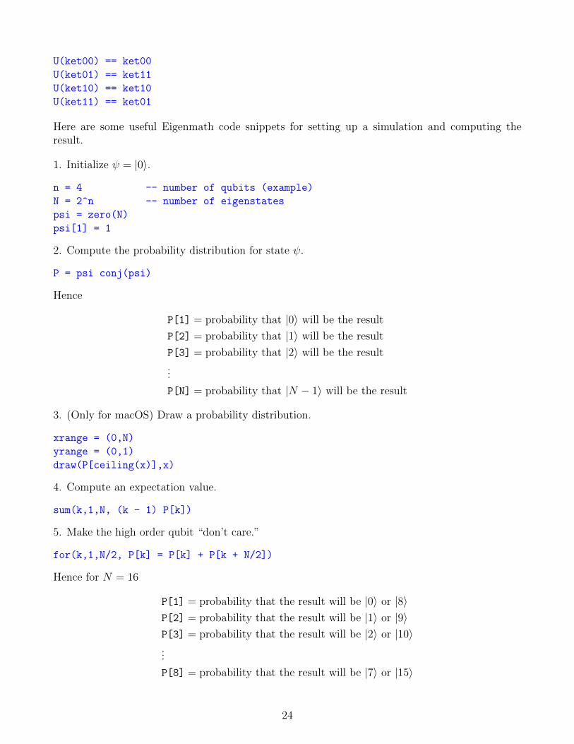
U(ket00) == ket00
U(ket01) == ket11
U(ket10) == ket10
U(ket11) == ket01
Here are some useful Eigenmath code snippets for setting up a simulation and computing theresult.
1. Initialize ψ = |0〉.
n = 4 -- number of qubits (example)
N = 2^n -- number of eigenstates
psi = zero(N)
psi[1] = 1
2. Compute the probability distribution for state ψ.
P = psi conj(psi)
Hence
P[1] = probability that |0〉 will be the result
P[2] = probability that |1〉 will be the result
P[3] = probability that |2〉 will be the result
...
P[N] = probability that |N − 1〉 will be the result
3. (Only for macOS) Draw a probability distribution.
xrange = (0,N)
yrange = (0,1)
draw(P[ceiling(x)],x)
4. Compute an expectation value.
sum(k,1,N, (k - 1) P[k])
5. Make the high order qubit “don’t care.”
for(k,1,N/2, P[k] = P[k] + P[k + N/2])
Hence for N = 16
P[1] = probability that the result will be |0〉 or |8〉P[2] = probability that the result will be |1〉 or |9〉P[3] = probability that the result will be |2〉 or |10〉...
P[8] = probability that the result will be |7〉 or |15〉
24
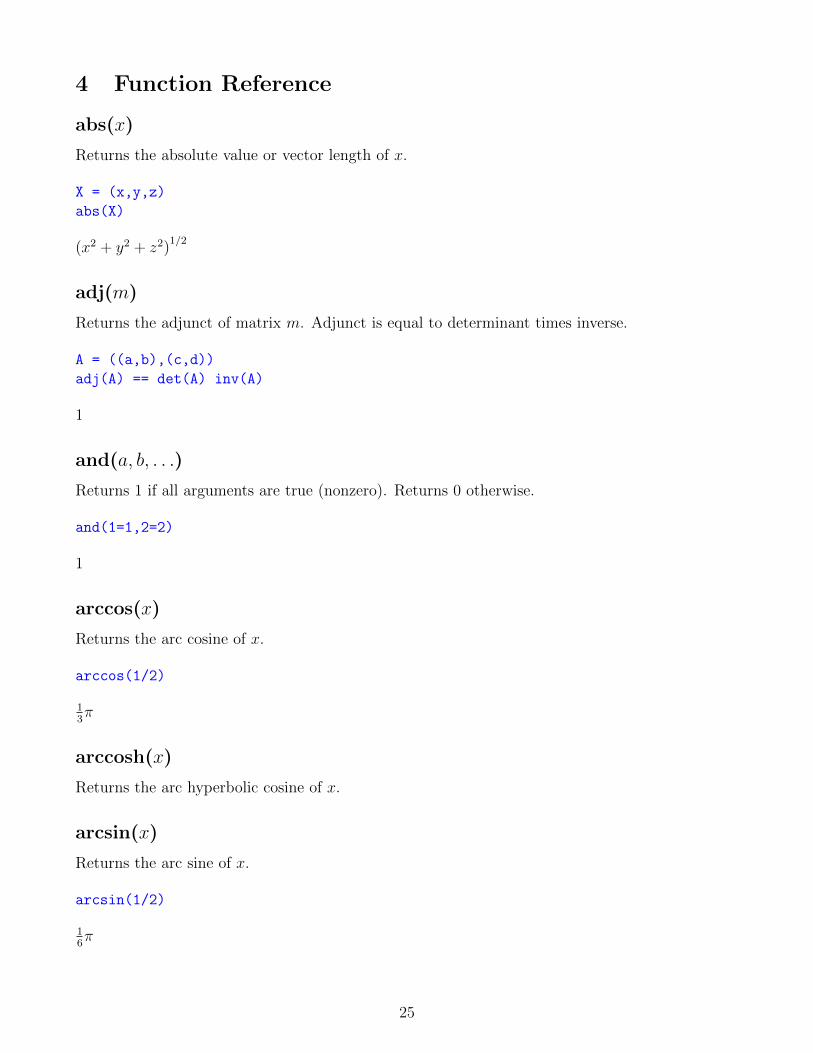
4 Function Reference
abs(x)
Returns the absolute value or vector length of x.
X = (x,y,z)
abs(X)
(x2 + y2 + z2)1/2
adj(m)
Returns the adjunct of matrix m. Adjunct is equal to determinant times inverse.
A = ((a,b),(c,d))
adj(A) == det(A) inv(A)
1
and(a, b, . . .)
Returns 1 if all arguments are true (nonzero). Returns 0 otherwise.
and(1=1,2=2)
1
arccos(x)
Returns the arc cosine of x.
arccos(1/2)
13π
arccosh(x)
Returns the arc hyperbolic cosine of x.
arcsin(x)
Returns the arc sine of x.
arcsin(1/2)
16π
25
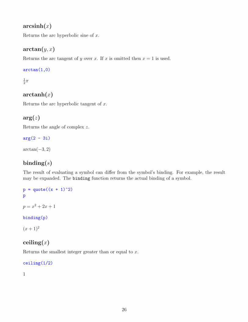
arcsinh(x)
Returns the arc hyperbolic sine of x.
arctan(y, x)
Returns the arc tangent of y over x. If x is omitted then x = 1 is used.
arctan(1,0)
12π
arctanh(x)
Returns the arc hyperbolic tangent of x.
arg(z)
Returns the angle of complex z.
arg(2 - 3i)
arctan(−3, 2)
binding(s)
The result of evaluating a symbol can differ from the symbol’s binding. For example, the resultmay be expanded. The binding function returns the actual binding of a symbol.
p = quote((x + 1)^2)
p
p = x2 + 2x+ 1
binding(p)
(x+ 1)2
ceiling(x)
Returns the smallest integer greater than or equal to x.
ceiling(1/2)
1
26
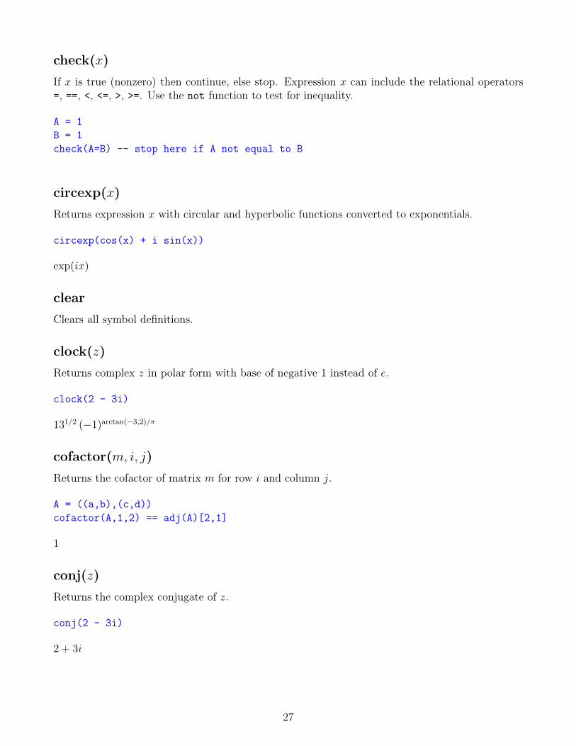
check(x)
If x is true (nonzero) then continue, else stop. Expression x can include the relational operators=, ==, <, <=, >, >=. Use the not function to test for inequality.
A = 1
B = 1
check(A=B) -- stop here if A not equal to B
circexp(x)
Returns expression x with circular and hyperbolic functions converted to exponentials.
circexp(cos(x) + i sin(x))
exp(ix)
clear
Clears all symbol definitions.
clock(z)
Returns complex z in polar form with base of negative 1 instead of e.
clock(2 - 3i)
131/2 (−1)arctan(−3,2)/π
cofactor(m, i, j)
Returns the cofactor of matrix m for row i and column j.
A = ((a,b),(c,d))
cofactor(A,1,2) == adj(A)[2,1]
1
conj(z)
Returns the complex conjugate of z.
conj(2 - 3i)
2 + 3i
27
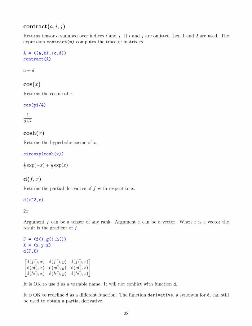
contract(a, i, j)
Returns tensor a summed over indices i and j. If i and j are omitted then 1 and 2 are used. Theexpression contract(m) computes the trace of matrix m.
A = ((a,b),(c,d))
contract(A)
a+ d
cos(x)
Returns the cosine of x.
cos(pi/4)
1
21/2
cosh(x)
Returns the hyperbolic cosine of x.
circexp(cosh(x))
12
exp(−x) + 12
exp(x)
d(f, x)
Returns the partial derivative of f with respect to x.
d(x^2,x)
2x
Argument f can be a tensor of any rank. Argument x can be a vector. When x is a vector theresult is the gradient of f .
F = (f(),g(),h())
X = (x,y,z)
d(F,X)d(f(), x) d(f(), y) d(f(), z)d(g(), x) d(g(), y) d(g(), z)d(h(), x) d(h(), y) d(h(), z)
It is OK to use d as a variable name. It will not conflict with function d.
It is OK to redefine d as a different function. The function derivative, a synonym for d, can stillbe used to obtain a partial derivative.
28

defint(f, x, a, b)
Returns the definite integral of f with respect to x evaluated from a to b. The argument list canbe extended for multiple integrals as shown in the following example.
f = (1 + cos(theta)^2) sin(theta)
defint(f, theta, 0, pi, phi, 0, 2pi) -- integrate over theta then over phi
163π
denominator(x)
Returns the denominator of expression x.
denominator(a/b)
b
det(m)
Returns the determinant of matrix m.
A = ((a,b),(c,d))
det(A)
ad− bc
dim(a, n)
Returns the dimension of the nth index of tensor a. Index numbering starts with 1.
A = ((1,2),(3,4),(5,6))
dim(A,1)
3
do(a, b, . . .)
Evaluates each argument from left to right. Returns the result of the final argument.
do(A=1,B=2,A+B)
3
29
dot(a, b, . . .)
Returns the dot product of vectors, matrices, and tensors. Also known as the matrix product.
-- solve for X in AX=B
A = ((1,2),(3,4))
B = (5,6)
X = dot(inv(A),B)
X[−492
]
draw(f, x)
(Only for macOS) Draws a graph of f(x). Drawing ranges can be set with xrange and yrange.
xrange = (0,1)
yrange = (0,1)
draw(x^2,x)
eval(f, x, a)
Returns expression f evaluated at x equals a. The argument list can be extended for multivariateexpressions. For example, eval(f,x,a,y,b) is equivalent to eval(eval(f,x,a),y,b).
eval(x + y,x,a,y,b)
a+ b
exp(x)
Returns the exponential of x.
exp(i pi)
−1
expcos(z)
Returns the cosine of z in exponential form.
expcos(z)
12
exp(iz) + 12
exp(−iz)
30
expcosh(z)
Returns the hyperbolic cosine of z in exponential form.
expcosh(z)
12
exp(−z) + 12
exp(z)
expsin(z)
Returns the sine of z in exponential form.
expsin(z)
−12i exp(iz) + 1
2i exp(−iz)
expsinh(z)
Returns the hyperbolic sine of z in exponential form.
expsinh(z)
−12
exp(−z) + 12
exp(z)
exptan(z)
Returns the tangent of z in exponential form.
exptan(z)
i
exp(2iz) + 1− i exp(2iz)
exp(2iz) + 1
exptanh(z)
Returns the hyperbolic tangent of z in exponential form.
exptanh(z)
− 1
exp(2z) + 1+
exp(2z)
exp(2z) + 1
factorial(n)
Returns the factorial of n. The expression n! can also be used.
20!
2432902008176640000
31
float(x)
Returns expression x with rational numbers and integers converted to floating point values. Thesymbol pi and the natural number are also converted.
float(212^17)
3.52947× 1039
floor(x)
Returns the largest integer less than or equal to x.
floor(1/2)
0
for(i, j, k, a, b, . . .)
For i equals j through k evaluate a, b, etc.
for(k,1,3,A=k,print(A))
A = 1A = 2A = 3
Note: The original value of i is restored after for completes. If symbol i is used for index variablei then the imaginary unit is overridden in the scope of for.
hadamard(a, b, . . .)
Returns the Hadamard (element-wise) product.
X = (a,b,c)
hadamard(X,X)a2b2c2
i
Symbol i is initialized to the imaginary unit√−1.
exp(i pi)
−1
Note: It is OK to clear or redefine i and use the symbol for something else.
32
imag(z)
Returns the imaginary part of complex z.
imag(2 - 3i)
−3
inner(a, b, . . .)
Returns the inner product of vectors, matrices, and tensors. Also known as the matrix product.
A = ((a,b),(c,d))
B = (x,y)
inner(A,B)[ax+ bycx+ dy
]Note: inner and dot are the same function.
integral(f, x)
Returns the integral of f with respect to x.
integral(x^2,x)
13x3
inv(m)
Returns the inverse of matrix m.
A = ((1,2),(3,4))
inv(A)[−2 132−1
2
]
j
Set j=sqrt(-1) to use j for the imaginary unit instead of i.
j = sqrt(-1)
1/sqrt(-1)
−j
33
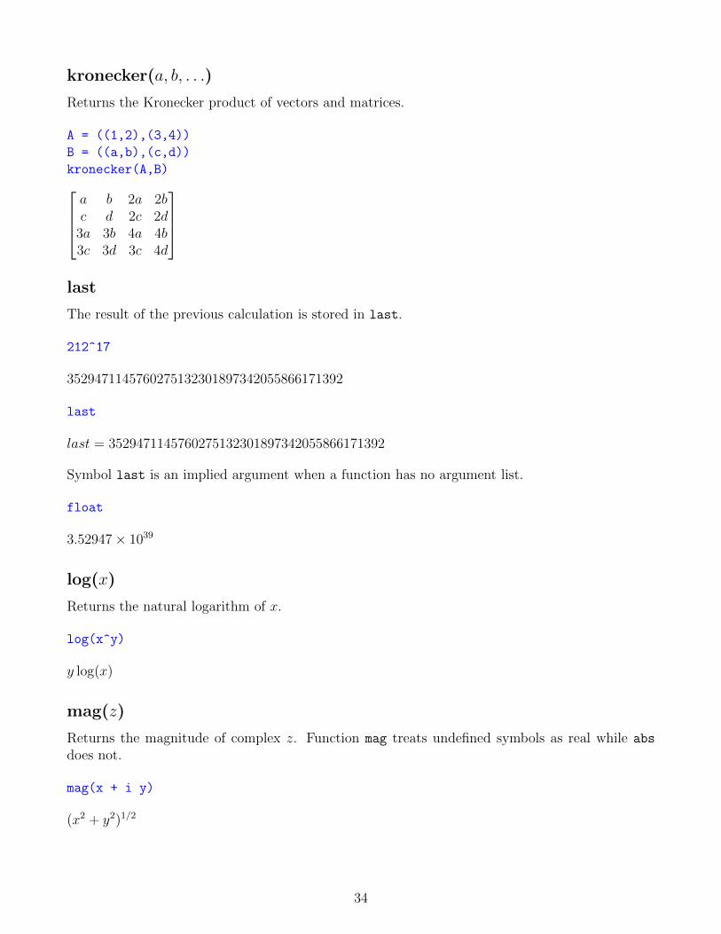
kronecker(a, b, . . .)
Returns the Kronecker product of vectors and matrices.
A = ((1,2),(3,4))
B = ((a,b),(c,d))
kronecker(A,B)a b 2a 2bc d 2c 2d
3a 3b 4a 4b3c 3d 3c 4d
last
The result of the previous calculation is stored in last.
212^17
3529471145760275132301897342055866171392
last
last = 3529471145760275132301897342055866171392
Symbol last is an implied argument when a function has no argument list.
float
3.52947× 1039
log(x)
Returns the natural logarithm of x.
log(x^y)
y log(x)
mag(z)
Returns the magnitude of complex z. Function mag treats undefined symbols as real while abs
does not.
mag(x + i y)
(x2 + y2)1/2
34
minor(m, i, j)
Returns the minor of matrix m for row i and column j.
A = ((1,2,3),(4,5,6),(7,8,9))
minor(A,1,1) == det(minormatrix(A,1,1))
1
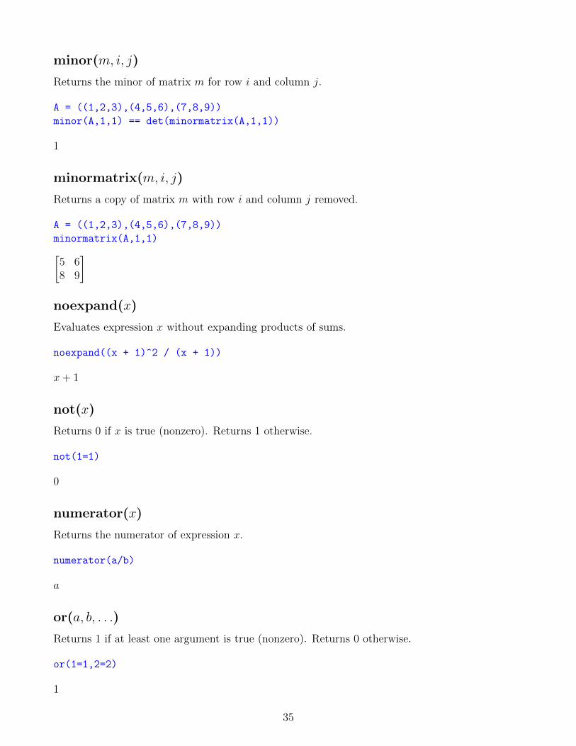
minormatrix(m, i, j)
Returns a copy of matrix m with row i and column j removed.
A = ((1,2,3),(4,5,6),(7,8,9))
minormatrix(A,1,1)[5 68 9
]
noexpand(x)
Evaluates expression x without expanding products of sums.
noexpand((x + 1)^2 / (x + 1))
x+ 1
not(x)
Returns 0 if x is true (nonzero). Returns 1 otherwise.
not(1=1)
0
numerator(x)
Returns the numerator of expression x.
numerator(a/b)
a
or(a, b, . . .)
Returns 1 if at least one argument is true (nonzero). Returns 0 otherwise.
or(1=1,2=2)
1
35
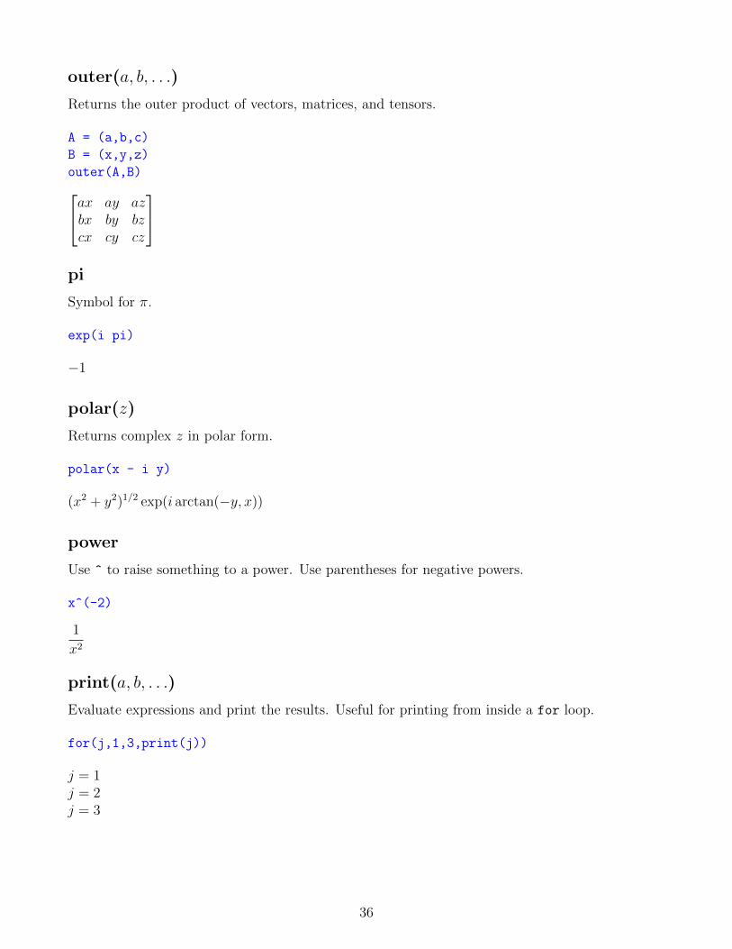
outer(a, b, . . .)
Returns the outer product of vectors, matrices, and tensors.
A = (a,b,c)
B = (x,y,z)
outer(A,B)ax ay azbx by bzcx cy cz
pi
Symbol for π.
exp(i pi)
−1
polar(z)
Returns complex z in polar form.
polar(x - i y)
(x2 + y2)1/2 exp(i arctan(−y, x))
power
Use ^ to raise something to a power. Use parentheses for negative powers.
x^(-2)
1
x2
print(a, b, . . .)
Evaluate expressions and print the results. Useful for printing from inside a for loop.
for(j,1,3,print(j))
j = 1j = 2j = 3
36
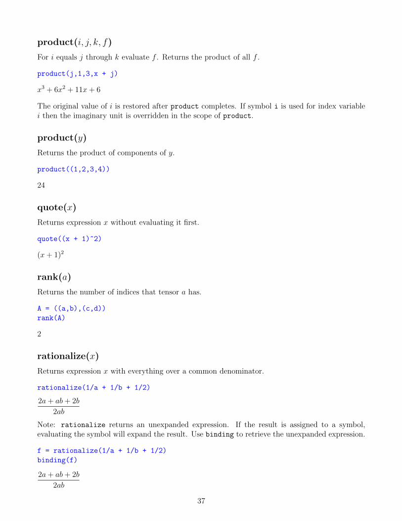
product(i, j, k, f)
For i equals j through k evaluate f . Returns the product of all f .
product(j,1,3,x + j)
x3 + 6x2 + 11x+ 6
The original value of i is restored after product completes. If symbol i is used for index variablei then the imaginary unit is overridden in the scope of product.
product(y)
Returns the product of components of y.
product((1,2,3,4))
24
quote(x)
Returns expression x without evaluating it first.
quote((x + 1)^2)
(x+ 1)2
rank(a)
Returns the number of indices that tensor a has.
A = ((a,b),(c,d))
rank(A)
2
rationalize(x)
Returns expression x with everything over a common denominator.
rationalize(1/a + 1/b + 1/2)
2a+ ab+ 2b
2ab
Note: rationalize returns an unexpanded expression. If the result is assigned to a symbol,evaluating the symbol will expand the result. Use binding to retrieve the unexpanded expression.
f = rationalize(1/a + 1/b + 1/2)
binding(f)
2a+ ab+ 2b
2ab
37
real(z)
Returns the real part of complex z.
real(2 - 3i)
2
rect(z)
Returns complex z in rectangular form.
rect(exp(i x))
cos(x) + i sin(x)
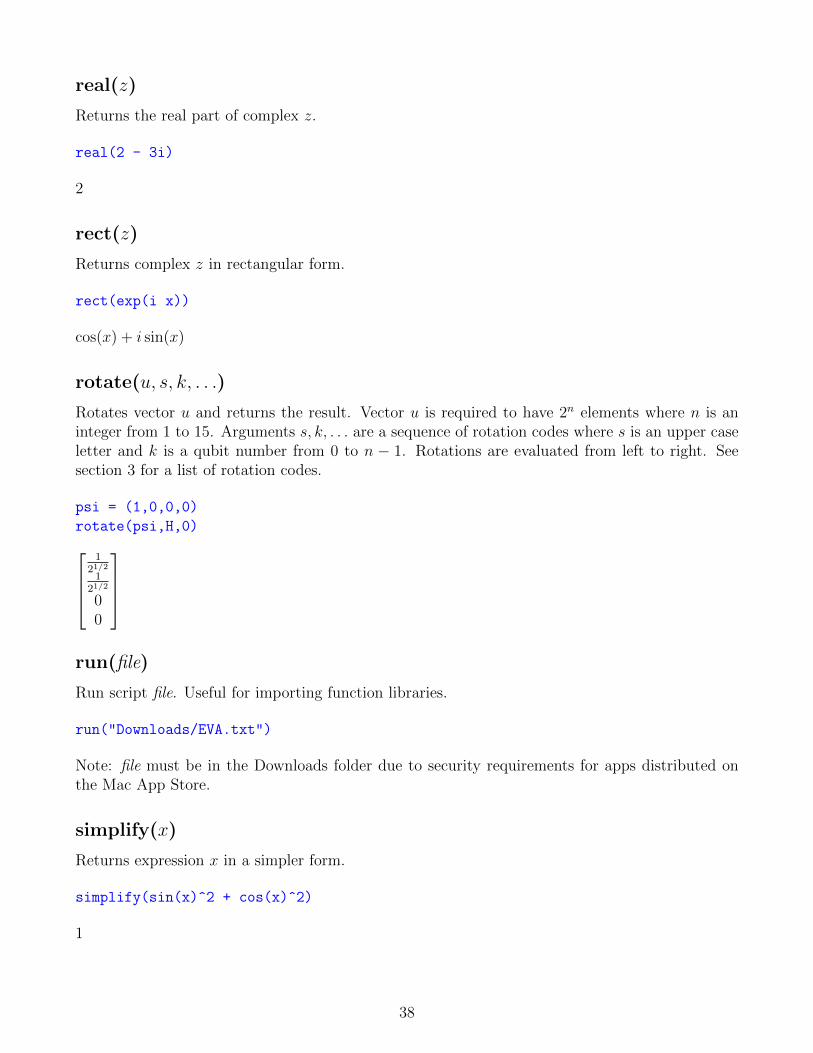
rotate(u, s, k, . . .)
Rotates vector u and returns the result. Vector u is required to have 2n elements where n is aninteger from 1 to 15. Arguments s, k, . . . are a sequence of rotation codes where s is an upper caseletter and k is a qubit number from 0 to n − 1. Rotations are evaluated from left to right. Seesection 3 for a list of rotation codes.
psi = (1,0,0,0)
rotate(psi,H,0)1
21/21
21/2
00
run(file)
Run script file. Useful for importing function libraries.
run("Downloads/EVA.txt")
Note: file must be in the Downloads folder due to security requirements for apps distributed onthe Mac App Store.
simplify(x)
Returns expression x in a simpler form.
simplify(sin(x)^2 + cos(x)^2)
1
38
sin(x)
Returns the sine of x.
sin(pi/4)
1
21/2
sinh(x)
Returns the hyperbolic sine of x.
circexp(sinh(x))
−12
exp(−x) + 12
exp(x)
sqrt(x)
Returns the square root of x.
sqrt(10!)
720 71/2
stop
In a script, it does what it says.
sum(i, j, k, f)
For i equals j through k evaluate f . Returns the sum of all f .
sum(j,1,5,x^j)
x5 + x4 + x3 + x2 + x
The original value of i is restored after sum completes. If symbol i is used for index variable i thenthe imaginary unit is overridden in the scope of sum.
sum(y)
Returns the sum of components of y.
sum((1,2,3,4))
10
39
tan(x)
Returns the tangent of x.
simplify(tan(x) - sin(x)/cos(x))
0
tanh(x)
Returns the hyperbolic tangent of x.
circexp(tanh(x))
− 1
exp(2x) + 1+
exp(2x)
exp(2x) + 1
test(a, b, c, d, . . .)
If argument a is true (nonzero) then b is returned, else if c is true then d is returned, etc. If thenumber of arguments is odd then the final argument is returned if all else fails. Expressions caninclude the relational operators =, ==, <, <=, >, >=. Use the not function to test for inequality.(The equality operator == is available for contexts in which = is the assignment operator.)
A = 1
B = 1
test(A=B,"yes","no")
yes
trace
Set trace=1 in a script to print the script as it is evaluated. Useful for debugging.
trace = 1
Note: The contract function is used to obtain the trace of a matrix.
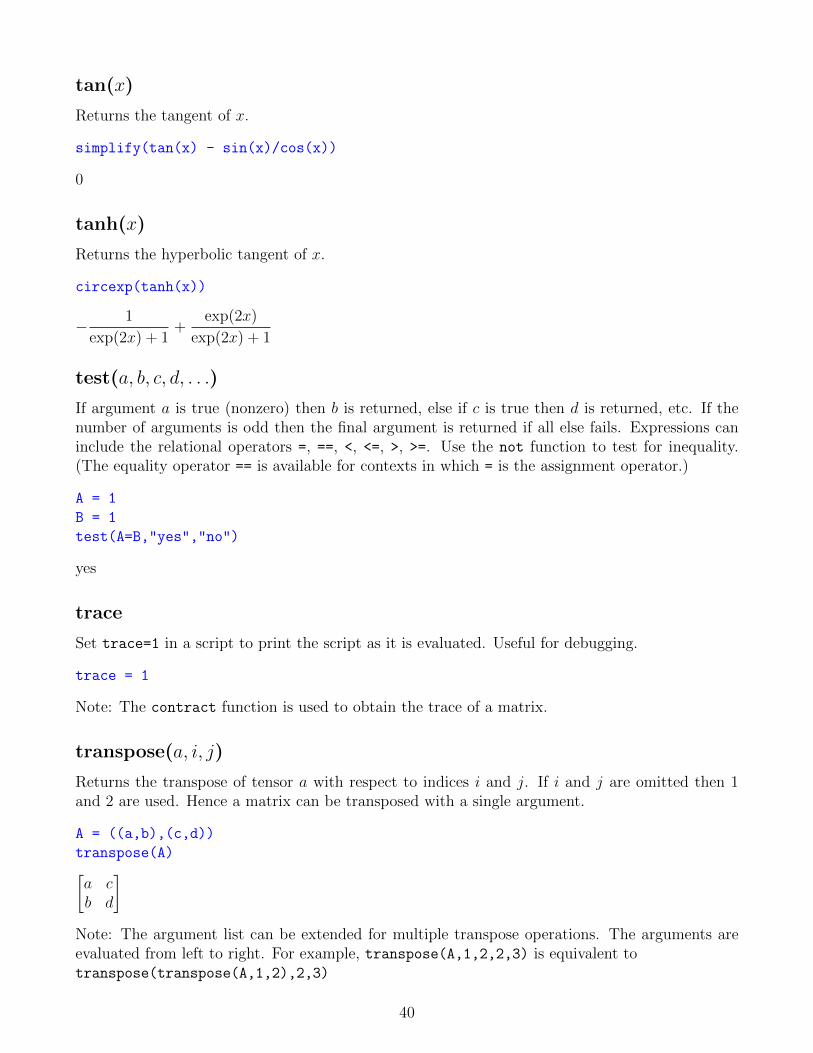
transpose(a, i, j)
Returns the transpose of tensor a with respect to indices i and j. If i and j are omitted then 1and 2 are used. Hence a matrix can be transposed with a single argument.
A = ((a,b),(c,d))
transpose(A)[a cb d
]Note: The argument list can be extended for multiple transpose operations. The arguments areevaluated from left to right. For example, transpose(A,1,2,2,3) is equivalent totranspose(transpose(A,1,2),2,3)
40
unit(n)
Returns an n by n identity matrix.
unit(3)1 0 00 1 00 0 1
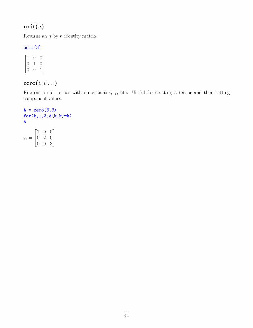
zero(i, j, . . .)
Returns a null tensor with dimensions i, j, etc. Useful for creating a tensor and then settingcomponent values.
A = zero(3,3)
for(k,1,3,A[k,k]=k)
A
A =
1 0 00 2 00 0 3
41
5 Tricks
1. In a script, line breaking is allowed provided the line breaks occur immediately after opera-tors. The scanner will automatically go to the next line after an operator.
2. Setting trace=1 in a script causes each line to be printed just before it is evaluated. This isuseful for debugging.
3. The last result is stored in the symbol last.
4. Use contract(A) to get the mathematical trace of matrix A.
5. Use binding(s) to get the unevaluated binding of symbol s.
6. Use s=quote(s) to clear symbol s.
7. Use float(pi) to get the floating point value of π. Set pi=float(pi) to evaluate expressionswith a numerical value for π. Set pi=quote(pi) to make π symbolic again.
8. Assign strings to unit names so they are printed normally. For example, setting meter="meter"causes the symbol meter to be printed as meter instead of meter.
9. Use expsin and expcos instead of sin and cos. Trigonometric simplifications occur auto-matically when exponentials are used.
10. Use A==B or A-B==0 to test for equality of A and B. The equality operator == uses a crossmultiply algorithm to eliminate denominators. Hence == can typically determine equalityeven when the unsimplified result of A−B is nonzero. Note: Equality tests involving floatingpoint numbers can be problematic due to roundoff error.
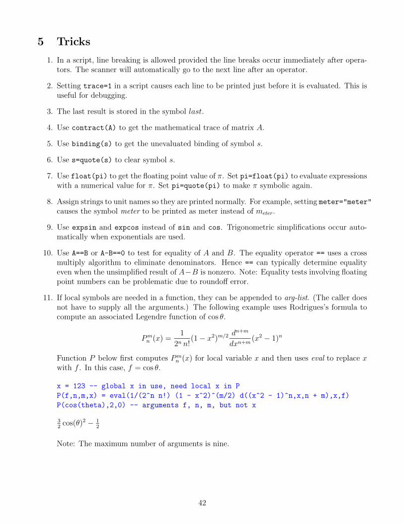
11. If local symbols are needed in a function, they can be appended to arg-list. (The caller doesnot have to supply all the arguments.) The following example uses Rodrigues’s formula tocompute an associated Legendre function of cos θ.
Pmn (x) =
1
2n n!(1− x2)m/2 d
n+m
dxn+m(x2 − 1)n
Function P below first computes Pmn (x) for local variable x and then uses eval to replace x
with f . In this case, f = cos θ.
x = 123 -- global x in use, need local x in P
P(f,n,m,x) = eval(1/(2^n n!) (1 - x^2)^(m/2) d((x^2 - 1)^n,x,n + m),x,f)
P(cos(theta),2,0) -- arguments f, n, m, but not x
32
cos(θ)2 − 12
Note: The maximum number of arguments is nine.
42