eigenfunctions on the surface of a spherekglasner/math456/spherical... · 2019-02-13 ·...
TRANSCRIPT

Eigenfunctions on the surface of a sphere
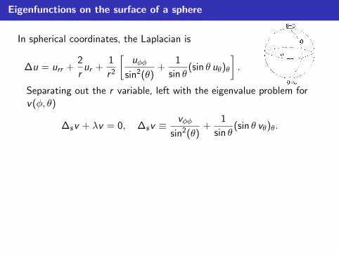
In spherical coordinates, the Laplacian is
∆u = urr +2
rur +
1
r2
[uφφ
sin2(θ)+
1
sin θ(sin θ uθ)θ
].
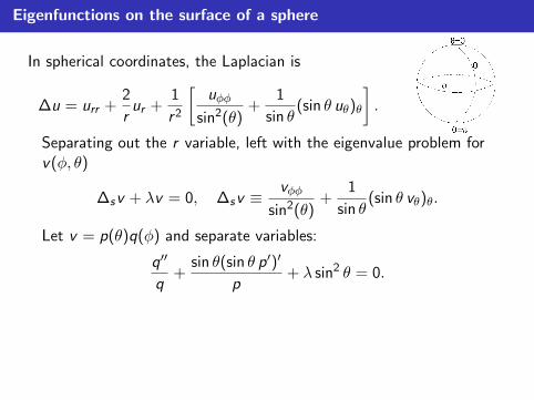
Separating out the r variable, left with the eigenvalue problem forv(φ, θ)
∆sv + λv = 0, ∆sv ≡vφφ
sin2(θ)+
1
sin θ(sin θ vθ)θ.
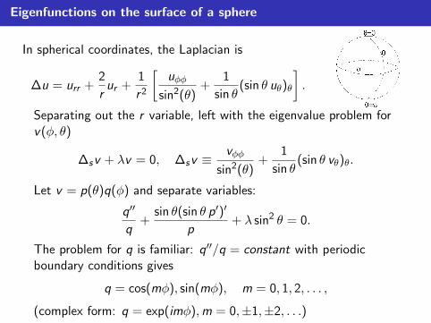
Let v = p(θ)q(φ) and separate variables:
q′′
q+
sin θ(sin θ p′)′
p+ λ sin2 θ = 0.
The problem for q is familiar: q′′/q = constant with periodicboundary conditions gives
q = cos(mφ), sin(mφ), m = 0, 1, 2, . . . ,
(complex form: q = exp(imφ),m = 0,±1,±2, . . .)
Eigenfunctions on the surface of a sphere
In spherical coordinates, the Laplacian is
∆u = urr +2
rur +
1
r2
[uφφ
sin2(θ)+
1
sin θ(sin θ uθ)θ
].
Separating out the r variable, left with the eigenvalue problem forv(φ, θ)
∆sv + λv = 0, ∆sv ≡vφφ
sin2(θ)+
1
sin θ(sin θ vθ)θ.
Let v = p(θ)q(φ) and separate variables:
q′′
q+
sin θ(sin θ p′)′
p+ λ sin2 θ = 0.
The problem for q is familiar: q′′/q = constant with periodicboundary conditions gives
q = cos(mφ), sin(mφ), m = 0, 1, 2, . . . ,
(complex form: q = exp(imφ),m = 0,±1,±2, . . .)
Eigenfunctions on the surface of a sphere, cont.
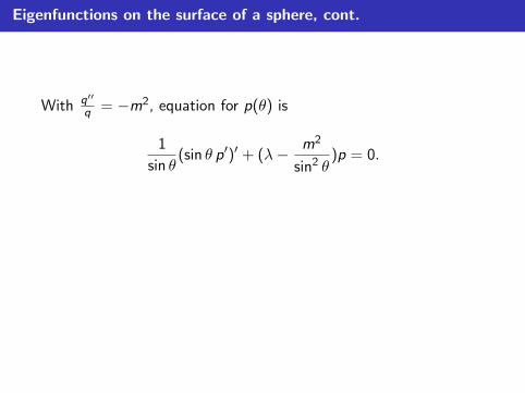
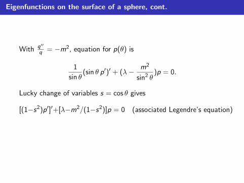
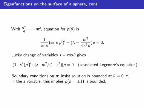
With q′′
q = −m2, equation for p(θ) is
1
sin θ(sin θ p′)′ + (λ− m2
sin2 θ)p = 0.
Lucky change of variables s = cos θ gives
[(1−s2)p′]′+[λ−m2/(1−s2)]p = 0 (associated Legendre’s equation)
Boundary conditions on p: insist solution is bounded at θ = 0, π.In the s variable, this implies p(s = ±1) is bounded.
Eigenfunctions on the surface of a sphere, cont.
With q′′
q = −m2, equation for p(θ) is
1
sin θ(sin θ p′)′ + (λ− m2
sin2 θ)p = 0.
Lucky change of variables s = cos θ gives
[(1−s2)p′]′+[λ−m2/(1−s2)]p = 0 (associated Legendre’s equation)
Boundary conditions on p: insist solution is bounded at θ = 0, π.In the s variable, this implies p(s = ±1) is bounded.
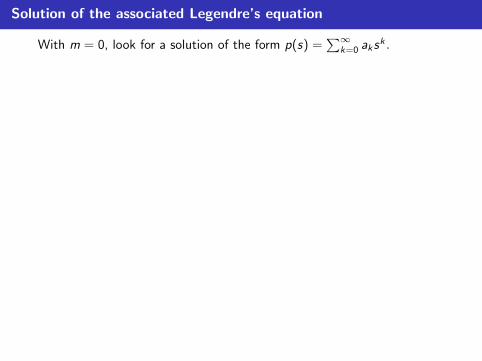
Solution of the associated Legendre’s equation
With m = 0, look for a solution of the form p(s) =∑∞
k=0 aksk .
Substituting into the equation∞∑k=2
(k + 2)(k + 1)ak+2sk −
∞∑k=0
(k2 + k − λ)aksk = 0.
Equating coefficients of sk leads to the recursion relation
ak+2 = akk(k + 1)− λ
(k + 2)(k + 1).
If λ = l(l + 1) for l = 0, 1, 2, 3, ... series solution has zerocoefficients for k > l ; yields famous Legendre polynomials Pl(s):
P0 = 1, P1 = s, P2 =1
2(3s2 − 1), . . .
If λ 6= l(l + 1) for positive integer l , power series has radius ofconvergence = 1, and thus series diverges at s = ±1.
For m > 0: remarkable formula
p(s) = Pml (s) ≡ (1− s2)m/2
dm
dsmPl(s).
This requires m ≤ l to get nonzero answer.

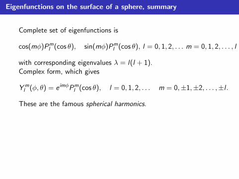
Eigenfunctions on the surface of a sphere, summary
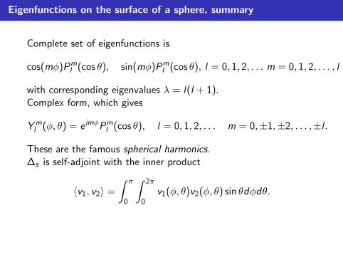
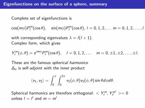
Complete set of eigenfunctions is
cos(mφ)Pml (cos θ), sin(mφ)Pm
l (cos θ), l = 0, 1, 2, . . . m = 0, 1, 2, . . . , l
with corresponding eigenvalues λ = l(l + 1).
Complex form, which gives
Yml (φ, θ) = e imφPm
l (cos θ), l = 0, 1, 2, . . . m = 0,±1,±2, . . . ,±l .
These are the famous spherical harmonics.∆s is self-adjoint with the inner product
〈v1, v2〉 =
∫ π
0
∫ 2π
0v1(φ, θ)v2(φ, θ) sin θdφdθ.
Spherical harmonics are therefore orthogonal: < Yml ,Y
m′l ′ >= 0
unless l = l ′ and m = m′
Eigenfunctions on the surface of a sphere, summary
Complete set of eigenfunctions is
cos(mφ)Pml (cos θ), sin(mφ)Pm
l (cos θ), l = 0, 1, 2, . . . m = 0, 1, 2, . . . , l
with corresponding eigenvalues λ = l(l + 1).Complex form, which gives
Yml (φ, θ) = e imφPm
l (cos θ), l = 0, 1, 2, . . . m = 0,±1,±2, . . . ,±l .
These are the famous spherical harmonics.
∆s is self-adjoint with the inner product
〈v1, v2〉 =
∫ π
0
∫ 2π
0v1(φ, θ)v2(φ, θ) sin θdφdθ.
Spherical harmonics are therefore orthogonal: < Yml ,Y
m′l ′ >= 0
unless l = l ′ and m = m′
Eigenfunctions on the surface of a sphere, summary
Complete set of eigenfunctions is
cos(mφ)Pml (cos θ), sin(mφ)Pm
l (cos θ), l = 0, 1, 2, . . . m = 0, 1, 2, . . . , l
with corresponding eigenvalues λ = l(l + 1).Complex form, which gives
Yml (φ, θ) = e imφPm
l (cos θ), l = 0, 1, 2, . . . m = 0,±1,±2, . . . ,±l .
These are the famous spherical harmonics.∆s is self-adjoint with the inner product
〈v1, v2〉 =
∫ π
0
∫ 2π
0v1(φ, θ)v2(φ, θ) sin θdφdθ.
Spherical harmonics are therefore orthogonal: < Yml ,Y
m′l ′ >= 0
unless l = l ′ and m = m′
Eigenfunctions on the surface of a sphere, summary
Complete set of eigenfunctions is
cos(mφ)Pml (cos θ), sin(mφ)Pm
l (cos θ), l = 0, 1, 2, . . . m = 0, 1, 2, . . . , l
with corresponding eigenvalues λ = l(l + 1).Complex form, which gives
Yml (φ, θ) = e imφPm
l (cos θ), l = 0, 1, 2, . . . m = 0,±1,±2, . . . ,±l .
These are the famous spherical harmonics.∆s is self-adjoint with the inner product
〈v1, v2〉 =
∫ π
0
∫ 2π
0v1(φ, θ)v2(φ, θ) sin θdφdθ.
Spherical harmonics are therefore orthogonal: < Yml ,Y
m′l ′ >= 0
unless l = l ′ and m = m′
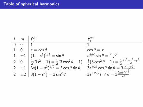
Table of spherical harmonics
l m P|m|l Ym
l
0 0 1 11 0 s = cos θ cos θ = z
1 ±1 (1− s2)1/2 = sin θ e±iφ sin θ = x±iyr
2 0 12(3s2 − 1) = 1
2(3 cos2 θ − 1) 12(3 cos2 θ − 1) = 1
22z2−x2−y2
r2
2 ±1 3s(1− s2)1/2 = 3 cos θ sin θ 3e±iφ cos θ sin θ = 3 (x±iy)zr2
2 ±2 3(1− s2) = 3 sin2 θ 3e±2iφ sin2 θ = 3 (x±iy)2r2
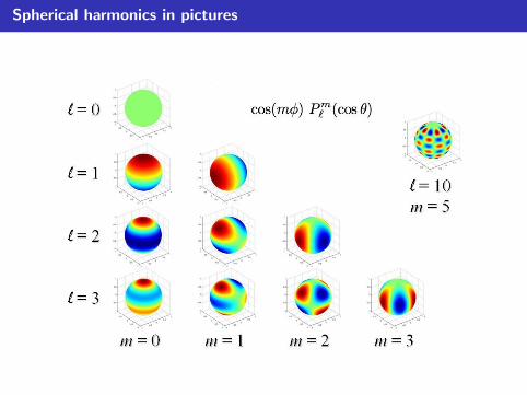
Spherical harmonics in pictures

Example: solving Laplace equation inside sphere
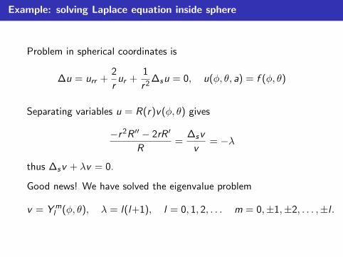
Problem in spherical coordinates is
∆u = urr +2
rur +
1
r2∆su = 0, u(φ, θ, a) = f (φ, θ)
Separating variables u = R(r)v(φ, θ) gives
−r2R ′′ − 2rR ′
R=
∆sv
v= −λ
thus ∆sv + λv = 0.
Good news! We have solved the eigenvalue problem
v = Yml (φ, θ), λ = l(l+1), l = 0, 1, 2, . . . m = 0,±1,±2, . . . ,±l .

Example: solving Laplace equation inside sphere
Problem in spherical coordinates is
∆u = urr +2
rur +
1
r2∆su = 0, u(φ, θ, a) = f (φ, θ)
Separating variables u = R(r)v(φ, θ) gives
−r2R ′′ − 2rR ′
R=
∆sv
v= −λ
thus ∆sv + λv = 0.
Good news! We have solved the eigenvalue problem
v = Yml (φ, θ), λ = l(l+1), l = 0, 1, 2, . . . m = 0,±1,±2, . . . ,±l .

Example: solving Laplace equation inside sphere, cont.
Now for R equation
r2R ′′ + 2rR ′ − l(l + 1)R = 0,
which is an Euler equation with solutions R = rα.
Substituting gives
α(α− 1) + 2α− l(l + 1) = (α− l)(α + l + 1) = 0
Thus α = l or α = −l − 1. (reject latter)
Now put it all together as superposition:
u =∞∑l=0
l∑m=−l
AlmrlYm
l (φ, θ), Alm are potentially complex.
Use orthogonality to find coefficients:
f (φ, θ) =∞∑l=0
l∑m=−l
AlmalYm
l (φ, θ)
so that
Alm =1
al〈f ,Ym
l 〉〈Ym
l ,Yml 〉
, 〈v1, v2〉 =
∫ π
0
∫ 2π
0
v1(φ, θ)v2(θ, φ) sin θdφdθ.

Example: solving Laplace equation inside sphere, cont.
Now for R equation
r2R ′′ + 2rR ′ − l(l + 1)R = 0,
which is an Euler equation with solutions R = rα. Substituting gives
α(α− 1) + 2α− l(l + 1) = (α− l)(α + l + 1) = 0
Thus α = l or α = −l − 1. (reject latter)
Now put it all together as superposition:
u =∞∑l=0
l∑m=−l
AlmrlYm
l (φ, θ), Alm are potentially complex.
Use orthogonality to find coefficients:
f (φ, θ) =∞∑l=0
l∑m=−l
AlmalYm
l (φ, θ)
so that
Alm =1
al〈f ,Ym
l 〉〈Ym
l ,Yml 〉
, 〈v1, v2〉 =
∫ π
0
∫ 2π
0
v1(φ, θ)v2(θ, φ) sin θdφdθ.

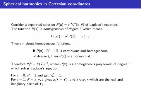
Spherical harmonics in Cartesian coordinates
Consider a separated solution P(x) = r lY ml (φ, θ) of Laplace’s equation.
The function P(x) is homogeneous of degree l , which means
P(αx) = αlP(x), α > 0.
Theorem about homogeneous functions:
If P(x) : Rn → R is continuous and homogeneous,
of degree l , then P(x) is a polynomial.
Therefore Y ml = P(x)/r l , where P(x) is a homogeneous polynomial of degree l
which solves Laplace’s equation.
For l = 0, P = 1 and get Y 00 = 1.
For l = 1, P = x , y , z gives z/r = Y 01 , and x/r ,y/r which are the real and
imaginary parts of Y 11 .