Brightness, Lightness, and Specifying Color in High-Dynamic-Range Scenes and Images

Mark D. Fairchild and Ping-Hsu Chen*

Munsell Color Science Laboratory, Chester F. Carlson Center for Imaging Science, Rochester Institute of Technology, Rochester, NY, USA 14623-5604

ABSTRACT

Traditional color spaces have been widely used in a variety of applications including digital color imaging, color image quality, and color management. These spaces, however, were designed for the domain of color stimuli typically encountered with reflecting objects and image displays of such objects. This means the domain of stimuli with luminance levels from slightly above zero to that of a perfect diffuse white (or display white point). This limits the applicability of such spaces to color problems in HDR imaging. This is caused by their hard intercepts at zero luminance/lightness and by their uncertain applicability for colors brighter than diffuse white. To address HDR applications, two new color spaces were recently proposed, hdr-CIELAB and hdr-IPT. They are based on replacing the power-function nonlinearities in CIELAB and IPT with more physiologically plausible hyperbolic functions optimized to most closely simulate the original color spaces in the diffuse reflecting color domain. This paper presents the formulation of the new models, evaluations using Munsell data in comparison with CIELAB, IPT, and CIECAM02, two sets of lightness-scaling data above diffuse white, and various possible formulations of hdr-CIELAB and hdr-IPT to predict the visual results.

Keywords: HDR, Color Spaces, Color Differences, Image Quality, Lightness, Color Appearance

1. INTRODUCTION Traditional color spaces such as the CIE 1976 L*a*b* Color Space, CIELAB, and the IPT space optimized for hue linearity have been widely and successfully used in a variety of applications including digital color imaging, color image quality, and color management. These spaces, however, were designed for the domain of color stimuli typically encountered with reflecting objects and image displays of such objects. More specifically, this means stimuli with luminance levels from slightly above zero to that of a perfect diffuse white (or display white point), or dynamic ranges of approximately 100:1. This limits the applicability of both of these spaces to color and image quality problems in high-dynamic-range (HDR) imaging. This is caused by their hard intercepts at zero luminance/lightness and by their uncertain applicability for colors brighter than diffuse white. To address these HDR questions, two newly formulated color spaces were recently proposed for further testing and refinement, hdr-CIELAB and hdr-IPT.1 They are based on replacing the power-function nonlinearities in CIELAB and IPT with a more physiologically plausible hyperbolic functions, based on the Michaelis-Menten equation, optimized to most closely simulate the original color spaces in the diffuse reflecting color domain.

In addition, experiments have been completed to scale lightness and lightness differences in the range well above the lightness of diffuse white.2 Overall a range of CIELAB lightness values from 7 to 183 was investigated. The results indicated that the existing L* and CIEDE2000-weighting functions approximately predict the trends, but do not well fit the visual data. Those data were well predicted by the hdr-CIELAB and hdr-IPT models for the range of lightness below diffuse white, but lightness was under predicted by the models above diffuse white.

New psychophysical experiments have been completed to more carefully study lightness perception in the CIELAB L* range from zero to 200, with smaller stimuli (about 2-deg.) on a larger white background to better control the adaptation point. The new data also suggest that the proposed hdr-CIELAB and hdr-IPT models under predict lightness above that of diffuse white. The data also show a clear crispening effect around the white-point lightness.

*mdf@cis.rit.edu, pinghsuchen@gmail.com, www.cis.rit.edu/fairchild

These results suggest that the formulation of the hdr- color spaces might require an adjustment for the background lightness that moves the semi-saturation point up to the lightness of diffuse white rather than fixing it at the lightness of middle gray as in the original formulation. This may result in color spaces that are more effective for HDR applications, but more different from the original LDR color spaces.

This paper presents the formulation of the proposed models along with some evaluations using Munsell data in comparison with CIELAB, IPT, and CIECAM02. It also describes both sets of experimental data on scaling lightness above diffuse white and various formulations of hdr-CIELAB and hdr-IPT to predict the results.

2. TWO SETS OF EXPERIMENTAL DATA ON SCALING LIGHTNESS ABOVE DIFFUSE WHITE

2.1 First Set of Experiment,2 SL1 (4.8° viewing angle)

The stimulus configuration and the experimental setup are shown in Figure 1 and Figure 2, respectively. A projector was used to illuminate the configuration in a dark room and to modulate the luminances of the three patches in the center. Stimuli with luminances lower and higher than paper white were generated by altering projected values for the three patches different from the base projected digital count. Outside the test patches, there were one-inch-width backgrounds with L* value of 50, and followed by two-inch-width backgrounds of paper white and half-inch-width gray scales. The reason to include the paper white and gray scales in the background is to help observers perceive the paper white as the reference diffuse white.

Figure 1. Configuration of the SL1 experiment.

Figure 2. The experimental setup of the SL1 experiment in a dark room. The area outside the configuration was illuminated by the camera flash, but was dark during the experiments.

The Method of partition scaling was used in the experiment. The observers were asked to adjust an assigned patch until the lightness difference between the right and middle patches equaled the lightness difference between the left and middle patches. The total range of estimated lightness values is from 60 to 180. Fifty color-normal observers participated in the experiment. The visual data are listed in the Table 1 in next section.

2.2 Second Set of Experiments, SL2<100 & SL2>100 (2° viewing angle)

Three reasons motivated the second set of lightness scaling experiments. First, the existing lightness functions are mainly based on visual data for 2 deg. visual fields. Second, the adaptation point can be better controlled when the diffuse patch is smaller. Third, the lightness scale will be more accurate when it is based on individual lightness values rather than the standard lightness values used in the first set of experiment.

2.2.1 Scaling Lightness Perception Below Diffuse White, SL2<100

The experiment was conducted in a room illuminated by a set of light sources with CCT of about 6500K and illuminance of about 4090 lux. The light sources were diffused to provide a better uniformity. The experimental setup is shown in Figure 3. A 40 by 30 inch white foam-core board was put on a white table as part of the surround. The experiments were conducted on a 19 by 13 inch glossy white paper. There was black velvet on the walls in front and behind the observer in order to reduce the specular reflections and provide directional lighting environment, which is important when viewing the glossy samples. The large area white background and surround were designed to help observers perceive the paper white as the reference diffuse white. The luminance at the area of paper white was about 997 cd/m2.

Figure 3. The experimental setup of SL2<100

The neutral sample patches, ranging in L* from 4.5 to 100 at an interval of about 1 unit, were made by printing achromatic inks on glossy paper and then cutting 0.8 by 0.8 inch squares for each. The absolute tristimulus values of the stimuli for the CIE 1931 2º standard observer were calculated from the spectral reflectance factor measured using a X-Rite 500 spectrodensitometer and the spectral power distributions of the light source measured using a PhotoResearch PR655 spectroradiometer. CIELAB values were calculated by taking the paper white as diffuse white to better correlate with the visual judgement. Those sample patches were arranged from lighter to darker and put on the glossy paper on the left side of the experiment area (see Fig. 3).

Nine white patches were first put on the middle of the glossy paper for the experiment, and separated by a distance of 0.2 inch. Among the nine patches, the last position, noted as P9, was replaced as a black patch with L* close to 4.5, in order to help observer to imagine a perfect black. A vacuum pen was used to pick up and change the patches between the series of nine patches and the group of sample patches for selection. The viewing distance was about 22 inches, which corresponds to about 2 degree field of view for each patch. The viewing geometry was controlled to approximately 0/45 and he observer was asked to confirm selections in this geometry after moving to pick up the patches. This geometry helped observers to avoid gloss artifacts. In addition, the adaptation time for this experiment is one minute prior to beginning judgements.

The method of partition scaling was used in the experiment. The observers first selected a sample patch with perceived lightness half way between the patches P1 (white) and P9 (imagined perfect black), and placed this middle gray in the position of P5. While the observer was making this first selection, the other six patches (P2 P3 P4 and P6 P7 P8) were still white patches. After selecting the P5, the same procedures were repeated for the positions of P3 and P7; that is a sample patch, with perceived lightness half way between P1 and P5, was selected and then put in the position of P3. Before selecting for the last four positions (P2 P4 P6 P8), the observer was asked to examine if the series (P1 P3 P5 P7 P9) had equal intervals in perceived lightness, and make any modifications if necessary. The observer then finished the selection of the last four positions and made any necessary adjustments for the equal-interval lightness scale. This psychophysical experiment was similar to that for deriving the Munsell Value Scale.3

The physical stimulus of the selection of each position was measured to derive the individual lightness scale. The individual lightness values of positions P1 (white) and P9 (imagined perfect black) were set as 100 and 0, respectively, and noted as Li=100 and Li=0, where Li means individual lightness. Since the scale had equal intervals in perceived lightness, the individual lightness values of positions P1 to P9 were Li=0 to Li=100 at an interval of 12.5.

2.2.2 Scaling Lightness Perception ABOVE Diffuse White, SL2>100

The experimental setup is shown in Figure 4. In the upper-right area was the individual lightness scale selected in the SL2<100 experiment. The lower-right area was the configuration for conducting the experiment of partition scaling, where three patches were presented. The three patches, each 0.8 inch square, were separated by a distance of 0.2 inch, where the left patch was the sample from the individual lightness scale, the middle patch was a white patch, and the right patch was a diffuser with illumination from a Planar PR5022 DLP projector below it. The color filters of the projector were removed to avoid flicker in visual experiments. The observer was able to adjust the luminance of the right patch by controlling the projector. Adjusted results were measured using a PhotoResearch PR655 spectroradiometer.

Figure 4. The experimental setup of SL2>100

To conduct the experiment of partition scaling, each observer was asked to adjust the right patch until the lightness difference between the right and middle patches equaled the lightness difference between the left and middle patches. The middle patch was always the paper white patch, which was Li=100. Hence, when placing the sample of P5 (Li=50) as the left patch, the adjusted result of the right patch would be Li=150. By repeating the procedure with whole individual lightness scale of SL2<100, the individual lightness scale from 100 to 200 at an interval of 12.5 was derived.

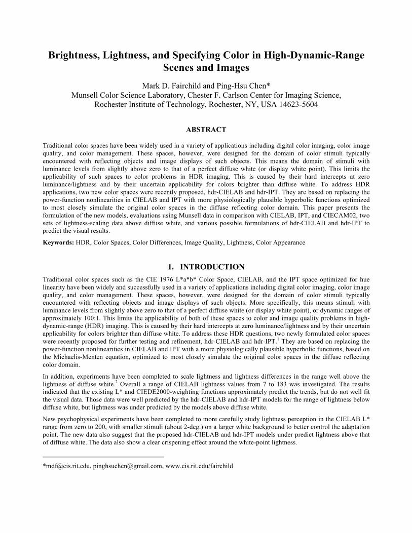
The same group of 17 color-normal observers participated in the SL2<100 and SL2>100 experiments, where 15 of them were also observers in the SL1 experiment. The total range of evaluated lightness values is from 0 to 200 at an interval of 12.5. The mean visual data are listed in the Table 1, together with the data of SL1.

Table 1. Two sets of mean experimental data on scaling lightness above diffuse white.

3. DERIVATION AND FORMULATION OF hdr-CIELAB AND hdr-IPT 3.1 hdr-CIELAB

Fairchild and Wyble1 proposed a basic structure for hdr-CIELAB to replace CIELAB L* by the Michaelis-Menten equation with the constraints of maximum perception, semi-saturation level, and offset. The equation is shown in Equation (1), and its optimized exponent was 1.50.

�

f (ω) =100 ωε

ωε + 0.184ε+ 0.02 (1)

To improve this equation, the first step was to find the semi-saturation point. The reason to apply the hyperbolic Michaelis-Menten equation to describe the lightness perception is that the visual perception is significantly nonlinear in part of stimulus range in log-log coordinates. It requires not only a power function to describe the relative linear range but also another function to describe the nonlinear decay from the power function4 and an offset to model threshold behavior. To find the turning point from the linear range to the nonlinear decay, the SL2 visual data were plotted in a log-log coordinate, as shown in Figure 5. In the figure, the solid line indicates the linear range. It was decided by analyzed the R2 values of the fitted lines for the visual data, as shown in Table 2. The R2 value of the normal diffuse reflecting range was 0.99, and changed from 0.99 to 0.98 between relative luminance of 1.78 and 2.57. According to this information, the semi-saturation was chosen as 2.

Evaluated SL1 Evaluated SL2Lightness X10 Y10 Z10 Lightness X Y Z180 3262.32 3691.53 4025.74 200 6931.18 7431.76 6177.06170 2268.98 2589.13 2816.54 187.5 4317.06 4601.18 3962.35160 1992.23 2277.76 2479.07 175 3454.12 3685.29 3122.35150 1693.03 1940.71 2121.46 162.5 2932.35 3124.71 2621.76140 1529.33 1756.29 1922.14 150 2403.53 2563.53 2164.06130 1343.59 1546.16 1690.64 137.5 1670.76 1774.71 1511.41120 1128.18 1303.05 1425.19 125 1408.76 1489.53 1274.94110 932.05 1075.76 1172.24 112.5 1075.82 1132.71 973.76100 729.78 842.01 903.26 100 968.08 996.98 883.5195 642.65 740.84 800.77 87.5 831.50 855.55 760.1190 547.58 630.78 678.14 75 635.43 653.62 580.8585 472.25 544.14 575.44 62.5 440.19 452.21 405.9080 375.98 432.96 453.40 50 296.81 304.64 278.3075 282.56 325.01 335.55 37.5 202.42 207.41 191.8170 221.04 253.95 259.19 25 125.27 127.82 117.4565 177.20 203.25 205.45 12.5 59.13 59.82 54.4760 136.55 156.39 157.41 0 0 0 0

Figure 5. The experimental setup of SL2>100

Table 2. The R2 value of fitted line for visual data ranged from the darkest one to itself.

The second improvement for deriving the equation was to set the maximum perception without constraint and decide it by optimization. There are seldom psychophysical experiments to derive the maximum lightness perception, and it is hard to assign a meaningful maximum perception.

For the constraint of the noise term in the equation, an offset of 0.02 was specified under the assumption that about 2% of diffuse white represents a reasonable level of visual noise for complex stimuli. These settings leave the exponent and maximum perception in the Michaelis-Menten equation to be optimized. It was optimized to minimize the difference between the Michaelis-Menten formulation and CIELAB L* for the L* range from 0 to 100 in relative luminance steps of 0.01, in order to most closely simulate the original color space in the diffuse reflecting color domain. The resulting exponent, ε, and maximum perception were 0.58 and 247, respectively. The RMS error in L* for the fit was 0.46. Figure 6 illustrates the L* function and fitted Michaelis-Menten function, Equation (2), as a function of relative luminance from 0 to 4.

�

f (ω) = 247 ωε

ωε + 2ε+ 0.02 (2)

Y/Yn L Log10(Y/Yn) Log10(L) R2

0.06 12.50 -1.22 1.10 -0.13 25.00 -0.89 1.40 -0.21 37.50 -0.68 1.57 -0.31 50.00 -0.51 1.70 -0.45 62.50 -0.34 1.80 -0.66 75.00 -0.18 1.88 -0.86 87.50 -0.07 1.94 -1.00 100.00 0.00 2.00 0.991.14 112.50 0.06 2.05 0.991.49 125.00 0.17 2.10 0.991.78 137.50 0.25 2.14 0.992.57 150.00 0.41 2.18 0.983.13 162.50 0.50 2.21 0.983.70 175.00 0.57 2.24 0.984.50 187.50 0.65 2.27 0.977.45 200.00 0.87 2.30 0.96

Figure 6. CIELAB L* and fitted Michaelis-Menten functions of relative luminance in the range from 0-4.

For imaging applications it is sometimes necessary to adjust the compressive nonlinearity to account for changes in surround relative luminance (Bartleson-Breneman) or absolute luminance level (Stevens Effect).5 This can be accomplished by modifying the exponent in the Michaelis-Menten function, ε, using factors to account for surround, sf, and luminance level, lf, as shown in Equations (3)~(5). Ys is the relative luminance of the surround and Yabs is the absolute luminance of the scene diffuse white in cd/m2. These are suggested surround and background adjustment factors that certainly require further study and optimization to various viewing conditions.

ε = 0.58 / (sf • lf ) (3)

�

sf = 1.25 − 0.25(Ys /0.184); (0 ≤Ys ≤1.0) (4)

�

lf = log(318) /log(Yabs) (5)

The formulation of the full hdr-CIELAB space is then given by Equations (6)~(10) by simply replacing the CIELAB cube-root-based function with Equation (2) and adjusting the normalization of the chroma dimensions by a factor of 1/100 to account for the scaling in Equation (2).

�

Lhdr = f (Y /Yn ) (6)

�

ahdr = 5[ f (X /Xn ) − f (Y /Yn )] (7)

�

bhdr = 2[ f (Y /Yn ) − f (Z /Zn )] (8)

�

chdr = ahdr2 + bhdr

2 (9)

�

hhdr = tan−1(bhdr /ahdr) (10)

3.2 hdr-IPT

The derivation of hdr-IPT followed the same constraints and procedure. The exponent in the Michaelis-Menten equation was optimized to minimize the difference between the Michaelis-Menten formulation and IPT I dimension for the I range from 0 to 1 in relative luminance steps of 0.01, to closely simulate the original color space. The resulting exponent, ε, and maximum perception were 0.59 and 246, respectively. The RMS error in I for the fit was 1.16. Figure 7 illustrates the I function and fitted Michaelis-Menten function, Equation (11), as a function of relative luminance from 0 to 4.

�

f (ω) = 246 ωε

ωε + 2ε+ 0.02 (11)

Figure 7. IPT I and fitted Michealis-Menten functions of relative luminance in the range from 0-4.

The exponent in the Michealis-Menten function, ε, is again modified using factors to account for surround, sf, and luminance level, lf, as shown in Equations (12)~(14).

ε = 0.59 / (sf • lf ) (12)

�

sf = 1.25 − 0.25(Ys /0.184); (0 ≤Ys ≤1.0) (13)

�

lf = log(318) /log(Yabs) (14)

The formulation of the full hdr-IPT space is then given by Equations (15)~(21) by simply replacing the IPT 0.43 power function with Equation (11).

�

LMS

⎡

⎣

⎢ ⎢ ⎢

⎤

⎦

⎥ ⎥ ⎥

= 0.4002 0.7075 − 0.0807−0.2280 1.1500 0.0612 0.0 0.0 0.9184

⎡

⎣

⎢ ⎢ ⎢

⎤

⎦

⎥ ⎥ ⎥

XD65

YD65

ZD65

⎡

⎣

⎢ ⎢ ⎢

⎤

⎦

⎥ ⎥ ⎥ (15)

�

′ L = f (L); L ≥ 0′ L = − f (−L); L < 0

(16)

�

′ M = f (M); M ≥ 0′ M = − f (−M); M < 0

(17)

�

′ S = f (S); S ≥ 0′ S = − f (−S); S < 0

(18)

�

Ihdr

Phdr

Thdr

⎡

⎣

⎢ ⎢ ⎢

⎤

⎦

⎥ ⎥ ⎥

=0.4000 0.4000 0.20000.4550 − 4.8510 0.39600.8056 0.3572 −1.1628

⎡

⎣

⎢ ⎢ ⎢

⎤

⎦

⎥ ⎥ ⎥

′ L ′ M ′ S

⎡

⎣

⎢ ⎢ ⎢

⎤

⎦

⎥ ⎥ ⎥

(19)

�

chdr−IPT = Phdr2 + Thdr

2 (20)

�

hhdr−IPT = tan−1(Thdr /Phdr ) (21)

4. APPEARANCE PREDICTIONS OF MUNSELL COLORS Wyble and Fairchild6 published an analysis of various color appearance models using the Munsell Renotation data.7 That analysis included the CIELAB, IPT and CIECAM97s models and used only those samples found in the gamut of the 1929 Munsell Book of Color. In the current analysis, similar computations were completed and visualized below. However, this analysis used the full set of 2734 real Munsell data points to provide a wider color gamut and included CIECAM02 and the two new spaces derived in this paper in addition to CIELAB and IPT. Moreover, CAT02 was used as the chromatic adaptation model for IPT and hdr-IPT models. It is expected that the performances of hdr- spaces will not be significantly different from their ldr- spaces models in the normal diffuse reflecting range, because their RMS errors for the fit were quite low. These new analyses represent the same hdr-IPT and hdr-CIELAB models as previously published with newly formulated hyperbolic nonlinearities.

4.1 Lightness

Figure 8 shows the lightness predictors of the five models as a function of Munsell Value. Perfect prediction of Munsell Value would be represented by a straight line with unity slope as seen for the CIELAB model and very closely for the IPT model. CIECAM02 shows a slight nonlinearity of prediction. The two revised HDR spaces do not exhibit significant difference comparing to their LDR spaces.

Figure 8. Model lightness predictors as a function of Munsell Value.

4.2 Chroma

Figure 9 shows the chroma predictors of the five models as a function of Munsell Chroma. Data points are color coded to their Munsell designations. Perfect prediction of Munsell Value would be represented by a straight line with unity slope and no scatter. One can see the well-known expansion of yellow chroma in CIELAB in comparison with the blue hues, as seen for the CIELAB model and very closely for the IPT model. CIECAM02 shows a slight nonlinearity of prediction. Again, the two new HDR spaces do not exhibit significant difference comparing to their LDR spaces.

Figure 9. Model chroma predictors as a function of Munsell Chroma.

4.3 Hue Linearity

Figure 10 shows the five model hue predictors as a function of Munsell Hue, again color coded by Munsell designation. Ideal results would be a perfect straight line. The well-known kink in the blue region of CIELAB is evident along with the relatively good behavior of IPT. The HDR versions of CIELAB and IPT show similar behavior to their LDR versions with respect to hue linearity.

Figure 10. Model chroma predictors as a function of Munsell Chroma.

An alternative analysis of hue linearity is visualized in Figure 11. In this case principal components analysis was performed on each hue slice (projected to the two chromatic dimensions) to determine the percent of variation explained by a single characteristic vector. A value of 100% would imply perfect hue linearity. Figure 11 encodes the percent of variation that is not described by the first characteristic vector (i.e., the amount of variation requiring a second dimension, or curve, to describe). Each model is represented by a row in the figure with the various hues represented by columns. Dark areas represent poor hue linearity with values represented by black meaning greater than about 7.5% variance is not described by one dimension. Mid-gray areas represent about 2.2% residual variation and white areas represent nearly perfect hue linearity. The rightmost column represents the average values ([IPT, hdr-IPT, CIECAM02, CIELAB, hdr-CIELAB] = [.734 .712 .707 .672 .681]) (average of first eigenvalue=[.988 .989 .986 .984 .985]). According to the average values, IPT shows its characteristic good hue linearity and hdr-IPT is similar and almost identical on average. CIECAM02, CIELAB, and hdr-CIELAB illustrate similar performance slightly worse than IPT.

Figure 11. Visualization of PCA analysis on the dimensionality of constant hue lines. Dark entries indicate that a significant amount of variation requires two dimensions to describe (an indication of hue nonlinearity). (The first and last rows are the representative colors of the hue angles form 0° to 351° at an interval of 9°.)

4.4 Hue Spacing

Hue spacing was evaluated by examining the hue angle distance between each neighboring Munsell Hue in each color space. Since there are 40 hue samples in the Munsell Renotation, each should be separated by 9 degrees in hue angle for uniform hue spacing. (Note it is possible to have good spacing with poor linearity and vice versa.) T-tests were performed to test the hypothesis that the average distance between adjacent hue planes is 9 degrees. A p>0.05 indicates that they hypothesis cannot be rejected. The visualization in Figure 12 renders the p values for each hue and the average in the last column. P values of near zero are shown as black and indicate poor hue spacing. P values rendered in white are near 1.0 with the mid gray representing p = 0.5. Each space shows significant deviation from equal hue spacing with IPT and hdr-IPT slightly worse than the others on average.

Figure 12. Results of t-tests on hue spacing. If each Munsell hue was equally spaced from its neighbors for a given model, the row of squares would be white. Black areas indicate hues with poor spacing.

5. WIDE-RANGE LIGHTNESS PREDICTIONS Both sets of visual data on wide-range lightness scaling, SL1 and SL2, were used to evaluate the hdr-CIELAB and hdr-IPT lightness scale, as shown in Figure 13 for the extended range and Figure 14 for the normal range. All models were normalized to predict a lightness of 100 for a relative luminance of 1.0. The SL2 visual data were used to derive the semi-saturation point, rather than to optimize the function. As a result, the data are still available for evaluation. For the range below diffuse white, each scale shows significant deviation from both sets of visual data. The differences of viewing conditions may cause the discrepancies. For the range above diffuse white, both hdr-CIELAB and hdr-IPT lightness functions under predict the perception, but some ranges are inside the error bar of SL2 visual data.

IPT hdr-IPT

CIECAM02 CIELAB

hdr-CIELAB

IPT hdr-IPT

CIECAM02 CIELAB

hdr-CIELAB

Figure 13. Prediction of lightness scaling data in a wide lightness range. Visual data are shown with their error bars for 95% confidence limit.

Figure 14. Prediction of lightness scaling data in the range from L*=0 to L*=100.

IPT and CIELAB lightness functions have better performance of prediction for the extended range. To improve the hdr-CIELAB and hdr-IPT lightness functions to fit the visual data, a power function for the noise term can be used to replace the fixed 0.02 offset. A sample formulation is shown in Equation (22). It leaves the maximum perception, exponent, and power function noise in the equation to be optimized. It can be optimized to minimize the difference between the formulation and CIELAB L* for an extended L* range, such as from 0 to 200 in relative luminance steps of 0.01 for normal range and 0.1 for extended range. Equation (23) is the resulting formulation for hdr-CIELAB. The RMS errors in L* for the fit were 1.26 for normal range and 1.31 for whole range. Equation (24) is the resulting formulation for hdr-IPT with the same procedure. The RMS errors in I for the fit were 2.72 for normal range and 2.65 for whole range. Figure 15 illustrates the lightness functions and the power functions of noise as a function of relative luminance from 0 to 6.5. The figure also shows the predictions of the visual data.

�

f (ω) = α ωε

ωε + 2ε+ βωβ (22)

�

f (ω) = 253 ω 0.61

ω 0.61 + 20.61+ ω1.88 (23)

�

f (ω) = 261 ω 0.65

ω 0.65 + 20.65+ ω 2.09 (24)

Figure 15. Prediction of lightness scaling data in a wide lightness range. The hdr- scales are improved from proposed models with a power function for the noise term.

The power function of the noise term is essentially to improve the performance of the Michaelis-Menten equation in the range of high physical stimuli, without a significant influence on the linear range of the lightness perception. It helps to describe the nonlinear decay of lightness perception together with the Michaelis-Menten equation. Moreover, instead of a constant, the ascending function of noise term may better describe the visual noise of human vision system, where the noise will be higher as the stimulus becomes higher.

Since these visual data are just two experiments on scaling wide-range lightness, it is premature to adjust either hdr- model to specifically fit these data by the power function for the noise term. Moreover, the maximum perception is not converged at certain level when applying the power function for noise, which should not be true that the maximum perception could be infinity. A noise function inversed before the saturation point is more reasonable. Furthermore, the adaptation in wide-range lightness scaling might need to be better understood. Given all of the above, it is likely that a different functional form of sigmoidal response function will be required to produce all the desired properties for an hdr- color space. Determination of the ideal function remains as future work.

6. CONCLUSIONS Two new color spaces, hdr-CIELAB and hdr-IPT, were modiefied to allow extension of the CIELAB and IPT color spaces for use in HDR imaging applications. Their overall performance in predicting Munsell Renotation appearances is similar to the traditional versions of these spaces. These spaces provide interesting combinations of colorimetric fidelity and physiological plausibility and pose interesting new questions for developers of color spaces and imaging systems. At this point, these spaces should be considered proposals as there is certainly a need for more testing, collection of more HDR visual data, and refinement of the models. They do, however, show promise for future applications in color specification, device characterization, image difference metrics and image quality evaluation.

REFERENCES

[1] M.D. Fairchild and D.R. Wyble, hdr-CIELAB and hdr-IPT: Simple Models for Describing the Color of High-Dynamic-Range and Wide-Color-Gamut Images, IS&T/SID 18th Color Imaging Conference, San Antonio, 322-326 (2010).

[2] P. Chen, M.D. Fairchild, and R.S. Berns, Scaling Lightness Perception and Differences Above and Below Diffuse White, IS&T/SID 18th Color Imaging Conference, San Antonio, 42-48 (2010).

[3] A.E.O. Munsell, L.L. Sloan, and I.H. Godlove, Neutral value scales, I, Munsell neutral value scale, Journal of the Optical Society of America 23, 394-402 (1933).

[4] C.J. Bartleson and E.J. Breneman, Brightness perception in the complex fields, Journal of the Optical Society of America 57, 953-956 (1967).

[5] M.D. Fairchild, Color Appearance Models, Second Edition, Wiley-IS&T Series in Imaging Science and Technology, Chichester, UK (2005).

[6] D.R. Wyble and M.D. Fairchild, Prediction of Munsell appearance scales using various color appearance models, Color Research and Application 25, 132-144 (2000)

[7] S.M. Newhall, Preliminary report of the O.S.A. subcommittee on the spacing of the Munsell colors, Journal of the Optical Society of America 30, 617-645 (1940).