SLAC - 331 -UC-28

(4

EGUN-AN ELECTRON OPTICS AND GUN DESIGN PROGRAM

W. B. Herrmannsfeldt

Stanford Linear Accelerator Center

Stanford University

Stanford, California 94309

October 1988

Prepared for the Department of Energy

under contract number DE-AC03-76SF00515

Printed in the United States of America. Available from the National Techni- cal Information Service, U.S. Department of Commerce, 5285 Port Royal Road, Springfield, Virginia 22161. Price: Printed Copy A07, Microfiche AOl.

ABSTRACtI? - -

The name EGUN has become commonly associated with the program also

known as the SLAC Electron Trajectory Program. This document is an updated

version of SLAC-226,’ published in 1979. The program itself has had substantial

upgrading since then, but only a few new features are of much concern to the

user. Most of the improvements are internal and are intended to improve speed

or accuracy.

EGUN is designed to compute trajectories of charged particles in electrostatic

and magnetostatic fields, including the effects of space charge and self-magnetic

fields. Starting options include Child’s Law conditions on cathodes of various

shapes, as well as user specified initial conditions. Either rectangular or cylindri-

cal symmetry may be used. In the new jargon, the program is a 2-l/2 dimension

code meaning 2-D in all fields and 3-D in all particle motion. A Poisson’s Equa-

tion Solver is used to find the electrostatic fields by using difference equations

derived from the boundary conditions. Magnetic fields are to be specified exter-

nally by the user, by using one of several methods including data from another

program or arbitrary configurations of coils.

This edition of the documentation also covers the program EGN87c, which is

a recently developed version of EGUN designed to be used on the newer models

of personal computers, small main frames, work stations, etc. The EGN87c

program uses the programming language C which is very transportable so the

program should operate on any system that supports C. Plotting routines for

most common PC monitors are included, and the capability to make hard copy

plots on dot-matrix printer-plotters is provided.

TABLE OF CONTENTS ~-- -

1 Introduction ............................ 1 2 Application ............................ 2

3 Poisson Equation Solver ...................... 9

3.1 General Description ................... 9

3.2 Problem Input ...................... 11

Title and Potential Cards ................ 15 POTN, Rect. or Cyl. Coordinates ............ 16

Magnetic Field Data ................... 19

Boundary Input ..................... 20

Special Boundary Conditions ............... 28

Grids ........................... 28 Boundary Diagnostics .................. 30

3.3 Poisson’s Equation Solver ................ 32

4 Starting Conditions ........................ 35

4.1 Universal Parameters .................. 36 PERVO .......................... 36 HOLD Emission limited ................. 37 PE ............................ 38 ERROR .......................... 38 UNIT, UNITIN ...................... 39

LSTRH .......................... 39 MAXRAY ........................ 39 STEP ........................... 39 NS ............................ 40 SPC ............................ 41 PHILIM ......................... 42 SAVE=l, Boundaries ................... 42

SAVE=2, Trajectories .................. 44

MASS ........................... 45 AV and AVR ....................... 45 BEND .......................... 46 MAGMLT ........................ 47 IPBP ........................... 47 ZEND ........................... 47 VION ........................... 48 ZDOTEQ, EBQ Mode .................. 48

4.2 Equipotential P1ol.s ................... 49

EQUIPR ......................... 50

LM .................. . ......... 50 EQLN.. ......................... 50

EQST ........................... 50

IZl,IZ2andIZS ..................... 51

4.3 Plotting Controls .................... 51

SCAL%=‘YES’ ...................... 51 SXandSY ........................ 51

4.4 Magnetic Fields ..................... 52

Magnetic Field Input ....................... 53

Axial Magnetic Field ................... 53

MAGORD, Order and Direction ............. 56

NMAG Ideal Coils .................... 57 Off-Axis Expansions. I ...... ; ........... 58

Rect. Coord. Expansions ................. 59

Elliptic Integrals ..................... GO

Vector Potential Data .................. 61 4.5 General Cathode and GENCAR.D ............ G2 4.6 Spherical Cathode .................... 70

4.7 Card Starting ...................... 74

User Specified Data .................... 76

Prograxn Generated Cards ................ 78

Thermal Effects ...................... 79 Rectangular Coordinates with Cylindrical Beams .... 79

4.8 Laplace’s Equation Applications ............. 82

4.9 Dielectric Boundaries .................. 83 5 Trajectory Calculations ...................... 87

6 Trajectory Analyses ........................ 91

References .............................. 04 Appendix I, Equation:; of Motion .................. 96

Apperldix II, General Neumann l3ounclary ............ 104

Appendix III, Condensed Inst.rllctions ............... 107

Appendix IV, Boundary Examples ................ 120

1 -

TABLE OF FIGURES ~-- - -

1 Simulation of a Pierce Diode ................... 7

2 Section of mesh for solution of Poisson’s Equation ........ 9

3 Example of preparation to run a problem ............. 13

4 Fortran data prepared for the problem shown in Fig. 3 ...... 14

5 Program output from the boundary data shown in Fig. 4 .... 25

6 Basic geometry for spherical cathode configurations ....... 72

7 Plotted output of sample problem shown in Fig. 3 ........ 73

A-II General Neumann Boundaries ................ 104

A-IV Boundary Example Figures ................. 120

--

1. INTRODUCTION ~~. - -

This report is intended as a user’s reference manual for the EGUN Electron

Trajectory Program. It contains all the currently relevant material from the

earlier publications about this program which were SLAC-51 and SLAC-166 and

SLAC-226.l In addition, it includes specific instructions for using a number of

the special features which have been added to the program. These features

have usually been incorporated as a direct result of the needs of some particular

user and we wish to take this opportunity to express thanks to everyone who

has at some time or other suggested improvements to the program. We have

all benefited by this open process and it is for the purpose of making all these

features better available that this report is being prepared.

This edition of the documentation also covers a recently developed version

of the program called EGN, written in C2 and designed to be used on the newer

models of Personal Computers. Plotting routines for most common PC monitors

are included, and the capability to make hard copy plots on dot-matrix printer-

plotters is provided. The plotting routines provided are based on a commercial

package called Metawindow(R) by Metagraphics.3 Metawindow supports most

common hardware configurations. All of the physics options and input data are

the same for the two versions except that EGN uses free field input for boundary

and trajectory data. Both programs use essentially the same NAMELIST files.

Computer implementation of EGN is covered in a separate note prepared espe-

cially for the appropriate hardware. Prospective users of EGN can check with

the author to find what hardware is supported, but it is likely that EGN would

operate on any system for which a C compiler is available. In the present PC

version, the code requires around 400 kbytes of storage. It operates about 30-60

1

times slower on a PC than it does on the IBM-3080 series mainframe. A typical

space-charge limited Pierce diode may need 20 seconds on the 3081 and lo-20

minutes on a PC, depending on the hardware configuration.

2. APPLICATION

The SLAC Electron Optics Program is specifically written to calculate elec-

tron trajectories in electrostatic and magnetostatic fields. Poisson’s equation is

solved by finite difference equations using boundary conditions defined by spec-

ifying the type and position of the boundary. Electric fields are determined by

differentiating the potential distribution. The electron trajectory equations are

fully relativistic and account for all possible electric and magnetic field compo-

nents. Space charge forces are realized through appropriate deposition of charge

on one cycle followed by another solution of Poisson’s equation which is in turn

followed by another cycle of trajectory calculations.

The program may be used in either rectangular or cylindrical coordinates. A

special option allows space charge forces for a cylindrical beam to be calculated in

a rectangularly symmetric array of electric and magnetic fields. Magnetic fields

are read in either as axial strengths or as arrays of coils with specified coordinates

and currents. The preferred technique of defining the magnetic field is to calculate

the axial field from an arbitrary configuration of solenoids. Alternatively, the

program accepts the output data from a magnet design program, which can

include the effects of saturable iron. In cylindrical coordinates, the magnetic

fields are axially symmetric. Off-axis field components are calculated by a sixth-

order expansion of the radial coordinate.

Electron trajectories may be started by one of four schemes:

2

-- -

times slower on a PC than it does on the IBM-3080 series mainframe. A typical

space-charge limited Pierce diode may need 20 seconds on the 3081 and 10-20

minutes on a PC, depending on the hardware configuration.

2. APPLICATION

The SLAC Electron Optics Program is specifically written to calculate elec-

tron trajectories in electrostatic and magnetostatic fields. Poisson’s equation is

solved by finite difference equations using boundary conditions defined by spec-

ifying the type and position of the boundary. Electric fields are determined by

differentiating the potential distribution. The electron trajectory equations are

fully relativistic and account for all possible electric and magnetic field compo-

nents. Space charge forces are realized through appropriate deposition of charge

on one cycle followed by another solution of Poisson’s equation which is in turn

followed by another cycle of trajectory calculations.

The program may be used in either rectangular or cylindrical coordinates. A

special option allows space charge forces for a cylindrical beam to be calculated in

a rectangularly symmetric array of electric and magnetic fields. Magnetic fields

are read in either as axial strengths or as arrays of coils with specified coordinates

and currents. The preferred technique of defining the magnetic field is to calculate

the axial field from an arbitrary configuration of solenoids. Alternatively, the

program accepts the output data from a magnet design program, which can

include the effects of saturable iron. In cylindrical coordinates, the magnetic

fields are axially symmetric. Off-axis field components are calculated by a sixth-

order expansion of the radial coordinate.

Electron trajectories may be started by one of four schemes:

‘2

1. “GENERAL” cathode in which electrons are started assuming Child’s law

holds near a surface designated as the cathode.

2. “SPHERE” for a spherical cathode (cylindrical in rectangular coordinates)

in which the electrons are assumed to be emitted at right angles to the

surface defined by a radius of curvature and a radial limit. Child’s law for

space charge limited current is again used.

3. “CARDS’ in which the specific starting conditions for each ray are specified

in an 80-column card format.

4. “GENCARD” which combines the versatility of “CARDS” with the calcu-

lation of emission using Child’s law as in “GENERAL.”

On the first iteration cycle, space charge forces are calculated from the as-

sumption of paraxial flow. As the rays are traced through the program, space

charge is computed and stored in a separate array. After all the electron tra-

jectories have been calculated, the program begins the second cycle by solving

Poisson’s equation with the space charge from the first cycle. For problems meet-

ing the paraxial assumptions, especially if relativistic electron beams are involved,

this one cycle may be sufficient to solve the entire problem. For other problems

in which space charge is negligible, e.g., spectrometers and phototubes, a single

cycle is usually adequate.

Subsequent iteration cycles (as many as are requested) follow the above pat-

tern. The Child’s law calculations for the starting conditions are remade by

averaging the perveance used for the previous cycle with the perveance calcu-

lated directly from the solution of Poisson’s equation.

An additional starting option is “LAPLACE” intended for any application of

Laplace’s equation not involving electron ray tracing. In this case the number of

3

-- -

cycles is used simply to improve the accuracy of the solution of Laplace’s equation.

The “LAPLACE” option includes a provision for inputting arbitrary data in the

“space charge” array. The output from LAPLACE includes a list of the fields on

the entire boundary. This can be used to find local peak field strengths and to

calculate the electrical capacity of part or all of some configuration.

The Poisson Solver program always operates in two dimensions; either R

and Z in cylindrical coordinates or Y and X in rectangular coordinates. The

rectangular coordinate output retains the R and Z labels. Electron orbits are

calculated through azimuthal angles, (labeled “PHI”) referenced to the Z axis.

In rectangular coordinates, PHI is actually the third Cartesian coordinate.

Magnetic fields, except for the self-magnetic field of a beam, are input directly

in one of three ways:

1. by specifying the field along the Z-axis, (two methods are provided)

2. by specifying a set of point coils (giving position, radius and current), or

3. by using the vector potential output from a magnet program such as Pois-

son. It is interesting to note that Colman4 has converted several accelerator

physics programs including Poisson to run on the IBM-AT.

In cylindrical coordinates, the magnetic field is interpreted as an axial field

with radial terms as required by Maxwell’s equations. The off-axis fields can be

made by either a sixth order expansion from the axial fields or, for the case of a

set of coils, by directly using the appropriate elliptic functions. Second or fourth

order expansions can be selected if the quality of the data cannot support the

sixth order expansions. When the vector potential input has been used, local

interpolation is used in place of the expansion.

4

In rectangular coordinates the magnetic field -can be -defined to be principally

in any one of the three Cartesian directions. Off-median-plane fields are found

by expansion of the coordinate in the direction normal to the median plane. If

the median plane is the R-Z plane, then the field is in the PHI direction and

the field extends to infinity in the R-direction. This fits the configuration of the

pole face of a dipole magnet. (Remember that R, Z and PHI are here taken to

be orthogonal Cartesian coordinates.) If the median plane lies normal to the

plane of the problem, through the Z-axis, then the field extends to infinity in the

PHI direction. In this case the direction of the field on the median plane can

be either in the Z-direction or in the R-direction, depending on the symmetry of

the coils that produce the field. The off-median-plane expansions in rectangular

coordinates satisfy Maxwell’s equations to second order.

Self-magnetic fields are calculated for both coordinate systems from the cur-

rent in the rays on the present cycle. A built-in sort routine insures that the

rays are sequentially numbered from the axis outwards. The self-magnetic field

calculation assumes all the current from the previous rays lies on the axis in an

infinitely long conductor. If the ray being calculated crosses the last preceding

ray, then the current from that ray is dropped. However, if the ray continues to

cross other rays, then the current from those rays is only dropped if the ray goes

below the minimum radius of a previous ray. If several rays cross, the results

are apt to be somewhat incorrect, depending of course, on how significant the

self-magnetic field is. Note that if the self-magnetic field is very significant, then

almost by definition, one is dealing with a very intense relativistic beam. This

problem is generally better suited to the paraxial ray approach, as solved in the

first cycle, in which the space charge is offset by the self-magnetic field directly,

5

rather than by the off-setting effects of two large terms. For cases where the

beam is already relativistic in the gun, a new option allows the user to define a

velocity above which the direct cancellation of space charge by the self magnetic

field is used instead of the normal separate terms. This permits the Child’s Law

calculation to be used near the cathode and the paraxial calculation to be used

when the beam is at higher energy. This velocity level is given in units of v/c

using the parameter ZDOTEQ.

In rectangular coordinates, the self-magnetic field assumes symmetry about

the Y = 0, (R = 0) plane. If this is not correct, or if for other reasons it is

desired to turn off the self-magnetic field, then an external field of strength zero

can be specified. In any case, in rectangular coordinates, the self-magnetic field

functions only if there is no external field in the PHI direction.

A single variable controls plotting. If this variable, MI is set to zero to reject

all plotting, then on the first and last cycles, every tenth point that would have

been plotted is printed so that it may be hand plotted. Normally at least the last

cycle is plotted. The first cycle may also be plotted or one may even plot every

cycle. All plots may include equipotential plots, either separate or overlaid with

the trajectory plots.

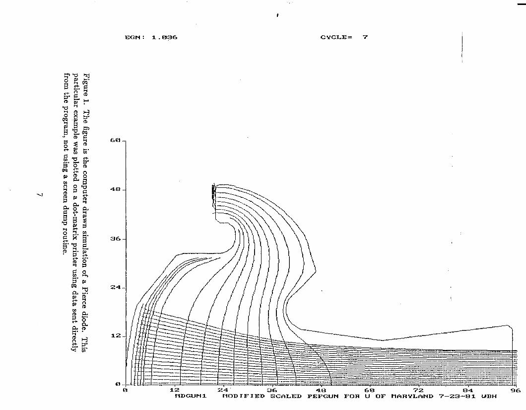
Figure 1 is an example of the graphic output showing a Pierce diode with

equipotential lines and trajectory paths. If there is an external magnetic field,

then this field is also plotted, overlaid on the trajectory plots. A special option

allows one to choose a single trajectory, IPHI for which the azimuthal position

PHI, is plotted as a function of Z.

6

P . 74

. .

Figure 1.

The figure

is the com

puter drawn

simulation

of a Pierce diode.

This particular

example

was plotted

on a dot-matrix

printer using

data sent

directly from

the

program,

not using

a screen dum

p routine.

7

There are a pair of diagnostic plots; current density vs. - radius and alpha

vs. radius. (Alpha = arctan dR/dZ). Th ese are plotted using the final data of

the last cycle, so that the radius plotted is the final R coordinate. The current

density plot is constructed by creating ten bins in the space between R=O and

the largest R value, and plotting the current that falls in each bin; the result can

be rather ragged even for a fairly uniform beam, unless many trajectories are

used.

A diagnostic routine is called at the end of the program to calculate the emit-

tance using the so-called edge emittance which is four times the rms emittance.

Both the actual emittance and the invariant or normalized emittance are calcu-

lated; the momentum of the first ray is used to define the beta-gamma product

that is used to determine the normalized emittance.

If the plotting parameter MI is defined as a negative number, the programs

interpret this as a deliberate fatal boundary error. The program will then plot

the boundary as well as provide all diagnostics of the boundary data. This is

a useful way to preview the boundary plot without spending time running the

entire program.

8

3. POISSON EQUATION SOLVER -

3.1 GENERAL DESCRIPTION

The program contains subroutines which read in data cards describing the

boundary conditions and calculate the coefficients of the finite difference equa-

tions for each mesh point within the problem. The subroutine POISSN is then

called to generate the solution to Poisson’s equation which match those bound-

ary conditions. The solution is found in terms of a set of points which form a

mesh of identical squares. It is recognized that a provision for a rectangular mesh

(i.e., different horizontal and vertical spacing) would improve the utility of the

program and it is planned to incorporate this feature as soon as possible. The

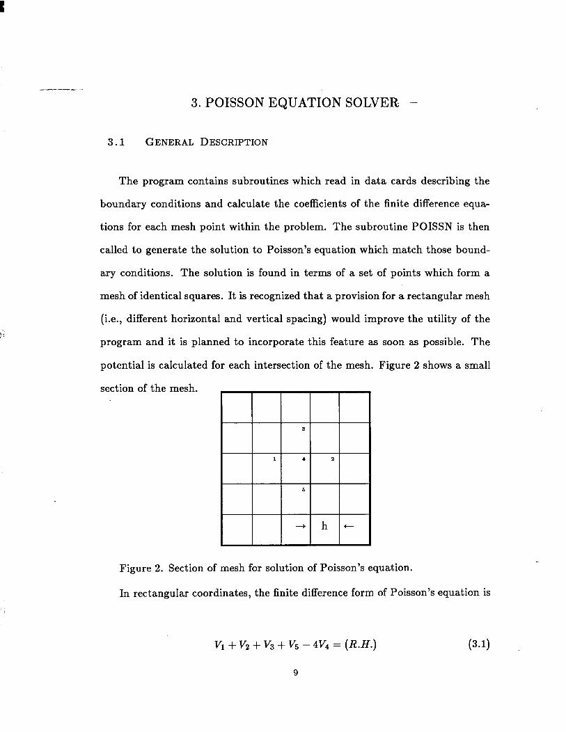
potential is calculated for each intersection of the mesh. Figure 2 shows a small

section of the mesh.

Figure 2. Section of mesh for solution of Poisson’s equation.

In rectangular coordinates, the finite difference form of Poisson’s equation is

vl + v2 + v3 + v5 - 4v4 = (R.H.)

9

(3.1)

where the V’s refer to the numbered points in Fig. 1 and.R.H.- is the value of the

right-hand side of Poisson’s equation at point 4 when written in the form

v2v = p/c2 (3.2)

All equations use the mesh space, h, as the basic unit, so h does not appear

explicitly.

For problems with cylindrical symmetry, the finite difference equation be-

comes

RVl + Rv2 -t (R-t i/z)& -t- (R - i/2)6, - 4Rv4 = R X (R.H.) P-3)

where R is the distance in mesh units from the axis of symmetry to the point at

4.

A number of references5-7 give the derivation of these difference equations

and of the special equations at boundaries. Three types of boundaries are of

interest. A Dirichlet boundary is that boundary on which the potential is known.

In an electrostatic problem, this would be an electrode fixed at a given potential.

An ordinary Neumann boundary is one which lies coincident with the mesh and

on which the normal derivative of the potential is known. In practice, the only

value of the normal derivative that is ever known is zero. Thus, for example, the

axis of symmetry of a cylindrically symmetric device has the normal derivative

equal to zero and is a Neumann boundary.

However, the axis of a cylindrical symmetry problem is a special case of which

the difference equation is

VI + V2 + 4V3 - 6V4 = (R.H.) (3.4

The difference equation for ordinary Neumann boundaries parallel to either axis

can be derived from Eqs. (3.1), (3.3) or (3.4) by setting the potentials which

10

straddle the boundary equal to each other. Thus a vertical Neumann boundary

in cylindrical coordinates has the form

2RVl,2 + (R + l/Z)& + (R - l/Z)&, - 4RV4 = R x (R.H.) P-5)

where the subscript 1 or 2 applies to the point inside the problem.

The third type of boundary is the general Neumann boundary, i.e., one which

does not lie along a mesh line. It is always assumed that the normal derivative

is zero. The program has a provision for overriding the internally computed

difference coefficients and it is feasible to hand calculate difference coefficients

for a general Neumann boundary. There is a derivation of these coefficients in

Appendix II. However, in practical applications to electron optics problems, it is

only rarely necessary to go to such extremes.

A special case of general Neumann boundary which can be handled easily is

the 45’ Neumann boundary. All that is required is to specify each successive point

using the ordinary Neumann condition for both coordinates; i.e., both DELTAR

and DELTAZ = 0. A tilted boundary that is sufficiently far from the area of

most interest can frequently be adequately approximated by a combination of

normal and 45’ Neumann boundaries.

3.2 PROBLEM INPUT

In this section the rules for problem input will be described using an actual

example and following through the process line by line. The new user is urged to

read this section carefully while the old user or reader trying to gain an overall

familiarity with the program may well skip this section. In this section especially,

no attempt will be made to be concise.

Condensed instructions for problem input are maintained with the source

listing and are intended to be up-to-date. A copy of the current version of these

11

instructions is printed in Appendix III. The reader should followthe instructions

which are relevant to this discussion while studying the example.

Except for the TITLE, boundary input, and ray starting cards, all input to

the program is by means of the NAMELIST option by which certain variables

are defined at the place in which the program expects them.

The definitions are by means of short defining statements, e.g., RLIM = 50.

A given set of these statements may be placed on one card, but the number of

data cards used is unimportant. Each set of inputs is preceded by a designator,

e.g., &INPUTl, which must begin in column 2. Never use column 1 of any

NAMELIST card. The NAMELIST block is closed by an &END entry. The

order of the entries is unimportant and not all parameters need to be included.

Reasonable default values have been assigned to all NAMELIST parameters,

especially for the rarely used ones for which the default value is usually designed

to cause the parameter to be ignored. Array elements can be defined with their

subscripts but it is usually preferable to give the name of the array followed by

a string of numbers separated by commas. All entries are spaced by commas; a

final comma before the &END is optional.

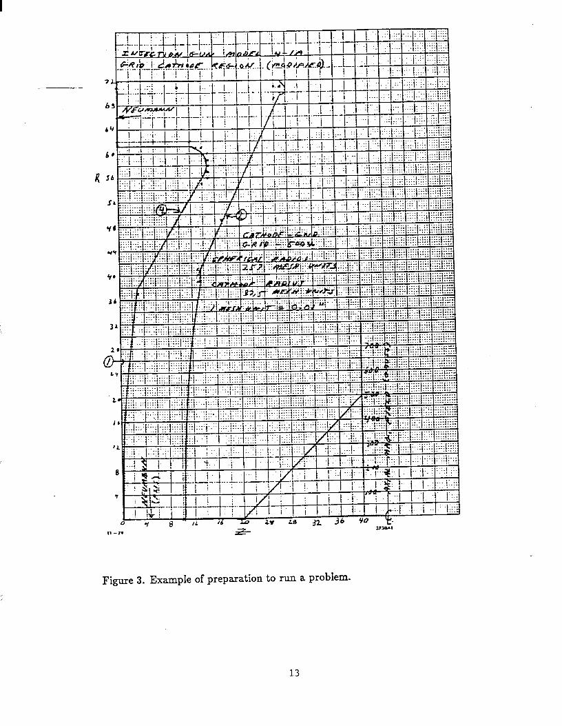
Preparation for running a problem consists of making a suitable scale drawing

on graph paper. Figure 3 shows the region between cathode and grid for the

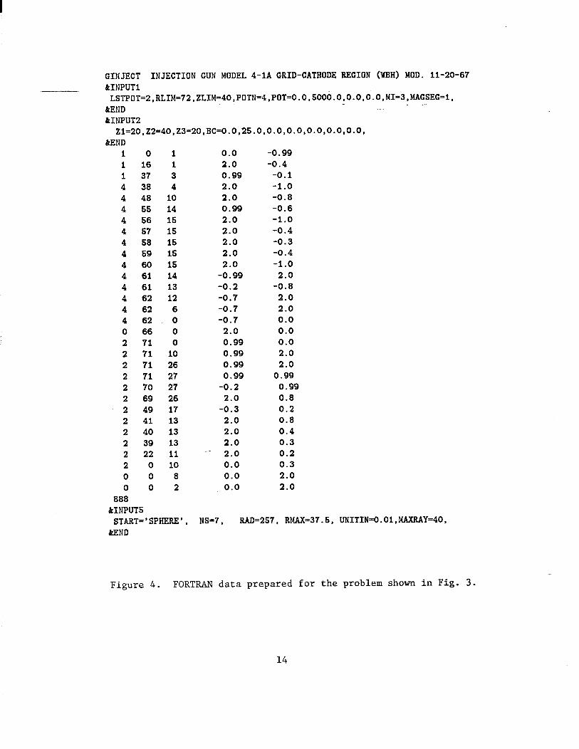
SLAC injection gun. Figure 4 is the line-by-line listing of the input data.

12

q::q ; +;:-} :I.:.:l. :.I ‘..I.+} 1

*, . f -&w- :y. ,yr l . , . j . . . . , . . . . , . .

Figure 3. Example of preparation to run a problem.

13

GINJECT INJECTION GUN MODEL 4-IA GRID-CATHODE REGION (WBH) MOD. 11-20-67 &INPUT1 --

LSTPOT=2,RLIM=72,ZLIM=40,POTN=4,POT=O.0,500~.0,0.0,0.0,MI=3,MAGSEG=l, _ - &END . &INPUT2

Z1=20,Z2=40,Z3=20,BC=0.0,25.0,0.0,0.0,0.0,0.0,0.0, &END

10 1 16 1 37 4 38 4 48 4 55 4 56 4 57 4 58 4 59 4 60 4 61 4 61 4 62 4 62 4 62 0 66 2 71 2 71 2 71 2 71 2 70 2 69 2 49 2 41 2 40 2 39 2 22 2 0 0 0 0 0

888 &INPUT5

1 0.0 -0.99 1 2.0 -0.4 3 0.99 -0.1 4 2.0 -1.0

IO 2.0 -0.8 14 0.99 -0.6 15 2.0 -1.0 15 2.0 -0.4 15 2.0 -0.3 15 2.0 -0.4 15 2.0 -1.0 14 -0.99 2.0 13 -0.2 -0.8 12 -0.7 2.0

6 -0.7 2.0 0 -0.7 0.0 0 2.0 0.0 0 0.99 0.0

10 0.99 2.0 26 0.99 2.0 27 0.99 0.99 27 -0.2 0.99 26 2.0 0.8 17 -0.3 0.2 13 2.0 0.8 13 2.0 0.4 13 2.0 0.3 11 -- 2.0 0.2 10 0.0 0.3

8 0.0 2.0 2 0.0 2.0

START='SPHERE', NS-7, RAD=257, RMAX=37.5, UNITIN=O.Ol,MAXRAY=40. &END

Figure 4. FORTRAN data prepared for the problem shown in Fig. 3.

14

--

Title and Potential Cards _ -

(TITLE) Th e fi t rs card of the data set is the title card. The contents of this

card will appear at various points in the printed output and as the title for the

plots. A line up to 80 characters long may be used with any alphanumeric string.

The second card is &INPUTl, starting in column 2.

The following remarks about array limits apply specifically to the current

version of the program. Refer to the condensed set of instructions for array

limits valid with the version that you have. It is suggested that most problems

should use about 5000 mesh points although there are occasions when much

smaller, or somewhat larger, numbers of mesh points are useful. It is virtually

always possible to break a problem up into sections that are not appreciably

larger than about 5000 to 8000 mesh points. Present versions of the programs

do not “charge” for points between the upper boundary of a problem and RLIM.

The third card is the potential card. It contains the basic information for

setting up the program. Actually, any number of lines or cards can be used to

specify the data.

( RLIM) RLIM is the maximum size of the problem area in the radial direc-

tion. RLIM is a positive integer; the present limit is 100.

(ZLIM) ZLIM is th e maximum size of the problem in the axial direction. A

larger than necessary value of ZLIM may affect the way the plots are scaled. If an

attempt is made to create a boundary which exceeds the limits RLIM by ZLIM,

or goes negative, error messages are printed and the program will not attempt

the solution of Poisson’s equation. ZLIM is a positive integer; the present limit is

300. The present limit for the total area is 11001 mesh points in the FORTRAN

program and 8001 in the C version.

(IAX) IAX p fi s eci es a depressed axis in cylindrical coordinates. It can be used

for a hollow beam device or for a device that is really in rectangular coordinates

but for which it is desired to use some cylindrical features, such as the elliptic

15

-- -

integral specification of the magnetic field. IAX is aninteger with the default

value IAX=O.

(POTN) POTN is the number of potentials which are to be read in. There

may be reasons to assign different numbers to parts of surfaces which are at the

same potential. Normally the cathode will be potential number 1 and the anode

will be number 2. Usually the grid, if any, will be number 3. A focus electrode,

even if at cathode potential, should be assigned a different number to enable

the general cathode starting method to be applied. If an electrode, such as a

thin grid support, can intercept a trajectory, the ray may pass right through the

electrode as if it was a thin ideal grid. If the focus electrode is given the potential

number 4, or 14, 24, etc., a trajectory will stop when within one mesh unit of

the electrode. These numbered electrodes also stop equipotential lines that get

close. Potential 5 is used for a hollow cathode or a shadow grid and should not

be used for the focus electrode. The present limit for POTN is 101.

POTN is a positive integer for cylindrical symmetry.

- POTN is a negative integer for rectangular symmetry.

RECTANGULAR COORDINATES. The code to the program to switch to

rectangular coordinates is the sign of POTN. If POTN is negative, the program

assumes rectangular symmetry and a message: ***RECTANGULAR COORDI-

NATES, PHI IS TRANSVERSE appears immediately after the list of potentials.

POT(I) The next numbers are the elements of the array of potentials. They

are read in order from 1 to POTN. Potentials are carried in double precision

which means that up to 15 significant decimal figures can be used. Examples

of valid ways of punching 250 volts are as follows: 250., 250, 2.5302, 2500E-

1, 250.000. For NAMELIST, the list need consist only of POT = (string of

potentials separated by commas).

POT(I) is an element of an array of floating point numbers.

Negative potentials are indicated by a minus sign, e.g., -250. Negative po-

16

tentials are permitted but it is preferable to avoid using-them. Since a constant

can always be added to all potentials, it is possible to make the most negative

potential zero. The reason for avoiding negative numbers is that space charge is

negative and some diagnostics of the output are simplified if there are no negative

potentials. On the other hand, certain problems have a symmetry that can be

quickly examined if a symmetry plane or surface is made to be zero by having

equal + and - potentials. Then negative potentials are certainly desirable.

Note that it is acceptable to include potentials corresponding to potential

numbers which are not used by the problem. One reason for doing this is to get

a desired set of equipotential lines on the plotter output.

The program is intended to be run using engineering units. Thus potentials

are in volts and magnetic fields are in gauss. If a problem does not use magnetic

fields or relativistic energies, there is no reason not to scale the potentials. The

perveance and running time will not be affected. However, there is also nothing

gained by scaling. Of course, when a problem has been run at one set of poten-

tials, all the scaling rules of electron optics may be applied to avoid the cost of

running the problem again.

(MI) MI is a code number which determines the selection of plots.

If MI = 0 there are no plots generated. However, every tenth point of the

trajectories is printed for the first and last cycles. Refer to the condensed in-

structions for a table showing the available options for MI.

MI is a positive integer or zero. If MI is negative it is interpreted as a

deliberate boundary error for help in debugging boundaries.

TYME is used to make an internal check of how much time is being used to

guard against running out of computer time, as specified on a JOB card, just

before printing and plotting the results. TYME uses special machine language

subroutines to measure actual use of CPU time which is the parameter used to

determine JOB time and charges in a multitask environment. This avoids gross

variations in time due to the presence of other jobs on the system. The subroutine

17

must be supplied by non-S-tanford users to suit their hardware or, alternatively,

dummy subroutines may be used to defeat this feature. The program only tests

for TYME once each cycle and determines that there is adequate time left to do

the extra plotting, etc., that is involved in the last cycle, based on the previous

cycle time.

When time appears limited, the program cuts out intermediate cycles, with a

note that: THERE IS NOT ENOUGH TIME TO DO THE SPECIFIED NUM-

BER OF CYCLES. TYME does not need to correspond exactly to the job card.

The user may wish to modify the value according to his experience, or disable

TYME entirely by setting it much larger than his JOB card time.

In a PC environment, TYME will cause the program to drop intermediate

cycles, with the above message, but will not cause the program to be terminated

early. However, users should be careful to allow enough time, or watch the screen

carefully to see that cycles are not skipped inadvertently.

LSTPOT = 1, 2 or 3 causes the program to print a table of the potentials of

all- the mesh points. This is the most useful diagnostic available for the Poisson

solution and, when studied together with the equipotential plot, can show quite

subtle errors. The default value; LSTPOT = 0, suppresses this output and thus

saves quite a lot of printing if the same or a very similar boundary is run many

times. The choices for LSTPOT cause the printing of the first (LAPLACE)

solution (LSTPOT = i), or the last solution (LSTPOT = 2), or the solutions

from both the first and last cycles (LSTPOT = 3).

The parameter MAGSEG controls two of the four possible ways of reading

in magnetic fields. The example case will be explained in the next section.

Three additional parameters have been added to the PC program to control

the solution of Poisson’s equation;

1. PASS is an integer controlling the number of passes made by the Poisson

solver for the initial solution. The default value is PASS=2, but for prob-

18

lems without space charge, it is sometimes- desired-to converge to a better

solution before doing any ray tracing.

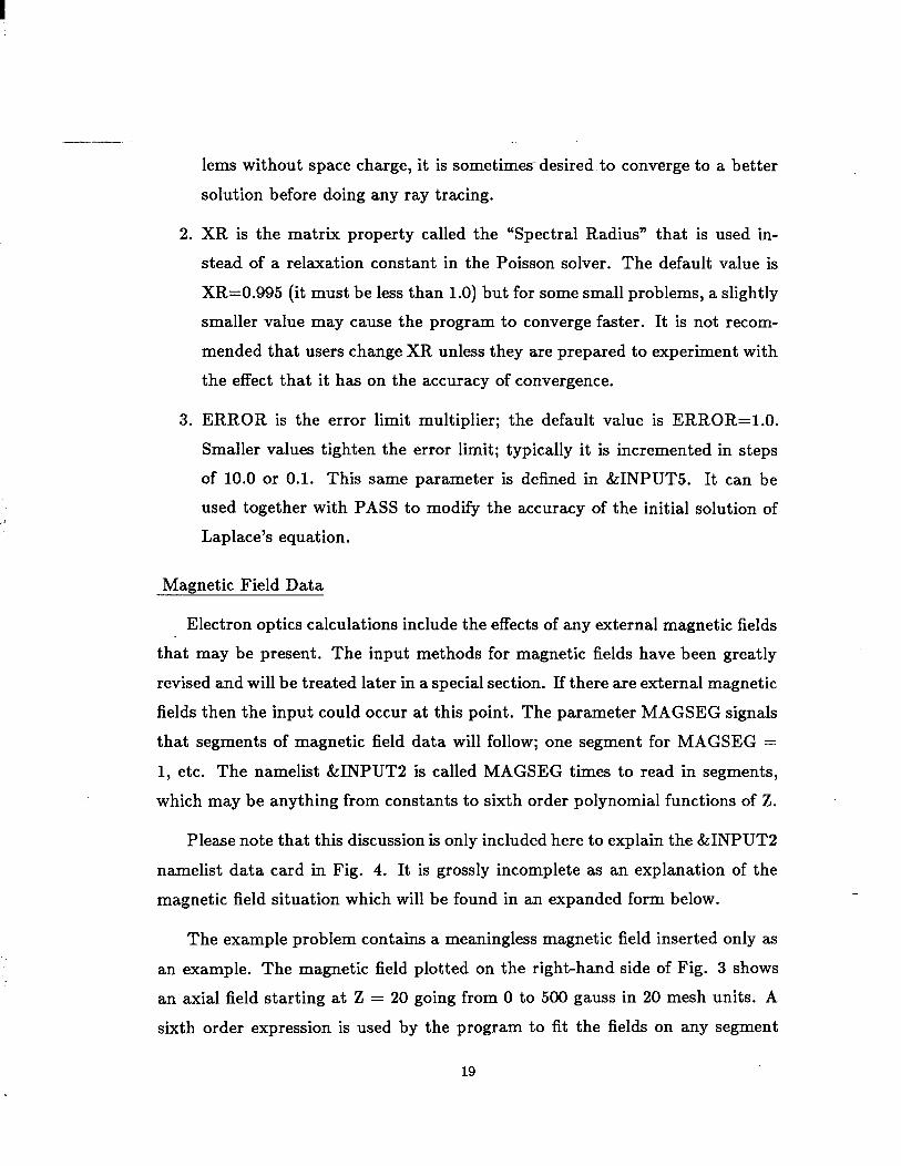
2. XR is the matrix property called the “Spectral Radius” that is used in-

stead of a relaxation constant in the Poisson solver. The default value is

XR=0.995 (it must be less than 1.0) but for some small problems, a slightly

smaller value may cause the program to converge faster. It is not recom-

mended that users change XR unless they are prepared to experiment with

the effect that it has on the accuracy of convergence.

3. ERROR is the error limit multiplier; the default value is ERROR=l.O.

Smaller values tighten the error limit; typically it is incremented in steps

of 10.0 or 0.1. This same parameter is defined in &INPUTS. It can be

used together with PASS to modify the accuracy of the initial solution of

Laplace’s equation.

Magnetic Field Data

Electron optics calculations include the effects of any external magnetic fields

that may be present. The input methods for magnetic fields have been greatly

revised and will be treated later in a special section. If there are external magnetic

fields then the input could occur at this point. The parameter MAGSEG signals

that segments of magnetic field data will follow; one segment for MAGSEG =

1, etc. The namelist &INPUT2 is called MAGSEG times to read in segments,

which may be anything from constants to sixth order polynomial functions of Z.

Please note that this discussion is only included here to explain the &INPUT2

namelist data card in Fig. 4. It is grossly incomplete as an explanation of the

magnetic field situation which will be found in an expanded form below.

The example problem contains a meaningless magnetic field inserted only as

an example. The magnetic field plotted on the right-hand side of Fig. 3 shows

an axial field starting at Z = 20 going from 0 to 500 gauss in 20 mesh units. A

sixth order expression is used by the program to fit the fields on any segment

19

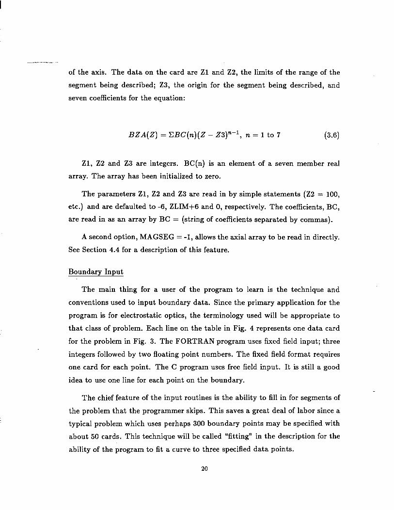
of the axis. The data on t-he card are Zl and Z2, the limits of the range of the

segment being described; 23, the origin for the segment being described, and

seven coefficients for the equation:

BZA(Z) = CBC(n)(Z - Z3)n-1, n = 1 to 7 (3.6)

Zl, 22 and 23 are integers. BC(n) is an element of a seven member real

array. The array has been initialized to zero.

The parameters Zl, 22 and 23 are read in by simple statements (22 = 100,

etc.) and are defaulted to -6, ZLIM+G and 0, respectively. The coefficients, BC,

are read in as an array by BC = (string of coefficients separated by commas).

A second option, MAGSEG = -1, allows the axial array to be read in directly.

See Section 4.4 for a description of this feature.

Boundary Input

The main thing for a user of the program to learn is the technique and

conventions used to input boundary data. Since the primary application for the

program is for electrostatic optics, the terminology used will be appropriate to

that class of problem. Each line on the table in Fig. 4 represents one data card

for the problem in Fig. 3. The FORTRAN program uses fixed field input; three

integers followed by two floating point numbers. The fixed field format requires

one card for each point. The C program uses free field input. It is still a good

idea to use one line for each point on the boundary.

The chief feature of the input routines is the ability to fill in for segments of

the problem that the programmer skips. This saves a great deal of labor since a

typical problem which uses perhaps 300 boundary points may be specified with

about 50 cards. This technique will be called “fitting” in the description for the

ability of the program to fit a curve to three specified data points.

20

Two types of boundaries are used: Dirichlet-boundaries are those on which

the potential is known. Neumann boundaries are those on which the normal

derivative of the potential is known.

Dirichlet boundaries are used to represent metal surfaces. Neumann bound-

aries represent gaps between surfaces and must be chosen so that the normal

component of the field is zero since that is the only value that is ever known in

practice. Thus the cathode is a Dirichlet boundary and the axis is a Neumann

boundary in a typical example. Neumann boundaries can meet at a corner.

For electrostatic problems it has been found satisfactory to restrict Neumann

boundaries to lie along mesh lines. Dirichlet boundaries may have any shape

desired although the mesh spacing limits the resolution of the smallest details

which can be effectively used. Slanted Neumann boundaries are possible however,

and the input technique will be described later in this section.

A boundary point is defined as any mesh point less than one mesh unit from

the boundary of the problem, but always within the boundary. The points on

a Neumann boundary are always boundary points. The points on a Dirichlet

boundary are never boundary points. This difference, which is inherent in the

formulation and not just a program convention, gives rise to a code to determine

which type boundary is being specified. Thus, if the distance from a point to a

boundary in either the R or Z direction is zero, then that boundary is defined as

a Neumann boundary.

There are five entries on each boundary data card;

1. Potential number, integer, corresponds to the surface numbers denoting

elements of the array POT(I) described earlier.

2. R, integer, the value of the radial coordinate of the mesh at the boundary

point.

3. Z, integer, the value of the axial coordinate of the mesh at the boundary

point.

21

4. DELTAR, floating point, the distance from-the mesh point to the boundary

in the radial direction. DELTAR is negative if the boundary intersects the

radial line at a point in the minus direction from the mesh point. If the

intersection is greater than one mesh unit from the boundary point then

the intersection is not significant. Any number greater than 1.0 could be

used but typically the distance is specified as 2.0 if it is greater than 1.0.

5. DELTAZ, floating point, the distance from the mesh point to the boundary

in the Z or axial direction. The same rules as for DELTAR, above, apply.

In the case of a point on a Neumann boundary, the potential number is

not significant. If the point is simultaneously within one mesh unit of a Dirichlet

boundary, then the potential number is the number for that surface. Otherwise it

is customary to punch a zero for the potential number. It is important to realize

that a zero for the potential number is not the code number for a Neumann

boundary. Repeating, the code for a Neumann boundary is a zero for DELTAR

if the boundary is parallel to the azis. If the boundary is a radial plane, then the

code is DELTAZ = 0.

A mesh point cannot simultaneously be a boundary point for two Dirichlet

surfaces at different potentials. This is not usually a problem for the programmer.

However, there can be situations when it is necessary to make some adjustment

in the problem to avoid a situation in which, either DELTAR or DELTAZ should

have two values, or in which DELTAR and DELTAZ refer to two different surfaces

in which neither is a Neumann boundary.

Note that this also means that a single point cannot be a complete row or

a complete column. A column must have a top point and a bottom point, each

of which has a DELTAR between -1.0 and +l.O. Since one point cannot have

both of these, one point cannot be a column. The same thing applies to rows.

However, the program applies tests for the columns only.

Boundary points must be defined in sequential order. Adjacent points must

be within one mesh unit in both R and Z. If a boundary point is not within one

22

-- -

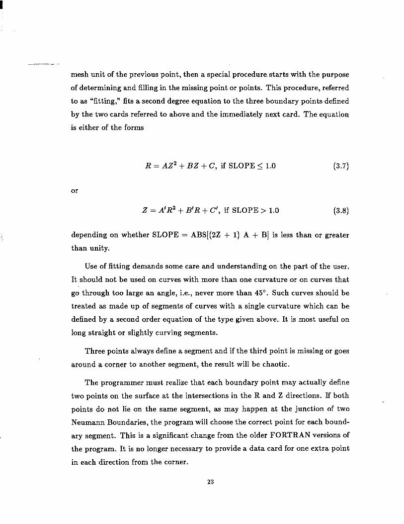
mesh unit of the previous point, then a special procedurastarts with the purpose

of determining and filling in the missing point or points. This procedure, referred

to as “fitting,” fits a second degree equation to the three boundary points defined

by the two cards referred to above and the immediately next card. The equation

is either of the forms

R = AZ2 + BZ + C, if SLOPE 5 1.0

or

Z = A’R2 + B’R + C’, if SLOPE > 1.0

(3.7)

depending on whether SLOPE = ABS[(2Z + 1) A + B] is less than or greater

than unity.

Use of fitting demands some care and understanding on the part of the user.

It should not be used on curves with more than one curvature or on curves that

go through too large an angle, i.e., never more than 45’. Such curves should be

treated as made up of segments of curves with a single curvature which can be

defined by a second order equation of the type given above. It is most useful on

long straight or slightly curving segments.

Three points always define a segment and if the third point is missing or goes

around a corner to another segment, the result will be chaotic.

The programmer must realize that each boundary point may actually define

two points on the surface at the intersections in the R and Z directions. If both

points do not lie on the same segment, as may happen at the junction of two

Neumann Boundaries, the program will choose the correct point for each bound-

ary segment. This is a significant change from the older FORTRAN versions of

the program. It is no longer necessary to provide a data card for one extra point

in each direction from the corner.

23

In the special, but quite common, case in which one of- the surfaces at a

corner is a Neumann boundary, the potential number refers to the conducting

boundary and the Neumann boundary is defined by an appropriate entry of 0.0

for either DELTAR or DELTAZ. Beginners should clearly understand this; look

at the example for the first boundary point below to avoid a common mistake

that has frequently been observed in new users.

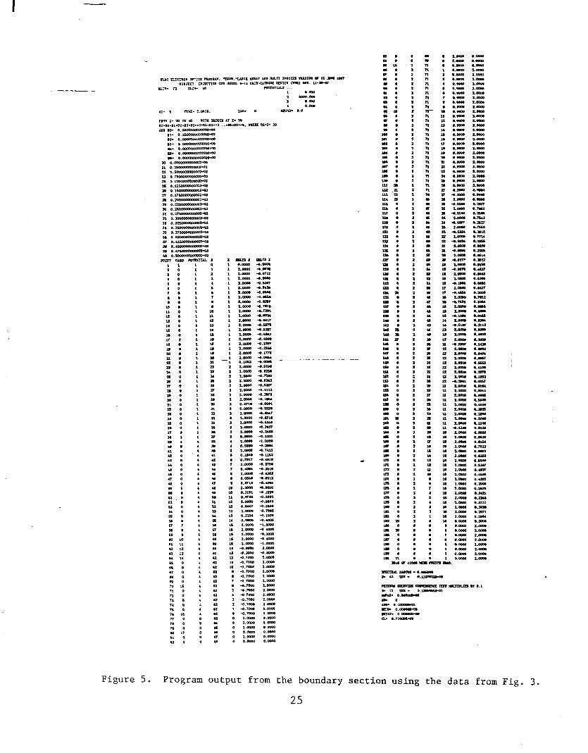
The boundary output listing shown on Fig. 5 will now be examined in detail

as an example. Notice that there are seven columns; POINT, CARD, POTEN-

TIAL, R. Z, DELTAR, DELTAZ. The POINT column is just the point number.

The CARD column contains a sequential number if such a card exists; otherwise

it contains a zero. The remaining columns contain the identical data as are found

on the card, or the data resulting from fitting. It is useful to compare Figs. 3, 4

and 5 as the following discussion progresses.

Card number one: Potential number one, (cathode), R = 0, Z = 1, (this is

the usual starting place), DELTAR = 0.0, (code for Neumann boundary along

the axis), DELTAZ =-0.99, (-1.0 could have been used but 1.0 for the DELTA

terms can result in some confusion for the fitting routine). The point R = 0, Z =

0 could also have been used but it is risky to use -0.01, for example, for DELTAZ

because the curve could try to cross the Z = 0 line before R = 1, thus resulting in

a point with two values of DELTAR, 0.0 and some positive fraction. This would

also have the result of adding another column to the problem without increasing

the resolution or the actual area, thus resulting in a fractional slow down. Thus

0.99 or 0.999 is frequently used for DELTAR or DELTAZ.

24

I.- ..000 : I.- 0.m . Rum ..- : *.- I.- l.oOm :.zz I.- : ..- . a.- :=

Figure 5. Program output from the boundary section using the data from Fig. 3.

25

Card number two: POT = 1, R = 16, Z = 1; DELTAR = 2.6, DELTAZ =-

0.4. Since R = 16 is more than one unit from R = 0 on card one, the automatic

fitting routine will be called. It will read the next card which must also be on

the cathode surface. The DELTAR = 2.0 indicates that the boundary does not

cross within one mesh unit in the R direction. Card number three: POT = 1, R

= 37, Z = 3, DELTAR = 0.99, DELTAZ = -0.1. Both DELTAR and DELTAZ

refer to the same curve segment, so there is no ambiguity for the fitting. The

coordinates of the points through which the curve will fit are: (r = 0, z = O.Ol),

(r = 16.0, z = 0.6) and (r = 37.99, z = 3.0). It will use Eq. (3.8) rather than

Eq. (3.7) because the absolute value of the slope is greater than one.

Card number four: POT = 4, R = 38, Z =4, DELTAR = 2.0, DELTAZ =

-1.0. Pot = 4 is used to permit the focus electrode, which this surface is, to be

distinguished from the cathode. The -1.0 for DELTAZ is inadvisable but works

on the first point of the set of three. No fitting since R and Z are 1 mesh unit

from those on card three.

Card number five: POT = 4, R = 48, Z = 10, DELTAR = 2.0, DELTAZ =

-0.8. This card causes the automatic fitting procedure to be called.

Card number six: POT = 4, R = 55, Z = 15, DELTAR = 0.99, DELTAZ =

-0.6. This is the third card of the set and fits the straight section of the focus

electrode.

The next several cards define the boundary around the point on the focus

electrode. The logic should be obvious by inspection. Fitting is used for the top

of .the focus electrode.

Card number sixteen: POT = 4, R = 62, Z = 0, DELTAR = -0.7, DELTAZ

= 0.0. This card is interesting because it defines the end of the segment to be fit

along the top of the focus electrode and the beginning of the Neumann segment

along Z = 0. Because of the Neumann condition (DELTAZ = 0.0) the program

recognizes the corner condition and fits to the point (r = 61.3, z = 0.0.

26

Card number seventeen: POT = 0, R = 66, Z-= 0, DELTA-R = 2.0, DELTAZ

= 0.0. This is a case where one might forget to skip a point and make R = 63

. . . don’t. Also note especially the DELTAR = 2.0 . . . there is no surface in the

R direction for more than one mesh unit, even though the point lies right on the

Neumann boundary.

Card number eighteen: POT = 2, R = 71, Z = 0, DELTAR = 0.99, DELTAZ

= 0.0. Potential 2 is for the anode, which is the role played by the gun grid

in this example. The 0.0 for DELTAZ signifies the vertical Neumann boundary.

Note that this card is used to begin the next fitting segment.

Card number twenty: POT = 2, R = 71, Z = 27, DELTAR = 0.99, DELTAZ

= 2.0. This is an “extra” card inserted to avoid the corner ambiguity which

would occur if the fitting program had to use the next card which points to two

different line segments of the same surface. Actually, this data card is a vestige

of an old data set; the extra card next to the corner is no longer required.

Cards number twenty-one and twenty-two: POT = 2, R = 71 and R = 70,

Z T 27, DELTAR = 0.99 and 0.2, and DELTAZ = 0.99. These two cards form

a short column to avoid a column of length one at the corner. Clearly they do

not agree with the design surface, but the location is such that the discrepancy

cannot affect the solution.

The last three boundary cards define the Neumann segment on the axis.

Note that the last card, POT = 0, R = 0, Z = 2, DELTAR = 0.0, DELTAZ =

2.0, specifies the point immediately adjacent to the first point, thus completely

defining the boundary. The boundary must be completed in this way without

ever repeating a boundary point.

The next card, with 888 in the POT field, or any other potential number

greater than POTN, terminates the boundary input. If this number is 999, special

boundary conditions are expected to follow in the input file, as explained below.

If there are no special boundary points, then the next step for the program is to

calculate the difference equations and to perform some checks on the boundary

27

data.

Special Boundary Conditions

A curved or slanted Neumann boundary, except for 45’, requires the gen-

eral Neumann conditions as described in Appendix II. The special case of a 45’

Neumann boundary is correctly described if both DELTAR = 0 and DELTAZ =

0. General Neumann and other boundary conditions such as dielectric surfaces,

may be put in as calculated values by overwriting the difference equations calcu-

lated by the program. The normal ending to the boundary data is by a potential

number greater than POTN. If 999 is used, the program will commence reading

cards containing R and Z; the coordinates of an existing boundary point, and

Dl, D2, D3 and D5; the four coefficients of the difference equation for the point

(W).

R and Z are integers locating an existing boundary point. Dl, D2, D3 and D5

are the real positive coefficients of the difference equation at (R,Z). Any number

of such cards may be used in any sequence, An R value greater than RLIM

terminates this input.

Dielectric materials may be simulated by special boundary values at the di-

electric surface. The surface must have been defined as a boundary so that the

points exist in the data file. Usually this can be done with a simple straight

line of dummy boundary points, having DELTAR = DELTAZ = 2.0. The rules

for this are summarized in the condensed instructions and will be explained in

Section 4.9.

Grids

The program can handle electrode structures of remarkable complexity, in-

cluding such arrangements as grids. Of course, in cylindrical symmetry, the grid

can consist only of a set of rings; the radial support wires do not apply. It can

be shown that most of the harm done to a beam by a grid is done by the rings,

28

and that azimuthal deflections that would be caused by-the radial wires are less

significant.

Two kinds of grids are of interest:

1. Ideal grids that consist of a thin electrode, of any arbitrary shape, for which

both sides are defined using ordinary boundary definitions. Such grids are

“ideal” in the sense that there is no field penetration, hence no particle

deflections, and also no particle interception. Trajectories will pass directly

through thin grids because, in general, the ray tracing routines attempt

to continue propagating a particle until the partial differentiation routine

can no longer calculate fields. There is always one iteration step which

crosses the boundary so that the particle finds itself on the other side of

the electrode.

2. The second type of grid is actually made up of individual wires, which as

pointed out above, must extend in the PHI direction in either coordinate

system. In order to resolve individual wires, the mesh density must be

- significantly finer than the grid spacing. Wires must lie on a mesh line in

order to be noticed by the boundary definition. It does not seem to matter

if the grid wires lie on a mesh node or simply lie on one mesh line. If on a

node, then four adjacent points become boundary points defining that grid

wire, while if only on a mesh line, then the two adjacent points define the

wire. The closest meaningful grid spacing would occur if a grid wire lies

on every second horizontal mesh line (for a vertical or nearly vertical grid).

This allows for some field to leak through the space between wires and for

some grid-induced particle deflection to occur. Obviously if the grid wires

are spaced so closely that they have the same spacing as the mesh, then

the simulation results in the definition of the ideal grid described above.

In defining grid wires, it can be necessary to define “dummy” boundary

points in order to make the sequential definition of boundary points from a real

boundary to a grid wire, or between wires, and back again. Dummy boundary

29

points consist simply of boundary points with both DELTAR andDELTAZ=2.0.

It is possible to use boundary fitting for dummy boundaries; the rules are the

same as for Neumann boundaries, that is, the boundary line must lie on a mesh

line. Internally the program will treat dummy boundary points as if they are

ordinary interior points, except that their difference coefficients are found in the

array with all the other boundary points. The boundary plots are apt to be

rather messy looking from such a grid structure. Usually the game in defining

any boundary, especially a complex one with grids, is to do it with the fewest

number of points, hence the least amount of work.

Boundary Diagnostics

If the input data are acceptable, the next message printed on the output

is: SPECTRAL RADIUS=0.995. The spectral radius is a constant used by the

program for the convergence of the solution of Poisson’s equation.

BOUNDARY ERROR IN COLUMN XX

If this message appears somewhere in the middle of the listing of boundary

data, it is a signal that the boundary data have exceeded the limits of the prob-

lem, 0 5 R 5 RLIM and 0 5 2 5 ZLIM, or that the boundary data have

exceeded the maximum number allowed which is presently 1101. Thus, this mes-

sage appears if the boundary calculation goes into a loop. Loops usually result

from an error in boundary fitting as might be caused by omitting one of the three

points of a line segment.

The FORTRAN program will attempt to pick up the boundary computation

and complete the listing even after such an error has been found. However, the

problem will not attempt to run and there may be other errors caused by the

program in trying to interpret the rest of the boundary.

In the PC environment, the interactive nature of boundary input is favored

by having the program stop immediately when this type of boundary error is

found. The program makes a plot file which can be immediately plotted to the

30

monitor screen, and showshow far the boundary-has progressed.Sometimes this

is enough to show where the error is, but if not, then the program output file

can be called up to the terminal and the progress can be charted to a particular

data point.

BOUNDARY ERROR IN COLUMN XX

If this message appears at the end of the boundary listing it indicates that

the program checks have found an error. The program checks are based on the

requirement that each column must have a top and a bottom. Since there can

be more than one segment to a column, the requirement translates to mean that

there must be an even number of ends for each value of Z. An end is defined by a

DELTAR value between +l and -1. Thus the programmer need only determine

why there are not an even number of such points for the indicated column.

Note that there are similar checks which could be made but aren’t. Each

row must have two ends also, but no such check is included. Also obviously a

bottom end must have DELTAR between 0.0 and -1.0, not greater than 0.0. This

and similar boundary mistakes are left to the programmer’s care to prevent or

correct.

CHECK BOUNDARY POINTS . . . .

The CHECK BOUNDARY POINTS messages are warnings that the diag-

nostics has located an unusual condition. These may be perfectly correct points,

but the programmer should examine each such message and satisfy himself why

it has been singled out and that it is indeed correct. These checks are, for exam-

ple, good at detecting sign errors on DELTAR and DELTAZ values. Sometimes

adjacent boundary points have opposite signs, but not usually. The warning

messages do not inhibit operation.

In the C version, all these diagnostic messages appear on the screen during

execution and are also printed in the output listing. Programmers should check

for the warning messages when any new or changed boundary is run for the first

time.

31

BOUNDARY ERROR-OR MI NEGATIVE - . - -

If this message appears at the end of the boundary listing the programmer

must check for messages of the previous two types. If there are none, and he

has set MI negative, then the boundary data have passed the program checks. It

is worthwhile for the programmer to look at the output carefully to catch other

boundary errors. The programmer should also always endeavor to get at least

one plot including equipotential lines of any new geometry. Unsuspected errors

frequently become glaringly obvious on examination of a plot. The optional

printout of the table of potentials caused by LSTPOT > 0, should always be

used for a new or revised boundary configuration.

3.3 POISSON'S EQUATION SOLVER

After reading the boundary input, and before reading the starting conditions,

the program makes the first solution of Poisson’s equation (actually Laplace’s

equation at this point since there is no space charge, hence right-hand side (R.H.)

equals zero). The description of the input data for the example will be interrupted

here for a brief description of the mechanics of the solution of Poisson’s equation.

The program solves the complete set of equations for one column at a time.

Mathematically, a matrix for a column consists of a tridiagonal matrix which

must be solved (inverted) to find values for the potential of each of the points in

one column. To do this, the adjacent columns are assumed to contain “known”

values, and the end points are also “knowns.” That is, either the value is known

or, in the case of a Neumann boundary, the adjacent point is assumed to be

the same as the point being solved since the derivative is zero. The relaxation

method is known as the “semi-iterative Chebyshev” method and is described by

Varga.8

Each column consists of two or more points, with upper and lower end points

being boundary points for which -1.0 5 DELTAR < 1.0 Thus each column has

at the top and bottom a condition, either Neumann or Dirichlet, that permits

32

the program to write a set of n equations in n unknowns for that column. A

column of the problem area defined simply by the value of Z, may have more

than one segment which must each meet the above definition of a “column.”

Each such column must have its proper ends. In the example problem, there are

two columns for each value of Z up to and including Z = 14.

When a column is solved, the adjacent columns are considered fixed. Alter-

nate columns are solved so that on two passes first the odd numbered columns

and then the even numbered columns are solved. After 50 iterations, (25 in the

C program) or less if the error criterion is satisfied, the calculation is stopped

and a message is printed:

N=51, ERR = X.XXE - XX.

This is the signal that after 50 iterations (the counter is already set to 51) the

largest single change of a potential is ERR volts. The convergence criterion can be

adjusted by using the parameter ERROR. The error criterion is automatically

tightened by a factor of ten for the final cycle. Certain problems using large

areas of Neumann boundaries, are subject to slow convergence so that the results

may be incorrect. This can be remedied either by iterating for more cycles or

by giving the program a better starting distribution. The initialization of the

present versions of the program are much superior to those in earler versions.

The FORTRAN program has had the same improvements as have been installed

in the C program, and allow it to seek convergence in two sets of 25 iterative

passes each. Generally the iteration process is quite satisfactory and after 50

iterations the field is sufficiently determined to start ray tracing leading to the

inclusion of space charge.

If the Poisson solver detects that the solution is not converging it will stop

with a message, POISSON EQN FAILS TO CONVERGE. As a general rule, this

means there is a boundary error, but there are at least two situations in which

the user may have to try to fool the test:

1. If a drift tube or structure is simulated with little or no voltage on any

33

electrode, the injection of space charge ‘may trigger the the convergence

message. The cure is to specify a significant positive voltage in the POT

array. The potential does not have to correspond to an element of the array

that is actually used on the boundary.

2. The second condition under which this message may occur is if the Laplace

solution is very slow due to, for example, the large area of Neumann bound-

ary noted above. The cure, if everything else appears okay, is the same as

above; specify a potential that is, for example, ten times larger than the

largest one in the problem.

After finishing the first cycle of Poisson’s equation, a potential map, or

POTLIST, is printed giving the potential (normalized to 100% of the maximum

potential) for every point in the RLIM by ZLIM space. Since this includes back-

ground points (points behind the surfaces) one can usually trace the outline of

the problem. The POTLIST is an exceptionally effective diagnostic device and

should always be studied for peculiarities. An error in boundary data may, for

example, leave a strange zero in the middle of the high potential part of a device,

thereby greatly distorting the fields. When used together with the equipoten-

tial plots, it is possible to pinpoint errors in a few minutes. The POTLIST is

suppressed by setting LSTPOT = 0 in &INPUTl.

34

4. STARTING CONDITIONS

After the first calculation of Poisson’s equation, the program reads the start-

ing conditions. The format is NAMELIST consisting of defining equations in

which the variable is named followed by an “equal” sign and the value. Only

those variables that need to be altered from the default conditions need to be

specified. The sample problem demonstrates how little data needs to be specified

in many cases. Using the sample problem, the following remarks will illustrate

the technique. In the rest of this section, a brief description will be given for each

of the options currently included in the program. Since other options can always

be added, the user must refer to the comments in the program for the up-to-date

implementation.

The sample problem is coded as a spherical diode or Pierce gun. The card

with &INPUT5 signals that the namelist entries follows. The entry START =

‘SPHERE’ directs that the spherical diode conditions will be used. The entries

RAD = 257 and RMAX = 37.5 give the spherical radius and cathode radius

respectively. UNITIN = 0.01 specifies that the scale of the problem is 0.01

inches/mesh unit. All problem scaling is in MKSA units so that UNITIN is

immediately converted to unit in meters. After reading these items the program

prints a table of all the starting parameters.

The starting conditions are described in the following Sections according to

function as follows:

4.1 Universal; apply to more than one case,

4.2 Equipotential lines; controls equipotential plotting,

4.3 Plotting; plot controls,

35

4.4 Magnetic fields; input and calculation parameters for magnetic fields,

4.5 General cathode; parameters controlling the general cathode option,

4.6 Spherical cathode; parameters which specifically apply to the spherical

cathode option.

4.7 Card starting; parameters controlling the use of user specified starting

conditions.

4.8 Laplace starting; parameters controlling the use of the program for ap-

plications other than ray tracing.

4.9 Dielectric Boundaries; how dielectric materials can be included in the

problem specification.

4.1 UNIVERSAL PARAMETERS

For each starting parameter, there is a default value which will be the value

used if it is not changed by the input. In the following discussions, the entries

will be given as described by the program comments with the format:

INSTRUCTION DEFAULT, MAX COMMENT

This will be followed by a discussion of the use of the parameter. The lines

in UPPER CASE are selected verbatim quotes from the Condensed Instructions

which appear in Appendix III. When a second number, separated by a comma,

appears for the default value, it refers to the maximum allowed value, usually

determined by array limits.

PERVO= X.Xx PERVO = 0 ZERO USES LAPLACE/

.- PERVO is the initial value of the perveance of the beam for either the START

= ‘SPHERE’ or START = ‘GENERAL’ methods. Perveance is defined as the

constant K in the expression .

36

I = M x v3i2 x lo6

- .

Here K is expressed in micropervs so that, for example, a microperveance

1.0 device operating at lo4 volts would have a current of 1.0 A. The entry X.Xx

indicates that a decimal number is the expected value. When a single X is used, it

implies that an integer is expected. The X’s do not indicate the input format; the

number of significant figures is not restricted except by the computer hardware,

and by the logic of the program.

PERVO normally controls only the perveance of the first cycle. However,

it may be “held” for any desired number of cycles by using HOLD = X. The

process by which the program determines perveance is to average the perveance

calculated for a given cycle with the perveance actually used in the preceding

cycle. The new averaged value is then used to determine the current per ray.

The averaging process has proven very effective in quickly arriving at a stable

value. It has been so successful that it is frequently better to start with the

averaging method than with a value “known” to be “correct” from experiment

or from prior calculations. The default value PERVO = 0 is a code instruction

which takes the value of perveance calculated for the LAPLACE solution and

simply divides it by two to arrive at the perveance for the first cycle. The new

user of the program is advised to use the default value until specific experiences

lead him to try something else.

HOLD = X HOLD = 1 PERVO ‘HOLDS’ FOR HOLD PROGRAM

CYCLES

HOLD = 2 or more causes the input value of PERVO to remain unchanged .

37

by the averaging process for HOLD program cycles. There are some problems,

particularly with very nonuniform cathode loading, where using HOLD helps

establish the necessary space charge environment for the process to stabilize. A

more frequent application is to simulate temperature limited emission conditions

by running the entire problem with a fixed reduced perveance. Then, of course,

HOLD must be at least as large as NS.

-

PE = X.X PE = 0.1 INITIAL ENERGY AT CATHODE IN EV

PE is the incremental energy that is added to every trajectory to account for

the combined effect of work function potential and thermal energy. Like PERVO

and HOLD, PE is only used for starting with one of the Child’s Law routines

for calculating the initial conditions. It is normally not necessary to have any

initial PE, but some small changes may be observed by varying it. In a few low

emission devices, it has been found essential to have some initial energy to avoid

instabilities near the cathode.

ERROR = X.X ERROR = 1.0 MULTIPLIES ERROR TEST

ERROR multiplies the built in error test by which the program determines

that an adequate solution of Poisson’s equation has been reached. If the problem

is slow to converge, particularly if there are large areas of Neumann boundary,

it may be necessary to reduce the allowed error, e.g., ERROR = 0.1, to get

the program to converge at all. Slow convergence is indicated if each cycle only

iterates three times, prints N = 3, ERR = nnn, and calculates the trajectories.

On the last cycle, the error test is reduced by a factor of 10 from whatever level -

- was set by the user. Some hints about convergence problems will be found in

a later section. The ERR value returned by the program is the largest single

change of any mesh point during the last iterative cycle, in volts. .

38

UNIT = X.XxX UNIT = 0.001 METERS/MESH UNIT

UNITIN = X.XxX (SEE UNIT) INCHES/MESH UNIT

The default scale value for the program is 0.001 meters/mesh unit. If a value

is given for UNITIN (’ h / mc es mesh unit) this value will be immediately converted

to meters. Except for problems using magnetic fields, the optics of an electron

gun does not depend on the scale factor. All the standard rules of scaling in

electron optics can be used once a problem has been solved.

LSTRH = X LSTRH = 0 IF>O, PRINTS SPACE CHARGE MAP

This option is mostly used as a diagnostic for program debugging. It prints

a map of deposited space charge with the same format as the POTLST map of

potentials.

MAXRAY = XX MAXRAY = 27,101 MAXIMUM NUMBER OF RAYS

If MAXRAY IS NEGATIVE, THE NUMBER OF RAYS=ABS(MAXRAY)

MAXRAY determines the maximum number of electron trajectories that can

be calculated. The arrays for trajectories have a limit of 101. The number of

rays used by START = ‘GENERAL’ or START = ‘SPHERE’ is determined by

a program algorithm unless the value of MAXRAY is negative. Within the limit

MAXRAY, the program tries to make the largest possible integral number of

rays per mesh unit at the cathode.

STEP = O.XX STEP = 0.8 MESH UNITS/STEP

STEP is the iteration step length for ray tracing. It must be less than 1.0

- ---- for the program to properly account for space charge, calculate magnetic fields,

etc., when crossing a mesh line. The equations of motion are time dependent,

thus the program uses STEP to calculate step time from the velocity at the start .

39

of the step. Since the electron can accelerate during a step, it may may actually

go slightly farther than STEP. The default value is about the largest that should

be used. If magnetic fields are present, STEP should usually be reduced at least

a factor of two. On the last cycle, STEP is automatically reduced by a factor

of two. Shortening the step means more time will be required for a problem.

As a rule of thumb, the program spends roughly half of the time with Poisson’s

equation and half with the ray tracing. Thus reducing STEP by a factor of two

could increase running time by about 25%. The Runge-Kutta method is used

to solve the differential equations of motion. Because of the necessity to take

small steps anyway, and because of the time needed, the program does not use

any of the “predictor-corrector” techniques of verifying step length. Experience

has shown that errors due to STEP being too large, especially if magnetic fields

are included, become glaringly obvious when the plots are examined. The most

frequent effect is for a trajectory to get too close to the axis, violate conservation

of angular momentum in one step, and fly out of the problem area with /3 > 1.0,

where p = V/C. An error message is printed when a ray ends with ,0 > 1.0. At

the very least, this is a signal to reduce STEP in subsequent runs.

NS = X NS = 7 NUMBER OF PROGRAM CYCLES

NS defines the number of program cycles to be made. In the program, NL

is used as the running variable to record the number of cycles left to be run.

Initially NL = NS. The default value is usually acceptable unless the program

is having trouble converging on the perveance. For the special case of no space

-.-- charge, it is advisable to still use NS = 2 to gain the insight afforded by the

reduction of ERROR and STEP on the final cycle. For START = ‘LAPLACE’,

NS is the number of times that Laplace’s equation will be cycled.

40

SPC=X.X SPC=O.5 ESTIMATED SPACE CHARGE

SPC SIMULATES PARAXIAL APPROXIMATION ON FIRST CYCLE.

SPC IS THE FRACTION OF THE RADIAL FORCE USED.

SPC = 1 FOR FULL EFFECT, SPC = 0 FOR NO EFFECT.

SPC determines the fraction of the ordinary radial electrostatic force that

will be applied to the rays on the first cycle. In a device in which space charge

forces play a strong part in the focusing, the external electrostatic fields usually

have a strong radial focusing effect. If not opposed by space charge on the first

cycle, these forces may cause the rays to strongly over focus leading to a poor

initial distribution of the space charge. The full contribution, SPC = 1.0, adds a

term to the radial equation of motion simulating all the current, of all the rays

calculated, to lie in a conductor on the axis. Thus it is assumed that the rays are

calculated in sequence starting with the ray nearest to the axis. In the case of an

electron gun calculation starting at the cathode and extending infinitely in only

one direction, a better choice is SPC=O.5 which attenuates the radial force by

0.5. Further from the cathode, SPC = 0.5 is a less logical choice, but the beam

is less sensitive to radial forces as it gains in energy. Empirically, it has been

found that SPC = 0.5 is a good choice for gun problems involving starting from

the cathode. For other types of problems, the user should be aware of the fact

that SPC exists and can be changed. In rectangular coordinates, SPC simulates

an infinite sheet of current on the axis. If the problem does not involve reflection

about the R = 0 plane, then there is a transverse force (which does not depend

._ on distance from the x-axis) which should be turned off by SPC = 0.0. Since

SPC only affects the first cycle, the program will usually forgive any misuse of

it. SPC can be useful in arriving at a satisfactory solution of one usually difficult

41

problem, that of a long thin beam with magnetic fields providing the focusing.

This can be a difficult problem to get to stabilize because of the poor aspect ratio

which frequently finds a large fraction of the beam within one or two mesh units

of the axis. However, it is usually well represented by the paraxial approximation

so that a single cycle run, NS = 1, with SPC = 1, will frequently result in a good

solution. In this case one must be sure that STEP is small enough and that an

adequate solution of Laplace’s equation was attained.

PHILIM = X.X PHILIM = 0.0 AZIMUTHAL LIMIT

PHILIM .NE. 0 ENDS TRAJECTORY AT PHI .GT. PHILIM

For special applications, it is possible to establish an orbit that would continue

until the program is stopped. An example is an electron orbiting in a uniform

magnetic field. PHILIM has the units of PHI; radians in cylindrical coordinates

and mesh units in rectangular coordinates.

SAVE =l SAVE = 0 SAVE = 1 SAVES BOUNDARIES

TO USE SAVE = 1, OMIT BOUNDARY CARDS FROM NEXT PROBLEM

SAVE = 1 is a signal to the program to expect a second problem run imme-

diately after the first problem, and that the second problem will use the same

boundary conditions. It is always possible tobrun tandem problems although, at

most computer facilities, there is no particular incentive to do so. Programs are

usually run from load modules, or from a library of compiled subroutines to be

linked with very little expense, and separate problems can be run independently

without the risk that a failure in the first problem will affect or knock out the sec-

- ond one. However, in the case where successive problems use the same boundary

conditions, considerable savings in effort and computer time can result by saving

the boundaries, which also saves the arrays of potentials and space charge.

42

The SAVE = 1 parameter is put in the starting conditions of the first problem,

not the second one unless there is still to be a third problem. The data deck for

the second problem starts immediately after the last data card of the first deck

with no control cards. The second deck is complete in every respect including

title, potential, magnetic fields, etc., except that the boundary cards and the

accompanying large potential number card are omitted. The potentials can be

changed between runs; if the largest potential is changed, the program will scale

all potentials in the potential map proportionately. Otherwise the program will

start out just as if a cold start was being made, except that the old solution,

including the last space charge array, is used as a “preload.”

One example of the use of SAVE is to be able to trace rays with small

changes of either voltage or magnetic fields. Another use is in the case in which

the Laplace solution is difficult to achieve because of extended lengths of Neu-

mann boundaries. In this case, it may help to run the first part with START =

‘LAPLACE’ and SAVE = 1 and then do the ray tracing in the following problem.

This saves the time and expense of doing ray tracing in an incorrect potential

distribution. This procedure is not normally required since the usual procedure

allows the program to improve the solution on successive iterations as the space

charge is entered. Note that the PC program has input items in &INPUT1

that allow the user to obtain a better solution of Laplace’s equation using the

parameters PASS and ERROR.

In older FORTRAN versions of EGUN, the special case of a pair of elec-

-- trodes separated by a long length of Neumann boundary parallel to the z-axis

causes special problems with convergence that might respond to the approach

using START = ‘LAPLACE’. An alternative method, which is easier, is to intro-

43

duce a few boundary points along the top or bottom Neumann boundaries, with

potential numbers. If the corresponding voltages, which must be entered in the

potential list, represent approximate values for the potentials in the final solution

at that point, then the starting load to the program will be much better than the

normal starting load. Usually the starting load is of very little significance, but

in this special case it can be crucial. The special boundary points are exactly like

the usual Neumann points, except that the potential number is given and refers

to an appropriate element of the POT array. After the preload, the Neumann

points relax as usual and the potentials change accordingly.

In the newer versions of the program (both FORTRAN and C), a better built-

in preload routine senses the desired potentials at the left and right hand ends

of each row, or row segment, and linearly interpolates the starting potentials.

In a problem with Neumann boundaries at one end of a row, and large areas

of Neumann surface in general, it may still be sometimes useful to employ the

above strategy.

SAVE = 2 SAVE = 0 USES FINAL DATA

FROM PREVIOUS RUN TO START THIS RUN.

USE ONLY WHEN START = ‘CARDS’.

SAVE = 2 allows consecutive runs to use the final conditions of a preceding

problem as the initial conditions of the succeeding problem. Necessary scaling

and positioning adjustments are made as described under START = ‘CARDS’,

-- below. The SAVE = 2 goes in &INPUT5 of the second run.

The dual use of SAVE = 1 and SAVE = 2 in one problem is possible and is

signaled by SAVE = 3. It is more common to use SAVE = 1 on the first problem .

44

followed by SAVE = 2 in the second. SAVE = 3 simulates the repeated use of a

drift tube, periodic focusing section, etc.

MASS = X.X MASS = 0.0 MASS > 0 FOR IONS

MASS IS THE MASS TO CHARGE RATIO, 1.0 FOR PROTONS

USE NEGATIVE VALUES OF MASS FOR RAYS WITHOUT INERTIA;

LIKE IN MOLASSES, CAN BE USED FOR MAGNETIC FLUX LINES

OR ELECTRIC FIELD LINES.

MASS is used to signal the program that particles other than electrons are

to be followed. The units are in 1836 electron masses, so that a proton would

be 1.0 and a doubly ionized tritium ion would be 3/2 = 1.5, for example. The

Child’s Law routines for starting still function. Note that the intrinsic charge

built into the program is negative. Ion problems are normally run as if charge is

negative, although negative current (positive charges) are permitted for START

= ‘CARDS’. See the discussion about multiple species with different masses in

the section on START=‘CARDS’.

AV = X AV = 0 SPACE CHARGE AVERAGED LAST AV CYCLES

AVR = X.X AVR = 1.0 WEIGHT OF SPACE CHARGE

IN PRECEDING PROGRAM CYCLE FOR AV.

AV and AVR are companion parameters to help improve stability by aver-

aging the contribution of space charge over successive cycles. It should not be

confused with the different process of emission averaging. In fact, to keep the

-- emission averaging and space charge averaging from affecting each other, it is

suggested that AV be small enough so that the emission averaging is essentially

complete before space charge averaging starts. Note that AV is for the last AV .

45

cycles, e.g., if NS = 7 and AV = 3, then only cycles 5, 6 and 7 are averaged.

However, this may have a very small effect since the -trajectory calculations of

cycle 5 are not affected and the space charge determined by the cycle 7 is never

used (since there is no cycle 8). Thus the effect of averaging is only observed for

AV-1 cycles. AVR determines the weight of the previous cycle such that with

AVR = 1.0, the space charge from the previous cycle is weighted equally with

the present cycle. AVR can have any value, 0 < AVR < co.

Experience with averaging has shown the effect to be less dramatic than

one might anticipate. A poorly designed gun, with strong spherical aberrations

and resulting crossovers, is likely to be unstable and converge poorly even with

averaging. Also, application of averaging to relativistic high intensity beams

does not do much to solve the inherent difficulty caused by the fact that the

self-magnetic field forces nearly cancel the space charge forces. With the two-

cycle format of the program (i.e., space charge from the previous cycle and self-

fields from the present cycle) the program has difficulty converging on long beam

transport problems. The solution to this situation is frequently to use the first

cycle only with the paraxial approximation and SPC = 1.0 as described above.

Even better in many cases, is the new feature using the parameter ZDOTEQ,

described below.

BEND = X.X BEND = 0.0 MAGNETIC BENDING FIELD IN

GAUSS IN THE DIRECTION NORMAL TO THE R-Z PLANE FOR

AXIALLY SYMMETRIC PROBLEMS. FIELD MUST BE UNIFORM.

This feature is most useful for problems with little or no space charge, and is

intended to simulate effects of stray magnetic fields. Various types of photo tubes

have tight tolerance for transverse magnetic field effects. Residual transverse

46

fields, earth’s field, etc., can be calculated. Note that a cylindrical beam in a

rectangular coordinate geometry, including transversefield and space charge, can

be simulated as described below.

MAGMLT = X.X MAGMLT = 1.0 MULTIPLIES BZA ARRAY

MAGMLT multiplies the entire BZA( ) array after it has been read in or

calculated internally. It also multiplies the entire vector potential array if that

option is used. It can be thought of as a knob on all the magnetic field generating

power supplies.

IPBP = Kl, K2,...K6 IPBP= 0 UP TO SIX RAY NUMBERS

FOR POINT-BY-POINT PRINTOUT:

K, RHO, ZETA, RDOT, ZDOT, TDOT, PHI, BR, BZ, STEP, BPHI

In special situations, especially when program behavior is not as expected,

it is useful to be able to print out every iterative step. This feature operates on

the last program cycle. Thus if for example a bug is stopping the program in

the first cycle, it is necessary to set NS = 1 and set IPBP = (the number of the

trajectory at question). Note that it is possible to generate a great deal of paper

this way. In some cases, one might rather have other items printed than those in

the above list. It is a simple change to substitute ER, EZ, etc., for BR, BZ, for

example.

ZEND = X.X ZEND = 1000.0 EXACT END OF TRAJECTORY

CAUTION: IF ZEND IS NOT THE RIGHT-HAND BOUNDARY, THE

- SPACE CHARGE DISTRIBUTION MAY BE INCORRECT.

Normally a trajectory is calculated until the program can no longer determine

the electric fields. Thus the trajectories usually go up to one-half mesh unit

47

beyond the boundaries. In special situations, such as high-resolution photo tubes,

this makes exact interpretation of the results difficult. Setting ZEND to a specific

value causes the program to back up to this value when a trajectory passes

through this value of zeta. This feature can be useful when a particle is still

being accelerated as it strikes the end wall of a device. The acceleration into

metal causes the final energy to be higher than is physically possible, but the

ZEND option can stop the ray at the surface.

VION = X.X VION=-lE8 LOWEST POTENTIAL PERMITTED

USE VION TO SIMULATE SPACE CHARGE NEUTRALIZATION.

Space charge depression can be reduced in a real device by positive ions in an

electron beam or by electron clouds in an ion beam. Since the program normally

runs with negative charges, the above cases both result in negative space charge

depression. If it is desired to limit the depression, VION can be set to the lowest

depressed potential that is desired. The default value is intended to be low

enough so that it will never inadvertently disturb a practical problem.

ZDOTEQ=O.l-1.0 ZDOTEQ=l.O LEVEL TO ENTER EBQ MODE

The EBQ mode is a new EGN feature which allows the program to operate

in the mode in which self magnetic field is accounted for by reducing the space

charge by a factor (l-ZDOT*ZDOT), where ZDOT=v,/c. The choice of the

name EBQ comes from the program of that name written by Art Paul of LLNL.

Users of EGN who have found instabilities with long, thin semi-relativistic beams

should find setting ZDOTEQ at a velocity level below that of their beam, should

give improved results. Some explanation of why this feature is so special, and

what took so long, may be useful. The primary purpose of this program is gun

design, meaning finding the space charge limited current and optics from a gun.

48

Any change of space charge forces must preserve that purpose. The EBQ mode

test is made on every time step of every particle, checking that velocity, ZDOT,

does not exceed the level ZDOTEQ. If it does, then for that trajectory, in only

that part where ZDOT>ZDOTEQ, the self magnetic field field is set to zero and

the space charge deposited is reduced. The intent of this is to solve the problem

of thin relativistic beams, and also to still function in an electron gun if the value

ZDOTEQ is carefully chosen. The idea is to set ZDOTEQ to a value appropriate

to the drift tube, (see the final printout column for values of ZDOT), where the

longitudinal electric fields become negligible and the transverse focusing becomes

a balance of forces between self magnetic fields and space charge. Users should

consider this feature as a knob to experiment with.

4.2 EQUIPOTENTIAL PLOTS

INPUT FOR EQUIPOTENTIAL PLOTS,

The instructions list the parameters which may be used to control the output

of the equipotential lines.

If the plot control parameter MI, on the potential card, has been set to

MI 5 6, then the subroutines which draw equipotential lines will be called at

the appropriate times. If the entire problem is at one potential, it is usually

better not to call for equipotential plots.

The method used in the program to find the equipotential lines consists of

first finding a starting point for the potential to be followed, and then following

- a line of constant potential from that point. This does not guarantee that every

point of that potential will necessarily be found and plotted. If POT (2)# 0, the

program always draws the equipotential line for V = bx POT (2) where b = .

49

0.05, 0.15, 0.25, 0.,35, . . . 0.95. Also if POT (3)# 0, the program draws lines for

V=bxPOT(3) h w ere b = 0.2, 0.4, 0.6,0.8, 1.0. Normally the lines are started

at the points on the axis which are at that potential. The expectation is that

POT (2) will b e used for the anode and POT (3) will be used for the grid, if any.

If, for example, one is designing a gridded gun to be operated at VG = 0.01 VA,

then, by first designing the gun as a diode, and plotting POT (3) at 0.01 POT

(2), one gets the ideal contour for the grid to be electrically invisible.

EQUIPR = X.X EQUIPR = 0.0 R-INTERSECT. FOR EQUIP. LINES

EQUIPR is the radius of the line along which the program hunts for the

potentials which are to be plotted. It sometimes happens, particularly in rectan-

gular coordinates, that the equipotential lines do not intersect the z-axis, (R =

0 line). EQUIPR lets the programmer indicate along which horizontal line the

program should look for the starting points.

LM = XXX LM = 303 LENGTH OF EQUIPOTENTIALS

LM is the array limit for the points to be plotted for any one equipotential. If

a line simply stops in midstream, it may be desired to increase LM. Note that sur-

faces with POT(4), 14, 24, etc., which stop trajectories, also cause equipotentials

to stop when they get near one of these potentials.

EQLN = 0 to 20 EQLN = 1 NO. OF CORRECTIONS

EQLN controls the iterative corrections made as each point is found along

the equipotential line These corrections prevent the lines from deviating from

- sharply curving equipotential lines. The default value, EQLN = 1, is usually

adequate.

EQST = X EQST = 2 STEPS PER MESH UNIT

50

EQST gives the density of points for the equipotential plots. The maximum

length of a line is given by the ratio LM/EQST. If EQST is too small (steps too

long), fine detail may be smoothed over.

ALSO APPLIED TO GENERAL CATHODE

This footnote warns that the starting surface for the GENERAL CATHODE

routine is generated just like an equipotential (but is not plotted), and thus

the parameters EQLN and EQST may determine the accuracy of the starting

surface. It is primarily for this application that EQLN and EQST are made

variable parameters.

IZl = x, IZ2 = x, IZS = x IZl = 0, IZ2 = -1, IZS = 10,

EXTRA EQUIPOTENTIALS AT THE INDICATED VALUES OF Z.

IZl and IZ2 are the end points of a line segment, at EQUIPR, along which

some extra equipotential lines will be started. The lines will be equally spaced

by IZS, instead of by voltage, so that their density will not mean field gradient.

The default value, IZ2 = -1, turns this device off.

4.3 PLOTTING CONTROLS

SCALE = ‘YES’ SCALE = ‘ ’ ‘YES’=DIFFERENT X,Y SCALES

SCALE = ‘YES’ allows the axis routines to adjust both the X and Y scales to

take maximum advantage of the size of the paper. The default value constrains

the axis to have the same scale factor in both directions, thus preserving the

- actual proportions. Using SCALE = ‘YES’ allows the plots to show more detail

between trajectories in problems with low height/length ratios.

SX = XX SX = 22 MAX. HORIZ. PLOT LENGTH

51

SY=XX SY=9 MAX VERTICAL PLOT HEIGHT

The default values are SX=8.5, SY=6 for the EGN87c program. SX and SY

control the area for each picture. The dimensions are given in inches. SX can be

adjusted to suit the length of a given problem.

Plot data generated by the program are stored on an external file (disk) in

a format very similar to that normally used as input to the software supplied

with CALCOMP plotters. A separate job, or second job step, can then be run

to generate the plots. A simple program is printed in the program to convert

these data to make CALCOMP plots. Other plotter software such as that used

at Stanford can be programmed by making the appropriate calls to the local

subroutines. With the changes that resulted in the above system, a programmer

at another installation does not need to search for plotting commands within

the electron trajectory program. Conversion to local software is usually quite

simplified.

For the PC program, a special set of plotting routines is supplied with the

program. If the C program is to be used on something besides a PC, then an

Ascii file is generated which can be read by another plotting routine.

4.4 MAGNETIC FIELDS

Magnetic fields play a vital role in steering and focusing many kinds of elec-

tron beam devices. The capabilities and limitations of the magnetic field imple-

mentation in the program will be described in this section. The following areas

- will be discussed.

1. Magnetic Field Input; (a) axial, (b) ‘d 1 1 ea coils, (c) vector potential data;

2. Off-axis field expansions in Cylindrical Coordinates.

52

3. Magnetic fields in Rectangular Coordinates.

Magnetic Field Input

In the present implementation of the program, there are five methods of

inputting magnetic field data:

1. By reading in the field on the axis using polynomial expansion.

2. By reading the full array fields on the axis, presumably as found by using

another computer program.

3. By reading in vector potential data from the output of a two-dimensional

magnet design program such as TRIM or POISSON.

4. By specifying ideal coils (radius, position and strength). The coils, which

can be wires if in Rectangular coordinates, are then used to find the array

of fields on the axis.

5. The coils, as noted above, can be used with built-in elliptic integral rou-

tines to calculate fields that are valid anywhere, including very near to, or

at higher radius than, the coils. The elliptic integrals can only be used in

cylindrical symmetry, but this method has been used with a very large de-

pressed axis, IAX, which is equivalent to being in Rectangular coordinates.

Description of Axial Magnetic Field

The data cards for an axial magnetic field are put in before the boundary

data. The format was briefly described in Section 3.2. The input data for the

polynomial method consist of MAGSEG segments of data including: ‘Zl’ to

‘22’ with origin at ‘23’ (three integers) and an array BC consisting of the seven

coefficients, BZ, Bl, B2,..., B6; for the expression;

53

B=BZ+B1xDZ+B2xDZ2+...+-B6xDZ6,

where DZ = Z - 23. For the sixth order expansion, the field must start six units

behind the cathode or starting point, and go six units past ZLIM.

The NAMELIST &INPUT1 includes the parameter MAGSEG which deter-

mines how many segments are to be read, each with &INPUT2 and &END cards.

Each segment consists of the data for Zl, 22 and 23 followed by the array BC in

NAMELIST format. The example of the problem input in Fig. 4 shows how this

data is formatted. Zl and 22 are the end points of a line segment on the axis,

where (Zl 5 22) in the range -6 5 Zl, 22 5 ZLIM + 6. It is necessary to permit

fields to be described beyond the ends of the problem in order that the off-axis

fields can be calculated at the ends of the problem. 23 is the local origin for the

polynomial expansion in powers of DZ = Z - 23. Having a local origin simplifies

the input of, for example, a straight line which does not go through (0,O). As

many of the coefficients BZ, Bl, etc., can be used as are necessary, simply by

setting the remaining ones to zero.

In cylindrical coordinates, the field must be in the axial direction. In rectan-

gular coordinates, the default direction for the magnetic field is in the direction

normal to the plane of the plot, i.e., in the PHI direction, where PHI is the

orthogonal linear coordinate to R and Z, or in the R (vertical) direction.

With the above format, data can be entered with any degree of polynomial

- up to 6. Caution is advised if the data handling is done in the following typical

style. The data may be divided into segments ranging from a point at a time

to the whole length of the problem. Typically, magnetic measurements of an

54

axially symmetric permanent magnet will be taken on the axis. The data can

then be smoothed by a polynomial least squares fitting-program and the resulting

coefficients read into the program. Alternatively, a field may be designated by

the user as in the example problem, segmented into short lengths of quadratic or

linear dependence, and read in to the program. Either method will usually give

a good representation of the fields on the axis. The difficulties arise when the

program needs to calculate the off-axis fields. These will be described below.

A separate provision allows one to read in the BZA array directly. Note that

this array starts with BZA(l) at Z = -6 and goes to BZA(ZLIM + 13) at Z

= ZLIM + 6. The program switches to this mode by having MAGSEG < 0,

i.e., if MAGSEG = -1, then a different NAMELIST, &INPUTS, is called to read

the array BZA(). If measured and/or plotted data are used, note especially the

inherent risks in expanding such data for the off-axis field components. This

format lends itself readily to computer calculated output, properly edited, and

with up to 15 effective decimal digits. With an appropriate computer model, for

example, for a set of solenoid coils, this is the most general accurate way to put

in fields. See the book by Montgomery9 for a complete treatment of solenoid

design.

In many cases, a set of ideal point coils can be defined to generate the fields.

The data consists of radius, z-position and strength of up to 101 coils. The

position does not have to be within the RLIM by ZLIM area, and in fact, probably

should not be. Unless it is planned to use the elliptic integral routines, described

below, the off axis expansions break down if magnetic elements lie within the area

of the expansion. The data for ideal coils are read in as part of the &INPUT5

starting conditions.

55

The starting conditions pertaining to magnetic fields are as follows:

MAGNETIC FIELDS METHOD 1: READ IN AXIAL FIELD IN &INPUT2

RMAG = X.X RMAG = RLIM/2 OFF-AXIS MAG FIELD LISTING

MAGORD = 2,4 MAGORD = 6 HIGHEST ORDER FIELD TERM

IF MAGORD=-1 or -2, FOR RECTANGULAR COORDINATES, BZA IS IN

THE R DIRECTION AND THE OFF-AXIS EXPANSION IS A FUNCTION

OF R.

IF MAGORD< -2 FOR RECTANGULAR COORDINATES, BZA IS IN THE

Z DIRECTION AND THE EXPANSION IS ALSO A FUNCTION OF R.

RMAG is used only by an output routine that prints the axial and radial

components of the magnetic field at the radius RMAG. The default value is chosen

to be typical of the maximum radius of the beam, but it should be adjusted to

suit the problem. For a pencil beam, a good value for RMAG is the expected

average beam radius (in mesh units). This printout is a useful diagnostic device

to check on unrealistic off-axis components that can result if the inputs have

discontinuities in one of the higher derivatives.

MAGORD is the highest order term, in powers of R, that will be used to

calculate off-axis fields. It is not related to the power of the polynomial input.

Usually MAGORD has one of the values, 2, 4 or 6. If MAGORD is higher

than warranted by the quality of the data, particularly if data from magnetic

measurements are used, then the off-axis fields may be just plain nonsense.

If MAGORD=-1 or -2, (rectangular coordinates only), the array BZA(),

on the Z-axis, is taken to be in the R direction. Off axis expansions, in pow-

ers of R, are used to generate the off axis fields. This case is suitable for

56

quadrupole symmetry in rectangular coordinates as viewed end-on to the beam.

If MAGORD< -2, the rectangular coordinate magnetic field, on the axis, is in

the Z direction.

Another way of defining the axial magnetic field, is to define a set of NMAG

ideal coils. In rectangular coordinates, the ideal coils are treated as straight

wires.

NMAG = X NMAG = 0,101 NO. OF IDEAL COILS.

NELL = 1 NELL = 0 =l FOR ELLIPTIC INTEGRALS

CR(I) = X.X CR(I) = RLIM RADIUS OF COI~MESH UNITS)

CZ(1) = x.x CZ(1) = 0.0 AXIAL POSITION OF COIL

CM(I) = X.X CM(I) = 0.0 CURRENT IN AMPERE TURNS

ONLY THE NELL=0 CASE CAN BE USED FOR STRAIGHT WIRES IN

RECT. COORD.

When the ideal coils are used, the fields on the axis are calculated using the

equation

B(AXIS) = 0.27rCM(I) CR(I)‘/((Z - CZ(1))’ + CR(I)2)3/2, GAUSS (4.1)

where I is coil number, e.g., CZ(2) = 20.0 mesh units.

NMAG is the number of ideal circular loops, centered on the axis and lying

in planes perpendicular to the axis. NMAG may have any positive integer value,

but practical field shapes can usually be represented by only lo-20 coils. The

array limit is 101 coils. Each coil is described by three parameters:

57

CR(I) = radius of coil (mesh units)

CZ(1) = axial position of coil

CM(I) = ampere-turns

where I = 1 to NMAG

The index is not related to the strength or position of the coils. Some methods

of obtaining CR and CM values that will fit a desired field are discussed by

Vaughn.lO At SLAC, a favorite way of putting the output from POISSON into

EGUN or the PIC code MASK is to fit the axial field found by POISSON, by a

least squares routine, to the strengths of a set of coils.

All CR() values must be positive (not zero, or a zero divide will occur); CR

is not restricted to be within RLIM, but may have any any positive value. It

need not be an integer. The CR values should be larger than the beam radius to

avoid strong local non-uniformities.

CZ() values may be positive, negative or zero, integer or decimal, and are not

restricted by ZLIM. The program calculates the field only within the working

space RLIM by ZLIM, but the coils may be inside or outside this space.

CM() values are unrestricted.

All the coil data are entered in the &INPUT5 NAMELIST block.

Off-Axis Field Expansions

The input methods described above result in an array of fields from Z = -6

to Z = ZLIM + 6. The array is for the axial field and is in double precision.

With this number of significant figures, it is possible to get meaningful results for

finite differences up to the sixth difference, which is necessary for the sixth order

derivatives used to find the off-axis fields. Each difference requires one larger .

58

value of n in Z f n, the range used to find the field at Z, at any radius. The

range Z f 6 requires that the fields be specified beyond- the limits of the problem

from Z = -6 to Z = ZLIM +6.

To sixth order, the field expansions are;ll

B, = B,(Z) - R2(d2B/dZ2 - d4B/dz4 . R2/16 + d6B/dz6. R4/576)/4 (4.2)

B, = -R(dB/dZ - d3B/dZ3. R2/8 + d5B/dz5 . R5/192)/2 P-3)

By specifying MAGORD = 2 or MAGORD = 4, the derivatives higher than

MAGORD are set to zero. This results in a less accurate expansion, if the original

data are worthy of the high order differences. If they are not, then the result of the

lower order expansion is apt to be far more acceptable. Generally, measured data,

no matter how smoothed, are only worthy of second order expansion. Synthesized

data from an ideal curve, if there is only one segment, can generally be expanded

to fourth order. Ideal coil data can be expanded to sixth order. Note, however,

that it is virtually impossible to use the full sixth order expansion with either

measured data or arbitrary polynomials, especially if more than one segment is

to be fit together, without running the risk of having a very unphysical result.

The off-axis fields generated by poor models, or ones with insufficient accuracy,

are apt to show very wild fluctuations with extremely large peak values.

- Rectangular Coordinate Expansions

In rectangular coordinates, the usual expansion is normal to the plane of the

paper. The central plane, with coordinate PHI = 0, can be thought of as the

59

median plane of a magnet whose pole face is normal to the z-axis, i.e., dB/dR =

0.

The off-median plane expansion is

BPHI = Bp~1(2) - PHI’ * d2B/dZ2 (4.4

BZ = PHI. dB/dZ (4.5)

The alternative expansion has the median plane lying normal to the R-Z

plane, at R = 0. The off-axis expansion is then in the R direction. The fields

on the axis can be can be either in the R or Z direction. (Note that R, Z and

PHI in this discussion are Y, X and Z, respectively, in most usual rectangular

coordinate designations.)

The second order expansion has been adequate for the applications that have

been made. One example is the “alpha” magnet deflection system used to bend

the low energy SLAC beam from the gun to the line of the accelerator. A proper

choice of angle makes the vertical focusing of the pole face edge compensate for

the vertical phase space of the beam. Runs at different entrance angles, using the

measured field profile of the magnet, were used to determine the optimum angle.

Space charge of a cylindrical beam, in rectangular coordinates can be included

in such runs by the features described for CARD starting.

- Elliptic Integrals

For coil input, a table of off-axis fields with elliptic integral calculations is

printed. If NELL = 1, the elliptic integrals are used for the ray tracing. Oth-

60

erwise, with NELL=O, the ray tracing uses the off axis expansions. The elliptic

integral fields are valid in all space so that certain problems can be solved this

way that cannot be solved by an off axis expansion. For example, a beam being

defocused by being deliberately steered outside of a solenoid, as in the Russian

device called a girotron. The cost is that the elliptic functions take quit a lot

more time to run the problem. The time is proportional to the number of coils so

if the number is small, as in a pair of Helmholtz coils, the time is quite acceptable.

Inputting Vector Potential Data

In &INPUTl, the option INTPA = .TRUE., calls for &INPUTA to be called

next. The condensed instructions are:

&INPUTA (TO INPUT VECTOR POTENTIAL DATA)

RRO=X.X RRO=O.O POSITION OF FIRST ELEMENT OF A()

zzo=x.x zzo=o.o RELATIVE TO ORIGIN OF GUN PROB.

DELR=X.X DELR=l.O INCREMENT IN R(CM) FROM POISSON

DELZ=Z.Z DELZ=l.O INCREMENT IN Z(CM) FROM POISSON

RLMAG=XX RLMAG=30 NUMBER OF ROWS OF A() DATA

ZLMAG=XX ZLMAG=200 NUMBER OF COLUMNS OF A() DATA

A()....VECTOR POTENTIAL DATA ARRAY OF A, EXCEPT A*R AT R=O

UNITS OF A() IN GAUSS-CM. A() IS A LINEAR ARRAY WITH -.

COLUMNS RLMAG LONG. MAX SIZE OF A() IS 8000.

Use of this option requires the output from a magnet design program, such

as POISSON, which solves for the magnetic field including iron segments, which

may even be partially saturated. The output of such programs is usually in the

form of an array of the azimuthal component of the vector potential A(). This

61

array is currently set to a maximum of 8000 elements, but may be reduced to one

element to save space for users not interested in this option. The array elements

correspond to points in a rectangular mesh which does not need to coincide with

the mesh used for the electrostatic problem. To save running time for the magnet

program and to reduce storage requirements for the data, it is preferable to

identify a rectangular area that is expected to include the space that the electron

trajectories will require. The array starts at RRO, ZZO, proceeds in steps of

DELR in columns RLMAG long, and contains ZLMAG columns separated by

increments DELZ. During operation, the program finds the differences from the

four points nearest the particle to find the components BR and BZ.

4.5 GENERAL CATHODE AND GENCARD

START=‘GENERAL’ GENERAL CATHODE

RC, = X.Xx RC=O.O LOWER END OF START SURFACE

zc = x.xx ZC=2+CATHODEZ CATHODEZ = Z-VALUE

FROM THE FIRST BOUNDARY DATA CARD.

CL=X.X CL=RLIM MAXIMUM LENGTH OF STARTING SURFACE.

DENS=X.X DENS=lO. EMISSION LIMIT A/CM2

BETA2=1.0 BETA2=0.0 IF > 0.0, USES LANGMUIR-BLODGETT

RAD = X.X USE RAD FOR WIRE RADIUS IN

RECTANGULAR COORDINATES IF BETA2 > 0.0

SURFAC=X SURFAC=l STARTING SURFACE ITERATION

START GENCARD

.

62

START=‘GENCARD' GENERALWITHCARDSTART

HAVEUPTOMAXRAYCARDSWHICHSPECIFY:

1. RAYNUMBER

2. INITIAL RADIUS R

3. INITIAL AXIAL VALUE Z

4. DISTANCEFROMCATHODEDX,CATHODEMUSTBEPOT(l)

5. EFFECTIVESPACINGBETWEENRAYS,DR.

6. PARAMETER WHICH MODIFIES CHILD LANGMUIR;ALPHAZ

NORMAL DXIS 2.0 TO 3.0 MESH UNITS.

NORMALDRISl.OBUTMAYBEVARIEDALONGTHESURFACE.

NORMALALPH2 ISl.OFORAPLAINDIODE.

FORCYLINDRICAL COORDINATES:

ALPHZ=(ALPHA*(RADIUS OF CURVATURE)/(STARTINGSTEP))**~

FORRECTANGULARCOORDINATES:

ALPH~=(BETA**~)*(RADIUS OF CURVATURE)/(STARTING STEP)

This section describes the use of the GENERAL cathode method which ap-

plies to anything that cannot be described using the assumptions of a spherical

cathode. It includes the GENCARD option.

In calculating starting conditions using Child’s Law, the basic assumption

is that of space charge limited emission. Mathematically, this means that the

- electric field on the surface of the cathode is zero. Thus, in order to calculate

the emission current, the calculation must start some finite distance from the

cathode. This leads to the use of Langmuir diodes, or pill boxes, which become

63

annular in shape in cylindrical coordinates. The typical thickness is 2.0 to 3.0

mesh units.

The Child-Langmuir equation for emission in a plane diode is12

J = 2.335 x 10-6V3/2/s2, amperes per unit area (4.6)

The 3/2 power dependence of the thermionic emission current density leads

directly to the concept of perveance here defined as the constant K in the ex-

pression

I = K x V312 x 1O-6 (4-V

Since K depends only on geometric factors, the perveance becomes an identifying

characteristic of the device. Because of common usage, perveance for the program

is expressed with the implied factor of 10v6, i.e., microperveance having units

microamperes per volt .3/2

-.

The central problem for the GENERAL cathode starting routine is to define

the starting surface and to calculate the distance x for the thickness of the pill

box. The starting surface is initiated at the point (RC,ZC) with default values

RC = 0 and ZC = 2.0 + CATHODEZ. The default point represents a point on

the axis, 2 mesh units in front of the Z value of the first boundary point. If the

cathode does not start on the axis, the correct value for RC must be defined. If

the first boundary point does not describe the beginning of the cathode, then the

correct value of ZC must be defined.

64

The term CATHODEZ refers explicitly to the value Z + DELTAZ of the

first boundary point. It is frequently convenient to make the R = 0 intercept of

the cathode be the first boundary point, but there is no rule about this. The

starting step (or diode thickness) of 2.0 mesh units can also be adjusted by using

a different value of ZC. The parameter ST, used for spherical starting, does not

apply to GENERAL starting.

-.

The starting surface is calculated by starting an equipotential line at (RC,ZC)

and following it, in one direction only, until one of three things happens:

1. The line leaves the boundary of the problem.

2. The line becomes longer than the parameter CL. (default; CL = RLIM)

3. The boundary points intercepted by a line drawn at right angles to the

starting surface, extended to the left as viewed along the line starting at

(RC,ZC), cease to be represented by POT(l) or POT(5). Emission will

occur from surfaces represented by POT(l). No emission will occur from

POT(5) surfaces; hollow cathodes or shadow grids may use POT(5). Any

other potential number will cause the line to stop, with the exception that

POT(3), usually used for grids, will not stop the line because it may be so

close to the starting surface that confusion would result. Thus the sugges-

tion to use POT(4) for the focus electrode to end the starting surface.

Tests 1 and 2, above, are included as “safety valves”. Test 3 is intended

to determine the length of the starting surface. If the starting surface has to

follow a more tortuous curve, due to holes, wires and corners, the equipotential

- parameters EQLN and EQST may be adjusted as described in in the section on

Equipotential Lines.

,DENS limits the current density to a maximum value controlled by the user.

65

It can be used to limit the emission as in temperature limited emission. The

normal use is to avoid extreme values of current from local high-field points until

space charge depression becomes effective on subsequent iterations. Note that

temperature limited emission can also be simulated by using PERVO and HOLD

as described in under Universal Parameters.

BETA2 and RAD refer to the parameter p2 and re in the Langmuir Blodgett13

theory of emission between coaxial cylinders. The material is covered in Ref. 12.

The Langmuir equations are included in the program for the particular case of

emission from an array of wires in rectangular coordinates. BETA2 is calculated

internally once it has been activated by the user specifying a value greater than

0.0. The program uses the distance from the wire, the radius RAD of the wire,

and the Langmuir equations to calculate currents in each ray. More than one

wire can be used provided that the starting surface can get from one wire to

the next by “seeing” POT(5) surfaces between wires. The wires that emit are of

course POT(l). Th e current per mesh unit in length (in rectangular coordinates)

is

1/e = 14.66 x 10-6V3/2/(r . /?“) amperes/mesh unit

where r is the starting radius in mesh units and

(4.8)

,02 = U(1 - 0.4U + 0.344U2), where U = .h(r/RAD). (4-g)

The more usual configuration of emission from a flat or concave surface in

cylin,drical coordinates is treated by the program if BETA2 = 0.0. Then the

66

program treats the annular pill boxes formed by dividing the starting surface into

a number of equal segments. The number of rays is calculated by the program

to be the largest number (5 MAXRAY) that can be distributed evenly along the

starting line, i.e., 1 or 2 per mesh unit, not 1.5!

The program determines the potential at the point on the starting surface

from which the rays are to start and calculates the starting velocity and the

current using either the equation for cylindrical emission, if in rectangular co-

ordinates, or the equation for emission from concentric spheres” in cylindrical

coordinates:

I = 2.335 x 1O-6 p/2

r+t2) p6p Amperes/radian

where

(+x2) = (7 - 0.372 + 0.7573 - ..y

(4.10)

(4.11)

and

7 = .q(rc - Z)/b]. (4.12)

Here x is the thickness of the pill box, re is the radius of the cathode and p

and 6p are the radius and thickness of the annular ring on the starting surface.

This equation calculates the current in a one radian segment of the annular ring.

The program prints this current in the table of initial conditions. Under final

conditions, the current is printed divided by the initial radius, p. This column

gives a measure of current density to determine uniformity of cathode loading.

67

The cathode radius rc is estimated for general cathodes by comparing the length

of the cathode to the length of the starting surface. This may be incorrect if the

cathode does not have a constant radius of curvature but the result is so close

to the simple 1/x2 dependence that the discrepancy does not seem generally

significant.

For cases involving cylindrical coordinates, for spherical and general cathodes,

the starting step is much smaller than the radius of curvature. Thus, it is possible

to simplify (4.1) by expanding it to second order in (z/r,):

r,2(-a)2 = s2(1 + 1.6x/r, + 2.06z2/r,2) (4.13)

in which x has been redefined as positive for the usual case of a concave spherical

emitting surface. With this change, (4.5) and (4.9) are essentially the same except

for the correction factor, the term in parentheses in (4.12), called ALPH2 in the

program. It is this term that is called for explicitly in the input for GENCARD.

SURFAC = X SURFAC = 1 STARTING SURFACE CYCLES

SURFAC controls the number of program cycles for which the starting surface

will be regenerated. Frequently, the most satisfactory looking starting surface

is generated on the first cycle, without space charge depression. The starting

surface, it should be recalled, is only a locus of starting points from which particles

start out in the direction of the electric field. The potential difference between

the starting point and the cathode determines the initial particle velocity and

- the current for that ray. As space charge depression is included, the shape of

the starting surface may, or may not change, although generally the potential on

it will drop. In any case, it is well to limit the number of cycles, during which

68

the surface is recomputed so that the final cycles converge to a stable solution.

SURFAC controls the number of such cycles and, while it may often be more

than one, it should generally be 2 or 3 less than NS, the total number of cycles.

General Cathode Diagnostics

If the START = ‘GENERAL’ option is selected, the program will print

a special table of the appropriate constants: RC, ZC, CATHODE LENGTH,

MAXRAY, etc. After successful calculation of a starting surface, the message

STARTING SURFACE: LENGTH = X.X ENDS AT RHO=X.X, ZETA=X.X

will appear. Next the headings for the initial conditions will be printed followed

by the initial condition data.

If the starting surface fails by not being able to trace an equipotential for at

least two mesh units, or because it is asked for points outside of the problem,

then the message:

GENERAL CATHODE STARTING SURFACE FAILED: LENGTH=X.X,

- ENDS AT RHO=X.X, ZETA=X.X.

is printed. If SURFAC > 1 and this failure occurs on the second program cycle,

then the program will cycle once more with a smaller perveance (currently 80%)

and try again to fit the starting surface. Otherwise, the program will terminate,

but in either case the complete potential map will be printed to aid in diagnosis

of the difficulty.

GENCARD is a starting option introduced to permit better response to

highly nonuniform cathodes. A specific example would be the sharp outer corner

of a right cylinder emitting from the end face. This corner is usually handled

poorly by START = ‘GENERAL’ because of implicit assumptions that the radius

69

of curvature of the surface is much greater than the starting step. GENCARD

was specifically intended for use with high current field emission devices, but

applies also to thermionic emitters.

GENCARD combines some of the functions of GENERAL with the basic

philosophy of CARDS in which the user specifies all the starting conditions. In

GENCARD, the user specifies the initial coordinates R,, 2,; the effective distance

to the cathode DX; the spacing between rays DR; and the “fudge factor” ALPH2.

Thus the user has defined all the parameters needed to start the space charge

limited problem except initial energy and direction. These are calculated by

the second part of SUBROUTINE CHILDA which is the subroutine called by

GENERAL. The first part of CHILDA calculates the starting surface, and is not

needed by GENCARD.

The parameter ALPH2 is the term in parentheses on the right side of (4.9). In

rectangular coordinates, ALPH2 corresponds to the BETA2 of the literature with

(STARTING STEP/CYLINDRICAL RADIUS) lstpower factored out. The effect

of this is to make the normal, i.e., plain diode, value of ALPH2 = 1. Anything

else is a perturbation at the user’s control.

4.6 SPHERICAL CATHODE

-. START SPHERE

START = ‘SPHERE’ SPHERICAL CATHODE

- RAD = X.Xx RAD = 2’ZLIM SPHERICAL RADIUS

RMAX = X.Xx RMAX = RLIM CATHODE RADIUS

ORAD = X.Xx ORAD = CATHODEZ CENTER OF CATHODE

70

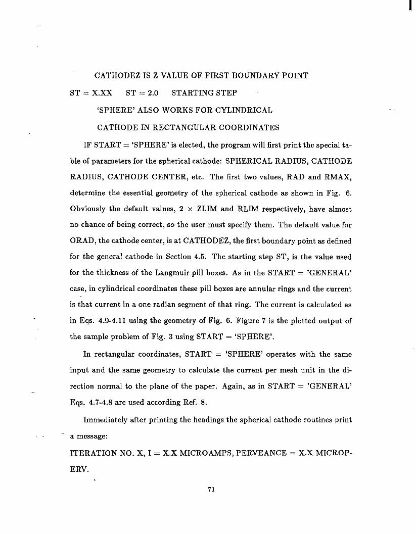
CATHODEZ IS Z VALUE OF FIRST BOUNDARY POINT

ST = X.Xx ST = 2.0 STARTING STEP ~~

‘SPHERE’ ALSO WORKS FOR CYLINDRICAL

CATHODE IN RECTANGULAR COORDINATES

IF START = ‘SPHERE’ is elected, the program will first print the special ta-

ble of parameters for the spherical cathode: SPHERICAL RADIUS, CATHODE

RADIUS, CATHODE CENTER, etc. The first two values, RAD and RMAX,

determine the essential geometry of the spherical cathode as shown in Fig. 6.

Obviously the default values, 2 x ZLIM and RLIM respectively, have almost

no chance of being correct, so the user must specify them. The default value for

ORAD, the cathode center, is at CATHODEZ, the first boundary point as defined

for the general cathode in Section 4.5. The starting step ST, is the value used

for the thickness of the Langmuir pill boxes. As in the START = ‘GENERAL’

case, in cylindrical coordinates these pill boxes are annular rings and the current

is that current in a one radian segment of that ring. The current is calculated as

in Eqs. 4.9-4.11 using the geometry of Fig. 6. Figure 7 is the plotted output of

the sample problem of Fig. 3 using START = ‘SPHERE’.

In rectangular coordinates, START = ‘SPHERE’ operates with the same

input and the same geometry to calculate the current per mesh unit in the di-

rection normal to the plane of the paper. Again, as in START = ‘GENERAL’

Eqs. 4.7-4.8 are used according Ref. 8.

Immediately after printing the headings the spherical cathode routines print

a message:

ITERATION NO. X, I = X.X MICROAMPS, PERVEANCE = X.X MICROP-

ERV.

71

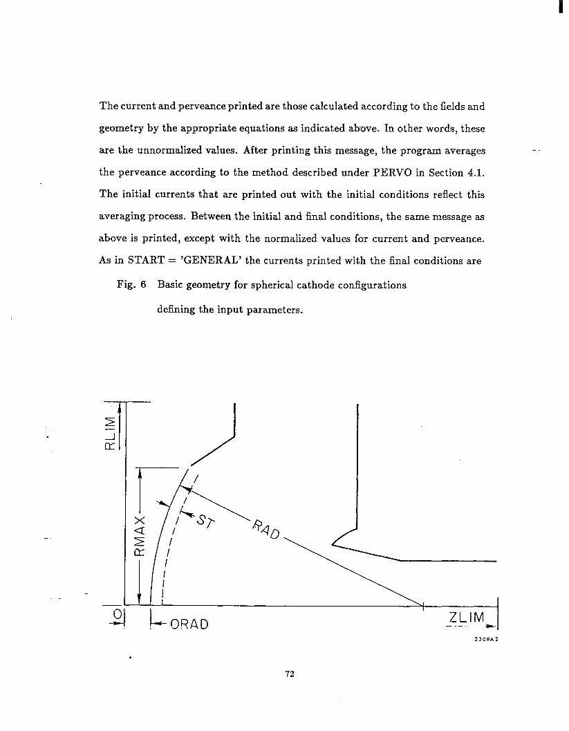
The current and perveance printed are those calculated according to the fields and

geometry by the appropriate equations as indicated ab-ove. In other words, these

are the unnormalized values. After printing this message, the program averages

the perveance according to the method described under PERVO in Section 4.1.

The initial currents that are printed out with the initial conditions reflect this

averaging process. Between the initial and final conditions, the same message as

above is printed, except with the normalized values for current and perveance.

As in START = ‘GENERAL’ the currents printed with the final conditions are

Fig. 6 Basic geometry for spherical cathode configurations

defining the input parameters.

2309A2

72

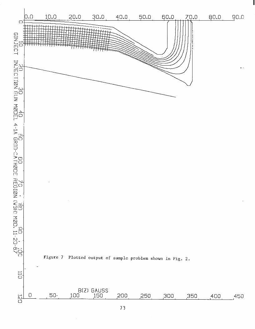
c

I-- J.

I

I-_ I

l- I

Figure 7 Plotted output of sample problem shown in F ig. 2.

B(Z) GAUSS 0 50* , ,100 ,150 ,200 ,250 ,300 ,350 ,400 450

73

divided by the initial radius (if in cylindrical coordinates), and thus give a mea-

sure of uniformity of cathode loading.

The special case of magnetic fields reaching the cathode, i.e., “immersed flow”

is treated by both SPHERE and GENERAL according to Busch’s theorem.12 The

program must use magnetic fields on the cathode and on the starting surface to

integrate the azimuthal motion through the gap between the cathode and the

starting surface. If there is any inconsistency in the off-axis magnetic fields within

f6 mesh units of the entire range of the starting area, then peculiar bunching

of the rays will occur. That is why the proper use of MAGORD and the careful

input of fields near the cathode were stressed in Section 4.4. Fortunately, any

problem of this sort becomes immediately obvious on examination of either the

starting conditions or the plots.

4.7 CARD STARTING

The program starting instructions are as follows:

START=‘CARDS’ START=‘GENERAL’ CARD STARTING

-.

zo=x.xx zo=o.o OLD ORIGIN IN NEW FRAME

HAVE UP TO MAXRAY DATA CARDS WITH (1 INTEGER, 8 FLOAT PT.)

NO., MASS, R, z, ENERGY (EV), ANGLE (RADIANS), CURRENT

(MICROAMPERES IN ONE RADIAN SEGMENT), TRANSVERSE ANGLE,

TRANSVERSE POSITION (PHI).

- FORMAT IS FREE FIELD FOR THE NEW C VERSION OF THE PROGRAM

CARDS STOP READING WITH RAY NO. GREATER THAN MAXRAY

IF RECTANGULAR COORDINATES:

74

PHI IS TRANSVERSE POSITION IN MESH UNITS.

CURRENT IS MICROAMPERES IN ONE MESH UNIT DEEP SEGMENT

SPECIAL TESTS IN RATNST; CROSSING OR 3-D SPACE CHARGE

IRAT=l IRAT=O 3-D SPACE CHARGE

IRAT= IRAT=O CROSSING DETECTION

USE OF NEGATIVE RAY NUMBERS:

IF IRAT=l (3-D SPACE CHARGE)

MAKE RAY NUMBERS NEGATIVE FOR BEAM EDGE CARDS.

USE BEAM EDGE CARDS (I=O) TO SIMULATE SPACE

CHARGE SPREADING OF A CYLINDRICAL BEAM OF

CURRENT I AND RADIUS R IN RECT. COORD.

PAIRS OF BEAM EDGE CARDS PRECEDE SETS OF RAY CARDS

DEFINING PART OF BEAM FOR WHICH 3-D SPACE CHARGE SPREAD-

ING IS TO BE SIMULATED. SEVERAL PARTS, DIFFERENTIATED BY

SELECTED ATTRIBUTES: E. G., ENERGY ALPHA OR RADIUS, CAN BE

USED SIMULTANEOUSLY WITH ANY NUMBER OF RAYS IN EACH PART.

END OF PART IS DEFINED BY NEXT RAY WITH NEGATIVE RAY NUM-

BER, WHICH BEGINS THE NEXT PART. -.

TO SIMULATE CYLINDRICAL BEAM SPACE CHARGE IN RECT. CO-

ORD. MAKE CURRENT PER MESH UNIT, I‘ = I/(PI * R) INSTEAD OF I‘

- = 2 * I/(PI * R) WHICH WOULD HAVE THE SAME CURRENT DENSITY.

IN OTHER WORDS, MAKE I‘(K) = I(K)/(2* R(K) INSTEAD OF I(K)/R(K).

NOTE THAT THIS REQUIRES TWICE AS MANY RAYS AS FOR CYLIN- .

75

DRICAL BEAM WITH SYMMETRY. BEAM EDGE CARDS (RAY < 0) AP-

PLY TO OFF-AXIS PENCIL IN CYL. COORD. ~~.

The START = ‘CARDS’ mode uses data cards for the initial conditions rather

than computing the initial conditions from a thermionic model. There are several

typical applications for this feature that will be described in some detail. There

are:

1. The simplest case of user specified data.

2. Use of cards generated by a preceding run to restart in a new segment of

the same problem.

3. Study thermal and other perturbing influences on a beam.

4. Rectangular coordinate application with a cylindrical beam, including cylin-

drical space charge and off axis bends.

User Specified Data

If START = ‘CARDS’ has been selected, the program will respond by printing

a table of appropriate parameters: STEP, NS, Z(O), SKAL, UNIT. Following the

end of the NAMELIST input &END card, the program will expect to read up

to MAXRAY cards with the starting data. A card with ray number greater

than MAXRAY will terminate this input. If MAXRAY cards are present, the

termination card should be used anyway. However, no effort should be made to

make MAXRAY agree with the number of cards used, so long as it is big enough.

The computer can, after all, count better than most humans.

Data to be entered on the ray cards consist of a ray number and the MASS,

followed by the initial values for R, Z, ENERGY, ANGLE, CURRENT, TRANS-

VERSE ANGLE and TRANSVERSE POSITION. The format is 15, F5,7F10.5. .

76

1. Ray Number: the ray number is only included for user convenience, and

for the termination purpose described above. Rays are numbered by the

program, sequentially as the cards are read in. Negative ray numbers have

special implications that will be described below.

2. MASS, 0 for electrons, N for the mass/charge ratio for ions. Note that this

is a new entry and although it can be safely omitted in the fixed format for

the FORTRAN program, in free field, the zeroes must be included.

3. R: the initial radial position in mesh units.

4. Z: the initial axial position in mesh units.

5. ENERGY (EV): Th e initial kinetic energy of the particle in electron volts.

It should be obvious, but sometimes requires stating, that ENERGY has

nothing whatever to do with the potential values on the boundaries, or on

the potential at which the ray tracing starts. For ray tracing, only fields

are important, not absolute potentials.

6. ANGLE: the initial angle that the ray makes with respect to the z-axis, in

radians.

7. CURRENT: the current in microamperes for a one radian segment of that

ray. In rectangular coordinates, it is for a one mesh unit deep segment.

8. TRANSVERSE ANGLE: the angle included between the ray and the R-Z

plane.

9. PHI: the initial transverse position. In rectangular symmetry, PHI is a

linear coordinate, measured in mesh units. In cylindrical symmetry, PHI is

the azimuthal position in radians.

77

Program Generated Cards

During the last program cycle, the program generates two sets of cards with

the initial and the final conditions of each ray according to the above format.

These cards may be punched, or saved as a data set in card format on a direct

access device. For the C program, these ‘cards’ are included right in the output

listing from which they can be readily extracted by a text editor. If it is planned

to use the cards in a subsequent run, it is only necessary to be sure they are

saved somehow. In a pinch, the same data are printed in the output and can be

hand punched.

Typically, these cards are intended to be used in a subsequent segment of a

problem. Thus the results of the sample problem, Fig. 3, are intended to be used

in the complete gun with card starting just past the grid. Between runs, it is

normal to expect that a different scale and origin will be used, otherwise there is

not. much reason for the second run. The companion parameters ZO and SKAL

are used to modify the data, as read in on the cards, as follows:

zo = x.xx zo = 0.0 OLD ORIGIN IN NEW FRAME

SKAL = X.Xx SKAL = 1.0 OLD MESH/NEW MESH

In words, if the first problem is plotted on the same graph with the second

problem, then the origin of the first problem will be found displaced left or right

by ZO mesh units in the new coordinate system. Usually ZO is negative. SKAL

is interpreted as the ratio of sizes of mesh units (in meters). Thus a problem

- in which many mesh units were used to calculate cathode conditions will have

a relatively smaller mesh than the follow on problem and SKAL < 1.0 in this

example. .

78

Thermal Effects

SUBROUTINE THERM IS CALLED IF THE PARAMETER TC > 0

TC=XXXX.X TC = 0 KELVIN TEMP. OF CATHODE

THREE MODELS ARE INCLUDED IN THIS VERSION

KRAY=2 KRAY=l TWO PART SPLIT, RANDOMIZED.

KRAY=S KRAY=l THREE RAY SPLIT

KRAY=5 KRAY=l FIVE RAY SPLIT

THREE RAY SPLIT PUTS CURRENTS IN 1-2-1 RATIO,

WITH 2 PARTS IN UNDEFLECTED RAY AND 1 PART

EACH IN RAYS WITH V(PERP)=SQRT(2KT/M), IN R-Z

PLANE, UP AND DOWN RELATIVE TO UNDEFLECTED RAY.

FIVE RAY SPLIT PUTS CURRENTS IN 1-5-8-5-1 RATIO

WITH V(PERP)=2*SQRT(2KT/M) FOR 1 PART RAYS

AND V(PERP)=l*SQRT(2KT/M) FOR 5 PART RAYS.

NO DEFLECTION FOR 8-PART CENTER RAY.

THERM CAN BE CALLED FOR START=‘SPHERE’, ‘GENERAL’, ‘CARDS’

OR ‘GENCARD’, NOT FOR START=‘CARDS’ WITH SAVE=2.

-. Rectangular Coordinates with Cylindrical Beams

The basic assumption in rectangular coordinates is that the beam consists of a

sheet extending infinitely in the directions in-and-out of the problem. The space

charge forces on such a beam are much greater than in cylindrical symmetry

because the field does not fall off by l/R. However, if the current is properly

reduced, the transverse space charge forces can be made the same as they would

79

be for a cylindrical beam. Further reductions in the current can compensate for

further expansion of the beam.

Consider first a uniform density cylindrical beam of total current I and radius

R. The current density is J = I/rR2. If one wished to have a rectangular

symmetry beam of thickness 2R at the same current density, the total current

per unit length would be

I’ = 2RJ = 21/7rR (equal densities) (4.14)

To define the rays in rectangular coordinates, one can divide I’ by some integer

n and make n rays, suitably spaced, each with a current of F/n. If one wishes

to use starting data from a previous run, then each ray has a current per unit

length I(K)/R(K). U n ess 1 the rectangular beam has reflection symmetry on the

z-axis, there would have to be twice as many trajectories created as in cylindrical

symmetry to represent both halves of the beam.

Consider now a particle of charge “e” on the edge of a cylindrical beam of

radius R and current I. The radial space charge force on the particle is

md2R/dt2 = eI/(27rRic,). (4.15)

The force on a similar particle next to an infinite current sheet in rectangular

coordinates is

md2Y/dt2 = eI’/(2ico).

To make d2R/dt2 = d2Y/dt2 we have only to require

(4.16)

80

I’ = I/rR (equal forces) .- (4.17)

This is just one half of the result for equal densities in (4.13). Thus, if the results

from the previous run were treated as described above, except divided by two,

then the initial space charge force on the rays would be the same as in cylindrical

coordinates.

A special feature allows the user to designate groups of rays, as few as one

per group, to be bounded by “beam edge” cards which do not carry current.

As the beam edge cards spread apart, the current on all rays within a group is

reduced proportionately. The groups may cross or overlap, but should not cross

their own beam edge rays. The initial conditions of the beam edge rays can be

chosen so that they do not cross the rays of the group. Beam edge cards are

designated by being inserted, with negative rays numbers, in pairs just before

the members of their group. Successive groups would thus be separated by the

pair of beam edge cards for the next group.

Beam edge cards may also be used in cylindrical coordinates. In this case,

the effect would be of an off-axis pencil beam, i.e., not an annular ring. Assuming

that the thickness of the pencil is small compared to the radial displacement, the

same factor of one-half should be applied to the initial currents as was derived

for rectangular coordinates.

IF IRAT= (R-Z AND PHI CROSSOVERS)

1) R-Z: MAKE RAY NUMBERS NEGATIVE FOR SEQUENTIAL RAYS

FOR WHICH FINAL CROSSOVER SHOULD BE DETECTED. CROSS-

INGS WILL BE LISTED AND PLOTTED. NEGATIVE RAY NUMBERS

81

SHOULD BE IN PAIRS. TO FIND CROSSOVERS WITH Z AXIS, RUN

A RAY WITH R=O,ALPHA=O PRECEDING THE RAY TO TEST AXIS

CROSSING.

2) PHI: LEAVE RAY NUMBERS POSITIVE FOR TRANSVERSE RAYS

TO DETECT LAST CROSSING OF PHI=PI* INTEGER.

A special application of beam edge cards is to specifically detect crossovers. For

this application, the beam edge control code is set to IRAT= in &INPUT5.

The program instruction comments appear above. This feature is used to find

the locus of foci to determine the position of the scintillator surface in image

intensifier tubes. No space charge is involved. Pairs of trajectories, started

sequentially from the same point with different initial conditions (energy and

direction) are focused to a crossing, which must be located exactly. The program

finds such crossovers and prints a table of their coordinates.

4-8 LAPLACE’S EQUATION APPLICATIONS

-.

START = ‘LAPLACE’ NO RAY TRACING

NS = X NS = 7 NUMBER OF LAPLACE CYCLES

LAPRH=l LAPRH=O USE LAPRH=l TO START READING

DATA CARDS WITH (R,Z SPACE CHARGE) FOR NON-ZERO POINTS.

END POINT INPUT BY R > RLIM.

Laplace’s equation has many applications besides solving electrostatic po-

tential problems. Some examples are temperature distributions and magnetic

- fields.

As a reminder, by Laplace’s equation one usually means V2r$ = 0, while

Poisson’s equation is V24 = p. The program always solves Poisson’s equation but .

82

with p = 0 on the first iteration. However, if one selects START = ‘LAPLACE’,

one can then add data cards with the coordinates (RjA), and the right hand or

space charge term for any non-zero point. These data are appended after the end

of the starting namelist and are terminated by R > RLIM. In the C program, a

new parameter LAPRH signals the program to begin reading the data cards for

the right hand side.

The program will then cycle for NS cycles on just these data, with no ray

tracing. It prints the potential map, or POTLIST, before and after the last cycle

to show how things may be changing. Following the last cycle, the program prints

a list of the fields, i.e., the derivatives of the potentials, on all the boundaries.

Fields at specified interior points can be obtained by making a dummy boundary

go through such points. Dummy boundary points have DELTAZ = 2.0 and can

be fitted according to the same rules as Neumann boundaries, i.e., along mesh

lines. The fields are normalized to 100% of the field on the first boundary point.

Choose it carefully, i.e., not where the field is near zero.

To do ray tracing with the solution found by LAPLACE, it is simply neces-

sary to set SAVE=1 in &INPUT5 of the first, LAPLACE, problem followed by

a second problem, without boundary data, but with ray tracing starting instruc-

tions. See the discussion under SAVE=1 in Section 4.1.

4.9 DIELECTRIC BOUNDARIES

The input provision for special boundary points, described in Section 3.2 can

be used for the particular case of a dielectric boundary. The difference equations

are only affected on the boundary of the dielectric. The normal method of using

this feature is to specify dummy boundary points, i.e., points with DELTAR =

83

DELTAZ = 2.0, which can be put in point-by-point or with the fitting (three-

point) method as lines.

The difference equations were derived by Seeger13 for the special cases of

horizontal and vertical dielectric boundaries. These relatively simple cases are

sufficient for most applications because the actual position and angle of even a

curved dieletric are relatively less important to the fields in the vicinity than the

fact that the boundary is located nearby. Thus a good approximation results from

a stepwise simulation of the dielectric and a small displacement to the nearest

mesh point does very little to the fields a few mesh units away.

- .

The coefficients of the difference equation are given by Eq. (3.3) and can be

expressed as:

LEFT = RIGHT = R (Vacuum)

UP = R + l/2

DOWN = R - l/2

(4.18)

For a horizontal dieletric, where ~1 is the dielectric constant for the lower region

and 6% is the constant for the upper region, the coefficients become:

LEFT = RIGHT = [E~(R - l/2) + E~(R + l/2)1/2 (Horizontal)

UP = e2(R + l/2)

DOWN = q(R - l/2)

(4.19)

For a vertical dielectric boundary, the coefficients become

84

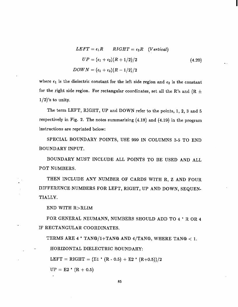
LEFT = qR RIGHT = ERR (Vertical)

UP = (~1 + EZ)(R + l/2)/2

DOWN = (cl + e2)(R - l/2)/2

(4.20)

where ~1 is the dielectric constant for the left side region and ~2 is the constant

for the right side region. For rectangular coordinates, set all the R’s and (R f

1/2)‘s to unity.

The term LEFT, RIGHT, UP and DOWN refer to the points, 1, 2, 3 and 5

respectively in Fig. 2. The notes summarizing (4.18) and (4.19) in the program

instructions are reprinted below:

SPECIAL BOUNDARY POINTS, USE 999 IN COLUMNS 3-5 TO END

BOUNDARY INPUT.

BOUNDARY MUST INCLUDE ALL POINTS TO BE USED AND ALL

POT NUMBERS.

THEN INCLUDE ANY NUMBER OF CARDS WITH R, Z AND FOUR

DIFFERENCE NUMBERS FOR LEFT, RIGHT, UP AND DOWN, SEQUEN-

TIALLY.

END WITH R>RLIM

FOR GENERAL NEUMANN, NUMBERS SHOULD ADD TO 4 * R OR 4 -.

IF RECTANGULAR COORDINATES.

TERMS ARE 4 * TAN@/l+TAN@ AND 4/TAN@, WHERE TAN@ < 1.

HORIZONTAL DIELECTRIC BOUNDARY:

LEFT = RIGHT = (El * (R - 0.5) + E2 * (R+0.5))/2

UP = E2 * (R + 0.5) .

85

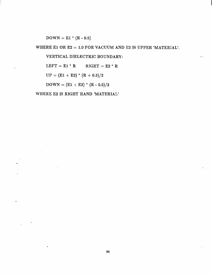
DOWN = El * (R - 0.5)

WHERE El OR E2 = 1.0 FOR VACUUM AND E2 IS UPPER ‘MATERIAL’.

VERTICAL DIELECTRIC BOUNDARY:

LEFT = El * R RIGHT = E2 * R

UP = (El + E2) * (R + 0.5)/2

DOWN = (El + E2) * (R - 0.5)/2

WHERE E2 IS RIGHT HAND ‘MATERIAL’

86

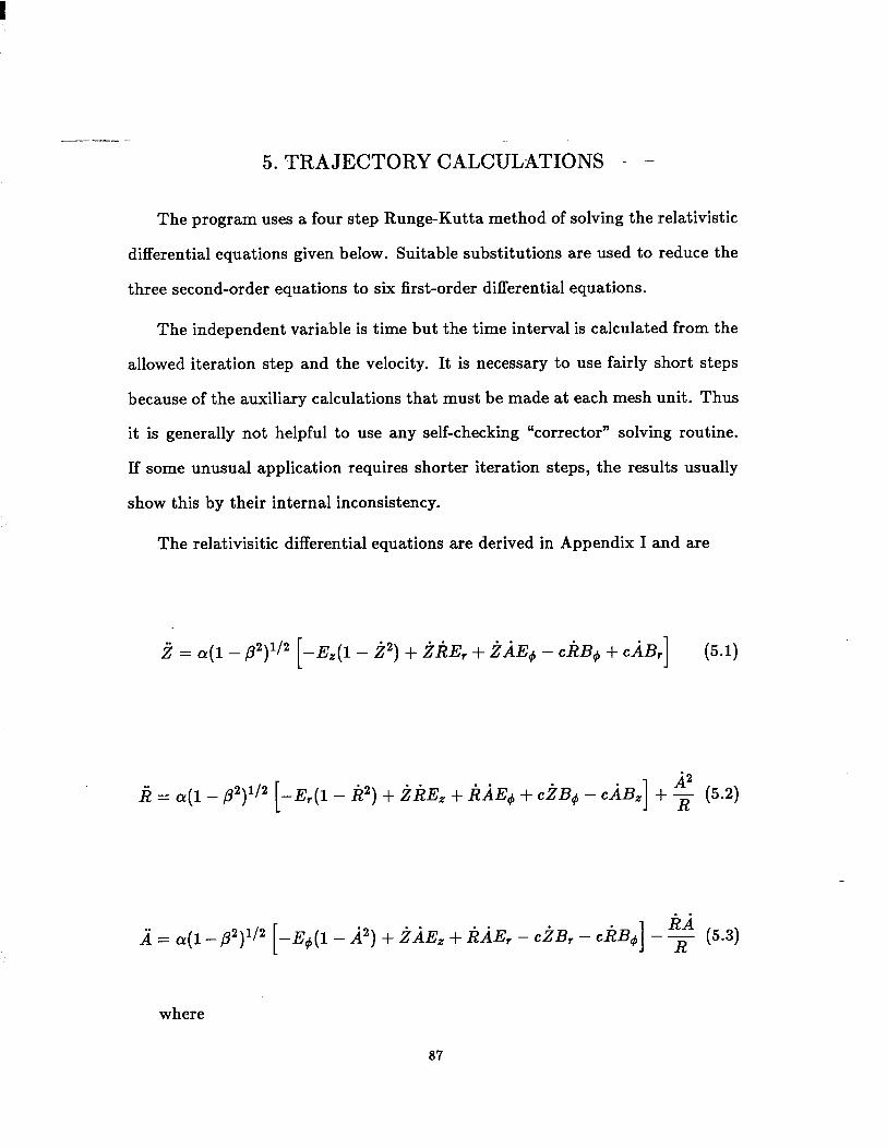
5. TRAJECTORY CALCULATIONS - -

The program uses a four step Runge-Kutta method of solving the relativistic

differential equations given below. Suitable substitutions are used to reduce the

three second-order equations to six first-order differential equations.

The independent variable is time but the time interval is calculated from the

allowed iteration step and the velocity. It is necessary to use fairly short steps

because of the auxiliary calculations that must be made at each mesh unit. Thus

it is generally not helpful to use any self-checking “corrector” solving routine.

If some unusual application requires shorter iteration steps, the results usually

show this by their internal inconsistency.

The relativisitic differential equations are derived in Appendix I and are

2 = a(1 - ,@)li2 [-E,(l - i”) + i&r + i@, - cliB# + CAB,] (54

A2 ii = a(1 - p2)li2 [-&(1 - h2) + ii& + hi& + c,kB4 - ciB,] + R (5.2)

A = d1 - P2)1’2 [-E#(l - A”) + i&, + &&, - &B, _ &$] -g (5.3)

where

87

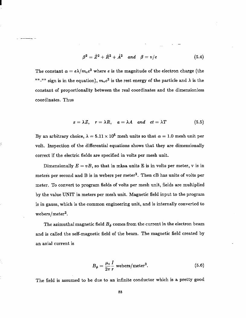
p2 = i2 + h2 -I- A2 and p = v/c (5.4

The constant a! = eX/m,c2 where e is the magnitude of the electron charge (the

“‘‘-“” sign is in the equation), moc2 is the rest energy of the particle and X is the

constant of proportionality between the real coordinates and the dimensionless

coordinates. Thus

2 = AZ, ?-=A& a= XA and et = XT P-5)

By an arbitrary choice, X = 5.11 x lo5 mesh units so that cx = 1.0 mesh unit per

volt. Inspection of the differential equations shows that they are dimensionally

correct if the electric fields are specified in volts per mesh unit.

Dimensionally E = vB, so that in mksa units E is in volts per meter, v is in

meters per second and B is in webers per meter2. Then cB has units of volts per

meter. To convert to program fields of volts per mesh unit, fields are multiplied

by the value UNIT in meters per mesh unit. Magnetic field input to the program

is in gauss, which is the common engineering unit, and is internally converted to

webers/meter2.

The azimuthal magnetic field B4 comes from the current in the electron beam

and is called the self-magnetic field of the beam. The magnetic field created by

an axial current is

PO I B$ = Gr webers/meter2. (5.6)

The field is assumed to be due to an infinite conductor which is a pretty good

88

approximation in the area in which the field is significant. After multiplying B+

by the scale factor and expressing r in meters which requires multiplying r by

the scale factor also, the scale factor cancels as might be expected. Thus the

scale factor only enters for external magnetic fields. The current I in (4.19) is the

summation of the current in the trajectories at lower radii than the trajectory

being calculated, but including the one being calculated.

Two field components are neglected. The azimuthal electric field is neglected

because of the axial symmetry assumed. The axial magnetic field can have a

contribution from the beam due to azimuthal velocity of the beam. The magni-

tude has been shown to be less than one gauss in most practical cases and so is

neglected.

The space charge is calculated to supply the right side of Poisson’s equation

which is

vq7 = E = .L 60 veo

(5.7)

The element of area for J is r x 1.0 square mesh units where r is the particle

radius. The velocity is only the Z-component since the space charge is being

spread between adjacent points on the same column. The one mesh unit space

between adjacent points accounts for the 1.0 in the area expression above.

In the finite difference form, (3.3) replaces (5.7), and the right hand side

becomes

RO = 36~ x lOgI x 1O-6 ABS(ZDOT) x 3 x 10s =

(3.77 x 10-4)1(K) ABS(ZDOT) (5.8)

89

-- -

where RO is to be spread between two points in inverse ratio to the distance

the ray is between them, I(K) is the current in the one radian segment of the

ray (in microamperes) and ZDOT is the velocity in units of c. If the angle of

inclination, dR/dZ, exceeds 45’, the calculation is made for RDOT. The absolute

value of ZDOT is used to allow a negative ZDOT. The explicit value of R in (3.3)

is canceled by the R which would convert the current to current density, thus

avoided special problems as R + 0.

In practice, however, there are still some space charge problems near the

axis. In rectangular coordinates, if the axis is a plane of symmetry, then any

trajectory between R = 0 and R = 1 has a mirror image between R=O and R=-1.

(A reminder again...when in rectangular coordinates, the axis still retain their

cylindrical labels.) To account for all the space charge on the axis, the calculated

charge is doubled. In cylindrical coordinates, the algorithm for distributing the

space-charge proportionately to the distance between the adjacent points is not

a very accurate solution. Good smooth laminar flow near the axis results by

simply making the space charge on the axis equal to that found for the first row.

90

~ I _ ~ .

6 . T R A J E C T O R Y A N A L Y S IS ._ - -

E G U N d o e s s o m e a n a l y s i s o f th e q u a l i ty o f th e b e a m to fi n d th e e m i tta n c e o f

th e e n s e m b l e o f p a rti c l e s . F o r th o s e n o t fa m i l i a r w i th th e c o n c e p t o f e m i tta n c e ,

d i s c u s s i o n s c a n b e fo u n d i n a n y b o o k a b o u t a c c e l e ra to r d e s i g n , s u c h a s th a t b y

S te ffa n .” R e c e n t v e rs i o n s o f th e p ro g ra m , i n c l u d i n g E G N 8 7 c , u s e th e c o m m o n

d e fi n i ti o n o f e m i tta n c e ;1 8

E = 4 x [ < x 2 > < x l 2 > - < x x x ’ > 2 ]1 /2

w h e re th e < > re p re s e n t a v e ra g e s a n d th e X a n d X ’ te rm s a re th e w e i g h te d s u m s ,

a n d s u m s o f s q u a re s , o f th e o rth o g o n a l q u a n ti ti e s x o r y . B e c a u s e th e p ro g ra m

i s u s i n g p a n d p ’, i n c y l i n d ri c a l c o o rd i n a te s , th e x a n d y te rm s a re fo u n d fro m

x = p c o s 4 , a n d s i m i l a r e x p re s s i o n s , w h e re 4 i s th e n e t a z i m u th a l a n g l e . In s te a d

o f s ta rti n g m a n y p a rti c l e s a t ra n d o m i n i ti a l v a l u e s o f 4 , i t i s s u ffi c i e n t to n o te

th a t e a c h b ra c k e t a b o v e c o n ta i n s a c o s 2 4 , w h i c h a v e ra g e s to 0 .5 . T h e s e h a l v e s a re

fa c to re d o u t o f th e s q u a re ro o t a n d c h a n g e th e c o e ffi c i e n t fo u r to a tw o . T h e fo u r

i s th e re to s i m u l a te a s q u a re d d i s tri b u ti o n , a s i n a u n i fo rm b e a m , a s c o m p a re d

to a n rm s d i s tri b u ti o n . T h e u n i ts o f e m i tta n c e a re m i l l i m e te r-m i l l i ra d i a n s , w h i c h

u s e s th e s c a l e fa c to r th a t i s d e fi n e d fo r th e p ro b l e m . E m i tta n c e c a l c u l a ti o n s a re

d e fi n e d a s th e a re a o f a n e l l i p s e , w h i c h i n v o l v e s a fa c to r o f 7 ~ w h i c h , b y c o n v e n ti o n

a n d to a v o i d c o n fu s i o n , i s s ta te d e x p l i c i tl y i n th e o u tp u t u n i ts , a n d i s th e re fo re

o m i tte d fro m th e a b o v e e x p re s s i o n .

E x p e ri e n c e h a s s h o w n th a t th e e m i tta n c e v a l u e s c a l c u l a te d i n th i s w a y a re i n

re a s o n a b l e a g re e m e n t w i th w h a t s h o u l d b e e x p e c te d fro m w e l l d e s i g n e d e l e c tro n

g u n s . T h e re s u l ts a l s o a g re e re a s o n a b l y w i th p ro g ra m s th a t a re m o re s ta ti s ti c a l i n

9 1

concept. If it is planned to compare emittance numbers, the user should endeavor

to have a reasonably large number of trajectories, that is, perhaps at least thirty,

so as to have some statistical validity.

The emittance calculation also gives a value for the “invariant” or “normal-

ized” emittance which is given by;

where p = V/C and 7 = (1 - p2)-li2. Th’ q 1s uantity has the property that it is

invariant to further acceleration. That is, of course, provided the acceleration and

transport of the beam are not accompanied by aberrations that further degrade

the quality of the beam. The momentum used to find the product ,87 is that of

the first trajectory.

At the end of each run, after the last set of trajectory plots have been gener-

ated, two extra plots are created;

1. One is of the final current density as a function of final beam radius. This is

a rather crude profile of a histogram of currents found in ten bins between

p = 0 and the largest value of p. It is normalized to 1.0 at the peak

intensity. The result is frequently a sort of Rocky Mountain profile which

still resembles the actual current distribution to some degree.

2. The second plot is of final p’ = dp/dz us. p. This is essentially a plot of

phase space from which the emittance, as discussed above, can be under-

stood. A very good beam, with low emittance and no aberrations, would

have all the points plotted in this way, lie in a straight line. Most electron

guns, particularly if there is significant area convergence between the area

92

of the cathode and that of the beam, will exhibit some spherical aberra-

tion, in which the rays from the outer part of the beam cross over the inner

ones. The EGUN program invariably shows at least some such aberration

at the outer edge of any gun. This may be due to the way space charge is

allocated near the edge, or it may be real, or some of both.

There is one more plot available, for azimuthal motion. If the parameter

IPHI has been set to one of the ray numbers, a single curve will be plotted of the

azimuthal position us. Z. This is either the angle PHI, or the position PHI if in

rectangular coordinates. The plot is made for the ray designated by IPHI.

The current density profile, which was described above, should not be con-

fused with the emission current density which can be found by examining the

values for I(K)/R that are printed with the final conditions of each cycle. The

initial set of currents are the I(K) va ues 1 that are actually used by the program,

and are the currents (microamperes) in a one radian segment of the ring of charge.

Since current does not change during transport, the final data would be the same

as the initial current, thus wasting space in the output. Instead, the final num-

bers are the initial currents divided by the initial radius, to give values that are

proportional to initial current density, for example at a cathode, and can be used

to diagnose cathode emission uniformity.

To emphasize the importance of uniform emission density, and also to close

this section, it is appropriate to pass on one piece of “wisdom” gained from

simulating many electron guns. That is, to make a good electron gun, meaning

one with good beam quality, strive to get the space charge limited emission as

uniform as possible. The best guns are usually uniform to within 10% across the

face of the cathode.

93

REFERENCES - _ -

1. W. B. Herrmannsfeldt, Electron Trajectory Program, SLAC 226, Stanford

Linear Accelerator Center, Stanford, CA 94305, November 1979.

2. B. W. Kernighan and D. W. Ritchie, The C Programming Language, Pren-

tice Hall.

3. Metawindow is a registered trademark of the Metagraphics Software Cor-

poration, PO Box 66779, Scotts Valley, CA 95066.

4. Judith Colman, The Use of the IBM-PC Computer in Accelerator Design

Calculations, Proceedings of the 1986 Linear Accelerator Conference, Stan-

ford Linear Accelerator Center, Stanford, CA 94305, June 1986. Ms. Col-

man’s address is Neutral Beam Division, Brookhaven National Laboratory,

Upton, NY 11973.

5. Forsythe and Wasow, Finite Difference Methods for Partial Differential

Equations, Wiley and Sons.

6. Vladimir Hamza, NASA TN D-1323, TN D-1665, TN D-1711, Lewis Re-

search Center, Cleveland, Ohio, (1963).

7. C. Weber, Numerical Solution of Laplace’s and Poisson’s Equations and

the Calculation of Electron Trajectories and Electron Beams, Volume I,

Focusing of Charged Particles, A. Septier, Ed., Academic Press (1967).

8. Richard S. Varga, Matrix Iterative Analysis, Prentice Hall.

9. D. Bruce Montgomery,Solenoid Magnet Design, Wiley-Interscience, John

Wiley and Sons, New York (1969).

10. J. R. M. Vaughn, “Representation of Axisymmetric Magnetic Fields in

Computer Programs,n IEEE Trans. on Electron Devices, ED-19,No. 2,

94

--

Feb. 1972, pp. 144-152. _ - . .

11. K. R. Spangenburg,Vacuum Tubes,McGraw Hill, New York (1948).

12. K. R. Spangenburg,FundamentalsMElectronDevices,McGraw Hill, New

York (1957).

13. I. Langmuir and K. B. Blodgett, Phys. Rev. 22, 347 (1923).

14. G. R. Brewer, High Intesity Electron Guns, Focusing of Charged Particles,

Volume II, A. Septier, Ed., Academic Press (1967).

15. H. Busch, Ann. Physik 4,8& 974 (1926). See the above reference by Brewer

for a treatment of this subject.

16. J. A. Seeger, Proc. of IEEE, 56, 1393, (1968).

17. K. G. Steffen, High Energy Beam Optics,Interscience Monographs, John

Wiley and Sons, New York (1965).

18. P. M. Lapostolle, IEEE Trans l8, 1101, (1971).

95

APPENDIX I - ._ - - DERIVATION OF EQUATIONS OF MOTION

The equations of motion are derived from the relativistic Lorentz force equa-

tion

d(mv3= dt -e(Jl?+v’xd), (1)

where e is the magnitude of the charge of an electron. The electron velocity

vector V, expressed in cylindrical coordinates is

v’ = u,i + u,+ + u&. (2)

Here uZ, ur and u4 are unit vectors and 2G = r$ is the azimuthal or peripheral

velocity. The left side of Eq. (1) can be found from

where me is the electron rest mass. Differentiating Eq. (3) yields

where

!LL = uz2 + ur(r” - nj2) + u&+6 + 4)

(3)

which becomes

96

_ - . .

$; = u,; + ur(Y - b2/r) + u&i/r + ii).

From

2) = (i2 + f2 + iL2p2

where v is the scalar velocity, we have

dv - = +ii + ii: + q. dt v

(6)

(7)

@ I

Substituting Eqs. (6), (7) and (8) in Eq. (4) yields

!.k.$=m,(l-~)~3’2[1 -p + ir” + q (z&i + u,i + u&L) (9)

+{1-~}{u,i+..(i-ir2/r)+u~(i++a)}].

Equation (9) can be expanded and grouped by vector components yielding

C@$=m0(1-$)-3’2[uz{ &+ci)+i(l-g+;)}

+ ur { $i(BI+&) - - l- 2 +r T ( “‘) -(l-g+!T)} (10)

+ 214 $i(Z + ir”) + y 1

-* (1-g) +z(1-$+$)}I.

A similar vector component expansion can be made for the right side of Eq. (1)

yielding

97

db-4 - = -e dt uz(Ez + iB# - id,) + u,(E, + id, - 234) + u#(Ed + iB, - iB,) 1 .

(11) Equating vector components we have finally

mO (l- $)m3’2 { ( v2 i2) ” l--p+cz z++~+giii } = -e(Ez++Bd-&B,),

mo(1-!!!)m3’2{$+~~+ ( v2 ia)” l-s+2 r++y iL2 ( 1 - (14

V2 - c2 >, (13)

= - e(E, - 334 + id?,),

and

- 2 - C2 )I (14

= - e(E4 + 23, - iB,).

For computer programming it is convenient to express the variables in a

normalized form. Accordingly, we let

2 = AZ, r = XR, a= XA and ct = XT. (15)

We differentiate with respect to 2’ = et/X to get

98

. - . .

c2z i=&, z= - A ’

1: = cl& c2ii r”=- x ’

and

From the definitions in Eqs. (16) it follows that

212 pLCZ=i2+@ffp.

(16)

(17)

Note that the time derivatives of the normalized displacements, Z, R and A, are

with respect to T=ct/X. Making the normalizing substitutions in Eqs. (12),

(lg), and (17) yields

mOc2 X(1 - /32)3/2

[(l - p2 + i2)Z + iitli2 + iAA]

1 =-- E,+ckB,p-CAB, , (18)

m0c2 X(1 - p2)W [

k2 ILki + (1- p2 + Itt2)ii + M;I - &l - pz) 1 (19)

=- e E,- C ciB++ckB, , 1 and

m0c2 . . . . X(1 - /32)3/2

AZZ+AI#+(1-/?2+A2);i+ 1 (20) =- e Eg+ciB,-c$!B, [ 1 .

Our goal is to get separated equations solved for the second order derivative

99

I

of each of the orthogonal variables. To solve the eqtiations,.we arrange them in

the form

A$‘+ B# + Cl;i = D1

A2.2 + Baii + C,A: = D2 (21)

A32 + B35 + C3k: = D3

and apply the standard determinant method of solving simultaneous equations.

Arranging Eqs. (US), (19) and (20) in the form of Eq. (21) yields

(I- p2 + i2)i + ihii + i/iii = -eX(l - p2)3/2(& + &B4 - &jr), m0c2 (22)

A2 Iii2 + (1 - p2 + IP)ii + hii = (1 - p2)F - -f&(1 - py

(23) x (E, - ciBd + CAB,),

and

. . . . . .

AZ2 + /i&ii + (1 - p2 + i2)i = -(l - p2)y - --$(l - p2)3’2 (24)

x (E+ + ciB, - cIiB,).

The determinant of the coefficients is

A =(I - p2 + i2) [(I -p2 + $)(I -p2 + ~2) -/$d2]

+ ili piA2 - ik(l - p2 + ““)I

+ ik [i&i - Ai(1 - p2 + ““,I

=(l - p2 + i2)(1 - P2)(1- p2 + fp + $)

- .&-?(l - p2) - &$(l - py

=(l - py(l- p2 + 22 + $ + AZ)

100

which is simply _ - .

A = (1 - /?2)2. (25)

It is convenient to let cx = eA/moc 2. The axial acceleration 2, is given by

Ag = D1(B2C3 - C2B3) + D2(C1B3 - B1C3) + D3(B1C2 - C1B2)

which becomes

(1 - p”)“2 =[-a(1 - /32)3/2(Ez + ckB4 - CAB,)]

x [(l - p2 + 2)(1 - p2 + 2) - Iw]

A2 + [(l - pa)% - a(1 - /?2)3/2(Er - ciB4 + CAB,)]

x [hiA - iiql - p2 + AZ)] . .

+ [-(1 - p2,y - a(1 - /32)3/2(E4 + ciB, - &B,)]

x [ili2A - (1 - p2 + S)iA] .

Simplified, the above equation yields

.f =a(1 - ,O”)‘/“[-(Ez + cliB# - eiB,)(l - p2 + Ii2 + /i2)

+ (E, - ciB$ + ciB,)iIi + (IQ, + ciB, - diB,)ii].

Noting that (1 - p2 + k2 + A2) = 1 - i2, we have finally

.if = a(1 - p2)1/2[-&(1 - i2) + iEiE, + iiE, - c&B4 + CAB,] . (26) -

The radial acceleration k, is given by

Ai = D&W2 - A2C3) + Dz(A&3 - A3C1) + D3(A2C1 - A1C2)

101

which becomes _ - . .

(1 - p2)2iz =[-a(1 - p2)3/2(Ez + clfLBO - CAB,)]

x [Ii&i2 -lii(l-p2+A2)]

k2 + [(I - P2)x - ~(1 - p2)3/2(Er - ciB4 + CAB,)]

x [(l - p2 +9)(1-p + A") - 921 (27)

. .

+[-(l-&y - a(1 - p2)3’2(E4 + ciB, - cliB,)]

x [i21Li -kA(1-p2+i2)].

Simplified, the above equation yields

ii = a(1 - /3')'/'[ (E, + ciB# - CAB,) ii

- ( E, - ciB+ + CAB, )(l-P2+ia+2)

+ (E4 + ciB, - &B,) &A]

A2 +R(1-p2+i2+A2)+~.

Noting that (1 - p2 + .k2 + A’) = (1 - k2), we have finally

A2 ii = a(1 - P2)1/2[-Er(l - li2) + iIiE, + lbiE$ + ciB# - CAB,] + --. (28)

The azimuthal acceleration 2, is given by

A;l. = Dl(AzB3 - AsB2) + D2(A& - AIBB) + D3(A1B2 - A2Bl)

102

I

which becomes _ - . .

(l- p2)2;1 =[-cx(l- p2)3/2(Ez + chBg - c/iB,)][hi2i - ii(l- p2 + h2)] A2

+ Kl - P2)jj- - cr(l- /32)3/2(Er - ciBd + CAB,)]

x [ki2d-A~(l-p2+i2)] . .

+ [(l - pz)Jg - a(1 - p2)"/"(E4 + ciB, - &B,)]

x [(l- p2 + 9)(1- p2 + I?) - i2Ei2].

Simplified, the above equation yields

A=a(l-p) [( 2 1'2 E,+chB4-ciB,)ii+(E,-eiBm+ ciB,)&

E4+ciB,-eliB, ) (l-82 +i2 +I?)]

- !g (I_ p2 + i2 + fi2) A,“.

Noting that (1 - p2 + ,k2 + k2) = (1 - A2) we have finally

2=a(l-~2)1'2[-E&-i2)+~AE,+~~E,-c~B,+cBB,] -g. (29)

103

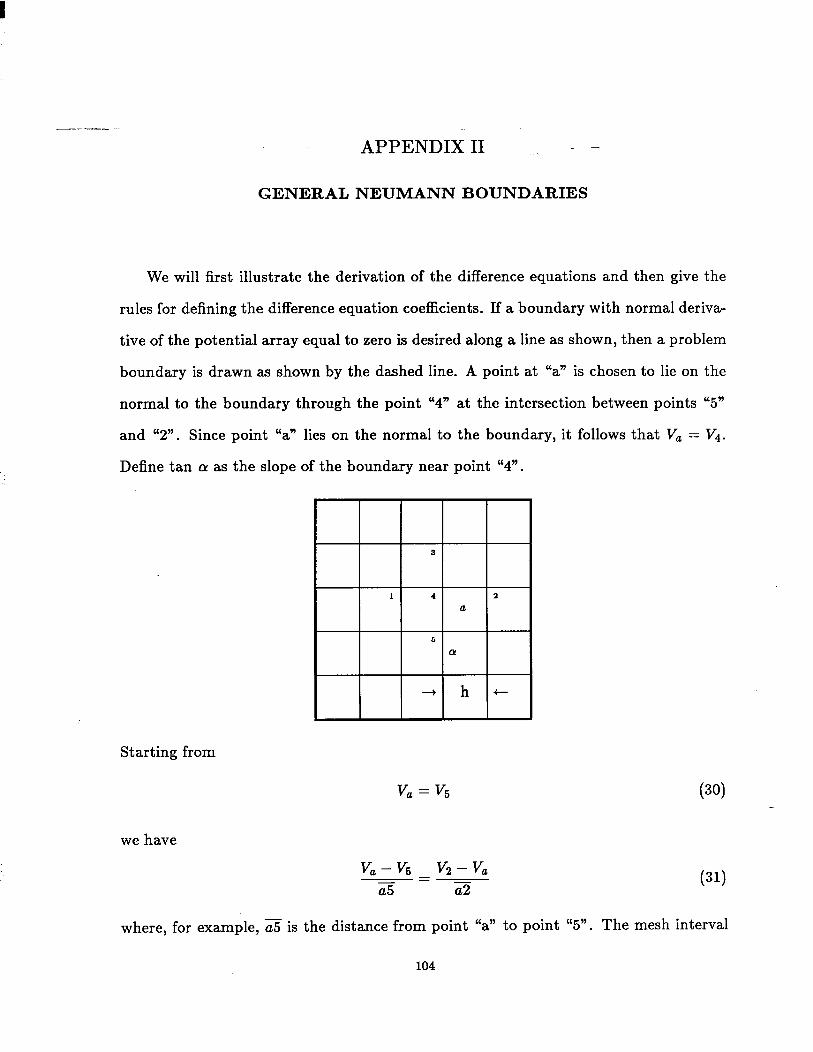
APPENDIX II ._ - -

GENERAL NEUMANN BOUNDARIES

We will first illustrate the derivation of the difference equations and then give the

rules for defining the difference equation coefficients. If a boundary with normal deriva-

tive of the potential array equal to zero is desired along a line as shown, then a problem

boundary is drawn as shown by the dashed line. A point at “a” is chosen to lie on the

normal to the boundary through the point “4” at the intersection between points “5”

and “2”. Since point “a” lies on the normal to the boundary, it follows that V, = Vi.

Define tan CI! as the slope of the boundary near point “4”.

Starting from

v, = v5 (30)

we have

va - v5 v2 - va = a5 a2 (31) -.

where, for example, a5 is the distance from point “a” to point “5”. The mesh interval

104

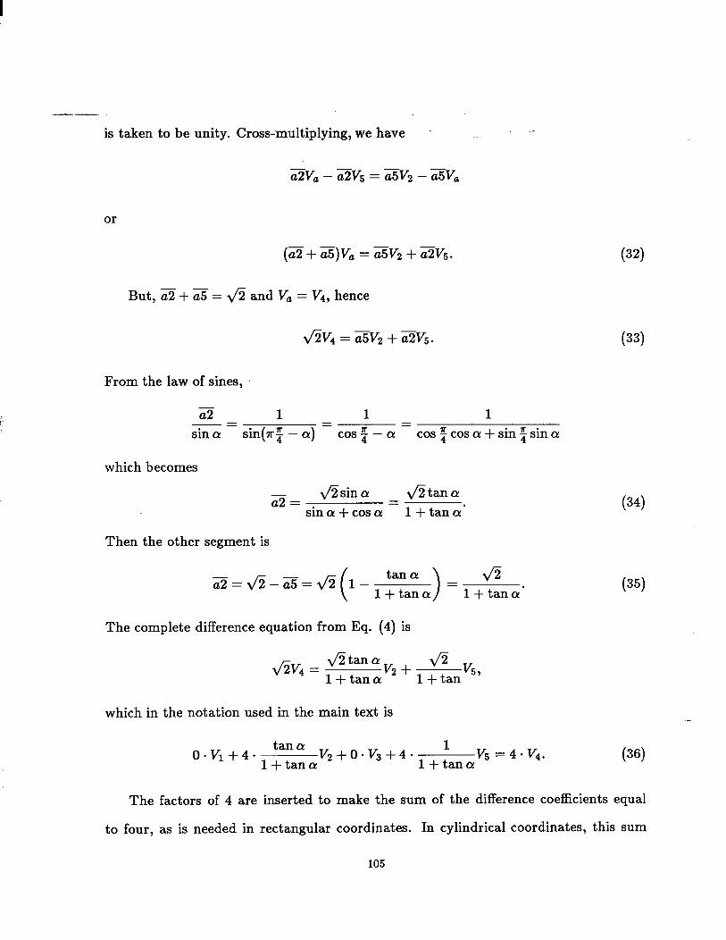
is taken to be unity. Cross-multiplying, we have - ~~_ -

- - a2V, - a2V5 = a5V2 - XV,

or

(ia+iiqV, =z& +a2V5.

-- But, a2 + a5 = fi and V, = Vi, hence

l/s4 = a5V2 + a2V5.

From the law of sines,

a2 1 1 1 - = = = sin (Y sin(7r: - CX) cos 2 - a cos%cosa!+sin~sina

which becomes

- 6 2sina fit ana! a2 =

sina+coscr! = l+tancr’

Then the other segment is

- a2454545 l- tana ( 1

fi = l+tana! l+tancr’

The complete difference equation from Eq. (4) is

&v4 = JZtanav2+ a l+tancr l+tan

v5,

which in the notation used in the main text is

tan LY: 1 0.v1+4-

l+tana! v2+o’v3+4*

l+tana! v5 =4-F/4.

(32)

(33)

(34

(35)

(36)

The factors of 4 are inserted to make the sum of the difference coefficients equal

to four, as is needed in rectangular coordinates. In cylindrical coordinates, this sum

105

should be 4 - R. Note that the derivation presented-above was for the slope, tan Q <l.

For a negative slope, the similar derivation uses Vi and Vs, with the same values of

slope. That is, use only positive values of tan Q that are less than 1.0. If the slope is

greater than 1.0, the two coefficients are interchanged, so that the larger term, l/(1 +

tan CY), goes with the point nearest to the normal to the boundary.

For CY = 45’, the difference terms both equal 2.0, which are exactly the terms

generated if both DELTAR and DELTAZ are 0.0, that is, the conditions for a double

Neumann boundary are in fact the conditions for a 45’ Neumann boundary. In many

applications it is possible to use a 45’ Neumann boundary and avoid the complications

of this section.

Note that in application, the points used for general Neumann points must have been

defined as Neumann boundary points during the boundary input process. The internally

generated difference coefficients are then over written by the method supplied to input

special boundary coefficients at the end of the regular boundary input, by signalling

with a 999 entry on the last input card.

106

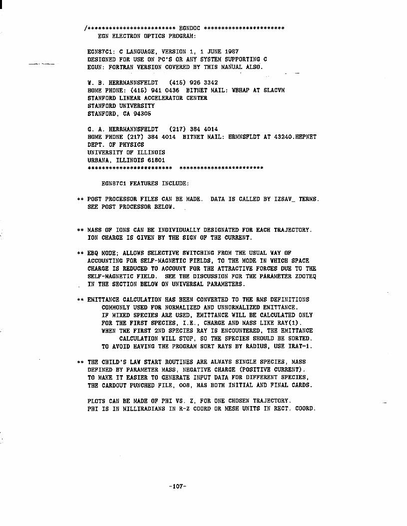
/************************** EGNDOC *********************** EGN ELECTRON OPTICS PROGRAM:

EGN87Cl: C LANGUAGE, VERSION I, I JUNE 1987 DESIGNED FOR USE ON PC'S OR ANY SYSTEM SUPPORTING C EGUN: FORTRAN VERSION COVERED BY THIS MANUAL ALSO.

_ - . . W. B. HERRMANNSPELDT (415) 926 3342 HOME PHONE: (415) 941 0436 BITNET MAIL: WBHAP AT SLACVM STANFORD LINEAR ACCELERATOR CENTER STANFORD UNIVERSITY STANFORD, CA 94305

G. A. HERRMANNSFELDT (217) 384 4014 HOME PHONE (217) 384 4014 BITNET MAIL: HRMNSFLDT AT 43240.HEPNET DEPT. OF PHYSICS UNIVERSITY OF ILLINOIS URBANA, ILLINOIS 61801 ******Fe***************** ************************

EGN87Cl FEATURES INCLUDE:

** POST PROCESSOR FILES CAN BE MADE. DATA IS CALLED BY IZSAV- TERMS. SEE POST PROCESSOR BELOW.

** MASS OF IONS CAN BE INDIVIDUALLY DESIGNATED FOR EACH TRAJECTORY. ION CHARGE IS GIVEN BY THE SIGN OF THE CURRENT.

** EBQ MODE; ALLOWS SELECTIVE SWITCHING FROM THE USUAL WAY OF ACCOUNTING FOR SELF-MAGNETIC FIELDS, TO THE MODE IN WHICH SPACE CHARGE IS REDUCED TO ACCOUNT FOR THE ATTRACTIVE FORCES DUE TO THE SELF-MAGNETIC FIELD. SEE THE DISCUSSION FOR THE PARAMETER ZDOTEQ IN THE SECTION BELOW ON UNIVERSAL PARAMETERS.

** EMITTANCE CALCULATION HAS BEEN CONVERTED TO THE RMS DEFINITIONS COMMONLY USED FOR NORMALIZED AND UNNORMALIZED EMITTANCE. IF MIXED SPECIES ARE USED, EMITTANCE WILL BE CALCULATED ONLY FOR THE FIRST SPECIES, I.E., CHARGE AND MASS LINE RAY(l). WHEN THE FIRST 2ND SPECIES RAY IS ENCOUNTERED, THE EMITTANCE

CALCULATION WILL STOP, SO THE SPECIES SHOULD BE SORTED. TO AVOID HAVING THE PROGRAM SORT RAYS BY RADIUS, USE IRAT=I.

** THE CHILD'S LAW START ROUTINES ARE ALWAYS SINGLE SPECIES, MASS DEFINED BY PARAMETER MASS, NEGATIVE CHARGE (POSITIVE CURRENT). TO MANE IT EASIER TO GENERATE INPUT DATA FOR DIFFERENT SPECIES, THE CARDOUT PUNCHED FILE, 008, HAS BOTH INITIAL AND FINAL CARDS.

PLOTS CAN BE MADE OF PHI VS. Z, FOR ONE CHOSEN TRAJECTORY. PHI IS IN MILLIRADIANS IN R-Z COORD OR MESH UNITS IN RECT. COORD.

-107-

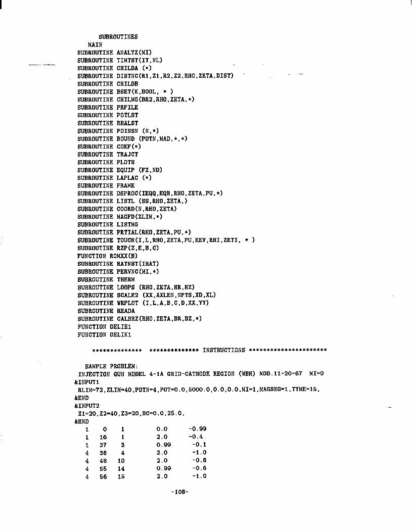
SUBROUTINES MAIN

SUBROUTINE ANALYZ(M1) SUBROUTINE TIMTST(IT,NL) SUBROUTINE CHILDA (*) SUBROUTINE DISTNC(Rl,Zl,R2,Z2,RHO,ZETA,DIST) - . . - - SUBROUTINE CHILDB SUBROUTINE BSET(K,BOOL, * ) SUBROUTINE CHILMG(BR2,RHO,ZETA,*) SUBROUTINE PRFILE SUBROUTINE POTLST SUBROUTINE RHALST SUBROUTINE POISSN (N,*) SUBROUTINE BOUND (POTN,MAD,*,*) SUBROUTINE COEF(*) SUBROUTINE TRAJCT SUBROUTINE PLOTS SUBROUTINE EQUIP (FZ,ND) SUBROUTINE LAPLAC (*) SUBROUTINE FRAME SUBROUTINE DSPROC(IEQQ,EQB,RHO,ZETA,PU,*) SUBROUTINE LISTL (ss,RHO,ZETA,) SUBROUTINE COORD(N,RHO,ZETA) SUBROUTINE MAGFD(ZLIM,*) SUBROUTINE LISTMG SUBROUTINE PRTIAL(RHO.ZETA,PU,*) SUBROUTINE TOUCH(I,L,RHO,ZETA,PU,EEV,RHI,ZETI, * ) SUBROUTINE RZP(Z,E,B,C) FUNCTION ROMXX(B) SUBROUTINE RATNST(IRAT) SUBROUTINE PERVNC(MI,*) SUBROUTINE THERM SUBROUTINE LOOPS (RHO,ZETA,HR,HZ) SUBROUTINE SCALE2 (XX,AXLEN,NPTS,XD,XL) SUBROUTINE WRPLOT (I,L,A,B,c,D,xX,YY) SUBROUTINE READA SUBROUTINE CALBRZ(RHO,ZETA,BR,BZ,*) FUNCTION DELIEI FUNCTION DELIKI

************** **********e*** INSTRUCTIONS **********************

SAMPLE PROBLEM: INJECTION GUN MODEL 4-1A GRID-CATHODE REGION (WBH) MOD.I~-20-67 MI=O

&INPUT1 RLIM=72,ZLIM=40,POTN=4,POT=O.O,5OOO.O,O.O,O.O,MI=l,~GSEG=l,TYME=l5,

&END &INPUT2

Zl=20,Z2=40,Z3=20,BC=O.O,25.0, &END

IO 1 0.0 -0.99 I 16 I 2.0 -0.4 I 37 3 0.99 -0.1 4 38 4 2.0 -1.0 4 48 10 2.0 -0.8 4 55 14 0.99 -0.6 4 56 15 2.0 -1.0

-108-

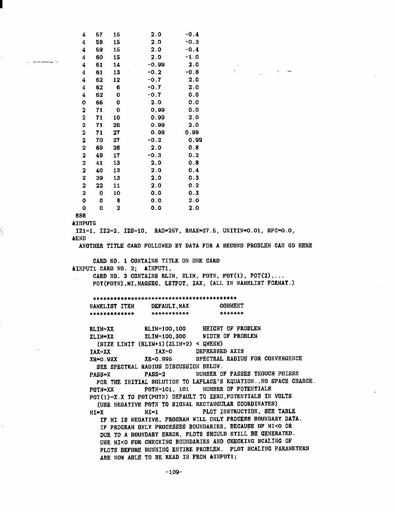
4 4 4 4 4 4 4 4 4 0 2 2 2 2 2 2 2 2 2 2 2 2 0 0

888 &INPUT5

57 15 2.0 -0.4 58 15 2.0 -0.3 59 15 2.0 -0.4 60 15 2.0 -1.0 61 14 -0.99 2.0 61 13 -0.2 -0.8 62 12 -0.7 2.0 62 6 -0.7 2.0 62 0 -0.7 0.0 66 0 2.0 0.0 71 0 0.99 0.0 71 IO 0.99 2.0 71 26 0.99 2.0 71 27 0.99 0.99 70 27 -0.2 0.99 69 26 2.0 0.8 49 17 -0.3 0.2 41 13 2.0 0.8 40 13 2.0 0.4 39 13 2.0 0.3 22 II 2.0 0.2

0 IO 0.0 0.3 0 8 0.0 2.0 0 2 0.0 2.0

IZI-I, IZ2=2, IZS=IO, RAD=257, RMAX=37.5, UNITIN=O.OI, SPC=O.O, &END

ANOTHER TITLE CARD FOLLOWED BY DATA FOR A SECOND PROBLEM CAN GO HERE

CARD NO. I CONTAINS TITLE ON ONE CARD &INPUT1 CARD NO. 2; &INPUTI,

CARD NO. 3 CONTAINS RLIM, ZLIM, POTN, POT(l), POT(2),... POT(POTN).MI,MAGSEG, LSTPOT. IAX, (ALL IN NAMELIST FORMAT.)

****************************************** NAMELIST ITEM DEFAULT.MAX COMMENT ************* *********** *******

RLIM=XX RLIM=100,100 HEIGHT OF PROBLEM ZLIM-XX ZLIM=100,300 WIDTH OF PROBLEM

(SIZE LIMIT (RLIM+I)(ZLIM+2) < QMESH) IAX-XX l-AX=0 DEPRESSED AXIS XR=O.SXX XR=0.995 SPECTRAL RADIUS FOR CONVERGENCE

SEE SPECTRAL RADIUS DISCUSSION BELOW. PASS=X PASS=2 NUMBER OF PASSES THOUGH POISSN

FOR THE INITIAL SOLUTION TO LAPLACE'S EQUATION..NO SPACE CHARGE. POTN=XX POTN=IOI, 101 NUMBER OF POTENTIALS POT(l)=X.X TO POT(POTN) DEFAULT TO ZERO,POTENTIALS IN VOLTS

(USE NEGATIVE POTN TO SIGNAL RECTANGULAR COORDINATES) MI=X MI=1 PLOT INSTRUCTION, SEE TABLE

IF MI IS NEGATIVE, PROGRAM WILL ONLY PROCESS BOUNDARY DATA. IF PROGRAM ONLY PROCESSES BOUNDARIES, BECAUSE OF MI<0 OR DUE TO A BOUNDARY ERROR, PLOTS SHOULD STILL BE GENERATED. USE MI<0 FOR CHECKING BOUNDARIES AND CHECKING SCALING OF PLOTS BEFORE RUNNING ENTIRE PROBLEM. PLOT SCALING PARAMETERS ARE NOW ABLE TO BE READ IN FROM BINPUTI;

-109-

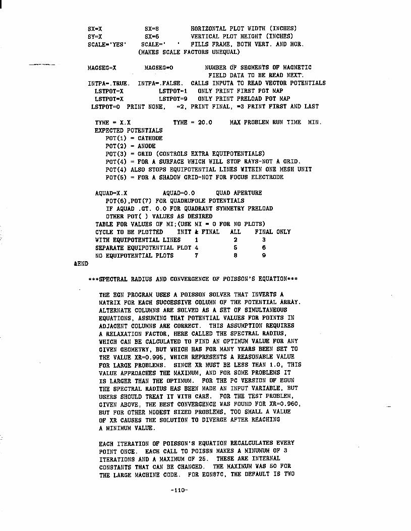
sx=x SX=8 HORIZONTAL PLOT WIDTH (INCHES) SY=X SX=6 VERTICAL PLOT HEIGHT (INCHES) SCALE='YES' SCALE=' ' FILLS FRAME, BOTH VERT. AND HOR.

(MAKES SCALE FACTORS UNEQUAL)

MAGSEG=X MAGSEG=O NUMBER OF SEGMENTS OF MAGNETIC FIELD DATA TO BE-READ NEXT-.

INTPA=.TRUE. INTPA=.FALSE. CALLS INPUTA TO READ VECTOR POTENTIALS LSTPOT=X LSTPOT=l ONLY PRINT FIRST POT MAP LSTPOT=X LSTPOT=O ONLY PRINT PRELOAD POT MAP

LSTPOT=O PRINT NONE, =2, PRINT FINAL, =3 PRINT FIRST AND LAST

TYME = X.X TYME = 20.0 MAX PROBLEM RUN TIME MIN. EXPECTED POTENTIALS

POT(I) = CATHODE POT(2) = ANODE POT(~) = GRID (CONTROLS EXTRA EQUIPOTENTIALS) POT(4) = FOR A SURFACE WHICH WILL STOP RAYS-NOT A GRID. POT(4) ALSO STOPS EQUIPOTENTIAL LINES WITHIN ONE MESH UNIT POT(5) = FOR A SHADOW GRID-NOT FOR FOCUS ELECTRODE

AQUAD=X.X AQUAD=O.O QUAD APERTURE POT(6),POT(7) FOR QUADRUPOLE POTENTIALS IF AQUAD .GT. 0.0 FOR QUADRANT SYMMETRY PRELOAD OTHER POT( ) VALUES AS DESIRED

TABLE FOR VALUES OF MI;(USE MI = 0 FOR NO PLOTS) CYCLE TO BE PLOTTED INIT P FINAL ALL FINAL ONLY WITH EQUIPOTENTIAL LINES I 2 3 SEPARATE EQUIPOTENTIAL PLOT 4 5 6 NO EQUIPOTENTIAL PLOTS 7 8 9

&END

***SPECTRAL RADIUS AND CONVERGENCE OF POISSON'S EQUATION***

THE EGN PROGRAM USES A POISSON SOLVER THAT INVERTS A MATRIX FOR EACH SUCCESSIVE COLUMN OF THE POTENTIAL ARRAY. ALTERNATE COLUMNS ARE SOLVED AS A SET OF SIMULTANEOUS EQUATIONS, ASSUMING THAT POTENTIAL VALUES FOR POINTS IN ADJACENT COLUMNS ARE CORRECT. THIS ASSUMPTION REQUIRES A RELAXATION FACTOR, HERE CALLED THE SPECTRAL RADIUS, WHICH CAN BE CALCULATED TO FIND AN OPTIMUM VALUE FOR ANY GIVEN GEOMETRY, BUT WHICH HAS FOR MANY YEARS BEEN SET TO THE VALUE XR=O.995, WHICH REPRESENTS A REASONABLE VALUE FOR LARGE PROBLEMS. SINCE XR MUST BE LESS THAN 1.0, THIS VALUE APPROACHES THE MAXIMUM, AND FOR SOME PROBLEMS IT IS LARGER THAN THE OPTIMUM. FOR THE PC VERSION OF EGUN THE SPECTRAL RADIUS HAS BEEN MADE AN INPUT VARIABLE, BUT USERS SHOULD TREAT IT WITH CARE. FOR THE TEST PROBLEM, GIVEN ABOVE, THE BEST CONVERGENCE WAS FOUND FOR XR=0.960, BUT FOR OTHER MODEST SIZED PROBLEMS, TOO SMALL A VALUE OF XR CAUSES THE SOLUTION TO DIVERGE AFTER REACHING A MINIMUM VALUE.

EACH ITERATION OF POISSON'S EQUATION RECALCULATES EVERY POINT ONCE. EACH CALL TO POISSN MAKES A MINUMUM OF 3 ITERATIONS AND A MAXIMUM OF 25. THESE ARE INTERNAL CONSTANTS THAT CAN BE CHANGED. THE MAXIMUM WAS 50 FOR THE LARGE MACHINE CODE. FOR EGN87C, THE DEFAULT IS TWO

-llO-

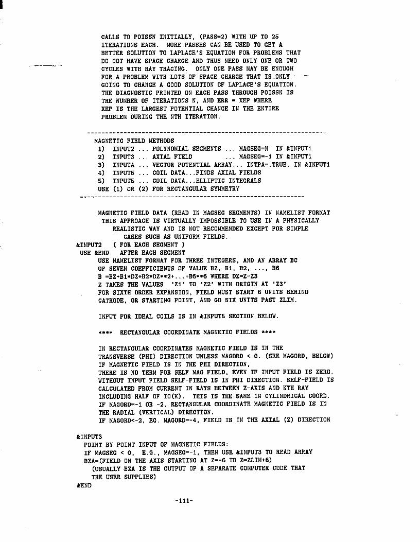
CALLS TO POISSN INITIALLY, (PASS=2) WITH UP TO 25 ITERATIONS EACH. MORE PASSES CAN BE USED TO GET A BETTER SOLUTION TO LAPLACE'S EQUATION FOR PROBLEMS THAT DO NOT HAVE SPACE CHARGE AND THUS NEED ONLY ONE OR TWO CYCLES WITH RAY TRACING. ONLY ONE PASS MAY BE ENOUGH FOR A PROBLEM WITH LOTS OF SPACE CHARGE THAT ISONLY - - GOING TO CHANGE A GOOD SOLUTION OF LAPLACE'S EQUATION. THE DIAGNOSTIC PRINTED ON EACH PASS THROUGH POISSN IS THE NUMBER OF ITERATIONS N, AND ERR = XEP WHERE XEP IS THE LARGEST POTENTIAL CHANGE IN THE ENTIRE PROBLEM DURING THE NTH ITERATION.

__________-_________---------------------------------------------- MAGNETIC FIELD METHODS

I) INPUT2 . . . POLYNOMIAL SEGMENTS . . . MAGSEG=N IN &INPUT1 2) INPUT3 . . . AXIAL FIELD . . . MAGSEG=-I IN &INPUT1 3) INPUTA . . . VECTOR POTENTIAL ARRAY... INTPA=.TRUE. IN &INPUT1 4) INPUT5 . . . COIL DATA...FINDS AXIAL FIELDS 5) INPUT5 . . . COIL DATA...ELLIPTIC INTEGRALS USE (I) OR (2) FOR RECTANGULAR SYMMETRY

____------_______-_--~~~~~~~~~~~---------~~~~~~~~~~~~---------

MAGNETIC FIELD DATA (READ IN MAGSEG SEGMENTS) IN NAMELIST FORMAT THIS APPROACH IS VIRTUALLY IMPOSSIBLE TO USE IN A PHYSICALLY

REALISTIC WAY AND IS NOT RECOMMENDED EXCEPT FOR SIMPLE CASES SUCH AS UNIFORM FIELDS.

&INPUT2 ( FOR EACH SEGMENT ) USE &END AFTER EACH SEGMENT

USE NAMELIST FORMAT FOR THREE INTEGERS, AND AN ARRAY BC OF SEVEN COEFFICIENTS OF VALUE BZ, Bl, B2, . . . . B6 B =BZ+Bl*DZ+B2*DZ**2+...+B6**6 WHERE DZ=Z-Z3 Z TAKES THE VALUES 'Zl' TO '22' WITH ORIGIN AT '23' FOR SIXTH ORDER EXPANSION, FIELD MUST START 6 UNITS BEHIND CATHODE, OR STARTING POINT, AND GO SIX UNITS PAST ZLIM.

INPUT FOR IDEAL COILS IS IN &INPUT5 SECTION BELOW.

**** RECTANGULAR COORDINATE MAGNETIC FIELDS ****

IN RECTANGULAR COORDINATES MAGNETIC FIELD IS IN THE TRANSVERSE (PHI) DIRECTION UNLESS MAGORD < 0. (SEE MAGORD, BELOW) IF MAGNETIC FIELD IS IN THE PHI DIRECTION, THERE IS NO TERM FOR SELF MAG FIELD, EVEN IF INPUT FIELD IS ZERO. WITHOUT INPUT FIELD SELF-FIELD IS IN PHI DIRECTION. SELF-FIELD IS CALCULATED FROM CURRENT IN RAYS BETWEEN Z-AXIS AND KTH RAY INCLUDING HALF OF IO(K). THIS IS THE SAME IN CYLINDRICAL COORD. IF MAGORD=-I OR -2, RECTANGULAR COORDINATE MAGNETIC FIELD IS IN THE RADIAL (VERTICAL) DIRECTION. IF MAGORDC-2, EG. MAGORD=-4, FIELD IS IN THE AXIAL (Z) DIRECTION

.-

&INPUT3 POINT BY POINT INPUT OF MAGNETIC FIELDS: IF MAGSEG < 0, E.G., MAGSEG=-1, THEN USE &INPUT3 TO READ ARRAY BZA=(FIELD ON THE AXIS STARTING AT Z=-6 TO Z=ZLIM+G)

(USUALLY BZA IS THE OUTPUT OF A SEPARATE COMPUTER CODE THAT THE USER SUPPLIES)

&END

-lll-

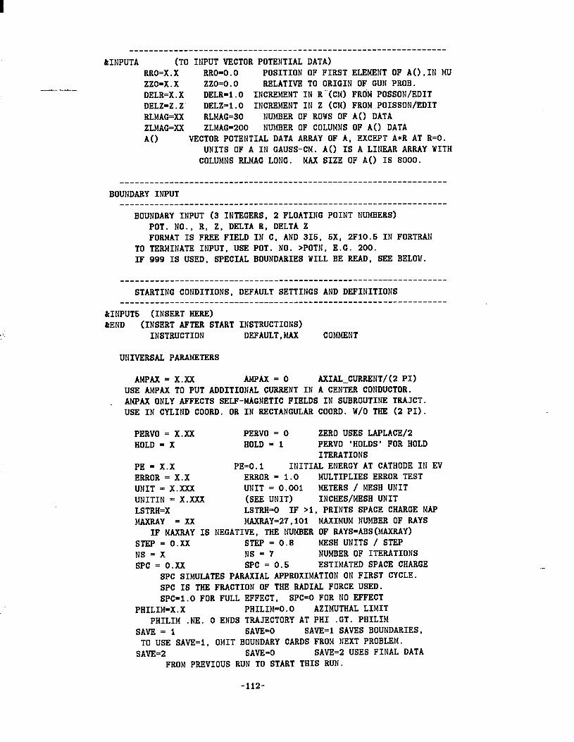
______________--____-------------------------------------------- &INPUTA (TO INPUT VECTOR POTENTIAL DATA)

RRO=X.X RRO=O.O POSITION OF FIRST ELEMENT OF A(),IN MU zzo=x . x zzo=o. 0 RELATIVE TO ORIGIN OF GUN PROB. DELR=X.X DELR=I.O INCREMENT IN R-(CM) FROM POSSON/EDIT DELZ=Z.Z DELZ-1.0 INCREMENT IN Z (CM) FROM.POISSUN/EDIT RLMAG=XX RLMAG=30 NUMBER OF ROWS OF A() DATA ZLMAG=XX ZLMAG=200 NUMBER OF COLUMNS OF A() DATA A0 VECTOR POTENTIAL DATA ARRAY OF A, EXCEPT A*R AT R=O.

UNITS OF A IN GAUSS-CM. A() IS A LINEAR ARRAY WITH COLUMNS RLMAG LONG. MAX SIZE OF A() IS 8000.

BOUNDARY INPUT ~~~~~~~----~~__--------~~~~~--------~~~~~-------~-~~~~~-~--------~

BOUNDARY INPUT (3 INTEGERS, 2 FLOATING POINT NUMBERS) POT. NO., R, Z, DELTA R, DELTA Z FORMAT IS FREE FIELD IN C, AND 315, 5X, 2F10.5 IN FORTRAN

TO TERMINATE INPUT, USE POT. NO. >POTN, E.G. 200. IF 999 IS USED, SPECIAL BOUNDARIES WILL BE READ, SEE BELOW.

--------~~__--------~~~~------~~~~~~~~~----~~~~~~~~~~~~~~~~ ------- STARTING CONDITIONS, DEFAULT SETTINGS AND DEFINITIONS

------~~~~~_-------~~~~~~~-------~-~~~~~~~~~--------~~~~~~~~~~~~~~ &INPUT5 (INSERT HERE) &END (INSERT AFTER START INSTRUCTIONS)

INSTRUCTION DRFAULT,MAX COMMENT

UNIVERSAL PARAMETERS

AMPAX = x.xX AMPAX=O AXIAL-CURRENT/(2 PI) USE AMPAX TO PUT ADDITIONAL CURRENT IN A CENTER CONDUCTOR. AMPAX ONLY AFFECTS SELF-MAGNETIC FIELDS IN SUBROUTINE TRAJCT. USE IN CYLIND COORD. OR IN RECTANGULAR COORD. W/O THE (2 PI).

PERVO = X.XX PERVO = 0 ZERO USES LAPLACE/% HOLD = X HOLD = I PERVO 'HOLDS' FOR HOLD

ITERATIONS PE = X.X PE=O.I INITIAL ENERGY AT CATHODE IN EV ERROR = X.X ERROR = 1.0 MULTIPLIES ERROR TEST UNIT = x.xXx UNIT = 0.001 METERS / MESH UNIT UNITIN = x.xXx (SEE UNIT) INCHES/MESH UNIT LSTRH=X LSTRH-0 IF >I, PRINTS SPACE CHARGE MAP MAXRAY =X.X MAXRAY=27,101 MAXIMUM NUMBER OF RAYS

IF MAXRAY IS NEGATIVE, THE NUMBER OF RAYS=ABS(MAXRAY) STEP = 0.xX STEP = 0.8 MESH UNITS / STEP NS = X NS = 7 NUMBER OF ITERATIONS SPC = o.XX SPC = 0.5 ESTIMATED SPACE CHARGE

SPC SIMULATES PARAXIAL APPROXIMATION ON FIRST CYCLE. SPC IS THE FRACTION OF THE RADIAL FORCE USED. SPC=I.O FOR FULL EFFECT, SPC=O FOR NO EFFECT

PHILIM=X.X PHILIM=O.O AZIMUTHAL LIMIT PHILIM .NE. 0 ENDS TRAJECTORY AT PHI .GT. PHILIM

SAVE = I SAVE-O SAVE-1 SAVES BOUNDARIES, TO USE SAVE=I, OMIT BOUNDARY CARDS FROM NEXT PROBLEM.

SAVE=2 SAVE-O SAVE=2 USES FINAL DATA FROM PREVIOUS RUN TO START THIS RUN.

-112-

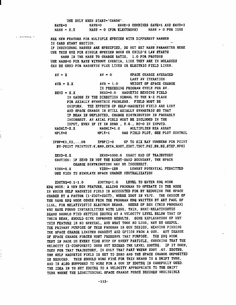
USE ONLY WHEN START='CARDS'. SAVE=3 SAVE=0 SAVE=3 COMBINES SAVE-I AND SAVE=2 MASS = x.x MASS = 0 (FOR ELECTRONS) MASS > 0 FOR IONS

SEE NEW FEATURE FOR MULTIPLE SPECIES WITH DIFFERENT MASSES IN CARD START SECTION. - . IF INDIVIDUAL MASSES ARE SPECIFIED, DO NOT SET MASS PARAMETER HERE USE THIS ONE FOR SINGLE SPECIES RUNS OR CHILD'S LAW STARTS

MASS IS THE MASS TO CHARGE RATIO, 1.0 FOR PROTONS USE MASS<0 FOR RAYS WITHOUT INERTIA, LIKE THEY ARE IN MOLASSES CAN BE USED FOR MAGNETIC FLUX LINES OR ELECTRIC FIELD LINES.

AV = X AV = 0 SPACE CHARGE AVERAGED LAST AV ITERATION

AVR = X.X AVR = 1.0 WEIGHT OF SPACE CHARGE IN PRECEDING PROGRAM CYCLE FOR AV.

BEND = X.X BEND-O.0 MAGNETIC BENDING FIELD IN GAUSS IN THE DIRECTION NORMAL TO THE R-Z PLANE FOR AXIALLY SYMMETRIC PROBLEMS. FIELD MUST BE UNIFORM. THE EFFECTS OF SELF-MAGNETIC FIELD ARE LOST AND SPACE CHARGE IS STILL AXIALLY SYMMETRIC SO THAT IF BEAM IS DEFLECTED, CHARGE DISTRIBUTION IS PROBABLY INCORRECT. AN AXIAL FIELD MUST BE INCLUDED IN THE INPUT, EVEN IF IT IS ZERO , E.G., BC=O IN INPUTP.

MAGMLT=X.X MAGMLT=I.O MULTIPLIES BZA ARRAY MPLT=X MPLT-I MAC FIELD PLOT, SEE PLOT CONTROL

IPBP=KI,KZ,...KG IPBP()=O up TO SIX RAY NUMBERS FOR POINT BY-POINT PRINTOUT:K,RHO,ZETA,RDOT,ZDOT,TDOT,PHI,BR,BZ,STEP,BPHI

ZEND=X.X ZEND-1000.0 EXACT END OF TRAJECTORY CAUTION: IF ZEND IS NOT THE RIGHT-HAND BOUNDARY, THE SPACE

CHARGE DISTRIBUTION MAY BE INCORRECT. VION=X.X VION=-IE8 LOWEST POTENTIAL PERMITTED USE VION TO SIMULATE SPACE CHARGE NEUTRALIZATION

ZDOTEQ=O.I-1.0 ZDOTEQ-1.0 LEVEL TO ENTER EBQ MODE EBQ MODE: A NEW EGN FEATURE, ALLOWS PROGRAM TO OPERATE IN THE MODE IN WHICH SELF MAGNETIC FIELD IS ACCOUNTED FOR BY REDUCING THE SPACE CHARGE BY A FACTOR (I-ZDOT*ZDOT), WHERE ZDOT IS VZ/C. THE CHOICE OF THE NAME EBQ MODE COMES FROM THE PROGRAM EBQ WRITTEN BY ART PAUL OF LLNL, FOR RELATIVISTIC ELECTRON BEAMS. usERs OF EGN (THIS PROGRAM) WHO HAVE FOUND INSTABILITIES WITH LONG, THIN, SEMI-RELATIVISTIC BEAMS SHOULD FIND SETTING ZDOTEQ AT A VELOCITY LEVEL BELOW THAT OF THEIR BEAM, SHOULD GIVE IMPROVED RESULTS. SOME EXPLANATION OF WHY THIS FEATURE IS SO SPECIAL, AND WHAT TOOK SO LONG, MAY BE USEFUL. THE PRIMARY PURPOSE OF THIS PROGRAM IS GUN DESIGN, MEANING FINDING THE SPACE CHARGE LIMITED CURRENT AND OPTICS FROM A GUN. ANY CHANGE OF SPACE CHARGE FORCES MUST PRESERVE THAT PURPOSE. THE EBQ MODE TEST IS MADE ON EVERY TIME STEP OF EVERY PARTICLE, CHECKING THAT THE VELOCITY (Z-COMPONENT) DOES NOT EXCEED THE LEVEL ZDOTEQ. IF IT DOES, THEN FOR THAT TRAJECTORY, IN ONLY THAT PART WHERE ZDOT .GT. ZDOTEQ, THE SELF MAGNETIC FIELD IS SET TO ZERO AND THE SPACE CHARGE DEPOSITED IS REDUCED. THIS SHOULD WORK FINE FOR THIN BEAMS IN A DRIFT TUBE, AND IS ALSO SUPPOSED TO WORK FOR A GUN IF ZDOTEQ IS CAREFULLY USED. THE IDEA IS To SET ZDOTEQ TO A VELOCITY APPROPRIATE TO THE DRIFT TUBE WHERE THF, LONGITUDINAL SPACE CHARGE FORCE BECOMES NEGLIGIBLE

-113-

AND THE TRANSVERSE FOCUSING BECOMES A BALANCE OF FORCES BETWEEN SELF-MAGNETIC FIELDS AND SPACE CHARGE. USERS SHOULD CONSIDER THIS FEATURE AS A KNOB TO EXPERIMENT WITH.

____________________---------------------------------------------- INPUT FOR EQUIPOTENTIAL PLOTS - ____________________----------------------------------------------

EQUIPR = X.X EQUIPR = 0.0 R-INTERSECTION FOR EQUIPOTENTIAL LINES

LM = XXX LM = 300 LENGTH OF EQUIPOTENTIALS EQLN = 0 TO 20 EQLN = I NO. OF CORRECTIONS EQST = X EQST = 2 STEPS PER MESH UNIT

Izl=x,Iz2=x,Izs=x 1z1=0,1z2=-I EXTRA EQUIPOTENTIALS AT IZS=IO THE INDICATED VALUES OF Z.

EQUIPOTENTIAL LINES ARE DRAWN AT 5, 15, 25.......85, 95 PERCENT OF DIFFERENCE BETWEEN POT(2) AND POT(I). ALSO LINES ARE AT 20, 40, 60, 80 AND 100 PERCENT OF DIFFERENCE BETWEEN POT(3) AND POT(l).

____________________---------------------------------------------- PLOTTING CONTROLS ____________________----------------------------------------------

SCALE = 'YES' SCALE - ' ' 'YES'- DIFFERENT X,Y SCALE sx = xx SX = 8 HORIZONTAL PLOT WIDTH (INCHES) SY = xx SY = 9 VERTICAL PLOT HEIGHT (INCHES) IPHI =X.X IPHI = 0 DESIGNATES A SINGLE

TRAJECTORY FOR A PHI VS Z PLOT

MPLT=X MPLT=I IF =I, PLOT AXIAL FIELD, AT R=O 11 =O, SUPPRESS MAG FIELD PLOT 11 '2, PLOT BZ AT R = RMAG II =3, PLOT BR AT R = RMAG

DATA FOR POST PROCESSORS IS SAVED IN A BINARY FILE. SPECIFY IZSAVI, IZSAVP AND IZSAVS FOR A LOOP FROM Z=IZSAVI TO Z=IZSAV2 IN STEPS OF IZSAVS. AT THE NEXT INTEGRAL STEP AFTER ZETA=Z, THE DATA SAVED INCLUDES Z, K(ray number), IO(current), RHO, ZETA, RDOT, ZDOT. TDOT, BR, BZ and BPHI.

POST PROCESSORS CAN BE CUSTOMIZED TO PARTICULAR APPLICATIONS. EXAMPLES ARE: READ AND PRINT DATA SORTED BY Z, CALCULATE WAISTS AND EMITTANCES, DO SPECIAL CALCULATIONS FOR GYROTRONS.

------_-----_----__---~~----~~----- ------_-----_------_-----~----- MAGNETIC FIELDS; METHOD ONE; READ IN AXIAL FIELD IN SECTION 3(ABOVE) _--_________-_____-_------------ ------__---___---__----~~---~~~~--

RMAG = x.x RMAG = RLIM/P OFF-AXIS MAGNETIC FIELD (RMAG ONLY AFFECTS THE LISTING) AT R=RMAG

MAGORD = 2,4 MAGORD = 6 HIGHEST ORDER FIELD TERM IF MAGORD=-I OR -2 FOR RECTANGULAR COORDINATES, BZA IS IN THE

R-DIRECTION AND THE OFF-AXIS EXPANSION IS A FUNCTION OF R. IF MAGORDC-2 FOR RECTANGULAR COORDINATES, BZA IS IN THE

Z-DIRECTION AND THE EXPANSION IS ALSO A FUNCTION OF R. EXPANSIONS IN RECTANGULAR COORDINATES ARE TO SECOND ORDER ONLY.

NMAG = X NMAG = 0,101 NO. OF FIELD COILS FOR METHOD TWO __________--__--------- __--_--- _---_-- _---_--- _--__--_----v--e----

-114-

METHOD TWO; READ IN POSITION AND STRENGTH OF NMAG IDEAL COILS. IF NELL=O, PROGRAM CALCULATES BZA ARRAY AND PROCEEDS AS IN METHOD ONE IF NELL=l, THIS METHOD CALCULATES FIELDS USING THE COMPLETE ELLIPTIC INTEGRAL FUNCTIONS. FIELDS ARE THEN VALID IN ALL SPACE.

**** THIS VERSION INCLUDES SERIES EXPANSIONS FOR THE INTEGRALS *** IF MANY COILS ARE USED, THE ELLIPTIC INTEGRALS WILL.SLOW EXECUTION

IF COIL INPUTS ARE USED FOR MAGNETIC FIELDS. THE PROGRAM WILL LIST THE OFF-AXIS FIELDS BY BOTH OFF-AXIS EXPANSIONS AND BY USING ELLIPTIC INTEGRALS, AT R=RMAG, EVEN IF NELL=O. THIS PROVIDES AN INTERESTING CHECK ON THE VALIDITY OF THE OFF-AXIS EXPANSIONS IN THE USER'S SPECIAL SITUATION.

NELL=1 NELL=O, =I FOR ELLIPTIC INTEGRALS CR(I) = X.X CR(I) = RLIM RADIUS OF COIL (MESH UNIT) CZ(1) = x.x czw = 0.0 AXIAL POSITION OF COIL CM(I) = X.X CM(I) = 0.0 CURRENT IN AMPERE-TURNS

THE NELL=0 CASE CAN BE USED FOR STRAIGHT WIRES IN RECT. COORDINATES. ------------------------------------------------------------------

START GENERAL ----------~~~~~~~------------~~~~~~~~~~----------~-~-----~--~~--~~

START = 'GENERAL' START = 'GENERAL' GENERAL CATHODE RC = X.XX RC = 0.0 LOWER END OF STARTING SURFACE zc = x.xX zc = 2+CATHODEZ CATHODEZ IS Z VALUE OF

BOUNDARY FROM FIRST DATA CARD. CL = x.xX CL = RLIM MAXIMUM LENGTH OF STARTING

SURFACE DENS = xX.x DENS = 100.0 MAXIMUM EMISSION (A/CM**2) BETA2 = 1.0 BETA2= 0.0 IF > 0.0 USES LANGMUIR-

BLODGETT FORMALISM RAD = X.X --- USE RAD FOR WIRE RADIUS IN

RECTANGULAR COORDINATES, BETA2 > 0.0

SURFAC = X SURFAC -1 STARTING SURFACE ITERATION _____-------~-~~~~~~~------~~~~~~~~~~~~~~ USE POT(5) FOR NON-EMITTING SURFACE, E.G. HOLLOW CATHODE OR SHADOW GRID. DO NOT USE POT(3) OR POT(5) FOR FOCUS ELECTRODE . . . USE POT(4) TO STOP ELECTRONS ON IMPACT.

________________-___---------------------------------------------- START GENCARD ___________-------_-------~-~~~~~~~~ __________----------~~~~~~~~~~

START = 'GENCARD' START = 'GENERAL' GENERAL WITH CARD START

HAVE up TO MAXRAY CARDS WHICH SPECIFY: I) RAY NO. 2) MASS, 0.0 FOR ELECTRONS 3) INITIAL RADIUS R 4) INITIAL AXIAL VALUE Z 5) DISTANCE FROM CATHODE DX (CATHODE MUST BE POT(~)). 6) EFFECTIVE SPACING BETWEEN RAYS DR. 7) PARAMETER WHICH MODIFIES CHILD LANGMUIR EQUATION, ALPH2.

NORMAL DX IS 1.0 TO 2.0 MESH UNITS. NORMAL DR IS 1.0 BUT MAY BE VARIED ALONG THE SURFACE. NORMAL ALPHZ IS 1.0 FOR A PLAIN DIODE.

FOR CYLINDRICAL COORDINATES: ALPHZ=(ALPHA*(RADIUS OF CURVATURE)/(STARTING STEP))**2

-115-

FOR RECTANGULAR COORDINATES: ALPH2=(BETA**2)*(RADIUS OF CURVATURE)/(STARTING STEP) WHERE ALPHA AND BETA ARE AS DEFINED IN THE LITERATURE,E.G., SPANGENBERG FOR BETA AND BREWER IN SEPTIER, VOL II, FOR ALPHA FORMAT IS FREE FIELD; RAY NO.,MASS,R,Z,DX,DR,ALPH2

____-------~-~~~~------------~~~~~-~-------~~~~~~~~~~~~~~~~~~~~~~~ START SPHERE _ - . . _______________--_______________________--------------------------

START = 'SPHERE' START = *GENERAL' SPHERICAL CATHODE RAD = x.xX RAD = 2*ZLIM SPHERICAL RADIUS RMAX = X.XX RMAX = RLIM CATHODE RADIUS ORAD = X.xX ORAD = CATHODEZ CENTER OF CATHODE ST = X.XX ST = 2.0 STARTING STEP

--------------------------------~~~~~~~~- 'SPHERE' ALSO WORKS FOR CYLINDRICAL CATHODE IN RECTANGULAR COORDINATES ______---------~~___------------~~~~~~----------~~~~~~~~~~~~~~~~~~ START CARDS ______________---___----------------------------------------------

START = 'CARDS' START = 'GENERAL' CARD STARTING zo = x.xX zo = 0.0 OLD ORIGIN IN NEW FRAME SKAL = x.xX SKAL = 1.0 OLD MESH/NEW MESH

HAVE UP TO MAXRAY DATA CARDS (I INTEGER, 8 FLOATING POINT) RAY, MASS, R, Z. ENERGY(EV), ANGLE(RADIANS), CURRENT(MICROAMPERES IN ONE RADIAN SEGMENT), TRANSVERSE ANGLE. TRANSVERSE POSITION(PH1) FREE FIELD FORMAT IN C REQUIRES NINE (9) ENTRIES PER TRAJECTORY.

STOP READING WITH RAY NO. GREATER THAN MAXRAY. INITIAL TRANSVERSE VELOCITY HAS THE SIGN OF THE TRANSVERSE ANGLE

** NEW EGN FEATURE; MASS MUST BE SPECIFIED FOR EACH RAY. ** PUT MASS ON CARD START DATA AFTER RAY NUMBER. ** NOTE THAT ELECTRONS HAVE MASS CODE NUMBER = 0. PROTONS MASS=I. ** USE NEGATIVE CURRENTS FOR POSITIVE IONS. *' MASS=l.5 WOULD BE LIKE DOUBLY CHARGED TRITIUM.

IF CURRENT IS NEGATIVE, POSITIVE CHARGE IS ACCELERATED. THIS CAN BE USED TO TRACK IONS IN THE FIELDS FROM AN ELECTRON BEAM PROBLEM (USE SAVE=I) OR SECONDARY ELECTRONS FROM AN ION BEAM PROBLEM.

IF RECTANGULAR COORDINATES: I) PHI IS TRANSVERSE POSITION IN MESH UNITS. 2) CURRENT IS MICROAMPERES IN ONE MESH UNIT DEEP SEGMENT.

CARDS SHOULD BE SORTED ACCORDING TO INITIAL VALUE OF RHO. USE IRAT=I TO DEFEAT THE BUILT IN SORT ROUTINE WHICH SEQUENCES RAYS

****SPECIAL TESTS IN RATNST; CROSSING OR 3-D SPACE CHARGE** IRAT=l IRAT=O 3-D SPACE CHARGE IRAT= IRAT-O CROSSING DETECTION

USE OF NEGATIVE RAY NUMBERS: A) IF IRAT=I (3-D SPACE CHARGE)

I) MAKE RAY NUMBERS NEGATIVE FOR BEAM EDGE CARDS. USE BEAM EDGE CARDS (IO-O) TO SIMULATE SPACE CHARGE SPREADING OF A CYLINDRICAL BEAM OF CURRENT I AND RADIUS R IN RECT. COORD.

PAIRS OF BEAM EDGE CARDS PRECEDE SETS OF RAY CARDS DEFINING PART OF BEAM IN WHICH 3-D SPACE CHARGE SPREAD IS TO BE SIMULATED SEVERAL PARTS, DIFFERENTIATED BY SELECTED ATTRIBUTES; EG., ENERGY, ALPHA OR RADIUS, CAN BE USED SIMULTANEOUSLY WITH ANY NUMBER OF RAYS IN EACH PART. END OF PART IS DEFINED BY NEXT RAY WITH NEGATIVE RAY NUMBER, WHICH BEGINS THE NEXT PART.

-116-

2) TO SIMULATE CYLINDRICAL BEAM SPACE CHARGE IN RECTANGULAR COORDINATES MAKE CURRENT PER MESH UNIT, I' = I/(PI*R) INSTEAD OF I' = 2*I/(PI*R) WHICH WOULD HAVE THE SAME CURRENT DENSITY. IN OTHER WORDS, MAKE I'(K) = I(K) / (2*R(K)) INSTEAD OF I(K)/ R(K). NOTE THAT THIS REQUIRES TWICE AS MANY RAYS AS FOR CYLINDRICAL BEAM WITH SYMMETRY. BEAM EDGE CARDS (RAY NO. < 0) ALSO APPLY TO OFF-AXIS PENCIL IN CYLINDRICAL COORDINATES.-

B) IF IRAT= (R-Z AND PHI CROSSOVERS) I) R-Z: MAKE RAY NUMBERS NEGATIVE FOR SEQUENTIAL RAYS FOR

WHICH FINAL CROSSOVER SHOULD BE DETECTED. CROSSINGS WILL BE LISTED AND PLOTTED. NEGATIVE RAY NUMBERS SHOULD BE IN PAIRS. TO FIND CROSSOVERS WITH Z AXIS, RUN A RAY WITH R=O,ALPHA=O PRECEDING THE RAY TO TEST AXIS CROSSING.

2) PHI: LEAVE RAY NUMBERS POSITIVE FOR TRANSVERSE RAYS TO DETECT LAST CROSSING OF PHI=PI*INTEGER.

IF SAVE=2, RUN STARTS WITH FINAL RAY DATA FROM PREVIOUS RUN. DO NOT PUT SAVE=2 ON THE FIRST RUN OF A SET.

--------------~~~~~~~~~~~~~~~~~~~--------~~~~~~~~~~~~~~~~~~~~~~~~~ THERMAL EFFECTS ------------------------------------------------------------------

SUBROUTINE THERM IS CALLED IF THE PARAMETER TC>O. TC=XXXX . X TC=O KELVIN TEMP. OF CATHODE THREE MODELS ARE INCLUDED IN THIS VERSION KRAY=2 KRAY=I TWO RAY SPLIT, RANDOMIZED KRAY=3 KRAY=l THREE RAY SPLIT KRAY=S KRAY=l FIVE RAY SPLIT

TWO RAY SPLIT DIVIDES CURRENTS EQUALLY INTO 2 RAYS WITH EQUAL ANGULAR DEVIATIONS FROM THE INITIAL DIRECTION. THE AMOUNT OF THE DEVIATION FOLLOWS A RANDOMIZED DISTRIBUTION BASED ON A ONE- DIMENSIONAL RMS DISTRIBUTION.

THREE RAY SPLIT PUTS CURRENTS IN 1-2-I RATIO WITH 2 PARTS IN UNDEFLECTED RAY AND I PART EACH IN RAYS WITH V(PERP)=SQRT(PKT/M) IN R-Z PLANE, UP AND DOWN RELATIVE TO UNDEFLECTED RAY.

FIVE RAY SPLIT PUTS CURRENTS IN 1-5-8-5-1 RATIO WITH V(PERP)=2*SQRT(2KT/M) FOR 1 PART RAYS AND V(PERP)=l*SQRT(2KT/M) FOR 5 PART RAYS. NO DEVIATION FOR CENTER 8-PART RAY.

THERM CAN BE CALLED FOR START='SPHERE', 'GENERAL', 'CARDS', OR 'GENCARD'. IT CANNOT BE USED FOR START='CARDS' WITH SAVE=2.

START LAPLACE

START = 'LAPLACE' START = 'GENERAL' NO RAY TRACING NS = X NS = 7 NUMBER OF LAPLACE CYCLES LAPRH=I LAPRH=O USE LAPRH=I TO START READING

DATA CARDS WITH (R,Z, SPACE CHARGE) FOR NON-ZERO POINTS. FREE FIELD FORMAT. END CARD INPUT WITH ANY SINGLE NUMBER.

FOR A BEAM GOING NORMAL TO THE R-Z PLANE, SPACE CHARGE IS RO(R,Z)=-120*PI*I/AREA(MU**2)*BETA....IN RECTANGULAR COORD.

WHERE AREA(SQ. MESH UNITS) FOR A UNIFORM BEAM OF CURRENT I(A). *****LAPRH IS A NEW INPUT FEATURE*****

PRINTED OUTPUT INCLUDES A TABLE OF SURFACE CHARGE FOR EACH SURFACE # (POT #). TO FIND CAPACITANCE, DIVIDE BY VOLTAGE.

-117-

________________----------------------------------------- --------

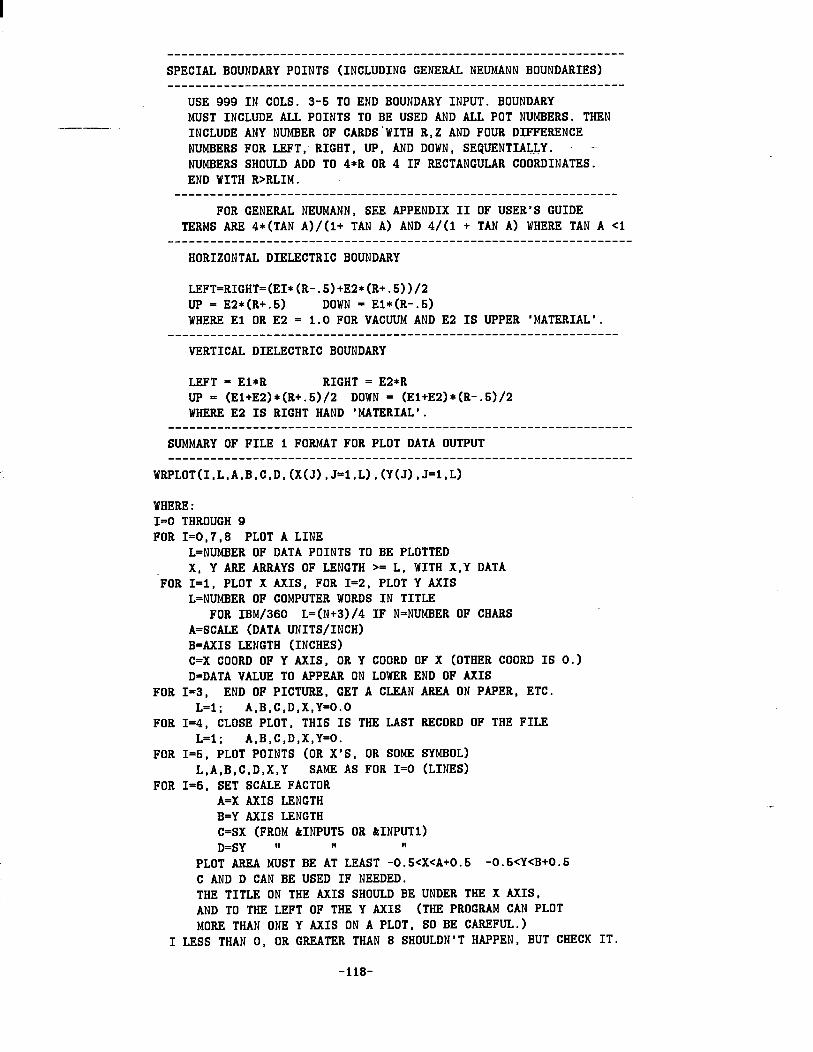
SPECIAL BOUNDARY POINTS (INCLUDING GENERAL NEUMANN BOUNDARIES) ---------~~~~~~~-------------~-~~~~~~------------------~~~~~~-~~~

USE 999 IN COLS. 3-5 TO END BOUNDARY INPUT. BOUNDARY MUST INCLUDE ALL POINTS TO BE USED AND ALL POT NUMBERS. THEN INCLUDE ANY NUMBER OF CARDS'WITH R,Z AND FOUR DIFFERENCE NUMBERS FOR LEFT, RIGHT, up, AND DOWN, SEQUENTIALLY. - - NUMBERS SHOULD ADD TO 4*R OR 4 IF RECTANGULAR COORDINATES. END WITH R>RLIM.

________________----------------------------------------- ------ FOR GENERAL NEUMANN, SEE APPENDIX II OF USER'S GUIDE

TERMS ARE 4*(TAN A)/(l+ TAN A) AND 4/(1 + TAN A) WHERE TAN A <l ------------~-~~~___~------------~~~~~~~~~~~~~~--~----------------

HORIZONTAL DIELECTRIC BOUNDARY

LEFT=RIGHT=(EI*(R-.5)+E2*(R+.5))/2 UP = E2*(R+.5) DOWN = El*(R-.5) WHERE El OR E2 = 1.0 FOR VACUUM AND E2 IS UPPER 'MATERIAL'.

__---------_______---~~~~~~~~~~~~~~~-------~~~~~~~~~~~~~~~~-~--- VERTICAL DIELECTRIC BOUNDARY

LEFT = EI*R RIGHT = E2*R UP= (El+E2)*(R+.5)/2 DOWN = (El+E2)*(R-.5)/2 WHERE E2 IS RIGHT HAND 'MATERIAL'.

---------~~~~~~~~~~~~~~~~~~~~~~~~-~~~~~~~~~~~~~~~~~~~~~~~~~~~~~~~~ SUMMARY OF FILE I FORMAT FOR PLOT DATA OUTPUT ________________--------------------------------------------------

WRPLOT(I,L,A,B,C,D,(X(J),J=I,L),(Y(J),J=l,L)

WHERE: I=0 THROUGH 9 FOR 1=0,7,8 PLOT A LINE

L=NUMBER OF DATA POINTS TO BE PLOTTED X. Y ARE ARRAYS OF LENGTH >= L, WITH X,Y DATA

-FOR I=l, PLOT X AXIS, FOR 1=2, PLOT Y AXIS L-NUMBER OF COMPUTER WORDS IN TITLE

FOR IBM/360 L=(N+3)/4 IF N-NUMBER OF CHARS A=scALE (DATA UNITS/INCH) B-AXIS LENGTH (INCHES) c=x cooRD OF Y AXIS, OR Y COORD OF x (OTHER COORD IS 0.) D-DATA VALUE TO APPEAR ON LOWER END OF AXIS

FOR 133, END OF PICTURE, GET A CLEAN AREA ON PAPER, ETC. L=l; A,B,C,D,X,Y=O.O

FOR 1=4, CLOSE PLOT, THIS IS THE LAST RECORD OF THE FILE L=l; A,B,C,D,X,Y=O.

FOR 1=5, PLOT POINTS (OR X'S, OR SOME SYMBOL) L,A,B,C,D,X,Y SAME AS FOR I=O (LINES)

FOR I-6, SET SCALE FACTOR A=X AXIS LENGTH B-Y AXIS LENGTH c=sx (FROM &INPUTS OR ~INPUT~) D=SY w w ,,

PLOT AREA MUST BE AT LEAST -0.5<X<A+0.5 -O.S<Y<B+O.S C AND D CAN BE USED IF NEEDED. THE TITLE ON THE AXIS SHOULD BE UNDER THE X AXIS, AND TO THE LEFT OF THE Y AXIS (THE PROGRAM CAN PLOT MORE THAN ONE Y AXIS ON A PLOT, SO BE CAREFUL.)

I LESS THAN 0, OR GREATER THAN 8 SHOULDN'T HAPPEN, BUT CHECK IT.

-118-

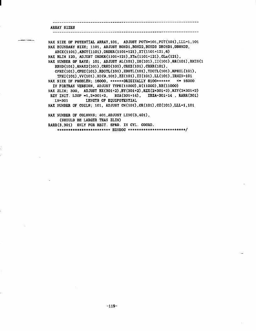
MAX SIZE OF POTENTIAL ARRAY.101, ADJUST POTN=IOI,POT(IOI),LLL=l,lOl MAX BOUNDARY SIZE; 1101, ADJUST BONDI,BONDZ,BOND3 DBoNRl,DBOND%,

~cx(llOl),~CY(llOl),ORDER(llOl+l2l),XT(llOl+l2l,6) MAX RLIM 120, ADJUST 0RDER(1101+121),XTn(1101+121),CLn(121), MAX NUMBER OF RAYS; 101, ADJUST AL(lOl),IO(lOl),II(lOl),RR(lOl),RMIN(I

~ND(lOl),RMAX2(lOl),CRHO(lOl),CRHZ(lOl),CRHR(lOl), CPHZ(lOl),CPHI(lOl),RDOTL(lOl),ZDOTL(lOl),TDOTL(lOl),~HIL(lOl),

TPHI(lOl>,W(lOl),XO(9,lOl),ZZ(lOl),II(lOl),LL(lOl),IRMIN=lOl MAX SIZE OF PROBLEM; 16000, ******ORIGINALLY 8100****** <= 16000

IN FORTRAN VERSION, ADJUST TYPE(llOOO),U(llOOO),RH(llOOO) MAX ZLIM; 300, ADJUST BX(301+2),BY(301+2),RZX(2*301+2),RZY(2*301+2)

RZY INIT. LOOP =1,2*301+2, BZA(301+14), IBZA=301+14 , RARR(301) LM-301 LENGTH OF EQUIPOTENTIAL

MAX NUMBER OF COILS; 101, ADJUST CM(lOl),CR(lOl),CZ(lOl),LLL=l,lOl

MAX NUMBER OF COLUMNS; 401,ADJUST LINC(3,401), (SHOULD BE LARGER THAN ZLIM)

RARR(3,301) ONLY FOR RECT. SPRD. IN CYL. COORD. ************************ EGNDOC **************************/

-119-

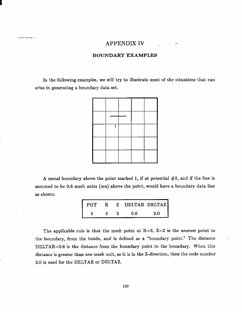
APPENDIX IV ._ -

BOUNDARY EXAMPLES

arise in generating a boundary data set.

In the following examples, we will try to illustrate most of the situations that can

A metal boundary above the point marked 1, if at potential #3, and if the line is

assumed to be 0.6 mesh units (mu) above the point, would have a boundary data line

as shown:

The applicable rule is that the mesh point at R=3, Z=2 is the nearest point to

the boundary, from the inside, and is defined as a “boundary point.” The distance

DELTAR=0.6 is the distance from the boundary point to the boundary. When this

distance is greater than one mesh unit, as it is in the Z-direction, then the code number

2.0 is used for the DELTAR or DELTAZ.

-

120

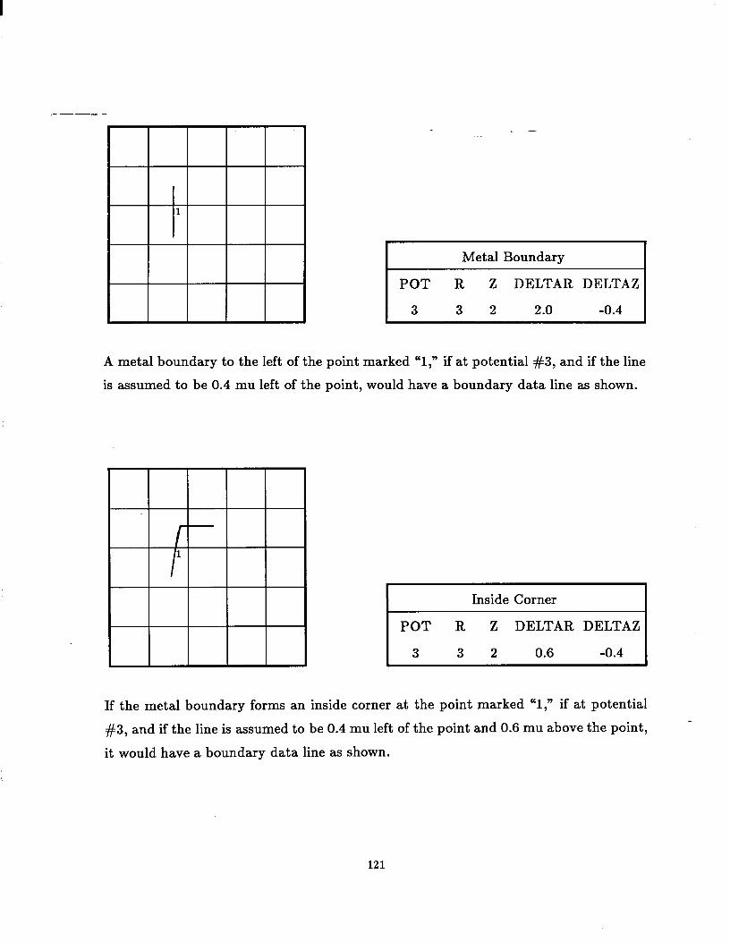
Metal Boundary

POT R Z DELTAR DELTAZ

3 3 2 2.0 -0.4

A metal boundary to the left of the point marked “1, n if at potential #3, and if the line

is assumed to be 0.4 mu left of the point, would have a boundary data line as shown.

I Inside Corner I

POT R Z DELTAR DELTAZ

3 3 2 0.6 -0.4

If the metal boundary forms an inside corner at the point marked “1,” if at potential

#3, and if the line is assumed to be 0.4 mu left of the point and 0.6 mu above the point,

it would have a boundary data line as shown.

--

121

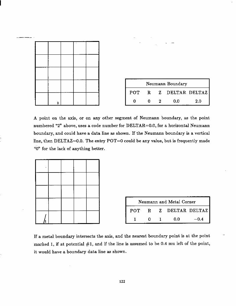
A point on the axis, or on any other segment of Neumann boundary, as the point

numbered “2” above, uses a code number for DELTAR=O.O, for a horizontal Neumann

boundary, and could have a data line as shown. If the Neumann boundary is a vertical

line, then DELTAZ=O.O. The entry POT=0 could be any value, but is frequently made

“0” for the lack of anything better.

If a metal boundary intersects the axis, and the nearest boundary point is at the point

marked 1, if at potential #l, and if the line is assumed to be 0.4 mu left of the point,

it would have a boundary data line as shown.

122

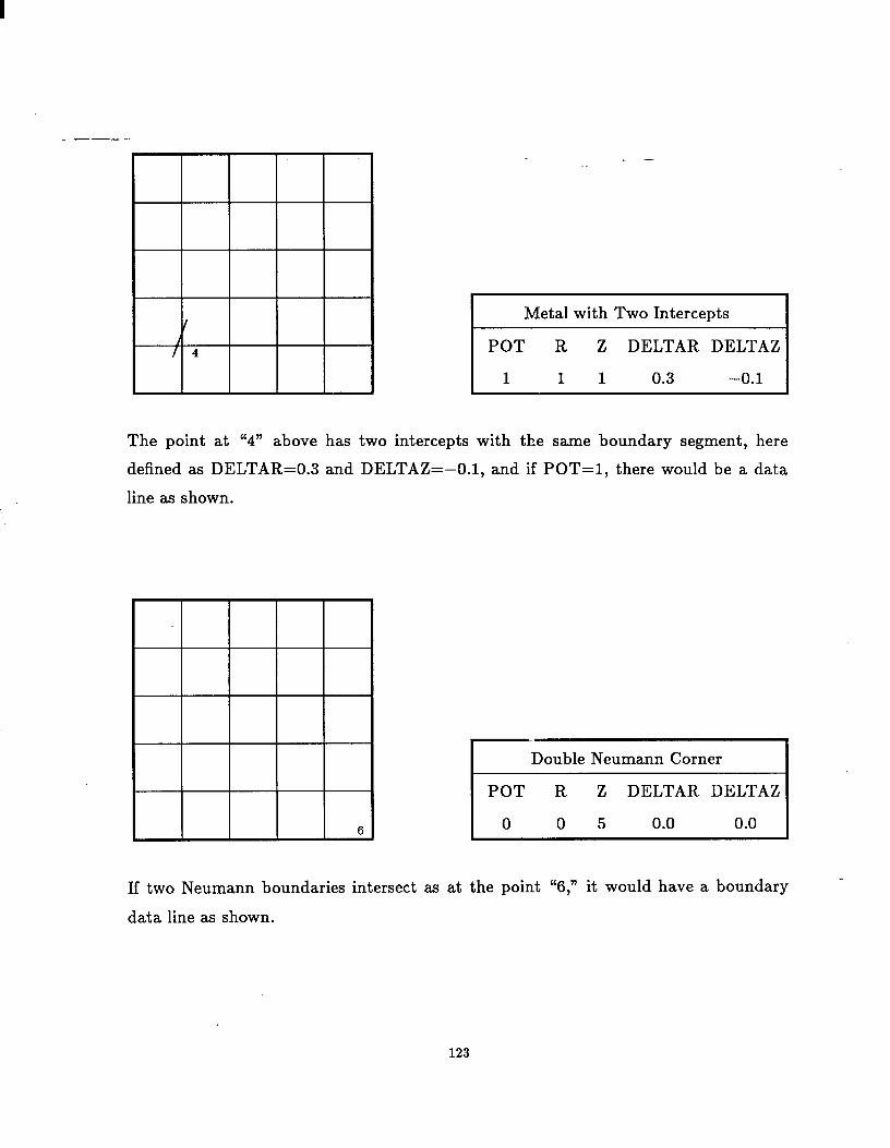
Metal with Two Intercepts

POT R Z DELTAR DELTAZ

1 1 1 0.3 -0.1

The point at “4” above has two intercepts with the same boundary segment, here

defined as DELTAR=0.3 and DELTAZ=-0.1, and if POT=l, there would be a data

line as shown.

Double Neumann Corner

POT R Z DELTAR DELTAZ

0 0 5 0.0 0.0

If two Neumann boundaries intersect as at the point “6,” it would have a boundary

data line as shown.

.-

123

0 1

2

Outside Corner

POT R Z DELTAR DELTAZ

2 3 3 -0.4 2.0

2 2 2 2.0 0.3

The outside corner in the figure above requires the two boundary points at “1” and “2”

to be defined. The point marked “0” is not a boundary point...the boundary does not

intercept the mesh within one mesh unit of the point marked “0.” If the sharp corner

is potential #2, the boundary data for the points at “1" and “2” are respectively as

shown.

I Thin Foil or Ideal Grid I

I POT R Z DELTAR DELTAZ

3 3 2 2.0 0.4

3 2 2 2.0 0.4

3 2 3 2.0 -0.6

3 3 3 2.0 -0.6

A thin sheet, or ideal grid, at potential #3, must be defined on both sides as shown.

124

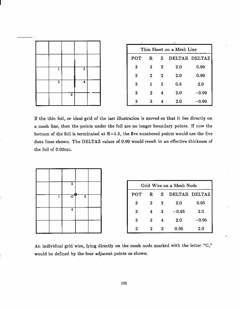
I Thin Sheet on a Mesh Line

POT R Z DELTAR DELTAZ

3 3 2 2.0 0.99

3 2 2 2.0 0.99

3 13 0.5 2.0

3 2 4 2.0 -0.99

3 3 4 2.0 -0.99

If the thin foil, or ideal grid of the last illustration is moved so that it lies directly on

a mesh line, then the points under the foil are no longer boundary points. If now the

bottom of the foil is terminated at R=1.5, the five numbered points would use the five

data lines shown. The DELTAZ values of 0.99 would result in an effective thickness of

the foil of 0.02mu.

Grid Wire on a Mesh Node

POT R Z DELTAR DELTAZ

3 3 2 2.0 0.95

3 4 3 -0.95 2.0

3 3 4 2.0 -0.95

3 2 3 0.95 2.0

- /

An individual grid wire, lying directly on the mesh node marked with the letter “G,”

would be defined by the four adjacent points as shown.

125

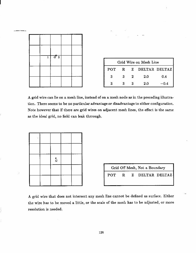
A grid wire that does not intersect any mesh line cannot be defined as surface. Either

the wire has to be moved a little, or the scale of the mesh has to be adjusted, or more

resolution is needed.

Grid Wire on Mesh Line

POT R Z DELTAR DELTAZ

3 3 2 2.0 0.4

3 3 3 2.0 -0.4

A grid wire can lie on a mesh line, instead of on a mesh node as in the preceding illustra-

tion. There seems to be no particular advantage or disadvantage to either configuration.

Note however that if there are grid wires on adjacent mesh lines, the effect is the same

as the ideal grid, no field can leak thrrough.

Grid Off Mesh, Not a Boundary

POT R Z DELTAR DELTAZ

126

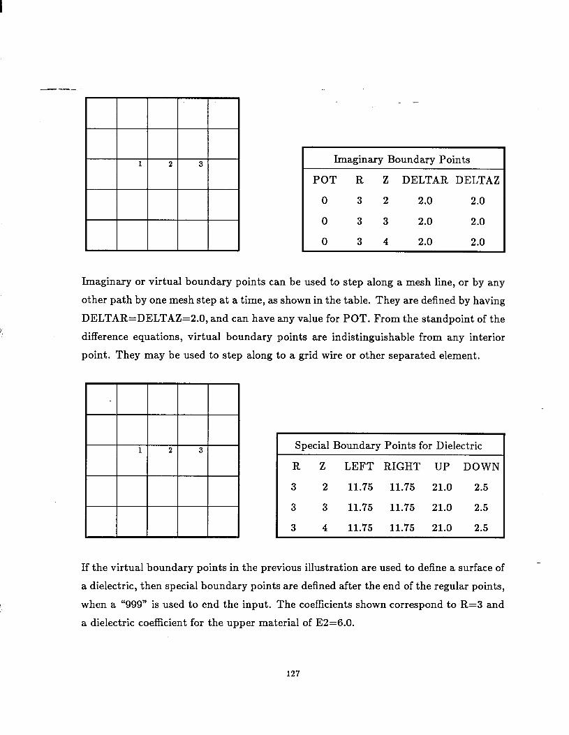
I Imaginary Boundary Points

POT R Z DELTAR DELTAZ

0 3 2 2.0 2.0

0 3 3 2.0 2.0

0 3 4 2.0 2.0

Imaginary or virtual boundary points can be used to step along a mesh line, or by any

other path by one mesh step at a time, as shown in the table. They are defined by having

DELTAR=DELTAZ=2.0, and can have any value for POT. From the standpoint of the

difference equations, virtual boundary points are indistinguishable from any interior

point. They may be used to step along to a grid wire or other separated element.

1 2 3 I Special Boundary Points for Dielectric I R Z LEFT RIGHT UP DOWN

3 2 11.75 11.75 21.0 2.5

3 3 11.75 11.75 21.0 2.5

3 4 11.75 11.75 21.0 2.5

If the virtual boundary points in the previous illustration are used to define a surface of

a dielectric, then special boundary points are defined after the end of the regular points,

when a “999” is used to end the input. The coefficients shown correspond to R=3 and

a dielectric coefficient for the upper material of E2=6.0.

127

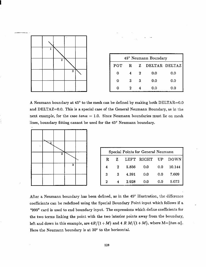
I

I- ~~~~ 45’ Neumann Boundary

POT R Z DELTAR DELTAZ

0 4 2 0.0 0.0

0 3 3 0.0 0.0

0 2 4 0.0 0.0

A Neumann boundary at 45’ to the mesh can be defined by making both DELTAR=O.O

and DELTAZ=O.O. This is a special case of the General Neumann Boundary, as in the

next example, for the case tuna = 1.0. Since Neumann boundaries must lie on mesh

lines, boundary fitting cannot be used for the 45’ Neumann boundary.

Special Points for General Neumann I

R Z LEFT RIGHT UP DOWN

4 2 5.856 0.0 0.0 10.144

3 3 4.391 0.0 0.0 7.609

2 4 2.928 0.0 0.0 5.072

After a Neumann boundary has been defined, as in the 45’ illustration, the difference

coefficients can be redefined using the Special Boundary Point input which follows if a

“999” card is used to end boundary input. The expressions which define coefficients for

the two terms linking the point with the two interior points away from the boundary,

left and down in this example, are 4R/(l+M) and 4 R M/(l+M), where M=(Itan a(/.

Here the Neumann boundary is at 30’ to the horizontal.

128

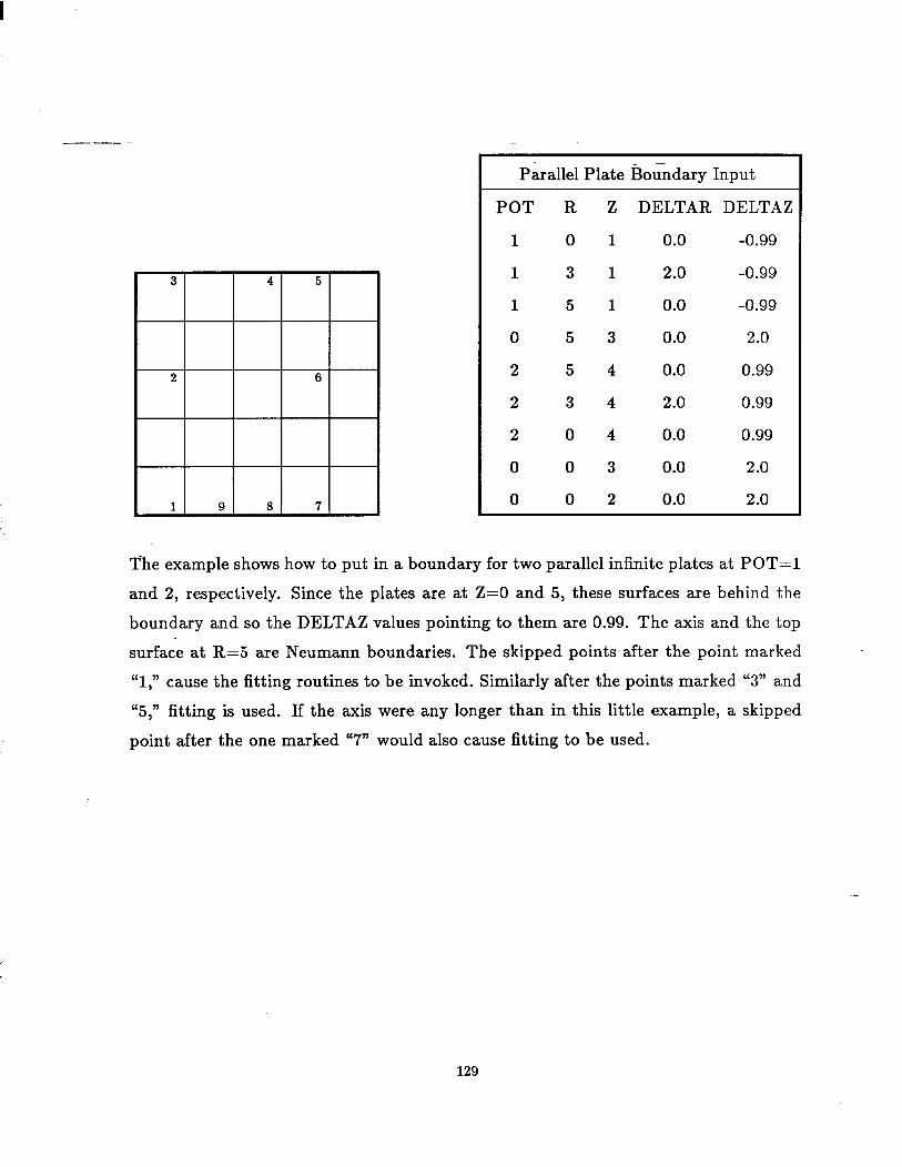
Parallel Plate Boundary Input

POT R Z DELTAR DELTAZ

0 1

3 1

5 1

5 3

5 4

3 4

0 4

0 3

0 2

0.0

2.0

0.0

0.0

0.0

2.0

0.0

0.0

0.0

-0.99

-0.99

-0.99

2.0

0.99

0.99

0.99

2.0

2.0

The example shows how to put in a boundary for two parallel infinite plates at POT=1

and 2, respectively. Since the plates are at Z=O and 5, these surfaces are behind the

boundary and so the DELTAZ values pointing to them are 0.99. The axis and the top

surface at R=5 are Neumann boundaries. The skipped points after the point marked

“1,” cause the fitting routines to be invoked. Similarly after the points marked “3” and

“5,” fitting is used. If the axis were any longer than in this little example, a skipped

point after the one marked “7” would also cause fitting to be used.

129