Efficiently decoding Reed-Muller codes from random errors∗

Ramprasad Saptharishi† Amir Shpilka‡ Ben Lee Volk∗

Abstract

Reed-Muller codes encode an m-variate polynomial of degree r by evaluating it on all pointsin 0, 1m. We denote this code by RM(m, r). The minimum distance of RM(m, r) is 2m−r andso it cannot correct more than half that number of errors in the worst case. For random errorsone may hope for a better result.

In this work we give an efficient algorithm (in the block length n = 2m) for decoding ran-dom errors in Reed-Muller codes far beyond the minimum distance. Specifically, for low ratecodes (of degree r = o(

√m)) we can correct a random set of (1/2− o(1))n errors with high

probability. For high rate codes (of degree m− r for r = o(√

m/ log m)), we can correct roughlymr/2 errors.

More generally, for any integer r, our algorithm can correct any error pattern in RM(m, m−(2r + 2)) for which the same erasure pattern can be corrected in RM(m, m − (r + 1)). Theresults above are obtained by applying recent results of Abbe, Shpilka and Wigderson (STOC,2015), and Kudekar et al. (STOC, 2016) regarding the ability of Reed-Muller codes to correctrandom erasures.

The algorithm is based on solving a carefully defined set of linear equations and thus it issignificantly different than other algorithms for decoding Reed-Muller codes that are based onthe recursive structure of the code. It can be seen as a more explicit proof of a result of Abbe etal. that shows a reduction from correcting erasures to correcting errors, and it also bares somesimilarities with the famous Berlekamp-Welch algorithm for decoding Reed-Solomon codes.

∗A preliminary version of this paper has been accepted for publication in Proceedings of the 48th Annual ACMSymposium on Theory of Computing (STOC 2016)†Department of Computer Science, Tel Aviv University, Tel Aviv, Israel, E-mails: ramprasad@cmi.ac.in,

benleevolk@gmail.com. The research leading to these results has received funding from the European Community’sSeventh Framework Programme (FP7/2007-2013) under grant agreement number 257575.‡Department of Computer Science, Tel Aviv University, Tel Aviv, Israel, shpilka@post.tau.ac.il. The research

leading to these results has received funding from the European Community’s Seventh Framework Programme(FP7/2007-2013) under grant agreement number 257575.

1 Introduction

Consider the following challenge:

Given the truth table of a polynomial f (x) ∈ F2[x1, . . . , xm] of degree at most r, inwhich 1/2− o(1) fraction of the locations were flipped (that is, given the evaluationsof f over Fm

2 with nearly half the entries corrupted), recover f efficiently.

If the errors are adversarial, then clearly this task is impossible for any degree bound r ≥ 1: anytwo different linear polynomials disagree on half of the domain, so f cannot be recovered evenif an adversary flips a quarter of the bits. Hence, we turn to considering random sets of errorsof size (1/2 − o(1))2m, and we hope to recover f with high probability (in this case, one mayalso consider the setting where each bit is independently flipped with probability 1/2− o(1). Bystandard Chernoff bounds, both settings are almost equivalent).

Even in the random model, if every bit was flipped with probability exactly 1/2, the situation isagain hopeless: in this case the input is completely random and carries no information whatsoeverabout the original polynomial.

It turns out, however, that even a very small relaxation leads to a dramatic improvement inour ability to recover the hidden polynomial: in this paper we prove, among other results, thateven at corruption rate 1/2− o(1) and degree bound as large as o(

√m), we can efficiently recover

the unique polynomial f whose evaluations were corrupted. Note that in the worst case, given apolynomial of such a high degree, an adversary can flip a tiny fraction of the bits — just slightlymore than 1/2

√m — and prevent unique recovery of f , even if we do not require an efficient

solution; and yet, in the average case, we can deal with flipping almost half the bits.Recasting the playful scenario above in a more traditional terminology, this paper deals with

similar questions related to recovery of low-degree multivariate polynomials from their randomlycorrupted evaluations on Fm

2 , or in the language of coding theory, we study the problem of decod-ing Reed-Muller codes under random errors in the binary symmetric channel (BSC). We turn to somebackground and motivation.

1.1 Reed-Muller Codes

Reed-Muller (RM) codes were introduced in 1954, first by Muller [Mul54] and shortly after byReed [Ree54] who also provided a decoding algorithm. They are among the oldest and simplestcodes to construct — the codewords are multivariate polynomials of a given degree, and the en-coding function is just their evaluation vectors. In this work we mainly focus on the most basiccase where the underlying field is F = F2, the field of two elements, although our techniques dogeneralize to larger finite fields. Over F2, the Reed-Muller code of degree r in m variables, denotedby RM(m, r), has block length n = 2m, rate ( m

≤r)/2m and its minimum distance is 2m−r.

1

RM codes have been extensively studied with respect to decoding errors in both the worst caseand random setting. We begin by giving a review of Reed-Muller codes and their use in theoreticalcomputer science and then discuss our results.

Background

Error-correcting codes (over both large and small finite fields) have been extremely influentialin the theory of computation, playing a central role in some important developments in severalareas such as cryptography (e.g. [Sha79] and [BF90]), theory of pseudorandomness (e.g. [BV10]),probabilistic proof systems (e.g. [BFL91, Sha92] and [ALM+98]) and many more.

An important aspect of error correcting codes that received a lot of attention is designing effi-cient decoding algorithms. The objective is to come up with an algorithm that can correct a certainamounts of errors in a received word. There are two settings in which this problem is studied:

Worst case errors: This is also referred to as errors in the Hamming model [Ham50]. Here, thealgorithm should recover the original message regardless of the error pattern, as long as thereare not too many errors. The number of errors such a decoding algorithm can tolerate is upperbounded in terms of the distance of the code. The distance of the code C is the minimum Hammingdistance of any two codewords in C. If the distance is d, then one can uniquely recover from at mostd− 1 erasures and from b(d− 1)/2c errors. For this model of worst-case errors it is easy to provethat Reed-Muller codes perform badly. They have relatively small distance compared to whatrandom codes of the same rate can achieve (and also compared to explicit families of codes).

Another line of work in Hamming’s worst case setting concerns designing algorithms that cancorrect beyond the unique-decoding bound. Here there is no unique answer and so the algorithmreturns a list of candidate codewords. In this case the number of errors that the algorithm can tol-erate is a parameter of the distance of the code. This question received a lot of attention and amongthe works in this area we mention the seminal works of Goldreich and Levin on Hadamard Codes[GL89] and of Sudan [Sud97] and Guruswami and Sudan [GS99] on list decoding Reed-Solomoncodes. Recently, the list-decoding question for Reed-Muller codes was studied by Gopalan, Kli-vans and Zuckerman [GKZ08] and by Bhowmick and Lovett [BL15], who proved that the listdecoding radius1 of Reed-Muller codes, over F2, is at least twice the minimum distance (recallthat the unique decoding radius is half that quantity) and is smaller than four times the minimumdistance, when the degree of the code is constant.

Random errors: A different setting in which decoding algorithms are studied is Shannon’smodel of random errors [Sha48]. In Shannon’s average-case setting (which we study here), acodeword is subjected to a random corruption, from which recovery should be possible with highprobability. This random corruption model is called a channel. The two most basic ones, the Binary

1The maximum distance η for which the number of code words within distance η is only polynomially large (in n).

2

Erasure Channel (BEC) and the Binary Symmetric Channel (BSC), have a parameter p (which maydepend on n), and corrupt a message by independently replacing, with probability p, the symbolin each coordinate, with a “lost” symbol in the BEC(p) channel, and with the complementarysymbol in the BSC(p) case. In his paper Shannon studied the optimal trade-off achievable forthese channels (and many other channels) between the distance and rate. For every p, the capacityof BEC(p) is 1− p, and the capacity of BSC(p) is 1− h(p), where h is the binary entropy function.2

Shannon also proved that random codes achieve this optimal behavior. That is, for every 0 < ε

there exist codes of rate 1− h(p)− ε for the BSC (and rate 1− p− ε for the BEC), that can decodefrom a fraction p of errors (erasures) with high probability.

For our purposes, it is more convenient to assume that the codeword is subjected to a fixednumber s of random errors. Note that by the Chernoff-Hoeffding bound, (see e.g., [AS92]), theprobability that more than pn + ω(

√pn) errors occur in BSC(p) (or BEC(p)) is o(1), and so we

can restrict ourselves to the case of a fixed number s of random errors, by setting the corruptionprobability to be p = s/n. We refer to [ASW15] for further discussion on this subject.

Decoding erasures to decoding errors

Recently, there has been a considerable progress in our understanding of the behavior of Reed-Muller codes under random erasures. In [ASW15], Abbe, Shpilka and Wigderson showed thatReed-Muller codes achieve capacity for the BEC for both sufficiently low and sufficiently highrates. Specifically, they showed that RM(m, r) achieves capacity for the BEC for r = o(m) orr > m− o(

√m/ log m). More recently, Kudekar et al. [KKM+16] showed that Reed-Muller codes

achieve capacity for the BEC in the entire constant rate regime, that is r ∈ [m/2−O(√

m), m/2 +O(√

m)]. These regimes are pictorially represented in Figure 1.

m/20 m

o(m) o(√(m/ log m))O(

√m)

Figure 1: Regime of r for which RM(m, r) is known to achieve capacity for the BEC

Another result proved by Abbe et al. [ASW15] is that Reed-Muller codes RM(m, m− 2r − 2)can correct any error pattern if the same erasure pattern can be decoded in RM(m, m− r− 1). Thisreduction is appealing on its own, since it connects decoding from erasures — which is easier inboth an intuitive and an algorithmic manner — with decoding from errors; but its importance isfurther emphasized by the progress made later by Kudekar et al., who showed that Reed-Mullercodes can correct many erasures in the constant rate regime, right up to the channel capacity.

2h(p) = −p log2(p)− (1− p) log2(1− p), for p ∈ (0, 1), and h(0) = h(1) = 0.

3

This result show that RM(m, m− (2r + 2)) can cope with most error patterns of weight (1−o(1))( m

≤r), which is the capacity of RM(m, m − (r + 1)) for the BEC. While this is polynomiallysmaller than what can be achieved in the Shannon model of errors for random codes of the samerate, this number is still much larger (super-polynomial) than the distance (and the list-decodingradius) of the code, which is 22r+2. Also, since RM

(m, m

2 + o(√

m))

can cope with( 1

2 − o(1))-

fraction of erasures, this translation implies that RM(m, o(√

m)) can handle that many randomerrors.

However, a shortcoming of the proof of Abbe et al. for the BSC is that it is existential. Inparticular it does not provide an efficient decoding algorithm. Thus, Abbe et al. left open thequestion of coming up with a decoding algorithm for Reed-Muller codes from random errors.

1.2 Our contributions

In this work we give an efficient decoding algorithm for Reed-Muller codes that matches the pa-rameters given by Abbe et al. Following the aforementioned results about the erasure correctingability of Reed-Muller codes, the results can be partitioned into the low-rate and the high-rateregimes. We begin with the result for the low rate case.

Theorem 1 (Low rate, informal). Let r < δ√

m for a small enough δ. Then, there is an efficient algorithmthat can decode RM(m, r) from a random set of (1− o(1)) · ( m

≤(m−r)/2) errors. In particular, if r = o(√

m),the algorithm can decode from

( 12 − o(1)

)· 2m errors. The running time of the algorithm is O(n4) and it

can be simulated in NC.

For high rate Reed-Muller codes, we cannot hope to achieve such a high error correction capa-bility as in the low rate case, even information theoretically. We do give, however, an algorithmthat corrects many more errors (a super-polynomially larger number) than what the minimumdistance of the code suggests, and its running time is also nearly linear in the block length of thecode.

Theorem 2 (High rate, informal). Let r = o(√

m/ log m). Then, there is an efficient algorithm that candecode RM(m, m− (2r + 2)) from a random set of (1− o(1))( m

≤r) errors. Moreover, the running time ofthe algorithm is 2m · poly(( m

≤r)) and it can be simulated in NC.

Recall that the block length of the code is n = 2m, and thus the running time is near linear in nwhen r = o(m).

A general property of our algorithm is that it corrects any error pattern in RM(m, m− 2r− 2)for which the same erasure pattern in RM(m, m− r− 1) can be corrected. Stated differently, if anerasure pattern can be corrected in RM(m, m− r− 1) then the same pattern, where the “lost” sym-bol is replaced with arbitrary 0/1 values, can be corrected in RM(m, m− (2r + 2)). This propertyis useful when we know RM(m, m− r− 1) can correct a large set of erasures with high probabil-ity, that is, when m− r− 1 falls in the red region in Figure 1. Thus, our result has implications also

4

beyond the above two instances. In particular, it may be the case that our algorithm performs wellfor other rates as well. For example, consider the following question and the theorem it implies.

Question 3. Does RM(m, m− r− 1) achieve capacity for the BEC?

Theorem 4 (informal). For any value r for which the answer to Question 3 is positive, there exists anefficient algorithm that decodes RM(m, m − 2r − 2) from a random set of (1 − o(1))( m

≤r) errors withprobability (1 − o(1)) (over the random errors). Moreover, the running time of the algorithm is 2m ·poly

(( m≤r))

.

Recall that Abbe et al. [ASW15] also proved that the answer to Question 3 is positive forr = m − o(m) (that is, for RM(m, o(m))) but this case does not help us as we need to considerRM(m, m − (2r + 2)) and m − (2r + 2) < 0 in this case. The coding theory community seemsto believe the answer to Question 3 is positive, for all values of r, and conjectures to that effectwere made3 in [CF07, Arı08, MHU14]. Recent simulations have also suggested that the answerto the question is positive [Arı08, MHU14]. Thus, it seems natural to believe that the answeris positive for most values of r, even for r = Θ(m). As a conclusion, the belief in the codingtheory community suggests that our algorithm can decode a random set of roughly ( m

≤r) errorsin RM(m, m − (2r + 2)). For example, for r = ρ · m, where ρ < 1/2, the minimum distance ofRM(m, m− (2r + 2)) is roughly 22ρm whereas our algorithm can decode from roughly 2h(ρ)m ran-dom errors (assuming the answer to Question 3 is positive), which is a much larger quantity forevery ρ < 1/2.

In Section 3, we also present an abstraction of our decoding procedure that may be applicableto other linear codes. This is a generalization of the abstract Berlekamp-Welch decoder or “error-locating pairs” method of Duursma and Kotter [DK94] that connects decodable erasure patternson a larger code to decodable error patterns. A specific instantiation of this was observed byAbbe et al. [ASW15] by connecting decodable error patterns of any linear code C to decodableerasure patterns of an appropriate “tensor” C′ of C (by essentially embedding these codes in alarge enough RM code). Although Abbe et al. did not provide an efficient decoding algorithm,the algorithm we present directly applies here (Section 3.2). The abstraction of the “error-locatingpairs” method presented in Section 3 should hopefully be applicable in other contexts too, espe-cially considering the generality of the results of [KKM+16].

1.3 Related literature

In Section 1.1 we surveyed the known results regarding the ability of Reed-Muller codes to correctrandom erasures. In this section we summarize the results known about recovering RM codesfrom random errors.

3The belief that RM codes achieve capacity is much older, but we did not trace back where it appears first.

5

Once again, it is useful to distinguish between the low rate and the high rate regime of Reed-Muller codes. We shall use d to denote the distance of the code in context. For RM(m, r) codes,d = 2m−r.

In [Kri70], the majority logic algorithm of [Ree54] is shown to succeed in recovering all buta vanishing fraction of error patterns of weight up to d log d/4 for all RM codes of positive rate.In [Dum06], Dumer showed for all r such that min(r, m− r) = ω(log m) that most error patternsof weight at most (d log d/2) · (1 − log m

log d ) can be recovered in RM(m, r). To make sense of theparameters, we note that when r = m− ω(log m) the weight is roughly (d log d/2). To comparethis result to ours, we first consider the case when r = m− o(

√m/ log m). Here the algorithm of

[Dum06] can correct roughly 2o(√

m/ log m) random errors in RM(m, r) whereas Theorem 2 gives analgorithm for correcting roughly mo(

√m/ log m) ≈ (d log d)O(log m) random errors.

Let us now consider the case r = ρm for some constant 0 < ρ < 1. Here, the minimum distanceis 2(1−ρ)m. In this regime, the bound in the above result of [Dum06] is equal to O(d log d). On theother hand, assuming a positive answer to Question 3, Theorem 4 implies an efficient decodingalgorithm for RM(m, ρm) that can decode from, roughly, ( m

≤ 1−ρ2 m) ≈ 2h( 1−ρ

2 )m random errors, whereagain h is the binary entropy function.

When ρ is a small constant, we have that h( 1

2 −ρ2

)≈ 1−Θ(ρ2), so the number of errors we can

correct is roughly 2(1−Θ(ρ2))m, which is a larger quantity than the minimum distance d = 2(1−ρ)m,and also than the above O(d log d) result of [Dum06].

When ρ = 1− ε for some small constant ε > 0, h(ε/2) = Ω(ε log(1/ε)), and the number oferrors we can correct is around 2ε log(1/ε)m ≈ dlog(1/ε).

As a last example, suppose ρ = 1/2− δ for some small constant δ > 0. In this case,

h(

1− ρ

2

)= h(1/4 + δ/2) = h(1/4) + Θ(δ) =

12+

34

log(4/3) + Θ(δ),

which gives a bound of roughly 2(1/2+η+δ)m on the number of errors, for an absolute constantη > 0, compared to 2(1/2+δ)m, which is the minimum distance.

In order to exhibit the fact that h( 1

2 −ρ2

)is always larger than 1 − ρ, we plot the graphs of

the two functions side by side in Figure 2. Recall that the former function is the logarithm of thenumber of errors we can correct, normalized by m, assuming a positive answer to Question 3; andthe latter is the logarithm of the minimum distance, normalized by m.

We now turn to considering RM codes of low rate. For the special case of r = 1, 2, [HKL05]shows that RM(m, r) codes are capacity-achieving. In [SP92], it is shown that RM codes of fixedorder (i.e., r = O(1)) can decode most error patterns of weight up to 1

2 n(1−√

c(2r − 1)mr/nr!),where c > ln(4). In [ASW15], Abbe et al. settled the question for low order Reed-Muller codesproving that RM(m, r) codes achieve capacity for the BSC when r = o(m) [ASW15]. We notehowever that all the results mentioned here are existential in nature and do not provide an efficient

6

0 0.2 0.4 0.6 0.8 10

0.2

0.4

0.6

0.8

1

ρ = r/m, relative degree of RM(m, r)

num

ber

ofer

rors

corr

ecte

d

1− ρ

h(

1−ρ2

)

Figure 2: The number of correctable errors as a function of the degree, in logarithmic scale, normalized by m. The redline corresponds to the algorithm given in [Dum06], which corrects ≈ d log d ≈ 2(1−ρ)m · (1− ρ)m errors. The blue

curve corresponds to the algorithm given in this work, which corrects ≈ 2h( 1−ρ2 )m errors.

decoding algorithm.A line of work by Dumer [Dum04, DS06] based on recursive algorithms (that exploit the recur-

sive structure of Reed-Muller codes), obtains algorithmic results mainly for low-rate regimes. In[Dum04], it is shown that for a fixed degree, i.e., r = O(1), an algorithm of complexity O(n log n)can correct most error patterns of weight up to n(1/2− ε) given that ε exceeds n−1/2r

. In [Dum06],this is improved to errors of weight up to 1

2 n(1 − (4m/d)1/2r) for all r = o(log m). The case

r = ω(log m) is also covered in [Dum06], as described above.We note that all the efficient algorithms mentioned above (both for high- and low-rate) rely

on the so called Plotkin construction of the code, that is, on its recursive structure (expand-ing an m-variate polynomial according to the m-th variable f (x1, . . . , xm) = xmg(x1, . . . , xm−1) +

h(x1, . . . , xm−1)), whereas our approach is very different.We summarize and compare our results with [Dum04, DS06, Dum06] for various range of

parameters in Figure 3 (degree is r and distance is d = 2m−r). The dotted region in Figure 3 corre-sponds to the uncovered region in Figure 1 beyond m/2, via the connection given in Theorem 4.Figure 2 compares our results, for the linear degree regime (r = ρm), with those of [Dum06].

1.4 Notation and terminology

Before explaining the idea behind the proofs of our results we need to introduce some notationand parameters. We shall use the same notation as [ASW15].

• We denote by M(m, r) the set of m-variate monomials over F2 of degree at most r.

7

m/20 m

log m log m

o(√

m)

o(√

m/ log m)

Degree (r) of RM(m, r):

(see also Figure 2)

[Dum04, DS06, Dum06]:≈ n/2 errors O(d log d) = O(2(1−ρ)m · (1− ρ)m) errors for ρ = r/m

O(n log n) time algorithm

Our results:≈ n/2 errors

O(n4) time algo.

(d log d)O(log m) errors

n1+o(1) time algo.

2h(

1−ρ2

)m errors for ρ = r/m

assuming a positive answer to Question 3

Figure 3: Comparison with [Dum04, DS06, Dum06]

• For non-negative integers r ≤ m, RM(m, r) denotes the Reed-Muller code whose codewordsare the evaluation vectors of all multivariate polynomials of degree at most r on m booleanvariables. The maximal degree r is sometimes called the order of the code. The block lengthof the code is n = 2m, the dimension k = k(m, r) = ∑r

i=0 (mi )

def= ( m

≤r), and the distanced = d(m, r) = 2m−r. The code rate is given by R = k(m, r)/n.

• We use E(m, r) to denote the “evaluation matrix” of parameters m, r, whose rows are indexedby all monomials in M(m, r), and whose columns are indexed by all vectors in Fm

2 . The valueat entry (M, u) is equal to M(u). For u ∈ Fm

2 , we denote by ur the column of E(m, r) indexedby u, which is a k-dimensional vector, consisting of all evaluations of degree ≤ r monomialsat u. For a subset of columns U ⊆ Fm

2 we denote by Ur the corresponding submatrix ofE(m, r).

• E(m, r) is a generator matrix for RM(m, r). The duality property of Reed-Muller codes (see,for example, [MS77]) states that E(m, m − r − 1) is a parity-check matrix for RM(m, r), orequivalently, E(m, r) is a parity-check matrix for RM(m, m− r− 1).

• We associate with a subset U ⊆ Fm2 its characteristic vector 1U ∈ Fn

2 . We often think of thevector 1U as denoting either an erasure pattern or an error pattern.

• For a positive integer n, we use the standard notation [n] for the set 1, 2, . . . , n.

We next define what we call the degree-r syndrome of a set.

Definition 5 (Syndrome). Let r ≤ m be two positive integers. The degree-r syndrome, or simply r-syndrome of a set U = u1, . . . , ut ⊆ Fm

2 is the ( m≤r)-dimensional vector α whose entries are indexed by

8

all monomials M ∈M(m, r), such that

αMdef=

t

∑i=1

M(ui).

Note that this is nothing but the syndrome of the error pattern 1U ∈ Fn2 in the code RM(m, m−

r− 1) (whose parity check matrix is the generator matrix of RM(m, r)).

1.5 Proof techniques

In this section we describe our approach for constructing a decoding algorithm. Recall that thealgorithm has the property that is decodes in RM(m, m − 2r − 2) any error pattern U which iscorrectable from erasures in RM(m, m− r − 1). Such patterns are characterized by the propertythat the columns of E(m, r) corresponding to the elements of U are linearly independent vectors.Thus, it suffices to give an algorithm that succeeds whenever the error pattern 1U gives rise tosuch linearly independent columns, which happens with probability 1− o(1) for the regime ofparameters mentioned in Theorem 1 and Theorem 2.

So let us assume from now on that the error pattern 1U corresponds to a set of linearly indepen-dent columns in E(m, r). Notice that by the choice of our parameters, our task is to recover U fromthe degree (2r + 1)-syndrome of U. Furthermore, we want to do so efficiently. For convenience,let t = |U| = (1− o(1))( m

≤r).Recall that the degree-(2r + 1) syndrome of U is the ( m

≤2r+1)-long vector α such that for everymonomial M ∈ M(m, 2r + 1), αM = ∑t

i=1 M(ui). Imagine now that we could somehow finddegree-r polynomials fi(x1, . . . , xm) satisfying fi(uj) = δi,j. Then, from knowledge of α and, say,f1, we could compute the following sums:

σ` =t

∑i=1

( f1 · x`)(ui), ` ∈ [m].

Indeed, if we know α and f1 then we can compute each σ`, as it just involves summing severalcoordinates of α (since deg( f1 · x`) ≤ r + 1). We now observe that

σ` =t

∑i=1

( f1 · x`)(ui) = ( f1 · x`)(u1) = (u1)`.

In other words, knowledge of such an f1 would allow us to discover all coordinates of u1 and inparticular, we will be able to deduce u1, and similarly all other ui using fi.

Our approach is thus to find such polynomials fi. What we will do is set up a system of linearequations in the coefficients of an unknown degree r polynomial f and show that f1 is the uniquesolution to the system. Indeed, showing that f1 is a solution is easy and the hard part is proving

9

that it is the unique solution.To explain how we set the system of equations, let us assume for the time being that we actually

know u1. Let f = ∑M∈M(m,r) cM ·M, where we think of cM as unknowns. Consider the followinglinear system:

1.t

∑i=1

f (ui) = f (u1) = 1,

2.t

∑i=1

( f ·M)(ui) = M(u1), for all M ∈M(m, r).

In words, we have a system of 2+ ( m≤r) + m · ( m

≤r) equations in ( m≤r) variables (the coefficients of f ).

Observe that f = f1 is indeed a solution to the system. Furthermore, a solution to the equationsin item 2 gives (the coefficients of) a linear combination of the columns of Ur that equals ur

1. Sincethose columns are linearly independent, there is a unique such linear combination, which impliesf1 is the unique solution to the system.

Now we explain what to do when we do not know u1. Let v = (v1, . . . , vm) ∈ Fm2 . We modify

the linear system above to:

1.t

∑i=1

f (ui) = f (v) = 1,

2.t

∑i=1

( f ·M)(ui) = M(v) for all M ∈M(m, r).

3.t

∑i=1

( f ·M · (x` + v` + 1))(ui) = M(v) for all ` ∈ [m] and M ∈M(m, r).

Now the point is that one can prove that if a solution exists then it must be the case that v is anelement of U. Indeed, the set of equations in item 2 implies that vr is in the linear span of thecolumns of Ur. The linear equations in item 3 then imply that v must actually be in the set U.

An alternate perspective is to interpret the above equations as solving for a degree r polyno-mial f such that

t

∑i=1

( f · g)(ui) = g(v) for all g of degree at most r + 1.

If v = u1, then as mentioned earlier we have a polynomial f such that f (u1) = 1 and f (ui) = 0for all i = 2, . . . , t so we clearly have a solution for f .

On the other hand, if v /∈ U then we can show (Lemma 13) that there is a polynomial g ofdegree at most r + 1 such that g(ui) = 0 for all i ∈ [t] but g(v) = 1. This clearly implies that theabove system cannot have a solution as ∑( f · g)(ui) = 0 and g(v) = 1.

Notice that what we actually do amounts to setting, for every v ∈ Fm2 , a system of linear

equations of size roughly ( m≤r). Such a system can be solved in time poly

(( m≤r))

. Thus, when we

go over all v ∈ Fm2 we get a running time of 2m · poly

(( m≤r))

, as claimed.

10

Our proof can be viewed as an algorithmic version of the proof of Theorem 1.8 of Abbe et al.[ASW15]. That theorem asserts that when the columns of Ur are linearly independent, the (2r+ 1)-syndrome of U is unique. In their proof of the theorem they first use the (2r)-syndrome to claimthat if V is another set with the same (2r)-syndrome then the column span of Ur is the same as thatof Vr. Then, using the degree (2r + 1) monomials they deduce that U = V. This is similar to whatour linear system does, but, in contrast, [ASW15] did not have an efficient algorithmic version ofthis statement.

2 Decoding Algorithm For Reed-Muller Codes

We begin with the following basic linear algebraic fact.

Lemma 6. Let u1, . . . , ut ∈ Fm2 such that ur

1, . . . , urt are linearly independent. Then, for every i ∈ [t],

there exists a polynomial fi so that for every j ∈ [t],

fi(uj) = δi,j =

1 if i = j

0 otherwise.

For completeness, we give the short proof.

Proof. Consider the matrix Ur ∈ Ft×( m

≤r)

2 whose i-th row is uri . A polynomial fi which satisfies

the properties of the lemma is a solution to the linear system Urx = ei, where ei ∈ Ft2 is the i-th

elementary basis vector (that is, (ei)j = δi,j), and the ( m≤r) unknowns are the coefficients of fi. By

the assumption that U is of full rank, indeed there exists a solution.

The algorithm would proceed by making a guess v = (v1, . . . , vm) ∈ Fm2 for one of the error

locations. If we could come up with an efficient way to verify that the guess is correct, this wouldimmediately yield a decoding algorithm. We shall verify our guess by using the dual polynomialsf1, . . . , ft described above. We shall find them by solving a system of linear equations that can beconstructed from the (2r + 1)-syndrome of u1, . . . , um. We will need the following crucial, yetsimple, observation.

Observation 7. Let f be any m-variate polynomial of degree at most 2r + 1, and u1, . . . , ut ∈ Fm2 . Then,

the sum ∑ti=1 f (ui) can be computed given the (2r + 1)-syndrome of u1, . . . , ut, in time O

(( m

2r+1)).

Proof. For any M ∈ M(m, 2r + 1), denote αM = ∑ti=1 M(ui) (so that α = (αM)M∈M(M,2r+1) is

11

precisely the syndrome of u1, . . . , ut). Write f = ∑M∈M(m,2r+1) cM ·M, where cM ∈ F2, then

t

∑i=1

f (ui) =t

∑i=1

∑M∈M(m,2r+1)

cM ·M(ui)

= ∑M∈M(m,2r+1)

cM

(t

∑i=1

M(ui)

)= ∑

M∈M(m,2r+1)cMαM.

The following lemma shows how to verify a guess for an error location. It is the main ingre-dient in the analysis of our algorithm and the reason why it works. Basically, the lemma givesa system of linear equations whose solution enables us to decide whether a given v ∈ Fm

2 is acorrupted coordinate or not, without knowledge of the set of errors U but only of its syndrome.In a sense, this lemma is analogous to the Berlekamp-Welch algorithm, which also gives a systemof linear equations whose solution reveals the set of erroneous locations ([WB86], and see also theexposition in Chapter 13 of [GRS14]).

Lemma 8 (Main Lemma). Let u1, . . . , ut ∈ Fm2 such that ur

1, . . . , urt are linearly independent, and v =

(v1, . . . , vm) ∈ Fm2 . Suppose there exists a multilinear polynomial f ∈ F2[x1, . . . , xm] with deg( f ) ≤ r

such that for every monomial M ∈M(m, r),

1.t

∑i=1

f (ui) = f (v) = 1,

2.t

∑i=1

( f ·M)(ui) = M(v), and

3.t

∑i=1

( f ·M · (x` + v` + 1))(ui) = M(v) for every ` ∈ [m].

Then there exists i ∈ [t] such that v = ui.

Observe that if indeed v = ui for some i ∈ [t], then the polynomial fi guaranteed by Lemma 6satisfies those equations. Hence, the lemma should be interpreted as saying the converse: thatif there exists such a solution, then v = ui for some i. Further, given the (2r + 1)-syndrome ofu1, . . . , ut as input, Observation 7 shows that each of the above constraints are linear constraintsin the coefficients of f . Thus, finding such an f is merely solving a system of O

(( m≤r))

linear

equations in ( m≤r) unknowns and can be done in poly

(( m≤r))

time.

Proof of Lemma 8. Let J =

j | f (uj) = 1

. Note that by item 1 it holds that J 6= ∅.

Subclaim 9. ∑i∈J

uri = vr.

12

Proof. Let M ∈ M(m, r). We show that ∑i∈J M(ui) = M(v), i.e., that the Mthcoordinate of ∑i∈J ur

i is equal to that of vr. Indeed, as f satisfies the constraints initem 2,

M(v) =t

∑i=1

( f ·M)(ui) = ∑i∈J

( f ·M)(ui) + ∑i 6∈J

( f ·M)(ui) = ∑i∈J

M(ui). (Subclaim)

For any ` ∈ [m], let J` =

j | f (uj) = 1 and (uj)` = v`⊆ J. Observe that this definition implies

that for every j ∈ [t], the index j is in J` if and only if ( f · (x` + v` + 1))(uj) = 1. Using a similarargument, we can show the following.

Subclaim 10. For every ` ∈ [m],

∑i∈J`

uri = vr. (11)

Proof. Again, for any M ∈M(m, r) the constraints in item 3 imply that

M(v) =t

∑i=1

( f ·M · (x` + v` + 1))(ui) = ∑i∈J`

M(ui). (Subclaim)

From the above claims,vr = ∑

i∈Jur

i = ∑i∈J1

uri = · · · = ∑

i∈Jm

uri .

By the linear independence of ur1, . . . , ur

t, it follows that J = J1 = J2 = · · · = Jm. Indeed, thereis a unique linear combination of ur

1, . . . , urt that gives vr. The only vector which can be in the

(non-empty) intersection⋂m

k=1 Jk is v, and so there exists i ∈ [t] so that ui = v.

As mentioned in Section 1.5, an alternate perspective to view the set of equations as solvingfor a degree r polynomial f such that

t

∑i=1

( f · g)(ui) = g(v) for every polynomial g of degree at most r + 1. (12)

The following lemma is a slightly different way4 to prove Lemma 8.

Lemma 13. If v /∈ U , then there exists a polynomial g of degree at most r + 1 such that g(v) = 1 andg(u) = 0 for all u ∈ U .

Proof. From Lemma 6, for each i ∈ [t] we have a polynomial fi such that fi(ui) = 1 and fi(uj) = 0for all j ∈ [t] \ i.

4This alternate perspective was suggested by an anonymous reviewer.

13

Case 1: fi(v) = 1 for some i ∈ [t].Since v 6= ui, there is some coordinate ` ∈ [m] such that v` 6= ui`. Then g = fi · (x − ui`) is a

polynomial that is zero in U but non-zero on v. Since fi has degree at most r, the polynomial g hasdegree at most r + 1.

Case 2: fi(v) = 0 for all i ∈ [t].In this case we can take g = 1− ∑t

i=1 fi as g(ui) = 0 for all i ∈ [t] and g(v) = 1. Also, g hasdegree at most r.

Lemma 8 implies a natural algorithm for decoding from t errors indexed by vectorsu1, . . . , ut, assuming ur

1, . . . , urt are linearly independent, that we write down explicitly in

Algorithm 1.

Algorithm 1 : Reed-Muller Decoding

Input: A (2r + 1)-syndrome of u1, . . . , ut1: E = ∅2: for all v = (v1, . . . , vm) ∈ Fm

2 do3: Solve for a polynomial f ∈ F2[x1, . . . , xm] of degree at most r that satisfies

t

∑i=1

( f ·M)(ui) = M(v) for all M ∈M(m, r + 1).

4: if there is a polynomial f that satisfies the above system of equations then5: Add v to the set E .6: return the set E as the error locations.

Theorem 14. Given the (2r + 1)-syndrome of t unknown vectors u1, . . . , ut ⊆ Fm2 such that

ur1, . . . , ur

t are linearly independent, Algorithm 1 outputs u1, . . . , ut, runs in time 2m · poly(( m≤r))

and can be realized using a circuit of depth poly(m) = poly(log n).

Proof. The algorithm enumerates all vectors in Fm2 , and for each candidate v checks whether there

exists a solution to the linear system of poly(( m≤r)) equations in poly(( m

≤r)) unknowns given inLemma 8. Observation 7 shows that this system of linear equations can be constructed from the(2r + 1)-syndrome in poly(( m

≤r)) time.By Lemma 6 and Lemma 8, a solution to this system exists if and only if there is i ∈ [t] so that

v = ui. The bound on the running time follows from the description of the algorithm. Further-more, all 2m = n linear systems can be solved in parallel, and each linear system can be solvedwith an NC2 circuit (see, e.g., [MV97]).

Observe that the the proof of correctness for Algorithm 1 is valid, for any value of r, wheneverthe set of error locations u1, . . . , ut satisfies the property that ur

1, . . . , urt are linearly indepen-

14

dent. Therefore, we would like to apply Theorem 14 in settings where ur1, . . . , ur

t are linearlyindependent with high probability.

For the constant rate regime, Kudekar et al. [KKM+16] proved that RM(m, m− r− 1) achievescapacity for r = m/2±O(

√m).

Theorem 15 ([KKM+16]). Let r ≤ m be integers such that r = m/2±O(√

m). Then, for t = (1−o(1))( m

≤r), with probability 1− o(1), for a set of vectors u1, . . . , ut ⊆ Fm2 chosen uniformly at random,

it holds that ur1, . . . , ur

t are linearly independent over F( m≤r)

2 .

Letting r = m/2− o(√

m) and looking at the code RM(m, m − 2r − 2) = RM(m, o(√

m)) sothat ( m

≤r) = (1/2− o(1))2m, we get the following statement, stated earlier as Theorem 1.

Corollary 16. There exists a (deterministic) algorithm that is able to correct t = (1/2− o(1))2m random

errors in RM(m, o(√

m) with probability 1− o(1). The algorithm runs in time 2m ·(( m

m/2−o(√

m))3≤ n4.

Alternatively, we can pick r = m/2 − O(√

m) and correct c · 2m random errors in the codeRM(m, O(

√m)), where c is some positive constant that goes to zero as the constant hidden under

the big O increases.For the high-rate regime, recall the following capacity achieving result proved in [ASW15]:

Theorem 17 ([ASW15], Theorem 4.5). Let ε > 0, r ≤ m be two positive integers and t <

(m−log(( m

≤r))−log(1/ε)≤r ). Then, with probability at least 1− ε, for a set of vectors u1, . . . , ut ⊆ Fm

2 cho-

sen uniformly at random, it holds that ur1, . . . , ur

t are linearly independent over F( m≤r)

2 .

Using Theorem 17, we apply Theorem 14 to obtain the following corollary, which was statedinformally as Theorem 2.

Corollary 18. Let ε > 0, and r ≤ m be two positive integers. Then there exists a (deterministic) algo-rithm that is able to correct t =

⌊(

m−log(( m≤r))−log(1/ε)≤r )

⌋− 1 random errors in RM(m, m− (2r + 2)) with

probability at least 1− ε. The algorithm runs in time 2m · poly(( m≤r))

.

If r = o(√

m/ log m), the bound on t is (1− o(1))( m≤r), as promised.

More generally, a positive answer to Question 3 is equivalent to ur1, . . . , ur

t for t = (1 −o(1))( m

≤r) being linearly independent with probability 1− o(1) (see Corollary 2.9 in [ASW15]), andthus we also obtain the following corollary, which was stated informally as Theorem 4.

Corollary 19. Let r ≤ m be two positive integers. Suppose that RM(m, m− r− 1) achieves capacity forthe BEC. Then there exists a (deterministic) algorithm that is able to correct (1− o(1))( m

≤r) random errors

in RM(m, m− (2r + 2)) with probability 1− o(1). The algorithm runs in time 2m · poly(( m≤r))

.

We note that for all values of r, 2m · poly(( m≤r))

is polynomial in the block length n = 2m, and

when r = o(m) this is equal to n1+o(1).

15

3 Abstractions and Generalizations

3.1 An abstract view of the decoding algorithm

In this section we present a more abstract view of Algorithm 1, in the spirit of the works by Pel-likaan, Duursma and Kotter ([Pel92, DK94]) which abstract the Berlekamp-Welch algorithm (seealso the exposition in [Sud01]). Stated in this way, it is also clear that the algorithm works alsoover larger alphabets, so we no longer limit ourselves to dealing with binary alphabets. As shownin [KKM+16], Reed-Muller codes over Fq (sometimes referred to as Generalized Reed-Muller codes)also achieve capacity in the constant rate regime.

We begin by giving the definition of a (pointwise) product of two vectors, and of two codes.

Definition 20. Let u, v ∈ Fnq . Denote by u ∗ v ∈ Fn

q the vector (u1v1, . . . , unvn). For A, B ⊆ Fnq we

similarly define A ∗ B = u ∗ v | u ∈ A, v ∈ B.

Following the footsteps of Algorithm 1, we wish to decode, in a code C, error patterns whichare correctable from erasures in a related code N, through the use of an error-locating code E. Undersome assumptions on C, N and E, we can use a similar proof in order to do this.

Theorem 21. Let E, C, N ⊆ Fnq be codes with the following properties.

1. E ∗ C ⊆ N

2. For any pattern 1U that is correctable from erasures in N, and for any coordinate i 6∈ U there existsa codeword e ∈ E such that ej = 0 for all j ∈ U and ei = 1.

Then there exists an efficient algorithm that corrects in C any pattern 1U , which is correctable from erasuresin N.

To put things in perspective, earlier we set C = RM(m, m− 2r − 2), N = RM(m, m− r − 1)and E = RM(m, r + 1). It is immediate to observe that item 1 holds in this case, and item 2is guaranteed by Lemma 6: Indeed, consider the error pattern U = u1, . . . , ut and the dualpolynomials fit

i=1, and let v 6∈ U be any other coordinate of the code. If there exists j ∈ [t] suchthat f j(v) = 1, we can pick the codeword g = f j · (1 + x` + v`), where ` is some coordinate suchthat v` 6= (uj)`. g has degree at most r + 1 and so it is a codeword in E, and it can be directlyverified that it satisfies the conditions of item 2. If f j(v) = 0 for all j, we can pick g = 1−∑t

i=1 fi.It is also worth pointing out the differences between our approach and the abstract Berlekamp-

Welch decoder of Duursma and Kotter: They similarly set up codes E, C and N such that E ∗ C ⊆N. However, instead of item 2, they require that for any e ∈ E and c ∈ C, if e ∗ c = 0 then e = 0 orc = 0 (or similar requirements regarding the distances of E and C that guarantee this property).This property, as well as the distance properties, do not hold in the case of Reed-Muller codes.

16

Turning back to the proof of Theorem 21, the algorithm and the proof of correctness turn outto be very short to describe in this level of generality. Given a word y ∈ Fn

q , the algorithm wouldsolve the the linear system a ∗ y = b, in unknowns a ∈ E and b ∈ N. Under the hypothesis of thetheorem, we show that common zeros of the possible solutions for a determine exactly the errorlocations. Once the locations of the errors are identified, correcting them is easy: we can replacethe error locations by the symbol ‘?’ and use an algorithm which corrects erasures (this can alwaysbe done efficiently, when unique decoding is possible, as this merely amounts to solving a systemof linear equations). The algorithm is given in Algorithm 2.

Algorithm 2 : Abstract Decoding Algorithm

Input: received word y ∈ Fnq such that y = c + e, with c ∈ C and e is supported on a set U

1: Solve for a ∈ E, b ∈ N, the linear system a ∗ y = b.2: Let a1, . . . , ak be a basis for the solution space of a, and let E denote the common zeros ofai | i ∈ [k].

3: For every j ∈ E , replace yj with ‘?’, to get a new word y′.4: Correct y′ from erasures in C.

Note that in Theorem 21 we assume that the error pattern U is correctable from erasures in N,whereas Algorithm 2 first computes a set of error locations E and then corrects y′ from erasures inC. Thus, the proof of Theorem 21 can be divided into two steps. The first, and the main one, willbe to show that E = U. The second, which is merely an immediate observation, will be to showthat U is also correctable from erasures in C. We begin with the second part:

Lemma 22. Assume the setup of Theorem 21, and let U be any pattern which is correctable from erasuresin N. Then U is also correctable from erasures in C.

Proof. We may assume that U 6= ∅, as otherwise the statement is trivial. Suppose on the contrarythat U is not correctable from erasures in C, that is, there exists a non-zero codeword c ∈ Csupported on U. For any a ∈ E, we have that a ∗ c is a codeword of N which is supported on asubset of U. In order to reach a contradiction, we want to pick a ∈ E so that a ∗ c is a non-zerocodeword of N, which contradicts the assumption that U is correctable from erasures in N.

Pick i ∈ U so that ci 6= 0. Observe that if U is correctable from erasures in N then so is U \ i.By item 2 in Theorem 21 with respect to the set U \ i there exists a ∈ E with ai = 1. Thus, inparticular a ∗ c is non-zero.

We now prove that main part of Theorem 21, that is, that under the assumptions stated in thetheorem, Algorithm 2 correctly decodes (in C) any error pattern that is correctable from erasuresin N.

Proof of Theorem 21. Write y = c + e, so that c ∈ C is the transmitted codeword and e is supportedon the set of error locations U. As noted above, by Lemma 22 it is enough to show that under the

17

assumptions of the theorem (in particular, that U is correctable from erasures in N), the set of errorlocations E computed by Algorithm 2 equals U.

In the following two lemmas, we argue that any solution a for the system vanishes on the errorpoints, and then that for every other index i, there exists a solution whose i-th entry is non-zero(and so there must be a basis element for the solution space whose i-th entry is non-zero).

The following lemma states that every solution a ∈ E to the equation a ∗ y = b vanishes on U,the support of e. In the pointwise product notation, this is equivalent to showing that a ∗ e = 0.

Subclaim 23. For every a ∈ E, b ∈ N such that a ∗ y = b, it holds that a ∗ e = 0.

Proof. Since a ∗ y = b ∈ N (by the assumption) and a ∗ c ∈ N (by item 1),we get that a ∗ e = a ∗ y − a ∗ c is also a codeword in N. Furthermore, a ∗ e isalso supported on U, and since U is an erasure-correctable pattern in N, the onlycodeword that is supported on U is the zero codeword. (Subclaim)

To finish the proof, we show that for any i 6∈ U, there is a solution a to the system of linearequations with ai = 1.

Subclaim 24. For every i 6∈ U there exists a ∈ E, b ∈ N such that a is 0 on U, ai = 1and a ∗ y = b.

Proof. By item 2, since U is correctable from erasures in N, for every i 6∈ U we canpick a ∈ E such that a is 0 on U and ai = 1. Set b = a ∗ y. It remains to be shownthat b is a codeword of N. This follows from the fact that

b = a ∗ c + a ∗ e = a ∗ c,

where the second equality follows from the fact that a is zero on U (the support ofe). Finally, a ∗ c is a codeword of N by item 1. (Subclaim)

These two claims complete the proof of the theorem.

3.2 Decoding of Linear Codes over F2

In [ASW15], it is observed that their results for Reed-Muller codes imply that for every linear codeN, every pattern which is correctable from erasures in N is correctable from errors in what theycall the “degree-three tensoring” of N. Here we remark that this is nothing but a special case ofTheorem 21 with an appropriate setting of the codes E, C, N. We begin by briefly describing theirdefinitions and their argument.

The basic tool used by [ASW15] is embedding any parity check matrix in the matrix E(m, 1)for an appropriate choice of m. Let N be any linear code of dimension k over F2 and H be its parity

18

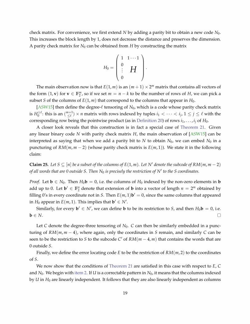
check matrix. For convenience, we first extend N by adding a parity bit to obtain a new code N0.This increases the block length by 1, does not decrease the distance and preserves the dimension.A parity check matrix for N0 can be obtained from H by constructing the matrix

H0 =

1 1 · · · 10

H...0

.

The main observation now is that E(1, m) is an (m + 1)× 2m matrix that contains all vectors ofthe form (1, v) for v ∈ Fm

2 , so if we set m = n− k to be the number of rows of H, we can pick asubset S of the columns of E(1, m) that correspond to the columns that appear in H0.

[ASW15] then define the degree-` tensoring of N0, which is a code whose parity check matrixis H⊗`0 : this is an (m+1

≤` )× n matrix with rows indexed by tuples i1 < · · · < ij, 1 ≤ j ≤ ` with thecorresponding row being the pointwise product (as in Definition 20) of rows i1, . . . , ij of H0.

A closer look reveals that this construction is in fact a special case of Theorem 21. Givenany linear binary code N with parity check matrix H, the main observation of [ASW15] can beinterpreted as saying that when we add a parity bit to N to obtain N0, we can embed N0 in apuncturing of RM(m, m− 2) (whose parity check matrix is E(m, 1)). We state it in the followingclaim:

Claim 25. Let S ⊆ [n] be a subset of the columns of E(1, m). Let N′ denote the subcode of RM(m, m− 2)of all words that are 0 outside S. Then N0 is precisely the restriction of N′ to the S coordinates.

Proof. Let b ∈ N0. Then H0b = 0, i.e. the columns of H0 indexed by the non-zero elements in badd up to 0. Let b′ ∈ Fn

2 denote that extension of b into a vector of length n = 2m obtained byfilling 0’s in every coordinate not in S. Then E(m, 1)b′ = 0, since the same columns that appearedin H0 appear in E(m, 1). This implies that b′ ∈ N′.

Similarly, for every b′ ∈ N′, we can define b to be its restriction to S, and then H0b = 0, i.e.b ∈ N.

Let C denote the degree-three tensoring of N0. C can then be similarly embedded in a punc-turing of RM(m, m − 4), where again, only the coordinates in S remain, and similarly C can beseen to be the restriction to S to the subcode C′ of RM(m− 4, m) that contains the words that are0 outside S.

Finally, we define the error locating code E to be the restriction of RM(m, 2) to the coordinatesof S.

We now show that the conditions of Theorem 21 are satisfied in this case with respect to E, Cand N0. We begin with item 2. If U is a correctable pattern in N0, it means that the columns indexedby U in H0 are linearly independent. It follows that they are also linearly independent as columns

19

in E(m, 1). Hence, using the same arguments as before we can find, for any coordinate v 6∈ U,a degree 2 polynomial g ∈ RM(2, m) such that g(v) = 1 and g restricted to U is 0. Restrictingthe evaluations of g to the subset of coordinates S, we get a codeword a ∈ E with the requiredproperty.

As for item 1: We first argue that RM(m, 2) ∗C′ ⊆ N′, since the degrees match and the propertyof vanishing outside S is preserved under multiplication. Projecting back to the coordinates in S,we get that E ∗ C ⊆ N0.

Acknowledgement

We would like thank Avi Wigderson, Emmanuel Abbe, Ilya Dumer, Venkatesan Guruswami andanonymous reviewers for helpful discussions and for commenting on an earlier version of thepaper.

References

[ALM+98] Sanjeev Arora, Carsten Lund, Rajeev Motwani, Madhu Sudan, and Mario Szegedy.Proof Verification and the Hardness of Approximation Problems. J. ACM, 45(3):501–555, 1998.

[Arı08] Erdal Arıkan. A Performance Comparison of Polar Codes and Reed-Muller Codes.IEEE Communications Letters, 12(6):447–449, 2008.

[AS92] Noga Alon and Joel H. Spencer. The Probabilistic Method. John Wiley, 1992.

[ASW15] Emmanuel Abbe, Amir Shpilka, and Avi Wigderson. Reed-Muller Codes for RandomErasures and Errors. In Proceedings of the 47th Annual ACM Symposium on Theory ofComputing (STOC 2015), pages 297–306, 2015. Pre-print available at arXiv:1411.4590.

[BF90] Donald Beaver and Joan Feigenbaum. Hiding instances in multioracle queries. InProceedings of the 7th Symposium on Theoretical Aspects of Computer Science (STACS 1990),pages 37–48, 1990.

[BFL91] Laszlo Babai, Lance Fortnow, and Carsten Lund. Non-Deterministic Exponential Timehas Two-Prover Interactive Protocols. Computational Complexity, 1:3–40, 1991. Prelim-inary version in the 31st Annual IEEE Symposium on Foundations of Computer Science(FOCS 1990).

[BL15] Abhishek Bhowmick and Shachar Lovett. The List Decoding Radius of Reed-MullerCodes over Small Fields. In Proceedings of the 47th Annual ACM Symposium on Theory ofComputing (STOC 2015), pages 277–285, 2015. Pre-print available at eccc:TR14-087.

20

[BV10] Andrej Bogdanov and Emanuele Viola. Pseudorandom Bits for Polynomials. SIAMJ. Comput., 39(6):2464–2486, 2010. Preliminary version in the 48th Annual IEEESymposium on Foundations of Computer Science (FOCS 2007). Pre-print available ateccc:TR14-081.

[CF07] Daniel J. Costello, Jr. and G. David Forney, Jr. Channel coding: The road to channelcapacity. Proceedings of the IEEE, 95(6):1150–1177, 2007.

[DK94] Iwan M. Duursma and Ralf Kotter. Error-locating pairs for cyclic codes. IEEE Transac-tions on Information Theory, 40(4):1108–1121, 1994.

[DS06] Ilya Dumer and Kirill Shabunov. Recursive error correction for general Reed-Mullercodes. Discrete Applied Mathematics, 154(2):253–269, 2006.

[Dum04] Ilya Dumer. Recursive decoding and its performance for low-rate Reed-Muller codes.IEEE Transactions on Information Theory, 50(5):811–823, 2004.

[Dum06] Ilya Dumer. Soft-decision decoding of Reed-Muller codes: a simplified algorithm.IEEE Transactions on Information Theory, 52(3):954–963, 2006.

[GKZ08] Parikshit Gopalan, Adam R. Klivans, and David Zuckerman. List-decoding Reed-Muller codes over small fields. In Proceedings of the 40th Annual ACM Symposium onTheory of Computing (STOC 2008), pages 265–274, 2008.

[GL89] Oded Goldreich and Leonid A. Levin. A Hard-Core Predicate for all One-Way Func-tions. In Proceedings of the 21st Annual ACM Symposium on Theory of Computing (STOC1989), pages 25–32, 1989.

[GRS14] Venkatesan Guruswami, Atri Rudra, and Madhu Sudan. Essential Coding The-ory. 2014. Available at http://www.cse.buffalo.edu/faculty/atri/courses/

coding-theory/book/.

[GS99] Venkatesan Guruswami and Madhu Sudan. Improved decoding of Reed-Solomonand algebraic-geometry codes. IEEE Transactions on Information Theory, 45(6):1757–1767, 1999.

[Ham50] R. W. Hamming. Error Detecting and Error Correcting Codes. Bell System TechnicalJournal, 26(2):147–160, 1950.

[HKL05] Tor Helleseth, Torleiv Kløve, and Vladimir I. Levenshtein. Error-correction capabilityof binary linear codes. IEEE Transactions on Information Theory, 51(4):1408–1423, 2005.

21

[KKM+16] Shrinivas Kudekar, Santhosh Kumar, Marco Mondelli, Henry D. Pfister, Eren Sasoglu,and Rudiger L. Urbanke. Reed-Muller codes achieve capacity on erasure channels. InProceedings of the 48th Annual ACM Symposium on Theory of Computing (STOC 2016),pages 658–669. ACM, 2016.

[Kri70] R. E. Krichevskiy. On the number of Reed-Muller code correctable errors. Dokl. Sov.Acad. Sci., 191:541–547, 1970.

[MHU14] Marco Mondelli, Seyed Hamed Hassani, and Rudiger L. Urbanke. From Polar to Reed-Muller Codes: A Technique to Improve the Finite-Length Performance. IEEE Transac-tions on Communications, 62(9):3084–3091, 2014.

[MS77] F. J. MacWilliams and N. J. A. Sloane. The theory of error correcting codes. Number v. 2in North-Holland mathematical library. North-Holland Publishing Company, 1977.

[Mul54] D. E. Muller. Application of Boolean algebra to switching circuit design and to er-ror detection. Electronic Computers, Transactions of the I.R.E. Professional Group on, EC-3(3):6–12, Sept 1954.

[MV97] Meena Mahajan and V. Vinay. Determinant: Combinatorics, Algorithms, and Com-plexity. Chicago J. Theor. Comput. Sci., 1997.

[Pel92] Ruud Pellikaan. On decoding by error location and dependent sets of error positions.Discrete Mathematics, 106-107:369–381, 1992.

[Ree54] Irving S. Reed. A class of multiple-error-correcting codes and the decoding scheme.Trans. of the IRE Professional Group on Information Theory (TIT), 4:38–49, 1954.

[Sha48] C. E. Shannon. A Mathematical Theory of Communication. The Bell System TechnicalJournal, 27:379–423, 623–656, 1948.

[Sha79] Adi Shamir. How to share a secret. Communications of the ACM, 22(11):612–613, 1979.

[Sha92] Adi Shamir. IP = PSPACE. J. ACM, 39(4):869–877, 1992.

[SP92] V. M. Sidel’nikov and A. S. Pershakov. Decoding of Reed-Muller Codes with a LargeNumber of Errors. Problems Inform. Transmission, 28(3):80–94, 1992.

[Sud97] Madhu Sudan. Decoding of Reed Solomon Codes beyond the Error-Correction Bound.J. Complexity, 13(1):180–193, 1997.

[Sud01] Madhu Sudan. Algorithmic Introduction to Coding Theory, 2001. Lecture Notes,available at http://people.csail.mit.edu/madhu/FT02/scribe/lect11.pdf.

22

[WB86] Lloyd R. Welch and Elwyn R. Berlekamp. Error correction for algebraic block codes,1986. US Patent 4,633,470.

23