efficiently inefficient markets for assets and asset...
TRANSCRIPT

Efficiently Inefficient Markets forAssets and Asset Management
Nicolae Garleanu and Lasse Heje Pedersen∗
This version: June 2017
Abstract
We consider a model where investors can invest directly or search for an asset man-
ager, information about assets is costly, and managers charge an endogenous fee. The
efficiency of asset prices is linked to the efficiency of the asset management market: if
investors can find managers more easily, more money is allocated to active management,
fees are lower, and asset prices are more efficient. Informed managers outperform after
fees, uninformed managers underperform, while the average manager’s performance de-
pends on the number of “noise allocators.” Small investors should remain uninformed,
but large and sophisticated investors benefit from searching for informed active man-
agers since their search cost is low relative to capital. Hence, managers with larger and
more sophisticated investors are expected to outperform.
Keywords: asset pricing, market efficiency, asset management, search, information
JEL Codes: D4, D53, D83, G02, G12, G14, G23, L10
∗Garleanu is at the Haas School of Business, University of California, Berkeley, CEPR, and NBER; e-mail: [email protected]. Pedersen is at AQR Capital Management, Copenhagen Business School, NewYork University, and CEPR; www.lhpedersen.com. We are grateful for helpful comments from Jules vanBinsbergen, Ronen Israel, Stephen Mellas, Jim Riccobono, Tano Santos, Andrei Shleifer, Peter NormanSørensen, and Morten Sørensen, as well as from seminar participants at Harvard University, New YorkUniversity, Chicago Booth, UC Berkeley, AQR Capital, CEMFI, IESE, Toulouse School of Economics,MIT Sloan, Imperial College, Cass Business School, Tinbergen Institute, Copenhagen Business School, andthe conferences at NBER Asset Pricing, Queen Mary University of London, the Cowles Foundation atYale University, the European Financial Management Association Conference, the 7th Erasmus LiquidityConference, the IF2015 Annual Conference in International Finance, the FRIC’15 Conference, and the KarlBorch Lecture. Pedersen gratefully acknowledges support from the European Research Council (ERC grantno. 312417) and the FRIC Center for Financial Frictions (grant no. DNRF102).

Asset managers play a central role in making financial markets efficient, as their size
allows them to spend significant resources on acquiring and processing information. The
asset management market is subject to its own frictions, however, since investors must search
for informed asset managers. Indeed, institutional investors literally fly around the world
to examine asset managers, assessing their investment process, trading infrastructure, risk
management, and so on. Similarly, individual investors search for asset managers, some via
local branches of financial institutions, others via the internet or otherwise.
How does this search for asset managers affect the efficiency of security markets? What
type of manager is expected to outperform? Which type of investors should use active
investing?
We seek to address these questions in a model with two levels of frictions: investors’ costs
of searching for informed asset managers and asset managers’ cost of collecting information
about assets. Despite this apparent complexity, the model is very tractable and delivers
several new predictions that link the levels of inefficiency in the security market and the
market for asset management: (1) If investors can find managers more easily, more money is
allocated to active management, fees are lower, and security prices are more efficient; (2) as
search costs diminish, asset prices become efficient in the limit, even if information-collection
costs remain large; (3) managers of assets with higher information costs earn larger fees and
are fewer, and such assets are less efficiently priced; (4) informed managers outperform after
fees while uninformed managers underperform after fees; (5) the net performance of the aver-
age manager depends on the number of “noise allocators” (who allocate to randomly chosen
managers) and, under certain conditions, is zero or negative; (6) searching for informed ac-
tive managers is attractive for large or sophisticated investors, while small or unsophisticated
investors should be uninformed; (7) managers with larger and more sophisticated investors
are expected to outperform.
As a way of background, the key benchmark is that security markets are perfectly efficient
(Fama (1970)), but this leads to two paradoxes: First, no one has an incentive to collect
information in an efficient market, so how does the market become efficient (Grossman and
1
Stiglitz (1980))? Second, if asset markets are efficient, then positive fees to active managers
implies inefficient markets for asset management (Pedersen (2015)).
Grossman and Stiglitz (1980) show that the first paradox can be addressed by considering
informed investing in a model with noisy supply, but, when an agent has collected information
about securities, she can invest on this information on behalf of others, so professional asset
managers arise naturally (Admati and Pfleiderer (1988), Ross (2005), Garcıa and Vanden
(2009)). Therefore, we introduce professional asset managers into the Grossman-Stiglitz
model.
One benchmark for the efficiency of asset management is provided by Berk and Green
(2004), who consider the implications of fully efficient asset-management markets (in the
context of exogenous and inefficient asset prices). In contrast, we consider an imperfect
market for asset management due to search frictions, consistent with the empirical evidence
of Sirri and Tufano (1998), Jain and Wu (2000), Hortacsu and Syverson (2004), and Choi
et al. (2010). We focus on investors’ incentive to search for informed managers and managers’
incentives to acquire information about assets with endogenous prices, abstracting from how
agency problems and imperfect contracting can distort asset prices (Shleifer and Vishny
(1997), Stein (2005), Cuoco and Kaniel (2011), Buffa et al. (2014)).
We employ the term efficiently inefficient to refer to the equilibrium level of inefficiency
given the two layers of frictions in the spirit of the Grossman-Stiglitz notion of “an equilibrium
degree of disequilibrium.” Paraphrasing Grossman-Stiglitz, prices in efficiently inefficient
markets reflect information, but only partially, so that some managers have an incentive to
expend resources to obtain information, but only part of the managers, so investors have an
incentive to expend resources to find informed managers.
Our equilibrium works as follows. Among the group of asset managers, an endogenous
number decide to acquire information about a security. Investors must decide whether to
expend search costs to find one of the informed asset managers. In an interior equilibrium,
investors are indifferent between searching for an informed asset manager vs. uninformed
investing (and both of these options dominate the investor collecting information herself). 1
1Investors do not collect information on their own, since the costs of doing so are higher than the benefits
2

When an investor meets an asset manager, they negotiate a fee, and asset prices are set in a
competitive noisy rational expectations market. The economy also features a group of “noise
traders” (or “liquidity traders”) who take random security positions as in Grossman-Stiglitz.
Likewise, we introduce a group of “noise allocators” who allocate capital to a random group
of asset managers, e.g., because they place trust in these managers as modeled by Gennaioli
et al. (2015).
We solve for the equilibrium number of investors who invest through managers, the
equilibrium number of informed asset managers, the equilibrium management fee, and the
equilibrium asset prices. The model features both search and information frictions, but the
solution is surprisingly simple and yields a number of clear new results.
First, we show that informed managers outperform before and after fees, while unin-
formed managers naturally underperform after fees. Investors who search for asset managers
must be compensated for their search and due diligence costs, and this compensation comes
in the form of expected outperformance after fees. Investors are indifferent between active
and uninformed investing in an interior equilibrium, so a larger search cost must be associ-
ated with a larger outperformance by active investors. Noise allocators invest partly with
uninformed managers and therefore may experience underperformance after fees. The asset-
weighted average manager (equivalently, their average investor) outperforms after fees if the
number of noise allocators is small, and underperforms if many noise allocators exist. When
the average manager outperforms, searching investors would have an incentive to “free ride”
by choosing a random manager if this were free, but all manager allocations require a search
cost in our baseline model. In a model extension with free search for a random manager, the
equilibrium outperformance of the average manager is zero or negative.
The model consequently helps explain a number of empirical regularities on the perfor-
mance of asset managers that are puzzling in light of the literature. Indeed, while the “old
consensus” in the literature was that the average mutual fund has no skill (Fama (1970),
to an individual due to the relatively high equilibrium efficiency of the asset markets. This high equilibriumefficiency arises from investors’ ability to essentially “share” information collection costs by investing throughan asset manager.
3

Carhart (1997)), a “new consensus” has emerged that the average hides significant cross-
sectional variation in manager skill among mutual funds, hedge funds, private equity, and
venture capital.2 For instance, Kosowski et al. (2006) conclude that “a sizable minority
of managers pick stocks well enough to more than cover their costs.” In our model, this
outperformance after fees is expected as compensation for investors’ search costs, but it is
puzzling in light of the prediction of Fama (1970) that all managers underperform after fees,
and the prediction of Berk and Green (2004) that all managers deliver zero outperformance
after fees. Further, the fact that top hedge funds and private equity managers deliver larger
outperformance than top mutual funds is consistent with our model under the assumption
that investors face larger search costs in these segments.
While the data support our novel prediction that some managers outperform others,
we can test the model at a deeper level by examining whether it can also explain who
outperforms. To do this, we extend the model by considering investors and asset managers
who differ in their size or sophistication. We show that large and sophisticated investors
benefit from searching for an informed manager, since their search cost is low relative to
their capital. In contrast, small unsophisticated investors are better served by uninformed
investing. As a result, active investors who are small must be noise allocators, while large
active investors could be rational searching investors (or noise allocators). Hence, we predict
that large investors perform better than small investors on average, because large investors
are more likely to find informed managers. This prediction is consistent with the findings
of Dyck and Pomorski (2016), who report that large institutional investors select managers
who outperform those of small investors.
We also predict that asset managers who have larger and more sophisticated investors
outperform those serving small unsophisticated investors. Consistent with this prediction,
managers of institutional investors outperform those of retail investors (Evans and Fahlen-
brach (2012), Dyck et al. (2013), Gerakos et al. (2016)).
2Evidence on mutual funds is provided by Grinblatt and Titman (1989), Wermers (2000), Kacperczyket al. (2008), Fama and French (2010), Berk and Binsbergen (2015), and Kacperczyk et al. (2014)), on hedgefunds by Kosowski et al. (2007), Fung et al. (2008), Jagannathan et al. (2010), and on private equity andventure capital by Kaplan and Schoar (2005).
4

The model also generates a number of implications of cross-sectional and time-series
variation in search costs. The important observation is that, if search costs are lower such
that investors more easily can identify informed managers, then more money is allocated
to active management, fees are lower, and security markets are more efficient. If investors’
search costs go to zero, then the asset market becomes efficient in the limit. Indeed, as
search costs diminish, fewer and fewer asset managers with more and more asset under
management collect smaller and smaller fees, and this evolution makes asset prices more
and more efficient even though information-collection costs remain constant (and potentially
large). It may appear surprising (and counter to the result of Grossman and Stiglitz (1980))
that markets can become close to efficient despite large information collection costs, but this
result is driven by the fact that the costs are shared by investors through an increasingly
consolidated group of asset managers.
These model-implied predictions are consistent with a number of empirical findings. For
instance, if search costs have diminished over time as information technology has improved,
markets should have become more efficient, consistent with the evidence of Wurgler (2000)
and Bai et al. (2013), and linked to the amount of assets managed by professional traders
(Rosch et al. (2015)).
In summary we complement the literature3 by introducing a new model of asset man-
agement and asset prices. The main innovation, search for managers, produces wide-ranging
results in a surprisingly tractable manner. Thinking through the logic of search markets
almost immediately yields new predictions on the performance of investors and managers,
while other predictions require a deeper model analysis, such as the magnitude of market
inefficiency (approximately 6%), fees, and the industrial organization of asset management.
The next section lays out the basic model, Section 2 provides the solution, and Section 3
derives the results. Section 4 extends the model to small and large investors and asset
3The related theoretical literature includes, beside the papers already cited, models of asset management(Pastor and Stambaugh (2012), Vayanos and Woolley (2013), Stambaugh (2014)), noisy rational expectationsmodels (Grossman (1976), Hellwig (1980), Diamond and Verrecchia (1981), Admati (1985)), other modelsof informed trading (Glosten and Milgrom (1985), Kyle (1985)), information acquisition (Van Nieuwerburghand Veldkamp (2010), Kacperczyk et al. (2014)), and search models in finance (Duffie et al. (2005), Lagos(2010)); we discuss the related empirical literature in Section 5.
5

managers. Section 5 discusses our empirical predictions and Section 6 concludes. Appendix A
contains further analysis and proofs and Appendix B describes the real-world issues related
to search and due diligence of asset managers.
1 Model of Assets and Asset Managers
1.1 Investors and Asset Managers
The economy features several types of competitive agents trading in a financial market, as
illustrated by Figure 1. Searching investors trade directly or through asset managers, asset
managers trade on behalf of groups of investors, noise allocators make random allocations
to asset managers, and noise traders make random trades in financial markets.
Specifically, the economy has A searching investors (or “allocators”), each of whom can
either (i) invest directly in asset markets after having acquired a signal s at cost k, (ii) invest
directly in asset markets without the signal, or (iii) invest through an asset manager. Due to
economies of scale, a natural equilibrium outcome is that investors do not acquire the signal,
but, rather, invest as uninformed or through a manager. We highlight below (see the end of
Section 2.3) some weak conditions under which all realistic equilibria take this form, and we
therefore rule out that investors acquire the signal. Consequently, we focus on the number
A of investors who make informed investments through a manager, inferring the number of
uninformed investors as the residual, A − A.
The economy has M risk-neutral asset-management firms.4 Of these asset managers,
only M elect to pay a cost k to acquire the signal s and thereby become informed asset
managers. The remaining M − M managers seek to collect asset management fees and
invest without information. The number of informed asset managers is determined as part
4The total number of asset managers M can be endogenized based on an entry cost ku for being anuninformed manager. Such an endogenous entry leaves the other equilibrium conditions unaffected when weinterpret the information cost k as the additional cost that informed managers must incur, i.e., their totalcost is ku + k. Asset management firms are risk-neutral as they face only idiosyncratic risk that can bediversified away by their owners.
6

Figure 1: Model Overview.
of the equilibrium.5
To invest with an informed asset manager, investors must search for, and vet, managers,
which is a costly activity. Specifically, the cost of finding an informed manager and confirming
that she has the signal (i.e., performing due diligence) is given by a general continuous
function c(M,A), which depends on both the number of informed asset managers M and
the number of their investors A.6 The search cost c captures the realistic feature that most
investors spend significant resources finding an asset manager they trust with their money,
as described in detail in Appendix B.
We assume that all investors have constant absolute risk aversion (CARA) utility over
end-of-period consumption with risk-aversion parameter γ (following Grossman and Stiglitz
(1980)). For convenience, we express the utility as certainty-equivalent wealth — hence,
with end-date wealth W , an investor’s utility is − 1γ
log(E(e−γW )). Each investor is endowed
with an initial wealth W .
5We note that we think of the sets of managers and investors as continua (e.g., M is the mass of informedmanagers), which keeps the exposition as simple as possible, but the model’s properties also obtain in a limitof a finite-investor model.
6We require continuity of c only on [0,∞)2 r {(0, 0)} as it is natural to assume that finding an informedmanager is infinitely costly if none exists, c(0, A) = ∞ for all A.
7

When an investor has found an asset manager and confirmed that the manager has the
technology to obtain the signal, they negotiate the asset management fee f . The fee is
set through Nash bargaining and, at this bargaining stage, all costs are sunk — both the
manager’s information acquisition cost and the investor’s search cost.7
We note that while the fee f is a total payment, which is the relevant quantity for
the agents’ utilities, it can be achieved through an unlimited number of combinations of
funds invested and percentage fees (as is typical in the literature). For instance, economic
outcomes are unchanged if investors double their dollar investment in the fund and pay half
the percentage fee, while the manager puts half of the portfolio in cash (or an index).
Lastly, the economy features a group of “noise traders” and one of “noise allocators.”
As in Grossman and Stiglitz (1980), noise traders buy an exogenous number of shares of
the security, q − q, as described below. Noise traders create uncertainty about the supply
of shares and are used in the literature to capture the fact that it can be difficult to infer
fundamentals from prices. Noise traders are also called “liquidity traders” in some papers
and their demand can be justified by a liquidity need, hedging demand, or behavioral reasons.
Following the tradition of noise traders, we introduce the concept of “noise allocators,”
of total mass N ≥ 0, who allocate their funds across randomly chosen asset managers.
Noise allocators play a similar role in the market for asset management to noise traders
in the market for assets — specifically, noise allocators can make it difficult for searching
investors to determine whether a manager is informed by looking at whether she has other
investors. Further, the existence of noise allocators changes the performance characteristics
across managers and investors, giving rise to novel model predictions, particularly when we
introduce agent heterogeneity in Section 4. Noise allocators pay the general fee f , which we
can view as an assumption for simplicity. However, this fee and behavior of noise allocators
are endogenized in Appendix A.4.
7Negotiation over terms is a common feature of the interaction between institutional investors and assetmanagers, but much less widespread for individual investors. For individual investors, our assumption canbe interpreted as the result of other forms of (imperfect) competition among managers, for instance as inGarcıa and Vanden (2009). The main feature needed is that the fee provides incentives to search.
8

1.2 Assets and Information
We adopt the asset-market structure of Grossman and Stiglitz (1980), aiming to focus on the
consequences of introducing asset managers into this framework. Specifically, there exists
a risk-free asset normalized to deliver a zero net return, and a risky asset with payoff v
distributed normally with mean v and standard deviation σv. Agents can obtain a signal s
of the payoff, where
s = v + ε. (1)
The noise ε has mean zero and standard deviation σε, is independent of v, and is normally
distributed.
The risky asset is available in a stochastic supply given by q, which is jointly normally
distributed with, and independent of, the other exogenous random variables. The mean
supply is q and the standard deviation of the supply is σq. We think of the noisy supply as
the number of shares outstanding q plus the supply q − q from the noise traders.
Given this asset market, uninformed investors buy a number of shares xu as a function of
the observed price p, to maximize their utility uu (certainty-equivalent wealth), taking into
account that the price p may reflect information about the value:
uu(W ) = −1
γlog
(
E
[
maxxu
E(e−γ(W+xu(v−p))|p
)])
= W + uu(0) ≡ W + uu. (2)
We see that, because of the CARA utility function, an investor’s wealth level simply shifts
his utility function and does not affect his optimal behavior. Therefore, we define the scalar
uu as the wealth-independent part of the utility function (a scalar that naturally depends
on the asset-market equilibrium, in particular the price efficiency).
Asset managers observe the signal and invest in the best interest of their investors. This
informed investing gives rise to the gross utility ui of an active investor (i.e., not taking into
account his search cost and the asset management fee — we study those, and specify their
9

impact on the ex-ante utility, later):
ui(W ) = −1
γlog
(
E
[
maxxi
E(e−γ(W+xi(v−p))|p, s
)])
= W + ui(0) ≡ W + ui. (3)
As above, we define the scalar ui as the wealth-independent part of the utility function. The
gross utility of an active investor differs from that of an uninformed via conditioning on the
signal s.
We note that all investors with an informed manager want the same portfolio xi since
investors are homogeneous. Hence, we simply assume that the manager offers the portfolio
xi for anyone investing W . When we introduce small and large investors in Section 4,
investors with smaller absolute risk aversions prefer larger multiples of the same xi, which
can naturally be achieved through a larger investment in the same fund.
1.3 Equilibrium Concept
We first consider the (partial) equilibrium in the asset market given the numbers of informed
and uninformed investors. We denote the mass of informed investors by I and note that it
is the sum of the number A of rational investors who decide to search for a manager and the
number of the noise allocators who happen to find an informed manager, where the latter is
the total number N of noise allocators times the fraction M/M of informed managers:
I = A + NM
M. (4)
Clearly, the remaining investors, A + N − I, invest as uninformed, either directly or via an
uninformed manager. An asset-market equilibrium is an asset price p such that the asset
market clears:
q = Ixi + (A + N − I)xu, (5)
10

where xi is the demand that maximizes the utility of informed investors (3) given p and the
signal s, and xu is the demand of uninformed investors (2). The market clearing condition
equates the noisy supply q with the total demand from all informed and uninformed investors.
Second, we define a general equilibrium for assets and asset management as a number
of informed asset managers M , a number of active investors A, an asset price p, and asset
management fees f such that (i) no manager would like to change her decision of whether
to acquire information, (ii) no investor would like to switch status from active (with an
associated utility of W +ui − c−f) to uninformed (conferring utility W +uu) or vice-versa,
(iii) the price is an asset-market equilibrium, and (iv) the asset management fees are the
outcome of Nash bargaining.
2 Solving the Model
2.1 Asset-Market Equilibrium
We first derive the asset-market equilibrium taking as given the number of informed investors
I. We later solve for the equilibrium number of searching investors and managers, which
yields I by (4). For a given I, the unique linear asset-market equilibrium is as in Grossman
and Stiglitz (1980), but for completeness we record the main results here. 8
In the linear equilibrium, an informed agent’s demand for the asset is a linear function
of prices and signals and the price is a linear function of the signal and the noisy supply:
p = θ0 + θs ((s − v) − θq(q − q)) , (6)
where the coefficients θ are given in Appendix A.5. The key property of the price is its
efficiency (or informativeness), which Grossman and Stiglitz (1980) define as var(v|s)var(v|p)
. For
8Our setup differs from the one of Grossman and Stiglitz (1980) by a change of variables, which leads tosome superficial differences in the results. Palvolgyi and Venter (2014) derive interesting non-linear equilibriain the Grossman and Stiglitz (1980) model.
11

convenience, we concentrate on the quantity
η ≡ log
(σv|p
σv|s
)
=1
2log
(var(v|p)
var(v|s)
)
, (7)
which represents the price inefficiency. This quantity records the amount of uncertainty
about the asset value for someone who only knows the price p, relative to the uncertainty
remaining when one knows the signal s. The price inefficiency is a positive number, η ≥ 0,
since the price is a noisy version of the signal, var(v|p) ≥ var(v|p, s) = var(v|s). Naturally,
a higher η corresponds to a more inefficient asset market and a zero inefficiency corresponds
to a price that fully reveals the signal.
The price inefficiency η is linked to investors’ value of information. Indeed, η gives
the relative utility of investing based on the manager’s information (ui) vs. investing as
uninformed (uu):
γ(ui − uu) = η. (8)
This is an important result because the relative utility ui − uu plays a central role in the
remainder of the paper, affecting investors’ incentive to search, asset management fees, and
managers’ incentive to acquire information.
The inefficiency η can be written as an explicit function of the number of informed
investors I:
η = −1
2log
(
1 −σ2
qσ2ε
I2/γ2 + σ2qσ
2ε
σ2v
σ2ε + σ2
v
)
∈ (0,∞). (9)
We see that η is decreasing in I, which is natural since, when there are more informed in-
vestors, asset prices become less inefficient (lower η), implying that informed and uninformed
investors receive more similar utilities (lower ui − uu).
We note that the price inefficiency does not depend directly on the the number of asset
managers M . What determines the asset price efficiency is the risk-bearing capacity of
agents investing based on the signal, and this risk-bearing capacity is ultimately determined
12

by the number of informed investors (not the number of managers they invest through).
The number of asset managers does affect asset price efficiency indirectly, however, since M
affects I as seen in (4), and, importantly, since the number of searching investors A and the
number of asset manages are determined jointly in equilibrium, as we shall see.
2.2 Asset Management Fee
The asset-management fee is set through Nash bargaining between an investor and a man-
ager. The bargaining outcome depends on each agent’s utility in the events of agreement vs.
no agreement (the latter is called the “outside option”). For the investor, the utility when
agreeing on a fee f is W − c − f + ui. If no agreement is reached, the investor’s outside
option is to invest as uninformed with his remaining wealth, yielding a utility of W − c + uu
as the cost c is already sunk.9 Hence, the investor’s gain from agreement is ui − uu − f .
Similarly, the asset manager’s gain from agreement is the fee f . This is true because the
manager’s information cost k is sunk and there is no marginal cost to taking on the investor.
The bargaining outcome maximizes the product of the utility gains from agreement:
maxf
(ui − uu − f) f. (10)
The solution is the equilibrium asset management fee f given by
f =η
2γ, [equilibrium asset management fee] (11)
using ui − uu = η/γ from equation (8). This equilibrium fee is simple and intuitive: The fee
would naturally have to be zero if asset markets were perfectly efficient, so that no benefit
of information existed (η = 0), and it increases in the size of the market inefficiency. Indeed,
active asset management fees can be viewed as evidence that investors believe that security
9The investor’s outside option is equal to the utility of searching again for another manager in an interiorequilibrium. Hence, we can think of the investor’s bargaining threat as walking away to invest on his own orto find another manager. Note also that we specify the bargaining objective in terms of certainty-equivalentwealth, which is natural and tractable.
13

markets are less than fully efficient.
We next derive the investors’ and managers’ decisions in an equally straightforward man-
ner. Indeed, an attractive feature of this model is that it is very simple to solve, yet provides
powerful results.
2.3 Investors’ Decision to Search for Asset Managers
An investor optimally decides to look for an informed manager as long as
ui − c − f ≥ uu. (12)
Recalling the equality η = γ(ui − uu), the investor’s optimality condition can be written as
η ≥ γ(c + f). This relation must hold with equality in an “interior” equilibrium (i.e., an
equilibrium in which strictly positive amounts of investors decide to invest as uninformed and
through asset managers — as opposed to all investors making the same decision). Inserting
the equilibrium asset management fee (11), we have already derived the investor’s indifference
condition: c = η2γ
.
Using similar straightforward arguments, we see that an investor would prefer using an
asset manager to acquiring the signal singlehandedly provided k ≥ c + f . Using the equilib-
rium asset management fee derived in equation (11), the condition that asset management
is preferred to buying the signal can be written as k ≥ 2c. In other words, finding an asset
manager should cost at most half as much as actually being one, which seems to be a condi-
tion that is clearly satisfied in the real world. We can also make use of (13) to express this
condition equivalently as A ≥ 2M , i.e., there must be at least two searching investors for
every manager, another realistic implication.
Finally, we note that we have assumed that searching investors only allocate to an active
manager when they have paid a search cost to ensure that the manager is informed. We
could also allow investors to pick a random manager without paying a search cost, even pick
a manager based on her assets under management (AUM). We consider such extensions in
14

Section 3.1.1 and Appendix A.2.
2.4 Entry of Informed Asset Managers
A prospective informed asset manager must pay the cost k to acquire information. Becoming
an informed manager has the benefit that the manager can expect to have more investors.
Specifically, each manager receives a noisy number of investors, but, since managers are risk
neutral, they optimize the expected fee revenue net of information costs.
An uninformed manager expects N/M investors, that is, the number of noise allocators
divided by the total number of managers. An informed manager expects A/M + N/M
investors since she expects a fraction of the searching investors in addition to the noise
allocators. Therefore, she chooses to become informed provided that the expected extra fee
revenue covers the cost of information:
fA
M≥ k. (13)
This manager condition must hold with equality for an interior equilibrium, and we can
easily insert the equilibrium fee (11) to get M = ηA2γk
.
2.5 General Equilibrium for Assets and Asset Management
We focus on interior equilibria, but we provide a complete equilibrium characterization in
Appendix A.1. We have arrived at the following two indifference conditions:
η(I)
2γ= c (M,A) [investors’ indifference condition] (14)
η(I)
2γ=
M
Ak, [asset managers’ indifference condition] (15)
where η is a function of I = A + N MM
given explicitly by (9). Hence, solving the general
equilibrium comes down to solving these two explicit equations in two unknowns (A,M).
Recall that a general equilibrium for assets and asset management is a four-tuple (p, f, A,M ),
15

but we have eliminated p by deriving the market efficiency η in a partial asset market
equilibrium and we have eliminated f by expressing it in terms of η. We can solve equations
(14)–(15) explicitly when the search-cost function c is specified appropriately as we show in
the following example, but the remainder of the paper provides results for general search-cost
functions.
Example: Closed-Form Solution. A cost specification motivated by the search literature
is
c (M,A) = c
(A
M
)α
for M > 0 and c(M,A) = ∞ for M = 0, (16)
where the constants α > 0 and c > 0 control the nature and magnitude of search frictions.
The idea is that informed asset managers are easier to find if a larger fraction of all asset
managers are informed, while performing due diligence (which requires the asset manager’s
time and cooperation) is more difficult in a tighter market with a larger number of searching
investors. With this search cost function, equations (14)–(15) can be combined to yield
η = 2γ (ckα)1
1+α , (17)
which shows how search costs and information costs determine market inefficiency η. We
then derive the equilibrium number of informed investors I from (9):
I = γσqσε
√σ2
v
σ2ε + σ2
v
1
1 − e−2η− 1 = γσqσε
√σ2
v
σ2ε + σ2
v
1
1 − e−4γ(ckα)1
1+α
− 1 . (18)
The number of informed managers can be linearly related to the number of searching investors
based on (15) and (17):
M =η
2γkA =
( c
k
) 11+α
A, (19)
16

so the number of managers per investor M/A depends on the magnitude of the search cost
c relative to the information cost k. Combining (19) with the identity I = A + M NM
yields
the solution for A
A = I
(
1 +N
M
( c
k
) 11+α
)−1
, (20)
concentrating on parameters for which A < A.
When η is small — a reasonable value is η = 6%, as we show in Section 3.3 — we can
approximate the number of informed investors more simply as
I ∼=γ
(2η)1/2
σqσεσv
(σ2ε + σ2
v)1/2
=γ1/2
2(ckα)1
2(1+α)
σqσεσv
(σ2ε + σ2
v)1/2
, (21)
illustrating more directly how search costs c and information costs k lower the number of
informed investors, while risk aversion γ and noise trading σq raise I.
Figure 2 provides a graphical illustration of the determination of equilibrium as the
intersection of the managers’ and investors’ indifference curves. The figure is plotted based
on the parametric example above,10 but it also illustrates the derivation of equilibrium for a
general search function c(M,A).
Specifically, Figure 2 shows various possible combinations of the numbers of active in-
vestors, A, and informed asset managers, M . The solid blue line indicates investors’ indif-
ference condition (14). When (A,M) is to the North-West of the solid blue line, investors
prefer to search for asset managers because managers are easy to find and attractive to find
due to the limited efficiency of the asset market. In contrast, when (A,M) is South-East
of the blue line, investors prefer to be uninformed as the costs of finding a manager is not
10We use the following parameters. Starting with the investors, the total number of optimizing investors isA = 108, the number of noise allocators is N = 108, the absolute risk aversion is γ = 3×10⁻⁵, correspondingto a relative risk aversion γR = 3 and an average invested wealth of W = 105. The total number of managersis M = 4, 000. Turning to asset markets, the number of shares outstanding is normalized to q = 1, theexpected final value of the asset equals total wealth v = (A + N)W = 2 × 10¹³, the asset volatility is 20%meaning that σv = 0.2v, the signal about the asset has a 30% noise, σε = 0.3v, and the noise in the supplyis 20% of shares outstanding, σq = 0.2. Lastly, the frictions are given by the cost of being an informed assetmanager k = 2 × 10⁷ and the search cost parameters α = 0.8 and c = 0.3.
17

outweighed by the benefits. The indifference condition is naturally increasing as investors
are more willing to be active when there are more asset managers.
Similarly, the dashed red line shows the managers’ indifference condition (15). When
(A,M) is above the red line, managers prefer not to incur the information cost k since too
many managers are seeking to service the investors. Below the red line, managers want to
become informed. Interestingly, the manager indifference condition is hump shaped for the
following reason: When the number of active investors increases from zero, the number of
informed managers also increases from zero, since the managers are encouraged to earn the
fees paid by searching investors. However, the total fee revenue is the product of the number
of active investors A and the fee f . The equilibrium fee f decreases with number of active
investors because active investment increases the asset-market efficiency, thus reducing the
value of the asset management service. Hence, when so many investors have become active
that this fee-reduction dominates, additional active investment decreases the number of
informed managers.
The economy in Figure 2 has two equilibria. In one equilibrium (A,M) = (0, 0), meaning
no investor searches for asset managers as there is no one to be found, and no asset manager
sets up operation because there are no investors. We naturally focus on the more interesting
equilibrium with A > 0 and M > 0.
Figure 2 also helps illustrate the set of equilibria more generally. First, if the search and
information frictions c and k are strong enough, then the blue line is initially steeper than
the red line and the two lines only cross at (A,M) = (0, 0), meaning that this equilibrium is
unique due to the severe frictions. Second, if frictions c and k are mild enough, then the blue
line ends up below the red line at the right-hand side of the graph with A = A. In this case,
all investors being active is an equilibrium. Lastly, when frictions are intermediate — as in
Figure 2 — the largest equilibrium is an interior equilibrium, i.e., A < A and M < M . We
focus on such interior equilibria since they are the most realistic and interesting ones. We
note that, while Figure 2 has only a single interior equilibrium, more interior equilibria may
exist for other specifications of the search cost function (e.g., because the investor indifference
18

0 0.5 1 1.5 2 2.5 3 3.5
x 107
0
200
400
600
800
1000
1200
1400
1600
Number of searching investors, A
Num
ber
of in
form
ed a
sset
man
ager
s, M
investorssearch
investorspassive
managersexit
managersenter
Investor indifference conditionManager indifference condition
Figure 2: Equilibrium for assets and asset management. Illustration of the equilib-rium determination of the number of searching investors A and the number of informed assetmanagers M . Each investor decides whether to search for an asset manager or invest un-informed depending on the actions (A,M) of everyone else, and, similarly, managers decidewhether or not to acquire information. The right-most crossing of the indifference conditionsis an interior equilibrium.
condition starts above the origin, or because it can in principle “wiggle” enough to create
additional crossings of the two lines).
3 Equilibrium Properties
3.1 Performance of Asset Managers and Investors
We start by considering some basic properties of performance in efficiently inefficient markets.
We use the term outperformance to mean that an informed investor’s performance yields a
higher expected utility than that of an uninformed, and vice versa for underperformance.
We note that an investor’s expected utility is directly linked to his (squared) Sharpe ratio,
19
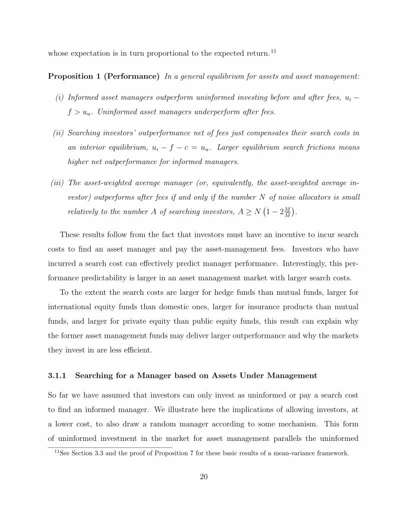
whose expectation is in turn proportional to the expected return.11
Proposition 1 (Performance) In a general equilibrium for assets and asset management:
(i) Informed asset managers outperform uninformed investing before and after fees, ui −
f > uu. Uninformed asset managers underperform after fees.
(ii) Searching investors’ outperformance net of fees just compensates their search costs in
an interior equilibrium, ui − f − c = uu. Larger equilibrium search frictions means
higher net outperformance for informed managers.
(iii) The asset-weighted average manager (or, equivalently, the asset-weighted average in-
vestor) outperforms after fees if and only if the number N of noise allocators is small
relatively to the number A of searching investors, A ≥ N(1 − 2M
M
).
These results follow from the fact that investors must have an incentive to incur search
costs to find an asset manager and pay the asset-management fees. Investors who have
incurred a search cost can effectively predict manager performance. Interestingly, this per-
formance predictability is larger in an asset management market with larger search costs.
To the extent the search costs are larger for hedge funds than mutual funds, larger for
international equity funds than domestic ones, larger for insurance products than mutual
funds, and larger for private equity than public equity funds, this result can explain why
the former asset management funds may deliver larger outperformance and why the markets
they invest in are less efficient.
3.1.1 Searching for a Manager based on Assets Under Management
So far we have assumed that investors can only invest as uninformed or pay a search cost
to find an informed manager. We illustrate here the implications of allowing investors, at
a lower cost, to also draw a random manager according to some mechanism. This form
of uninformed investment in the market for asset management parallels the uninformed
11See Section 3.3 and the proof of Proposition 7 for these basic results of a mean-variance framework.
20

investment in the security market in Grossman and Stiglitz (1980), that is, investment based
on freely available information. To make this alternative as attractive as possible, we take
this search cost to be zero and, furthermore, make it more likely to draw a larger manager.
To be precise, we assume that the investor obtains the industry-wide after-fee return. We
analyze this extended model in Appendix A.2. As an alternative, we consider below an
example in which investor are allowed to condition on all managers’ AUM.
For some parameters, the equilibrium in the baseline model is the same as the equilib-
rium in the extended model. Indeed, if the asset-weighted net return is worse than from
uninformed investing, which can be determined based on the condition in Proposition 1(iii),
then the equilibrium does not change as this search for a random manager is not attractive.
If not, then the equilibrium in the extended model changes: some investors will switch
from being uninformed or active to searching for a random manager, until the point at which
the asset-weighted manager’s net performance matches that of uninformed investing.
Proposition 1b. In the equilibrium of the extended model, the asset-weighted manager’s
outperformance after fees is zero (interior equilibrium) or negative, pIui+(1−pI)uu−f ≤ ui,
where pI is the fraction of assets managed by informed managers.
Hence, it may be no coincidence that the average manager in the data delivers a simi-
lar performance to index funds. Said differently, in an interior equilibrium of our extended
model, the assumption of Berk and Green (2004) that asset managers deliver a zero outper-
formance after fees holds at the level of the overall asset management industry, but not at
the level of each individual manager.
To understand the intuition for this result, start by recalling that an asset manager’s AUM
is noisy. Hence, while informed managers have higher AUM on average, any one informed
manager could have lower AUM than any one uninformed manager by chance. Therefore,
picking managers based on their AUM results in a mixture of informed and uninformed
ones. Further, while informed managers are expected to outperform net of fees, uninformed
21

managers underperform after fees (because they charge a fee even though they don’t add
value). Therefore, a mixture of these can be (and, indeed, will be, in an interior equilibrium)
just as good as direct uninformed investing and just as good as paying a search cost to find
a manager who is surely informed.
Example: distribution of manager size and performance. The underperformance of
the uninformed managers (−f) is as large in magnitude as the outperformance of informed
managers (ui − f − uu = f). Therefore, picking a random manager is a good investment
if the chance of getting an informed manager is at least 50%. In the numerical example of
Section 2.5, there are more uninformed than informed managers in equilibrium, so picking
a random manager would not be a good investment even if it were free. However, the
informed managers have more investors on average, so investing with the “market portfolio”
of managers would be better. Nevertheless, such an AUM-weighted manager investment is
also dominated by investing directly as uninformed in the example.
We can further refine the example to explicitly consider the size distribution across asset
managers. For instance, suppose that each manager receives a number of noise allocators
that is exponentially distributed with mean N/M (i.e., exponential parameter M/N). This
distribution can arise if noise allocators invest based on news stories, and news stories about
each manager arrive at Poisson jumps such that each manager receives media attention for an
exponentially-distributed time period. Each informed manager also receives A/M searching
investors for sure (i.e., without randomness, for simplicity).
In this case, managers with fewer than A/M investors must be uninformed. Among
managers with any number of investors greater than A/M , a constant proportion — 47%,
given the parameters of our numerical example — are informed, and the remainder — 53%
— are uninformed.12 Hence, if we further extended the model to allow investors to pick a
manager at any specific size (at some cost), then investors would not want to do so given
that only 47% of managers are informed. Instead, investors would still prefer to either pay
12Specifically, this proportion equals MeMN
AM /(Me
MN
AM + M − M).
22

a search cost to ensure finding an informed manager for sure or invest as uninformed.
3.1.2 On the Impossibility of Efficient Asset Management: A Paradox
The Grossman-Stiglitz paradox shows that security markets cannot be fully efficient since,
if they were, no one would have an incentive to collect information. A similar paradox exists
for asset management markets: public signals about asset managers such as their AUM
cannot fully reveal which managers are informed since, if they did, no investor would have
an incentive to search and do due diligence. This insight can be seen rigorously in the version
of our model in which investors can invest based on AUM for free. If the number of noise
allocators goes to zero, then AUM becomes very informative, leading fewer investors to pay
for search, and, eventually, the only equilibrium is one in which no investor searches and
no manager is informed. This equilibrium is fragile, however, as the market is so inefficient
that investors have strong incentives to find an informed manager (should any exist) — but,
as soon as someone succeeds in finding an informed manager, other investors can free ride.
Thus, noise allocators are needed to resolve this paradox just as noise traders are needed for
the Grossman-Stiglitz paradox.
3.1.3 Meaning of Efficiently Inefficient
We say that the asset price is fully efficient if η = 0, meaning that the price fully reflects
the signal. In equilibrium, asset prices always involve some degree of inefficiency (η > 0),
but efficiency can arise as a limit, as we shall see in the next section.
There can be several measures of the inefficiency of asset management markets. One mea-
sure of this inefficiency is the aggregate cost of locating asset managers plus their aggregate
information cost, cA + kM . As we shall see next, this aggregate asset management ineffi-
ciency can be reduced towards zero if the search cost is reduced. Another measure of asset
management efficiency could be the extent to which AUM reflects a manager’s information
as discussed in the paradox above.
We employ the term efficiently inefficient to refer to the equilibrium level of inefficiency
23

given the frictions (as discussed in the introduction). This definition applies both to markets
for securities and asset managers.
3.2 Comparative Statics
We next consider how the economic outcomes depend on the exogenous parameters. To
analyze such comparative statics in a model that could have multiple equilibria, we focus on
the equilibrium with the largest value of I simply because we need to pick a given equilibrium.
We start with the implications of changing the search cost:
Proposition 2 (Search for asset management)
(i) Consider two search cost functions, c1 and c2, with c1 > c2 and the corresponding
largest-I equilibria. In the equilibrium with the lower search costs c2, the numbers of
active investors A and of informed investors I are larger, the number of managers M
may be higher or lower, the asset price is more efficient, the asset management fee f
is lower, and the total fee revenue f(A + N) may be either higher or lower.
(ii) If {cj}j=1,2,3,... is a decreasing series of cost functions that converges to zero at every
point, then A = A when the cost is sufficiently low, that is, all rational agents search
for managers. If the number of investors {Aj} increases towards infinity as j goes to
infinity, then η goes to zero (full price efficiency in the limit), the asset management fee
f goes to zero, the number of asset managers M goes to zero, the number of investors
per manager goes to infinity, and the total fee revenue of all asset managers f(A + N)
goes to zero.
This proposition provides several intuitive results, which we illustrate in Figure 3. As seen
in the figure, a lower search costs means that the investor indifference curve moves down,
leading to a larger number of active investors in equilibrium. This result is natural, since
investors have stronger incentives to enter when their cost of doing so is lower.
The number of asset managers can increase or decrease (as in the figure), depending on
the location of the hump in the manager indifference curve. This ambiguous change in M
24

0 0.5 1 1.5 2 2.5 3 3.5
x 107
0
200
400
600
800
1000
1200
1400
1600
Number of searching investors, A
Num
ber
of in
form
ed a
sset
man
ager
s, M
Investor indifference conditionInvestor condition, lower search costManager indifference condition
Figure 3: Equilibrium effect of lower investor search costs. The figure illustrates thatlower costs of finding asset managers implies more active investors in equilibrium and, hence,increased asset-market efficiency.
is due to two countervailing effects. On the one hand, a larger number of active investors
increases the total management revenue that can be earned given the fee. On the other hand,
more active investors means more efficient asset markets, leading to lower asset management
fees. When the search cost is low enough, the latter effect dominates and the number of
managers starts falling as seen in part (ii) of Proposition 2.
As search costs continue to fall, the asset-management industry becomes increasingly
concentrated, with fewer and fewer asset managers managing the money of more and more
investors. This leads to an increasingly efficient asset market and market for asset manage-
ment.
Perhaps surprisingly, the security market can become almost efficient despite a high
Grossman-Stiglitz cost k. This finding is driven by the fact that, as search costs diminish,
investors essentially share the information cost more and more efficiently. Indeed, the aggre-
gate information cost incurred is kM , which decreases towards zero as the asset management
industry consolidates.
25

We next consider the effect of changing the cost of acquiring information, which depends
on some realistic properties of the search function.13
Proposition 3 (Information cost) Suppose that c satisfies ∂c∂M
≤ 0 and ∂c∂A
≥ 0. As the
cost of information k decreases, the largest equilibrium changes as follows: The number of
informed investors I increases, the number of asset managers M increases, the asset-price
efficiency increases, and the asset-management fee f goes down. The number of active
investors A may increase or decrease.
The results of this proposition are illustrated in Figure 4. As seen in the figure, a lower
information cost for asset managers moves their indifference curve out. This leads to a
higher number of asset managers and informed investors in equilibrium, which increases the
asset-price efficiency. Finally, we consider the effect of risk.
Proposition 4 (Risk) Suppose that ∂c∂M
≤ 0 and ∂c∂A
≥ 0. An increase in the fundamental
volatility σv or in the noise-trading volatility σq leads to a larger number of active investors
A, informed investors I, and informed asset managers M . The effect on the efficiency of
asset prices and the asset-management fee f , as well as the total fee revenues f(A + N), is
ambiguous. The same results obtain with a proportional increase in (σv, σε) or in all risks
(σv, σε, σq).
3.3 Economic Magnitude of Market Inefficiency
The debate in financial economics is often centered around whether the market is inefficient or
not. However, the Grossman-Stiglitz insight implies that we should really ask how inefficient.
Our model can help provide an answer. As we show below, the answer is neither “yes” nor
“no,” but “6%.”
13Proposition 3 relies on a regularity condition on the search cost function c. On one hand, finding aninformed manager is easier if a larger fraction of all managers are informed: ∂c
∂M ≤ 0. On the other, it is morechallenging if more other investors are competing for the asset manager’s time and attention: ∂c
∂A ≥ 0. Thismay be, for instance, why many managers have a minimum investment size. That said, there are potentialchannels, such as word-of-mouth communication, through which a larger number of searching investors mayalleviate search costs. Our condition is satisfied for the search cost function considered in our example inequation (16).
26

0 0.5 1 1.5 2 2.5 3 3.5
x 107
0
200
400
600
800
1000
1200
1400
1600
Number of searching investors, A
Num
ber
of in
form
ed a
sset
man
ager
s, M
Investor indifference conditionManager indifference conditionManager condition, lower information cost
Figure 4: Equilibrium effect of lower information acquisition costs. The figureillustrates that lower costs of getting information about assets implies more active investorsand more asset managers in equilibrium and, hence, increased asset-market efficiency.
To illustrate the economic magnitudes of some of the interesting properties of the model
in a simple way, it is helpful to write our predictions is relative terms. Specifically, as seen
in Section 4, investors’ preferences can be written in terms of the relative risk aversion γR
and wealth W such that γ = γR/W . Further, the asset management fee can be viewed as
a fixed proportion of the investment size and we define the proportional fee as f% = f/W .
To be specific, suppose that all investors have relative risk aversion of γR = 3 and that the
equilibrium percentage asset management fee is f% = 1%.
We can now link the market inefficiency η to the proportional asset management fee and
relative risk aversion,
η = 2fγ = 2f%γR = 2 ∙ 1% ∙ 3 = 6%. (22)
In other words, the standard deviation of the true asset value from the perspective of a
trader who knows the signal is 6% smaller than that of a trader who only observes the price.
27

Further, we see that the inefficiency is greater in markets with higher percentage fees (e.g.,
private equity vs. public) and during times of high risk aversion (e.g., crisis periods).
We can also characterize the inefficiency by the difference in squared gross Sharpe ratios
attainable by informed (SRi) vs. uninformed (SRu) investors using a log-linear approxima-
tion:14
E(SR2i ) − E(SR2
u)∼= 2η = 4f%γR = 4 ∙ 1% ∙ 3 = 0.12. (23)
Hence, if uninformed investing yields an expected squared Sharpe ratio of 0 .42 (similar to
that of the market portfolio), informed investing must yield an expected squared Sharpe
ratio around 0.532 (i.e., 0.532 − 0.42 = 0.12). We see that, at this realistic fee level, the
implied difference in Sharpe ratios between informed and uninformed managers is relatively
small and hard to detect empirically. While the model-predicted magnitude of inefficiency
appears reasonable, our model is of course quite stylized and needs to be supplemented with
empirical analysis.
4 Small vs. Large Investors and Asset Managers
So far, we have considered an economy in which all investors and managers are identical ex
ante, but, in the real world, investors differ in their wealth and financial sophistication and
managers differ in their education and investment approach. Should large asset owners such
as high-net-worth families, pension funds, or insurance companies invest differently than
small retail investors and what type of asset managers are more likely to be informed?
To address these issues, we extend the model to capture different types of investors and
managers. Each investor a ∈ [0, A] has an investor-specific search cost ca, where a smaller
14Since each type of investor n = i, u chooses a position of x = En(v)−pγVarn(v) , the investor’s conditional
Sharpe ratio is SRn = |En(v)−p|√Varn(v)
(where En and Varn are the mean and variance conditional on n’s infor-
mation). We have η = log(E[e−
12 (v−p)
E[v−p|p]var(v|p)
])− log
(E[e−
12 (v−p)
E[v−p|s,p]var(v|s)
]), which is approximated by
12
(E[(v − p)E[v−p|s,p]
var(v|s)
]− E
[(v − p)E[v−p|p]
var(v|p)
]), yielding (23) because the conditional variances are constant.
28

search cost corresponds to greater sophistication. Further, investors have different levels
of absolute risk aversion, γa. We can interpret these as arising from different wealth Wa
or different relative risk aversions γRa , corresponding to a constant absolute risk aversion
of γa = γRa /Wa.
15 The characteristics ca, γRa , and Wa are drawn randomly, independently
of each other and across agents. Also, noise allocators n ∈ [0, N ] have (cn, γRn ,Wn) drawn
independently from the same distribution.16
To capture different types of asset managers, we assume that each manager m ∈ [0, M ]
has a manager-specific cost km of becoming informed — one can think of this feature as skill
or education — and that they are ordered according to this cost. Hence, managers with
lower index m have lower costs, that is, the function k : [0, M ] → R is increasing.
We solve the model similarly to before, but we leave the details to Appendix A.3.
4.1 Who Should be Active?
We first study which types of investors should search for an active manager:
Proposition 5 (Which investors should be active?) An investor a should invest with
an active manager if he has a large wealth Wa, low relative risk aversion γRa , or low search
cost ca, all relative to the asset-market inefficiency η, that is, if
γRa ca
Wa
= γaca ≤1
2η, (24)
and otherwise should invest as uninformed.
This result is intuitive and consistent with the idea that the active investors should be
those who have a comparative advantage in asset allocation, either large investors who can
hire a serious manager-selection team or sophisticated investors with special insights on
15Wealth levels vary a lot more in the cross-section — easily by factors measured in thousands — thanrelative risk aversions, so that variation in γa is likely mostly driven by wealth differences in the real world.
16These independence assumptions only affect our performance results and we note that these resultswould only be strengthened under the realistic assumptions that high sophistication (low c) correlates withhigh wealth W , or if noise allocators are more likely to have low sophistication and wealth.
29
asset managers. Indeed, the cost of finding and vetting an informed asset manager is a
smaller fraction of the investment for large investors as is captured by equation (24). In
contrast, small retail investors are better served by low-cost uninformed investing. The next
proposition states the corresponding result for asset managers.
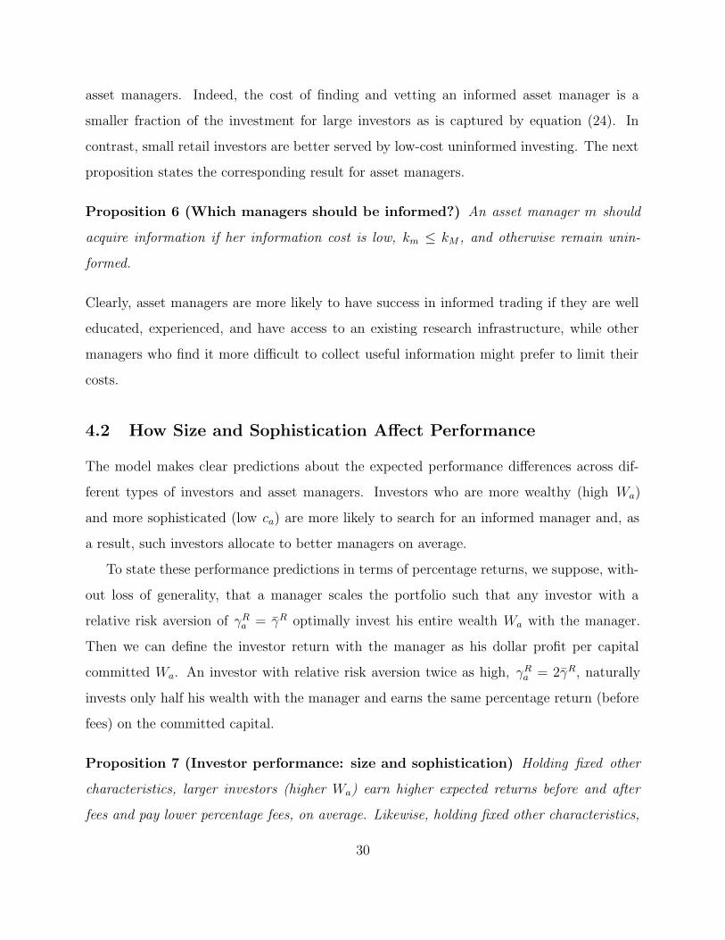
Proposition 6 (Which managers should be informed?) An asset manager m should
acquire information if her information cost is low, km ≤ kM , and otherwise remain unin-
formed.
Clearly, asset managers are more likely to have success in informed trading if they are well
educated, experienced, and have access to an existing research infrastructure, while other
managers who find it more difficult to collect useful information might prefer to limit their
costs.
4.2 How Size and Sophistication Affect Performance
The model makes clear predictions about the expected performance differences across dif-
ferent types of investors and asset managers. Investors who are more wealthy (high Wa)
and more sophisticated (low ca) are more likely to search for an informed manager and, as
a result, such investors allocate to better managers on average.
To state these performance predictions in terms of percentage returns, we suppose, with-
out loss of generality, that a manager scales the portfolio such that any investor with a
relative risk aversion of γRa = γR optimally invest his entire wealth Wa with the manager.
Then we can define the investor return with the manager as his dollar profit per capital
committed Wa. An investor with relative risk aversion twice as high, γRa = 2γR, naturally
invests only half his wealth with the manager and earns the same percentage return (before
fees) on the committed capital.
Proposition 7 (Investor performance: size and sophistication) Holding fixed other
characteristics, larger investors (higher Wa) earn higher expected returns before and after
fees and pay lower percentage fees, on average. Likewise, holding fixed other characteristics,
30

more sophisticated investors (lower ca) earn higher expected returns before and after fees and
pay lower percentage fees.
These results are intuitive and give rise to several testable predictions that we confront
with the existing evidence in Section 5. Since large and sophisticated investors can better
afford to spend resources on finding an informed manager, they are more likely to find one
and, as a result, they expect to earn higher returns.17 The higher returns are partly a
compensation for the search costs that these agents incur, but they can even outperform
after search costs when inequality (24) is strict.
Said differently, if a small investor with no special knowledge of asset managers (that is,
an investor for whom (24) is not satisfied) invests with an active manager, then he must be a
noise allocator. Since noise allocators pay fees even to uninformed managers, such investors
are expected to earn lower returns.
On the other hand, noise allocators are under-represented among large sophisticated
investors. We note that the model-implied effect is not linear in that, as investors become
very large (or sophisticated), they search for a manager almost surely, and therefore an even
larger size has a negligible effect on their expected performance. We next consider how
performance varies across asset managers.
Proposition 8 (Asset manager performance)
(i) Asset manager returns (before and after fees) and their average investor size covary
positively. Similarly, returns and average sophistication covary positively.
(ii) Asset-manager size and expected returns (before and after fees) covary positively. Sim-
ilarly, managers with a comparative advantage in collecting information (km ≤ kM)
earn higher expected returns before and after fees.
Part (i) shows that asset managers with larger and more sophisticated investors are
more likely to have investors who have performed due diligence and confirmed that they
17The fact that investors with large absolute risk tolerance choose informed investing through managers(by paying search costs and fees) parallels the result of Verrecchia (1982) that more risk-tolerant investorspurchase more precise (and expensive) signals.
31

are informed about security markets. These managers, being more likely to have passed a
screening, should deliver higher expected return on average (even though some of them can
still be uninformed as some large investors can also be noise allocators). Other measures
proxying for the type of a manager’s clientele, such as the proportion of large investors (i.e.,
with wealth above a given threshold), would work as well.
Part (ii) shows that managers who find it easier to collect information are more likely to
do it. Indeed, for the marginal manager, the cost of information equals the benefit, so anyone
with higher costs will not acquire information. Hence, an asset manager may be more likely
to be informed if she is well educated, experienced, and benefits from firm-wide investment
research as part of an investment firm with multiple funds. Hence, investors’ search process
might partly consist of examining whether an asset manager has such qualities, as discussed
further in Appendix B.
5 Empirical Implications
Our model has implications for investors, asset managers, and financial markets — three
layers that we represent schematically in Figure 5. We start by examining the predictions
and empirical evidence at the middle level, i.e., concerning managers.
5.1 Performance of Asset Managers
The central prediction of asset market efficiency is that all managers underperform by an
amount equal to their fees, and, indeed, the early empirical literature documented negative
average after-fee returns for US mutual funds (Fama (1970)). More recent evidence suggests
that the average alpha after fees is close to zero (Berk and Binsbergen (2015)). Further,
the research over the past decades shows that the evidence for the average asset manager
hides significant cross-sectional variation across managers. Indeed, the literature documents
a significant difference between the net-of-fee performance of the best and worst managers
of mutual funds (Kosowski et al. (2006), Kacperczyk et al. (2008), Fama and French (2010),
32

Sophisticatedinvestors
Goodsecurities
Badsecurities
Noiseallocators
Good assetmanagers
Bad assetmanagers
Figure 5: Testing the model at three levels. The figure illustrates stylistically thethree layers for which our model has new cross-sectional implications: investors, asset man-agers, and financial markets. Further, the model also makes predictions on the interactionbetween these layers, that is, the interaction between investors, securities, and the industrialorganization of asset management.
Keswani et al. (2016)), hedge funds (Kosowski et al. (2007), Fung et al. (2008), Jagannathan
et al. (2010)), private equity, and venture capital funds (Kaplan and Schoar (2005)). For
instance, Kosowski, Naik, and Teo (2007) report that “top hedge fund performance cannot
be explained by luck, and hedge fund performance persists at annual horizons... Our results
are robust and relevant to investors as they are neither confined to small funds, nor driven
by incubation bias, backfill bias, or serial correlation.”
The strong performance of the best managers presents a rejection of Fama’s hypothesis
that asset markets are fully efficient and all asset managers underperform by their fees.
Further, the net-of-fee performance spread between the best and worst managers is a rejection
of the hypothesis by Berk and Green (2004) that all managers deliver the same expected
net-of-fee return. The existence of the performance spread is, however, consistent with our
model’s predictions. In our model, top asset managers should be difficult to locate and their
outperformance must compensate investors for their search costs.
We note the following subtlety concerning the relation between our model and empirical
tests: Our model implies that investors should be able to find managers that outperform net
33
of fees only after incurring a search cost, but, then, should an empirical researcher be able
to identify such managers? On one hand, researchers should not be able to locate informed
managers based on public information that investors can easily process (as seen in the version
of our model where investors can search for free based on AUM, Section 3.1.1). On the other
hand, skilled researchers using large commercial databases and advanced statistical methods
would be able to locate informed managers, to the extent that this research mimics in part
investors’ costly search process. Of course, investors with access to more data (e.g., meetings
with managers that reveal the trading infrastructure) should be able to do even better.
Again, there is a close parallel between the market for assets and the market for asset
management: Just like finding good asset managers should be difficult, but not impossible,
finding good securities should also be difficult, but not impossible. In both cases, researchers
may identify good managers and good securities based on commercial data that are costly to
process. For instance, asset pricing anomalies are typically based on such commercial data.
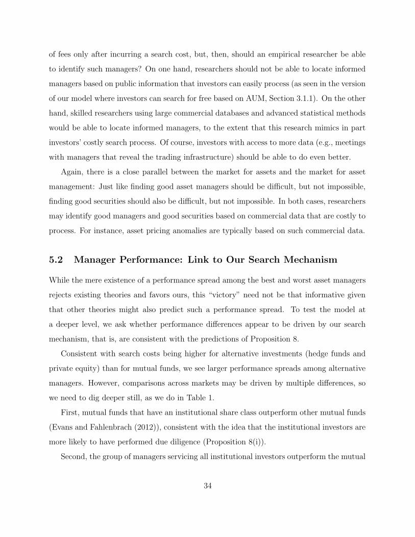
5.2 Manager Performance: Link to Our Search Mechanism
While the mere existence of a performance spread among the best and worst asset managers
rejects existing theories and favors ours, this “victory” need not be that informative given
that other theories might also predict such a performance spread. To test the model at
a deeper level, we ask whether performance differences appear to be driven by our search
mechanism, that is, are consistent with the predictions of Proposition 8.
Consistent with search costs being higher for alternative investments (hedge funds and
private equity) than for mutual funds, we see larger performance spreads among alternative
managers. However, comparisons across markets may be driven by multiple differences, so
we need to dig deeper still, as we do in Table 1.
First, mutual funds that have an institutional share class outperform other mutual funds
(Evans and Fahlenbrach (2012)), consistent with the idea that the institutional investors are
more likely to have performed due diligence (Proposition 8(i)).
Second, the group of managers servicing all institutional investors outperform the mutual
34
funds servicing retail investors (Gerakos et al. (2016)). Indeed, Gerakos et al. (2016) find
that the asset managers servicing institutions overall delivered outperformance after fees, in
contrast to the evidence on the average retail mutual fund discussed above.
Third, Guercio and Reuter (2014) find that mutual funds sold directly to searching in-
vestors outperform those that are placed via brokers who earn commissions/loads (to noise
allocators).
Fourth, consistent with Proposition 8(ii), Chevalier and Ellison (1999) find that “man-
agers who attended higher-SAT undergraduate institutions have systematically higher risk-
adjusted excess returns’ ’ and Chen et al. (2004) find that “Controlling for fund size [...] the
assets under management of the other funds in the family that the fund belongs to actually
increase the fund’s performance.”
Last, consistent with Proposition 1(ii), the outperformance of managers of searching
investors is larger in less efficient markets. Dyck et al. (2013) find that “active management
in emerging market equity outperforms passive strategies by more than 180 bps per year, and
that this outperformance generally remains significant when controlling for risk through a
variety of mechanisms. In EAFE equities (developed markets of Europe, Australasia, and the
Far East), active management also outperforms, but only by about 50 bps per year, consistent
with these markets being relatively more competitive and efficient.” Together, these findings
provide significant and diverse evidence for the model’s performance predictions.
From investors’ perspective, the relevant measure of manager performance is average
excess return (or alpha), but, when evaluating managers’ skill per se, Berk and Binsbergen
(2015) argue that the manager’s “value added” is a better measure. They find that the “cross-
sectional distribution of managerial skill is predominantly reflected in the cross-sectional
distribution of fund size,” a result consistent with the prediction of our Proposition 8(ii).
5.3 Investor Performance: Link to Our Search Mechanism
We now turn to the predictions for the top layer of Figure 5, namely investors. We have al-
ready discussed that institutional investors outperform even after fees (Gerakos et al. (2016)),
35
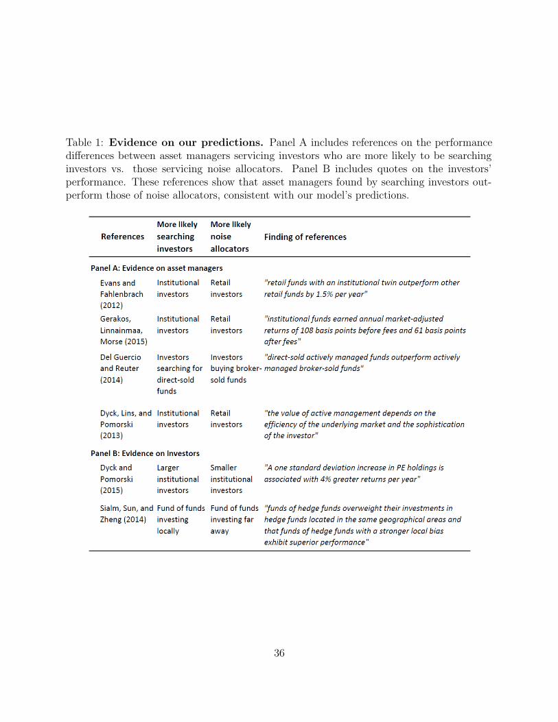
Table 1: Evidence on our predictions. Panel A includes references on the performancedifferences between asset managers servicing investors who are more likely to be searchinginvestors vs. those servicing noise allocators. Panel B includes quotes on the investors’performance. These references show that asset managers found by searching investors out-perform those of noise allocators, consistent with our model’s predictions.
36
hence performing better than the overall group of retail investors in their active mutual fund
allocations. This mirror image of the result for asset managers is consistent with Proposi-
tion 7.
Further, as seen in Panel B of Table 1, Dyck and Pomorski (2016) find that large in-
stitutions outperform small ones in their private equity investments, further evidence for
Proposition 7. Moreover, consistent with our model’s implication that size only matters up
to a certain point (at which all investors decide to search), Dyck and Pomorski (2016) find
a non-linear effect of size that eventually diminishes.
Likewise, funds of hedge funds perform better on their local investments where they likely
have a search advantage (Sialm et al. (2014)), providing evidence on a different aspect of
Proposition 7.
Lastly, Gerakos et al. (2016) find that larger investors pay lower percentage fees than
small investors with the same asset manager, consistent with Proposition 7. This means
that larger investors benefit more from active investing both because they pay lower fees and
because their search costs are a smaller fraction of assets. We note that this empirical finding
constitutes an even simpler rejection of Berk and Green (2004): if investors pay different fees
in the same fund, then surely not all investors can earn a zero expected alpha after fees.
5.4 Implications for Asset Pricing and Market Efficiency
Turning to the bottom layer of Figure 5, let us consider the implications for capital markets.
Our model is consistent with the existence of anomalies reflecting the types strategies that
informed managers pursue.18 Given that other theories also may explain anomalies, we need
to test the theory at a deeper level. Efficiently inefficient markets means that the marginal
investor should be indifferent between uninformed investing and searching for asset managers,
where the latter should deliver an expected outperformance balanced by asset management
fees and search costs, consistent with the findings of Gerakos et al. (2016) for professional
18While the efficient market hypothesis is a powerful theory, it is nevertheless difficult to test because ofthe so-called “joint hypothesis” problem. However, the many documented violations of the Law of One Price(securities with the same cash flows that trade at different prices) constitute a clear rejection of fully efficientasset markets.
37

asset managers. Section 3.3 delivers further predictions on the magnitude of the inefficiency,
which are yet to be tested.
Further, in an efficiently inefficient market, anomalies are more likely to arise the more
resources a manager needs to trade against them (higher k) and the more difficult it is for
investors to build trust in such managers (higher c). For instance, while convertible bond
arbitrage is a relatively straightforward trade for an asset manager (low k), it might have
performed well for a long time because it is difficult for investors to assess (high c).
5.5 Industrial Organization of Asset Management
Returns to scale. In our model, the overall asset management industry faces decreasing
returns to scale since a larger amount of capital with informed managers (I) leads to more
efficient markets (lower η), reducing manager performance, consistent with the evidence of
Pastor et al. (2015).
In our model individual managers do not face decreasing returns to scale (controlling for
the industry size) and larger managers are better on average (because searching investors look
for informed managers). Consistently, Ferreira et al. (2013) find that larger asset managers
perform better.19
In contrast, Berk and Green (2004) assume that individual managers face decreasing
returns to scale (e.g., due to transaction costs). Pastor et al. (2015) study what happens
when a given manager grows larger (seeking to eliminate the effect that larger managers
may be different, cross-sectionally) and find that “all methods considered indicate decreasing
returns, though estimates that avoid econometric biases are insignificant.”
Industry size. Our model has several implications for the size of the asset management
industry. The asset management industry grows when investors’ search costs diminish or
when asset managers’ information costs go down, leading to more efficient asset markets,
consistent with the evidence of Pastor et al. (2015). Other important models that speak
19In the US, managers with larger fund family size perform better, but the size of the specific fund isa negative predictor. Outside the US, both the fund and family size predict returns positively. Sinceinformation costs may be more related to the size of the fund family (i.e., the overall asset managementfirm), it makes sense that family size appears to be the more robust predictor.
38

to the size of the asset management industry include Berk and Green (2004), Garcıa and
Vanden (2009), and Pastor and Stambaugh (2012).
Concentration. When investors’ search costs go down, our model predicts that the number
of managers will fall, but the remaining managers will be larger (in fact so much larger
that the total size of the asset management industry grows as mentioned above). Such
consolidation of the asset management industry is discussed in the press, but we are not
aware of a direct test of this model prediction.
Fees. Finally, we have predictions for asset management fees. Asset-management fees should
be larger for managers of more inefficient assets and in more inefficient asset-management
markets. For instance, if search costs for managers are large, this leads to less active investing
and higher management fees. Note that the higher management fee in this example is not
driven by higher information costs for managers, but, rather, by the equilibrium dynamics
between the markets for the asset and asset management. This may help explain why hedge
funds have historically charged higher fees than mutual funds. Also, markets for assets that
are costly to study should be more inefficient and have higher management fees. This can
help explain why equity funds tend to have higher fees than bond funds and why global
equity funds have higher fees than domestic ones. Lastly, in a cross-country study, Khorana
et al. (2008) find that mutual fund “fees are lower in wealthier countries with more educated
populations,’ ’ which may be related to lower search frictions for well educated investors.
6 Conclusion
We propose a theory of investors searching for informed asset managers — in short, Grossman-
Stiglitz with asset management. The theory captures the time-consuming vetting process by
which real-world investors examine an asset manager (portfolio construction, the number of
employees, their professional pedigree, whether the manager operates a trading desk 24/7,
co-location on major trading venues, costly information sources, risk management, valuation
methods, financial auditors, and so on) and the costly process by which an asset manager
examines a security. Our search-plus-information model turns out to be highly tractable and
39

it yields several novel results that help explain numerous empirical facts about asset prices
and asset management that were puzzling in light of existing theories.
40

References
Admati, A. R. (1985). A noisy rational expectations equilibrium for multi-asset securitiesmarkets. Econometrica 53, 629–657.
Admati, A. R. and P. Pfleiderer (1988). Selling and trading on information in financialmarkets. The American Economic Review , 96–103.
Bai, J., T. Philippon, and A. Savov (2013). Have financial markets become more informative?Technical report, National Bureau of Economic Research.
Bergstresser, D., J. M. Chalmers, and P. Tufano (2009). Assessing the costs and benefits ofbrokers in the mutual fund industry. Review of Financial Studies 22 (10), 4129–4156.
Berk, J. B. and J. H. V. Binsbergen (2015). Measuring skill in the mutual fund industry.Journal of Financial Economics 118 (1), 1–20.
Berk, J. B. and R. C. Green (2004). Mutual fund flows and performance in rational markets.Journal of Political Economy 112 (6), 1269–1295.
Buffa, A. M., D. Vayanos, and P. Woolley (2014). Asset management contracts and equilib-rium prices. Boston University, working paper .
Carhart, M. M. (1997). On persistence in mutual fund performance. The Journal of Fi-nance 52 (1), 57–82.
Chen, J., H. Hong, M. Huang, and J. D. Kubik (2004). Does fund size erode mutual fundperformance? the role of liquidity and organization. American Economic Review 94 (5),1276–1302.
Chevalier, J. and G. Ellison (1999). Are some mutual fund managers better than others?cross-sectional patterns in behavior and performance. The Journal of Finance 54 (3),875–899.
Choi, J. J., D. Laibson, and B. C. Madrian (2010). Why does the law of one price fail? Anexperiment on index mutual funds. Review of Financial Studies 23 (4), 1405–1432.
Cuoco, D. and R. Kaniel (2011). Equilibrium prices in the presence of delegated portfoliomanagement. Journal of Financial Economics 101 (2), 264–296.
Diamond, D. W. and R. E. Verrecchia (1981). Information aggregation in a noisy rationalexpectations economy. Journal of Financial Economics 9, 221–235.
Duffie, D., N. Garleanu, and L. H. Pedersen (2005). Over-the-counter markets. Economet-rica 73, 1815–1847.
Dyck, A., K. V. Lins, and L. Pomorski (2013). Does active management pay? new interna-tional evidence. Review of Asset Pricing Studies , 1–29.
41

Dyck, I. and L. Pomorski (2016). Investor scale and performance in private equity invest-ments. Review of Finance 20 (3), 1081–1106.
Evans, R. B. and R. Fahlenbrach (2012). Institutional investors and mutual fund governance:Evidence from retail–institutional fund twins. Review of Financial Studies 25 (12), 3530–3571.
Fama, E. F. (1970). Efficient capital markets: A review of theory and empirical work. Journalof Finance 25, 383–417.
Fama, E. F. and K. R. French (2010). Luck versus skill in the cross-section of mutual fundreturns. The Journal of Finance 65 (5), 1915–1947.
Ferreira, M. A., A. Keswani, A. F. Miguel, and S. B. Ramos (2013). The determinants ofmutual fund performance: A cross-country study. Review of Finance 17 (2), 483–525.
Fung, W., D. A. Hsieh, N. Y. Naik, and T. Ramadorai (2008). Hedge funds: Performance,risk, and capital formation. The Journal of Finance 63 (4), 1777–1803.
Garcıa, D. and J. M. Vanden (2009). Information acquisition and mutual funds. Journal ofEconomic Theory 144 (5), 1965–1995.
Gennaioli, N., A. Shleifer, and R. Vishny (2015). Money doctors. The Journal of Fi-nance 70 (1), 91–114.
Gerakos, J., J. T. Linnainmaa, and A. Morse (2016). Asset managers: Institutional perfor-mance and smart betas. Dartmouth College, working paper .
Glosten, L. R. and P. R. Milgrom (1985). Bid, ask and transaction prices in a specialistmarket with heterogeneously informed traders. Journal of Financial Economics 14, 71–100.
Grinblatt, M. and S. Titman (1989). Mutual fund performance: An analysis of quarterlyportfolio holdings. Journal of business , 393–416.
Grossman, S. J. (1976). On the efficiency of competitive stock markets where traders havediverse information. Journal of Finance 31, 573–585.
Grossman, S. J. and J. E. Stiglitz (1980). On the impossibility of informationally efficientmarkets. American Economic Review 70, 393–408.
Guercio, D. D. and J. Reuter (2014). Mutual fund performance and the incentive to generatealpha. The Journal of Finance 69 (4), 1673–1704.
Hellwig, M. F. (1980). On the aggregation of information in competitive markets. Journalof Economic Theory 22, 477–498.
42

Hortacsu, A. and C. Syverson (2004). Product differentiation, search costs, and competitionin the mutual fund industry: A case study of the s&p 500 index funds. The QuarterlyJournal of Economics 119 (2), 403–456.
Jagannathan, R., A. Malakhov, and D. Novikov (2010). Do hot hands exist among hedgefund managers? an empirical evaluation. The Journal of Finance 65 (1), 217–255.
Jain, P. C. and J. S. Wu (2000). Truth in mutual fund advertising: Evidence on futureperformance and fund flows. The Journal of Finance 55 (2), 937–958.
Kacperczyk, M., S. V. Nieuwerburgh, and L. Veldkamp (2014). Time-varying fund managerskill. The Journal of Finance 69 (4), 1455–1484.
Kacperczyk, M., C. Sialm, and L. Zheng (2008). Unobserved actions of mutual funds. Reviewof Financial Studies 21 (6), 2379–2416.
Kacperczyk, M. T., S. Van Nieuwerburgh, and L. Veldkamp (2014). A rational theory ofmutual funds’ attention allocation.
Kaplan, S. N. and A. Schoar (2005). Private equity performance: Returns, persistence, andcapital flows. The Journal of Finance 60 (4), 1791–1823.
Keswani, A., M. A. Ferreira, A. F. Miguel, and S. B. Ramos (2016). Testing the berk andgreen model around the world. Working paper, Cass Business School .
Khorana, A., H. Servaes, and P. Tufano (2008). Mutual fund fees around the world. Reviewof Financial Studies 22 (3), 1279–1310.
Korteweg, A. G. and M. Sorensen (2014). Skill and luck in private equity performance.University of Southern California, working paper .
Kosowski, R., N. Y. Naik, and M. Teo (2007). Do hedge funds deliver alpha? a bayesianand bootstrap analysis. Journal of Financial Economics 84 (1), 229–264.
Kosowski, R., A. Timmermann, R. Wermers, and H. White (2006). Can mutual fund starsreally pick stocks? new evidence from a bootstrap analysis. The Journal of Finance 61 (6),2551–2595.
Kyle, A. S. (1985). Continuous auctions and insider trading. Econometrica 6, 1315–1335.
Lagos, R. (2010). Asset prices and liquidity in an exchange economy. Journal of MonetaryEconomics 57 (8), 913–930.
Palvolgyi, D. and G. Venter (2014). Multiple equilibria in noisy rational expectationseconomies. Working paper, Eotvos Lorand University .
Pastor, L. and R. F. Stambaugh (2012). On the size of the active management industry.Journal of Political Economy 120, 740–781.
43

Pastor, L., R. F. Stambaugh, and L. A. Taylor (2015). Scale and skill in active management.Journal of Financial Economics 116 (1), 23–45.
Pedersen, L. H. (2015). Efficiently Inefficient: How Smart Money Invests and Market PricesAre Determined. Princeton, NJ: Princeton University Press.
Rosch, D. M., A. Subrahmanyam, and M. A. van Dijk (2015). An empirical analysis ofco-movement in market efficiency measures. Rotterdam School of Management, workingpaper .
Ross, S. A. (2005). Markets for agents: fund management. In B. N. Lehmann (Ed.), TheLegacy of Fischer Black, pp. 96–124. New York, NY: Oxford University Press.
Shleifer, A. and R. W. Vishny (1997). Limits of arbitrage. Journal of Finance 52, 35–55.
Sialm, C., Z. Sun, and L. Zheng (2014). Home bias and local contagion: evidence from fundsof hedge funds. University of Texas at Austin, working paper .
Sirri, E. R. and P. Tufano (1998). Costly search and mutual fund flows. The Journal ofFinance 53 (5), 1589–1622.
Stambaugh, R. F. (2014). Presidential address: Investment noise and trends. Journal ofFinance 69, 1415–1453.
Stein, J. C. (2005). Why are most funds open-end? Competition and the limits of arbitrage.The Quarterly Journal of Economics 120 (1), 247–272.
Van Nieuwerburgh, S. and L. Veldkamp (2010). Information acquisition and under-diversification. The Review of Economic Studies 77 (2), 779–805.
Vayanos, D. and P. Woolley (2013). An institutional theory of momentum and reversal.Review of Financial Studies 26, 1087–1145.
Verrecchia, R. E. (1982). Information acquisition in a noisy rational expectations economy.Econometrica 50 (6), 1415–30.
Wermers, R. (2000). Mutual fund performance: An empirical decomposition into stock-picking talent, style, transactions costs, and expenses. The Journal of Finance 55 (4),1655–1703.
Wurgler, J. (2000). Financial markets and the allocation of capital. Journal of FinancialEconomics 58 (1), 187–214.
44

Appendix
A Further Analysis and Proofs
A.1 Equilibrium Characterization: Interior and Corner Equilibria
Here we collect the conditions that define an equilibrium of the four endogenous variables(p, f,M,A). First, the price p and the corresponding market inefficiency η are given by (9)as a function of the other endogenous variables. Second, the fee f depends on an investor’sbest outside option, which is the larger of the ex-ante utility of investing on one’s own (givenby uu) and that from searching for another manager (given by ui − c − f). It follows that
f = min
{η
2γ, c
}
. (A.1)
We have the following types of equilibria (where p and f are given above):
(Interior equilibrium) Any pair (M,A) ∈ [0, M ] × [0, A] satisfying equations (14)–(15)constitutes an interior equilibrium.
(Corner at zero) The trivial outcome (M,A) = (0, 0) is always an equilibrium. If, for all(M,A) > (0, 0), f(M,A)A < kM or c(M,A) > ui − uu = η
γ, then (M,A) = (0, 0) is the only
equilibrium.
(Non-zero corner) The pair (M,A) ∈ [0, M ] × [0, A] is an equilibrium if and only if
η(I)
2γ≥ c (M,A) ,
(η
2γ− c
)
(A − A) = 0 (A.2)
c (M,A) A ≥ kM, (cA − kM)(M − M) = 0. (A.3)
The conditions (A.2)–(A.3) encompass the conditions for interior equilibrium as well,but in addition allows for the corner solutions A = A and M = M . Here, (A.2) states thatinvestors must achieve at least as high utility from searching vs. not, and equality must holdunless everyone searches (“complementary slackness”). Likewise, (A.3) states that managersmust expect a non-zero profit from becoming informed, and they must be indifferent unlessall managers become informed.
A.2 Equilibrium when Investors can Search Based on Assets Under Management
We outline here the analysis of the model that incorporates the third investment option,namely making a random draw from the manager pool according to the AUM of each man-ager. We let R > 0 denote the mass of investors searching randomly and now an equilibriumconsists of a collection of five endogenous variables (p, f,M,A,R). As before, the price p and
45

the corresponding market inefficiency η are given by (9) as a function of the other endogenousvariables, but now the number of informed investors I also depends on R:
I = A + RpI + NM
M, (A.4)
where pI is the probability of finding an informed manager. The probability of randomlyselecting an informed manager is the asset-weighted fraction of informed managers:
pI =A + N M
M
A + N(A.5)
Next, the fee f is determined through bargaining as before. For this, it is helpful tointroduce notation for the the ex-ante utilities of the different type of investors. The ex anteutility of paying a search cost to be sure to find an informed manager is denoted Ui = ui−c−fand the ex ante utility of uninformed investors is Uu = uu. Turning to the new part, the exante utility of investors searching randomly based on AUM is
Ur = pI(ui − f) + (1 − pI)(uu − f) = pIui + (1 − pI)uu − f,
where pI is the probability of finding an informed manager defined in (A.5) and we assumerisk neutrality over certainty equivalents for simplicity.
To calculate the fee, the investor’s best outside option now reflects his three options, thatis, its value equals max{Uu, Ui, Ur}. In any equilibrium, it cannot be the case that Ur > Ui,and therefore we can focus on max{Uu, Ui}, which yields (A.1) just as before.
The following optimality conditions for investors determine A and R. First, for search tobe optimal, we must have Ui ≥ Uu , that is, as before,20
η(I)
2γ≥ c (M,A) , (A.6)
with equality if there are uninformed investors, i.e., A+R < A. Likewise, for random searchto be optimal, we must have Ur = Ui, that is,
pIui + (1 − pI)uu − f = ui − c − f, (A.7)
which can be shown to be equivalent to
(1 − pI)η
γ= c (A.8)
20Note that in any non-trivial equilibrium it cannot be the case that Uu > Ui, because then there wouldbe no informed investors, and therefore no informed managers, meaning pI = 0, and therefore R = 0.
46

Finally, the managers’ optimally condition is now more complex. In particular, indiffer-ence between being informed and not means
1
M(A + RpI) c − k =
1
M − MR(1 − pI)c, (A.9)
where the left-hand side represents the fees per informed manager, net of the cost of becominginformed, and the right-hand side the amount of fees for the uninformed manager. As before,the fees paid by noise allocators are not included, as they do not depend on manager type.Using the definition of pI , the indifference condition simplifies to
cA
(
1 +R
A + N
)
= kM. (A.10)
To summarize, equilibrium with random search is characterized as follows (where, asbefore, p and f are given by the other endogenous variables).
(Interior equilibrium) The tuple (M,A,R) ∈ R3+ is an interior equilibrium if M ≤ M ,
A + R ≤ A, and indifference conditions apply to investors (Uu = Ui = Ur) and managers:
η
2γ= c = (1−pI)
η
γ(A.11)
cA
(
1 +R
A + N
)
= kM. (A.12)
(Corner at zero) The trivial outcome A = R = M = 0 is always an equilibrium. If, forall (M,A,R) with M > 0, fA < Mk or c > ui − uu = η
γ, then (M,A,R) = (0, 0, 0) is the
only equilibrium.
(Non-zero corner) The tuple (M,A,R) ∈ R3+ is an equilibrium if and only if M ≤ M ,
A + R ≤ A, and
η
2γ≥ c,
(η
2γ− c
)
(A − A − R) = 0 (A.13)
cA
(
1 +R
A + N
)
≥ kM,
(
cA
(
1 +R
A + N
)
− kM
)
(M − M) = 0 (A.14)
(1 − pI)η
γ≤ c,
(
(1 − pI)η
γ− c
)
R = 0. (A.15)
As before, we see that there can be interior equilibria and corner equilibria. In an inte-rior equilibrium, investors are indifferent between their three options (uninformed investing,paying for search, random search). In this case, agents who search randomly neither overper-form, nor underperform, in the language of Proposition 1. We also note that (A.11) showsthat pI = 1
2in an interior equilibrium.
47

The set of corner equilibria is more complex now that there are more endogenous vari-ables. In one set of such equilibria, random search does not occur. In particular, considerany equilibrium without the random-search option. Such an equilibrium continues to bean equilibrium the model that allows random search if and only if Ur ≤ max(Uu, Ui). An-other type of corner equilibrium involves positive numbers of investors searching at a costand randomly, but no investor choosing uninformed investing, that is, A > 0, R > 0, andA − A − R = 0.
A.3 Equilibrium with Small and Large Investors and Asset Managers
Here we show how to derive an equilibrium with heterogeneous agents, but first we makea comment on the statistical structure of (ca, γ
Ra ,Wa), beyond the independence already
assumed. While γRa and Wa are scalars, and therefore straightforward to specify, the costs
ca are less straightforward since they are functions. We could consider a number of choices,including (i) ca scalars (constant functions), (ii) ca proportional to c0 for all a, or (iii) ca
in some general continuous-function space, possibly one in which all elements are ordered(thus the functions do not cross). The results in Section 4, though, hold for any generalspecification once an equilibrium is fixed.
An equilibrium with heterogenous agents consists of a price p, a fee fa for each investora, a set of active investors, and a set of informed managers. We show that the equilibriumhas the following form. First, the set of managers is {m : km ≤ kM} = [0,M ], which isnaturally characterized by the total number of informed manager M (as before).
Second, for any given investor, η is a given quantity. The same argument as above(subsection A.1), refined to take into account the agent’s characteristics, leads to
fa = min
{η
2γa
, ca
}
. (A.16)
In equilibrium, agent a searches for a manager if and only if ua,u ≤ ua,i − ca − fa, so that theonly observed fee is fa = ca. The condition for searching, then, becomes 2ca ≤ ua,i − ua,u, orγaca ≤ 1
2η. Hence, the set of active investors is {a : γaca ≤ 1
2η}, where the price inefficiency
η is part of the equilibrium. As for the agent’s risky investment, it is the same as that of anagent with unit risk tolerance, but multiplied by her own risk tolerance 1/γa.
As before, the price can be characterized via the price efficiency η. The price efficiencydepends on the aggregate risk tolerance of all investors with informed managers,
τ = A E
(1
γa
1{γaca≤ 12η}
)
+ NM
ME
(1
γn
)
. (A.17)
Here, the first part is the total risk tolerance of searching investors (those who decide to searchbased on (24)), and the second term is the total risk tolerance of all the noise allocators whohappen to find an informed manager. Given the total risk-bearing capacity of investorswith informed managers, equation (9), which determines price inefficiency η , is modified by
48

replacing I/γ with τ :
η(τ) = −1
2log
(
1 −σ2
qσ2ε
τ 2 + σ2qσ
2ε
σ2v
σ2ε + σ2
v
)
. (A.18)
Finally, the indifference condition for the marginal asset manager M states that the feerevenue from searching investors per manager covers her cost kM :
A
ME(ca 1{γaca≤ 1
2η}
)= kM . (A.19)
Hence, a general equilibrium with many types of investors and managers is characterized by(η, τ,M ) that satisfy (A.17)–(A.19).21
A.4 Endogenizing Noise Allocators
The behavior of, and fee paid by, noise allocators can be derived as an outcome by incor-porating the following two features into the model. First, noise allocators use a poor searchtechnology. They pay the same cost c to be matched with a manager, but they find a ran-dom manager, not necessarily an informed one (they draw the manager from the uniformdistribution, not one given by AUM). Second, noise allocators face a high cost cu of investingon their own even without information, a cost so high that they always search for a manager.Our results do not depend on whether noise allocators believe that the manager is informedor not, so noise allocators can be viewed as fully rational or biased. Our assumptions canbe seen as capturing the idea that noise allocators invest based on trust as proposed byGennaioli et al. (2015). We note that by taking a fixed number of noise allocators we ruleout, for simplicity, that managers exploit behavioral biases to affect the number of noiseallocators.
Since noise allocators face a high cost of investing on their own, they all search for anasset manager. A fraction M/M randomly find an informed manager while the rest finduninformed managers. Since noise allocators cannot tell the difference between informedand uninformed managers, they pay the same fee either way. What specific fee they payis not central to our results, but we can model the bargaining as before: Noise allocatorsreceive a utility from investing with a random active manager that we denote by un. Givenher unattractive option of investing on their own, noise allocators’ alternative to investingwith the current manager is paying the cost c again to find another manager and investingwith him at an expected fee of f . The gains from agreeing to pay the current manager a feeof f is therefore W + un − c − f − (W + un − 2c − f) = c + f − f .
The manager has a gain from agreement of f so the equilibrium fee maximizes (c+f−f)f ,which under f = f gives f = c. As seen from (11) and (14), the fee paid by noise allocatorsis the same as the fee paid by other investors in an interior equilibrium.
21While the indifference condition (A.19) applies with equality in an interior equilibrium, corner solutionsare characterized by either M = 0 and the right-hand side being greater or M = M and the left-hand sidebeing greater.
49

A.5 Partial Asset-Market Equilibrium
Here we outline the details of the asset-market equilibrium of Section 2.1 in the interest ofbeing self-contained, although these results are effectively provided in Grossman and Stiglitz(1980). An agent having conditional expectation of the final value μ and variance V optimallydemands a number of shares equal to
x =μ − p
γV. (A.20)
To compute the relevant expectations and variance, we conjecture the form (6) for the priceand introduce a slightly simpler “auxilary” price, p = v − v + ε − θq(q − q), with the sameinformation content as p:
E[v|p] = E[v|p] = v + βv,pp = v +σ2
v
σ2v + σ2
ε + θ2qσ
2q
p (A.21)
E[v|s] = E[v|v + ε] = v + βv,s(s − v) = v +σ2
v
σ2v + σ2
ε
(s − v) (A.22)
var(v|p) = var(v|p) = σ2v −
σ4v
σ2v + σ2
ε + θ2qσ
2q
=σ2
v
(σ2
ε + θ2qσ
2q
)
σ2v + σ2
ε + θ2qσ
2q
(A.23)
var(v|s) = σ2v −
σ4v
σ2v + σ2
ε
=σ2
vσ2ε
σ2v + σ2
ε
. (A.24)
We can now insert these demands into the market-clearing condition (5), which is a linearequation in the random variables q and s. Given that this equation must hold for all valuesof q and s, the aggregate coefficients on these variables must zero, and similarly, the constantterm must be zero. Solving these three equations leads to the coefficients in the price function(6) given by:
θ0 = v −γq var(v|s)
I + (A + N − I) var(v|s)var(v|p)
(A.25)
θs =I σ2
v
σ2v+σ2
ε+ (A + N − I) var(v|s)
var(v|p)σ2
v
σ2v+σ2
ε+θ2qσ2
q
I + (A + N − I) var(v|s)var(v|p)
(A.26)
θq = γσ2
ε
I. (A.27)
Hence, by construction, a linear equilibrium exists.To compute the relative utility, we start by noting that, with a ∈ {u, i},
e−γua = E
[
e−12
(μa−p)2
Va
]
, (A.28)
50

where μa and Va are the conditional mean and variance of v for an investor of type a.To complete the proof, one uses the fact that, for any normally distributed random variablez ∼ N (μz, Vz), it holds that (e.g., based on the moment-generating function of the noncentralchi-square)
E[e−
12z2]
= (1 + Vz)− 1
2 e−12
μ2z
1+Vz ,
and performs the necessary calculations giving
uu =1
γlog
(σv−p
σv|p
)
+1
2γ
(v − θ0)2
σ2v−p
(A.29)
ui =1
γlog
(σv−p
σv|s
)
+1
2γ
(v − θ0)2
σ2v−p
. (A.30)
(We note that the last term, 12γ
(v−θ0)2
σ2v−p
, represents the utility attainable by an agent who
cannot condition on the price.)By combining (A.29), (A.30), and the definition of η, we see that (8) holds. To see (9),
we use (A.23), (A.24), and the expression (A.27) for θq.
A.6 Proofs
Before continuing with the proofs of the next propositions, we state an auxiliary result regard-ing the number of managers. First, we define the unique value of M that solves managers’indifference condition (15) for any I by
MI(I) = max
{η(I)I
2γk + η(I) NM
, M
}
, (A.31)
where we have used that I = A + N MM
. Given this definition, the number of managersdepends on I as follows.
Lemma 1 The function of I given by Iη(I) increases up to a point I and then decreases,converging to zero. Consequently, MI(I) increases with I for I low enough, and decreasestowards zero as I tends to infinity.
Proof of Lemma 1. The function xη(x) of interest is a constant multiple of
h(x) := x log
(a + x2
b + x2
)
, (A.32)
51

with a > b > 0. Its derivative equals
h′(x) = log
(a + x2
b + x2
)
+ xb + x2
a + x2
2x(b + x2) − 2x(a + x2)
(b + x2)2
= log
(a + x2
b + x2
)
−2(a − b)x2
(a + x2) (b + x2).
For x = 0, the first term is clearly higher: h′(0) > 0. For x → ∞, the second is larger,so that lim h′(x) < 0. Finally, letting y = x2 and differentiating h′(y) with respect to y onesees that h′′(y) = 0 when y satisfies the quadratic
y2 − (a + b)y − 3ab = 0, (A.33)
which clearly has a root of each sign. Thus, since y = x2 is always positive, h′′(x) changessign only once. Given that h′(x) starts positive and ends negative and its derivative changessign only once, we see that h′ itself must change sign exactly once. This result means that
h is hump-shaped. Finally, we can apply L’Hopital’s rule to h(x) = log(
a+x2
b+x2
)/(1/x) to
conclude that limx→∞ h(x) = 0.To make a statement about the number of informed managers M , we use (A.31) and the
first result.
Proof of Propositions 1 and 1b. Part (i): The statement about informed managersfollows from the fact that investors matched with good managers rationally choose to paythe fee and invest with the manager rather than invest as uninformed. The statement aboutuninformed managers follows from the facts that uninformed managers do not provide anyinvestment value and that their fee is strictly positive. Part (ii) is the indifference conditionfor the active investors and we note that the outperformance ui − f −uu = c is clearly largerif the equilibrium c is larger. Part (iii) follows from expressing the aggregate outperformanceas(
A + NM
M
)
(ui − f − uu) + N
(
1 −M
M
)
(−f) = Af − N
(
1 − 2M
M
)
f , (A.34)
using that ui−uu = ηγ
= 2f . This outperformance is positive if and only if N(1 − 2M
M
)≤ A.
Finally, Proposition 1b follows from (A.15) given that (A.7) and (A.8) are equivalent.
Proof of Proposition 2. (i) Consider the largest-I equilibrium under the search cost c1,denoted using the subscript 1. We show that, under c2, an equilibrium exists with larger I.To see this, note that since (14) holds with equality for c1, we have η(I1) ≥ 2γc2(M1, A1).Consider now the set{
I | I ≥ I1, I −MI(I)N
M≤ A
}
, (A.35)
52

where I − MI(I) NM
is the number of searching investors A corresponding to I. This
set is not empty because it includes I1. Either η(I) > 2γc2
(MI(I), I −MI(I) N
M
)over
the entire set, in which case A = A corresponds to an equilibrium for c2, or η(I) =2γc2
(MI(I), I −MI(I) N
M
)for a value I2 ≥ I1, which is the desired conclusion.
The asset-market efficiency and fee are determined monotonically by the level of I. Thenumber M of managers can either increase or decrease given the result on the shape of MI .
Finally, if MI(I2) ≤ MI(I1), then A2 ≥ A1 from A = I − M NM
. If MI(I2) ≥ MI(I1),then the same conclusion follows from (15).
(ii) Since the functions cj are continuous on [0, A]×[M0, M ] for any M0 > 0, they convergeto zero uniformly on this compact set. Pick M0 low enough so that MI(I) > M0 for anyI ∈ [A, A + N ].
Since η is bounded away from zero on the set of interest, for high enough j there is anequilibrium with A = A. By letting Aj → ∞, the equilibrium value Aj goes to ∞. Hence,the market converges toward full efficiency in the limit.
Proof of Proposition 3. We note that equation (15) also defines a function M(A)associating a value A with a unique value M (because the left-hand side decreases in M andthe right-hand side increases in M). Similarly, cA ≥ 0 ensures that (14) defines a functionA(M) associating each value M with a unique value of A. Further, adding the conditioncM ≤ 0 implies that I(M) ≡ A(M) + M N
Mincreases with M .
Another helpful observation is that, from (14) and (15), A and M are positively relatedacross equilibria, just as I and M are. The highest-I equilibrium is therefore also thehighest-A equilibrium.
One can describe the effect of k using the language of graphs. (A more rigorous argumentcan be made following a similar logic to that in the proof of Proposition 2.) At the highestI, the increasing function I−1 crosses M from below; since a lower value of k translates intoan upward shift of the function M, there exists at least one equilibrium at the new k witha higher value of I than before. Since I does not vary with k and it is increasing, M alsoincreases. The inefficiency η decreases as I increases.
The level of A, on the other hand, can either increase or decrease. To see the latter fact,imagine a function c that increases abruptly in A around the original equilibrium, whilebeing flat with respect to M . Since η decreases, A has to decrease from (14). Formally,make use of
dη
dk= cM
dM
dk+ cA
dA
dk. (A.36)
Proof of Proposition 4. Letting x denote either σ2v or σ2
q , we note that the partial
derivatives are positive, ∂η∂x
> 0 (i.e., keeping I constant). To derive the equilibrium effects
53

of a change in risk, we rewrite (14)–(15) abstractly as
0 = −1
2η + γc(M,A) ≡ gI(I,M) = gI(I(M),M) (A.37)
0 = −1
2η + γk
M
A≡ gM (I,M) = gM (I,M(I)), (A.38)
and note that I being maximal implies that the difference I−1(I) − MI(I) increases in aneighborhood of the equilibrium I, or MI ′(I) < (I−1)′(I). Using subscripts to indicatepartial derivatives, this translates into22
−gM
I
gMM
< −gI
I
gIM
, (A.39)
which is equivalent to
gIMgM
I < gIIg
MM (A.40)
because gIM < 0 and gM
M > 0. The dependence of I and M on x is given as a solution to
(gM
I gMM
gIA gA
M
)(Ix
Mx
)
=
(1
2
∂η
∂x
)(11
)
, (A.41)
therefore by
(Ix
Mx
)
=1
gIMgM
I − gIIg
MM
(gI
M − gMM
gMI − gI
I
)(1
2
∂η
∂x
)
. (A.42)
We note that gIM − gM
M < 0 and gMI − gI
I < 0, while the determinant gIMgM
I − gIIg
MM is
negative from (A.40). Thus, both I and M increase as σ2v or σ2
q increases.By dividing equation (14) by (15), A is seen to increase with M .The effect on the efficiency of the asset market, on the other hand, is not determined.
To see this clearly, differentiate (14) to get
1
2
dη
dx= γ (cMMx + cAAx) , (A.43)
and remember that cM ≤ 0 and cA ≥ 0. Since Mx > 0 and Ax > 0, by setting one of thepartial derivatives cM and cA to zero and keeping the other non-zero, the sign of dη
dxcan
be made either positive or negative. Consequently, the efficiency may increase as well asdecrease, a conclusion that translates to the fee f .
Exactly the same argument works when increasing (σv, σε) or (σv, σε, σq) proportionally.
22Note that gI(I(M),M) can be written as gI(I, I−1(I)) for I = I(M).
54
Proof of Proposition 5. This proposition follows from the discussion in Section A.3.
Proof of Proposition 6. The manager’s utility decreases strictly with k.
Proof of Proposition 7. We compute the expected return on the wealth invested witha manager, working under the assumptions that all managers choose positions targetinginvestors with relative risk aversion γR. Given the total wealth under management W , themanager invests as an agent with absolute risk aversion γ = γR/W . It is clear that allinvestors with an informed manager achieve the same gross excess return. The expectedgross return is computed as the total dollar profit per capital invested W , using the fact thatthe aggregate position is (γVar (v|s))−1 (E[v|s] − p), that is,
Ri ≡ E
[1
W(γVar (v|s))−1 (E[v|s] − p) (v − p)
]
=1
γRE[SR2
i
]. (A.44)
Similarly, the expected gross return to an investor with an uninformed manager is
Ru ≡ E
[1
W(γVar (v|p))−1 (E[v|p] − p) (v − p)
]
=1
γRE[SR2
u
]. (A.45)
There are two reasons why E [SR2i ] > E [SR2
u]: better information, and lower risk (whichtranslates into higher leverage, in absolute value). We note that the second effect is notnecessary for the result. As for the first effect, namely the fact that
E[(E[v − p|s, p])2] > E
[(E[v − p|p])2] , (A.46)
it follows immediately from Jensen’s inequality (conditional on p).Consider now the expected return of an investor in a fund conditional on the investor’s
characteristics:
E[R|Wa, γRa , ca] = Pr(i|Wa, γ
Ra , ca)Ri + (1 − Pr(i|Wa, γ
Ra , ca))Ru , (A.47)
where Pr(i|Wa, γRa , ca) = 1(2γR
a ca<ηWa)A+ M
MN
A+Nincreases with Wa. Since Ri > Ru, we see that
E[R|Wa, γRa , ca] increases with Wa.
Percentage fees for a given investor are a fixed multiple of γRa ca
Wa, a term that clearly
decreases with Wa. Consequently, the conclusion holds for after-fee returns, as well.Precisely the same argument works for the level of sophistication (ca), albeit with re-
versed signs.
Proof of Proposition 8. Let R(m) denote the return of manager m and W (m) the averagewealth of across his investors. These two quantities are independent conditional on themanager’s type (informed or uninformed). Since there are two manager types, t = i andt = u, the covariance Cov(R(m),W (m)) is positive if and only if the conditional expectations
55
E[R(m)|t] and E[W (m)|t] are ranked the same as a function of the type t of the manager.In the present case, it is easy to see that the average investor of an informed manager
has higher wealth. Specifically,
E[Wa | t = i] =A
A + MM
NE
[
Wa
∣∣∣γR
a ca
Wa
<η
2
]
+MM
N
A + MM
NE [Wa] > E [Wa] , (A.48)
since E[Wa
∣∣ γR
a ca
Wa< η
2
]> E[Wa]. We already saw that Ri > Ru.
The conclusion extends to after-fee returns, since the average percentage fees an informedmanager perceives from searching investors is smaller than those paid by noise allocators:
E
[γR
a ca
Wa
∣∣∣γR
a ca
Wa
<η
2
]
< E
[γR
n cn
Wn
]
. (A.49)
The same argument works for any decreasing function of ca, thus sophistication.Part (ii) follows along the same lines, noting that the average size of an informed man-
ager’s AUM is higher than that of an uninformed manager. The statement about managercost k is immediate.
B Real-World Search and Due Diligence of Asset Man-
agers
Here we briefly summarize some of the main real-world issues related to finding and vettingan asset manager. While the search process involves a lot of details, the main point that wemodel theoretically is that the process is time consuming and costly. For instance, there existmore mutual funds than stocks in the U.S. Many of these mutual funds might be charginghigh fees while investing with little or no real information, just like the uninformed funds inour model (e.g., high-fee index funds, or so-called “closet indexers” who claim to be active,but in fact track the benchmark, or funds investing more in marketing than their investmentprocess). Therefore, finding a suitable mutual fund is not easy for investors (just like findinga cheap stock is not easy for asset managers).
We first consider the search and due diligence process of institutional investors such aspension funds, insurance companies, endowments, foundations, funds of funds, family offices,and banks. Such institutional investors invite certain specific asset managers to visit theiroffices and also travel to meet asset managers at their premises. If the institutional investoris sufficiently interested in investing with the manager, the investor often asks the managerto fill out a so-called due diligence questionnaire (DDQ), which provides a starting point forthe due diligence process. Here we provide a schematic overview of the process to illustratethe significant time and cost related to the search process of finding an asset manager anddoing due diligence, but a detailed description of each of these items is beyond the scope of
56
the paper.23
• Finding the asset manager: the initial meeting.
– Search. Institutional investors often have employees in charge of external man-agers. These employees search for asset managers and often build up knowledgeof a large network of asset managers whom they can contact. Similarly, assetmanagers employ business development staff who maintain relationships with in-vestors they know and try to connect with other asset owners, although hedgefunds are subject to non-solicitation regulation preventing them from randomlycontacting potential investors and advertising. This two-way search process in-volves a significant amount of phone calls, emails, and repeated personal meetings,often starting with meetings between the staff members dedicated to this searchprocess and later with meetings between the asset manager’s high-level portfoliomanagers and the asset owner’s chief investment officer and board.
– Request for Proposal. Another way for an institutional investor to find anasset manager is to issue a request for proposal (RFP), which is a document thatinvites asset managers to “bid” for an asset management mandate. The RFP maydescribe the mandate in question (e.g., $100 million of long-only U.S. large-capequities) and all the information about the asset manager that is required.
– Capital introduction. Investment banks sometimes have capital introduction(“cap intro”) teams as part of their prime brokerage. A cap intro team introducesinstitutional investors to asset managers (e.g., hedge funds) that use the bank’sprime brokerage.
– Consultants, investment advisors, and placement agents. Institutionalinvestors often use consultants and investment advisors to find and vet investmentmanagers that meet their needs. On the flip side, asset managers (e.g., privateequity funds) sometimes use placement agents to find investors.
– Databases. Institutional investors also get ideas for which asset managers tomeet by looking at databases that may contain performance numbers and overallcharacteristics of the covered asset managers.
• Evaluating the asset management firm.
23Standard DDQs are available online, e.g. from the Managed Funds As-sociation (http://www.managedfunds.org/wp-content/uploads/2011/06/Due-Dilligence-Questionnaire.pdf) or the Institutional Limited Partner Association (http://ilpa.org/wp-content/publicmedia/ILPA Due Diligence Questionnaire Tool.docx). See also “Best Practices in AlternativeInvestments: Due Diligence,” Greenwich Roundtable, 2010 (www.greenwichroundtable.org/system/files/BP-2010.pdf), the CFA Institute’s “Model RFP: A standardized process for selecting money managers”(http://www.cfainstitute.org/ethics/topics/Pages/model rfp.aspx), and “Best Practices for the Hedge FundIndustry,” Report of the Asset Managers’ Committee to the President’s working group on financial markets,2009 (http://www.cftc.gov/ucm/groups/public/swaps/documents/file/bestpractices.pdf). We are gratefulfor helpful discussions with Stephen Mellas and Jim Riccobono at AQR Capital Management.
57

– Assets, funds, and investors. Institutional investors often consider an assetmanager’s overall assets under management, the distribution of assets across fundtypes, client types, and location.
– People. Key personnel, overall headcount information, headcount by major de-partments, stability of senior people.
– Client servicing. Services and information disclosed to investors, ongoing per-formance attribution, market updates, etc.
– History, culture, and ownership. When was the asset management firmfounded, how has it evolved, general investment culture, ownership of the assetmanagement firm, and do the portfolio managers invest in their own funds.
• Evaluating the specific fund.
– Terms. Fund structure (e.g., master-feeder), investment minimum, fees, highwater marks, hurdle rate, other fees (e.g., operating expenses, audit fees, ad-ministrative fees, fund organizational expenses, legal fees, sales fees, salaries),transparency of positions and exposures.
– Redemption terms. Any fees payable, lock-ups, gating provisions, can theinvestment manager suspend redemptions or pay redemption proceeds in-kind,and other restrictions.
– Asset and investors. Net asset value, number of investors, do any investorsin the fund experience fee or redemption terms that differ materially from thestandard ones?
• Evaluating the investment process.
– Track record. Past performance numbers and possible performance attribution.
– Instruments. The securities traded and geographical regions.
– Team. Investment personnel, experience, education, turnover.
– Investment thesis and economic reasoning. What is the underlying source ofprofit, i.e., why should the investment strategy be expected to be profitable? Whotakes the other side of the trade and why? Has the strategy worked historically?
– Investment process. The analysis of the investment thesis and process is nat-urally one of the most important parts of finding an asset managers. Investorsanalyze what drives the asset manager’s decisions to buy and sell, the invest-ment process, what data is used, how is information gathered and analyzed, whatsystems are used, etc.
– Portfolio characteristics. Leverage, turnover, liquidity, typical number of po-sitions and position limits.
– Examples of past trades. What motivated these trades, how do they reflectthe general investment process, how were positions adjusted as events evolved.
58
– Portfolio construction methodology. How is the portfolio constructed, howare positions adjusted over time, how is risk measured, position limits, etc.
– Trading methodology. Connections to broker/dealers, staffing of trading deskand is it operating 24/7, possibly co-location on major exchanges, use of internalor external broker algorithms, etc.
– Financing of trades. Prime brokers relations, leverage.
• Evaluating the risk management.
– Risk management team. Team members, independence, and authority.
– Risk measures. Risk measures calculated, risk reports to investors, stress test-ing.
– Risk management. How is risk managed, what actions are taken when risklimits are breached and who makes the decision.
• Due diligence of operational issues and back office.
– Operations overview. Teams, functions, and segregation of duties.
– Lifecycle of a trade. The different steps a trade makes as it flows through theasset manager’s systems.
– Cash management. Who can move cash, how, and controls around this process.
– Valuation. Independent pricing sources, what level of PM input is there, whatcontrols and policies ensure accurate pricing, who monitors this internally andexternally.
– Reconciliation. How frequency and granularly are cash and positions reconciled.
– Client service. Reporting frequency, transparency levels, and other client ser-vices and reporting.
– Service providers. The main service providers used abd any major changes(recent or planned).
– Systems. What are the major homegrown or vendor systems with possible livesystem demos.
– Counterparties. Who are the main ones, how are they selected, how is coun-terparty risk managed and by whom.
– Asset verification. Some large investors (and/or their consultants) will ask tospeak directly to the asset manager’s administrator in order to independentlyverify that assets are valued correctly.
• Due diligence of compliance, corporate governance, and regulatory issues.
– Overview. Teams, functions, independence.
59

– Regulators and regulatory reporting. Who are the regulators for the fund,summary of recent visits/interactions, frequency of reporting.
– Corporate governance. Summary of policies and oversight.
– Employee training. Code of ethics and training.
– Personal trading. Policy, frequency, recent violations and the associated penal-ties for breach.
– Litigation. What litigation the firm has been involved with.
• Due diligence of business continuity plan (BCP) and disaster recovery plan.
– Plan overview. Policy, staffing, and backup facilities.
– Testing. Frequency of tests and intensity.
– Cybersecurity. How IT systems and networks are defended and tested.
The search process for finding an asset manager is very different for retail investors.Clearly, there is no standard structure for the search process for retail investors, but hereare some considerations:
• Retail investors searching for an asset manager.
– Online search. Some retail investors can search for useful information aboutinvesting online and they can make their investment online. However, finding theright websites may require a significant search effort and, once located, findingand understanding the right information within the website can be difficult asdiscussed further below.
– Walking into a local branch of a financial institution. Retail investors mayprefer to invest in person, e.g., by walking into the local branch of a financial in-stitution such as a bank, insurance provider, or investment firm. Visiting multiplefinancial institutions can be time consuming and confusing for retail investors.
– Brokers and intermediaries. Bergstresser et al. (2009) report that a largefraction of mutual funds are sold via brokers and study the characteristics ofthese fund flows.
– Choosing from pension system menu. Lastly, retail investors get exposureto asset management through their pension systems. In defined contributionspension schemes, retail investors must search through a menu of options for theirpreferred fund.
• Searching for the relevant information.
– Fees. Choi et al. (2010) find experimental evidence that “search costs for feesmatter.” In particular, their study “asked 730 experimental subjects to allocate$10,000 among four real S&P 500 index funds. All subjects received the funds
60

prospectuses. To make choices incentive-compatible, subjects expected paymentsdepended on the actual returns of their portfolios over a specified time period afterthe experimental session. ... In one treatment condition, we gave subjects a one-page ‘cheat sheet’ that summarized the funds front-end loads and expense ratios.... We find that eliminating search costs for fees improved portfolio allocations.”
– Fund objective and skill. Choi et al. (2010) also find evidence that investorsface search costs associated with respect to the funds’ objectives such as themeaning of an index fund. “In a second treatment condition, we distributed onepage of answers to frequently asked questions (FAQs) about S&P 500 index funds.... When we explained what S&P 500 index funds are in the FAQ treatment,portfolio fees dropped modestly, but the statistical significance of this drop ismarginal.”
– Price and net asset value. In some countries, retail investors buy and sella mutual fund shares as listed shares on an exchange. In this case, a centralpiece of information is the relation between the share price and mutual fund’s netasset value, but investors must search for these pieces of information on differentwebsites and are often they not synchronous.
• Understanding the relevant information.
– Financial literacy. In their study on the choice of index funds, Choi et al. (2010)find that “fees paid decrease with financial literacy.” Simply understanding therelevant information and, in particular, the (lack of) importance of past returnsis an important part of the issue.
– Opportunity costs. Even for financially literate investors, the non-trivial amountof time it takes to search for a good asset manager may be viewed as a significantopportunity cost given that people have other productive uses of their time andvalue leisure time.
61