MASTER THESIS

EFFICIENT NUMERICAL SIMULATION OF ANTENNAS ON CIRCULARLY CYLINDRICAL SUBSTRATES

Carlos Galvis Salzburg

November 30, 2009

Politecnico di Torino

This work has been performed at

Fraunhofer Institute for High Frequency and Radar Technique, Germany

(FHR)

Advisor: Prof. Dr. G. Vecchi Dr. T. Bertuch

Acknowledgements

I would like to show my gratitude to Dr. Thomas Bertuch and Dr. Prof. Giuseppe Vecchi because of giving me the opportunity to do my Master Diploma Work in Forschungsgesellschaft für Angewandte Naturwissenschaften (FGAN) and, especially, to Dr. Thomas Bertuch for being my guide and resolve the enquires that came up in the process. I am grateful with FGAN for giving me the support to develop my thesis in it, with the Politecnico di Torino for giving me the tools to make possible this project and with Peter Knott, Department Manager. I need to mention my mother, Edith Salzburg, my father, Javier Galvis and my family because, despite of the distance, they represent a big support in my life. Finally, it is important to appreciate the unconditional presence of my girlfriend, Maria del Mar Agudelo, because she has been devoted every day to me.

CONTENTS

1. Introduction 1

2. Spatial MP Green’s function computation 5 2.1 Spectral and spatial MP Green’s function review 6

3. Improvement of IFT efficiency 12 3.1 Adaptive Interpolation 18 3.2 Filon’s Integration 24 3.3 Nesting of loops 26

4. Results and Verification of the IFT 30 4.1 Application into Method of Moments program 38

5. Numerical investigation of IFT parameters 42 5.1 Smoothing parameter 42 5.2 Limitations in the complex path integration 44 5.3 Spectral variable m 50

6. Conclusion 51 References Appendix A Appendix B

1

CHAPTER 1

Introduction

Conformal microstrip antennas, suitable for mounting on arbitrarily shaped surfaces have

received a large amount of interest due to their flexibility, low cost, light weight, and the

possibility to be produced in printed circuit technology. Some applications in which these

antennas can be used are aircrafts, where the aerodynamic requirements are important,

satellites, bodies of cars, etc., because they can be wrapped around a cylinder or other

geometries. However, microstrip antennas exhibit some disadvantages that can be improved

to get a better performance. Some disadvantages are: low efficiency, poor polarization purity

and low power handling. As an example of this technology, rectangular microstrip or patch

antennas are often used in microstrip circuits. They consist of a square conductor printed on a

dielectric substrate layer over a ground plane.

There are some approaches that many authors have used in order to analyze that kind of

antennas. These are for example: Cavity model of the radiating patch [1, 2] or the method of

moments solution of an integral equation formulation based on the Green’s function [3]. The

first one is mainly used to calculate the far-field characteristics and the second one, which is

more exact, can additionally determine the input impedance and reflection coefficient. The

Green’s function can be determined by an expansion of the electromagnetic field in each layer

with vector wave functions [4, 5, 6, 7] or by the use of a transmission line model [8].

2

Many numerical software tools were developed with the aim to determine the antenna

behaviour. Some of them are based in numerical techniques solving the Maxwell equations by

full-wave analysis, like Microwave Studio from CST which uses a finite integration technique in

time domain and HFSS from ANSOFT based on the finite element method in the frequency

domain. Another software tool, CLEMENTINE from Boulder Microwave Technologies, which is

based on the method of moments formulation for cylindrical structures was also developed

but is no longer commercially available. The computational requirements, the time

consumption and the precision are issues to be taken into account.

In the work on hand as an example and reference geometry, a rectangular patch antenna is

placed onto the cylinder surface, with axial and azimuthal extension zW and W . It should be

noted that arbitrarily shaped metallizations can be analyzed by the presented approach, like

an array of patch antennas with one or more substrates layers or circular, elliptical or

triangular patches. However, here a rectangular patch antenna conformal to a cylinder

structure with one substrate layer is chosen.

The rectangular patch antenna can be polarized as shown in Figure 1.1 in axial or azimuthal

direction. The cylinder immersed in the free space with permittivity 0 and permeability 0 ,

has an inner metal core with radius m surrounded by a substrate layer with thickness t

and

relative permittivity and permeability, 1 and

1 respectively. The structure described is

extended to infinity in the z direction. In table 1.1 are summarized the overall values of the

reference geometry used here for all investigations.

Figure 1.1 Reference Geometry for an axial and azimuthal polarized antenna

3

Variable Value t 0.79 mm

l 25 mm

1 2.2

1 1.0

Frequency Range 1.95 2.05GHz GHz

W 50.4 mm

zW 50.4 mm

Table 1.1: Parameters of the reference geometry. The values for zW and W belong to the azimuthally

polarized antenna.

The electric field generated by a given geometry and excitation can be expressed by the

Electric Field Integral Equation (EFIE). For the analysis, using the equivalence theorem [9], the

metal conductors, except for the inner conductor, are replaced by equivalent surface currents

sJ . The current distribution is approximated by a set of known basis functions with initially

unknown amplitude coefficients. This kind of procedure is called Method of Moments (MoM)

[10]. The modelling complexity is significantly reduced because the geometry can be

incorporated explicitly in the MoM formulation by the Green’s function, becoming then, the

most efficient method.

Another integral equation to be solved by the MoM formulation instead of the EFIE is the so-

called Mixed Potential Integral Equation (MPIE). This one is less singular and becomes a better

choice than the EIFE. J. Sun gives the explicit relation between the spectral dyadic Green’s

function components that directly relate the fields to the surfaces currents and the spectral

mixed potential (MP) components [11, 12, 13]. Many authors solved the reaction integrals in

the MoM in the spectral domain avoiding the spatial singularities [14, 15, 16, 17, 18]. But this

implies a restriction on the shapes of the printed metallization that can be analyzed because a

double Fourier transform of the expansion current functions is needed. One basis used are the

rooftop sub-domain functions, which require a rectangular mesh for the discretization of the

printed metallization. Those are easy to handle in both the spatial and the spectral domain and

a piecewise linear approximation of the surface current is achieved. However, applying the

computations in spatial domain no Fourier transform is required and more flexible expansion

functions can be used. As an example the called Rao-Wiltson-Glisson (RWG) functions which

use a triangular grid and piecewise linear expansion functions are used here.

Clementine Software uses a MPIE formulation as well, but there is no specification on how the

Green’s function models the given geometry. In the document on hand, a different approach is

used and is summarized in chapter 2, with a review of the spectral Green’s function

4

calculation. It gives a new set of equations slightly different as Sun’s formulation. Keeping in

mind that in the spatial domain an Inverse Fourier Transform (IFT) of the spectral Green’s

function must be performed, an efficient and stable transform must be used becoming the

most important issue in order to get the spatial representation.

The aim of this work is to provide an efficient algorithm to calculate the spatial Green’s

function using the IFT and is presented in Chapter 3. The original software which was

developed to check that the novel MPIE approach was working as expected has been modified

and then a comparison between the original software version and the new one is addressed in

Chapter 4 in order to provide a numerical reference. The MP Green’s function is applied in a

pre-existing MoM software, and the reflection coefficients of the reference antenna are

calculated and compared with the results obtained using the Green’s function computed by

the original version of the software, Clementine and measurements. Several important

parameters are used in the IFT and the influences of these are discussed in Chapter 5. Finally, a

general summary is given in Chapter 6 and new open fields to be investigated are mentioned.

5

CHAPTER 2

Spatial MP Green’s function computation

In [19] the Electric Field Integral Equation (EFIE) shown in equation (2.1) is solved in the

spectral domain applying the Method of Moments formulation (MoM) (See Appendix A). In

the EFIE, the tangential electric field at the position r , caused by a point source located at 'r

is described by the dyadic Green’s function ( , ')G r r convoluted with the equivalent electric

surface currents ( ')J r on the replaced conductors ‘area 'A .

(2.1) 0( ) ( , ') ( ') 'tE r G r r J r dA

A better choice instead of using the EFIE is the so-called Mixed Potential Integral Equation

(MPIE) because the Green’s function used here is less singular than the other one. Many

authors solved the reaction integrals of the MoM in spectral domain since the spatial

singularities can be avoided [14]-[18]. This implies that the Green’s function and the surfaces

current expansion functions have to be available in the spectral domain. Rooftop basis

functions, which require a rectangular mesh to make the discretization of the printed

metallization, are used because they are easy to handle in both the spatial and the spectral

domain. However, there is a restriction on the shapes of the printed metallization that can be

treated because of the necessity of a double Fourier Transform of the expansion current

functions.

6

The set of Rao-Wilton-Glisson (RWG) expansion functions as basis functions involving a

triangular grid is more flexible and arbitrarily shaped surfaces of the printed metallizations can

be considered. The Fourier Transform is more difficult and for this reason the computation in

spatial domain is beneficial and is addressed later on.

2.1 Spectral and spatial MP Green’s function review

In the spatial domain, the given geometry is considered and characterized by a constant total

which is the sum of the core radius m and the dielectric substrate thickness t in a cylindrical

coordinate system ( , , z ). On the other hand, when the spatial domain is transformed into

the spectral one, the corresponding spectral variables m and zk are defined, where the first

one is an integer quantity due to the cylindrical periodicity and the second one is a complex

number.

In the spectral formulation of equation (2.1) the tangential electric field at the observation

point which is a function of a surface current distribution, is expressed in terms of the spectral

dyadic Green’s function ( ', , , )zG m k as in equation (2.2).

(2.2) ( , , ) ( , ', , ) ( ', , )tg z z zE m k G m k J m k

The electric and magnetic fields are expressed in the spectral domain by the Fourier Transform

(see equation (2.3)). Here the tilde refers to spectral quantities. With this in mind, the kernel

of the integral/summation has to satisfy the electromagnetic wave equation (equation (2.4)) in

cylindrical coordinates where 2 2

zk , as is done for a single layer in [8].

(2.3) 2

1( , , ) ( , , )

4zjk zjm

z z

m

E Ez m k e e dk

H H

(2.4)

2

21( , , ) 0z

Ed d mm k

d d H

7

The electromagnetic field is decomposed into its transverse and axial components since the

cylinder can be considered as a radial waveguide. Hence, the wave equation solution is solved

by linear combinations of Bessel or Hankel functions with four unknown coefficients. Those

describe completely the field inside the substrate layer and they are calculated applying the

following boundary conditions: the tangential electric field is zero at m and is

continuous at the substrate/air interface and the tangential magnetic field is discontinuous

with a specified jump ( J ) at the substrate/air interface. Then, the spectral tangential electric

field is written in terms of the spectral surface current representation and the spectral Green’s

function is determined by comparison with equation (2.2).

Keeping in mind that the computation time of the spectral Green’s function is one of the issues

to take into account, it is noted that for each point of the spectral variables, the spectral

Green’s computation takes a long time. This becomes even worse if large values of m and zk

are needed. The reason why this happens is because the spectral Green’s function

components are slowly decaying or linearly growing functions of the spectral variables. This

produces a slow convergence of the reaction integrals of the MoM computed in the spectral

domain. To speed up the convergence of these integrals, the asymptotic components are

calculated and extracted.

In the spatial MPIE formulation, the tangential electric scattered field tan ( )sE r produced by

equivalent surface currents sJ is written in terms of the magnetic vector potential tan ( )A r

and the scalar potential ( )r as is expressed in equation (2.5). Those relate the magnetic

vector potential Green’s function ( , ')AG r r and the scalar potential Green’s function

( , ')Vg r r as follows:

tan ( ) ( , ') ( ') 'A sA r G r r J r dA

1( ) ( , ') ' ( ') 'V s sr g r r J r dA

j

(2.5) tan tan( ) ( ) ( )s

sE r j A r r

The surface gradient operator s translates into a multiplication with the vector

ˆ ˆr z

mj jk z with the unit vectors ˆ

and z in and z direction respectively in the

8

spectral domain. Consequently, the overall spectral Green’s function is written as a

combination of the vector and scalar potential part in equation (2.6).

(2.6) ( , , ) ( , ', , ) ( , ', , )T

z A z r r V zG m k G m k g m k

( , , )zG m k is determined with the procedure shown in [8] for a structure with one substrate

layer, and its dyadic components in the cylindrical coordinates are:

( , , )z

z

z zz

G GG m k

G G

where zG and

zG are equal due to the symmetry properties.

With this in mind, ( , ')AG r r and ( , ')Vg r r can be expressed in terms of the G components.

Choosing ,

,

0

0

A

A

A zz

GG

G as is done in [20], the magnetic vector and scalar potential

part are determined and written in equation (2.7)-(2.9).

,

,

z

A

z

z z

A zz

z

V

mG

G Gk

k GG G

m

Gg

(2.7)

(2.8)

(2.9)

z

mk

As is noted above, the spectral asymptotic behaviour is extracted from the spectral Green’s

function with the aim to speed up the integral convergence. The spectral asymptotic behaviour

equation (2.10)-(2.12) is determined in [14], where and

are the permittivity and the

permeability in the substrate material (index 1) and outside region (index 2) respectively. The

expressions are written here for reasons of completeness.

9

2

2

1 2

3221 2 1 2 2

22

2

2

1 2

3221 2 1 2 2

22

1 2

1

( )

1

( )

1

( )

z

zz

zzz

zz

z

z

m

kG j j

m mk k

m

kG j j

m mk k

mk

G j

m

(2.10)

(2.11)

(2.12) 1 2

3221 2 2

22

z

zz

mk

j

mk k

The magnetic vector and scalar potential Green’s functions asymptotic behaviour are found as

in equation (2.13) - (2.14) by using equation (2.10)-(2.12) in equation (2.7)-(2.9).

1 2, ,

21 2

2

21 2

2

1

1 1

( )

A A zz

z

V

z

G G j

mk

g j

mk

(2.13)

(2.14)

With the three spectral components of the Mixed Potential, an Inverse Fourier Transform is

used to transform the spectral behaviour into the spatial one as in equation (2.15).

(2.15) 2

1( , ) ( , )

4zjk zjm

MP MP z z

m

G z G m k e e dk

As is shown in equation (2.15) the kernel of the integral and the summation must be evaluated

also for m and zk equals to zero. For these values the numerical calculation of the vector

magnetic and scalar potential Green’s function diverges in equations (2.7)-(2.9) due to the

10

factors 1

m and

1

zk. Thus, going back to the spectral Green’s function computation, the

zG

is modified extracting the factor z

mk . Defining a new spectral component ' zG where

' z z z

mG k G , equations (2.7)-(2.9) are reformulated as equations (2.16)-(2.18).

2

,

2

,

'

'

'

A z

A zz z z

V z

mG G G

G G k G

g G

(2.16)

(2.17)

(2.18)

A similar problem is noticed in the vector and scalar potential Green’s function asymptotic

behaviour. To solve it, the smoothing parameter u [21] is introduced in equation (2.19) -

(2.20). The prime used is to distinguish between the asymptotic spectral Green’s function and

the regularized asymptotic Green’s function.

1 2, ,

21 2

2 2

21 2

2 2

1' '

1 1'

( )

A A zz

z

V

z

G G j

mk u

g j

mk u

(2.19)

(2.20)

Keeping in mind the asymptotic extraction, the IFT is decomposed as shown in equation (2.21):

A first regular term 1( )( , )

r

MPG z which refers to the spectral Green’s function without the

asymptotic computed numerically

and a singular term 1( )( , )

s

MPG z that evaluates the

extracted asymtotics transformed completely analytical to the space domain.

(2.21)

2

2

( )1

( )1 ( , )

( , )

1( , ) ( , ) ' ( , )

4

1 ' ( , )

4

z

z

jk zjm

MP MP z MP z z

m

jk zjm

MP z z

m

sMP

rG zMP

G z

G z G m k G m k e e dk

G m k e e dk

11

The direct evaluation of 1( )( , )

s

MPG z is possible because no spectral Green’s function

needs to be evaluated. Its computation is shown in equation (2.22).

(2.22)

2

1( )

2 2

2( 2 )

( , ) 2 ( 2 )

s

MP

n

u n z

G zn z

e

When , z and n are zero, the kernel of the summation in equation (2.22) cannot be

calculated numerically. For this reason equation (2.22), is expanded now in a second regular

term ( )2

( , )MP

rG z

and a new singular term

( ) ( , )sng

MPG z which represents the singularity

of the spatial Mixed Potential Green’s function both multiplied by the correct amplitude

1 2

1 2

j

for 2

, ( , )r

AG z and 2

, ( , )r

A zzG z and 1 2

1

( )j for 2 ( , )

r

Vg z . See

equation (2.23)-(2.24).

(2.23) ( )2

2 2 2 2

0

2 22 2 ( )( 2 )1

( , ) 2 ( 2 ) ( )

r

MP

nn

u zu n ze

G zn z z

e

(2.24) ( )

2 2

1( , )

2 (

sng

MPG zz

The second term in equation (2.23) when and z are zero, has to be evaluated in the

limiting case of 0z and 0 . See equation (2.25).

(2.25) 2 20

0

2 2( )1

lim( )z

u ze

uz

Finally the total spatial Green’s function is written as the sum of two regular parts plus a

singular one. See Equation (2.26).

(2.26) 1 2( , ) ( , ) ( , ) ( , )MP MP MP

r r sngMPG z G z G z G z

12

CHAPTER 3

Improvement of IFT efficiency

Recalling from the spatial Mixed Potential Green’s function, the Inverse Fourier Transform

(IFT) is used to transform the spectral Green's function into the spatial as a function of the

axial and azimuthal distances z and

between the source and the observation point. In

equation (3.1), ( , )zMPG m k represents one of the three mixed potential spectral components

,AG , ,A zzG and vg . Thus, and keeping in mind the geometry, the IFT implies a two

dimensional transform which involves an integration over the wave number zk and a

summation over the azimuthal order m , both from to .

(3.1) 2

1( , ) ( , )

4MP z z

zMP

m

jm jk zG z G m k e e dk

The kernel of the integral has branch cuts and surface wave poles on the real zk axis. To avoid

them, a deformed integration path into the complex zk plane is chosen as shown in Figure

3.1. It consists of a first part called Complex Path ( )PC that extends into the complex plane,

and a second one called Real Path ( )PR , which starts at the point 0 dk k (

0k and dk are the

free space and substrate wave numbers, respectively).

With this choice equation (3.1)

13

becomes equation (3.2). Furthermore, when the symmetry properties of the spectral

components are studied, they exhibit an even behaviour with respect to the spectral variables

m and zk . Thus, the integral and the summation are reduced for positive values of the

spectral variables.

2

0

00

1( ) ( , ) (2 )cos( ) ( , )

4

2 ( , ) cos( )

MP MPCp

MP zd

z zmm

z zk k

z zjk z jk zG z m G m k e e dk

G m k k z dk

3.2

0m is the Kronecker delta. It takes the value of one for 0m and zero otherwise.

Figure 3.1 Deformed integration path in complex zk plane.

When

and z

approach zero the spatial Green’s function exhibits a singularity. Its

amplitude can be easily determined from the asymptotic behaviour for large spectral values of

zk and m . As shown in equation (3.3), with the aim of handling the singularity and for the

numerical convergence improvement of the integrations and summation, the regularized

spectral asymptotic behaviour ( , )asymp

zMPG m k , as given in equation (2.19)-(2.20), is extracted

from the IFT. Then, the spatial Green’s function is computed in two parts: a first regular part

14

1 ( , )MP

rG z , which does not exhibit any singular behaviour at its origin and has to be

computed numerically, and a second one, related just to the regularized asymptotic function

1 ( , )MP

sG z , that can be transformed completely analytical to the space domain. The

transformation result of the regularized asymptotic part is shown in equation (2.22). For

reasons of compactness the difference of the exact and asymptotics spectral Green’s function

will be called ( ) ( , )z

restMPG m k from now on.

(3.3) 1 1( , ) ( , ) ( , )MP

r s

MP MPG z G z G z

21

( )

00

1( , ) (2 )cos( )

4

( ( , ) ( , )) ( )

( , )

2 ( ( , )

Cp

MP z

asympMP MP

z z

rest

mm

z z z

z

r

MP

jk z jk z

MP

G z m

G m k G m k e e dk

G m k

G m k G

0

( )

( , )) cos( )

( , )

zd

asympMP

rest

z zk k

zMP

m k k z dk

G m k

21

00

1( , ) ( , )

4zs

z zMPm

asymp jm jk zMPG z G m k e e dk

In the original version of the program (Figure 3.2), both integrals of 1 ( , )MP

rG z in equation

(3.3) are solved following an adaptive Simpson’s Rule [21], including an internal convergence

control. This process requires a large number of samples of the spectral Green’s function

because of the oscillatory nature of the integral kernel caused by the multiplication of the

spectral Green’s function with a cosine function. This process becomes very slow, especially for

the real path integration, because the complex path is a small finite region and the time

required to solve its integral is negligible. In Table 3.1 a short description of how each block

works in the original program is presented.

For a new and more efficient version of the software several approaches were investigated to

speed up the real axis integral computation. The fundamental idea is always for a given value

of m , to reduce the number of calls of the routines which computes the spectral domain

Green’s function (Subroutine G1), by computing its exact values for a few values of zk and

15

interpolate in-between. This can be done since the spectral domain Green’s function is a

slowly varying function of the spectral variable zk .

One of the methods to speed up the integral computation used is to apply a linear

interpolation between adaptively determined samples. This method causes a small number of

calls to the spectral Green’s function routines, improving the integral computation time.

The time reduction achieved can be improved even more by storing and re-using the samples

calculated for different values of the spatial variable z . As can be noted in equation (3.3),

when m changes, different values of the spectral Green’s function must be used and the

generation of a new set of samples is necessary.

Figure 3.2 Original structure of the spatial MP Green’s function Program

16

In the developed program the integration and summation convergence can be checked

independently. The infinite integrals are computed by adding finite integrals over equally long

segments of 2

z, where the dependence on z is because of the oscillatory nature of the

kernel. It occurs in the exponential zjk ze and cosine cos( )zk z functions in equation (3.3).

The numerical integration along the real zk axis is truncated if the relative difference of 410

between the exact and asymptotic spectral values for the upper boundary of the last segment

is reached.

This way, for normal values of z , one segment covers one oscillation of the involved

trigonometric function. In case of extreme values of z the following choice is made: If z

is

very small ( 0z included) the segment‘lengths are limited to a fixed value of0250k ,

otherwise the integration does not converge. If z is too large, the segments are limited to a

minimum length of 0k to avoid negligible contributions to the finite integral. If the first

criterion mentioned above is not reached the real axis integration is stopped if the relative

error of adding the result for one more segment for the current value of z is less than 610 .

For the summation convergence, as z approaches zero, large values of m are needed to

guarantee the convergence of the external summation in the IFT, but as m increases, the

accuracy of the spectral Green’s function computation decays. Then, the summation must be

truncated before the convergence criterion is met. For the reference geometry, the limit is set

to 1300m , that is reached just for 0z . In general, the summation is stopped if the

relative difference of adding one more term is less than 510 .

Subroutine Description

G1_MP_asymp_amp

Computes the amplitudes of the asymptotic parts of the spectral MP GF.

G1_MP_spec_asymp

Computes the regularized asymptotic components of spectral mixed potential Green's function.

G1

Computes spectral dyadic Green's function for the electric field.

G1_MP_spec

Computes the components of spectral mixed potential Green's function.

G1_MP_spec_interp Determines the values of spectral Green's function for

0m and 0zk . If limiting values have to be used for

real zk by the original routine G1, these values are

discarded and a linear interpolation for

17

( , ) ( , )MP MP

asympz zG m k G m k is used.

Integ_line

Computes the Integration along a straight line in complex

zk -plane for one value of m using the iteratively refined

Simpson rule.

Integ_real_axis

Computes the integration along real zk -axis for one value

of m . The real axis divided into finite segments and the integrals over each finite segment is computed by calling Integ_line

Integ_path_saw

Computes the integration along the deformed path in

complex zk plane for one value of m .

G1_MP_spat_asymp_reg Computes the regular spatial transforms of the extracted regularized asymptotic components of the spectral mixed potential Green's function.

G_Cyl_Spat_reg

Calculates the regular mixed potential components of spatial Green's function of electric type and the amplitudes

of spatial singularities for all m and one value of z

Gen_Samples

Generates the z

and

samples array in z

and

direction with an increment of 0

1000 at the beginning. It

becomes coarser as the distance increases until a final

distance value of 0

2.

Read_Parameters Reads the file with the input parameters.

Table 3.1: Routines used in the Original Program Version

18

3.1 Adaptive Interpolation

In order to generate the samples for a linear interpolation of ( )( , )

restzMPG m k

several

approaches were investigated.

The first one was using an array of samples. The samples are separated by a fixed equidistant

value zk . The ( )( , )

restzMPG m k

component exhibits generally a smooth behavior with a strong

variation for small values of zk (See Figure 3.1.1). Then and keeping in mind that the samples

must be stored and re-used again for all values of z , zk value must be set carefully. For

example, if the zk value is chosen equal to 0250k (See Figure 3.1.2) the relative error

between the ( )( , )

restzMPG m k and the interpolated Green’s function values is too large for

small values of zk . The biggest advantage is that the time consumption is low since the

number of calls of the routine which calculates the samples is reduced significantly.

zk could be reduced in a way to get a better approximation for the components of

( )( , )

restzMPG m k , but a tradeoff between the time consumption and the relative error must be

taken into account.

Figure 3.1.1: Exact spectral Green’s functions ( , )zMPG m k component’values minus their asymptotic

functions as a function of zk in logarithmical scale

0 200 400 600 800 1000 120010

-8

10-6

10-4

10-2

100

102

kz/k

0

IM(G

A, -G

A, a)

IM(GA,zz

-GA,zz a

)

IM(gV-g

V a)

19

Figure 3.1.2: Exact and interpolated ( )( , )

restzMPG m k

values as a function of zk for a equidistant

interpolation in logarithmical scale

With the aim of counteracting the behaviour for small values of zk the exact values given by

the ( )( , )

restzMPG m k are used until a zk

value of 0250k and after the equidistant interpolation

is applied as explained above with a equidistant samples separation of 0250k . The time

reduction achieved is less than in the original version, and the behaviour is shown in Figure

3.1.3.

Figure 3.1.3: Exact and interpolated ( )

( , )rest

zMPG m k values as a function of zk for a equidistant

interpolation in logarithmical scale

0 200 400 600 800 1000 120010

-8

10-6

10-4

10-2

100

102

kz/k

0

IM(G

A, -G

A, a)

IM(GA,zz

-GA,zz a

)

IM(gV-g

V a)

Interpolation

0 200 400 600 800 100010

-8

10-6

10-4

10-2

100

102

kz/ko

IM(G

A, -G

A, a)

IM(GA,zz

-GA,zz a

)

IM(gV-g

V a)

Interpolation

20

One more approach is the use of samples separated by non-equidistant steps. This kind of

interpolation will be called Non-Equidistant Interpolation.

Assuming that the first sample is located at 0 0250d

k k k , the routine which calculates the

sub-samples returns the first time, a total number of sorted sub-samples equal to 5 stored into

an array called zk array , taking 95 percent of the last sample used as is shown in Table 3.2.

This will be done just for the interval from 0 d

k k until 0 0250d

k k k .

zk

array 0 d

k k 0 0250d

k k k 0 0237.5d

k k k 0 0225.62d

k k k 0 0214.34d

k k k

Table 3.2 First sub-samples generated with the non-equidistant interpolation without sorting.

The last sample determined ( 0 0214.34d

k k k ) is stored into an auxiliary variable and if the

sample value requested for the Simpson’s rule is lower than this one, five more samples will be

created, increasing the zk array by five more cells. This process will be repeated until the

value requested is high enough.

From 0 0250d

k k k , the samples will be increased with a fix value 0250zk k and a sub-

sample will be created in between, taking the 75 percent of the last samples used with the

same procedure explained above, with the difference that no auxiliary variable will be used;

just the 5 sub-samples will be created. The behaviour of the interpolation is presented in

Figure 3.1.4. This way, for small values of zk , a huge amount of samples is generated, and for

larger values of zk , only few samples are used.

21

Figure 3.1.4: Exact and interpolated ( )( , )

restzMPG m k

values as a function of zk for a non-equidistant

interpolation in logarithmical scale

This kind of interpolation fits perfectly the exact values of the spectral Green’s function for the

given geometry, but the disadvantage is that it depends on the choice of the first sample’s

location. In the example it was set in 0 0250d

k k k but can be used 0 0500

dk k k or

even 0 01000d

k k k . The time consumption of course will be worse. Thus, a more general

kind of interpolation is preferable: a completely adaptive interpolation of the ( )( , )

restzMPG m k

.

The adaptive interpolation consists in approximating with linear segments the spectral Green’s

function according to a maximum threshold of the relative error between the exact and the

interpolated values. The zk samples are chosen from a certain _z startk until a

_z endk

(where

_z endk

is _z start zk k ). Both samples will be stored into an array ( zk

array). This

_z endk

will have an index, referring to the zk array cell position. Because it is the second sample, the

index will be two and it will be stored in the first cell into an indices array. Each time that a

new _z end

k is used, the index increases and is stored as well in the indices array.

The middle point _z last

k between the _z startk and _z end

k , that is used for an error check, is

calculated and stored in zk

array, as well. The exact ( )( , )

restzMPG m k

and the linearly

0 200 400 600 800 100010

-8

10-6

10-4

10-2

100

102

kz/k

0

IM(G

A, -G

A, a)

IM(GA,zz

-GA,zz a

)

IM(gV-g

V a)

Interpolation

22

interpolated (interp)( , )zMPG m k

values of the spectral Green’s function are evaluated at

_z lastk

and if the relative error (rel

error ) between them is bigger than a defined maximum threshold

( ) , the interval is divided again: _z end

k takes the value of the _z last

k and a new

_z lastk

will

be determined. Since a new _z end

k is required, the index will increase. If

relerror is lower

than , a next interval is considered (Figure 3.1.5). Finally, the array is sorted from the

smallest to the highest zk value. Going through the zk array, for each cell position of it, the

components of the spectral Green’s function are calculated and stored into different arrays.

The reason why the array of indices is needed is because each index refers to a cell position of

the zk array. Then, after convergence is reached once, the new _z startk

and

_z endk can be

determined easily. _z startk will take the value of the cell position in zk

array, which is given

by the last index stored, and _z end

k

will take the value of the index minus one, if the

convergence is reached.

ITERATION STEP

Cell Position zk array 1 2 3 4 6

Indices array

1 0 dk k _z startk 2

2 0 d zk k k _(2)

z endk

_(2)

z endk 3

3 0

2d

zkk k

_z lastk

_(3)

z endk

_(3)

z endk _z startk

4

4 0

4d

zkk k

_z lastk

_(4)

z endk

_z startk

5 0

8d

zkk k

_z lastk

6 0

3

8d

zkk k

_z lastk

7 0

3

4d

zkk k

_z lastk

relerror

>

relerror >

relerror

<

relerror <

relerror

<

Figure 3.1.5: Example of how the adaptive interpolation works.

23

Usually, relerror would be calculated taking the difference between the exact ( )

( , )rest

zMPG m k

and the interpolated values (interp)( , )zMPG m k

divided by the exact values of the

( )( , )

restzMPG m k (See equation (3.4)).

(3.4)

( ) (interp)

( )

( , ) ( , )

( , )rel

restz zMP MPrest

zMP

G m k G m kerror

G m k

However, when the ( , )zMPG m k and ( , )

asympMP zG m k

curves are crossing for small values of

zk , ( )( , )

restzMPG m k goes to zero. This causes that the relative error increases fast if the

numerator is large enough. For this reason, a new relative error ( 'relerror ) is used taking into

the denominator the exact values of the ( , )zMPG m k without the asymptotic behaviour

(equation (3.5)).

(3.5)

( ) (interp)( , ) ( , )

'( , )

rel

restz zMP MP

zMP

G m k G m kerror

G m k

With this adaptive interpolation, no dependence of the first samples is needed and, whatever

value of the zk separation between samples, can be chosen. In figure 3.16 the results of the

adaptive interpolation are shown for a zk separation of

0250zk k .

24

Figure 3.1.6: Exact and interpolated ( )( , )

restzMPG m k

values as a function of

zk for an completely

adaptive interpolation in logarithmical scale

3.2 Filon’s Integration

In the kernel of the real path integration in equation (3.2) is noted that ( )( , )

restzMPG m k

is

multiplied only by a cosine function cos( )zk z . This kind of integration can be solved using

the Filon’s integration Formula [22]. Due to the linear approximation done for the function( )

( , )rest

zMPG m k , the values between two samples can be described with the common form of

a linear equation 1 1( )sy y m x x , where 2 1

2 1

s

y ym

x x

is the slope and 1x and

2x are

the zk samples at the boundaries of the interval; 1y and

2y are the evaluated spectral Green’s

function for the respective zk samples. Taking it into account, the integral can be solved in a

direct way.

The integral is written as an infinite summation of integrals over short segments, starting from

the first sample ,1zk

until the total number of samples generated ,z nk . The solution is

determined in Appendix B and the result is written in equation (3.7) for reasons of

completeness.

0 200 400 600 800 100010

-8

10-6

10-4

10-2

100

102

kz/k

0

IM(G

A, -G

A, a)

IM(GA,zz

-GA,zz a

)

IM(gV-g

V a)

Interpolation

25

With the closed expression of the integral solution, the Simpson’s rule is no longer useful and

the Integ_line routine used by the routine Integ_real_axis in figure 3.2 can be replaced by that

one which applies the Filon’s Integration. However, because the deformed path is a small

region, the routine Integ_path_saw will still apply the routine Integ_line to solve the integral

along the complex path instead of using the Filon’s integration

1

,

, 1, 1( ) cos( ) 2,3...

total number of samples

i

z i

z i

k

s z z z ziki

y m k k k z dk i n

n

(3.7)

2

1, , 1

, , 1

,

, 1

cos( ) sin( ) sin( )

1 cos( ) cos( )

i i

i iz z z z i z i

z i z i

z i

z i

k

k

yyk k z dk k z k z

z z

k z k zz

When z is zero, the integral value is found by applying the limit when 0z , otherwise

the numerical computation fails due to the factor1

z. The result is shown in Equation 3.8.

(3.8)

1

2

2 2

0 , ,, 1 , 1

, ,1 , 1 , 1

lim sin( ) sin( ) cos( ) cos( )

2

2,3...

total number of samples

i

i

i

i s

z

s

z i z iz i z i

i z i z ii z i z i

y myk z k z k z k z

z z z

my k y k k k

i n

n

26

3.3 Nesting of loops

An accurate and time efficient approximation with a controlled error of the ( )( , )

restzMPG m k

function has been generated, and the samples are stored into an array; the aim is to re-use

these samples later in the program. As is expressed in equations (3.7)-(3.8) the integral and

the limit depend just on the spatial parameter z ; then, the same samples can be re-used for

all values of z . To do it, the nesting of the loops in the original version of the program must

be changed.

In the original version of the program, the loop order to calculate the spatial Green’s function

was: the inner integration in equation (3.3) is evaluated for one value of z and m . The

result is multiplied by cos( )m for all values of . This is possible because

is

introduced by the cosine factor, which is outside the integral. Then, the summation over m is

applied. To do it, for each value of m , a new value of the spectral Green’s function with its

asymptotic functions has to be calculated. The overall result is stored in each array

position. After that, the variation along the spatial variable z is performed, as well, and the

results are stored into a matrix with dimensions depending on the and z arrays.

On the other hand, the spatial Green’s function has to be calculated for several frequencies to

be used in the Method of Moments preexisting software. This leads to a final nesting of loops

to calculate shown if Figure 3.3.1.

27

Figure 3.3.1: Cycles nesting in the original program

Now, taking into account the re-use of the samples, the inner integral in equation (3.3) is

calculated for all values of z reusing the spectral Green’s functions values calculated at the

zk

samples for one value of m . The result is multiplied by the function cos( )m ,

simultaneously for all values of . The summation over m is done afterwards, keeping in

mind that for each m a new value of the spectral Green’s function, with its asymptotic

functions, has to be calculated.

The MP Green’s function is computed for a set of frequencies as well to be used in the Method

of Moment preexisting program. Thus, the new cycles nesting is shown in Figure 3.3.2

28

Figure 3.3.2: New Cycles nesting performed in the new version of the program

To perform the new loop nesting, Figure 3.2 becomes Figure 3.3.3 with several changes.

Figure 3.3.3 New structure of the program

29

The subroutine G1_inter_seg in Figure 3.3.3 applies the adaptive interpolation with a segment

width of 0250k and a maximum relative error of 510 . In the Integ_line_real routine, the

Filon’s integration is applied with an adaptive convergence control. The integration is stopped if

a relative difference of 410 , between the numerically exact spectral values of the ( , )zMPG m k and its asymptotic ( , )

asympzMPG m k is reached, or the relative error of adding one

more integrated interval is less than 610 .

The summation over the azimuthal order m is computed in the G_Cyl_Spat_total subroutine.

A relative error is set to 610 between the accumulated overall result and the new m term

calculated to stop the summation. This can be done for each value of z . The convergence is

reached early for large values of z . Then, an array with logical entries is used to keep track of

converged values of z . Bearing this in mind, as m increases, less values of z are

considered for the integral calculations in Integ_path_saw and Integ_real_axis routines. These

two routines practically work in the same way. Both use long segments, according to the 2

z

relationship, where z is because of the oscillatory nature of the kernel, shown in the

exponential zjk ze and cosine cos( )zk z functions in equation (3.3); but Integ_path_saw

calls the Integ_line routine with the Simpson’s rule to do the integration and Integ_real_axis

calls the Filon’s integration.

In the original version, the G1_MP_spec_interp routine is used to apply a linear interpolation

for large values of m and small real values of zk because the computation of the cylindrical

function fails for large m and small values of zk due to their exponentially growing behaviour.

When m increases at a certain point, limiting values for large m and small values of zk must

be used. This m value is stored to keep track of it, and the interpolation is created and used

for the different values of zk . When a new m is requested, the m values is reset and the

interpolation is created again. For the new loops nesting, when the limiting values have to be

used, the interpolation is created, but each time, when z changes, the value of m is reset.

The other routines used in the new structure of the program are identical with the original

version and are resumed in table 3.1.

30

CHAPTER 4

Results and Verification for the IFT

The efficient computation of the spatial MP Green’s function is done in FORTRAN90 while the

routines for the spectral one were implemented in FORTRAN77. The post-processing of the

computed data is performed in Matlab 6.5 Release 13. On a portable laptop computer with a

single AMD Turion 2.0 GHz Processor with 3.0 GB of RAM, the consumption time of the

spatial MP Green’s function computation for the given geometry with maximum values of

15z cm and and 192 sampling points along z -direction and 182 sampling points

in -direction for a frequency value of 1.95 GHz , takes around 1 hour and 10 minutes

measured with the CPU time. The time can vary according to the number of tasks present in

the CPU at that moment.

In the post-processing of the computed data, a square interpolation is used in order to

calculate the values for 0z . As is shown in equation (3.3), the first regular part

1 ( , )MP

rG z exhibits a smooth behaviour with respect to z

and . Then, it is possible to

exclude the exact value of 0z and apply an interpolation based on the results for small

values of z . The reason for this is that for 0z the azimuthal order increases until a

maximum value of 1300m , but as m increases, the accuracy of the routine that calculates

the spectral Green’s function starts to degrade even though the asymptotic behaviour was

extracted.

31

As a numerical reference for the spatial MP Green’s function, in Figure 4.1 and Figure 4.2 are

shown a surface plots of the imaginary part of the scalar potential regular part ( )reg

vg and the

imaginary part of the total scalar potential ( vg ) where ( ) ( )reg sng

v v vg g g . The imaginary

part is plotted, because it contains the contributions from the first regular part 1( )rvg

and

second regular part 2( )rvg while the real one exhibits just the behaviour of 1( )r

vg .

Furthermore, in Figure 4.3 a contour plot for the real and imaginary part of the three MP

spatial components is shown. In these last plots, the typical 2 shift for propagating harmonic

fields between maximum and minimum in the real and imaginary plots can be seen.

Figure 4.1: Surface plot of the ( )

Im( )reg

vg . Figure 4.2: Surface plot for Im( )vg .

-0.02-0.01

00.01

0.02

-0.02

0

0.022

3

4

5

6

7

8

9

10

z / 0

Im(gV

(reg))

/ 0

-1-0.5

00.5

1

-0.5

0

0.5-10

-5

0

5

x 10-4

z / 0

Im(gV)

/ 0

32

Figure 4.3 Real and Imaginary contour plots of the MP spatial components.

With the same parameters and conditions described above, the new program version takes

around 1 minute and 20 seconds. This is a reduction of 98 percent of the total time

computation with respect to the original program version.

The maximum relative errors ( max relerror ) over both directions and z , between the two

program versions for the first regular part of the three MP spatial components for a frequency

of 1.95 GHz are presented in Table 4.1. Since the adaptive interpolation was applied to the

real path integration (See equation (3.3)), the relative error committed in the second regular

part and in the singular part is zero.

,

,

max ( , )

max ( , )

max ( , )

relerror A

A zz

V

errorrel

errorrel

G z

G z

g z

41.9279 10 41.0641 10

41.113 10

Table 4.1: Maximum relative error for each spatial Green’s function component between the original

version and the new one.

33

The maximum relative error (relerror ) over as a function of z , is plotted in Figure 4.4 in

logarithmical scale. A large error occurs for small values of z , but as z increases

relerror

becomes even worse. This is due to, when the relative error is calculated, though the

difference between the two program version in the numerator is small, they are divided by the

exact values which exhibit a decreasing behaviour as z increases (equation 4.1). Then,

relerror starts to increase. For this reason, the absolute error (abserror ) is calculated

(equation 4.2) and plotted as well. This error implies just the absolute difference between the

two program versions. The behaviour is show in Figure 4.5.

(4.1) max ( , ) ' ( , )

( , )

MP MPrel

MP

G z G zerror

G z

(4.2) max ( , ) ' ( , )abs MP MPerror G z G z

In the equations (4.1) and (4.2) the prime in the spatial variable ' ( , )MPG z implies the

data computed belongs to the new program version.

Figure 4.4: Relative error for the three MP spatial components.

0 0.2 0.4 0.6 0.8 1 1.2 1.410

-7

10-6

10-5

10-4

10-3

z / 0

Relative Error

error

rel|G

A, |

errorrel

|GA, zz

|

errorrel

|gV|

34

Figure 4.5: Absolute error for the three MP spatial components.

The new surface plots to the imaginary part of 'vg and ( )' reg

vg and the contour plots to the

real and imaginary parts of the MP spatial components are shown in Figure 4.6-4.8

Figure 4.6: Surface plot of the imaginary part of the scalar potential regular part.

Figure 4.7: Imaginary total scalar potential.

0 0.2 0.4 0.6 0.8 1 1.2 1.410

-8

10-6

10-4

10-2

100

102

z / 0

Absolute Error

error

abs|G

A, |

errorabs

|GA, zz

|

errorabs

|gV|

-1-0.5

00.5

1

-0.5

0

0.5-10

-5

0

5

x 10-4

z / 0

Im(gV)

/ 0

-0.02-0.01

00.01

0.02

-0.02

0

0.022

3

4

5

6

7

8

9

10

z / 0

Im(gV

(reg))

/ 0

35

Figure 4.8: Contour plots of the real and imaginary parts of the MP spatial components.

In order to give another numerical reference of the new program, the Spatial Green’s function is calculated for a larger radius 50 mm in both program versions. In Figure 4.9 - 4.11 are

shown the complete results. The relative errors between them for a 1.95 GHz frequency value, are written in table 4.2.

,

,

max ( , )

max ( , )

max ( , )

A

A zz

V

relerror

errorrel

errorrel

G z

G z

g z

42.5271 10 41.8198 10 41.9959 10

Table 4.2: Maximum relative error for each spatial Green’s function component between the original version and the new one.

36

Figure 4.9: Surface plot of the imaginary part of the scalar potential regular part

Figure 4.10: Imaginary total scalar potential.

Figure 4.11: Contour plots of the real and imaginary parts of the MP spatial components.

When the cylinder radius is increased, the overall program computation takes more time because more number of modes are needed in order to guarantee the summation convergence. As an example in Figure 4.12 is shown the time computation required as the cylinder radius of the core increases. The radius cannot be increased further than

250m mm because of the matrix is approximately singular in the spectral Green’s function

program. Then, an error message is shown.

-1-0.5

00.5

1

-1

0

1-8

-6

-4

-2

0

2

x 10-4

z / 0

Im(gV)

/ 0

-0.02-0.01

00.01

0.02

-0.02

0

0.0256789

10

z / 0

Im(gV

(reg))

/ 0

37

Figure 4.12 Time computation according to radius variation which is from 25mm to 175mm. In terms

of wavelength it is from 0.1667 to 1.1667 respectively.

25 50 75 100 125 150 175 2000

500

1000

1500

2000

2500

3000

Cylinder Radius [mm]

Tim

e [sec]

38

4.1 Application into method of moments program

The MP spatial components are applied in a preexisting Method of Moments program for an

azimuthally and axial polarized patch antenna, Figure 4.1.2 and Figure 4.1.4 respectively. The

new results are compared with the original ones, Clementine 1.0 and with measurements. In

Figure 4.1.1 and Figure 4.1.3 the reflexion coefficient is plotted for both antennas.

Figure 4.1.1 Return loss measured and computed by different methods for an azimuthally polarized

antenna.

The relative error relerror

in predicting the resonance frequency according to the measured

value is about 1.50% with the new and original version of the Green’s function in the MoM

and 1.99% with Clementine software.

1.95 1.96 1.97 1.98 1.99 2 2.01 2.02 2.03 2.04 2.05-35

-30

-25

-20

-15

-10

-5

0

5

|S1

1| [d

B]

Frequency (GHz)

Reflexion Coefficient

Measurements

New Program

Original Program

Clementine

39

Figure 4.1.2: Equivalent surface current distribution on azimuthally polarized patch antenna.

Figure 4.1.3 Return loss measured and computed by different methods for an axially polarized antenna.

The relative error committed with respect to the measured resonance frequency is: with both

original and new version and Clementine is 0.25% and 0.40% respectively.

0.05 0.1 0.15

-0.04

-0.03

-0.02

-0.01

0

0.01

0.02

0.03

0.04

0.05

x axis m

y a

xis

m

0.1

0.2

0.3

0.4

0.5

0.6

0.7

0.8

0.9

1

1.95 1.96 1.97 1.98 1.99 2 2.01 2.02 2.03 2.04 2.05-40

-35

-30

-25

-20

-15

-10

-5

0

|S1

1| [d

B]

Frequency (GHz)

Reflexion Coefficient

Measurements

New Program

Original Program

Clementine

40

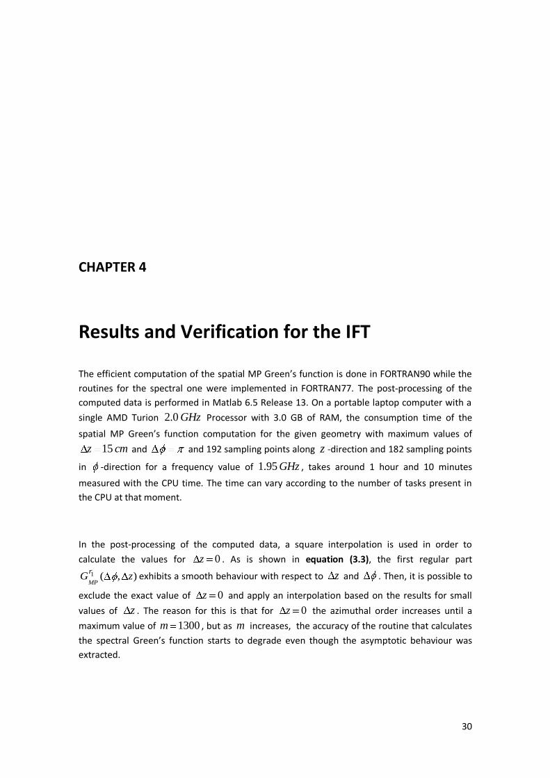
Figure 4.1.4: Equivalent surface current distribution on axially polarized patch antenna.

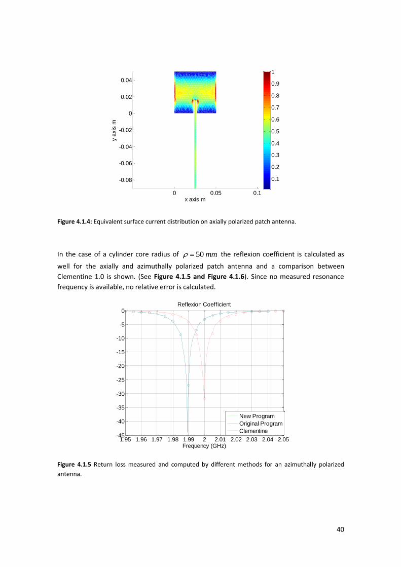
In the case of a cylinder core radius of 50 mm the reflexion coefficient is calculated as

well for the axially and azimuthally polarized patch antenna and a comparison between

Clementine 1.0 is shown. (See Figure 4.1.5 and Figure 4.1.6). Since no measured resonance

frequency is available, no relative error is calculated.

Figure 4.1.5 Return loss measured and computed by different methods for an azimuthally polarized

antenna.

0 0.05 0.1

-0.08

-0.06

-0.04

-0.02

0

0.02

0.04

x axis m

y a

xis

m

0.1

0.2

0.3

0.4

0.5

0.6

0.7

0.8

0.9

1

1.95 1.96 1.97 1.98 1.99 2 2.01 2.02 2.03 2.04 2.05-45

-40

-35

-30

-25

-20

-15

-10

-5

0Reflexion Coefficient

Frequency (GHz)

New Program

Original Program

Clementine

41

Figure 4.1.6 Return loss measured and computed by different methods for an axially polarized antenna.

1.95 1.96 1.97 1.98 1.99 2 2.01 2.02 2.03 2.04 2.05-18

-16

-14

-12

-10

-8

-6

-4

-2

0Reflexion Coefficient

Frequency (GHz)

|S1

1[d

B]|

New Program

Original Program

Clementine

42

CHAPTER 5

Numerical investigation of IFT parameters

In the calculation of the MP spatial Green’s function some parameters are introduced in order

to perform the overall computation. Recalling from the definition of the IFT in equation (2.21)

the asymptotic behaviour of the spectral Green’s function is extracted and the smoothing

parameter u is introduced and set to 14u . Furthermore, when the integration path is

deformed to avoid the surface wave poles on the real zk axis, the maximum complex distance

,max

"z

k from the real zk axis is defined (See Figure 3.1). The choice of this parameter becomes

critical for large values of z . Finally, the summation along the spectral variable m

is

truncated at 1300m but it exhibits problems as the cylinder radius ( ) increases, because

as increases, for each z step is required a large number of m to guarantee the

summation convergence and the maximum m can be reached.

5.1 Smoothing parameter u

With the short computation time achieved with the new program version, the effect of the u

parameter is investigated, starting from 1u until 40u . Though the variation of u is

introduced and removed as in equation (2.21), it seems not to influence the overall MP spatial

Green’s function regular results. Indeed, it affects as is shown in Figure 5.1.1. For small values

of u (less than one) the relative error increases quickly. It implies that u must be larger than a

certain threshold.

43

Moreover, the relative error form u 7 until u 30 has a flat characteristic that produces

stable results. Then all values of u in that region can be used.

Figure 5.1.1: Maximum relative error in and z -direction between the u variation in the new

program version and the reference value, 14u , in the original program.

On the other hand, it has to be noted that as u increases the time consumption for the MP

spatial Green’s function computation becomes larger. This happens because the numerical

convergence of the integration and summation is degraded significantly. (Figure 5.1.2). Then,

taking into account the relative error, and the consumption time, a good choice of u is 8u

which implies a total consumption time of 1 minute, 15 seconds.

Figure 5.1.2: Time consumption over different values of u .

0 5 10 15 20 25 30 35 4010

-5

10-4

10-3

u

error

rel G

A,

errorrel

GA, zz

errorrel

gV

0 5 10 15 20 25 30 35 4060

80

100

120

140

160

180

200

220

240Time variation

u

Tim

e (

sec)

44

5.2 Limits of the complex integration path

In the evaluation of the complex path integration in equation (3.2) the integral involves two

complex exponential functions as shown in equation (5.1).

(5.1) 2

1z z z zjjk z jk z jk z k ze e e e

In the square brackets, the machine must be able to differentiate between the factor one and the exponential factor when it approaches zero. This becomes critical for the extreme values

of zk and z that produce the smallest exponential value. This can be done taking into

account the smallest representable real number ( ) on the machine, in which the subroutine

is executed. zk is expressed in terms of the real and imaginary part

' "z z zk k jk

and then

equation (5.1) becomes equation (5.2).

(5.2) ' '2 " " "2 2

1 cos( ) 1 sin( ) 1z zz z z z zjk z jk z k z k z k z

e e e k z e j k z e

The maximum

"zk

for the complex path integral computation which is different from one is

determined in equation (5.3), taking into the exponential function the maximum values of zk

and z .

(5.3)

",max max

max

2

",max

ln( )

2

zk z

z

e

zk

With 0max 10z the value of "

,maxzk determined is

0

",max 0.292zk k

on a 32 bit windows

system with a double precision real data 532 . By the way, in the original program version

the value of ",maxzk

chosen is

0

",max 0.3zk k .

45

As ",maxzk

increases the overall behaviour of the program degrades and is evidently observed

as z goes up. It happens because of the machine precision is not sufficient to compute the

integral. In Figure 5.2.1-5.2.2 are shown the maximum relative error for all values of

max( ( ( , )))MPrelerror G z over z , for

0

",max 0.7zk k

and

0

",max 3.3 .zk k For the

first one, the behaviour is not seen since the difference between 0.7 and 0.3 is not so large for

the present value of max 0.15z cm . However, in the second one the effect can be

observed.

Figure 5.2.1: Maximum relative error over z

in

logarithmic scale between 0

",max 0.7zk k and

the reference 0

",max 0.3zk k .

Figure 5.2.2: Maximum relative error over z

in

logarithmic scale between 0

",max 3.3zk k and

the reference 0

",max 0.3zk k .

The maximum relative error in and z -directions max( ( ( , )))max MPrelerror G z

zis also

plotted over different values of "zk . (Figure 5.2.3). This relative error gets even worse as

"zk

increases.

0 0.2 0.4 0.6 0.8 1 1.2 1.410

-8

10-7

10-6

10-5

10-4

z/0

errorrel

GA,

errorrel

GA, zz

errorrel

gV

0 0.2 0.4 0.6 0.8 1 1.2 1.410

-8

10-6

10-4

10-2

100

102

z/0

errorrel

GA,

errorrel

GA, zz

errorrel

gV

46

Figure 5.2.3 Maximum relative error of each MP Green’s function respect to the original reference

" 0.3zk .

With the aim to improve the ",maxzk

behaviour, an automated choice of the "

,maxzk value for

the deformed complex integration path is performed. This is: If z step is lower than 0

a

fixed constant value determined by the relationship 0

" ln( )

20zk where

0max 10z

is

chosen and for larger values of z , the variation will be according to "

max

ln( )

2zk

z. (See

Equation 5.4)

(5.4)

0

0

0

",max

max

ln( ) if z <

20

ln( ) if z >

2

zk

z

The behaviour is plotted in Figure 5.2.4.

0 0.5 1 1.5 2 2.510

-6

10-5

10-4

10-3

10-2

10-1

100

k"z,max

error

rel G

A,

errorrel

GA, zz

errorrel

gV

47

Figure 5.2.4: Behaviour of "zk

over z

for a configuration with max 60z cm

and a working

frequency 1.95GHz on a 32bit windows system with

532 double precision real data.

In Figure 5.2.5 is plotted the behaviour of the spatial Mixed Potential components for a

configuration with max 90z cm using the fixed value of ",max 0.3zk . On the other hand in

Figure 5.2.6 the behaviour with the automated choice of ",maxzk

is shown. As can be noted as

z increases, especially when max 90z cm

the Im( )Vg

has a small down peak, while with

the automated choice of ",maxzk , the Im( )Vg

component exhibits a regular behaviour.

0 1 2 3 40.05

0.1

0.15

0.2

0.25

0.3

k" z, m

ax/k

0

z/0

48

Figure 5.2.5: Surface plot of the imaginary part of the total scalar potential Im( )Vg and contour plot

of the real and imaginary components of the MP spatial Green’s function.

49

Figure 5.2.6: Surface plot of the Imaginary part of the total scalar potential Im( )Vg and contour plot

of the real and imaginary components of the MP spatial Green’s function.

50

5.3 Spectral variable m

As increases, the number of spectral modes m needed increases to guarantee the

summation convergence for all values of z . Then, the maximum maxm value to truncate the

summation must be set carefully; in any case the maximum maxm will be reached for 0z .

But, this is not a problem due to in the post-processing, where the spatial Green’s function for

0z is excluded and a square interpolation is applied. The problem appears when maxm is

reached for a different z value because the result obtained is degraded since as m increases

the accuracy of the spectral Green’s function starts to degrade.

In case of max 1300m in Figure 5.3.1 is plotted the maximum m reached for the first z

different from zero, as a variation of .

Figure 5.3.1 Behaviour of max( )m with respect to the cylinder core radius, which its variation is from

25mm to 175mm. In terms of wavelength it is from 0.1667 to 1.1667 respectively.

As is shown in Figure 5.3.1 the maximum value of m is not reached, and then the value

max 1300m chosen does not affect the MP Green’s function calculations. However, in the

new program version a warning message is shown if the maxm is reached for a 0z .

20 40 60 80 100 120 140 160 180700

800

900

1000

1100

1200

1300

(cm)

max (

m)

51

CHAPTER 6

Conclusions An efficient and numerically stable spatial mixed potential Green’s function computation was

developed in the work on hand. The computation speed achieved with respect to the original

version of the software implies a time reduction of 98% . Thanks to this, it was possible to

investigate the effects of several parameters in order to improve the robustness of the overall

spatial Green’s function computation.

The most important time reduction achieved is due to the adaptive interpolation. As a

numerical result, the computation time with the adaptive interpolation applied in the original

program is around 10 minutes. This is a time reduction of 85% with respect to the original

version; the number of calls to the spectral Green’s function subroutines were reduced

significantly. The time is improved slightly more when the Filon’s integration is used instead of

the Simpson’s Rule. The computation time in this case, is reduced to around 9 minutes and 30

seconds. This is a 2.7% more reduction. The reason why the time is improved is that in the

Simpson’s rule, the zk samples, must be calculated and sought in the array of samples. When

Filon’s integration is applied the integral is solved directly and no sample determination must

be used; only the adaptive samples are needed to perform the integration.

52

Due to the calculated and stored samples, a new nesting of cycles can be done as is expressed

in Chapter 4. Re-using the samples the final time computation is 1 minute and 20 seconds. This

is an overall 98% time reduction.

The maximum relative error observed in both and z - direction, between the original and

new version, is around 410

which becomes an acceptable approximation of the exact spatial

Green’s function. Thus, when the new spatial Green’s function computation is applied in a pre-

developed method of moments software for a complex microstrip antenna printed on a

cylindrical substrate, the results in terms of the reflection coefficients and the resonance

frequency are identical.

Some parameters were introduced in order to calculate the Inverse Fourier Transform (IFT).

These are: ",maxzk

for computing the integral along the deformed complex path, the

smoothing parameter u in the regularized spectral asymptotic functions, and the maximum

azimuthal order to truncate the summation. In the ",maxzk investigation, an automatic choice of

it is done depending on the frequency and the smallest representable real number with

zero exponent on the machine. With this, the error of the machine precision as maxz

increases is eliminated. When the smoothing parameter u is analyzed in the IFT computation,

as u increases the computation time also increases. Comparing between the fixed 14u in

original program and the variation of u from 1u until 40,u a flat behaviour of the

relative error between 7u until 30u can be observed. Thus, if short computation time is

needed, a value of 8u is preferable. The computation time is reduced to 1 minute and 15

seconds with this choice. In the analysis of the maximum azimuthal order ( maxm ) needed to

truncate the summation, maxm was set to max 1300m . As increases the convergence for all

z values different from zero is achieved before maxm is reached. Thus, max 1300m is a

favorable limit.

In spite of the numerical analysis, some fields are still open for further investigations with the

aim of increasing the robustness and efficiency of the Spatial Green’s function for a circularly

cylindrical substrate. These are: the truncation value of the azimuthal order in the summation

maxm that can be set automatically by the use of a Windowing technique, and an automated

choice of u for different geometries.

REFERENCES

[1] C. M. Krowne: Cylindrical-rectangular microstrip antennas. IEEE Transactions on

Antennas and Propagation, Vol. AP-31, January 1983, pp. 194-199.

[2] J. Ashkenazy, S. Shtrikman, D. Treves: Electric surface current model for the analysis of

microstrip antennas on cylindrical bodies. IEEE Transactions on Antennas and

Propagation, Vol. AP-33, March 1985, pp. 295-300.

[3] Chen-To Tai: Dyadic Green Functions in Electromagnetic Theory. -2nd. Edition, IEEE

Press, 1994.

[4] N. G. Alexopoulos, P. L. E. Uslenghi, N. K. Uzunoglu: Microstrip dipols on cylindrical

structures. Electromagnetics 3, 1993, pp. 311-326.

[5] S. B. de Assis Fonseca, A. J. Giarola: Analysis of Microstrip Wraparound Atennas Using

Dyadic Green’s Functions. IEEE Transactions on Antennas and Propagation, Vol. AP-31,

March 1983, pp. 248-253.

[6] A. Nakatani, N. G. Alexopoulos, N. K. Uzunoglu, P.L.E Uslenghi: Accurate Green’s

function computation for printed circuit antennas on cylindrical substrates.

Electromagnetics 6, 1996, pp. 243-254.

[7] F. da Cosa Silva, S. B. de Assis Fonseca, A. J. Martins Soares, A. J. Giarola: Analysis of

microstrip antennas con circular-cylindrical substrates with a dielectric overlay. IEEE

Transactions on Antennas and Propagation, Vol. AP-39, September 1991, pp. 1398-

1403.

[8] A. Nakatani, N. G. Alexopoulos: Microstrip Elements on Cylindrical Substrates – General

Algorithm and Numerical Results. Electromagnetics 9, 1989, pp. 405-426.

[9] S. L. Cuang, L. Tsang, J. A. Kong, W.C. Chew: The equivalence of the electric and

magnetic surface current approaches in microstrip antenna studies. IEEE Transactions

on Antennas and Propagation, Vol. AP-29, January 1981, pp. 47.53.

[10] R. F. Harrington: Field Computation by Moment Methods. New York: The Macmillan

Company, 1968.

[11] J. Sun, C.-F. Wang, L.-W. Li, and M.-S Leong: Application of Kumme’s transformation in

fast computation of mixed potential Green’s function for cylindrically stratified

structure. Proc. IEEE Int. Symp. Antennas and Propag., Vol. 4, June 2003, pp. 954-957.

[12] Mixed potential spatial domain Green’s functions in fast computational form for

cylindrically stratified media. Progress in Electromagnetics Research, Vol. 45, pp. 181-

199, 2004.

[13] Further improvement for fast computation of mixed potential Green’s function for

cylindrical stratified media. IEEE Transactions on Antennas and Propagation, Vol. 52,

no. 11, pp. 3026-3036, Nov. 2004.

[14] T. Bertuch: Full-wave analysis of cylindrical conformal microstrip antennas with

electromagnetically coupled feeding. Germany, Nov. 1996.

[15] G. Vecchi, T. Bertuch and M. Orefice: Spectral-domain analysis of printed antennas of

general shape on cylindrical substrates. Proc. IEEE Int. Symp. Antennas and Propag, vol.

3, June 1997, pp. 1496-1499.

[16] Analysis of cylindrical antennas with sub sectional basis functions in the spectral

domain. Proc. Int. Conf. Electromag. Adv. Appl. (ICEAA), Sep. 1997, pp. 301-304.

[17] T. Bertuch, G. Vecchi, L. Matekovits, and M. Orefice: Full-wave analysis of conformal

antennas on arbitrary shapes printed on circular cylinder. Proc. 1st European workshop

on Conformal Antennas, Oct. 1999, pp. 8-11.

[18] T. Bertuch, G. Vecchi, and M. Orefice: Efficient spectral-domain simulation of

conformal antennas of arbitrary shapes printed on circular cylinders. Proc. Millenium

Conf. Antennas and Propagat. (AP2000), April 2000.

[19] R. F. Harrington: Time-Harmonic Electromagnetic Fields. New York: The McGraw-Hill,

1961

[20] R. C. Hall, C. H. Thng, and D. C. Chang: Mixed potential Green’s functions for cylindrical

microstrip structures. Proc. IEEE Int. Symp. Antenans and Propag., Vol. 4, June 1995,

pp. 1776-1779.

[21] S. Singh, W. F. Richards, J. R. Zinecker, and D R. Wilton: Accelerating the convergence of

series representing the free space periodic Green’s function. IEEE Trans. Antennas

Propag., Vol. 38, no. 12, pp. 1958-1962, Dec. 1990.

[22] M. Abramowitz, I. A. Stegun: Handbook of mathematical functions. 9th edition, New

York, Dover Publications, 1972.

APPENDIX A

Method of moments The Integral Equation (IE) solved applying the Method of Moments (MoM) formulation, is determined by replacing the printed metallizations with unknown equivalent surface currents

sJ . Thus, the total electric field at the position r is expressed by the sum of the so-called

impressed ( )iE r and scattered { }ssE J fields produced by equivalent point sources at the

position 'r (See Equation 1).

(1) ( ) ( ) { ( ')}i ssE r E r E J r

Since the electric field tangential tanE at the position of the metallizations is zero, equation (1)

becomes equation (2), where the second term in equation (2) is expressed by the convolution

between the Green’s function ( , ')G r r and ( ')sJ r on the replaced conductors’area 'A (See

equation 3).

(2) tan tan( ) { } 0i ssE r E J

(3) tan

ˆ{ } ( , '). ( ') 'ss sE J n G r r J r dA

In a more compact form, equation (2) is written as equation (4), where L is the linear integral

operator.

(4) tan ( ) { }isE r L J

The unknown equivalent surface currents is approximated by a set of so-called basis functions bqJ with {1,2, , }q Q and initially unknown coefficients q (see equation (5)).

(5) 1

Qb

s q qq

J J

To calculate the coefficients q , a set of testing functions tpJ with {1,2, , }p P , is used.

These, are defined in the same domain as the basis functions, applying Galerkin’s method

( p q ). Thus, the complete system to be solved is written in equation (6), where equation

(5) is used in equation (4).

(6) tan

1

, { } , ( )Q

t b t iq p p p

q

J L J J E r

Equation (6) is written in matrix form as

Z V

Where,

tan

[ , ] , { }

[ ]

[ ] , ( )

q

t bp p

t ip

Z p q J L J

q

V p J E r

Z is called impedance matrix, in which its components are the reaction integrals between the

testing function and the scattered electric field. The coefficients q of the approximation of

the current distribution are determined solving the linear system.

APPENDIX B

Filon’s integration

The integral to be solved is:

(1)

0

( )( , )cos( )

d

restz z zMPk k

G m k k z dk

The term ( )

( , )rest

zMPG m k

is described with the common form of a linear equation

1 1( )sy y m x x , where 2 1

2 1

s

y ym

x x

is the slope and 1x and

2x are the zk samples at

the boundaries of the interval; 1y and

2y are the evaluated spectral Green’s function

components for the zk samples respectively. Then, the integral is divided in short intervals and

a summation over them is done equation (2).

(2)

1 1

,

, 1

( ) cos( ) 2,3...

total number of samples

z i

z i

k

z z zki

sy m k x k z dk i n

n

Since in equation (2) the terms1y ,

2y , sm

are constants, the integral is solved in this way:

(3) 1 1

, ,

, 1 , 1

,

, 1

cos( ) cos( ) cos( )z i z i

z i z i

z i

z i

k k k

z z s z z z z zk k ky k z dk m k k z dk x k z dk

The first and third integrals are solved easily because the kernel of them implies only the

integration of a cosine function. The second one is solved by the parts formula

udv uv vdu :

(4)

2

, , 1, , 1

, , 1

,

, 1

cos( ) sin( ) sin( )

1 cos( ) cos( )

z i z iz z z z i z i

z i z i

z i

z i

k

k

kkk k z dk k z k z

z z

k z k zz

Then, the final result of the integral is shown in equation (5).

(5)

1 1

2

,

, 1

1, , 1

, , 1

( ) cos( ) sin( ) sin( )

cos( ) cos( )

2,3...

to

i

z i

z i

ki i

s z z z z i z ik

sz i z i

yyy m k x k z dk k z k z

z z

mk z k z

z

i n

n tal number of samples