efficient max-margin multi-label classification with applications to

Mach Learn manuscript No.(will be inserted by the editor)

Efficient Max-Margin Multi-Label Classification with

Applications to Zero-Shot Learning

Bharath Hariharan · S. V. N. Vishwanathan ·

Manik Varma

Received: 30 September 2010 / Accepted: date

Abstract The goal in multi-label classification is to tag a data point with the subset

of relevant labels from a pre-specified set. Given a set of L labels, a data point can

be tagged with any of the 2L possible subsets. The main challenge therefore lies in

optimising over this exponentially large label space subject to label correlations.

Our objective, in this paper, is to design efficient algorithms for multi-label clas-

sification when the labels are densely correlated. In particular, we are interested in

the zero-shot learning scenario where the label correlations on the training set might

be significantly different from those on the test set.

We propose a max-margin formulation where we model prior label correlations

but do not incorporate pairwise label interaction terms in the prediction function. We

show that the problem complexity can be reduced from exponential to linear while

modelling dense pairwise prior label correlations. By incorporating relevant corre-

lation priors we can handle mismatches between the training and test set statistics.

Our proposed formulation generalises the effective 1-vs-All method and we provide

a principled interpretation of the 1-vs-All technique.

We develop efficient optimisation algorithms for our proposed formulation. We

adapt the Sequential Minimal Optimisation (SMO) algorithm to multi-label classifi-

cation and show that, with some book-keeping, we can reduce the training time from

being super-quadratic to almost linear in the number of labels. Furthermore, by ef-

fectively re-utilizing the kernel cache and jointly optimising over all variables, we

can be orders of magnitude faster than the competing state-of-the-art algorithms. We

B. Hariharan

University of California at Berkeley

E-mail: [email protected]

S. V. N. Vishwanathan

Purdue University


Manik Varma

Microsoft Research India


2 Bharath Hariharan et al.

also design a specialised algorithm for linear kernels based on dual co-ordinate ascent

with shrinkage that lets us effortlessly train on a million points with a hundred labels.

1 Introduction

Our objective, in this paper, is to develop efficient algorithms for max-margin, multi-

label classification. Given a set of pre-specified labels and a data point, (binary) multi-

label classification deals with the problem of predicting the subset of labels most rel-

evant to the data point. This is in contrast to multi-class classification where one has

to predict just the single, most probable label. For instance, rather than simply saying

that Fig. 1 is an image of a Babirusa we might prefer to describe it as containing a

brown, hairless, herbivorous, medium sized quadruped with tusks growing out of its

snout.

Fig. 1 Having never seen a Babirusa before we can still describe it as a brown, hairless, herbivorous,

medium sized quadruped with tusks growing out of its snout.

There are many advantages in generating such a description and multi-label clas-

sification has found applications in areas ranging from computer vision to natural

language processing to bio-informatics. We are specifically interested in the problem

of image search on the web and in personal photo collections. In such applications,

it is very difficult to get training data for every possible object out there in the world

that someone might conceivably search for. In fact, we might not have any training

images whatsoever for many object categories such as the obscure Babirusa. Never-

theless, we can not preclude the possibility of someone searching for one of these

objects. A similar problem is encountered when trying to search videos on the basis

of human body pose and motion and many other applications such as neural activity

decoding (Palatucci et al., 2009).

One way of recognising object instances from previously unseen test categories

(the zero-shot learning problem) is by leveraging knowledge about common attributes

Efficient Max-Margin Multi-Label Classification with Applications to Zero-Shot Learning 3

and shared parts. For instance, given adequately labelled training data, one can learn

classifiers for the attributes occurring in the training object categories. These classi-

fiers can then be used to recognise the same attributes in object instances from the

novel test categories. Recognition can then proceed on the basis of these learnt at-

tributes (Farhadi et al., 2009, 2010; Lampert et al., 2009).

The learning problem can therefore be posed as multi-label classification where

there is a significant difference between attribute (label) correlations in the training

categories and the previously unseen test categories. What adds to the complexity of

the problem is the fact that these attributes are often densely correlated as they are

shared across most categories. This makes optimising over the exponentially large

output space, given by the power set of all labels, very difficult. The problem is acute

not just during prediction but also during training as the number of training images

might grow to be quite large over time in some applications.

Previously proposed solutions to the multi-label problem take one of two ap-

proaches – neither of which can be applied straight forwardly in our scenario. In the

first, labels are a priori assumed not to be correlated so that a predictor can be trained

for each label independently. This reduces training and prediction complexity from

exponential in the number of labels to linear. Such methods can therefore scale effi-

ciently to large problems but at the cost of not being able to model label correlations.

Furthermore, these methods typically tend not to minimise a multi-label loss. In the

second, label correlations are explicitly taken into account by incorporating pairwise,

or higher order, label interactions. However, exact inference is mostly intractable for

densely correlated labels and in situations where the label correlation graph has loops.

Most approaches therefore assume sparsely correlated labels such as those arranged

in a hierarchical tree structure.

In this paper, we follow a middle approach. We develop a max-margin multi-

label classification formulation, referred to as M3L, where we do model prior label

correlations but do not incorporate pairwise, or higher order, label interaction terms

in the prediction function. This lets us generalise to the case where the training label

correlations might differ significantly from the test label correlations. We can also

efficiently handle densely correlated labels. In particular, we show that under fairly

general assumptions of linearity, the M3L primal formulation can be reduced from

having an exponential number of constraints to linear in the number of labels. Fur-

thermore, if no prior information about label correlations is provided, M3L reduces

directly to the 1-vs-All method. This lets us provide a principled interpretation of the

1-vs-All multi-label approach which has enjoyed the reputation of being a popular,

effective but nevertheless, heuristic technique.

Much of the focus of this paper is on optimising the M3L formulation. It turns out

that it is not good enough to just reduce the primal to have only a linear number of

constraints. A straight forward application of state-of-the-art decompositional optimi-

sation methods, such as Sequential Minimal Optimisation (SMO), would lead to an

algorithm that is super-quadratic in the number of labels. We therefore develop spe-

cialised optimisation algorithms that can be orders of magnitude faster than compet-

ing methods. In particular, for kernelised M3L, we show that by simple book keeping

and delaying gradient updates, SMO can be adapted to yield a linear time algorithm.

Furthermore, due to efficient kernel caching and jointly optimising all variables, we


can sometimes be an order of magnitude faster than the 1-vs-All method. Thus our

code, available from (Hariharan et al., 2010a), should also be very useful for learning

independent 1-vs-All classifiers. For linear M3L, we adopt a dual co-ordinate ascent

strategy with shrinkage which lets us efficiently tackle large scale training data sets.

In terms of prediction accuracy, we show that incorporating prior knowledge about

label correlations using the M3L formulation can substantially boost performance

over independent methods.

The rest of the paper is organised as follows. Related work is reviewed in Sec-

tion 2. Section 3 develops the M3L primal formulation and shows how to reduce the

number of primal constraints from exponential to linear. The 1-vs-All formulation

is also shown to be a special case of the M3L formulation. The M3L dual is devel-

oped in Section 4 and optimised in Section 5. We develop algorithms tuned to both

the kernelised and the linear case. Experiments are carried out in Section 7 and it

is demonstrated that the M3L formulation can lead to significant gains in terms of

both optimisation and prediction accuracy. An earlier version of the paper appeared

in (Hariharan et al., 2010b).

2 Related Work

The multi-label problem has many facets including binary (Tsoumakas & Katakis,

2007; Ueda & Saito, 2003), multi-class (Dekel & Shamir, 2010) and ordinal (Cheng et al.,

2010) multi-label classification as well as semi-supervised learning, feature selec-

tion (Zhang & Wang, 2009b), active learning (Li et al., 2004), multi-instance learn-

ing (Zhang & Wang, 2009a), etc. Our focus, in this paper, is on binary multi-label

classification where most of the previous work can be categorised into one of two

approaches depending on whether labels are assumed to be independent or not. We

first review approaches that do assume label independence. Most of these methods

try and reduce the multi-label problem to a more “canonical” one such as regression,

ranking, multi-class or binary classification.

In regression methods (Hsu et al., 2009; Ji et al., 2008; Tsoumakas & Katakis,

2007), the label space is mapped onto a vector space (which might sometimes be

a shared subspace of the feature space) where regression techniques can be applied

straightforwardly. The primary advantage of such methods is that they can be ex-

tremely efficient if the mapped label space has significantly lower dimensionality

than the original label space (Hsu et al., 2009). The disadvantage of such approaches

is that the choice of an appropriate mapping might be unclear. As a result, minimis-

ing regression loss functions, such as square loss, in this space might be very efficient

but might not be strongly correlated with minimising the desired multi-label loss.

Furthermore, classification involves inverting the map which might not be straight-

forward, result in multiple solutions and might involve heuristics.

A multi-label problem with L labels can be viewed as a classification problem

with 2L classes (McCallum, 1999; Boutell et al., 2004) and standard multi-class tech-

niques can be brought to bear. Such an approach was shown to give the best empiri-

cal results in the survey by (Tsoumakas & Katakis, 2007). However, such approaches

have three major drawbacks. First, since not all 2L label combinations can be present


in the training data, many of the classes will have no positive examples. Thus, pre-

dictors can not be learnt for these classes implying that these label combinations can

not be recognised at run time. Second, the 0/1 multi-class loss optimised by such

methods forms a poor approximation to most multi-label losses. For instance, the 0/1

loss would charge the same penalty for predicting all but one of the labels correctly

as it would for predicting all of the labels incorrectly. Finally, learning and predicting

with such a large number of classifiers might be very computationally expensive.

Binary classification can be leveraged by replicating the feature vector for each

data point L times. For copy number l, an extra dimension is added to the feature vec-

tor with value l and the training label is +1 if label l is present in the label set of the

original point and −1 otherwise. A binary classifier can be learnt from this expanded

training set and a novel point classified by first replicating it as described above and

then applying the binary classifier L times to determine which labels are selected.

Due to the data replication, applying a binary classifier naively would be computa-

tionally costly and would require that complex decision boundaries be learnt. How-

ever, (Schapire & Singer, 2000) show that the problem can be solved efficiently using

Boosting. A somewhat related technique is 1-vs-All (Rifkin & Khautau, 2004) which

independently learns a binary classifier for each label. As we’ll show in Section 3,

our formulation generalises 1-vs-All to handle prior label correlations.

A ranking based solution was proposed in (Elisseeff & Weston, 2001). The ob-

jective was to ensure that, for every data point, all the relevant labels were ranked

higher than any of the irrelevant ones. This approach has been influential but suffers

from the drawback of not being able to easily determine the number of labels to se-

lect in the ranking. The solution proposed in (Elisseeff & Weston, 2001) was to find

a threshold so that all labels scoring above the threshold were selected. The thresh-

old was determined using a regressor trained subsequently on the ranker output on

the training set. Many variations have been proposed, such as using dummy labels

to determine the threshold, but each has its own limitations and no clear choice has

emerged. Furthermore, posing the problem as ranking induces a quadratic number of

constraints per example which leads to a harder optimisation problem. This is ame-

liorated in (Crammer & Singer, 2003) who reduced the space complexity to linear

and time complexity to sub-quadratic.

Most of the approaches mentioned above do not explicitly model label correla-

tions – (McCallum, 1999) has a generative model which can, in principle, handle cor-

relations but greedy heuristics are used to search over the exponential label space. In

terms of discriminative methods, most work has focused on hierarchical tree, or for-

est, structured labels. Methods such as (Cai & Hofmann, 2007; Cesa-Bianchi et al.,

2006) optimise a hierarchical loss over the tree structure but do not incorporate

pairwise, or higher order, label interaction terms. In both these methods, a label is

predicted only if its parent has also been predicted in the hierarchy. For instance,

(Cesa-Bianchi et al., 2006) train a classifier for each node of the tree. The positive

training data for the classifier is the set of data points marked with the node label

while the negative training points are selected from the sibling nodes. Classification

starts at the root and all the children classifiers are tested to determine which path to

take. This leads to a very efficient algorithm during both training and prediction as

each classifier is trained on only a subset of the data. Alternatively, (Cai & Hofmann,


2007) classify at only the leaf nodes and use them as a proxy for the entire path

starting from the root. A hierarchical loss is defined and optimised using the ranking

method of (Elisseeff & Weston, 2001).

The M3N formulation of (Taskar et al., 2003) was the first to suggest max-margin

learning of label interactions. The original formulation starts off having an exponen-

tial number of constraints. These can be reduced to quadratic if the label interactions

formed a tree or forest. Approximate algorithms are also developed for sparse, loopy

graph structures. While the M3N formulation dealt with the Hamming loss, a more

suitable hierarchical loss was introduced and efficiently optimised in (Rousu et al.,

2006) for the case of hierarchies. Note that even though these methods take label cor-

relations explicitly into account, they are unsuitable for our purposes as they cannot

handle densely correlated labels and learn training set label correlations which are

not useful at test time since the statistics might have changed significantly.

Finally, (Tsochantaridis et al., 2005) propose an iterative, cutting plane algorithm

for learning in general structured output spaces. The algorithm adds the worst vio-

lating constraint to the active set in each iteration and is proved to take a maximum

number of iterations independent of the size of the output space. While this algorithm

can be used to learn pairwise label interactions it too can’t handle a fully connected

graph as the worst violating constraint cannot be generally found in polynomial time.

However, it can be used to learn our proposed M3L formulation but is an order of

magnitude slower than the specialised optimisation algorithms we develop.

Zero shot learning deals with the problem of recognising instances from novel

categories that were not present during training. It is a nascent research problem and

most approaches tackle it by building an intermediate representation leveraging at-

tributes, features or classifier outputs which can be learnt from the available training

data (Farhadi et al., 2009, 2010; Lampert et al., 2009; Palatucci et al., 2009). Novel

instances are classified by first generating their intermediate representation and then

mapping it onto the novel category representation (which can be generated using

meta-data alone). The focus of research has mainly been on what is a good interme-

diate level representation and how should the mapping be carried out.

A popular choice of the intermediate level representation have been parts and

attributes – whether they be semantic or discriminative. Since not all features are rel-

evant to all attributes, (Farhadi et al., 2009) explore feature selection so as to better

predict a novel instance’s attributes. Probabilistic techniques for mapping the list of

predicted attributes to a novel category’s list of attributes (known a priori) are de-

veloped in (Lampert et al., 2009) while (Palatucci et al., 2009) carry out a theoretical

analysis and use the one nearest neighbour rule. An alternative approach to zero-shot

learning is not to name the novel object, or explicitly recognise its attributes, but

simply say that it is “like” an object seen during training (Wang et al., 2010). For in-

stance, the Babirusa in Fig 1 could be declared to be like a pig. This is sufficient for

some applications and works well if the training set has good category level coverage.


3 M3L: The Max-Margin Multi-Label Classification Primal Formulation

The objective in multi-label classification is to learn a function f which can be used

to assign a set of labels to a point x. We assume thatN training data points have been

provided of the form (xi,yi) ∈ RD × {±1}L with yil being +1 if label l has been

assigned to point i and −1 otherwise. Note that such an encoding allows us to learn

from both the presence and absence of labels, since both can be informative when

predicting test categories.

A principled way of formulating the problem would be to take the loss function

∆ that one truly cares about and minimise it over the training set subject to regulari-

sation or prior knowledge. Of course, since direct minimisation of most discrete loss

functions is hard, we might end up minimising an upper bound on the loss, such as

the hinge. The learning problem can then be formulated as the following primal

P1 = minf

1

2‖f‖2 + C

N∑

i=1

ξi (1)

s. t. f(xi,yi) ≥ f(xi,y) +∆(yi,y)− ξi ∀i,y ∈ {±1}L \ {yi} (2)

ξi ≥ 0 ∀i (3)

with a new point x being assigned labels according to y∗ = argmaxy f(x,y). The

drawback of such a formulation is that there are N2L constraints which make direct

optimisation very slow. Furthermore, classification of novel points might require 2L

function evaluations (one for each possible value of y), which can be prohibitive at

run time. In this Section, we demonstrate that, under general assumptions of linearity,

(P1) can be reformulated as the minimisation of L densely correlated sub-problems

each having only N constraints. At the same time, prediction cost is reduced to a

single function evaluation with complexity linear in the number of labels. The ideas

underlying this decomposition were also used in (Evgeniou et al., 2005) in a multi-

task learning scenario. However, their objective is to combine multiple tasks into a

single learning problem, while we are interested in decomposing (3) into multiple

subproblems.

We start by making the standard assumption that

f(x,y) = wt(φ(x)⊗ψ(y)) (4)

where φ and ψ are the feature and label space mappings respectively, ⊗ is the Kro-

necker product and wt denotes w transpose. Note that, for zero shot learning, it is

possible to theoretically show that , in the limit of infinite data, one does not need to

model label correlations when training and test distributions are the same (Palatucci et al.,

2009). In practice, however, training sets are finite, often relatively small, and have

label distributions that are significantly different from the test set. Therefore to incor-

porate prior knowledge and correlate classifiers efficiently, we assume that labels have

at most linear, possibly dense, correlation so that it is sufficient to chooseψ(y) = Py

where P is an invertible matrix encoding all our prior knowledge about the labels. If

we assume f to be quadratic (or higher order) in y, as is done in structured output


prediction, then it would not be possible to reduce the number of constraints from ex-

ponential to linear while still modelling dense, possibly negative, label correlations.

Furthermore, learning label correlation on the training set by incorporating quadratic

terms in y might not be fruitful as the test categories will have very different corre-

lation statistics. Thus, by sacrificing some expressive power, we hope to build much

more efficient algorithms that can still give improved prediction accuracy in the zero-

shot learning scenario.

We make another standard assumption that the the chosen loss function should

decompose over the individual labels (Taskar et al., 2003). Hence, we require that

∆(yi,y) =

L∑

l=1

∆l(yi, yl) (5)

where yl ∈ {±1} corresponds to label l in the set of labels represented by y. For in-

stance, the popular Hamming loss, amongst others, satisfies this condition. We define

the Hamming loss∆H(yi,y), between a ground truth label yi and a prediction y as

∆H(yi,y) = yti(yi − y) (6)

which is a count of twice the total number of individual labels mispredicted in y. Note

that the Hamming loss can be decomposed over the labels as ∆H(yi,y) =∑

l 1 −ylyil. Of course, for ∆ to represent a sensible loss we also require that ∆(yi,y) ≥∆(yi,yi) = 0.

Under these assumptions, (P1) can be expressed as

P1 ≡ minw

1

2wtw + C

N∑

i=1

maxy∈{±1}L

[∆(yi,y) +wtφ(xi)⊗P(y − yi)] (7)

where the constraints have been moved into the objective and ξi ≥ 0 eliminated by

including y = yi in the maximisation. To simplify notation, we express the vectorw

as a D × L matrixW so that

P1 ≡ minW

1

2Trace(WtW)+C

N∑

i=1

maxy∈{±1}L

[∆(yi,y)+(y−yi)tPtWtφ(xi)]

(8)

Substituting Z = WP, R = PtP ≻ 0 and using the identity Trace(ABC) =Trace(CAB) results in

P1 ≡ minZ

1

2

L∑

l=1

L∑

k=1

R−1

lk ztlzk+

C

N∑

i=1

maxy∈{±1}L

[

L∑

l=1

[∆l(yi, yl) + (yl − yil)ztlφ(xi)]

]

(9)


where zl is the lth column of Z. Note that the terms inside the maximisation break

up independently over the L components of y. It is therefore possible to interchange

the maximisation and summation to get

P1 ≡ minZ

1

2

L∑

l=1

L∑

k=1

R−1

lk ztlzk+

C

N∑

i=1

L∑

l=1

[

maxyl∈{±1}

[∆l(yi, yl) + (yl − yil)ztlφ(xi)]

]

(10)

This leads to an equivalent primal formulation (P2) as the summation of L correlated

problems, each having N constraints which is significantly easier to optimise.

P2 =

L∑

l=1

Sl (11)

Sl = minZ,ξ

1

2ztl

L∑

k=1

R−1

lk zk + CN∑

i=1

ξil (12)

s. t. 2yilztlφ(xi) ≥ ∆l(yi,−yil)− ξil (13)

ξil ≥ ∆l(yi, yil) (14)

Furthermore, a novel point x can be assigned the set of labels for which the entries of

sign(Ztφ(x)) are +1. This corresponds to a single evaluation of f taking time linear

in the number of labels.

The L classifiers in Z are not independent but correlated by R – a positive def-

inite matrix encoding our prior knowledge about label correlations. One might typi-

cally have thought of learning R from training data. For instance, one could learn R

directly or expressR−1 as a linear combination of predefined positive definite matri-

ces with learnt coefficients. Such formulations have been developed in the Multiple

Kernel Learning literature and we could leverage some of the proposed MKL opti-

mization techniques (Vishwanathan et al., 2010). However, in the zero-shot learning

scenario, learning R from training data is not helpful as the correlations between

labels during training might be significantly different from those during testing.

Instead, we rely on the standard zero-shot learning assumption, that the test cat-

egory attributes are known a priori (Farhadi et al., 2009, 2010; Lampert et al., 2009;

Palatucci et al., 2009). Furthermore, if the prior distribution of test categories was

known, then R could be set to approximate the average pairwise test label correlation

(see Section 7.2.1 for details).

Note that, in the zero-shot learning scenario, R can be dense, as almost all the

attributes might be shared across categories and correlated with each other, and can

also have negative entries representing negative label correlations. We propose to im-

prove prediction accuracy on the novel test categories by encoding prior knowledge

about their label correlations inR.

Note that we deliberately chose not to include bias terms b in f even though the

reduction from (P1) to (P2) would still have gone through and the resulting kernelised


optimisation been more or less the same (see Section 7.1). However, we would then

have had to regularise b and correlate it usingR. Otherwise bwould have been a free

parameter capable of undoing the effects ofR on Z. Therefore, rather than explicitly

have b and regularise it, we implicitly simulate b by adding an extra dimension to

the feature vector. This has the same effect while keeping optimisation simple.

We briefly discuss two special cases before turning to the dual and its optimisa-

tion.

3.1 The Special Case of 1-vs-All

If label correlation information is not included, i. e. R = I, then (P2) decouples into

L completely independent sub-problems each of which can be tackled in isolation. In

particular, for the Hamming loss we get

P3 =

L∑

l=1

Sl (15)

Sl = minzl,ξ

1

2ztlzl + 2C

N∑

i=1

ξi (16)

s. t. yilztlφ(xi) ≥ 1− ξi (17)

ξi ≥ 0 (18)

Thus, Sl reduces to an independent binary classification sub-problem where the pos-

itive class contains all training points tagged with label l and the negative class con-

tains all other points. This is exactly the strategy used in the popular and effective

1-vs-All method and we can therefore now make explicit the assumptions underly-

ing this technique. The only difference is that one should charge a misclassification

penalty of 2C to be consistent with the original primal formulation.

3.2 Relating the Kernel to the Loss

In general, the kernel is chosen so as to ensure that the training data points become

well separated in the feature space. This is true for both Kx, the kernel on x, as well

as Ky , the kernel on y. However, one might also take the view that since the loss ∆induces a measure of dissimilarity in the label space it must be related to the kernel

on y which is a measure of similarity in the label space. This heavily constrains

the choice of Ky and therefore the label space mapping ψ. For instance, if a linear

relationship is assumed, we might choose∆(yi,y) = Ky(yi,yi)−Ky(yi,y). Notethat this allows ∆ to be asymmetric even though Ky is not and ensures the linearity

of ∆ if ψ, the label space mapping, is linear.

In this case, label correlation information should be encoded directly into the loss.

For example, the Hamming loss could be transformed to∆H(yi,y) = ytiR(yi−y).

R is the same matrix as before except the interpretation now is that the entries of

R encode label correlations by specifying the penalties to be charged if a label is


misclassified in the set. Of course, for∆ to be a valid loss, not only mustR be positive

definite as before but it now must also be diagonally dominant. As such, it can only

encode “weak” correlations. Given the choice of ∆ and the linear relationship with

Ky , the label space mapping gets fixed to ψ(y) = Py where R = PtP.

Under these assumptions once can still go from (P1) to (P2) using the same

steps as before. The main differences are that R is now more restricted and that

∆l(yi, yl) = (1/L)ytiRyi − yly

tiRl where Rl is the l

th column of R. While this

result is theoretically interesting, we do not explore it further in this paper.

4 The M3L Dual Formulation

The dual of (P2) has similar properties in that it can be viewed as the maximisation

of L related problems which decouple into independent binary SVM classification

problems whenR = I. The dual is easily derived if we rewrite (P2) in vector notation.

Defining

Yl = diag([y1l, . . . , yNl]) (19)

Kx = φt(X)φ(X) (20)

∆±l = [∆l(y1,±y1l), . . . , ∆l(yN ,±yNl)]

t (21)

we get the following Lagrangian

L =L∑

l=1

( 12

L∑

k=1

R−1

lk ztlzk + C1tξl − βtl(ξl −∆+

l )

−αtl(2Ylφ

t(X)zl −∆−l + ξl)) (22)

with the optimality conditions being

∇zlL = 0 ⇒

L∑

k=1

R−1

lk zk = 2φ(X)Ylαl (23)

∇ξlL = 0 ⇒ C1−αl − βl = 0 (24)

Substituting these back into the Lagrangian leads to the following dual

D2 = max0≤α≤C1

L∑

l=1

αtl(∆

−l −∆+

l )− 2

L∑

l=1

L∑

k=1

RlkαtlYlKxYkαk (25)

Henceforth we will drop the subscript on the kernel matrix and writeKx as K.


5 Optimisation

The M3L dual is similar to the standard SVM dual. Existing optimisation techniques

can therefore be brought to bear. However, the dense structure of R couples all NLdual variables and simply porting existing solutions leads to very inefficient code. We

show that, with book keeping, we can easily go from an O(L2) algorithm to an O(L)algorithm. Furthermore, by re-utilising the kernel cache, our algorithms can be very

efficient even for non-linear problems. We treat the kernelised and linear M3L cases

separately.

5.1 Kernelised M3L

The Dual (D2) is a convex quadratic programme with very simple box constraints.

We can therefore use co-ordinate ascent algorithms (Platt, 1999; Fan et al., 2005;

Lin et al., 2009) to maximise the dual. The algorithms start by picking a feasible

point – typically α = 0. Next,two variables are selected and optimised analytically.

This step is repeated until the projected gradient magnitude falls below a threshold

and the algorithm can be shown to have converged to the global optimum (Lin et al.,

2009). The three key components are therefore: (a) reduced variable optimisation; (b)

working set selection and (c) stopping criterion and kernel caching. We now discuss

each of these components. The pseudo-code of the algorithm and proof of conver-

gence are given in the Appendix.

5.1.1 Reduced Variable Optimisation

If all but two of the dual variables were fixed, say αpl and αql along the label l, thenthe dual optimisation problem reduces to

D2pql = maxδpl,δql

− 2(δ2plKppRll + δ2qlKqqRll + 2δplδqlyplyqlKpqRll)

+ δplgpl + δqlgql (26)

s. t.− αpl ≤ δpl ≤ C − αpl (27)

− αql ≤ δql ≤ C − αql (28)

where δpl = αnewpl − αoldpl and δql = αnewql − αoldql and

gpl = ∇αplD2 = ∆−

pl −∆+

pl − 4N∑

i=1

L∑

k=1

RklKipyikyplαik (29)

Note that D2pql has a quadratic objective in two variables which can be max-

imised analytically due to the simple box constraints. We do not give the expressions

for αnewpl and αnewql which maximise D2pql as many special cases are involved for

when the variables are at bound but they can be found in Algorithm 2 of the pseudo-

code in Appendix A.


5.1.2 Working Set Selection

Since the M3L formulation does not have a bias term, it can be optimized by picking

a single variable at each iteration rather than a pair of variables. This leads to a low

cost per iteration but a large number of iterations. Selecting two variables per iteration

increases the cost per iteration but significantly reduces the number of iterations as

second order information can be incorporated into the variable selection policy.

If we were to choose two variables to optimise along the same label l, say αpl and

αql, then the maximum change that we could affect in the dual is given by

δD2(αpl, αql) =g2plKqq + g2qlKpp − 2gplgqlyplyqlKpq

8Rll(KppKqq −K2pq)

(30)

In terms of working set selection, it would have been ideal to have chosen the two

variables αpl and αql which would have maximised the increase in the dual objective.

However, this turns out to be too expensive in practice. A good approximation is

to choose the first point αpl to be the one having the maximum projected gradient

magnitude. The projected gradient is defined as

gpl =

gpl if αpl ∈ (0, C)min(0, gpl) if αpl = Cmax(0, gpl) if αpl = 0

(31)

and hence the first point is chosen as

(p∗, l∗) = argmaxp,l

|gpl| (32)

Having chosen the first point, the second point is chosen to be the one that maximises

(30).

Working set selection can be made efficient by maintaining the set of gradients g.Every time a variable, say αpl is changed, the gradients need to be updated as

gnewjk = goldjk − 4yplyjkRklKpj(αnewpl − αoldpl ) (33)

Note that because of the dense structure of R all NL gradients have to be updated

even if a single variable is changed. Since there are NL variables and each has to be

updated presumably at least once we end up with an algorithm that takes time at least

N2L2.

The algorithm can be made much more efficient if, with some book keeping, not

all gradients had to be updated every time a variable was changed. For instance, if we

were to fix a label l and modify L variables along the chosen label, then the gradient

update equations could be written as

gnewjk = goldjk − 4yjk

N∑

i=1

yilRklKij(αnewil − αoldil ) (34)

= goldjk − 4Rklyjkujl (35)


where ujl =

N∑

i=1

Kijyil(αnewil − αoldil ) (36)

As long as we are changing variables along a particular label, the gradient updates

can be accumulated in u and only when we switch to a new variable do all the gradi-

ents have to be updated. We therefore end up doing O(NL) work after changing Lvariables resulting in an algorithm which takes time O(N2L) rather than O(N2L2).

5.1.3 Stopping Criterion and Kernel Caching

We use the standard stopping criterion that the projected gradient magnitude for all

NL dual variables should be less than a predetermined threshold.

We employ a standard Least Recently Used (LRU) kernel cache strategy imple-

mented as a circular queue. Since we are optimising over all labels jointly, the kernel

cache gets effectively re-utilised, particularly as compared to independent methods

that optimise one label at a time. In the extreme case, independent methods will have

to rebuild the cache for each label which can slow them down significantly.

6 Linear M3L

We build on top of the stochastic dual coordinate ascent with shrinkage algorithm

of (Hsieh et al., 2008). At each iteration, a single dual variable is chosen uniformly at

random from the active set, and optimised analytically. The variable update equation

is given by

αnewpl = max(0,min(C,αoldpl + δαpl)) (37)

where δαpl =∆−

pl −∆+

pl − 4∑

q

∑

kKpqRlkyplyqkαqk

4KppRll

(38)

=∆−

pl −∆+

pl − 2yplztlxp

4Rllxtpxp

(39)

As can be seen, the dual variable update can be computed more efficiently in terms of

the primal variables Z which then need to be maintained every time a dual variable is

modified. The update equation for Z every time αpl is modified is

znewl = zoldl + 2Rklypl(αnewpl − αoldpl )xp (40)

Thus, all the primal variables Z need to be updated every time a single dual variable

is modified. Again, as in the kernelised case, the algorithm can be made much more

efficient by fixing a label l and modifying L dual variables along it while delaying

the gradient updates as

znewk = zoldk + 2Rkl

N∑

j=1

yjl(αnewjl − αoldjl )xj (41)


= zoldk + 2Rklvl (42)

where vl =

N∑

j=1

yjl(αnewjl − αoldjl )xj (43)

In practice, it was observed that performing L stochastic updates along a chosen label

right from the start could slow down convergence in some cases. Therefore, we ini-

tially use the more expensive strategy of choosing dual variables uniformly at random

and only after the projected gradient magnitudes are below a pre-specified threshold

do we switch to the strategy of optimising L dual variables along a particular label

before picking a new label uniformly at random.

The active set is initialised to contain all the training data points. Points at bound

having gradient magnitude outside the range of currently maintained extremal gra-

dients are discarded from the active set. Extremal gradients are re-estimated at the

end of each pass and if they are too close to each other the active set is expanded to

include all training points once again.

A straightforward implementation with globally maintained extremal gradients

leads to inefficient code. Essentially, if the classifier for a particular label has not yet

converged, then it can force a large active set even though most points would not

be considered by the other classifiers. We therefore implemented separate active sets

for each label but coupled the maintained extremal gradients via R. The extremal

gradients lbl and ubl, for label l. are initially set to −∞ and +∞ respectively. After

each pass through the active set, they are updated as

lbl = mink

(|Rkl| mini∈Ak

gik) (44)

ubl = maxk

(|Rkl|maxi∈Ak

gik) (45)

where Ak is the set of indices in the active set of label k. This choice was empirically

found to decrease training time.

Once all the projected gradients in all the active sets have magnitude less than a

threshold τ , we expand the active sets to include all the variables, and re-estimate the

projected gradients. The algorithm stops when all projected gradients have magnitude

less than τ .

7 Experiments

In this Section we first compare the performance of our optimisation algorithms and

then evaluate how prediction accuracy can be improved by incorporating prior knowl-

edge about label correlations.

7.1 Optimisation Experiments

The cutting plane algorithm in SVMStruct (Tsochantaridis et al., 2005) is a general

purpose algorithm that can be used to optimise the original M3L formulation (P1).


Table 1 Comparison of training times for the linear M3L (LM3L) and kernelised M3L (KM3L) optimi-

sation algorithms with 1-vs-All techniques implemented using LibLinear and LibSVM. Each data set has

N training points, D features and L labels. See text for details.

(a) Animals with Attributes: D=252, L=85.

NLinear Kernel (s) RBF Kernel (s)

1-vs-All LibLinear LM3L 1-vs-All LibSVM KM3L 1-vs-All LibSVM KM3L

2,000 3 7 234 15 250 20

10,000 48 51 5438 245 6208 501

15,000 68 74 11990 500 13875 922

24,292 102 104 29328 1087 34770 3016

(b) RCV1:D=47,236(sparse), L=103.



2,000 7 4 54 6 139 11

10,000 23 27 743 110 1589 177

15,000 33 43 1407 230 2893 369

23,149 45 57 2839 513 5600 817

(c) Siam: D=30,438(sparse), L=22.



2,000 1 1 27 5 43 7

10,000 2 2 527 126 775 185

15,000 3 3 1118 288 1610 422

21,519 5 5 2191 598 3095 878

(d) Media Mill: D=120, L=101.



2,000 2 2 11 2 15 6

10,000 18 19 456 57 505 123

15,000 35 37 1014 124 1107 275

25,000 62 75 2662 337 2902 761

30,993 84 97 4168 527 4484 1162

In each iteration, the approximately worst violating constraint is added to the active

set and the algorithm is proved to take a maximum number of iterations independent

of the size of the output space. The algorithm has a user defined parameter ǫ for theamount of error that can be tolerated in finding the worst violating constraint.

We compared the SVMStruct algorithm to our M3L implementation on an Intel

Xeon 2.67 GHz machine with 8GB RAM. It was observed that even on medium scale

problems with linear kernels, our M3L implementation was nearly a hundred times

faster than SVMStruct. For example, on the Media Mill data set (Snoek et al., 2006)

with a hundred and one labels and ten, fifteen and twenty thousand training points,

our M3L code took 19, 37 and 55 seconds while SVMStruct took 1995, 2998 and

7198 seconds respectively. On other data sets SVMStruct ran out of RAM or failed

to converge in a reasonable amount of time (even after tuning ǫ). This demonstrates

that explicitly reducing the number of constraints from exponential to linear and im-

plementing a specialised solver can lead to a dramatic reduction in training time.


0 5 10

x 105

0

1

2

3

4

x 105

# Iterations

Du

al o

bje

cti

ve

Animals With Attributes

M3L

1−vs−All

0 0.5 1 1.5 2 2.5

x 105

0

0.5

1

1.5

2

2.5x 10

4

# Iterations

Du

al

ob

jec

tiv

e

RCV1

M3L

1−vs−All

0 2 4 6 8 10

x 104

0

0.5

1

1.5

2

2.5x 10

4

# Iterations

Du

al o

bje

cti

ve

Siam

M3L

1−vs−All

0 2 4 6 8 10

x 104

0

1

2

3

4

5

6

7x 10

4

Du

al

ob

jec

tiv

e

# Iterations

Media Mill

M3L

1−vs−All

Fig. 2 Dual progress versus number of iterations for the kernelised M3L algorithm and 1-vs-All imple-

mented using LibSVM for an RBF kernel and ten thousand training points. M3L appears to get close to

the vicinity of the global optimum much more quickly than 1-vs-All. The results are independent of kernel

caching effects.

As the next best thing, we benchmark our performance against the 1-vs-All method,

even though it can’t incorporate prior label correlations. In the linear case, we com-

pare our linear M3L implementation to 1-vs-All trained by running LibLinear (Fan et al.,

2008) and LibSVM (Chang & Lin, 2001) independently over each label. For the non-

linear case, we compare our kernelisedM3L implementation to 1-vs-All trained using

LibSVM. In each case, we setR = I, so that M3L reaches exactly the same solution

as LibSVM and LibLinear. Also, we avoided repeated disk I/O by reading the data

into RAM and using LibLinear and LibSVM’s API’s.

Table 1 lists the variation in training time with the number of training examples on

the Animals with Attributes (Lampert et al., 2009), Media Mill (Snoek et al., 2006),

Siam (SIA) and RCV1 (Lewis et al., 2004) data sets. The training times of linear

M3L (LM3L) and LibLinear are comparable, with LibLinear being slightly faster.

The training time of kernelised M3L (KM3L) are significantly lower than LibSVM,

with KM3L sometimes being as much as 30 times faster. This is primarily because

KM3L can efficiently leverage the kernel cache across all labels while LibSVM has

to build the cache from scratch each time. Furthermore, leaving aside caching issues,

it would appear that by optimising over all variables jointly, M3L reaches the vicinity


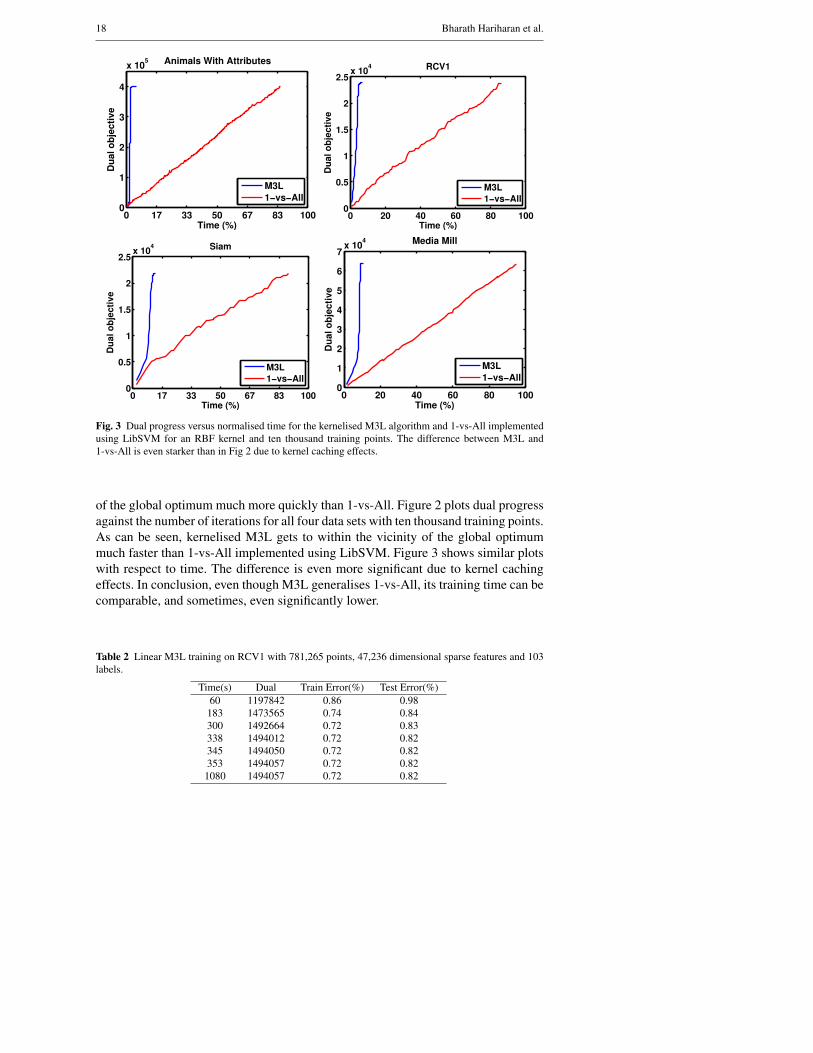
0 17 33 50 67 83 1000

1

2

3

4

x 105

Time (%)

Du

al

ob

jec

tiv

e

Animals With Attributes

M3L

1−vs−All

0 20 40 60 80 1000

0.5

1

1.5

2

2.5x 10

4

Du

al o

bje

cti

ve

Time (%)

RCV1

M3L

1−vs−All

0 17 33 50 67 83 1000

0.5

1

1.5

2

2.5x 10

4

Time (%)

Du

al o

bje

cti

ve

Siam

M3L

1−vs−All

0 20 40 60 80 1000

1

2

3

4

5

6

7x 10

4

Time (%)

Du

al

ob

jec

tiv

e

Media Mill

M3L

1−vs−All

Fig. 3 Dual progress versus normalised time for the kernelised M3L algorithm and 1-vs-All implemented

using LibSVM for an RBF kernel and ten thousand training points. The difference between M3L and

1-vs-All is even starker than in Fig 2 due to kernel caching effects.

of the global optimum much more quickly than 1-vs-All. Figure 2 plots dual progress

against the number of iterations for all four data sets with ten thousand training points.

As can be seen, kernelised M3L gets to within the vicinity of the global optimum

much faster than 1-vs-All implemented using LibSVM. Figure 3 shows similar plots

with respect to time. The difference is even more significant due to kernel caching

effects. In conclusion, even though M3L generalises 1-vs-All, its training time can be

comparable, and sometimes, even significantly lower.

Table 2 Linear M3L training on RCV1 with 781,265 points, 47,236 dimensional sparse features and 103

labels.

Time(s) Dual Train Error(%) Test Error(%)

60 1197842 0.86 0.98

183 1473565 0.74 0.84

300 1492664 0.72 0.83

338 1494012 0.72 0.82

345 1494050 0.72 0.82

353 1494057 0.72 0.82

1080 1494057 0.72 0.82


Finally, to demonstrate that our code scales to large problems, we train linear

M3L on RCV1 with 781,265 points, 47,236 dimensional sparse features and 103

labels. Table 2 charts dual progress and train and test error with time. As can be seen,

the model is nearly fully trained in under six minutes and converges in eighteen.

7.2 Incorporating Prior Knowledge for Zero-Shot Learning

In this Section, we investigate whether the proposed M3L formulation can improve

label prediction accuracy in a zero-shot learning scenario. Zero-shot learning has two

major components as mentioned earlier. The first component deals with generating

an intermediate level representation, generally based on attributes for each data point.

The second concerns itself with how to map test points in the intermediate representa-

tion to points representing novel categories. Our focus is on the former and the more

accurate prediction of multiple, intermediate attributes (labels) when their correlation

statistics on the training and test sets are significantly different.

7.2.1 Animals with Attributes

The Animals with Attributes data set (Lampert et al., 2009) has forty training animal

categories, such as Dalmatian, Skunk, Tiger, Giraffe, Dolphin, etc. and the following

ten disjoint test animal categories: Humpback Whale, Leopard, Chimpanzee, Hip-

popotamus, Raccoon, Persian Cat, Rat, Seal, Pig and Giant Panda. All categories

share a common set of 85 attributes such as has yellow, has spots, is hairless, is big,

has flippers, has buckteeth, etc. The attributes are densely correlated and form a fully

connected graph. Each image in the database contains a dominant animal and is la-

belled with its 85 attributes. There are 24,292 training images and 6,180 test images.

We use 252 dimensional PHOG features that are provided by the authors. M3L train-

ing times for this data set are reported in Table (1a).

We start by visualising the influence ofR. We randomly sample 200 points from

the training set and discard all but two of the attributes – “has black” and “is weak”.

These two attributes were selected as they are very weakly correlated on our training

set, with a correlation coefficient of 0.2, but have a strong negative correlation of -0.76

on the test animals (Leopards, Giant Pandas, HumpbackWhales and Chimpanzees all

Fig. 4 Sample training (top) and test (bottom) images from the Animals with Attributes data set.


−1 −0.5 0 0.5 115

20

25

30

35

40

Ha

mm

ing

Lo

ss (

%)

r

Fig. 5 Test Hamming loss versus classifier correlation.

have black but are not weak). Figure 5 plots the Hamming loss on the test set as we set

R = [1 r; r 1], plug it into the M3L formulation, and vary r from -1 to +1. Learning

independent classifiers for the two attributes (r = 0) can lead to a Hamming loss

of 25% because of the mismatch between training and test sets. This can be made

even worse by incorrectly choosing, or learning using structured output prediction

techniques, a prior that forces the two labels to be positively correlated. However,

if our priors are generally correct, then negatively correlating the classifiers lowers

prediction error.

We now evaluate performance quantitatively on the same training set but with

all 85 labels. We stress that in the zero shot learning scenario no training samples

from any of the test categories are provided. As is commonly assumed (Farhadi et al.,

2009, 2010; Lampert et al., 2009; Palatucci et al., 2009), we only have access to yc

which is the set of attributes for a given test category. Furthermore we require, as

additional information, the prior distribution over test categories p(c). For the M3L

formulation we set R =∑10

c=1p(c)ycy

tc. Under this setup, learning independent

classifiers using 1-vs-All yields a Hamming loss of 29.38%. The Hamming loss for

M3L, with the specific choice of R, is 26.35%. This decrease in error is very sig-

nificant given that 1-vs-All, trained on all 24,292 training points, only manages to

reduce error to 28.64%. Thus M3L, with extra knowledge, in the form of just test

category distributions, can dramatically reduce test error. The results also compare

favourably to other independent methods such as BoostTexter (Schapire & Singer,

2000) (30.28%), power set multi-class classification (32.70%), 5 nearest neighbours

(31.79%), regression (Hsu et al., 2009) (29.38%) and ranking (Crammer & Singer,

2003) (34.84%).

7.2.2 Benchmark Data Sets

We also present results on the fMRI-Words zero-shot learning data set of (Mitchell et al.,

2008). The data set has 60 categories out of which we use 48 for training and 12 for

testing. Each category is described by 25 real valued attributes which we convert to

binary labels by thresholding against the median attribute value. Prior information

about which attributes occur in which novel test categories is provided in terms of a


knowledge base. The experimental protocol is kept identical to the one used in An-

imals with Attributes. R is set to∑10

c=1p(c)ycy

tc where yc comes from the knowl-

edge base and p(c) is required as additional prior information. We use 400 points for

training and 648 points for testing. The test Hamming loss for M3L and various inde-

pendent methods is given in Table 3. The M3L results are much better than 1-vs-All

with the test Hamming loss being reduced by nearly 7%. This is noteworthy since

even if 1-vs-All were trained on the full training set of 2592 points, it would decrease

the Hamming loss by just over 5% to 48.79%.

Table 3 Test Hamming loss (%) on benchmark data sets.

Method fMRI-Words SIAM Media Mill RCV1 Yeast a-Yahoo

M3L 47.29 8.41 3.78 3.45 24.99 9.897

1-vs-All 53.97 11.15 4.69 4.25 26.93 11.35

BoostTexter 49.89 12.91 4.91 4.12 31.82 13.17

Power Set 48.69 14.01 6.27 3.71 32.32 17.81

Regression 53.76 11.19 4.69 4.26 26.70 11.36

Ranking 52.38 9.41 9.06 5.67 28.02 10.27

5-NN 50.81 12.51 4.74 4.47 28.82 13.04

Table 3 also presents results on some other data sets. Unfortunately, most of them

have not been designed for zero-shot learning. Siam (SIA), Media Mill (Snoek et al.,

2006), RCV1 (Lewis et al., 2004) and Yeast (Elisseeff & Weston, 2001) are tradi-

tional multi-label data sets with matching training and test set statistics. The a-PASCAL+a-

Yahoo (Farhadi et al., 2009) data set has different training and test categories but does

not include prior information about which attributes are relevant to which test cate-

gories. Thus, for all these data sets, we sample the original training set to create a

new training subset which has different label correlations than the provided test set.

The remainder of the original training points are used only to estimate the R matrix.

As Table 3 indicates, by incorporating prior knowledge M3L can do better than all

the other methods which assume independence.

8 Conclusions

We developed the M3L formulation for learning a max-margin multi-label classifier

with prior knowledge about densely correlated labels. We showed that the number

of constraints could be reduced from exponential to linear and, in the process, gener-

alised 1-vs-All multi-label classification. We also developed efficient optimisation al-

gorithms that were orders of magnitude faster than the standard cutting plane method.

Our kernelised algorithm was significantly faster than even the 1-vs-All technique

implemented using LibSVM and hence our code, available from (Hariharan et al.,

2010a), can also be used for efficient independent learning. Finally, we demonstrated

on multiple data sets that incorporating prior knowledge using M3L could improve

prediction accuracy over independent methods. In particular, in zero-shot learning

scenarios, M3L trained on 200 points could outperform 1-vs-All trained on nearly


25,000 points on the Animals with Attributes data set and the M3L test Hamming

loss on the fMRI-Words data set was nearly 7% lower than that of 1-vs-All.

Acknowledgements

We would like to thank Alekh Agarwal, Brendan Frey, Sunita Sarawagi, Alex Smola

and Lihi Zelnik-Manor for helpful discussions and feedback.

A Pseudo Code of the Kernelised M3L Algorithm

The dual that we are trying to solve is:

maxα

L∑

l=1

αtl(∆

−l−∆+

l)− 2

L∑

l=1

L∑

k=1

RlkαtlYlKYkαk (46)

s.t

0 ≤ α ≤ C1

where αl = [α1l, . . . αNl], Yl = diag([y1l . . . yNl]) and K = φ(X)tφ(X). Algorithm 1 describes

the training algorithm. The algorithm relies on picking two variables at each step and optimising over them

keeping all the others constant. If the two variables are αpl and αql (note that we choose two variables

corresponding to the same label l), then at each step we maximise h(δpl, δql) = D2(α+[δpl, δql,0t]t)−

D2(α) subject to −αpl ≤ δpl ≤ C − αpl and −αql ≤ δql ≤ C − αql Here, the indices have been

reordered so that αpl, αql occupy the first two indices. D2 is the dual objective function. It can be seen

that h(δpl, δql) comes out to be:

h(δpl, δql) =−2(δ2plKppRll + δ2qlKqqRll + 2δplδqlyplyqlKpqRll)

+δplgpl + δqlgql (47)

Here gpl = ∇plD2 and similarly gql = ∇qlD2. Since h is basically a quadratic function, it can be

written as:

h(δpq) = −1

2δpqQpqδpq + gt

pqδpq (48)

where

δpq=

[

δplδql

]

(49)

Qpq=

[

4KppRll 4KpqRllyplyql4KpqRllyplyql 4KqqRll

]

(50)

gpq=

[

gplgql

]

(51)

The constraints too can be written in vector form as:

mpq ≤ δpq ≤Mpq (52)

where

mpq =

[

−αpl

−αql

]

(53)

Mpq =

[

C − αpl

C − αql

]

(54)


Therefore at each step we solve a 2-variable quadratic program with box constraints. The algorithm to do

so is described later.

The variables αpl and αql being optimised over need to be chosen carefully. In particular we need to

ensure that the matrix Qpq is positive definite so that it can be maximised easily. We also need to make

sure that none of αpl and αql has projected gradient 0. The projected gradient of αpl, denoted here as gpl,is given by:

gpl =

gpl if αpl ∈ (0, C)min(0, gpl) if αpl = Cmax(0, gpl) if αpl = 0

(55)

We also use some heuristics when choosing p and q. It can be seen that the unconstrained maximum

of h is given by:

hmaxpq =

g2plKqq + g2

qlKpp − 2gplgqlyplyqlKpq

8Rll(KppKqq −K2pq)

(56)

This is an upper bound on the dual progress that we can achieve in an iteration and we pick p and q such

that hmaxpq is as big as possible.

Algorithm 1 Kernelised M3L

1: θik ← 0 ∀i, k2: gik ← ∆−

ik−∆+

ik3: repeat

4: for i = 1 to N do

5: ui ← 06: end for

7: l← argmaxk(maxi | gik |)8: for iteration = 1 to L do

9: p← argmaxi | gil |10: Sp ← {j : Kpj <

√

KppKjj and gjk 6= 0}11: if Sp 6= φ then

12: q ← argmaxj∈Sphmaxpj

13: (δpl, δql)←Solve2DQP(Qpq ,gpq ,mpq ,Mpq)

14: αpl ← αpl + δpl15: αql ← αql + δql16: for i = 1 to N do

17: gil ← gil − 4Rllyil(Kipyplδpl +Kiqyqlδql)18: ui ← ui + (Kipyplδpl +Kiqyqlδql)19: end for

20: else

21: δpl ←Solve1DQP(4KppRll, gpl,−αpl, C − αpl)

22: αpl ← αpl + δpl23: for i = 1 to N do

24: gil ← gil − 4RllyilKipyplδpl25: ui ← ui +Kipyplδpl26: end for

27: end if.

28: for k ∈ {1, . . . , L}\{l} do29: for i = 1 to N do

30: gik ← gik − 4Rklyikui

31: end for

32: end for

33: end for

34: until | gik |< τ ∀i, k


Algorithm 2 solves the problem:

maxm≤x≤M

−1

2xtQx+ gtx (57)

where x is 2-dimensional. Setting the gradient = 0, we get that the unconstrained maximum is at Q−1g.

If this point satisfies the box constraints, then we are done. If not, then we need to look at the boundaries

of the feasible set. This can be done by clamping one variable to the boundary and maximising along the

other, which becomes a 1-dimensional quadratic problem. Solve1DQP(a,b, m, M), referenced in lines 21

of Algorithm 1 and lines 6, 9, 12 and 13 solves a 1-dimensional QP with box constraints:

maxm≤x≤M

−1

2ax2 + bx (58)

The solution to this is merely min(M,max(m, ba)).

Algorithm 2 Solve2DQP(Q,g,m,M)

1: x∗ = Q−1g = 1

Q11Q22−Q2

12

[

Q22g1 −Q12g2Q11g2 −Q12g1

]

2: x0 = min(M,max(m,x∗));3: if x∗ ∈ [m,M] then4: return x∗

5: else if x∗1∈ [l1, u1] then

6: x1 ← Solve1DQP (Q11, g1 −Q12x02,m1,M1)

7: return (x1, x02)

8: else if x∗2∈ [l2, u2] then

9: x2 ← Solve1DQP (Q22, g2 −Q12x01,m2,M2)

10: return (x01, x2)

11: else

12: x1 ← [x01, Solve1DQP (Q22, g2 −Q12x0

1,m2,M2)]

13: x2 ← [Solve1DQP (Q11, g1 −Q12x02,m1,M1), x0

2]

14: d1 ← −1

2x1tQx1 + gtx1

15: d2 ← −1

2x2tQx2 + gtx2

16: if d1 > d2 then

17: return x1

18: else

19: return x2

20: end if

21: end if

B Proof of Convergence of the Kernelised M3L Algorithm

We now give a proof of convergence of the kernelised M3L algorithm. The proof closely follows the one

in Keerthi & Gilbert (2002) and is provided for the sake of completeness.

B.1 Notation

We denote vectors in bold small letters, for example v. If v is a vector of dimension d, then vk, k ∈{1, . . . , d} is the k-th component of v, and vI , I ⊆ {1, . . . , d} denotes the vector with components

vk, k ∈ I (with the vk’s arranged in the same order as in v). Similarly, matrices will be written in bold


capital letters, for example A. If A is an m × n matrix, then Aij represents the ij-th entry of A, and

AIJ represents the matrix with entries Aij , i ∈ I, j ∈ J .

A sequence is denoted as {an}, and an is the n-th element of this sequence. If a is a limit point of

the sequence, we write an → a.

B.2 The Optimisation Problem

The dual that we are trying to solve is:

maxα

L∑

l=1

αtl ( ∆−

l−∆+

l)

− 2L∑

l=1

L∑

k=1

RlkαtlYlKYkαk (59)

s.t

0 ≤ α ≤ C1

whereαl = [α1l, . . . αNl],Yl = diag([y1l . . . yNl]),K = φ(X)tφ(X) and∆±l

= (∆l(y1,±y1l), . . . , ∆l(yN ,±yNl)).This can be written as the following optimisation problem:

Problem:

maxα

f(α) = −1

2α

tQα+ ptα (60)

s.t

l ≤ α ≤ u

Here the vectorα = [α11 . . . α1L, α21, . . . αNL]t andQ = 4YK⊗RY where⊗ is the Kronecker

product. Y = diag([y11 . . . y1L, y21, . . . yNL]). p = ∆−l−∆+

l, l = 0 and u = C1. We assume

that R and K are both positive definite matrices. The eigenvalues of K ⊗ R are then λiµj (see, for

example, Bernstein (2005)), where λi are the eigenvalues ofK and µj are the eigenvalues ofR. Because

all eigenvalues of both R and K are positive, so are the eigenvalues of K ⊗ R and thus Q is positive

definite. Thus the dual we are trying to solve is a strictly convex quadratic program.

Our algorithm will produce a sequence of vectors {αn} where {αi} is the vector before the i-thiteration. For brevity, we denote the gradient ∇f(αn) as gn and the projected gradient ∇P f(αn) asgn. The algorithm stops when all the projected gradients have magnitude less than τ . It can be easily seenthat by reducing τ , we can get arbitrarily close to the optimum.

Hence, in the following, we only need to prove that the algorithm will terminate in a finite number of

steps.

B.3 Convergence

In this section we prove that the sequence of vectors αn converges.

Note the following:

– In each iteration of the algorithm, we optimise over a set of variables, which may either be a single

variable αpl or a pair of variables {αpl, αql}.

– The projected gradient of all the chosen variables is non zero at the start of the iteration.

– At least one of the chosen variables has projected gradient with magnitude greater than τ .


Consider the n-th iteration. Denote by B the set of indices of the variables chosen: B = {(p, l)}or B = {(p, l), (q, l)}. Without loss of generality, reorder variables so that the variables in B occupy

the first |B| indices. In the n-th iteration, we optimise f over the variables in B keeping the rest of the

variables constant. Thus we have to maximise h(δB) = f(αn + [δtB , 0t]t)− f(αn). This amounts to

solving the optimisation problem:

maxδB

h(δB) = −1

2δtBQBBδB − δ

tB(Qα

n)B

+ptBδB (61)

s.t

lB −αB ≤ δB ≤ uB −αB

Note that since gnB = −(Qαn)B + pB

h(δB) = −1

2δtBQBBδB + δ

tBgn

B (62)

QBB is positive definite since Q is positive definite, so this QP is convex. Hence standard theorems(see

Nocedal & Wright (2006)) tell us that δ∗B optimises (61) iff it is feasible and

∇P h(δ∗B) = 0 (63)

Then we have that αn+1 = αn + δ∗, where δ∗ = [δ∗tB , 0t]t. Now

∇h(δ∗B) = −QBBδ∗B + gn

B (64)

Also,

gn+1

B= −(Qα

n+1)B + pB (65)

= −(Q(αn + [δ∗tB , 0t]t))B + pB

= (−(Qαn)B + pB)−QBBδ

∗B

= gnB −QBBδ

∗B

= ∇h(δ∗B)

Then (65) means that:

gn+1

B= ∇P h(δ∗B) (66)

Using (63)

gn+1

B= ∇P h(δ∗B) = 0 (67)

This leads us to the following lemma:

Lemma 1 Let αn be the solution at the start of the n-th iteration. Let B be the set of indices of the

variables over which we optimise. Let the updated solution be αn+1. Then

1. gn+1

B= 0

2. αn+1 6= αn

3. If ljk < αn+1

jk< ujk then gn+1

jk= 0 ∀(j, k) ∈ B

Proof 1. This follows directly from (67).

2. If αn+1 = αn, then δ∗B = 0 and so, from (65), gn+1

B= ∇h(0) = gn

B . This means that from

(67) gnB = gn+1

B= 0. But this is a contradiction since we required that all variables in the chosen

set have non zero projected gradient before the start of the iteration.

3. Since the final projected gradients are 0 for all variables in the chosen set (from (67)), if ljk <

αn+1

jk< ujk then gn+1

jk= 0 ∀(j, k) ∈ B


Lemma 2 In the same setup as the previous lemma, f(αn+1)− f(αn) ≥ σ‖αn+1 −αn‖2, for somefixed σ > 0.

Proof

f(αn+1)− f(αn) = h(δ∗B)

= −1

2δ∗tBQBBδ

∗B + δ

∗tB gn

B (68)

where δ∗B is the optimum solution of Problem (61). Now, note that since δ∗B is feasible and 0 is feasible

and h is concave, we have that(see Nocedal & Wright (2006)):

(0− δ∗B)t∇h(δ∗B) ≤ 0 (69)

⇒ δ∗tBQBBδ

∗B − δ

∗tB gn

B ≤ 0 (70)

⇒ δ∗tBQBBδ

∗B ≤ δ

∗tB gn

B (71)

This gives us that

−1

2δ∗tBQBBδ

∗B + gnt

B δ∗B ≥

1

2δ∗tBQBBδ

∗B (72)

⇒ f(αn+1)− f(αn) ≥1

2δ∗tBQBBδ

∗B (73)

⇒ f(αn+1)− f(αn) ≥ νB1

2δ∗tB δ

∗B (74)

where νB is the minimum eigenvalue of the matrix QBB . Since QBB is positive definite always, this

value is always greater than zero, and bounded below by the minimum eigenvalue among all 2×2 positive

definite sub matrices ofQ. Thus

f(αn+1)− f(αn) ≥ σδ∗tB δ∗B

= σ‖αn+1 −αn‖2 (75)

for some fixed σ ≥ 0.

Theorem 1 The sequence {αn} generated by our algorithm converges.

Proof From Lemma 2, we have that f(αn+1)− f(αn) ≥ 0. Thus the sequence {f(αn)} is monoton-

ically increasing. Since it is bounded from above (by the optimum value) it must converge. Since conver-

gent sequences are Cauchy, this sequence is also Cauchy. Thus for every ǫ, ∃n0 s.t f(αn+1)− f(αn) ≤σǫ2 ∀n ≥ n0. Again using Lemma 2, we get that

‖αn+1 −αn‖2 ≤ ǫ2 (76)

for every n ≥ n0. Hence the sequence {αn} is Cauchy. The feasible set of α is closed and compact, so

Cauchy sequences are also convergent. Hence {αn} converges.


B.4 Finite termination

We have shown that {αn} converges. Let α be a limit point of {αn}. We will start from the assumption

that the algorithm runs for an infinite number of iterations and then prove a contradiction.

Call the variable αik as τ -violating if the magnitude of the projected gradient gik is greater than

τ . Note that at every iteration, the chosen set of variables contains at least one that is τ -violating. Nowsuppose the algorithm runs for an infinite number of iterations. Then it means that the sequence of iterates

αk contains an infinite number of τ -violating variables. Since there are only a finite number of distinct

variables, we have that at least one variable figures as a τ -violating variable in the chosen setB an infinite

number of times. Suppose that αil is one such variable, and let {kil} be the sub-sequence in which this

variable is chosen as a τ -violating variable.

Lemma 3 For every ǫ ∃k0ils.t | α

kil+1

il− α

kil

il|≤ ǫ ∀kil > k0

il.

Proof We have that sinceαk → α,αkil → α, andαkil+1 → α. Thus, for any given ǫ ∃ k0ilsuch that

| αkil

il− αil |≤ ǫ/2 ∀kil > k0il (77)

| αkil+1

il− αil |≤ ǫ/2 ∀kil + 1 > k0il (78)

This gives, by triangle inequality,

| αkil+1

il− α

kil

il|≤ ǫ ∀kil > k0il (79)

Lemma 4 | gil |≥ τ , where gil is the derivative of f w.r.t αil at α.

Proof This is simply because of the fact that | gkil

il|≥ τ for every kil, and the absolute value of the

derivative w.r.t αil is a continuous function of α, and αkil → α.

We use some notation. If αkil

il∈ (lil, uil) and if α

kil+1

il= lil or α

kil+1

il= uil, then we say that

“kil is int→ bd”, where “int” stands for interior and “bd” stands for boundary. Similar interpretations are

assumed for “bd→ bd” and “int→ int”. Thus each iteration kil can be of one of only four possible kinds:int→ int,int→ bd, bd→ int and bd→ bd. We will prove that each of these kinds of iterations can only

occur a finite number of times.

Lemma 5 There can be only a finite number of int→ int and bd→ int transitions.

Proof Suppose not. Then we can construct an infinite sub-sequence {sil} of the sequence {kil} that

consists of these transitions. Then we have that gsil+1

il= 0, using Lemma 1. Hence g

sil+1

il→ 0. Since

the gradient is a continuous function of α, and since αsil+1 → α, we have that gsil+1

il→ gil. But this

means gil = 0, which contradicts Lemma 4.

Lemma 6 There can be only a finite number of int→ bd transitions.

Proof Suppose that we have completed sufficient number of iterations so that all int→ int and bd→ int

transitions have completed. The next int→ bd transition will place αil on the boundary. Since there are

no bd→ int transitions anymore, αil will stay on the boundary henceforth. Hence there can be no more

int→ bd transitions.

Lemma 7 There can only be a finite number of bd→ bd transitions.

Proof Suppose not, i.e there are an infinite number of bd→ bd transitions. Let til be the sub-sequenceof kil consisting of bd→ bd transitions. Now, the sequence α

tilil→ αil and is therefore Cauchy. Hence

∃n1 s.t

| αtilil− α

til+1

il|≤ ǫ≪ uil − lil ∀til ≥ n1 (80)


Similarly, because the gradient is a continuous function of α, the sequence {gtilil} is convergent and

therefore Cauchy. Hence ∃n2 s.t

| gtilil− g

til+1

il|≤

τ

2∀kil ≥ n2 (81)

Also, from the previous lemmas, ∃n3 s.t til is not int→ int, bd→ int or int→ bd ∀til ≥ n3.

Take n0 = max(n1, n2, n3). Now, consider til ≥ n0. Without loss of generality, assume that

αtilil

= lil. Then, since | gtilil|≥ τ , we must have that g

tilil≥ τ . From (80), and using the fact that this is

a bd→ bd transition, we must have that

αtil+1

il= lil (82)

From (81), we have that

gtil+1

il≥

τ

2(83)

From (82) and (83), we have that gtil+1

il≥ τ

2, which contradicts Lemma 1.

But if all int → int, int → bd, bd → int and bd → bd transitions are finite, then αil cannot be

τ -violating an infinite number of times and hence we have a contradiction. This gives us the following

theorem:

Theorem 2 Our algorithm terminates in finite number of steps.

References

The SIAM Text Mining Competition 2007 http://www.cs.utk.edu/tmw07/).

Bernstein, Dennis S. Matrix Mathematics. Princeton University Press, 2005.

Boutell, M., Luo, J., Shen, X., and Brown, C. Learning multi-label scene classification. Pattern Recogni-

tion, 37(9):1757–1771, 2004.

Cai, L. and Hofmann, T. Exploiting known taxonomies in learning overlapping concepts. In Proceedings

of the International Joint Conference on Artificial Intelligence, pp. 714–719, 2007.

Cesa-Bianchi, N., Gentile, C., and Zaniboni, L. Incremental algorithms for hierarchical classification.

Journal of Machine Learning Research, 7:31–54, 2006.

Chang, C.-C. and Lin, C.-J. LIBSVM: a library for support vector machines, 2001. Software available at

http://www.csie.ntu.edu.tw/˜cjlin/libsvm.

Cheng, W., Dembczynski, K., and Huellermeier, E. Graded multilabel classification: The ordinal case. In

Proceedings of the International Conference on Machine Learning, 2010.

Crammer, K. and Singer, Y. A family of additive online algorithms for category ranking. Journal of

Machine Learning Research, 3:1025–1058, 2003.

Dekel, O. and Shamir, O. Multiclass-multilabel classification with more classes than examples. In Pro-

ceedings of the International Conference on Artificial Intelligence and Statistics, 2010.

Elisseeff, A. and Weston, J. A kernel method for multi-labelled classification. In Advances in Neural

Information Processing Systems, pp. 681–687, 2001.

Evgeniou, T., Micchelli, C. A., and Pontil, M. Learning multiple tasks with kernel methods. Journal of

Machine Learning Research, 2005.

Fan, R. E., Chen, P. H., and Lin, C. J. Working set selection using second order information for training

SVM. Journal of Machine Learning Research, 6:1889–1918, 2005.

Fan, R.-E., Chang, K.-W., Hsieh, C.-J., Wang, X.-R., and Lin, C.-J. Liblinear: A library for large linear

classification. Journal of Machine Learning Research, 9:1871–1874, 2008.

Farhadi, A., Endres, I., Hoeim, D., and Forsyth, D. A. Describing objects by their attributes. In Proceedings

of the IEEE Conference on Computer Vision and Pattern Recognition, 2009.

Farhadi, A., Endres, I., and Hoeim, D. Attribute-centric recognition for cross-category generalization. In

Proceedings of the IEEE Conference on Computer Vision and Pattern Recognition, 2010.

Hariharan, B., Vishwanathan, S. V. N., and Varma, M., 2010a. M3L code

http://research.microsoft.com/˜manik/code/M3L/download.html.

http://www.csie.ntu.edu.tw/~cjlin/libsvm


Hariharan, B., Zelnik-Manor, L., Vishwanathan, S. V. N., and Varma, M. Large scale max-margin multi-

label classification with priors. In Proceedings of the International Conference on Machine Learning,

2010b.

Hsieh, C.-J., Chang, K.-W., Lin, C.-J., Keerthi, S. S., and Sundarajan, S. A dual coordinate descent method

for large-scale linear svm. In Proceedings of the International Conference on Machine Learning, 2008.

Hsu, D., Kakade, S., Langford, J., and Zhang, T. Multi-label prediction via compressed sensing. In

Advances in Neural Information Processing Systems, 2009.

Ji, S., Sun, L., Jin, R., and Ye, J. Multi-label multiple kernel learning. In Advances in Neural Information

Processing Systems, pp. 777–784, 2008.

Keerthi, S. S. and Gilbert, E. G. Convergence of a generalized SMO algorithm for SVM classifier design.

Machine Learning, 46(1–3):351–360, 2002.

Lampert, C. H., Nickisch, H., and Harmeling, S. Learning to detect unseen object classes by between-class

attribute transfer. In Proceedings of the IEEE Conference on Computer Vision and Pattern Recognition,

2009.

Lewis, D., Yang, Y., Rose, T., and Li, F. RCV1: A new benchmark collection for text categorization

research. Journal of Machine Learning Research, 5:361–397, 2004.

Li, X., Wang, L., and Sung, E. Multi-label SVM active learning for image classification. In Proceedings

of the IEEE International Conference on Image Processing, pp. 2207–2210, 2004.

Lin, C. J., Lucidi, S., Palagi, L., Risi, A., and Sciandrone, M. Decomposition algorithm model for singly

linearly-constrained problems subject to lower and upper bounds. Journal of Optimization Theory and

Applications, 141(1):107–126, April 2009.

McCallum, A. Multi-label text classification with a mixture model trained by EM. In AAAI 99 Workshop

on Text Learning, 1999.

Mitchell, T., Shinkareva, S., Carlson, A., Chang, K.-M., Malave, V., Mason, R., and Just, A. Predicting

human brain activity associated with the meanings of nouns. Science, 320:1191–1195, 2008.

Nocedal, J. and Wright, S. J. Numerical Optimization. Springer, 2nd edition, 2006.

Palatucci, M., Pomerleau, D., Hinton, G., and Mitchell, T. Zero-shot learning with semantic output codes.

In Advances in Neural Information Processing Systems, 2009.

Platt, J. Fast training of support vector machines using sequential minimal optimization. In Advances in

Kernel Methods – Support Vector Learning, pp. 185–208, 1999.

Rifkin, R. and Khautau, A. In defense of one-vs-all classification. Journal of Machine Learning Research,

5:101–141, 2004.

Rousu, J., Saunders, C., Szedmak, S., and Shawe-Taylor, J. Kernel-based learning of hierarchical multil-

abel classification models. Journal of Machine Learning Research, 7:1601–1626, 2006.

Schapire, R. E. and Singer, Y. Boostexter: A boosting-based system for text categorization. Machine

Learning, 39(2/3):135–168, 2000.

Snoek, C., Worring, M., van Gemert, J., Geusebroek, J.-M., and Smeulders, A. The challenge problem for

automated detection of 101 semantic concepts in multimedia. In Proceedings of ACM Multimedia, pp.

421–430, 2006.

Taskar, B., Guestrin, C., and Koller, D. Max-margin markov networks. In Advances in Neural Information

Processing Systems, 2003.

Tsochantaridis, I., Joachims, T., Hofmann, T., and Altun, Y. Large margin methods for structured and

interdependent output variables. Journal of Machine Learning Research, 6:1453–1484, 2005.

Tsoumakas, G. and Katakis, I. Multi-label classification: An overview. Int. Journal of Data Warehousing

and Mining, 3(3):1–13, 2007.

Ueda, N. and Saito, K. Parametric mixture models for multi-labeled text. Advances in neural information

processing systems, 2003.

Vishwanathan, S.V.N., sun, Zhaonan, Ampornpunt, Nawanol, and Varma, Manik. Multiple kernel learning

and the smo algorithm. In Advances in Neural Information Processing Systems 23. 2010.

Wang, G., Forsyth, D. A., and Hoeim, D. Comparative object similarity for improved recognition with few

or no examples. In Proceedings of the IEEE Conference on Computer Vision and Pattern Recognition,

2010.

Zhang, M.-L. and Wang, Z.-J. Mimlrbf: Rbf neural networks for multi-instance multi-label learning.

Neural Computing, 72(16–18):3951–3956, 2009a.

Zhang, M.-L. and Wang, Z.-J. Feature selection for multi-label naive bayes classification. Information

Sciences, 179(19):3218–3229, 2009b.

efficient max-margin multi-label classification with applications to

Documents