Efficient Edgebreaker for surfaces of arbitrary topology

THOMAS LEWINER1,2, HELIO LOPES1, JAREK ROSSIGNAC3, AND ANTONIO WILSON V IEIRA1,4

1PUC-RIO – Laboratorio Matmıdia – Rio de Janeiro – Brazil2INRIA – Geometrica Project – Sophia Antipolis – France

3GATECH – GVU Center – Atlanta – USA4UNIMONTES – CCET – Montes Claros – Brazil

tomlew@mat.puc-rio.br, lopes@mat.puc-rio.br, jarek@cc.gatech.edu, awilson@mat.puc-rio.br

Abstract. The typical surfaces models handled by contemporary Computer Graphics applications have millionsof triangles and numerous connected component, handles and bounding loops. Edgebreaker and Spirale Reversiare examples of efficient schemes to compress and decompress their connectivity. A surprisingly simple linear-time implementation has been proposed for triangulated surfaces homeomorphic to a sphere and was subsequentlyextended to surfaces with handles. Here, we further extend its scope to surfaces with multiple components, handles,and multiple bounding loops. The result is a simple and efficient compression/decompression solution for the broadclass of orientable manifold surfaces.

1 Introduction

The Edgebreaker scheme [9] encodes the connectivity ofany manifold triangle mesh homeomorphic to a sphere witha guaranteed worst case code of 1.83 bits per triangle [4].The Spirale Reversi algorithm [7] enhanced the Edgebreakerdecompression complexity fromO(n2) to O(n). But thetrue value of Edgebreaker and Spirale Reversi lies in the ef-ficiency and in the simplicity of their implementations [10],which is very concise. They can be simply implementedon a reduced topological data structure (the Corner–Table)which only uses two arrays of integers to represent the con-nectivity of the mesh. This simple algorithm has been ex-tended to deal with surfaces with handles in [13]. Becauseof its simplicity, Edgebreaker is viewed as the emergingstandard for 3D compression [17] and may provide an al-ternative for the current MPEG-4 standard which is basedon the Topological Surgery approach [14].

Prior Works. There are many different compression schemesfor triangular meshes. In order to encode efficiently theirgeometry, the best known methods traverse the cells of themesh, and differ in the way they encode this traversal. TheEdgebreaker scheme has been enhanced and adapted fromthe Topological Surgery [14] to yield an efficient but ini-tially restricted algorithm [9], and subsequently extendedto more general meshes [7, 15]. Edgebreaker encodes theconnectivity of the mesh by producing theclers string ofsymbols taken from the set C,L,E,R,S. A different approachencodes the connectivity of the mesh by the valence of itsvertices [6, 3]. Valence-based compression approaches arevery efficient, especially for regular meshes and it can alsobe extended to general polygonal meshes. Another approach[12] computes a uniquely defined traversal for a given mesh,

leading to asymptotically optimal results for the worst case.However, it is restricted to meshes without boundary andwithout handle.

The Spirale Reversi algorithm [7] enhanced the Edge-breaker original decompression [9] and the Wrap&Zip de-compression [11]. It reconstructs the connectivity encodedin the clers string in only one pass. However, it needs toread it in a reverse way.

The Edgebreaker algorithm has been previously ex-tended to efficiently support surfaces with handles in [13]:it introduces thehandlestream which stores in an efficientway two edges for each handle on the surface. Those edgestogether with theclers string are sufficient to recover allthe surface connectivity. This extension doesn’t add a newsymbol to the Edgebreaker originalclersset.

Surfaces with boundary are usually encoded by clos-ing each boundary curve, using a dummy vertex to maintainthe triangular structure [8, 9]. This is a very simple but ex-pensive solution: first, it requires encoding each boundaryedge a useless triangle; second, it requires extra code to lo-calize the dummy vertex; and third, it gives bad geometricalpredictors on the boundary. The original Edgebreaker en-codes boundary curves with an extra symbolM , and writingthe length of each boundary curve. This allows a better ge-ometrical prediction, but gives a complex implementationwith an implicit representation of the topology, and it re-quires extra codes which harm the coding of theclersstring.The scheme introduced here does not require more symbolthan the original Edgebreaker for closed surfaces, and en-code each boundary curve with only two integers.

Contributions. In this paper, we provide efficient and ro-bust extensions of the Edgebreaker compression and of the

associated Spirale Reversi decompression schemes for sur-faces with an arbitrary topology. This new approach isbased on a new semantics, which enables us to use theEdgebreakerclers string to encode the connectivity of asurface, possibly having any number of connected compo-nents, handles or boundary curves. To do so, we exploit atopological analogy between handles and boundaries, andcapitalize on the simplicity with which edges may be iden-tified in thetopologystream. Moreover, the resulting com-pression format represent separately the topology, the localconnectivity and the geometry of the surface, leading to asimple and robust implementation.

Paper outline. Section2 introduces some basic concepts.Section3 describes the Corner–Table data structure. Sec-tion4establishes some notation and presents important prop-erties that connect the surface duality to the Edgebreakeralgorithm. Section5 presents the algorithm overview. Sec-tions 6 and7 introduce, respectively, the enhanced Edge-breaker compression and the extended Spirale Reversi de-compression algorithms. The theoretical analysis of the al-gorithm is presented in Section8. Finally, Section9 showssome results and comparison with former Edgebreaker al-gorithm.

2 Basic concepts

We will consider an orientable triangulated combinatorialsurface. This is the general case of manifold triangle meshesembedded inR3, but we are only concerned with their con-nectivity, e.g., the triangle/vertex incident and the triangle/triangleadjacency information.

Definition 1 (Combinatorial surface) A triangle meshSis a combinatorial surface if:

– Every edge inS is bounding either one or two trian-gles.

– The link of a vertex inS is homeomorphic either to aninterval or to a circle.

The set of edges inS incident to only one triangleis called theboundaryof S, denoted by∂(S). A bound-ary curveof a surface is a maximal connected set of adja-cent edges of the boundary. Each boundary curve is closed.From now on, we denote byT (S), E(S) andV(S) the setof triangles, edges and vertices ofS.

Theorem 1 (Surface classification)[1] Any compact ori-ented connected surfaceS is homeomorphic to a sphere(g(S) = 0) or a connected sum ofg(S) tori (g(S) > 0),in both cases with possibly some finite numberb(S) ≥ 0 ofopen disks removed. The numberg(S) is called thegenus

of S, and b(S) its number of boundary curves. The Eu-ler characteristicχ(S) of S is equal toχ(S) = |T (S)| −|E(S)|+ |V(S)| = 2− 2 · g(S)− b(S).

Figure 1:Handlebody decomposition of a torus [13].

Each torus of the connected sum above is composed bytwo 1–handles, as shown on Figure1. This decompositioncan be generalized using the Handlebody theory [13]. Sincethis concept of handle contains a complete representation ofboundaries, it will play a fundamental role in our algorithm.

3 Corner–Table Data Structure

The Corner–Table is a very concise data structure for trian-gular meshes. It uses the concept ofcorner to represent theassociation of a triangle with one of its bounding vertices,or equivalently the association a triangle with its boundingedge opposite to that corner: it may be viewed as a com-pact version of the half–edge representation of triangularmeshes.

Figure 2:Corner notations.

In this data structure, the corners, the vertices and thetriangles are indexed by non-negative integers. Each trian-gle is represented by 3 consecutive corners that define itsorientation. For example, corners 0, 1 and 2 correspondto the first triangle; the corners 3, 4 and 5 correspond tothe second triangle and so on. . . As a consequence, a cor-ner with indexc is associated with the triangle of indexc.t = c ÷ 3. Assuming a counter-clockwise orientation,

for each cornerc of a trianglec.t, the next (c.n) and previ-ous (c.p) corners ofc.t are obtained by the use of the fol-lowing expressions:c.n = 3 · c.t + (c + 1) mod 3, andc.p = 3 · c.t + (c + 2) mod 3.

The Corner–Table data structure represents the geome-try of a surfaceS by the association of each cornerc with itsgeometrical vertex indexc.v. The edge-adjacency betweenthe neighboring triangles ofS is represented by associatingwith each cornerc its opposite cornerc.o, which has thesame opposite geometrical edge (formallyc.n.v = c.o.p.vandc.o.o = c, see Figure2). This information is stored intwo integer arrays, called the V and O tables. For conve-nience, we define the left corner ofc asc.l = c.p.o and theright corner ofc asc.r = c.n.o.

Corner O table V table

0 3 01 10 12 7 2

3 0 34 6 25 11 1

6 4 07 2 38 9 1

9 8 210 1 311 5 0

Figure 3: A tetrahedron with its corners and its Corner–Table.

To illustrate the data structure tables consider the tetra-hedron of Figure3.

4 Surface Duality and the Edgebreaker

In this section we provide some notations and introduce im-portant properties that will be used to describe and analyzethe algorithm.

The primal graphof a surfaceS is the simple graphwhose nodes are the verticesV(S) of S and whose lines arethe edgesE(S) of S (e.g., a line connect adjacent vertices).The dual graphof a surfaceS is the graph whose nodesare the trianglesT (S) of S and whose lines represent theedgesE(S) of S (e.g., a line connect adjacent triangles).For example, Figure4(a)and4(b)represents the primal andthe dual graph of a triangulated sphere.

Edgebreaker algorithms encode the dual and primalgraphs of a triangular meshS by an efficient use of sur-face duality. They extract a spanning treeΘ(S) of the dualgraph ofS (see Figure5(a)) by traversing and encoding the

Figure 4:(left): the primal graph and (right): the dual graphof a triangulated sphere.

Figure 5: (left): a dual spanning treeΘ(S) extracted fromthe dual graph of Figure4(b). (right): the primal remainderΓ(S) of Θ(S), which is a subgraph of the primal graph ofFigure4(a).

triangles ofS in a spiral way. This encoding describes si-multaneously the primal remainder (see Figure5(b)): Theprimal remainderis the maximal subgraph of the primalgraph ofS which does not intersectΘ(S), in other words:

Definition 2 (primal remainder) Given a connected sur-faceS and a spanning treeΘ(S) of the dual graph ofS,theprimal remainderΓ(S) is the simple graph whose nodesare the verticesV(S) of S and whose lines are the edges ofS which are not inΘ(S).

The following theorem relates the Euler characteristicof the surface to the connectivity of the primal remainder.

Theorem 2 For any connected surfaceS and any dual span-ning treeΘ(S), the primal remainderΓ(S) is a connectedgraph with|V(S)| nodes and|V(S)| − χ(S) + 1 lines. Inparticular, Γ(S) is a tree if and only ifS is homeomorphicto a sphere.

Proof. ClearlyΓ(S) is connected, although the formal proofcan involve basic topological techniques as thickening [1]or cell collapse (the fundamental group is unchanged by re-moving a dual spanning tree [2]). By definition, Θ(S) isa tree with|T (S)| nodes, hence, it has|T (S)| − 1 lines.Also by definition,Γ(S) has|V(S)| nodes, and the num-ber of lines ofΘ(S) andΓ(S) together isE(S)| . Hence,

the number of lines ofΓ(S) is |E(S)| − (|T (S)| − 1) =|V(S)| − χ(S) + 1.Then, Γ(S) is a tree if and only if its number of nodesequals its number of lines plus one:|V(S)|−(|V(S)| − χ(S) + 1) =1. That is, iff the Euler characteristic ofS is 2, e.g., iffS isa sphere (see Theorem1). ¥

Figure 6: (left): a primal remainder on a torus (genus 1):the topmost and bottommost horizontal edges are identified,and also the leftmost and rightmost ones. (right) a primalremainder on an annulus (two boundary curves).

For example, in the case of a sphere, the primal re-mainder is a tree (see Figure5(b)). For a mesh with genusone or two boundaries, the primal remainder is a graph withtwo cycles (see Figures6(a) and 6(b)). And as a conse-quence of this fact, we can state the following theorem:

Theorem 3 For every spanning treeΨ(S) extracted fromΓ(S), the number of edges that are inΓ(S) but not inΨ(S)will be 2 · g(S) + b(S).

Proof. We know thatΓ(S) has|V(S)| nodes. Ψ(S) is aspanning tree ofΓ(S), then it also has|V(S)| nodes and|V(S)| − 1 lines. As a consequence, the number of lines ofΓ(S) that are not inΨ(S) is (|V(S)|−χ(S)+1)−(|V(S)|−1) = 2− χ(S) = 2 · g(S) + b(S). ¥

5 Algorithm overview

Original Edgebreaker The Edgebreaker algorithm tra-verses spirally the dual graph of a surface in order to gen-erate a spanning tree. At each step, a decision is made tomove from a triangleY to an adjacent triangleX. To per-form this decision, all visited triangles and their incidentvertices are marked. Let Left and Right denote the othertwo triangles that are incident upon X. Letv be the vertexcommon toX, Left, and Right. The edge opposed tov iscalled thegate. Five situations are distinguished accordingto Figure7. Those cases are denoted by the lettersC, L ,E, R andS. The arrow indicates the direction to the nexttriangle. Previously visited triangles are filled in gray.

v Left RightC not visited not visited not visitedL visited visited not visitedR visited not visited visitedE visited visited visitedS visited not visited not visited

Figure 7:The Edgebreaker encoding.

To have a concise implementation of the Edgebreaker,the compression is done by the use of a recursive procedurethat traverses the surface. The recursion starts only at trian-gles that are of typeS and compresses the branch adjacentto the right edge of such a triangle. When the correspond-ing E triangle is reached, the branch traversal is completeand the routine returns from the recursion to pursue the leftbranch.

The original Edgebreaker does not handle surfaces withgenus, and gives two options to compress the boundarycurves. The first one [4] consists in closing each bound-ary curve by adding a dummy vertex, and joining it to theboundary vertices to form dummy triangles. The mesh doesnot have any boundary anymore, and can be compressed us-ing the algorithm described above. This is a very simple butexpensive solution: first, it requires to encode each bound-ary edge a useless triangle; second, it requires extra codeto localize the dummy vertex; and third, it gives bad geo-metrical predictors on the boundary. The second option [9]encodes the first triangle which reaches the boundary withan extra symbolM and sends the length of the boundarycurve. At this step of the compression, encoding and re-moving thisM triangle joins the boundary curve reachedwith the external boundary curve, and the resulting meshhas one less boundary curve.

Handles When the surfaceS has genusg(S) > 0, theprimal remainderΓ(S) is not a tree anymore (see Theo-rem2). For a surface without boundary,Γ(S) has|V(S)| −χ(S) + 1 = |V(S)| − 1 + 2 · g(S) lines: there are2 · g(S)lines in excess [13]. These edges have been simply de-tected and efficiently encoded in [13], preserving the orig-inal Edgebreaker compression scheme. When the Edge-breaker traversing procedure finds anS triangle, the recur-sion starts and two situations are now distinguished. If the

(a) Reaching firstS triangle (b) Reaching secondS triangle

(c) The lower–right E trianglecloses the handle: the second Ssymbol is ahandleS.

(d) The upper–left E trianglecloses the handle: the first S sym-bol is ahandleS.

Figure 8:Coding of a torus: the creation ofhandleS trian-gles.

Left triangle has not been visited during the right branchtraversal (case of normalS), we move to the left neighborand continue our encoding of the left branch. Otherwise(case of a handleS) the pair of opposite corners separatedby the left edge of theS triangle are sent to a stream or afile calledtopologyand the routine returns. These cornerswill be matched during decompression to reconstruct thehandle. The encounter of anE that does not match anSagain terminates the compression process of the connectedcomponent.

Boundaries The work presented here extends these priorresults to surfaces with handles, multiple boundary curvesand multiple components. The former techniques for en-coding boundaries and holes introduced in [9] are morecostly, since they are using extra symbols or encoding moreelements. In particular, they do not guarantee anymore theworst case 1.83 bit per symbol. To improve the concise-ness of our codification, we distinguish two distinct cases:a connected component with one boundary curve, and withmore than one boundary curve.

Consider first a surface componentS with genusg(S)and only one boundary curve. We will close this compo-nent by adding a face incident to each boundary edge ofS,calledinfinite face. The resulted surfaceS+ has no bound-ary, and the same genus, i.e.,g(S+) = g(S). We couldalmost use the extended Edgebreaker algorithm of [13] toencodeS+. However, the infinity face is not a triangle.

(a) The first triangle is chosen ad-jacent to a boundary. The verticesof the central infinite face are en-coded.

(b) An unvisited boundary isreached: the correspondingS tri-angle is aboundaryS triangle.

Figure 9:Coding of an annulus: initialization and creationof boundaryS triangles.

In the same way that the first triangle of the Edgebreakerclassical algorithm is not encoded, we will not encode theinfinity face, and start the compression from this one (seeFigure9(a)). As in the original Edgebreaker algorithm, weencode first all its vertices, e.g., all the vertices belongingto the boundary ofS. Therefore, we only need to know ifthe surface component has a boundary or not.

Now, consider a surface component with more thanone boundary curve. We distinguish arbitrarily one of themas theexternalboundary, and call the othersinternalcurves(holes) (see Figure9). The external boundary curve is en-coded as above. All the vertices of theinternal boundaryare marked as visited. As a consequence, the first trian-gle to reach a boundary curve will always be anS triangleand we encode the opposite corners of its left edge in thetopologystream. According to Theorem3, at the end of thecompression,2 · g(S) + b(S) − 1 edges will be stored inthis separate stream.

6 Compression

The compression processes successively each surface com-ponent. When the component has a boundary, the compres-sion encodes explicitly the first triangle, and the boundarycontaining an edge of this first triangle will be chosen asthe external one. The vertices of this external boundary areencoded first during the component compression.

The compression of a component follows a dual span-ning treeΘ(S). A stack stores theS triangles, e.g. thebranchings ofΘ(S), above the node being processed. Af-ter anS triangle has been pushed, the algorithm compressesfirst the branch adjacent to the right edge of theS triangle,until the correspondingE triangle is reached. At this point,two situations are distinguished. If the Left triangle has notbeen visited during the right branch traversal (casenormalS), we move to the left neighbor (popping the stack) and

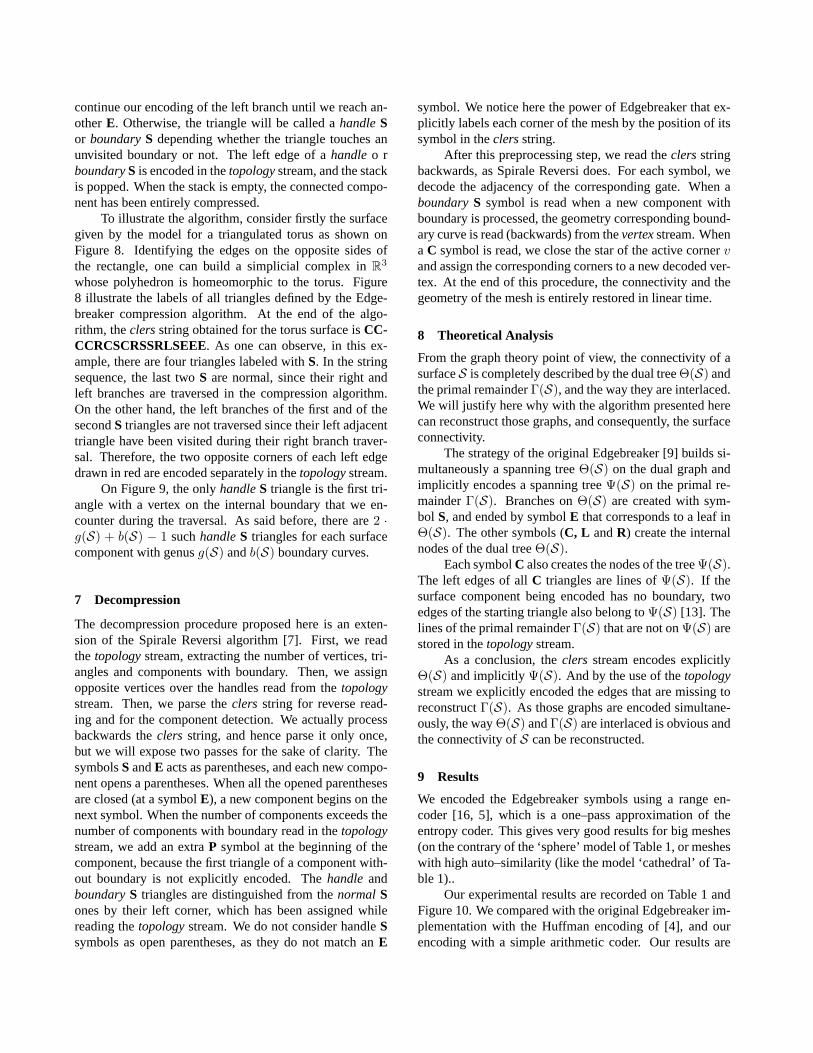
continue our encoding of the left branch until we reach an-otherE. Otherwise, the triangle will be called ahandleSor boundaryS depending whether the triangle touches anunvisited boundary or not. The left edge of ahandleo rboundaryS is encoded in thetopologystream, and the stackis popped. When the stack is empty, the connected compo-nent has been entirely compressed.

To illustrate the algorithm, consider firstly the surfacegiven by the model for a triangulated torus as shown onFigure 8. Identifying the edges on the opposite sides ofthe rectangle, one can build a simplicial complex inR3

whose polyhedron is homeomorphic to the torus. Figure8 illustrate the labels of all triangles defined by the Edge-breaker compression algorithm. At the end of the algo-rithm, theclersstring obtained for the torus surface isCC-CCRCSCRSSRLSEEE. As one can observe, in this ex-ample, there are four triangles labeled withS. In the stringsequence, the last twoS are normal, since their right andleft branches are traversed in the compression algorithm.On the other hand, the left branches of the first and of thesecondS triangles are not traversed since their left adjacenttriangle have been visited during their right branch traver-sal. Therefore, the two opposite corners of each left edgedrawn in red are encoded separately in thetopologystream.

On Figure9, the onlyhandleS triangle is the first tri-angle with a vertex on the internal boundary that we en-counter during the traversal. As said before, there are2 ·g(S) + b(S) − 1 suchhandleS triangles for each surfacecomponent with genusg(S) andb(S) boundary curves.

7 Decompression

The decompression procedure proposed here is an exten-sion of the Spirale Reversi algorithm [7]. First, we readthe topologystream, extracting the number of vertices, tri-angles and components with boundary. Then, we assignopposite vertices over the handles read from thetopologystream. Then, we parse theclers string for reverse read-ing and for the component detection. We actually processbackwards theclers string, and hence parse it only once,but we will expose two passes for the sake of clarity. ThesymbolsSandE acts as parentheses, and each new compo-nent opens a parentheses. When all the opened parenthesesare closed (at a symbolE), a new component begins on thenext symbol. When the number of components exceeds thenumber of components with boundary read in thetopologystream, we add an extraP symbol at the beginning of thecomponent, because the first triangle of a component with-out boundary is not explicitly encoded. ThehandleandboundaryS triangles are distinguished from thenormal Sones by their left corner, which has been assigned whilereading thetopologystream. We do not consider handleSsymbols as open parentheses, as they do not match anE

symbol. We notice here the power of Edgebreaker that ex-plicitly labels each corner of the mesh by the position of itssymbol in theclersstring.

After this preprocessing step, we read theclersstringbackwards, as Spirale Reversi does. For each symbol, wedecode the adjacency of the corresponding gate. When aboundaryS symbol is read when a new component withboundary is processed, the geometry corresponding bound-ary curve is read (backwards) from thevertexstream. Whena C symbol is read, we close the star of the active cornervand assign the corresponding corners to a new decoded ver-tex. At the end of this procedure, the connectivity and thegeometry of the mesh is entirely restored in linear time.

8 Theoretical Analysis

From the graph theory point of view, the connectivity of asurfaceS is completely described by the dual treeΘ(S) andthe primal remainderΓ(S), and the way they are interlaced.We will justify here why with the algorithm presented herecan reconstruct those graphs, and consequently, the surfaceconnectivity.

The strategy of the original Edgebreaker [9] builds si-multaneously a spanning treeΘ(S) on the dual graph andimplicitly encodes a spanning treeΨ(S) on the primal re-mainderΓ(S). Branches onΘ(S) are created with sym-bol S, and ended by symbolE that corresponds to a leaf inΘ(S). The other symbols (C, L andR) create the internalnodes of the dual treeΘ(S).

Each symbolC also creates the nodes of the treeΨ(S).The left edges of allC triangles are lines ofΨ(S). If thesurface component being encoded has no boundary, twoedges of the starting triangle also belong toΨ(S) [13]. Thelines of the primal remainderΓ(S) that are not onΨ(S) arestored in thetopologystream.

As a conclusion, theclers stream encodes explicitlyΘ(S) and implicitlyΨ(S). And by the use of thetopologystream we explicitly encoded the edges that are missing toreconstructΓ(S). As those graphs are encoded simultane-ously, the wayΘ(S) andΓ(S) are interlaced is obvious andthe connectivity ofS can be reconstructed.

9 Results

We encoded the Edgebreaker symbols using a range en-coder [16, 5], which is a one–pass approximation of theentropy coder. This gives very good results for big meshes(on the contrary of the ‘sphere’ model of Table1, or mesheswith high auto–similarity (like the model ‘cathedral’ of Ta-ble1)..

Our experimental results are recorded on Table1 andFigure10. We compared with the original Edgebreaker im-plementation with the Huffman encoding of [4], and ourencoding with a simple arithmetic coder. Our results are

Model |V(S)| |T (S)| Dum Ori Ours Ori/Ours Dum/Ourssphere 1 848 926 3.39 3.39 3.45 0.98 0.98violin 1 508 1 498 3.16 2.21 2.25 0.98 1.41pig 3 560 1 843 3.26 3.24 3.13 1.03 1.04rose 3 576 2 346 3.37 2.95 2.64 1.12 1.28cathedral 1 434 2 868 2.25 1.00 0.19 5.27 11.86blech 7 938 4 100 3.25 3.18 2.40 1.33 1.35mask 8 288 4 291 3.19 3.12 1.93 1.62 1.65skull 22 104 10 952 3.51 3.51 3.30 1.06 1.06bunny 29 783 15 000 3.36 3.34 1.27 2.62 2.64terrain 32 768 16 641 3.03 3.00 0.40 7.43 7.51david 47 753 24 085 3.45 3.85 3.07 1.25 1.12gargoyle 59 940 30 059 3.28 3.27 2.11 1.55 1.55

Table 1: Comparative results on different models (drawn on Figure10). ‘Dum’ stands for the dummy vertex method toencode meshes with boundaries [4], and ‘Ori’ stands for the original Edgebreaker [9], and ‘Ours’ for the algorithm introducedhere. The size of the compressed symbols (columns ‘Dum’, ‘Ori’ and ‘Ours’) is expressed in bit per vertex. Our algorithm hasa compression ration in weighted average 2.5 better than the other two. The ‘sphere’ model has the same encoding in all theabove algorithms, but the range coder used has a lower performance since there are few symbols to encode. The ‘cathedral’model is the output of an architecture modeling program, which is almost unstructured: all the connected components arepairs of triangles.

always better than the original Edgebreaker, mainly due tothe range encoder. However, the entropy of our codes is al-ways better than the other implementations of Edgebreaker(see Figure10(b)).

(a) Size of the compressed file vscomplexity of the model.

(b) Entropy vs complexity of themodel.

Figure 10:Comparison of the final size and of the entropyof the Edgebreaker’s symbols: for the range encoder, thoseparameters depends more on the regularity than on the sizeof the model, but our algorithm really enhance the previousresults.

10 Conclusion

We introduced here a simple, efficient and robust algorithmto code and decode the connectivity of an orientable mani-fold surface. The compression scheme is based on Edge-breaker, although we use only the 5 original symbols toencode topological features, maintaining explicit labelingof vertices and the ability to use a geometric predictiveencoding. The decompression scheme is an extension ofSpirale Reversi, which ensures a linear complexity and a

one-pass decompression complexity. This guarantees lessthan 2 bits per triangle connectivity compression, with a2 · log2(|T (S)|) bits over-cost for each half handle and foreach boundary curve, and bests previous Edgebreaker’s en-coding for surfaces with boundaries. Moreover, the use of arange encoder significantly improves the final compressionresults.

References

[1] M. Armstrong. Basic topology. McGraw-Hill, Lon-don, 1979.

[2] L. Glaser.Geometrical Combinatorial Topology. VanNostrand Reinhold, New York, 1970.

[3] P. Alliez and M. Desbrun. Valence-Driven Connec-tivity Encoding of 3D Meshes. In Eurographics 2001Conference Proceedings, pages 480–489, 2001.

[4] D. King and J.Rossignac. Guaranteed 3.67V Bit En-coding of Planar Triangle Graphs. In Canadian Con-ference on Computational Geometry, pages 146–149,1999.

[5] M. Schindler. Range encoder.www.compressconsult.com/rangecoder.

[6] C. Toumaand C.Gotsman. Triangle Mesh Compres-sion. In Graphics Interface, pages 26–34, 1998.

[7] M. Isenburgand J.Snoeyink. Spirale Reversi: Re-verse decoding of the Edgebreaker encoding. InCanadian Conference on Computational Geometry,pages 247–256, 2000.

[8] A. Gueziec, F. Bossen, G. Taubin, and C. Silva.Efficient Compression of Non-Manifold PolygonalMeshes. Computational Geometry: Theory and Ap-plications, 14(1–3):137–166, 1999.

[9] J.Rossignac. Edgebreaker: Connectivity compressionfor triangle meshes. IEEE Transactions on Visualiza-tion and Computer Graphics, 5(1):47–61, 1999.

[10] J. Rossignac, A. Safonova, and A. Szymczak.3D Compression Made Simple: Edgebreaker on aCorner-Table. In Proceedings of the 2001 Shape Mod-eling International Conference, 2001.

[11] J.Rossignacans AndrzejSzymczak. Wrap & Zip de-compression of the connectivity of triangle meshescompressed with Edgebreaker. Computational Ge-ometry: Theory and Applications, 14(1–3):119–135,1999.

[12] D. Poulalhonand G.Schaeffer. Optimal Coding andSampling of Triangulations. In ICALP, pages 1080–1094, 2003.

[13] H. Lopes, J. Rossignac, A. Safonova, A. Szymczak,and G.Tavares. Edgebreaker: a simple implementa-tion for surfaces with handles. Computers & Graph-ics, 27(4), 2003.

[14] G. Taubinand J.Rossignac. Geometric compressionthrough topological surgery. ACM Transactions onGraphics, 17(2):84–115, 1998.

[15] B. Kronrod and C.Gotsman. Efficient Coding ofNontriangular Mesh Connectivity. Graphical Models,63:263–275, 2001.

[16] G. Martin. Range encoding: an algorithm for remov-ing redundancy from a digitised message. In Video &Data Recoding Conference, 1979.

[17] D. Salomon.Data Compression: The Complete Ref-erence, 2nd Edition. Springer Verlag, Berlim, 2000.

(a) violin (135 comps,138 bdries)

(b) pig (6 bdries)

(c) rose (51 comps, 64bdries, genus 1)

(d) cathedral (717comps)

(e) blech (f) mask (7 bdries)

(g) skull (genus 51) (h) bunny (5 bdries)

(i) terrain (j) david

(k) gargoyle

Some of the modelsused for the experi-ments, with the be-ginning of the dualspanning tree gener-ated by Edgebreaker.