efficient detection algorithms for mimo channels: a

2808 IEEE TRANSACTIONS ON SIGNAL PROCESSING, VOL. 51, NO. 11, NOVEMBER 2003

Efficient Detection Algorithms for MIMOChannels: A Geometrical Approach to

Approximate ML DetectionHarold Artés, Student Member, IEEE, Dominik Seethaler, Student Member, IEEE, and

Franz Hlawatsch, Senior Member, IEEE

Abstract—It is well known that suboptimal detection schemesfor multiple-input multiple-output (MIMO) spatial multiplexingsystems (equalization-based schemes as well as nulling-and-can-celling schemes) are unable to exploit all of the available diver-sity, and thus, their performance is inferior to ML detection. Mo-tivated by experimental evidence that this inferior performance isprimarily caused by the inability of suboptimal schemes to dealwith “bad” (i.e., poorly conditioned) channel realizations, we studythe decision regions of suboptimal schemes for bad channels. Basedon a simplified model for bad channels, we then develop two com-putationally efficient detection algorithms that are robust to badchannels. In particular, the novelsphere-projection algorithm(SPA)is a simple add-on to standard suboptimal detectors that is able toachieve near-ML performance and significantly increased diver-sity gains. The SPA’s computational complexity is comparable withthat of nulling-and-cancelling detectors and only a fraction of thatof the Fincke–Phost sphere-decoding algorithm for ML detection.

Index Terms—Equalization, maximum likelihood detection,MIMO channels, nulling and cancelling, spatial multiplexing,sphere decoding, V-BLAST.

I. INTRODUCTION

M ULTIPLE-INPUT multiple-output (MIMO) fadingchannels offer not only the potential of high data rates

but also the promise of high reliability due to their inherentlyavailable diversity (e.g., [1]). It is well known that this availablediversity cannot be fully exploited by suboptimal equalization-based detection schemes (e.g., [2]), including nulling-and-cancelling schemes [3]. Maximum-likelihood (ML) detectioncan exploit all of the available diversity but tends to be com-putationally intensive. This is also true for the Finke–Phostsphere-decoding ML algorithm [4], as will be illustrated inSection VII. Thus, there is a strong demand for computationallyefficient suboptimal detection algorithms that can exploit alarge part of the available diversity.

In this paper, we develop such improved detection algorithmsfor spatial multiplexing systems such as V-BLAST [2]. Ourstarting point is to examine why the suboptimal detection

Manuscript received December 20 2002; revised April 22, 2003. This workwas supported by the FWF under Grant P15156. The associate editor coordi-nating the review of this paper and approving it for publication was Dr. Rick S.Blum.

The authors are with the Institute of Communications and Radio-FrequencyEngineering, Vienna University of Technology, A-1040 Wien, Austria (e-mail:[email protected]).

Digital Object Identifier 10.1109/TSP.2003.818210

schemes fail to exploit all of the available diversity. One ex-planation is that suboptimal detection “uses up” the degrees offreedom that would otherwise offer diversity (e.g., [5]). Here,we explain the inferior performance of suboptimal detectionschemes by comparing the decision regions of these schemesto the decision regions of the ML detector. The “improper”decision regions of suboptimal schemes are no problem forchannel realizations with a condition number near to 1. (Notethat for condition number 1, zero-forcing equalization followedby componentwise quantization is equivalent to ML detection.)However, for channel realizations with a large conditionnumber, they cause a significant performance degradation. Infact, it turns out that these “bad”1 channel realizations withlarge condition number are to a great extent responsible for theinferior average performance of suboptimal detection.

Motivated by this insight, we introduce an idealized modelfor bad channels that allows a substantially simplified imple-mentation of ML detection. This efficient detection algorithmis then extended to nonidealized channels. A final modificationand simplification yields the novelsphere-projection algorithm(SPA). The SPA is an efficient nonlinear add-on to standard sub-optimal detection schemes that makes these schemes robust tobad channels. For spatial multiplexing systems of pratical in-terest (e.g., six transmit antennas and six receive antennas), thedetection schemes obtained by this approach are demonstratedto yield excellent performance at low computational complexity.

Our paper is organized as follows. In the remainder of thissection, we describe the system model and give an overviewof existing detection schemes for spatial multiplexing systems.In Section II, the effects of bad channels on equalization-baseddetection schemes are discussed. An idealized model for badchannels is introduced in Section III, and an efficient ML detec-tion algorithm for this model is developed in Section IV. In Sec-tion V, this detection algorithm is extended to arbitrary MIMOchannels (for which it will no longer be ML). In Section VI, asimplification of this latter detection algorithm yields the SPA.Finally, simulation results presented in Section VII show thatthe proposed algorithms can yield near-ML performance at justa fraction of the computational cost of the Fincke–Phost sphere-decoding algorithm.

1The term “bad” refers to the poor performance of suboptimal detectionschemes for spatial multiplexing systems. Note, however, that these channelsare not necessarily “bad” in the sense of, e.g., low channel capacity.

1053-587X/03$17.00 © 2003 IEEE

IEEE Trans. Signal Processing, Special Issue on MIMO Wireless Communications, vol. 51, no. 11, Nov. 2003, pp. 2808–2820Copyright IEEE 2003

ARTÉSet al.: EFFICIENT DETECTION ALGORITHMS FOR MIMO CHANNELS 2809

Fig. 1. Detector performance and channel condition number for a (4,4), iidGaussian channel. (a) SER performance of various detection schemes versuscondition number of the respective channel realization for QPSK modulationand an SNR of 15 dB. (ZF is ZF equalization based detection, MMSE is MMSEequalization based detection, NC-MMSE is nulling and cancelling using MMSEequalization, and ML is ML detection.) (b) Cumulative distribution function ofthe condition number.

A. System Model

We consider a MIMO channel with transmit antennasand receive antennas [this will be briefly termedan ( , ) channel]. This channel is part of a spatialmultiplexing system such as V-BLAST [2], where thethdata stream (orlayer) is directly transmitted on the thtransmit antenna. This leads to the well-known baseband model

(1)

with the transmit vector, the channel matrix , the re-

ceived vector , and the

noise vector . The datastreams are assumed zero-mean, uncorrelated, stationary,white random processes with variance. The channel isconsidered constant over a block of consecutive time instantsand perfectly known at the receiver. The noise processesare statistically independent, zero-mean, circularly symmetriccomplex-valued, Gaussian, stationary, white random processeswith variance . For simplicity, we will hereafter omit the timeindex and, thus, write (1) as .

B. Review of Detection Schemes for Spatial MultiplexingSystems

The major detection approaches for spatial multiplexing sys-tems are linear equalization followed by quantization (e.g., [2]),nulling and cancelling (or decision-feedback) [2], and ML de-tection [4], [6]. The first two approaches are suboptimal but havesignificantly lower computational complexity than ML detec-tion. We will briefly review these three detection schemes.

Linear Equalization Based Detection:In linear equaliza-tion-based detection, an estimate of the transmitted data vector

is calculated as , where is an equalization matrix.The detected data vector is then obtained as ,where denotes componentwise quantization accordingto the symbol alphabet used. (Componentwise quantization issuboptimal in general because the multiplication byintro-duces correlations of the noise components.) Thezero-forcing(ZF) equalizer is given by the pseudo-inverse [7] of, i.e.,

. (For the last expression, we

assumed that and that has full rank.) Thus, theresult of ZF equalization (before quantization) is

which is the transmitted data vector corrupted by thetransformed noise . The minimum mean-square error (MMSE) equalizer is given by [8]

, which minimizes the mean-squareerror . Thus, the result of MMSE equalization is

Nulling and Cancelling: In contrast to linear data detection,where all layers are detected jointly, nulling and cancelling (NC)uses a serial decision-feedback approach to detect each layerseparately (e.g., [2]). When a layer has been detected, an esti-mate of the corresponding contribution to the received vectoris subtracted from; the result is then used to detect the nextlayer, etc. In the absence of detection errors, NC progressivelycleans from the interference corresponding to the layers al-ready detected. To detect a specific layer, the layers that havenot been detected yet are “nulled out” (equalized) according tothe ZF or MMSE approach described above. Error propagationcan be a problem because incorrect data decisions actually in-crease the interference when detecting subsequent layers. Thus,the order in which the layers are detected strongly influencesthe performance of NC.

ML Detection: ML detection is optimal in the sense of min-imum error probability when all data vectors are equally likely.For our system model (1) and our assumptions, the ML detectoris given by

(2)

Here, denotes the set of all possible transmitted data vectors, . We note that , where is the el-

ementary symbol alphabet, and thus, . In general,the computational complexity of ML detection grows expo-nentially with . Using the Finke–Phost sphere-decodingalgorithm [4], ML detection can be achieved at anaveragecomplexity that increases with roughly as , aswas shown in [9]. However, for bad channel realizations,the complexity of sphere-decoding can be very high (seeSection VII-C).

It can be shown [4] that the ML decision rule (2) can berewritten as

(3)

This can be interpreted as the ML detector for anidentitychannel corrupted by zero-mean Gaussian noise(the noise contained in ) with covariance matrix

(4)

That is, after ZF equalization the noise is generallycorrelated.We may view (3) as “ML detection after ZF equalization” or


“ML detection in the ZF-equalized domain,” as opposed to “di-rect ML detection” according to (2). Note, however, that (2) and(3) are strictly equivalent.

II. “B AD CHANNEL” EFFECT

In this section, we will demonstrate that the inferior perfor-mance of suboptimal detection compared with ML detection ismainly caused by the occurrence of bad channel realizations.

A. Detector Performance and Bad Channels

In what follows, we will use the singular value decomposition(SVD) , where the diagonal matrix contains thesingular values of and the matrices and contain,respectively, the left and right singular vectors ofas columns[7]. We assume that the are indexed in nonincreasing order.The condition number is the ratio of thelargest to smallest singular value. For a bad (poorly conditioned)channel, is large.

Experiments suggest that the performance of suboptimaldetection schemes strongly depends on the channel’s conditionnumber. In Fig. 1(a), we show the symbol error rate (SER) ofvarious detection schemes versus the condition number of thechannel realization. In this simulation, we used a (4,4) channelwith independent and identically distributed (iid) Gaussianchannel matrix entries, QPSK modulation, and an SNR of 15dB. It can be seen that there is a significant performance gapbetween linear (i.e., ZF or MMSE) detection and ML detectionfor about 4 or larger and between NC and ML detection for

about 20 or larger.The impact of this behavior on theaverageSER performance

of suboptimal detection of course depends on the probabilitywith which bad channels occur. In Fig. 1(b), we show the cumu-lative distribution function (cdf) of estimated in the courseof the simulation described above. It is seen that the probabilitythat exceeds a value of 10, 15, and 20 is 32%, 15%, and 9%,respectively. This suggests that bad channels occur frequentlyenough to cause a significant degradation of the average per-formance of suboptimal detection schemes. Theoretical inves-tigations show that for an increasing number of transmit andreceive antennas, the cdf is essentially scaled (expanded) in the

direction [10]. We can thus expect the bad channel effect tobecome even worse for an increasing number of antennas.

While the performance of ML detection is fairly robust tobad channel realizations, it is noteworthy that the computationalcomplexity of the Finke–Phost sphere-decoding algorithm forML detection significantly increases for bad channels [4], [11].Thus, there is a strong demand for computationally efficientsuboptimal detectors that are able to achieve near-ML perfor-mance. The detection methods presented in this paper are de-signed to satisfy this demand.

B. Geometrical Analysis

The starting point for developing these improved detectionmethods is a geometrical analysis of the decision regions of sub-optimal detection methods in the case of bad channels.

ZF Detection: We first consider linear detection based on ZFequalization. For a perfectly conditioned channel, i.e., ,

Fig. 2. Probability density function ofy and ZF and ML decision regions inthe ZF-equalized domain for a real-valued (2,2) channel and BPSK modulation.(a) “Good” channel realization with condition number 1.3. (b) “Bad” channelrealization with condition number 7.1. The ZF decision regions are the fourquadrants; the ML decision regions are indicated by dash-dotted lines.

we have . Here, (4) shows that the components of thenoise vector are uncorrelated; furthermore, the MLdetector in (3) simplifies toand thus becomes equal to the ZF detector solution

. On the other hand, for a poorly conditioned channel,is quite different from being proportional to. Thus, the

components of are generally correlated, and the ZF solutionmust be expected to be far away from the op-

timal ML solution2 .For a geometrical analysis, we consider the probability den-

sity function (pdf) of the ZF-filtered Gaussian noise vector.The contour surfaces of this pdf are hyperellipsoids [12]. Using

, the covariance matrix canbe written as

The th principal axis of the hyperellipsoids is such that itsdirection is given by the th eigenvector of , which isequal to the th column of , and its length is proportionalto the square root of the th eigenvalue of [12], which isequal to

(5)

Thus, ZF equalization results in adistortion of the noise pdfwith respect to the spherical geometry of the pdf of the originalnoise vector .

For illustration, Fig. 2 shows the pdf of the received vectorafter ZF equalization for two different realizations of areal-valued (2,2) channel with condition numbers 1.3 and 7.1.The modulation format is BPSK. This figure also shows the ZFdecision regions (the four quadrants) and the ML decision re-gions (indicated by dash-dotted lines). Whereas the ZF and MLdecision regions are similar for the “good” channel with con-dition number 1.3, they are dramatically different for the “bad”channel with condition number 7.1. Indeed, in the latter case,

2Note that even whenc > 1, it is possible thatH has orthogonal columnsbut with different norms. In this case,H H is diagonal, which means that thecomponents of~w are still uncorrelated, and ZF detection will still be optimal.However, simulations show that for poorly conditioned channel realizations, asituation close to this case is very unlikely.


Fig. 3. Same as Fig. 2(b) but with (a) MMSE decision regions and (b) ZF-based NC decision regions instead of ML decision regions. The boundaries ofthe MMSE and NC decision regions are indicated by dash-dotted lines.

the ML decision regions are nicely matched to the distortednoise pdf, but the ZF decision regions are not because they cor-respond to simple componentwise quantization. In particular,the boundary lines of the ML decision regions differ mainly byoffsets that are orthogonal to the dominant principal axis(corresponding to the dominant eigenvalue of and,thus, to the dominant noise component). This is intuitive, sinceany shift in the received vector in the direction of the dominantnoise component is very likely caused by noise. For bad chan-nels, it is thus desirable that the decision regions be approxi-mately invariant to shifts in the direction of the dominant prin-cipal axis . In general, the decision regions of linear detec-tion schemes cannot have this property because their boundarylines always go through the origin.

MMSE Detection:Fig. 3(a) shows the decision regions ofMMSE equalization-based detection in the ZF equalized do-main3 for the bad channel realization (condition number 7.1).The angles of the boundary lines of the MMSE decision regionsare better matched to the distorted noise pdf than those of the ZFdecision regions; however, the boundary lines still go throughthe origin and, thus, cannot implement the offsets that wouldallow them to become similar to the ML decision regions.

NC Detection: Finally, Fig. 3(b) shows the decision regions(again represented in the ZF equalized domain) for ZF-basedNC detection. Because the first symbol is simply ZF detected,one boundary of the corresponding decision region is fixed tothe ordinate, which is again quite different from the ML decisionregions. For successive symbols, offsets can be realized only toa certain extent. As a consequence, ZF-based NC detection per-forms better than ZF or MMSE detection but is still significantlypoorer than ML detection. For MMSE-based NC detection, asimilar argument applies. Fig. 1(a) shows that for growing,the performance gap betwen MMSE-based NC detection andML detection increases more slowly than that of ZF or MMSEdetection but eventually becomes just as wide as that of MMSEdetection.

Furthermore, it can be shown that the diversity gain achievedby NC (both ZF- and MMSE-based) is given by[3]. Thus, for , the diversity gain is small.

3We represent and compare the decision regions of all detectors in a commondomain, namely, the domain obtained after ZF equalization. Note that ZF equal-ization by itself does not imply any loss of optimality, and it has the advantagethat the symbols are at the correct positions.

Fig. 4. Ratio of noise variances� =� in the direction of consecutiveprincipal axes in the ZF-equalized domain and channel condition numberc .(a) Average ratiosEf� =� g versus the condition numberc of therespective channel realization for a (4,4) iid Gaussian channel. (b) cdf of theratios� =� for c = 70.

III. I DEALIZED BAD CHANNEL MODEL

The previous results suggest that the average performanceof suboptimal detection schemes can be improved by makingthese schemes robust to bad channels. Specifically, the decisionregions should be made approximately invariant to a shift inthe direction of the dominant noise axis. As a basis for such amodification, we will first formulate an idealized model for badchannels. In Section IV, this will allow us to derive an efficientnear-ML detection algorithm for bad channels.

A. Formulation of the Idealized Bad Channel Model

Our idealized bad channel model can be motivated as fol-lows. According to (5), i.e., , the ratios of thenoise variances in the directions of consecutive principal axesare given by . Fig. 4(a) shows es-timates of theaverageratios for a (4,4) channelwith iid, circularly symmetric complex-valued, Gaussian entriesversus (i.e., the were estimated byaveraging over an ensemble of channels with a given

). It can be seen that for a bad channel (i.e., large), on av-erage, is much larger than the other ratios and

. Thus, on average, is much smallerthan the othersingular values , , , or equivalently, the largest prin-cipal-axis noise variance is much largerthan theother principal-axis noise variances , , and . Sim-ulations show that a similar behavior is also exhibited by higherdimensional channels. To demonstrate that the ratiosare well concentrated about their mean , Fig. 4(b)shows the cdf of for .

This suggests that for a bad channel, the largest noise vari-ance (corresponding to the smallest singular value ofand the associated principal axis ) dominates all the othernoise variances and, hence, causes the main part of the badchannel effects that plague suboptimal detection. Therefore,we approximate a bad channel by anidealized bad channelmodel (IBCM) that is constructed by setting the smallestsingular value equal to zero and the remaining singular valuesequal to the largest singular value:

with

and (6)


Note that whereas the singular vectors of the respectivechannel realization —and thus the principal axis directionsof the ZF-domain noise as well—are maintained, the prin-cipal-axis noise variances are modified because we use anin-finite dominant noise variance andequalremaining noise variances

for . (Actually, we will see presentlythat the values of these remaining noise variances do not matteras long as they are finite and equal.) Indeed, approximating achannel with the IBCM is equivalent to approximating thehyperellipsoids constituting the contour surfaces of the pdf ofby hypercylinders of infinite length whose axis is the dominantnoise axis . This approximation is motivated by our desireto make the decision regions invariant to a shift in the directionof , as described in Section II-B.

B. ML Detection for the Idealized Bad Channel Model

Although the IBCM is only a crude approximation to a badchannel , it does capture an essential part of the “bad channel”effects that plague suboptimal detection. We now consider MLdetection for the IBCM (termedIML detection); this will laterserve as a basis for developing an efficient near-ML detector forbad channels. According to (3), the IML decision rule is

(7)

Using (6), we have

, with denoting the orthogonalprojector onto the space orthogonal to . Thus, (7) becomes

(8)

where we have used . Because of the pro-jector occurring in (8), the norm of the component of

perpendicular to is minimized, whereas the com-ponent of in the direction of (the dominant noisedirection) is suppressed in this minimization. Thus, as desired,the IML decision regions are invariant to this latter component.

For an alternative formulation and geometrical interpretationof the IML decision rule (8), let us define thereference line asthe straight line that is parallel to the dominant noise axisand whose offset from the origin is :

(9)

We maintain that the norm minimized in(8) is equal to the distance of from . Indeed, letdenote the point of closest to a given data vector, i.e.,

for. Then,

Fig. 5. Illustration of IML detection for a real-valued (2,2) channel and BPSKmodulation. (a) pdf ofy for the IBCM corresponding to the bad channelof Figs. 2 and 3 and IML decision regions indicated by dash-dotted lines. (b)Reference-line geometry of IML detection according to (10).

the distance of from is given by , and this dis-tance can easily be shown to be equal to :

Thus, as claimed,ML detection for the IBCM is equivalent tofinding the data vector that minimizes the distance

from the reference line :

(10)

This formulation will be essential for developing an efficientML detection algorithm in Section IV.

To continue the example of Figs. 2 and 3, Fig. 5(a) depictsthe pdf of for the IBCM associated with the bad channelrealization with . The IML decision regions are alsoshown. The geometry of the reference-line formulation of IMLdetection (10) is illustrated in Fig. 5(b).

IV. EFFICIENT ML DETECTOR FOR THE

IDEALIZED BAD CHANNEL MODEL

In this section, we develop an efficient ML detection algo-rithm with complexity for the IBCM. We first show thatthe reference-line formulation of the IML detector derived in theprevious subsection allows a significant reduction of the searchset .

A. Reduced Search Set

Let be the ZF decision region (in the ZF-equalized do-main) corresponding to a data vector . That is, forany , the ZF decision is . Because, in theZF-equalized domain, the ZF decision is a simple component-wise quantization, every is closer to than to anyother data vector . We will also say that is “thedata vector corresponding to .”

Theorem 1: The ML detector for the IBCM in (8) is equiva-lent to

(11)


where the reduced search set is given by all data vectorsthat correspond to ZF decision regions pierced by the

reference line in (9).Proof: As before, let denote the point of closest

to so that expresses the distance offrom .Assume (proof by contradiction) that doesnotcorrespondto a ZF decision region pierced by, i.e., no point of lies inthe ZF decision region of . Hence, in particular,does not lie in the ZF decision region of , and thus, it mustlie in the ZF decision region of some other data vector .That is, is closer to than to , i.e.,

. For this other data vector, we also have

because is the point of closest to , and thus,cannot be closer to . Combining the above two

inequalities yields ,which means that is closer to than , but we knowfrom (10) that is the data vector closest to. Thus, wehave a contradiction, and the proof is complete.

It will be advantageous to represent the complex referenceline , as an equivalentrealreference plane —the 2-D plane with

Re and Im . Replacing complex scalars by 2-Dvectors composed of the real and imaginary parts, theth scalarcomponent of the reference line equation, given by

, can be written as

(12)

with

The reduced search setthen consists of all data vectorswhose ZF decision regions are sliced by the real reference

plane (since slicing by is equivalent to piercing by ).To characterize , it is sufficient to specify for eachan arbitrary point of the decision region corresponding to,since can easily be recovered fromas . The ideabehind the algorithm proposed next is that these points can befound in the reference plane, and thus, the search for canbe restricted to .

B. Partitioning of the Reference Plane

The intersection of the ZF decision regions with the referenceplane induces a partitioning of . We will now show thatfor a wide class of symbol alphabets, this partitioning can becalculated very easily. Subsequently, this will serve as a basisfor an efficient determination of the reduced search set.

We assume a “line-structured” symbol alphabet, which, bydefinition, is such that the boundaries of the quantization re-gions in the 2-D real symbol domain (i.e., the ML decision re-gions for transmission of asinglesymbol over an additive whiteGaussian noise SISO channel) are given by straight lines. Exam-ples of line-structured alphabets are ASK, QAM, and PSK butnot, e.g., a hexagonal constellation. Letdenote the number of

Fig. 6. Boundary linesB in the real reference planeP for an (8,8)channel and 4-QAM modulation. (The boldface line segment will be addressedat a later point.)

boundary lines in the 2-D real symbol domain, and let thethreal boundary line be given by

(13)

with , where the 2 1 vectors and defineslope and offset, respectively. For example, the 4-QAM alphabet

has orthogonalboundary lines defined by , , and

.We now consider the partitioning of the reference plane

induced by the ZF decision regions. The ZF decision regionsare bounded by th hyperplanes. The (, ) hyperplane isobtained by setting the th component of a vector equal tothe th boundary line (13). To calculate the partitioning of,we must thus calculate the intersection ofwith all boundaryhyperplanes. The intersection ofwith the ( , )th boundaryhyperplane yields a straight boundary line that canbe calculated by equating (13) and (12), i.e., .This gives or, equivalently

(14)

with

where (note that. Because is an orthogonal matrix up to a factor,

the angles between the boundary lines corresponding to theth component are equal to the angles between the boundary

lines in the symbol alphabet domain.The boundary lines , ,

partition the reference plane into elementary cells. In Fig. 6, this cell partitioning of is illustrated for

an (8,8) channel and 4-QAM modulation; here, andso that we obtain boundary lines. Each cell

is the intersection of a ZF decision region with. Thus, allpoints of a given will lead to the same quantized data vector.More specifically, recall that each point of is parameterizedby or, equivalently, by , and


the corresponding vector in isin (9). Any point of a given cell corresponds to a vector

for which ZF decision (quantization) leads to the same, i.e., for all . This belongs to

the reduced search setbecause it corresponds to a ZF deci-sion region sliced by . Therefore,any collection of arbitrarycell points—one point for each cell—defines the reduced searchset . Note that the ZF estimate is obtained for

; see (9). Thus, belongs to thereduced search set.

From the above, it follows that the size of the reducedsearch set equals the number of cells. To find an upper boundon , recall that the cell partitioning is defined byboundary lines. Assuming that boundary lines are given,it is easy to verify that each additional boundary line yieldsat most new cells (it will yield new cells if and only if itintersects at different points with all previous lines). Thus

For example, for 4-QAM since there are no par-allel boundary lines, and only two boundary lines intersect ina given intersection point. If there are parallel boundary lines(e.g., 16-QAM) and/or if more than two boundary lines inter-sect in the same point (e.g., 8-PSK), then .

Comparing with , we see that for rea-sonably high data rates, . For example, for an (8,8)channel and 4-QAM modulation, we obtain

pierced decision regions out of a total ofdecision regions. This illustrates the significant reduction ofcomplexity achieved by the reduced search set.

We will next present an efficient algorithm for ML detectionthat is based on the reduced search setand the insights gainedso far. This algorithm consists of two parts: i) efficient determi-nation of and ii) efficient calculation of the distance of every

to the reference plane.

C. Efficient Determination of

According to the previous subsection, the reduced search setcan be determined by finding an arbitrary pointof each cell

since the corresponding defines the data vectorassociated with by . To find a point

of each cell in an efficient manner, we suggest a systematicsearch of the reference plane along each boundary line.

To search along the th boundary line , wecalculate the intersection points of withall , that are not parallel to .Equating with

and solving for yields

(15)

with

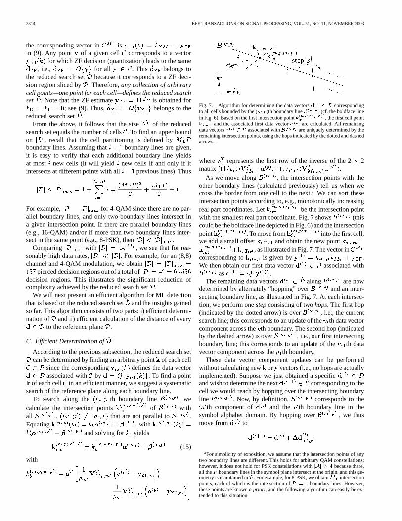
Fig. 7. Algorithm for determining the data vectorsd 2 ~D correspondingto all cells bounded by the (m,p)th boundary lineB (cf. the boldface linein Fig. 6). Based on the first intersection pointk , the first cell pointk and the associated first data vectord are calculated. All remainingdata vectorsd 2 ~D associated withB are uniquely determined by theremaining intersection points, using the hops indicated by the dotted and dashedarrows.

where represents the first row of the inverse of the 22matrix .

As we move along , the intersection points with theother boundary lines (calculated previously) tell us when wecross the border from one cell to the next.4 We can sort theseintersection points according to, e.g., monotonically increasingreal part coordinates. Let be the intersection pointwith the smallest real part coordinate. Fig. 7 shows (thiscould be the boldface line depicted in Fig. 6) and the intersectionpoint . To move from into the first cell,we add a small offset and obtain the new point

, as illustrated in Fig. 7. The vector incorresponding to is given by .We then obtain our first data vector associated with

as .The remaining data vectors along are now

determined by alternately “hopping” over and an inter-secting boundary line, as illustrated in Fig. 7. At each intersec-tion, we perform onestepconsisting of twohops. The first hop(indicated by the dotted arrow) is over , i.e., the currentsearch line; this corresponds to an update of theth data vectorcomponent across theth boundary. The second hop (indicatedby the dashed arrow) is over , i.e., our first intersectingboundary line; this corresponds to an update of theth datavector component across theth boundary.

These data vector component updates can be performedwithout calculating new or vectors (i.e., no hops are actuallyimplemented). Suppose we just obtained a specificand wish to determine the next corresponding to thecell we would reach by hopping over the intersecting boundaryline . Now, by definition, corresponds to the

th component of and the th boundary line in thesymbol alphabet domain. By hopping over , we thusmove from to

4For simplicity of exposition, we assume that the intersection points of anytwo boundary lines are different. This holds for arbitrary QAM constellations;however, it does not hold for PSK constellations withjAj > 4 because there,all theP boundary lines in the symbol plane intersect at the origin, and this ge-ometry is maintained inP . For example, for 8-PSK, we obtainM intersectionpoints, each of which is the intersection ofP = 4 boundary lines. However,these points are knowna priori, and the following algorithm can easily be ex-tended to this situation.


where the vector is zero except for the th com-

ponent. That component is given by an update valuethat depends on the th component of and on the thboundary. For example, for 4-QAM, we have

Im ifRe if

Thus, here, the update simply amounts to flipping the imaginarypart (for ) or the real part (for ) of the th datavector component.

D. Efficient Calculation of Distances

According to Theorem 1, we have to minimize the distanceover all . In the previous

subsection, we have shown how to determineefficiently. Wenow present an efficient recursive algorithm for calculating thesquared distances .

Again, we move along . Suppose that has alreadybeen determined and that the next data vector corre-sponds to a hop over the intersecting boundary line . Aswas shown in the previous subsection, is a neighbor of

that differs from only in the th component, namely,by . Thus, the distance for is

Re

(16)

with

Re (17)

where is the th component of and is the

th component of . This recursion is initial-ized by calculating in a straight-forward manner.

E. Summary of the ML Detection Algorithm

We have now developed the main elements of our efficientML detection algorithm for the IBCM. In an actual imple-mentation of this algorithm, the recursive procedure describedin Sections IV-C and D has to be performed for allboundary lines except for the last one (whose data vectors haveall been processed before) so that all data vectors aretaken into account and the ML solution according to (11) isobtained. For each boundary line, at most different datavectors are considered, which results in a total maximum of

checked data vectors. Comparedwith , we see that most ofthe data vectors are checked several times. (Of course,the distances for data vectors that have been checked before

Fig. 8. Processing associated with the(m;p)th boundary lineB .

need not be calculated anew.) For example, for an (8,8) channeland a 4-QAM alphabet, we have a maximum of 448 checkeddata vectors, of which maximally 137 are different. Note,however, that most of the multiply checked data vectors areobtained through efficient single symbol updates as describedabove.

The principal steps of our algorithm can finally be summa-rized as follows.

• Determine all boundary lines in [see (14)].• Calculate all intersection points (15) and order them for

each , e.g., according to increasing real part coor-dinates.

• For each , determine the associated data vectorsand their distances , as discussed in Sec-

tions IV-C and D. The processing associated withis summarized in Fig. 8.

V. EXTENSION TO ARBITRARY CHANNELS

The algorithm presented in the last section performs ML de-tection for the IBCM. Because actual channel realizations willnot conform to the IBCM, we will now extend our algorithm toan arbitrary MIMO channel . Specifically, we propose to usean IBCM approximation of to find the reduced search setand then to minimize over , i.e.,

Note that is notguaranteed to be equal to the ML decisionsince we minimize not over the whole data set

of size (which would have a computational complexitythat is exponential in ) but over the reduced set. On theother hand, the complexity of our algorithm is only , aswill be shown presently. The algorithm consists of the followingsteps.

• Calculate and .• Determine the dominant eigenvector of .• Using an IBCM approximation of , find the reduced

search set as explained in Section IV-C.


• Search for the data vector minimizing . Thesquared distances can again be cal-culated recursively; the update term in (17) is replacedby

Re (18)

where denotes the th column of . Here, the termcan be calculated recursively as well, and

the can be precalculated.Two cases where does coincide with are i) an or-

thogonal channel (here, and because

) and ii) an IBCM (here, ). Wecan thus expect near-ML performance for very good channelsand for bad channels with a single dominant noise axis.

For , we now study how the algorithm’s com-plexity depends on the parameters and that determinethe transmission rate. We first list the preparatory steps that haveto be performed once for each data block over which the channelis assumed constant, together with their complexity:

• calculation of and : com-plexity ;

• calculation of : complexity if the powermethod [7] is used;

• calculation of for : complexity.

Thus, the dominant complexity of the preparatory steps isper data block. Additionally, the following steps have

to be performed at each time instant (i.e., for each transmitteddata vector):

• determination of all boundary lines in and theirintersection points: complexity ;

• calculation of initial data vectors and their associ-ated distances: complexity ;

• calculation of roughly distance updatesaccording to (18): complexity .

Hence, theoverall complexityof our algorithm is pertransmitted data vector. This is cubic in the number of transmitantennas and, since usually , quadratic in thesymbol alphabet size .

VI. SPHERE-PROJECTIONALGORITHM

In this section, we will achieve another substantial reductionof computational complexity through a further reduction of thedata search set. The resulting sphere projection algorithm (SPA)can be viewed as a simple nonlinear add-on to an existing subop-timal scheme such as ZF, MMSE, or NC detection. This add-onimproves the error-rate and diversity-gain performance of thesuboptimal detector by making it robust to the bad channel ef-fects discussed in Section II.

The add-on construction of the SPA is as follows. Letdenote the result of the suboptimal detector. This result can beexpected to be reasonably good for a good channel. In orderto improve the performance for bad channels, we additionallyconsider a suitably chosen set of valid data vectors

that are potentially better than in the sense of smaller. We then minimize over the search set

that consists of and all data vectors in :

with

(19)The SPA is an add-on to the given suboptimal detector because

is calculated and included in the total search set.To keep our discussion simple, we consider only alphabets

with constant modulus (i.e., arbitrary PSK constellations,which includes 4-QAM and binary antipodal signaling). Here,all data vectors are located on an -dimensional “data hy-persphere” about the origin, with radius . Thisgeometry will allow a simple construction of that uses aprojection onto the data hypersphere(this explains the nameSPA). The SPA can be extended to symbol alphabets that do notsatisfy the constant-modulus property by using several hyper-spheres; however, this results in increased complexity.

A. Construction of the Additional Search Set

The additional search set has to be constructed such thatit improves the detector performance in the bad channel case.Therefore, let us consider a bad channel whose dominant noisecomponent in the direction of (i.e., of the reference line)is much larger than all other noise components. This channel canagain be approximated by an IBCM. Because the ML detectorfor the IBCM chooses the data vector with minimum distancefrom (see Section III-B), it makes sense to construct asa set of data vectors that are close to. On the other hand, weknow that all data vectors are located on the data hypersphere

. With the SPA, for reasons of algorithmic simplicity, we at-tempt to combine these two properties by choosing fordatavectors that are close to the intersection . However, thisintersection does not always exist. Therefore, two cases will bedistinguished.

• Case 1: If intersects , we choose to consist ofdata vectors located at or at least close to theintersection.

• Case 2: If does not intersect , we choose to consistof data vectors that are close to .

In the following, we will elaborate on both cases.Case 1: Suppose intersects . Using the decomposition

, where is col-inear with and is orthogonal to ,

can be rewritten as

with (20)

The intersection corresponds to the equationor, equivalently

(21)

In the real reference plane, is represented by the 2-D realvector , and . We can then write (21) as

(22)

with radius (note that

because we assumed that an intersection exists). Equa-


Fig. 9. Geometry underlying the SPA. (a) Some boundary lines intersect the intersection circleI (only possible for Case 1). (b) No boundary line intersectsI

(possible for Case 1 and Case 2). The shaded regions indicate (some of) the cells corresponding to data vectors inD .

tion (22) defines anintersection circle that representsin the reference plane. Because , the centerof is at .

Next, we find all cells that are pierced by theintersection circle . We first calculate all boundarylines . We then calculate the intersection points—ifthey exist—of each [see (14)] with [see (22)], i.e.,

, where is givenby (14). These intersection points are illustrated in Fig. 9(a).(Here, we assume that at least one boundary line intersects

. If no such intersection exists althoughintersects —cf.Fig. 9(b)—the processing for Case 2 described further belowhas to be performed.) The intersection points are sorted ac-cording to their angle. Starting with angle , the first datavector in is obtained as . Now, we movealong from one intersection point to the next one. In thisprocess, we apply the data component update procedure fromSection IV-C to obtain the remaining data vectors ,and we use the recursion (18) to efficiently calculate thedistances in (19).

The size of the resulting is bounded asbecause each one of the boundary lines has zero ortwo intersection points with . The worst caseoccurs if and only if all boundary lines intersect.

Case 2: If , then and do not intersect[see Fig. 9(b)]. It can here be shown that [which, ac-

cording to (20), corresponds to ] is the point of withminimum distance from . We thus take asthe first data vector in . Simulation results indicate that it isadvantageous to include also the nearest neighbors ofin

. These additional data vectors can easily be found by sub-stituting the nearest-neighbor symbols for the individual com-ponents of . For PSK constellations, we obtain two nearestneighbors for each data vector component, yielding

. The distances in (19) can againbe calculated recursively according to (18).

The same procedure is used if and intersect but noboundary line intersects the intersection circle (cf. thediscussion of Case 1 above).

B. Discussion of the Sphere-Projection Algorithm

Having explained the efficient construction of the additionalsearch set , we now discuss the use of the SPA5 as an add-onto a suboptimal detector.

Algorithm Summary and Complexity:The principal steps ofthe SPA can be summarized as follows.

• Calculate (the result of the given suboptimal de-tector) and the associated distance .

• Calculate and .• Calculate the dominant eigenvector of .• Calculate all boundary lines in .• Determine the additional search set and calculate the

corresponding distances— by considering all data vectors whose cells arepierced by the intersection circle;— or, if does not exist or if no boundary line inter-sects , by considering and its nextneighbors.

• Find the minimal distance (including the distance obtainedfor ).

Here, may be the result of ZF detection, MMSE detec-tion, ZF-based NC detection, or MMSE-based NC detection; theresulting SPA variants will be referred to as ZF/SP, MMSE/SP,NC-ZF/SP, and NC-MMSE/SP detection, respectively.

The computational complexity of the SPA add-on (notcounting calculation of ) can be estimated as follows.Among the preparatory steps that have to be performed oncefor each transmitted data block during which the channelis constant, calculation of has the dominantcomplexity of . Additionally, at each time instant, wehave to compute two distances with complexity and,in the worst case, efficient distance updates withtotal complexity . An experimental assessment ofcomplexity will be provided in Section VII-C.

5In both Case 1 and Case 2, an important aspect of the SPA is that we lookfor the point(s) on the data hypersphereH that is/are closest to the referencelineL. In a certain sense, this corresponds to a projection onto the hypersphereH, which explains the name “sphere-projection algorithm.” In Case 1, whereL

andH intersect, the projection points are given by the intersection circleI.


SPA Variants: To use the SPA as an add-on to ZF detection,we choose . The resultingZF/SP algorithmisthe most efficient SPA variant because calculation of is apart of the SPA.

To use the SPA as an add-on to MMSE detection, wechoose , where

is the result of MMSE equalization. Fur-thermore, we propose to replace the reference linein (20)by the “MMSE-based reference line” :

. is again parallel to the dominant principalaxis , but its offset is the component of (ratherthan of ) perpendicular to . The resultingMMSE/SPalgorithm can be obtained simply by replacing in the ZF/SPalgorithm with . The ratio-nale for the MMSE/SP algorithm is that on average,will be closer to the transmitted data vector than . Notethat applying the power method toinstead of requires a few more iterations to obtainaccurate results for . This is because the “regularizationterm” decreases the ratio of the largest to secondlargest singular value of , as comparedwith , which slows down the convergence of thepower method [7].

Finally, to combine the SPA with NC detection (eitherZF-based or MMSE-based), we propose to execute the ZF/SPor MMSE/SP algorithm, respectively, except for the use ofthe NC detection result for . As we will demonstratein Section VII, the NC-MMSE/SP algorithm is able to yieldvery-near-to-ML performance at a fraction of the computationalcost of Fincke and Phost’s sphere-decoding algorithm.

VII. SIMULATION RESULTS

Finally, we present simulation results in order to assessthe error-rate performance and computational complexity ofthe proposed detection algorithms in comparison to the ZF,MMSE, NC, and ML schemes. In our simulations, we used4-QAM modulation and MIMO channels with iid Gaussianentries. The dominant noise axis was computed by meansof the power method [7].

A. SER versus Number of Power Method Iterations

First, we study the dependence of the symbol error rate (SER)on the number of power method iterations, which is denoted by

. Fig. 10 shows the SER versus for ZF/SP and MMSE/SPdetection for a (6,6) channel at an SNR6 of 20 dB. For com-parison, the SER achieved with ZF and MMSE detection is in-dicated by horizontal lines. It is seen that for , the SPAadd-on yields significant performance improvements. For, we used a randomly chosen ; as can be expected, in this

case, the performance improvements yielded by the SPA add-onare negligible. For both ZF/SP and MMSE/SP, increasingbe-yond 4 does not yield any additional performance improvement.Thus, we chose in all simulations presented below.

6The SNR is defined asEfjjHdjj g=Efjjwjj g =M � =� .

Fig. 10. SER versus the number of power method iterationsK for a (6,6)channel and 4-QAM modulation at an SNR of 20 dB.K = 0 corresponds to arandomly chosen axisv .

(a)

(b)

Fig. 11. SER versus SNR performance of the various proposed and standarddetectors using 4-QAM modulation. (a) (4,4) channel. (b) (6,6) channel.

B. SER versus SNR

Figs. 11(a) and (b) show the SER versus SNR performance ofthe various proposed and standard detectors for a (4,4) channeland a (6,6) channel, respectively. As in Section V,ML denotesthe extension of the IML algorithm to arbitrary channels. For theNC algorithms, we used the layer ordering maximizing the post-


TABLE IMEASURED COMPLEXITY IN KFLOPS FOR(a) PREPARATORY (OVERHEAD) OPERATIONSPERFORMED ONCE PERDATA BLOCK AND

(b) DATA DETECTION OPERATIONSPERFORMEDONCE PERDATA VECTOR

detection signal-to-noise ratio at each detection step as proposedin [2]. The following conclusions can be drawn from the resultsshown in Fig. 11.

• All proposed detectors perform substantially better thanthe standard suboptimal detectors. In particular, even thesimplest of the proposed detectors (ZF/SP) outperformsthe best standard suboptimal detector (NC-MMSE withoptimal layer ordering).

• All proposed detectors achieve higher diversity ordersthan the standard suboptimal detectors.

• For the (4,4) channel, the MMSE/SP and NC-MMSE/SPdetectors perform practically as well as the ML detector[the corresponding SER curves in Fig. 11(a) are indistin-guishable], and the ZF/SP detector achieves near-ML per-formance.

• For the (6,6) channel, the NC-MMSE/SP detector achievesnear-ML performance, and the performance of the otherproposed detectors is intermediate between that of the MLdetector and that of the best standard suboptimal detector(NC-MMSE with optimal layer ordering).

• For the (6,6) channel, the performance of the ZF/SP andMMSE/SP detectors is close to that of the detector.This shows that our strategy for constructing workswell.

• A comparison of the results obtained for the (4,4) and (6,6)channels suggests that for increasing channel size, the per-formance of the proposed algorithms degrades (comparedwith ML performance). This is due to the IBCM approx-imation underlying our algorithms. Specifically, for in-creasing channel size, the probability that two or moreprincipal axes are dominant (rather than just one as as-sumed in the IBCM) increases so that the IBCM approxi-mation becomes less accurate.

C. Computational Complexity

A rough picture of the computational complexity of the var-ious detectors is provided in Table I for three different chan-nels [(4,4), (6,6), and (8,8)] and 4-QAM modulation. The kflopestimates displayed in Table I were measured using MATLABV5.3. Even though these complexity measurements depend onthe specific algorithm implementations used, they provide moreinsight than the asymtotic results presented in earlier sec-tions. The ML detector was implemented by means of Fincke

and Phost’s sphere-decoding (FPSD) algorithm [4]. The com-plexity of FPSD was measured at an SNR of 10 dB. The com-plexity of the other schemes is independent of the SNR.

Table I(a) shows the complexity of the operations that haveto be performed once for an entire data block during which thechannel is constant (i.e., “overhead” operations like calculationof and ). Table I(b) shows the com-plexity of the operations that have to be performed once foreach time instant or data vector (i.e., data detection operationslike determination of and , not including the overheadcomputations considered in Table I(a)). Each table presents onlyone value for both linear detectors (ZF and MMSE; denoted as“lin.”) and only one value for both linear detectors combinedwith the SPA (ZF/SP and MMSE/SP; denoted as “lin./SP”) be-cause there is virtually no difference in complexity. Note thatin Table I(a), the values for FPSD and lin. are equal since bothalgorithms have the same overhead complexity (computation of

). Similarly, in addition, the values forML and lin./SP areequal (same overhead of calculating and ).

The complexity of FPSD strongly depends on the channelrealization and the SNR; for a bad channel realization, it exceedsthe average complexity by a large amount. Thus, in addition tothe average FPSD complexity, Table I(b) shows the maximumFPSD complexity obtained during 10 000 simulation runs at anSNR of 10 dB. A maximum complexity is also provided forlin./SP and NC/SP; it refers to the case where all boundary linesintersect the intersection circle(cf. Case 1 in Section VI-A).

From Table I, the following conclusions can be drawn.

• The maximum complexity of FPSD is much larger thanits average complexity. For practical system design, a lim-itation of the maximum complexity is desirable. However,FPSD with limited maximum complexity is no longer anexact implementation of ML decoding.

• In contrast to FPSD, the complexity ofML detection isindependent of the channel realization and the SNR. Ac-cording to Table I(b), the complexity ofML detection issmaller than the average complexity of FPSD and only afraction of the maximum complexity of FPSD.

• For both FPSD andML, the complexity of the operationsto be performed in each time instant is much larger thanfor the other algorithms.

• For the lin./SP detectors, the complexity of the computa-tions performed once per data block is lower than for the


NC detectors but slightly higher than for the linear detec-tors and FPSD (due to the additional calculation of ).

• For the lin./SP detectors, the average complexity of thecomputations performed once per data vector is abouttwice that of the NC detectors but significantly lower (bya factor of about 25 33) than that of FPSD.

• The overall complexity of the SPA detectors is higher thanthat of the standard suboptimal detectors but much lowerthan that of FPSD and . In particular, the complexityof NC-MMSE/SP is just a fraction of the complexity ofboth FPSD and , even though NC-MMSE/SP achievesnear-ML performance, as shown in Section VII-B.

VIII. SUMMARY AND CONCLUSIONS

The starting point of this paper was an analysis of the effectsof bad (poorly conditioned) channels on suboptimal detectorsfor a MIMO spatial multiplexing system. The performance of allstandard suboptimal detection schemes severely degrades com-pared to the performance of the maximum-likelihood (ML) de-tector when bad channel realizations occur. We found that thisinferior performance is due to the inability of linear detectorsto properly adapt their decision regions to the noise statistics.In addition, bad channels lead to a high computational com-plexity of Fincke and Phost’s sphere-decoding algorithm for MLdetection.

Based on an idealized approximate model for bad channelsthat captures the bad channel effects in a simplified form, wethen presented new detection methods that are robust to badchannels. The initial form of the new detection approach wasan efficient ML detector for the idealized bad channel model.Subsequently, we extended this detector to be suitable forarbitrary (nonidealized) channels. Finally, we developed thesphere-projection algorithm(SPA) that is a computationally ef-ficient, nonlinear add-on to standard suboptimal detectors. Thisadd-on improves the error-rate and diversity-gain performanceof suboptimal detectors by making them robust to bad channelrealizations.

Simulations showed that the SPA outperforms ZF-basedand MMSE-based nulling and cancelling with optimal layerordering by achieving higher diversity gains at a comparablecomputational complexity. The performance of the SPA is bestfor systems of moderate size (which are of greatest practicalinterest), whereas for increasing system size, it degrades com-pared with the performance of ML detection. For example, fora spatial multiplexing system with six transmit antennas and sixreceive antennas, the SPA is able to yield near-ML performanceat just a fraction of the computational complexity of Fincke andPhost’s sphere-decoding algorithm for ML detection.

REFERENCES

[1] V. Tarokh, N. Seshadri, and A. R. Calderbank, “Space-time codes forhigh data rate wireless communications: performance criterion and codeconstruction,”IEEE Trans. Inform. Theory, vol. 44, pp. 744–765, Mar.1998.

[2] P. W. Wolniansky, G. J. Foschini, G. D. Golden, and R. A. Valenzuela,“V-BLAST: an architecture for realizing very high data rates over therich-scattering wireless channel,” inProc. URSI Int. Symp. Signals,Syst., Electron., Sept. 1998, pp. 295–300.

[3] W.-J. Choi, R. Negi, and J. Cioffi, “Combined ML and DFE decodingfor the V-BLAST system,” inProc. IEEE Int. Conf. Commun., NewOrleans, LA, June 2000, pp. 18–22.

[4] U. Fincke and M. Phost, “Improved methods for calculating vectorsof short length in a lattice, including a complexity analysis,”Math.Comput., vol. 44, pp. 463–471, Apr. 1985.

[5] L. Zheng and D. Tse, “Diversity and freedom: a fundamental tradeoff inmultiple antenna channels,”IEEE Trans. Inform. Theory, submitted forpublication.

[6] S. M. Kay, Fundamentals of Statistical Signal Processing: DetectionTheory. Upper Saddle River, NJ: Prentice-Hall, 1998.

[7] G. H. Golub and C. F. Van Loan,Matrix Computations, 3rded. Baltimore: Johns Hopkins Univ. Press, 1996.

[8] S. M. Kay, Fundamentals of Statistical Signal Processing: EstimationTheory. Englewood Cliffs, NJ: Prentice-Hall, 1993.

[9] B. Hassibi and H. Vikalo, “On the expected complexity of sphere de-coding,” in Proc. 35th Asilomar Conf. Signals, Syst., Comput., PacificGrove, CA, Nov. 2001, pp. 1051–1055.

[10] A. Edelman, “Eigenvalues and condition numbers of random matrices,”Ph.D. dissertation, Mass. Inst. Technol., Cambridge, MA, 1989.

[11] M. Damen, A. Chkeif, and J. Belfiore, “Lattice code decoder forspace-time codes,”IEEE Commun. Lett., vol. 4, pp. 161–163, May2000.

[12] C. W. Therrien,Discrete Random Signals and Statistical Signal Pro-cessing. Englewood Cliffs, NJ: Prentice-Hall, 1992.

Harold Artés (S’98) received the Dipl.-Ing. degreein electrical engineering from Vienna University ofTechnology, Vienna, Austria, in 1997, where he iscurrently pursuing the Ph.D. degree.

He is a Research (and partly Teaching) Assis-tant with the Institute of Communications andRadio-Frequency Engineering, Vienna Universityof Technology. He participated in the EuropeanCommission funded IST project ANTIUM andco-authored two patents. His research interestsinclude MIMO wireless communications, blind esti-

mation and equalization of time-varying channels, and multiuser techniques.

Dominik Seethaler (S’03) received the Dipl.-Ing.degree in electrical engineering from ViennaUniversity of Technology, Vienna, Austria, in 2002,where he is pursuing the Ph.D. degree.

He currently holds a Research and Teaching As-sistant position with the Institute of Communicationsand Radio-Frequency Engineering, Vienna Univer-sity of Technology. His research interests are in wire-less communications with emphasis on MIMO andmultiuser techniques.

Franz Hlawatsch (S’85–M’88–SM’00) receivedthe Dipl.-Ing., Dr. techn., and habilitation degrees inelectrical engineering/signal processing from ViennaUniversity of Technology, Vienna, Austria, in 1983,1988, and 1996, respectively.

Since 1983, he has been with the Institute ofCommunications and Radio-Frequency Engineering,Vienna University of Technology, where he currentlyholds an Associate Professor position. He wasa consultant for Schrack AG from 1983 to 1988and for AKG GesmbH from 1984 to 1985. From

1991 to 1992, he spent a sabbatical year with the Department of ElectricalEngineering, University of Rhode Island, Kingston. From 1999 to 2001, heheld one-month Visiting Professor positions with INP/ENSEEIHT, Toulouse,France, and IRCCyN, Nantes, France. He authored the bookTime-FrequencyAnalysis and Synthesis of Linear Signal Spaces(Boston, MA: Kluwer, 1998)and co-edited the bookThe Wigner Distribution—Theory and Applications inSignal Processing(Amsterdam, The Netherlands: Elsevier, 1997). His researchinterests are in nonstationary statistical and time–frequency signal processingand in wireless communications.

Dr. Hlawatsch is currently serving as an Associate Editor for the IEEETRANSACTIONS ONSIGNAL PROCESSING.

efficient detection algorithms for mimo channels: a

Documents