Efficient crop type mapping based on remote sensing in the Central Valley, California

by

Liheng Zhong

A dissertation submitted in partial satisfaction of the

requirements of the degree of

Doctor of Philosophy

in

Environmental Science, Policy and Management

in the

Graduate Division

of the

University of California, Berkeley

Committee in Charge:

Professor Greg Biging, Chair Professor Peng Gong Professor John Radke

Fall 2012

1

Abstract

Efficient crop type mapping based on remote sensing in the Central Valley,

California

by

Liheng Zhong

Doctor of Philosophy in Environmental Science, Policy and Management

University of California, Berkeley

Professor Greg Biging, Chair

Most agricultural systems in California’s Central Valley are purposely flexible and intentionally designed to meet the demands of dynamic markets. Agricultural land use is also impacted by climate change and urban development. As a result, crops change annually and semiannually, which makes estimating agricultural water use difficult, especially given the existing method by which agricultural land use is identified and mapped. A minor portion of agricultural land is surveyed annually for land-use type, and every 5 to 8 years the entire valley is completely evaluated. So far no effort has been made to effectively and efficiently identify specific crop types on an annual basis in this area. The potential of satellite imagery to map agricultural land cover and estimate water usage in the Central Valley is explored. Efforts are made to minimize the cost and reduce the time of production during the mapping process. The land use change analysis shows that a remote sensing based mapping method is the only means to map the frequent change of major crop types. The traditional maximum likelihood classification approach is first utilized to map crop types to test the classification capacity of existing algorithms. High accuracy is achieved with sufficient ground truth data for training, and crop maps of moderate quality can be timely produced to facilitate a near-real-time water use estimate. However, the large set of ground truth data required by this method results in high costs in data collection. It is difficult to reduce the cost because a trained classification algorithm is not transferable between different years or different regions. A phenology based classification (PBC) approach is developed which extracts phenological metrics from annual vegetation index profiles and identifies crop types based on these metrics using decision trees. According to the comparison with traditional maximum likelihood classification, this phenology-based approach shows

2

great advantages when the size of the training set is limited by ground truth availability. Once developed, the classifier is able to be applied to different years and a vast area with only a few adjustments according to local agricultural and annual weather conditions. 250 m MODIS imagery is utilized as the main input to the PBC algorithm and displays promising capacity in crop identification in several counties in the Central Valley. A time series of Landsat TM/ETM+ images at a 30 m resolution is necessary in the crop mapping of counties with smaller land parcels, although the processing time is longer. Spectral characteristics are also employed to identify crops in PBC. Spectral signatures are associated with phenological stages instead of imaging dates, which highly increases the stability of the classifier performance and overcomes the problem of over-fitting. Moderate accuracies are achieved by PBC, with confusions mostly within the same crop categories. Based on a quantitative analysis, misclassification in PBC has very trivial impacts on the accuracy of agricultural water use estimate. The cost of the entire PBC procedure is controlled to a very low level, which will enable its usage in routine annual crop mapping in the Central Valley.

i

Table of Contents Chapter 1. Introduction .................................................................................................. 1

1.1 Background ........................................................................................................... 1 1.2 Objectives ............................................................................................................. 5

Chapter 2. A simple crop mapping strategy for prompt adaptation .............................. 8 2.1 Background ........................................................................................................... 8 2.2 Materials and method .......................................................................................... 8

2.2.1 Study area ..................................................................................................... 8 2.2.2 Data sources ................................................................................................ 10

2.2.2.1 MODIS imagery .................................................................................... 10 2.2.2.2 Land use data ....................................................................................... 11

2.2.3 Change detection ........................................................................................ 12 2.2.4 Classification ............................................................................................... 13

2.3 Results ................................................................................................................ 13 2.4 Discussion ........................................................................................................... 18 2.5 Summary ............................................................................................................ 18

Chapter 3. Phenology based classification of major crop types in the San Joaquin Valley, California ............................................................................................................... 20

3.1 Background ......................................................................................................... 20 3.2 Materials and methods ...................................................................................... 20

3.2.1 Study area ................................................................................................... 20 3.2.2 Data ............................................................................................................. 21

3.2.2.1 MODIS 250 m reflectance (MOD09Q1) data ....................................... 21 3.2.2.2 CDWR land use data ............................................................................ 22 3.2.2.3 USDA CDL ............................................................................................. 23 3.2.2.4 Field data ............................................................................................. 24

3.2.3 Method ....................................................................................................... 24 3.2.3.1 MODIS time series preprocessing ....................................................... 24 3.2.3.2 Derivation of phenological metrics ..................................................... 25 3.2.3.3 Interpreting phenological metrics ....................................................... 25 3.2.3.4 Decision tree classifier ......................................................................... 27 3.2.3.5 Validation ............................................................................................. 28 3.2.3.6 Maximum likelihood classification ...................................................... 28

3.3 Results ................................................................................................................ 29 3.3.1 Decision tree building ................................................................................. 29

3.3.1.1 Nut trees & vineyards .......................................................................... 31 3.3.1.2 Grain .................................................................................................... 31 3.3.1.3 Summer field crops .............................................................................. 31 3.3.1.4 Oranges ................................................................................................ 32 3.3.1.5 Alfalfa ................................................................................................... 32 3.3.1.6 Other major crop types ....................................................................... 32

3.3.2 ME 2002 crop mapping ............................................................................... 33 3.3.3 KN 2006 crop mapping................................................................................ 34 3.3.4 KN 2008 crop mapping................................................................................ 36

ii

3.3.5 SJV 2007 crop mapping ............................................................................... 38 3.4 Discussion ........................................................................................................... 40 3.5 Summary ............................................................................................................ 43

Chapter 4. Improved phenology based classification approach for agricultural water use estimate in high heterogeneity cropland ................................................................... 44

4.1 Background ......................................................................................................... 44 4.2 Materials and methods ...................................................................................... 44

4.2.1 Study area ................................................................................................... 44 4.2.2 Data ............................................................................................................. 45

4.2.2.1 Landsat imagery ................................................................................... 45 4.2.2.2 MODIS reflectance (MOD09) imagery ................................................. 46 4.2.2.3 Land use field data ............................................................................... 47

4.2.3 Method ....................................................................................................... 47 4.2.3.1 Image segmentation ............................................................................ 47 4.2.3.2 Time series generation ........................................................................ 48 4.2.3.3 Derivation of metrics for classification ................................................ 49 4.2.3.4 Decision tree classifier ......................................................................... 51 4.2.3.5 Calculation of ETc for crop types ......................................................... 52 4.2.3.6 Accuracy assessment ........................................................................... 52

4.3 Results ................................................................................................................ 53 4.3.1 Decision tree modeling ............................................................................... 53 4.3.2 Accuracy assessment .................................................................................. 56

4.4 Discussion ........................................................................................................... 58 4.5 Summary ............................................................................................................ 62

Chapter 5. Conclusion ................................................................................................... 63

1

Chapter 1. Introduction

1.1 Background

Crop mapping plays an important role in various applications spanning from environment, economy to policy (Wardlow et al., 2007). As the population of the world increases rapidly, more food and irrigation water is needed. Crop type maps are among the most important datasets in yield estimation as required by decision makers in the global food market (Doraiswamy et al., 2004, Haboudane et al., 2002, Thenkabail et al., 2009). The conflict between rapid agriculture development and limited water resource present a challenge to irrigation water management and planning. Crop classifications are useful in the calculation of regional crop water consumption (Stehman & Milliken, 2007). Currently the use of biofuels results in high demand of biofuel crops and unprecedentedly accelerates the change of cropland distribution, water availability and soil condition (Hoekman, 2009, Shao et al., 2010). Also green house gas emission estimates vary by crop types and rotations (Pena-Barragan et al., 2011). Therefore, as a changing business with considerable uncertainty in human influences and socio-environmental effects, agriculture highly values the capacity to reliably map crop types (Xiao et al., 2005, Le Toan et al., 1997). In arid and semi-arid areas, a detailed and up-to-date crop type map is particularly needed to facilitate water planning and provide an irrigation schedule (El-Magd & Tanton, 2003, Xie et al., 2007). The high productivity of the Central Valley, California is driven by favorable climate and other geographic factors. However, water scarcity as a result of the dry Mediterranean summer makes water planning a difficult task (Dinar & Zilberman, 1991, Zilberman et al., 1994). Agricultural water management relies on the knowledge of crop types to estimate agricultural water use, since the amount of water required in a land parcel is highly dependent on the crop type. Crop type map is an essential input to a variety of models to estimate water use (Allen et al., 2005, Norman et al., 1995, Anderson et al., 1997, Bastiaanssen et al., 1998). The widely used method to estimate agricultural evapotranspiration suggested by FAO (Food and Agriculture Organization) employs reference evapotranspiration (ETo) along with crop-specified coefficients (Kc) to compute evapotranspiration in crop fields (Allen et al., 1998). After water use is estimated by incorporating crop types in the model, water use data is compared to planned water supply to develop a water balance and evaluate the spatial extent and severity of water shortage for the purpose of water planning. Currently, agricultural land use information is mostly updated by farmer communications or land survey to identify crop types and monitor land use change (Pena-Barragan et al., 2011, Pinter et al., 2003) These procedures provide accurate information, but the long data acquisition time and high cost limit their uses as regular crop mapping approaches (Wade et al., 1994). In California, every year a land use survey is performed by state agencies, but the spatial extent only covers about two counties since ground visits are too time- and labor-intensive. Other government agencies such as the US Department of Agriculture (USDA) collects crop plantation information

2

reported by individual farmers, however, the information tends to be limited in spatial coverage and crop category (food or economic crops only) and the data consistency cannot be guaranteed. A crop mapping approach with low cost which can be routinely utilized and can produce annual crop maps over large areas is highly desirable. Remote sensing offers an efficient and reliable means to map crop types and areas. In previous attempts, sensor platform and image resolution vary depending on cost, processing time, data availability and study area conditions. Radar data are less likely to be affected by cloud cover, but are subjective to the problems of low resolution, high level of noise and high cost (Del Frate et al., 2003, Tso & Mather, 1999, Soares et al., 1997). Regular uses of expensive hyperspectral images in crop mapping are also uneconomic (Pal & Mather, 2006). Suitable input images are selected by balancing computational cost and spatial resolution. While AVHRR (Advanced Very High Resolution Radiometer) data has been utilized to monitor agricultural land at daily frequency and continental scales (Loveland et al., 1991, Loveland et al., 2000, De Fries et al., 1998, Hansen et al., 2000), the coarse resolution (>1000 m) is unlikely to effectively map small crop fields in California (Wardlow et al., 2007, Jakubauskas et al., 2001). By contrast, classification based on high resolution images is limited by computational time and data availability. The National Agriculture Imagery Program (NAIP), administrated by USDA Farm Service Agency, acquires 1 meter high resolution aerial imagery on a three-year cycle (http://www.fsa.usda.gov/Internet/FSA_File/naip_2009_info_final.pdf). While spatial details of agricultural land are emphasized, NAIP imagery lacks the capacity of capturing crop seasonality and annual variance, and a considerable amount of data processing time is required. Therefore, most of the existing crop mapping studies focus on medium to moderate resolution (10 ~ 500 m) multispectral images. The MODIS (MODerate resolution Imaging Spectroradiometer) imagery with 36 spectral bands, moderate spatial resolution and a sampling frequency of 2 images per day is capable of tracking crop seasonality over a large area (Xavier et al., 2006, Zhong et al., 2009, Zhong et al., 2011). Over the U.S. Central Great Plains, MODIS 250 m time series has been successfully applied in mapping specific crop types such as alfalfa, corn, sorghum, soybean, and wheat (Wardlow et al., 2007). However, the moderate spatial resolution (at best 250 m) presents a challenge for crop mapping in the Central Valley, California, where parcels are relatively small. Multispectral, medium resolution images from the Landsat TM/ETM+ (Thematic Mapper / Enhanced Thematic Mapper Plus) and SPOT (Satellite Pour l'Observation de la Terre) have proven suitable for discriminating crops as well as retrieving land parcel at a finer scale (Xie et al., 2007, Erol & Akdeniz, 2005, Martinez-Casasnovas et al., 2005, Murakami et al., 2001, Turker & Arikan, 2005). Crop maps derived from medium resolution images are comparable to these from high resolution images but with much lower cost (Xie et al., 2007). Although land use maps have been continuously produced from Landsat TM and ETM+ data, in these classification schemes cropland was only classified into a single or a very few number of classes (Homer et al., 2004, Vogelmann et al., 2001). The cropland data layer (CDL) of the USDA National Agricultural Statistics Service (NASS) is a detailed, state-level crop classification. However, the CDL is not frequently updated everywhere (Wardlow et al., 2007). In California, so far there are three CDLs developed in 2007, 2009 and 2010

3

respectively (NASS CDL, http://nassgeodata.gmu.edu/CropScape/). The use of Landsat imagery (and data from similar sensors, e.g., SPOT) for repetitive, large-area mapping is still limited by considerable time and efforts required for image processing including registration of multiple scenes, georeferencing, and correction (Fisher & Mustard, 2007). In California, Landsat data availability is limited by the difficulty of acquiring cloud-free images in winter as a result of the 16-day revisit time and weather condition. Regular crop mapping for a large area is an especially challenging task. Despite the difficulties of maintaining data continuity, processing large volumes of data, and developing robust methods, the design of the classifier is complex in order to account for regional agricultural systems with various crop types. Most previous large-area mapping efforts did not attempt to identify specific crop types. Croplands were usually generalized as a single “agriculture” class or only a few classes such as winter/summer crops and irrigation/non-irrigation cropland (Thenkabail et al., 2009, Loveland et al., 2000, Hansen et al., 2000, Homer et al., 2004, Biggs et al., 2006). Some studies focused on only a limited number of specific crop types, but an overall crop map for the entire study area was not produced (Le Toan et al., 1997, Xavier et al., 2006, Murthy et al., 2003). Large-area comprehensive crop mapping was successful for uniform growing patterns with limited crop types (Wardlow et al., 2007). By contrast, California has diverse agricultural systems with a vast variety of crop types in multiple distinct climate regions, and current crop mapping efforts are still very insufficient. Maximum likelihood classification is a widely used algorithm in cropland use mapping (El-Magd & Tanton, 2003, Congalton et al., 1998), while other algorithms such as neural networks and support vector machines have generated encouraging results (Del Frate et al., 2003, Pal & Mather, 2006, Murthy et al., 2003). The algorithm of decision trees has been increasingly used in crop classification for its advantages over other methods (Pena-Barragan et al., 2011). A decision tree is a non-parametric classifier that provides full control, flexibility and computational efficiency (Thenkabail et al., 2009, Friedl & Brodley, 1997). In the agricultural system, the assumption of certain statistical data distribution, which is the base of many parametric classifiers, tends to fail due to human influences. Classifiers developed based on decision trees allow users to make an individual classification strategy for each type with few mathematical restrictions. One of the most noticeable characteristics of agricultural land is that crops usually display specific and often separable seasonal growth stages. As a result, the significance of classification based on multi-temporal images has been well-recognized (Tso & Mather, 1999, Martinez-Casasnovas et al., 2005, Murakami et al., 2001, Turker & Arikan, 2005, Choudhury & Chakraborty, 2006, De Wit & Clevers, 2004, De Santa Olalla et al., 2003). In the use of multi-temporal images, increased number of images tends to enhance the ability of depicting seasonality but also elevates the difficulty of processing large volumes of data. A large set of multi-temporal images may also contain considerable redundancy and result in increased requirement for training data for classification algorithms such as maximum likelihood. Image transformation approaches such as principal component analysis (PCA) were developed to extract information from high dimension data set (Murthy et al., 2003, Pu et al., 2008) but this kind of

4

transformation lacks a physical and physiological basis and the sequential relation between the multi-temporal images is lost. The curve-fitting method fits pre-defined functions to vegetation index (VI) time series computed from multi-temporal images and converts images into interpretable function parameters that represent time series characteristics. A variety of functions have been designed to fit VI time series, including polynomial (Vandijk et al., 1987), Fourier (Vandijk et al., 1987, Olsson & Eklundh, 1994, Verhoef et al., 1996), piecewise linear functions (Chen et al., 2004) and piecewise logistic functions (Zhang et al., 2003). The curve-fitting approaches using piecewise logistic functions or other similar functions have been widely employed to detect phenological phases and transitions of natural vegetation (Zhang et al., 2003, Myneni et al., 1997, Beck et al., 2006, Fisher, 2006, Soudani et al., 2008), though few efforts have been done to map agricultural crops (Sakamoto et al., 2005, Badhwar, 1984). The piecewise logistic function was rewritten using an asymmetric double-sigmoid function so that some meaningful phenological metrics were explicitly given in the expression (Soudani et al., 2008). Vegetation dynamics of each mode (a growing cycle including both increasing and decreasing stages) are modeled as an asymmetric double-sigmoid function of the form:

))](tanh())([tanh(21)( diab DtqDtpVVtV −−−+= (1)

where V(t) is the VI at time t and the unit of t is day of year (DOY). Vb is the “background” VI value corresponding to unleafy season. Va is the amplitude of VI variation within the current growing cycle. Di and Dd are the DOYs with the highest increasing and decreasing rates of VI, respectively. The overall changing rates of the increasing and decreasing slopes are characterized by p and q. Figure 1.1 shows an example of VI time series and the corresponding asymmetric double-sigmoid function fitted. These metrics tend to be type-specific in agricultural systems, showing great potential in crop type mapping. The method of curve-fitting using asymmetric double-sigmoid functions is suitable for various agricultural conditions because i) in contrast to PCA, each part of the image is treated individually so the result is not biased by the whole dataset and less sensitive to background environment, ii) there is no need to set empirical thresholds, iii) multiple modes of growth and senescence/harvest within a single annual cycle, which are usual in crop rotation, are well represented (Pettorelli et al., 2005), even for very short growing cycles (Beck et al., 2006). This method is capable of extracting crop phenological metrics. Phenological metrics are the temporal markers which indicate vegetation seasonality such as green-up, maturity, senescence and dormancy. Phenological metrics derived from remotely sensed data are comparable to ground observations and thus have great potentials to characterize crop-specific growth in a large area (Fisher & Mustard, 2007). Key phenological transition dates can be directly derived from the fitting parameters and used in crop mapping.

5

Figure 1.1. An example of VI time series in diamond symbol and the fitted curve. Some phenological metrics are labeled.

Although the curve-fitting method highly reduces computational complexity, large-area crop mapping may still be limited by long data processing time. The technique of image segmentation is capable of further saving computational cost by increasing the minimum analysis unit from pixels to segments (or objects). Images are first segmented by grouping adjacent pixels with spectral similarity and then classification is performed based on these objects by assigning the same class to all pixels within an object. The method of object based classification has been increasingly implemented in remote sensing analysis for its advantages over other methods (Blaschke, 2010). Despite low computational cost, object based classification i) overcomes problems of inaccurate identification due to pixel heterogeneity, mixed pixels, and crop pattern variability within the field, ii) produces low-noise map products with consistently higher accuracy than pixel based classification (Luisa Castillejo-Gonzalez et al., 2009), and iii) enables incorporating new spectral, textural and hierarchical features after image segmentation as additional useful classification metrics (Pena-Barragan et al., 2011).

1.2 Objectives

A classification approach based on remotely sensed data is to be developed to map crop types and facilitate agricultural water planning in the Central Valley, California. Due to the weather and crop diversity of the Central Valley, a hybrid classification approach which possesses the capacity to treat each sub-area separately is desired. All previous studies in other areas only deal with simpler conditions and have not produced a proper method for the Central Valley yet. While existing classifiers might be suitable for some locations with advantages of simplicity and short adaptation time, new

6

approaches have to be designed to map the challenging areas and to conduct water planning for the entire valley. To develop new crop identification approaches, a framework is established to test various classifiers with flexibility to incorporate techniques including curve-fitting, decision tree, and object based classification, which are believed to be capable of improving crop identification. The finalized classification approach is supposed to be able to map cropland at a fine resolution that is comparable to common field sizes and identify most of the numerous crop types. In addition, to ensure high classification efficiency and stable performances, the classification approach should come with several desirable features. One of the features is to minimize the cost of routine crop mapping. The major cost for crop mapping includes remote sensing imagery, labor for method development, and labor for collecting data. Attempts will be made to only utilize free remote sensing imagery such as Landsat TM/ETM+ and MODIS for most studies. Classifiers with various complexities are tested to strike a balance between time required for approach development and classification effectiveness. Previously ground truth data is the most important source of cost on time and labor. Ground truth data availability is one of the most limiting factors for a variety of classification algorithms due to the time and labor intensive process of data collection. With the development of an approach based on crop phenology, the classification approach is supposed to require very few ground truth data for training but only the knowledge on local crop calendar and agricultural practices, which is usually available as the focus of traditional agricultural studies and publications. Another feature is to maximize the information extracted from remotely sensed images. In practice multi-temporal images cannot be fully utilized due to cloud cover and other factors affecting image quality. In most crop mapping attempts only images with low cloud coverage are selected and other images are abandoned. Since the year 2003 Landsat 7 ETM+ has suffered the loss of its scan line corrector and only acquired about 75 percent of the data for any given scene. The gaps of the images prohibit the use in crop classification because no effective gap-filling method has been developed for agricultural lands. All these factors prohibit the full use of available remotely sensed data and limit the information content acquired. In the desired method, it is hoped that images with partial coverage are also input to the classification algorithm to maximize the distinguishing power. This strategy may result in unacceptable high computational cost so efforts are needed to optimize the calculation process.

The mapping approach should also be designed to enable the inter-annual and inter-region transfer of classification algorithm and parameters. In crop type classification, it is a common problem that a classifier trained in a certain year cannot be applied to another year due to weather variability. Some classifiers are subject to the problem of over-fitting and their use is limited to the source area of the training data. The curve-fitting method enables the derivation of phenological metrics from remotely sensed data. Phenological metrics are related to phenological characteristics and physical processes of crops, which are comparable between different years. It is believed that with the incorporation of phenological metrics, the same set of classifier parameters can be consistently applied to multiple years. In addition, the classification

7

algorithm used in one area should be able to be applied to another area without collecting much additional ground truth data. In general, the designed approach is supposed to possess great flexibility and extensibility to adapt to various periods and regions and provide the feasibility to build a semi-automatic tool for routine crop mapping. The ultimate goal of crop mapping is to estimate crop evapotranspiration (ETc) which helps provide essential information for agricultural water use monitoring and planning. While most of the classification efforts focus exclusively on the accuracy of the crop map, assessments of the misclassification effects on ETc values are rarely made. The only attempt to quantify ETc deviation resulting from crop classification error is based on a statistical analysis of a stratified random sample consisting of ground visit field data (Stehman & Milliken, 2007). In order to understand the sensitivity of ETc to uncertainties in crop classification, analysis should be performed to explore error propagation during each calculation step from crop types to ETc. This analysis is also beneficial for the purpose of classifier optimization. Separation between crop types with similar water consumption might be simplified, while attention should be focused on classification of crops with distinct ETc. In summary, compared to most other areas in North America, specific crop type mapping in California is challenging because of small parcel sizes and diversified agricultural land use. The ultimate goal of the exploration is to develop an effective and efficient approach to produce annual California crop maps and facilitate water management. The classification approach is to be improved step by step to achieve all the desired features. These features are mandatory in order to efficiently map crop types in a large area on an annual basis. In Chapter 2, the importance of remote sensing based crop classification is demonstrated and a simple approach is developed to make use of existing algorithms and create crop maps at a short time for the purpose of timely water planning. Chapter 3 introduces the concept of phenology based classification (PBC) and applies the approach to present the advantages over traditional classification methods. In Chapter 4, the PBC approach is improved to account for a more complicated agricultural system with smaller parcel sizes by incorporating new sets of input images and classification metrics.

8

Chapter 2. A simple crop mapping strategy for prompt adaptation

2.1 Background

As introduced in Chapter 1, compared to the survey approach crop mapping based on remote sensing possesses the advantages of high efficiency and low cost, which makes frequent mapping feasible. Land survey still yields higher mapping accuracy than the remote sensing based approach, and thus the replacement of land survey with remote sensing mapping depends on the rate of land use change. If considerable land use change occurs within the period between two consecutive surveys, the remote sensing based approach with a capacity of mapping at a much higher frequency is necessary. Otherwise, more accurate survey data is sufficient for most applications.

In this chapter, the study focuses on the practical use of remote sensing based crop mapping, in which the classification algorithm should be ready to implement in most circumstances and the time required for input data processing should be as short as possible. The approach of maximum likelihood classification (MLC) is tested as the classification algorithm. MLC is a widely used supervised classification approach with advantages such as: i) MLC is available in most remote sensing data analysis environments without additional development efforts, ii) the relatively robust MLC method is unlikely to yield abnormal or over-fitted results, and iii) as a supervised parametric classifier, MLC generates predictable and understandable outputs. Criteria for selecting the input dataset include low cost, short preprocessing time, large coverage, suitable spatial resolution, and high frequency of image acquisition.

For some short-term water planning applications, the capacity of real-time or near-real-time identification of crop type is desirable for the purpose of providing a current year water use estimate. Thus we want algorithms and procedures that allow us to map crop type as early in the growing season as possible. With concerns described above, the objectives of the study involved in this chapter includes: i) to determine the necessity of using remote sensing technique in crop mapping by land use change analysis; ii) to develop a simple crop mapping approach with the classification algorithm and the input imagery that are easily obtained and used, and iii) to explore the timeliness of remote sensing based classification when real-time crop mapping is needed.

2.2 Materials and method

2.2.1 Study area

Four counties are particularly important to the agricultural economy of the Central Valley: Fresno, Kings, Merced and Sutter (Figure 2.1). The total value of

9

agricultural products sold from these counties is about 36 percent of all agricultural products sold from the Valley and depends on flexible agricultural systems that are adaptable to annual or semi-annual economic conditions, as indicated by historic map data (USDA, 2004). Experience indicates that land use has changed significantly within the last 5-8 years which has gone unrecorded by the current land use sampling method. Therefore, these four counties are selected for a quantitative analysis of land use change to demonstrate the necessity of frequent and timely mapping based on remote sensing. Any of these counties are logical study areas for this research because of their economic importance and planers’ needs for accurate land use information. The Merced County in year 2002 is chosen among these counties as an example of crop classification attempts.

Figure 2.1. The counties of California involved in the study.

10

2.2.2 Data sources

2.2.2.1 MODIS imagery

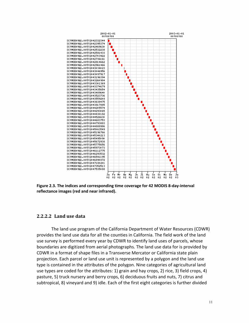
Two MODIS Terra image sets are used in this study: 16-day-interval vegetation index (Normalized Difference Vegetation Index, NDVI and Enhanced Vegetation Index, EVI) at 250 m spatial resolution and 8-day-interval surface reflectance at 250 m spatial resolution for red (620-670 nm) and near infrared (841-876 nm) bands. The origin images in sinusoidal projection have the geographic center at 35.34° Lat, -116.34° Lon, and the geographic extent is defined by the four corner points: 29.83° Lat, - 115.37° Lon; 40.00° Lat, -130.54° Lon; 40.09° Lat, -117.36° Lon; 29.91° Lat, -103.70° Lon. The images are obtained at no cost from NASA’s Earth Observation System Warehouse Inventory Search Tool (discontinued, updated data sources are at https://lpdaac.usgs.gov/), where the images are corrected for the effects of atmosphere, dynamic aerosol and cirrus clouds. The quality is ensured, and for most cloud and snow free, low aerosol load pixels, the values are very reliable. However, MODIS was off during a 15-day period, leaving a data gap in June, 2002. In total 19 NDVI images and 42 reflectance images are used. The time coverage of vegetation index and Reflectance are illustrated in Figure 2.2 and Figure 2.3, respectively.

Figure 2.2. The indices and corresponding time coverage for 19 MODIS 16-day-interval vegetation index images, which include the bands NDVI.

11

Figure 2.3. The indices and corresponding time coverage for 42 MODIS 8-day-interval reflectance images (red and near infrared).

2.2.2.2 Land use data

The land use program of the California Department of Water Resources (CDWR) provides the land use data for all the counties in California. The field work of the land use survey is performed every year by CDWR to identify land uses of parcels, whose boundaries are digitized from aerial photographs. The land use data for is provided by CDWR in a format of shape files in a Transverse Mercator or California state plain projection. Each parcel or land use unit is represented by a polygon and the land use type is contained in the attributes of the polygon. Nine categories of agricultural land use types are coded for the attributes: 1) grain and hay crops, 2) rice, 3) field crops, 4) pasture, 5) truck nursery and berry crops, 6) deciduous fruits and nuts, 7) citrus and subtropical, 8) vineyard and 9) idle. Each of the first eight categories is further divided

12

into individual plant types, which are used as the ground truth data in this study. Most of the parcels are single-use during the year while others are multiple cropping types.

In this study the counties of interests and the corresponding survey years are: Kings (1991, 1996 and 2003), Fresno (1984, 1994 and 2000), Merced (2002) and Sutter (1998 and 2004). Multi-temporal land use maps are used for Kings, Fresno and Sutter to detect land use change, and the land use of Merced is examined in detail and processed to perform classification. The study focuses on the agricultural land use in year 2002, when the latest survey in Merced County was performed. More than sixty types of polygons are extracted from the shape file, and nine types whose combined polygon acreages are greater than 10,000 are considered as major types. Table 2.1 shows that these nine major types comprise 83% of the distinguishable agricultural lands.

Table 2.1. Major agricultural types determined from land use survey in Merced County, 2002

Name Acreage Percent Almonds 96439 17% Alfalfa & alfalfa mixtures a 91143 17% Grain <-> Corn b 66576 12% Cotton 59781 11% Mixed pasture 44235 8% Grain and hay crops c 36871 7% Tomatoes 29998 5% Corn (field & sweet) d 16311 3% Vineyards 14260 3% Others 90631 17% Total 546246 100% a: “Alfalfa” for short. b: A rotational type with grain and corn grown alternately. c: Includes wheat, barley, and oats. “Grain” for short. d: “Corn” for short.

2.2.3 Change detection

The method to detect agricultural land use change between different years’ survey data is based on the spatial intersection performed by ESRI ArcGIS. First all the agricultural land parcels are extracted and the total area is calculated. The parcels change from agricultural land to non-agricultural land or vice versa are also counted in. Parcels with identical values for the attributes of different years are considered as “no change” parcels, while others are changed parcels. The agricultural land use change ratio is defined as the area of changed parcels over the total agricultural land area (Table 2.2).

13

2.2.4 Classification

The classification processes focus on the nine major crop types defined in Table 2.1. First, the 19 MODIS NDVI images through the year 2002 are used to perform the classification, with a time interval of approximate 16 days. To derive the “ground truths” points from the survey shape file, a buffer with a negative distance (-100 m) is created first to eliminate the influences of the mixed pixels along the parcel boundaries, and those buffered areas are converted into raster format with the type codes as point values. The number of ground truth points for each crop varies from 76 to as many as 500. The average NDVI values are calculated for each crop class, and those values are plotted versus the order number of NDVI images to analyze their separability. Then a maximum likelihood algorithm is used for the classification with a probability threshold set to 0.5. 50% of those ground truth points are extracted randomly as the training set, and the other 50% of points form a test set. This procedure repeats ten times, and the mean and the standard deviation of the ten classifications are calculated. Of practical concern is how early in the year the agricultural land use of the whole year can be identified. Therefore in the next step, the number of NDVI images used is changed to n (n≤19), and only the images from the 1st to the nth comprise the input bands for the maximum likelihood classification. One of the training sets generated above is used for training and the validation process is performed using the corresponding test set. Since the 250 m resolution NDVI images are actually produced from the 250 m resolution MODIS surface reflectance for red and near infrared, the original reflectance images at a time interval of 8 days are then used to perform the classification. The time interval for NDVI images is two times as long as the time interval for surface reflectance images, and each reflectance image has two bands (red and NIR), so for each NDVI image there are four corresponding reflectance bands and with more available information the distinguishing power is likely to be improved. The same classification method and training and test sets are used as the previous steps.

2.3 Results

For the counties with multi-year land use data available, the land change ratio is calculated for each time period and shown in Table 2.2.

Table 2.2. Land use change during periods between survey years.

County name Periods Changed acreage Total acreage Change ratio (%) Kings 1991-1996 394883 591238 66.79

1996-2003 375681 577953 65.00 Fresno 1986-1994 1004809 1347669 74.60

1994-2000 961184 1337723 71.85 Sutter 1998-2004 123889 298984 41.44

14

The plot of NDVI values versus the order number of the image reflects the seasonal trends for the crop classes (Figure 2.4). The classification with 19 NDVI images repeats 10 times using a different random partition of the ground truth points as training sets and test sets, and the result is given by Table 2.3. The confusion matrices of the classifications are quite similar, and the confusion matrix with producers’ and users’ accuracy for the first pair of training and test set is given in Table 2.4.

Figure 2.4. Seasonal trends of NDVI values for major crop classes by day of year (DOY) within the time coverage of the 19 NDVI images.

Table 2.3. Overall accuracy and kappa coefficient for classification using the whole NDVI series.

No. of Test Overall accuracy (%) Kappa Coefficient 1 80.3406 0.7715 2 81.7035 0.7870 3 81.9584 0.7900 4 81.7300 0.7870 5 81.6788 0.7870 6 80.4124 0.7725 7 81.2995 0.7825 8 80.7018 0.7761 9 80.5732 0.7748

10 80.2362 0.7695 Mean 81.0634 0.7798

Standard Deviation 0.6742 0.0077

15

Table 2.4. Confusion matrix for one of the classifications using 19 NDVI images.

Class Ground truth

Total Users’ Accu. (%) 1 2 3 4 5 6 7 8 9

Unclassified 1 3 6 9 4 7 2 32 Almonds(1) 157 7 2 9 3 178 88.2 Cotton(2) 102 1 1 8 2 114 89.4 Corn(3) 2 6 14 2 1 3 28 50.0 Grain(4) 2 179 11 2 13 207 86.4 Grain<->corn(5) 4 2 6 121 5 3 2 143 84.6 Alfalfa(6) 3 8 5 3 7 247 13 4 290 85.1 Mixed pasture(7) 7 8 3 5 139 4 166 83.7 Tomatoes(8) 4 13 12 6 5 2 1 45 88 51.1 Vineyards(9) 6 1 2 3 34 46 73.9 Total 182 136 40 219 152 274 181 62 46 1292 Prod’s accu. (%) 86.2 75.0 35.0 81.7 79.6 90.1 76.8 72.5 73.9 In the classification, if only the first nth NDVI images are used, then the accuracy and kappa coefficient increase with the number of images used. This relationship is shown in Figure 2.5 for the first pair of training set and test set. If the 8-day-interval surface reflectance images are used instead of the NDVI images, the accuracy and kappa coefficient also increase with the number of images used but at different rates (Figure 2.6). Two surface reflectance images correspond to one NDVI image during the same period. Though 42 images from the beginning of 2002 are available, there are not enough ground truth points for some types and the classification cannot be performed if the total number of bands exceeds 35, so the maximum number of images used is 17 (17<35/2).

16

(a)

(b)

Figure 2.5. Plots of accuracy (a) and kappa coefficient (b) versus the number of NDVI images used in classification.

0

10

20

30

40

50

60

70

80

90

3 4 5 6 7 8 9 10 11 12 13 14 15 16 17 18 19

Accu

racy

(%)

Number

0

0.1

0.2

0.3

0.4

0.5

0.6

0.7

0.8

0.9

3 4 5 6 7 8 9 10 11 12 13 14 15 16 17 18 19

Kapp

a Co

effic

ient

Number

17

(a)

(b)

Figure 2.6. Plots of accuracy (a) and kappa coefficient (b) versus the number of surface reflectance images used in classification.

0

10

20

30

40

50

60

70

80

6 7 8 9 10 11 12 13 14 15 16 17

Accu

racy

(%)

Number

0

0.1

0.2

0.3

0.4

0.5

0.6

0.7

0.8

6 7 8 9 10 11 12 13 14 15 16 17

Kapp

a Co

effic

ient

Number

18

2.4 Discussion

In the land use change detection (Table 2.2) it is observed that for the counties Kings and Fresno, Over 60% of the agricultural lands have changes in plant type during the less-than-ten-year time intervals. For Sutter, which is a major producing area for rice, the change ratio is not so high, but still over forty percent. The changes in agricultural land use from year to year are mostly determined by the market factors, and the variance is especially high for economic agricultural plants. Therefore, the lands in those important agricultural counties generally have considerable changes, and it is necessary to develop an efficient and effective way to do the up-to-date survey rather than relying on the former land use map.

The classification using NDVI image series all through the year 2002 demonstrates a high distinguishing power since generally the agricultural plants show different seasonal trends for NDVI values (Figure 2.4). However, the low accuracies for some classes are not acceptable in application. Neither the user’s accuracy nor the producer’s accuracy for the type “corn” are more than 50% and the users’ accuracy “tomatoes” is only 51.1% (Table 2.4). From the confusion matrix it is found that a large proportion of “corn” pixels are classified as “tomatoes” and “cotton” pixels are classified as “corn”. There are two reasons for the low accuracies: i) some plant classes have similar seasonal trends in NDVI values, and ii) the plant classes with low accuracies have relatively small total areas and also small parcel sizes, so the numbers of available “pure” pixels for those classes are limited and thus the composition of the training set is biased. Therefore, to improve the overall classification accuracy, on one side more detailed knowledge on the seasonal trends of crops should be gained, and on the other finer spatial resolution data than the 250 m MODIS images is necessary which requires more processing time.

In the classification using NDVI series, at least 12 consequent NDVI images are needed to increase the accuracy to approximately 75% (Figure 2.5). The surface reflectance images provide more spectral information about the plants’ seasonal trends, and only 17 reflectance images, which correspond to less than 9 16-day-interval NDVI images, are needed to produce the same level of overall classification accuracy (Figure 2.6). Such number of reflectance images can be acquired as early as the beginning of May of the year, which means that the mapping of the agricultural land use of the whole year can be accomplished at an early time and the land use information can be employed in the agricultural management such as water resource allocation for the remaining of the year.

2.5 Summary

The large change ratios in the agricultural land use in several important agricultural counties in California show the necessity of an effective and efficient mapping approach. However, the medium spatial resolution limits the availability of the pure ground truth pixels and reduces the accuracy of the classification focusing on the

19

major agricultural plant types. With higher spatial resolution, the effect of mixed pixels is likely to be reduced and thus the classification can be improved. The NDVI image series all through a year demonstrate the power to identify the seasonal trends and distinguish the agricultural plants, and the surface reflectance images, which are the source of the NDVI, provide more bands to delineate the seasonal trends. Using surface reflectance images, it is possible to map the major agricultural plant types of the year almost as early as in the first four months, and such a timely agricultural land use map can surely help the agricultural management for the remaining of the year. The shortcomings of the classification approach in this study are apparent. Due to the parametric characteristic of the maximum likelihood classifier, high accuracies achieved in this study highly depend on a large and reliable training set. The size of the training set for each crop type should be at least greater than the number of bands used in the classification (so classification using surface reflectance images requires a larger ground truth dataset than using NDVI images). In practice, a much larger size than the ideal minimum is required to fully represent the distribution in a multi-dimensional space. However, for most years without land use surveys such a large set of high quality ground truth points is unavailable. Ground truths collected in one year cannot be used directly in the training of another year's classification because growing seasons of crops are variable as a result of changing weather and markets. The shortage of ground truth data for training is the most limiting factor of crop mapping using a traditional MLC approach.

20

Chapter 3. Phenology based classification of major crop types in the San Joaquin Valley, California

3.1 Background

Existing classifiers are not able to effectively map crop types in the Central Valley with shortcomings discussed in Chapter 2 as a result of complicated environmental conditions and diverse agricultural systems. A variety of techniques including curve-fitting, decision tree, and object based classification are explored to develop a phenology based classification (PBC) approach for the purpose of crop mapping. Introductions to these techniques and motivations of classifier development have been given in Chapter 1.

3.2 Materials and methods

3.2.1 Study area

This study was carried out in the San Joaquin Valley (SJV), the south part of the Central Valley (Figure 3.1). This area is characterized by vast flat terrain, high agricultural productivity and Mediterranean climate with hot dry summers and cool rainy winters. Two counties were the focus of our study: Merced County (ME) in the northern part of SJV and Kern County (KN) in the south end. Both of the counties are of great importance in agriculture. According to the latest agricultural statistics database in the year 2007 (USDA, 2009), KN and ME had the 1st and 5th largest total farmland acreage in California, respectively. The annual average precipitation of ME is below 380 mm, and KN below 250 mm. Agriculture in both counties relies heavily on irrigation.

21

Figure 3.1. The San Joaquin Valley and the two counties of special interest shown on California topographic map.

3.2.2 Data

3.2.2.1 MODIS 250 m reflectance (MOD09Q1) data

MODIS red and near infrared reflectance 8-day composite images at 250 m spatial resolution (MOD09Q1 product) are obtained from NASA’s Earth Observation System Warehouse Inventory Search Tool (discontinued, updated data sources are at https://lpdaac.usgs.gov/), where the images have been corrected for the effects of atmosphere, dynamic aerosol and cirrus clouds. A quality assessment flag is provided

22

within MOD09Q1 to evaluate the data quality of each pixel. The entire SJV is covered by one scene of MOD09Q1 image, which is row 05 and path 08 (h08v05). All available images in year 2002, 2006, 2007 and 2008 are acquired and reprojected to Albers equal-area conic projection using MODIS Reprojection Tool (MRT, https://lpdaac.usgs.gov/lpdaac/tools/modis_reprojection_tool).

3.2.2.2 CDWR land use data

The land use survey of the California Department of Water Resources (CDWR) provides the most reliable land use data for all counties in California. Crop survey is taken every year by CDWR for counties alternately, at a frequency of every 5-10 years for an individual county. Each parcel or land use unit is digitized from an aerial photograph as a polygon and assigned a label of crop type. Details of the land use program and data are given in Section 2.2.2.2. Though the land use data is of high quality, the acquisition is labor intensive and expensive. Furthermore, timely information may not be available for management because the survey frequency is too low to detect agricultural land use changes and considerable time is needed to finish each survey and process the data. The latest survey in ME was performed in year 2002. More than sixty crop types of polygons were found from the crop survey data. Eight specific types whose total areas were greater than 4,000 ha were considered as major crop types. These major crop types comprised 75% of the total size of crop lands (Table 2.1). The average field size was ~15 ha, and ~80% of the fields were smaller than 20 ha, corresponding to less than four MODIS 250 m pixels. Compared to ME, KN has greater diversity in crop types and larger field sizes. According to the surveyed land use map of KN in year 2006, twelve specific types were considered as major crop types. These crop types comprised ~85% of the total size of crop lands (Table 3.1). The average field size was ~28 ha, and ~80% of the fields were smaller than 40 ha, corresponding to less than seven MODIS 250 m pixels.

23

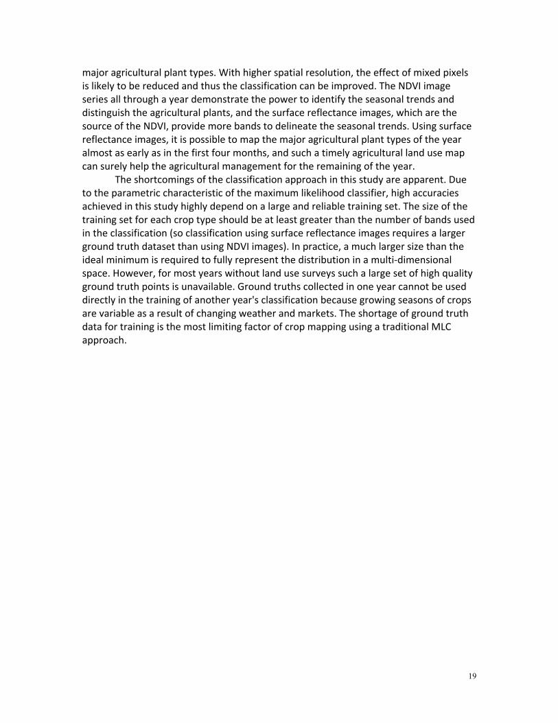
Table 3.1. Major crop types of KN from land use survey in year 2006.

Type Total area (ha) Percentage of agricultural land use

Almonds 69207 18.9 Vineyards 41859 11.4 Cotton 41818 11.4 Grain 37803 10.3 Alfalfa 36691 10.0 Pistachios 25526 7.0 Oranges 22237 6.1 Carrots 10038 2.7 Grain & corn 9494 2.6 Corn 9271 2.5 Onions & Garlic 4468 1.2 Tomatoes 3989 1.1 Unspecified 26694 7.3 Others 27713 7.6 Total 366814

3.2.2.3 USDA CDL

The USDA Crop Data Layer (CDL) in year 2007 includes a crop-specific land cover map for the entire state of California. There are two versions of 2007 California CDL, one derived from 56 m AWiFS (Advanced Wide Field Sensor) satellite imagery and the other from 30 m Landsat 5 TM imagery, and the latter was used for its finer spatial resolution and higher reported accuracy. The CDL was produced based on the supervised classification of TM imagery. There was a variety of ancillary datasets used in the classification including the United States Geological Survey (USGS) National Elevation Dataset (NED), the USGS National Land Cover Dataset 2001 (NLCD 2001), and MODIS 250 m 16 day NDVI composites. A total of 36 specific crop classes and 9 non-agricultural classes are presented for the entire state of California. The classification accuracy was as high as 97.22% according to the metadata provided by USDA NASS. However, the accuracy is likely to be over-estimated as a result of over-fitting and other factors based on visual assessment. Efforts are not made specifically to determine the major crop types of the entire SJV because CDL is not a completely reliable crop type map and the classification scheme of CDL is different from the scheme of this study. The major crop types of ME and KN are still used as classes of interest based on the assumption that these major crop types could represent most of the cropland cover in the study area. The selected set of interested crop types in the CDL is utilized as ground truth reference data for validation. There is no strict one-to-one relation between the classes in the CDL and the crop types focused by this study, so some modifications were made on the classes. The

24

rotation type grain & corn and the single use type corn are not distinguished in the CDL, so the corresponding types in the classified image are merged to facilitate validation. In the CDL pistachios were not explicitly identified but combined with other classes to form a miscellaneous type “other tree nuts & fruits”, so classification of pistachios is not validated using the CDL.

3.2.2.4 Field data

I conducted cropland field sampling in KN in year 2008. Sample fields were visited multiple times to capture the crop types in various seasons. Generally the recognized fields distributed evenly across the entire county, and all crop types were recorded. Pixels in MODIS images in 2008 corresponding to the fields were labeled with the crop types and used for accuracy assessment. No matter how large the field was, it was represented by only one point. If a field is small it was not sampled to make sure that points recorded by the GPS unit locate at pure pixels in the remotely sensed images.

3.2.3 Method

3.2.3.1 MODIS time series preprocessing

In this study, the MOD09Q1 products are utilized to derive “phenological metrics”, and a classifier is developed to work on these phenological metrics to identify specific crop types. This is the major difference from traditional multi-temporal classification algorithms, which focus on the distribution of original remotely sensed variables (surface reflectance or vegetation indices) rather than derived metrics associated with phenology. Red and infrared bands are extracted from all available MOD09Q1 products within each study period. For a certain year, since winter grain is usually sowed at the end of the last year, the beginning of the study period is extended to November of the last year. The end of the study period is the end of the calendar year or the first one or two weeks of the next year, if no images are available at the year end. All the 250 m 8-day surface reflectance images within each study period were applied with Equation (2) and sequentially stacked to generate NDVI profiles:

rednir

rednir

BBBB

NDVI+−

= (2)

where Bnir and Bred are surface reflectance for the near infrared and red bands respectively. Less reliable data is removed based on the quality flag and replaced by temporal linear interpolation. Because the curve-fitting approach used in this study (Section 3.2.3.2) tends to be affected by false low or high NDVI values (Pettorelli et al., 2005), NDVI profiles are smoothed first. An iterative smoothing algorithm is performed for the NDVI profile of every pixel: in each iteration the deviation of each NDVI value from the two neighbor values is calculated and the value with maximum deviation is

25

replaced with the mean of neighbor values, until the maximum is smaller than a threshold.

3.2.3.2 Derivation of phenological metrics

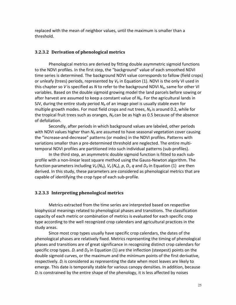
Phenological metrics are derived by fitting double asymmetric sigmoid functions to the NDVI profiles. In the first step, the “background” value of each smoothed NDVI time series is determined. The background NDVI value corresponds to fallow (field crops) or unleafy (trees) periods, represented by Vb in Equation (1). NDVI is the only VI used in this chapter so V is specified as N to refer to the background NDVI Nb, same for other VI variables. Based on the double sigmoid growing model the land parcels before sowing or after harvest are assumed to keep a constant value of Nb. For the agricultural lands in SJV, during the entire study period Nb of an image pixel is usually stable even for multiple growth modes. For most field crops and nut trees, Nb is around 0.2, while for the tropical fruit trees such as oranges, Nb can be as high as 0.5 because of the absence of defoliation. Secondly, after periods in which background values are labeled, other periods with NDVI values higher than Nb are assumed to have seasonal vegetation cover causing the “increase-and-decrease” patterns (or modes) in the NDVI profiles. Patterns with variations smaller than a pre-determined threshold are neglected. The entire multi-temporal NDVI profiles are partitioned into such individual patterns (sub-profiles). In the third step, an asymmetric double sigmoid function is fitted to each sub-profile with a non-linear least square method using the Gauss-Newton algorithm. The function parameters including Vb (Nb), Va (Na), p, Di, q and Dd in Equation (1) are then derived. In this study, these parameters are considered as phenological metrics that are capable of identifying the crop type of each sub-profile.

3.2.3.3 Interpreting phenological metrics

Metrics extracted from the time series are interpreted based on respective biophysical meanings related to phenological phases and transitions. The classification capacity of each metric or combination of metrics is evaluated for each specific crop type according to the well recognized crop calendars and agricultural practices in the study areas. Since most crop types usually have specific crop calendars, the dates of the phenological phases are relatively fixed. Metrics representing the timing of phenological phases and transitions are of great significance in recognizing distinct crop calendars for specific crop types. Di and Dd in Equation (1) are the inflection (steepest) points on the double sigmoid curves, or the maximum and the minimum points of the first derivative, respectively. Di is considered as representing the date when most leaves are likely to emerge. This date is temporally stable for various canopy densities. In addition, because Di is constrained by the entire shape of the phenology, it is less affected by noises

26

(Fisher & Mustard, 2007). Similarly, Dd is the date with the most rapid decrease of leaf content. Generally Dd has the same advantages as Di, especially for field crops that are cultivated in a short time. Comparatively, Dd is more uncertain for trees because defoliation is gradual and the rate depends on weather conditions and water availability. Thus, Di and Dd are important phenological metrics used to distinguish crops with different crop calendars. Among other metrics in Equation (1) derived from curve-fitting, p and q are also useful in classification since crops show different NDVI increasing and decreasing rates in green-up and defoliation (or harvest) stages. Nb and Na also have the potentials to classify crops with different NDVI levels. However, NDVI is sensitive to crop density and may show large variation within each crop type, so the relationship between crop type and NDVI values at certain stages is inconsistent. Besides the fitting parameters above, some useful metrics are not explicitly given by Equation (1). For annual NDVI profiles with multiple modes, some crop types could be implied by the number of modes (n). For example, crop rotation between wheat and corn usually has n=2. Another example is alfalfa, a major pasture in the study areas which is characterized by multiple same-year planting/cultivation and short growing seasons (~2.5 months). The sowing dates are highly uncertain, distributing randomly within most of a year. Curve-fitting is not effective as a result of the short growing periods. While metrics derived from curve-fitting are not available, the value of n greater than 4 or 5 become a reliable criterion to identify alfalfa. Crops with stable crop calendars tend to maintain a high level of NDVI for a certain period within the growing season. The difference (Dd - Di), which is the length of high NDVI period (LHNP), is a good indicator of the length of growing season of different crops. LHNP is of great importance in recognizing crops with distinct lengths of growing season, for example, cotton and tomatoes. While the DOYs with the most rapid changes of NDVI could be found by inspecting the first derivative of the curve, higher order derivatives of NDVI profile also have the potential of representing phenological phases (Soudani et al., 2008). In this study, the DOYs when the second derivative of the NDVI profile reached extrema are focused. Among the four such DOYs of a double sigmoid function, the first point, D1, is selected as an indicator of the onset of greenness and the fourth point, D4, is selected as an indicator of the onset of dormancy/fallow (Figure 1.1). The expressions of D1 and D4 are given by:

226ln1

226ln1

4

1

−−=

−+=

pDD

pDD

d

i

(3)

All terms are defined previously. This approach is slightly different from previous studies, where the extrema of curvature was used instead of the extrema of the second derivative (Zhang et al., 2003). The time between D1 and D4, (D4-D1), is defined as the length of the growing season (LGS). These metrics are used in crop mapping when they have higher accuracy in characterizing crop growth than Di, Dd and LHNP.

27

3.2.3.4 Decision tree classifier

Decision trees predict class membership by recursively partitioning a dataset into more homogeneous subdivisions (De Fries et al., 1998). The decision tree classifier has substantial advantages for remote sensing classification because of its flexibility, intuitive simplicity, and computational efficiency (Thenkabail et al., 2009, Friedl & Brodley, 1997). In particular, the decision tree classifier is a nonparametric classifier which makes no assumptions concerning the statistical distributions of the input variables. Decision tree classifiers with phenological metrics as input data are suitable in mapping crop types, because mathematically predefined distributions of phenological metrics could rarely be found for crop types. For example, sowing date is selected based on variety and human decision, which are difficult to be modeled by parametric distributions. The assumption of central tendency employed by many traditional classifiers tends to fail in agricultural systems. In addition, the great flexibility of decision tree classifiers guarantees that they could easily adjust to new local conditions and crop types by modifying a part of the decision tree. Thresholds of a decision tree classifier are determined based on crop calendars, knowledge on agricultural practices, and visual interpretation of MODIS NDVI profiles. A constructed decision tree was applied to phenological metrics of the pixels within SJV in year 2002, 2006, 2007 and 2008. The same decision tree is applied to all the study years since no extreme meteorological and artificial conditions are observed among these years. One problem of this approach is that the accuracy assessment tends to be slightly biased because the entire ground truth dataset was used as the test set, but a part of the ground truth dataset is already used to interpret NDVI seasonal profiles of each crop type. However, this effect is trivial because only a very small number of parcels (<10 for each type) are used in the process of decision tree construction. All the crop types are divided into three categories and each category is treated individually by the decision trees. The first category consists of crops such as grain (including wheat, barley and oats), corn, cotton and tomatoes, whose increasing and decreasing NDVI trends in NDVI profiles are closely related to agricultural practices such as sowing and harvest. The crop cover is assumed to be completely removed after harvest. The second category includes nut trees (almonds and pistachios) and vineyards, whose NDVI variations are caused by phenological phase transitions such as green-up, senescence and defoliation. These two categories are considered as having “normal” NDVI profiles within a growing season. Other crop types that do not have normal NDVI profiles belong to the third category, including alfalfa and oranges. Alfalfa has flexible planting dates and multiple short growing seasons (~2.5 months) that cannot be fitted properly by the double sigmoid function. Oranges maintain a high (>0.4) and semi-constant level of NDVI values as a result of subtropical plant characteristics. The NDVI profiles of oranges cannot be fitted by the double sigmoid function, but oranges can still be easily recognized by their high Nb and low Na values. Crop types in the third category are handled individually in special ways by the decision tree.

28

3.2.3.5 Validation

The crop classification map derived from remote sensing is validated using reference data in the study areas (land use polygons for ME 2002 and KN 2006, CDL for the entire SJV 2007, and field survey data for KN 2008). For ME 2002 and KN 2006, ground truth data of each entire county are available from the DWR land survey polygons so the test dataset included all the crop parcels in these counties. Pixel-based validation is performed rather than parcel-based method because i) parcel edges could not be precisely extracted from the MODIS data due to the relatively small parcel size and relatively coarse resolution, ii) locations of parcel edges could not be precisely determined in field survey, and iii) in the pixel-based validation large parcels gain more weight so the result is not biased by the many parcels that are smaller in size than the 250 m footprint of the MODIS data in the study areas. In addition, if equal-area projection is used (as the case of this study), the number of correctly classified pixels represents the total area of the croplands that are successfully identified. The test set for 2007 is derived from the preprocessed CDL. Within each 250 m MODIS pixel, 30 m CDL grids for each crop type are counted and the majority type is treated as the ground truth of the corresponding MODIS pixel. The majority type must exceed 50% of the land cover within each MODIS pixel or the pixel is labeled as unclassified at the MODIS resolution and eliminated from validation. In total 143772 250 m ground truth points are generated for SJV in 2007 using the CDL. For KN 2008, accuracy assessment is only performed using the field sample data because the limited coverage of fieldwork. Confusion matrices are created for the four crop maps in the respective study areas.

3.2.3.6 Maximum likelihood classification

For the sake of comparison, the traditional MLC is also applied to the three land survey datasets: ME 2002, KN 2006, and KN 2008. The CDL in 2007 is excluded because the reliability of this resampled product is relatively low for the retrieval of suitable training datasets and the difference in classification scheme prevents its use in producing a map of desired crop types. For the two datasets of ME 2002 and KN 2006, the ground truth reference data from land use survey data are split into training sets and test sets. Because the PBC approach requires a very small training set as one of its main advantages, attention is paid to the performance of the MLC with various sizes of training sets. In this study, ground truth datasets used in the MLC are split randomly with 3 different ratios: 10:90 (10 percent as the training set and 90 percent as the test set), 20:80 and 50:50 as long as the minimum requirements on the size of the training set are met. Training and validation are performed for each split group respectively. Unlike ME 2002 and KN 2006, KN field data in 2008 is used entirely as the test set. The trained parameters from KN 2006 are directly used in the MLC of the images in 2008. The reasons for the different treatment are: i) the comparison aims to test the stability

29

of the maximum likelihood classifier in multi-year classification which is affected by inter-annual variation, and ii) the relatively small size of the field data in 2008 does not suffice the minimum requirements on the size of the training set after the splitting process. Confusion matrices are generated for the accuracy assessment.

3.3 Results

3.3.1 Decision tree building

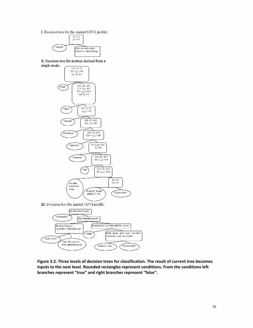
A decision tree is constructed mainly based on local crop calendars with derived phenological metrics as input variables. The final decision tree is designed in a hierarchical manner. Firstly, oranges are extracted by examining the annual NDVI profiles, which show semi-constant high NDVI level throughout the year. Since annual NDVI profiles of oranges include no increasing-and-decreasing growing modes, time related metrics are not derived from curve-fitting by the double sigmoid function and thus Nb and Na become the sole criteria to identify orange pixels. Secondly, NDVI profiles that are not recognized as oranges are split into individual growing modes. Each growing mode is classified by a new decision tree (Figure 3.2, II) to identify the specific crop type of the mode. Thirdly, the type of the entire annual NDVI profile is determined based on the identified individual modes within the profile. If there is no identified mode, the pixel is labeled as “unclassified”. If there is only one identified mode, the pixel is labeled with the crop type of the mode. For profiles with more than one identified modes, two multiple-use crop types are considered specifically: alfalfa and the rotation type “grain & corn”. Alfalfa is a pasture type with multiple cuts at short intervals. Annual NDVI profiles with 4 or more qualified short modes are recognized as alfalfa. Another major crop type, grain & corn, refers to winter grain and summer corn planted alternately in the same year and parcel. NDVI profiles containing both the two identified types are labeled as this rotational type. Since the planting of corn in this rotational type tends to be delayed compared to fields with only corn planted in a year, the NDVI peak in late summer is identified as corn only when grain is identified earlier in the current year. The three steps are completed by three decision trees, given in Figure 3.2. Usage of metrics for individual crop types is further discussed in the following sections.

30

Figure 3.2. Three levels of decision trees for classification. The result of current tree becomes inputs to the next level. Rounded rectangles represent conditions. From the conditions left branches represent “true” and right branches represent “false”.

31

3.3.1.1 Nut trees & vineyards

The three types, almonds, pistachios and vineyards, have regular annual NDVI profiles, whose NDVI begin increasing as a result of green-up in spring, maintain a high level throughout the summer, decrease gradually following the late fall defoliation and have a low value in winter before budburst. NDVI profiles are less influenced by human practices, and mostly depend on climate and regional factors that are relatively stable. Di is the most important parameter to distinguish nut trees and vineyards from other crop types. Those summer field crops (cotton, corn and tomatoes) may have similar Di values to pistachios and vineyards, but pistachios and vineyards usually have a longer green period with high NDVI level. In this case, LHNP becomes a useful parameter showing phenological distinction of pistachios and vineyards from other crop types. For the classification between these three types, Di of almonds is ~80 and Di of pistachios and vineyards is ~120, so almonds are distinguished very well by Di. Classification between pistachios and vineyards is more challenging and only using Di is inadequate. From observations, LHNP of pistachios is slightly longer than that of vineyards. Furthermore, for pistachios the decrease of NDVI in late fall is not as gradual as vineyards, so the type of pistachios has bigger values of parameter q. The uses of LHNP and q partly solved the problem of confusion between pistachios and vineyards.

3.3.1.2 Grain

Grain (including wheat, barley and oats) is the only early season (winter) crop in major crop types. The distinct crop calendar is adequate to separate grain from other major crop types. By visual examination, Di is between ~ -20 and ~80, and LHNP is between ~50 and ~120. Usually larger Di is associated with shorter LHNP. Grain can also be planted for green chop to feed livestock, which is harvested early before the mature phase. Thus it is also possible for the type of grain to have short LHNP. Though grain has distinct Di values and certain LHNP ranges, confusion occurs between grain and weeds, which grows in the same season as grain when rainfall is sufficient. Weeds growing in fallow parcels are separated effectively from grain when the NDVI level is equivalent.

3.3.1.3 Summer field crops

Summer field crops (cotton, corn and tomatoes) have similar crop calendars. Summer field crops are easily identified with fixed growing seasons, but are further divided into specific types with high confusion rates. Di and LHNP ranges of cotton, corn and tomatoes are only slightly different and have great overlap, increasing the difficulty of classification. The type grain & corn refers to a rotation between early season grain (mostly wheat) and late season corn as stated above. Rotations between grain and other summer crops are very rare in our study areas. So when grain and an unspecific summer

32

crop type are both found in the annual NDVI profile, the summer crop type is most likely to be corn and the pixel with such a double-peak NDVI profile is classified as “grain & corn”.

3.3.1.4 Oranges

With subtropical nature, oranges maintain a high NDVI level all year long. NDVI variation of this type cannot be modeled by the double sigmoid function (repeat as before). High Nb (>0.40) and low Na (<0.20) are sufficient criteria to classify oranges from other major types. When summer water depression occurs, NDVI of oranges may drop slightly so the annual NDVI profile shows a “U” shape. Too low summer NDVI is one possible reason for under-classifying oranges, but this case is rare. The biggest confusion associated with the crop type oranges is that natural forests in adjacent mountainous areas are sometimes misclassified as oranges. Those forests are generally far away from crop land so the misclassified pixels are easily masked out in post-processing.

3.3.1.5 Alfalfa

Multiple short growing cycles in a year distinctly characterize the planting and harvest pattern of alfalfa. NDVI variation within each cycle is not modeled by a double sigmoid function since the growing period is too short and only a limited number of observations are available for each period. In addition, flexible dates for planting and harvest make the parameters Di and Dd useless in classification. Each growing cycle is identified as alfalfa by 1) the length of the entire cycle, represented by LGS, which should be shorter than 64 days (eight 8-day periods), and 2) the difference between the maximum and minimum NDVI within the cycle, which must be greater than 0.3. Pixels with more than 4 such recognized cycles in a year are considered as alfalfa fields. Alfalfa is the dominant pasture type in our study areas. Many parcels are intercropped with alfalfa and other pasture types. The total area of such “mixed pasture” parcels is considerable, but the land use of these parcels is regarded as a nonspecific type and excluded from the assessment dataset. Since alfalfa contributes to the NDVI variation of the mixed pasture fields, many of the pixels in those fields are classified as alfalfa, which is reasonable but is not validated by field data. For this reason, the actual classification accuracy for alfalfa is not exactly represented by the accuracy assessment.

3.3.1.6 Other major crop types

All the major crop types of ME have been discussed above and the corresponding decision tree thresholds are determined accordingly. However, in KN, two major types, carrots and onions & garlic (onions and garlic have similar characteristics and belong to the same type in the land use survey data), cannot be

33

classified using phenological metrics. Both of the two types have relatively flexible crop calendars, multiple growing cycles and short growing periods, which is similar to alfalfa and alfalfa intercropping pasture. However, compared to alfalfa, these two types have more irregular NDVI profiles, which are very difficult to recognize from phenological metrics. Thus the PBC approach is not designed to deal with the crop types of carrots and onions & garlic.

3.3.2 ME 2002 crop mapping

Classification of specific types is challenging in ME, where crop land parcels are usually small and patchy (~4 MODIS 250 m pixels on average). Identified crop types that are major types of KN (Table 3.1), but not major types of ME (Table 2.1) are treated as unclassified. By visual assessment, classified crop patterns are generally in agreement with the surveyed crop patterns (Figure 3.3). Summer crops and alfalfa in the southwest part of ME, almonds and vineyards in the northeast, and rotation cropping areas of grain and corn in the north are well depicted. Center pixels of large parcels are recognized very well, while most of the pixels along parcel edges are unclassified. As a result, parcels in the classification map are usually smaller than the corresponding parcels in the survey map, and some parcels are not identified when they only occupied several mixed pixels on the images. The confusion matrix shows that the specific crop type map of ME has an overall accuracy of 70.0%. Though this accuracy is not high, according to the first row of the confusion matrix, the major source of error is too many unclassified pixels. By observation it is found that the edge effect described above is the major reason for this kind of confusion. Excluding the first row, the remaining confusion matrix has an accuracy of 82.9%, showing that for the classified pixels the chance of correct identification is high. Therefore, such level of accuracy already has great potential in specific crop type mapping, especially when parcel edges can be acquired from other data sources as auxiliary data. The accuracy by the MLC method varies significantly with the splitting percentages. In the 50:50 group (50% of ground truth reference data are used as training data) high accuracy (80.1 %) is achieved, which is consistent with the accuracy reported for ME in a previous paper (Zhong et al., 2009). The 50% large training set made the MLC more accurate than the PBC approach. In addition, unlike the PBC approach, the MLC generates only a few unclassified pixels as a result of a low probability threshold and most of the confusion exists between classes. However, as the size of the training set decreases the accuracy of the MLC drops significantly. The accuracy is 75.6% for the 20:80 group, and only 66.8% for the 10:90 group. So when the training set is smaller than 10% of the entire coverage, the MLC fails to yield acceptable results.

34

Figure 3.3. (a) Phenology-based crop classification map from MODIS NDVI time series versus (b) DWR survey map as the reference data, for ME 2002.

3.3.3 KN 2006 crop mapping

KN has slightly larger average parcel area (corresponding to < 7 MODIS 250 m pixels) than ME. The final 10-class crop map portrays a landscape in which the classified and ground truth maps have good general agreement (Figure 3.4). Large parcels of

35

almonds and pistachios are visually observed in the northwest side, while oranges are grown along the east side also in large parcels. Field crops and alfalfa are found in various parcel sizes in the middle, and some large parcels of cotton are also seen in the southwest. Most large parcels greater than 6 pixels are correctly identified, particularly for the pixels in the center of the parcels. Small parcel size and close crop calendar are the two major confusion sources. Therefore, field crops usually have lower chance of correct identification compared to nut trees, vineyards and oranges. The worst case is corn and tomatoes, which are both summer crops grown in small to moderate size parcels. The confusion matrix indicated an overall map accuracy of 76.7%. Similar to ME 2002 crop map, errors are mostly caused by pixels that are unclassified rather than mis-classified. For pixels that are not “unclassified”, the chance of correct classification is 85.1%, showing that the inter-class confusion is small. The high classification accuracy for the large parcels in KN is very promising in crop identification. The accuracies of the MLC for KN 2006 are similar to those of ME 2002. The 50:50 group achieves a high accuracy of 81.4%, while the accuracies of the 20:80 and the 10:90 groups are only 72.4% and 58.5% respectively. Although KN has larger parcels than ME, the classification with small training sets (20:80 and 10:90 groups) in KN is even worse than for ME. The possible reason is that more crop types are involved in the classification of KN.

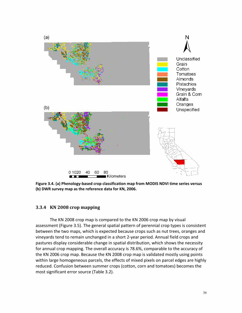
36

Figure 3.4. (a) Phenology-based crop classification map from MODIS NDVI time series versus (b) DWR survey map as the reference data for KN, 2006.

3.3.4 KN 2008 crop mapping

The KN 2008 crop map is compared to the KN 2006 crop map by visual assessment (Figure 3.5). The general spatial pattern of perennial crop types is consistent between the two maps, which is expected because crops such as nut trees, oranges and vineyards tend to remain unchanged in a short 2-year period. Annual field crops and pastures display considerable change in spatial distribution, which shows the necessity for annual crop mapping. The overall accuracy is 78.6%, comparable to the accuracy of the KN 2006 crop map. Because the KN 2008 crop map is validated mostly using points within large homogeneous parcels, the effects of mixed pixels on parcel edges are highly reduced. Confusion between summer crops (cotton, corn and tomatoes) becomes the most significant error source (Table 3.2).

37

The MLC for KN 2008 uses parameters trained from the same three training sets as used in the maximum classification of KN 2006. All available ground truths from fieldwork are employed for validation and low overall accuracies are achieved for all groups (64.1% for the 50% training set group, 60.7% for the 20% group and 52.7% for the 10% group). The poor performance suggests that the MLC fails to yield consistent outputs as a result of the inter-annual variation. Confusion matrices are not presented here due to low accuracies.

Figure 3.5. Phenology-based crop classification map for KN, 2008.

Table 3.2. Confusion matrix for the PBC in KN, 2008.

Mapped classes Ground truths Total User’s accuracy

Others Gr Ct Cr Af T Am P O V GC

Unclassified 39 1 2 1 3 2 11 6 3 9 3 80 Grain (Gr) 10 12 1 1 1 25 48% Cotton (Ct) 3 84 1 1 89 94% Corn (Cr) 3 2 28 4 1 1 2 2 43 65% Alfalfa (Af) 6 81 87 93% Tomatoes (T) 6 4 14 24 58% Almonds (Am) 10 2 123 10 1 146 84% Pistachios (P) 56 6 62 90% Oranges (O) 2 58 60 97% Vineyards (V) 2 1 4 6 2 45 60 75% Grain & Corn (GC) 6 2 4 3 15 30 50%

Total 85 13 91 37 94 16 142 79 65 64 20 706

Producer’s accuracy 46% 92% 92% 76% 86% 88% 87% 71% 89% 70% 75% Overall accuracy=78.6%. Kappa coefficient=0.76.

38

3.3.5 SJV 2007 crop mapping

For the entire SJV, a pixel-wise accuracy assessment of the 2007 crop classification is performed using the preprocessed CDL, which is the only state-wide reference dataset. The overall accuracy is 74.6%, which is acceptable for a large area. The confusion matrix (Table 3.3) is similar to the matrices of the PBC approach in the two counties. The classification map by PBC is compared to the CDL in 2007 (Figure 3.6).

39

Figure 3.6. PBC crop map versus CDL of the San Joaquin Valley, 2007.

40

Table 3.3. Confusion matrix for the phenology-based classification in the San Joaquin Valley, 2007.

Mapped classes Ground truths Total User’s accuracy

Gr Ct Af T Am O V GCC Unclassified 1292 535 1807 233 1939 258 1736 2689 10489 Grain (Gr) 9055 82 1381 25 380 15 113 834 11885 76% Cotton (Ct) 306 22811 777 185 470 1 382 659 25591 89% Alfalfa (Af) 492 436 24911 91 386 27 183 799 27325 91% Tomatoes (T) 195 512 348 2065 257 3 379 1052 4811 43% Almonds (Am) 510 161 1144 89 19215 142 602 583 22446 86% Oranges (O) 134 24 454 7 1290 1973 283 266 4431 45% Vineyards (V) 272 576 1342 168 2156 77 13493 715 18799 72% Grain & Corn or Corn (GCC) 1138 566 1130 334 750 3 363 13711 17995 76% Total 13394 25703 33294 3197 26843 2499 17534 21308 143772 Producer’s accuracy 68% 89% 75% 65% 72% 79% 77% 64% Overall accuracy=74.6%. Kappa coefficient=0.70.

3.4 Discussion

The PBC approach developed in this paper is compared to the traditional MLC approach focusing on advantages and disadvantages of the new approach. Accuracies of all the classifications performed in this study are summarized in Table 3.4. The best map produced by the MLC has a slightly higher accuracy than the map by the PBC approach, which suggests that the new PBC approach makes few improvements when available ground truth points are sufficient. However, when the size of the training set is limited by the amount of ground truth reference data, the two approaches behaves differently. With a training set smaller than approximately 10% of the study area, the MLC approach could not achieve an acceptable accuracy. In contrast, the PBC approach has few requirements on the size of training set, because this approach relies mostly on the knowledge of crop calendar and phenological transitions and only a very small set of ground truth reference points (in this study, only about 10 pixels for each crop type) are used to interpret typical NDVI profiles. Therefore, compared to the traditional MLC, the PBC approach developed in this study shows greater capacity in crop identification when using a minimum of ground truth reference data. This capacity could highly reduce the cost and the time of crop mapping, providing great potential for timely agricultural monitoring and management based on free remotely sensed data.

41

Table 3.4. Classification accuracies (in percentage) for different combinations of approaches and study areas.

PBC MLC

All pixels Classified pixels only 10:90 20:80 50:50 ME 2002 70.1 82.9 66.8 75.6 80.1 KN 2006 75.0 88.7 58.5 72.4 81.4 SJV 2007 74.6 KN 2008 78.6 52.7 60.7 64.1

The confusion matrices generated by the two approaches are examined in the evaluation of the classification performance. The two approaches generate distinct confusion matrices even when the overall accuracies are comparable. The confusion matrices of the PBC contain a considerable proportion of unclassified pixels, while the confusion matrices of the MLC have mostly inter-class confusion. By visual observation it is found that mixed pixels on parcel edges tend to be unclassified in the PBC. However, in the MLC, the probability threshold could be set to a low value and so these mixed pixels could be classified though the chance of commission error is increased. As a feature of the MLC, the adjustable probability threshold provides great flexibility in producing output maps with a desirable proportion of classified pixels. In comparison, the PBC always has strict criteria in recognizing crop types, which reduces the risk of misclassification as well as increasing the number of unclassified pixels. Compared to MLC, the PBC approach shows great performance in the classification of some specific crop types. As discussed above, the annual NDVI profile of alfalfa is clearly characterized by multiple short growing periods resulting from frequent cuts. However, the timing of cuts is highly flexible based on our experience. As a result, the NDVI peak of an alfalfa pixel may temporally coincide with the valley of another alfalfa pixel (Figure 3.7). In this case, the assumption of central tendency, which is the base of MLC, is likely to fail. The average NDVI profile of alfalfa employed in MLC had much less variation than individual alfalfa profiles (Figure 3.7) and thus a considerable number of pixels with high average NDVI and low variation are misclassified as alfalfa. By contrast, the PBC approach gets rid of this problem by capturing the pattern of individual alfalfa NDVI profiles. The PBC approach is also advantageous for recognizing crop types with normal NDVI profiles because phenological metrics instead of the original NDVI values are employed to account for the seasonal variation. In the study area, corn pixels generally have two typical NDVI profiles: one starts growing at DOY of ~110 and the other as late as ~150 (Figure 3.8). The difference results from varied practices, for example, the existence of rotational grain ahead of corn growth in some parcels may delay the corn season. During the period between the two different starting DOYs the NDVI value for corn is either very high or very low, which causes the assumption of central tendency to fail. In PBC, the difference is just considered as a shift of the growing season NDVI profile that could be easily represented by the ranges of the phenological metrics used in the decision trees. Therefore, the PBC approach possesses great advantages in identifying crop types with varied NDVI profiles.

42

Figure 3.7. NDVI profiles of three individual alfalfa pixels (diamonds connected with solid lines in red, green and blue respectively) and average NDVI profile of all alfalfa pixels (thick black line). Differences in temporal NDVI variation could be observed among the three profiles. The average profile shows low seasonal variation, which is significantly different from individual profiles.

Figure 3.8. NDVI profiles of two pixels with corn growth represented by diamonds connected with dashed lines. The solid lines are curves fitted to NDVI profiles in the growing season(s). The red profile belongs to a pixel with only corn grown in the year. The blue profile shows that in the other pixel grain is planted ahead of corn which delays the corn season.

ND

VI

1.0

0.8

0.6

0.4

0.2

0.0DOY

3002001000

ND

VI

1.0

0.8

0.6

0.4

0.2

0.0

DOY3002001000

43

The PBC approach maintains high classification accuracies across the entire study area and all years using the same setting of decision trees. Because only metrics related to phenology and plant vigor are used and effects of other factors are excluded in the classification, this approach is temporally stable given that the inter-annual phenological differences of the crop types fall within a reasonable range. In contrast, the MLC of the KN 2008 imagery using parameters trained from the 2006 ground truth reference data yields unacceptable accuracy. The parameters trained by the 2006 ground truth reference data represent all the surface characteristics displayed by the imagery, some of which are irrelevant to crop types, so the 2008 classification tends to be adversely affected by the inclusion of the year-specific factors such as precipitation and off-season land use. While the MLC of crop types is limited by the use of parameters trained with data of another year, the PBC approach is able to overcome this shortcoming by isolating the crop-specific surface characteristics. In addition, in the case of considerable change in phenological response or the inclusion of new interested crop type, the PBC approach could easily accommodate the new situation by adjusting the relevant nodes of the decision tree without altering the remaining invariant parts.

3.5 Summary

This study attempts to produce low cost annual cropland map of major specific crop types in SJV (south part of the Central Valley), California. MODIS data product MOD09Q1 proves to be a suitable data source to capture the NDVI profile characteristics of major crop types. The PBC classification approach proposed in this study, which uses phenological metrics derived by curve fitting of NDVI profiles as the data input and decision tree created mainly based on the local crop calendar as the classifier, provides us with reliable annual crop maps of major crop types. Cropping patterns are well portrayed by these crop maps. The PBC approach achieves high accuracy as well as reduces the requirement for large training datasets. Given knowledge of the crop calendar, agriculture practices and regional and climate variation, the PBC approach can be hopefully applied to the entire Central Valley, California. The 250 m spatial resolution of MODIS data still limits the further improvement of classification accuracy due to the effects of mixed pixels on parcel edges. Efforts in pixel unmixing could be made to extend the use of PBC approach to small parcels.

44

Chapter 4. Improved phenology based classification approach for agricultural water use estimate in high heterogeneity cropland

4.1 Background

The phenology based classification (PBC) approach is advantageous for its flexibility to adapt to various weather and agricultural conditions. The small parcel size of some counties’ cropland is the most limiting factor of PBC application in the entire Central Valley. The replacement of MODIS 250 m imagery with finer spatial resolution data is unavoidable in the mapping of patchy fields. In addition, as more specific crops are considered when the study area is extended, the usage of spectral characteristics is necessary in the identification of crops with similar growing seasons. Spectral signatures traditionally employed are associated with dates of imaging, which are absent in PBC. Incorporating spectral metrics in the PBC approach becomes a challenging task. The objective of the study in this chapter is to develop an effective and efficient method to identify major crop types in the Stanislaus County, California and create crop maps on an annual basis. Efforts in Chapter 3 have established a framework of MODIS inputs and a phenology-based classifier. According to the local conditions and the need for efficiency, several improvements have been made. 1) Landsat 5 TM and Landsat 7 ETM+ imagery is used to replace MODIS as the input to the classification algorithm. Landsat imagery is at a much finer spatial resolution (30 m, compared to MODIS’ 250 m resolution), which enables detailed crop mapping for smaller agricultural land parcels. 2) Metrics related to spectral information are incorporated. Previously only NDVI time series calculated from the red and near-infrared bands is utilized to derive phenological metrics. In the improved method, NDVI is replaced with enhanced vegetation index (EVI), which requires an additional blue band containing soil information. Reflectance of certain spectrum at certain growth stages is used in addition to previous phenological metrics to enhance the identification of some crop types. 3) The techniques of image segmentation and object based classification are utilized to reduce computational time and improve map quality. The method is summarized in the following section with a focus on new features of the algorithm.

4.2 Materials and methods

4.2.1 Study area

This study is focused on the total agricultural area of the Stanislaus County, California, which is in the middle of the Central Valley (center coordinates are approximately 37.5°N, 121°W). This area has vast flat terrain, deep soil, and a Mediterranean climate with hot dry summers and cool rainy winters. Annual precipitation is ~330 mm and is concentrated in the period of November to March. Both

45

the crop area and the economic value of agricultural products maintain a steady increasing trend during recent years. The area of Stanislaus County is 392,300 ha, and the total harvested area in year 2010 exceeds 420,000 ha as a result of multiple cropping. Similar to other areas in the Central Valley, crop types and growing pattern in Stanislaus County are diverse. Major crop types in Stanislaus County include (in order of total crop area): almond, corn, alfalfa, winter grain (wheat, oat and other winter grain forage), irrigated pasture, tomato, walnut, dry beans (including black-eyes, baby limas and large limas), and vineyard. These crop types comprise ~ 88% of the agricultural land. Rangeland is not included in the statistics and the classification because actual water use of rangeland is usually much lower than ideal water demand and calculated using other means.

4.2.2 Data

4.2.2.1 Landsat imagery

Stanislaus County is entirely enclosed in a Landsat tile (path 43, row 34). Two years, 2004 and 2010, are selected as study years to make use of the available field survey data. Landsat 5 TM and Landsat 7 ETM+ imagery are acquired from US Geological Survey (http://glovis.usgs.gov/). To capture the growth activity of both winter and summer crops, the time range of images used in crop mapping is set to an extended year instead of the calendar year. The beginning date is the day of year (DOY) 300 in the year prior to the target year. The end date is at the beginning of the following year, and the exact DOY depended on image quality. In year 2004 a total of 18 TM images and 21 ETM+ images are acquired and processed. In year 2010, 17 TM images and only 16 ETM+ images are available (Figure 4.1). Images are selected as long as part of Stanislaus’ cropland is cloud-free no matter how large the cloud-free area was. Although most of the images are geo-corrected, some images have insufficient ground control points due to partial cloud cover so manual geo-referencing is done. Radiometric calibration and atmospheric correction for cloud and aerosol effects are performed using Landsat Ecosystem Disturbance Adaptive Processing System by the US National Aeronautics and Space Administration (NASA) (Masek et al., 2006). Even though the use of Landsat imagery is maximized, some gaps between available images are still wide and affect the capacity to detect key phenological transitions. In this case, MODIS surface reflectance images are downscaled to 30 m resolution to fill gaps in the input dataset.

46

Figure 4.1 DOYs of images used in 2004 and 2010 Stanislaus crop mapping. Bars above the time line represent Landsat 5 TM images while bars below represent Landsat 7 ETM+ images. Black arrows indicate the time of the downscaled MODIS image used to fill the temporal gap of Landsat imagery.

4.2.2.2 MODIS reflectance (MOD09) imagery

MODIS 250 m and 500 m daily surface reflectance imagery are acquired from NASA’s Earth Observation System Warehouse Inventory Search Tool (discontinued, updated data sources are at https://lpdaac.usgs.gov/). The 250 m surface reflectance product (MOD09GQ) includes red and near-infrared bands and the 500 m surface reflectance product (MOD09GA) provides multispectral data ranging from optical to shortwave infrared bands. The wavelength of the MODIS bands are comparable to the corresponding Landsat bands, which makes the data fusion possible. MODIS images are corrected for the effects of atmosphere, dynamic aerosol and cirrus clouds before acquisition. The entire Stanislaus County is covered by one scene of MODIS imagery (row 05 and path 08). Low cloud cover images around the target dates are selected based on the quality assessment flags embedded in the MODIS products. Operations of image subset, format conversion and reprojection are completed using the MODIS Reprojection Tool (https://lpdaac.usgs.gov/lpdaac/tools/modis_reprojection_tool). Data fusion between Landsat and MODIS imagery is performed by the Spatial and Temporal Adaptive Reflectance Fusion Model based on the assumption that the correlation between these two datasets was constant within a certain period (Gao et al., 2006). The “pseudo” images created from the downscaled MODIS data at the Landsat resolution are also labeled in the time axis of Figure 4.1.

47

4.2.2.3 Land use field data

The land use program of the California Department of Water Resources (CDWR) provides the agricultural land use data for all counties in California. Details of the land use program and data are given in Section 2.2.2.2. Land use survey data of Stanislaus County is available for years 2004 and 2010. Over half of the cropland parcels are smaller than a MODIS pixel at the maximum resolution of 250 m. Validation is performed using the land use survey data as ground references. Other documents and materials are also employed as additional information on ground reality. Annual crop reports from the Stanislaus County Agricultural Commissioner provide basic statistics of all crop types such as planted acreage and economic values (http://www.stanag.org/crop-reports.shtm). USDA NASS weekly Crop Progress & Condition Report includes crop growing progress along with weather conditions as an information source for crop phenology (http://www.nass.usda.gov/Statistics_by_State/California/Publications/Crop_Progress_&_Condition/). Although not used directly, USDA CDL is considered as a reference for some crop types. Part of the study area is also visited to acquire high reliability field data.

4.2.3 Method

4.2.3.1 Image segmentation

Cropland of the study area is first segmented into multi-pixel objects using the software Berkeley Image Segmentation (Clinton et al., 2010). With proper parameterization, homogeneous objects identified by the software resemble the actual field boundaries. To reduce the computation time, three images at key seasons are stacked as the input to the segmentation algorithm for each year: early spring, early summer and late summer, and exact dates depend on image quality. Multiple combinations of three parameters, threshold, shape and compactness, are tested to achieve the optimum result. Detailed description of the segmentation procedure and parameters are provided at the software website (http://www.imageseg.com). The combination finally selected is 5, 0.3, and 0.6 for threshold, shape, and compactness respectively. The value of threshold, which represents the number of segmentation iterations, is relatively low to adapt for small fields. As a result, large fields tended to be split into multiple parts which are inconsistent with the actual field boundary. This is not problematic since the objective of this study is classification instead of boundary delineation. With additional efforts of digitalizing high resolution images, actual field boundaries might be already available ahead of the classification process. The possibility of utilizing existing field boundaries to segment images and improve crop mapping accuracy is also explored. Two polygon datasets, the image segmentation result and actual field boundaries (referred later as “segmentation” and “boundary” respectively),

48

are input individually to compare the classification results with and without prior digitalization efforts.

4.2.3.2 Time series generation

Landsat and fused images are converted into time series for each individual object using input polygons. Cloud-covered and other low quality pixels are first masked out using the quality flags generated by the LEDAPS algorithm. The median value of pixels within an object is assigned to the entire object, and a blank value is assigned if no high quality pixels are available. All image bands at all dates are processed in this way to produce multi-band time series of objects with various lengths. Although previous studies commonly found false values in the time series (Pettorelli et al., 2005), based on my observation the time series which are produced are consistent and reliable so no additional treatment or smoothing is applied. Time series of three indices are derived from multi-spectral reflectance: enhanced vegetation index (EVI), normalized differential senescent vegetation index (NDSVI), and normalized difference tillage index (NDTI). EVI is designed for MODIS data to retrieve biomass signal while reducing background soil signals. Compared to the simpler normalized difference vegetation index (NDVI), which is used as the main index representing vegetation vigor in previous PBC trials in Chapter 3, EVI is less likely to be affected by problems of saturation in high vegetation cover regions and atmospheric effects (Huete et al., 2002). EVI is computed with Landsat multi-spectral surface reflectance bands as:

LBCBCBBBGEVI

+×−×+−

×=12314

34 (4)

where B1, B3, and B4 are Landsat surface reflectance of blue, red and near infrared bands respectively, L is the canopy background adjustment, C1, C2 are the coefficients of aerosol resistance term, and G is the gain factor. Values of 1, 6, 7.5 and 2.5 are used for L, C1, C2, and G respectively (Huete et al., 1997). EVI time series, considered as the seasonal profile of crop growth, is the only input to derive phenological metrics. NDSVI and NDTI correlate to residue cover which represents crop-specific responses to water content (Pena-Barragan et al., 2011, Van Deventer et al., 1997). NDSVI and NDTI are calculated following the equations:

35

35

BBBBNDSVI

+−

= (5)

75

75

BBBBNDTI

+−

= (6)

where B5 and B7 are surface reflectance of two Landsat shortwave infrared bands, band 5 and band 7. These two indices offer more possibility of identifying crops based on reflective characteristics of the short-wave infrared wavelength region.

49

4.2.3.3 Derivation of metrics for classification

4.2.3.3.1 Phenological metrics In PBC, time series formed by surface reflectance values are utilized to compute “phenological metrics” related to dates of crop growing progress, and a classifier is developed to work on phenological and other derived metrics to identify specific crop types. This is the major difference from traditional multi-temporal classification algorithms, which directly focus on the distribution of surface reflectance or vegetation indices. Phenological metrics are derived by fitting double asymmetric sigmoid functions (Equation (1)) to EVI profiles of multi-pixel objects. The entire EVI profile of an object is first recognized as one or more “increasing and decreasing” growth patterns (Zhong et al., 2011). An asymmetric double sigmoid function is fitted to each growth pattern with a non-linear least square method using the Gauss-Newton algorithm. Phenological metrics are computed based on the function parameters if the curve-fitting is successful. Phenological metrics extracted from the time series are built to represent various biophysical meanings related to phenological phases and transitions. The classification capacity of each metric or combination of metrics is evaluated for each specific crop type according to the well recognized crop calendars and agricultural practices in the study areas. Since most crop types usually have specific crop calendars, the dates of the phenological phases are relatively fixed. Di and Dd in Equation (1) are the inflection (steepest) points on the double sigmoid curves, or the maximum and the minimum points of the first derivative, respectively. Di is considered as the date when most leaves are likely to emerge. This date is temporally stable for various canopy densities. In addition, because Di is constrained by the entire shape of the phenology, it is less affected by noises (Fisher & Mustard, 2007). Similarly, Dd is the date with the most rapid decrease of leaf content. Generally Dd has the same advantages as Di, especially for field crops that are cultivated in a short time. Comparatively, Dd is more uncertain for trees because defoliation is gradual and the rate depends on weather conditions and water availability. Some useful phenological metrics are not directly available as function parameters. EVI profiles of some crops have multiple modes (growing cycles), and the number of modes (n) is indicative of the crop type. For example, crop rotation between wheat and corn usually has n=2. Another example is alfalfa, a major pasture in the study area which is characterized by multiple same-year planting/cultivation and short growing seasons (~2.5 months). The sowing dates are highly uncertain, distributing randomly within most of a year. Curve-fitting is not effective as a result of the short growing periods. While metrics derived from curve-fitting are not available, the value of n greater than 4 or 5 became a reliable criterion to identify alfalfa. Crops with stable crop calendars tend to maintain a high level of EVI for a certain period within the growing season. The difference (Dd - Di), which is the length of high EVI period (LHVP), is a good indicator of the length of growing season of different crops. LHVP is of great importance in recognizing crops with distinct lengths of growing season.

50

Higher order derivatives of the EVI profile also have the potential in representing phenological phases (Soudani et al., 2008). The four DOYs when the second derivative of the EVI profile reaches extrema are named with subscripts from 1 to 4 and listed in the following equations:

226ln1

226ln1

226ln1

226ln1

4

3

2

1

−−=

−+=

−−=

−+=

qDD

qDD

pDD

pDD

d

d

i

i

(7)

All terms are defined previously. The first point, D1, was selected as an indicator of the onset of greenness and the fourth point, D4, was selected as an indicator of the onset of dormancy/fallow. The time between D1 and D4, (D4-D1), was defined as the length of the growing season (LGS) (Figure 1.1). These metrics were used in crop mapping when they have higher accuracy in characterizing crop growth than Di, Dd and LHVP.

4.2.3.3.2 Spectral metrics The improved PBC approach also employs multi-spectral metrics to identify most crop types. The major difference from traditional method is that all spectral metrics are related to specific phenological stages. In traditional studies, multi-spectral signatures of various crop types are only compared within one image at one time. The same crop at different growing stages might show distinct multi-spectral signatures and result in intra-class variability. Our PBC approach first creates time series of multi-spectral surface reflectance, NDSVI and NDTI. At DOYs indicated by phenological metrics, interpolated values of the time series are used as the spectral metrics at certain phenological stages. Spectral metrics with phenology are more comparable among crop types, because a crop type tends to have stable and consistent multi-spectral signatures at the same growing stage rather than at the same imaging date. In this way the impact of growing season variation on classification is potentially eliminated and crop-specific spectral information is isolated from temporal information. Spectral metrics tested in this study include red band reflectance (R), near infrared band reflectance (N), EVI (V), NDSVI (S), and NDTI (T), and subscripts from 1 to 4 are associated to indicate corresponding phenological stages from D1 to D4. Figure 4.2 is an example for the generation and use of spectral metrics. Spectral metrics possess the potential to classify crops with very similar crop calendars, for example, summer crop types including corn, dry beans and tomato.

51

Figure 4.2. An example of two crop types’ spectral metric profiles shows the advantage of PBC. The x-axis is DOY with two imaging dates marked with dotted lines. The y-axis is EVI. Two profiles of vineyard with a shift in green-up time (named vineyard 1 and vineyard 2 respectively) are drawn with dashed lines and one profile of walnut is drawn with a solid line. If the EVI of the two imaging dates are clustered to classify the three profiles, walnut is likely to be confused with vineyard 2. In PBC, the EVI of three profiles at D1 (marked with solid circles) are compared and the two types can be distinguished based on the EVI at the specific growth stage, which is V1.

4.2.3.4 Decision tree classifier

All the derived phenological and spectral metrics could be linked to crop calendar and physiological characteristics. A decision tree is established to classify crop types using rules on two sets of metrics. Thresholds of decision tree nodes are determined mainly based on previous decision trees built for neighboring areas with similar crop calendars and agricultural practices (Zhong et al., 2011). For spectral metrics newly added to PBC, multi-spectral time series are interpreted visually to find the approximate ranges of these metrics for crop types. An identical decision tree is applied to object metrics in both years 2004 and 2010 because no noticeable difference is observed from the USDA Crop Progress & Condition Reports. One problem with this approach is that the accuracy assessment tends to be slightly biased because the entire land use survey dataset is used as the test set, but part of the ground truth data is already used to determine threshold values of spectral metrics. However, this effect is trivial because the small number of ground truth points used for decision tree construction can be neglected.

52

The final decision tree is designed in a hierarchical manner. EVI profiles are split into individual growth modes. Temporal lengths of the growth modes are estimated by the starting and end DOYs. Alfalfa is identified according to the number of short growth modes in the profile. For other objects each growing mode is assigned to three general crop categories using the time range of growing seasons indicated by phenological metrics. The three crop categories include: winter crops, summer crops and tree crops & pasture. A pool of phenological and spectral metrics is tested to find proper threshold values to identify crop types according to the physical background of metrics.

4.2.3.5 Calculation of ETc for crop types

The FAO 56 method is used to calculate the crop evapotranspiration (ETc) rate for each crop type (Allen et al., 2005, Allen et al., 1998). The ETc rate at ideal condition without water stress is computed as the product of reference evapotranspiration rate (ETo) and crop coefficient (Kc). For the purpose of water planning, water demand should always be met so the maximum possible ETc under ideal irrigation and growth conditions is assumed to be the planned water use. The units for evapotranspiration rate and evapotranspiration (water use) volume are millimeter and hectare-meter respectively by default. In reality instantaneous ETc is influenced by irrigation (schedule and equipment type) and precipitation and Kc profiles may show spikes and valleys. These effects are neglected in the estimate of ideal ETc rate, and seasonal Kc is modeled by smooth curves only depending on season and crop type (Allen et al., 1998). Daily ETo of California at a 2 km resolution is provided by the California Irrigation Management Information System of CDWR as a spatial product interpolated from a network of weather stations, where ETo is calculated using the Penman-Monteith equation (http://wwwcimis.water.ca.gov/). The spatial resolution of 2 km is sufficient for the study area as a result of flat valley floor terrain and homogeneous weather conditions. The volume of ETc is calculated by multiplying ETc rate and area. The time range of monthly ETc calculation is set using the concept of water year, which is from October in the previous calendar year to September in the current calendar year (October 2003 to September 2004 and October 2009 to September 2010 for this study). Water years are commonly used in water planning and consistent with the growing seasons of crops mapped in the Central Valley.

4.2.3.6 Accuracy assessment

ETc calculated using the classified and true crop types is compared to evaluate the effect of classification error on the estimate of crop water use. The comparison between monthly ETc of classified types on the crop map (Em) and ETc of true crop types (Et) includes three quantitative measurements of model accuracy: root-mean-square error (RMSE), slope and r-square of regression. The equation of RMSE is:

53

∑=−=

n

i itim EEn

RMSE1

2,, )(1 (8)

where n is the total number of image objects or land parcels. RMSE is a widely used measure to compare differences between model predictions and observed data and has the same unit as original data. To estimate Et with Em, the regression relationship of Et = bEm is assumed where b is the slope. The intercept is set to 0 because no systematic bias should be involved in such a comparison. Both b and the r-square value (r2) are computed with the least square method. Values of b and r2 are supposed to approach one if Em is close to Et. Annual ETc as the total of monthly ETc in a water year is compared in the same manner.

4.3 Results

4.3.1 Decision tree modeling

In the final decision tree constructed manually through a trial-and-error process, alfalfa is first identified using the criteria of more than four short growth cycles (length > 60 days). For remaining single growth modes, the crop category is identified using phenological metrics and further divided into specific crop types with a selection of phenological or spectral metrics and proper cutting thresholds (Figure 4.3). Grain is the only winter crop and it is easily distinguished from other types. There is no need to separate specific winter grain types due to their similar water uses. Three summer crop types, corn, tomato and dry bean have very similar crop calendars and one branch of the decision tree effectively classifies these crops. Based on our observation, tomato has higher red band reflectance at the mature stage than corn and dry bean. Because the absolute value of red band reflectance is small (<0.1) and likely to be affected by noise, the relative magnitude of red band reflectance compared to blue band reflectance is employed to reduce the noise effect and improve the robustness. A new spectral metric IGS was developed as the maximum interval between red and blue band reflectance during the growing season from D1 to D4. Dry bean is characterized by high base VI levels and corn tends to show high NDSVI during early season. Thus, the metrics IGS, Vb and S2 are mainly used to classify the three summer crop types. The category trees & pasture includes all types maintaining high level EVI for most time of the year. EVI of irrigated pasture starts increasing in early spring when tree crops are still in dormancy. Slight differences exist among the green-up dates of tree crops. Walnut and vineyard have similar calendars so EVI, NDTI and reflectance at certain stages are used to distinguish these two types. Crop classification maps of year 2004 and 2010 are presented in Figure 4.4 and Figure 4.5 respectively.

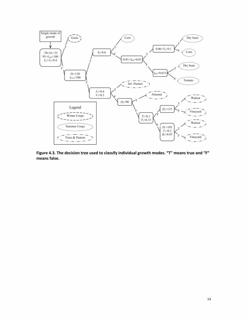
54

Figure 4.3. The decision tree used to classify individual growth modes. “T” means true and “F” means false.

55

Figure 4.4. Stanislaus crop classification map in 2004.

56

Figure 4.5. Stanislaus crop classification map in 2010.

4.3.2 Accuracy assessment

Accuracy assessment of the imagery classification mapping is performed based on the confusion matrix. For each of the four combinations of study years (2004 or 2010) and vector inputs (“segmentation” or “boundary”), two confusion matrices are created for the assessments by the number of polygons and by area respectively. Patterns of confusion matrices are similar and the combination of 2010 segmentation is given as an example (Table 4.1 and Table 4.2). Overall accuracies of all combinations are summarized along with the three quantitative measurements from the comparison between two ETc datasets (Table 4.3). If field boundaries are available, the area-based accuracy is consistently higher than classification using the segmentation result as the vector input. With existing field boundaries the chance of incorrectly classifying large fields is reduced.

57

Table 4.1. Polygon-based confusion matrix of year 2010 classification using segmentation result as vector input.

User classes

Ground-truth classes

Total User’s accuracy

Summer crops Trees & pasture

1 2 3 4 5 6 7 8 9 Unclassified 315 166 155 108 2448 405 215 176 561 4549 Grain(1) 1487 455 68 13 351 118 26 220 545 3283 45.3% Corn(2) 616 6451 469 130 131 51 54 137 709 8748 73.7% Dry bean(3) 30 85 477 184 2 3 4 22 807 59.1% Tomato(4) 39 136 255 709 86 50 54 9 75 1413 50.2% Almond(5) 21 32 3 2 5897 165 17 117 48 6302 93.6% Walnut(6) 5 238 1105 37 7 8 1400 78.9% Vineyard(7) 6 23 4 16 417 607 364 20 21 1478 24.6% Pasture(8) 3 26 2 563 23 617 91.2% Alfalfa(9) 11 25 10 1 41 1754 1842 95.2% Total 2525 7381 1431 1162 9606 2506 768 1292.7 3766 30438 Producer’s Accuracy 58.9% 87.4% 33.3% 61.0% 61.4% 44.1% 47.4% 43.6% 46.6% Overall accuracy=61.8%. Numbers in the matrix are polygon counts. Bold values correspond to number of polygons correctly identified.

Table 4.2. Area-based confusion matrix of year 2010 classification using segmentation result as vector input.

User classes Ground-truth classes

Total User’s accuracy

Summer crops Trees & pasture

1 2 3 4 5 6 7 8 9

Unclassified 971 441 489 294 9867 1326 1052 467 1267 16174

Grain(1) 4378 1096 176 15 1443 485 171 562 1487 9813 44.6%

Corn(2) 1749 18290 1804 477 416 167 182 338 1885 25308 72.3%

Dry bean(3) 86 259 2340 813 14 4 8 56 3580 65.4%

Tomato(4) 107 346 831 2871 315 130 233 16 159 5008 57.3%

Almond(5) 44 75 3 3 28994 557 89 308 141 30214 96.0%

Walnut(6) 10 933 3847 135 14 17 4956 77.6%

Vineyard(7) 20 55 7 44 1525 2126 1565 39 36 5417 28.9%

Pasture(8) 3 96 12 1567 43 1721 91.1%

Alfalfa(9) 24 37 32 1 128 5698 5920 96.3%

Total 7379 20612 5650 4517 43635 8654 3428 3447 10789 108111 Producer’s Accuracy 59.3% 88.7% 41.4% 63.6% 66.4% 44.5% 45.7% 45.5% 52.8% Overall accuracy=64.3%. The unit in the matrix is Hectare. Bold values correspond to area of polygons correctly identified.

58

Table 4.3. Summary of four combinations of classification and ETc comparison

Year Vector input Overall Map

accuracy ETc comparison

Polygon-based

Area-based Oct Nov Dec Jan Feb Mar Apr May Jun Jul Aug Sep Annual

2004

Boundary 64.7% 69.7% b 0.99 0.95 0.89 0.76 0.68 0.80 0.89 0.98 0.99 0.99 0.99 0.99 1.01

r2 0.91 0.78 0.67 0.72 0.65 0.77 0.88 0.94 0.93 0.94 0.87 0.88 0.97

RMSE 0.43 0.24 0.16 0.15 0.33 0.67 0.72 0.66 0.98 1.01 1.18 0.82 3.70

Segmentation 58.5% 61.4% b 1.01 1.00 0.89 0.63 0.52 0.80 0.91 1.00 0.99 0.99 0.99 1.00 1.02

r2 0.86 0.77 0.56 0.59 0.50 0.79 0.91 0.94 0.88 0.89 0.85 0.85 0.95

RMSE 0.31 0.14 0.09 0.09 0.20 0.35 0.34 0.38 0.71 0.74 0.72 0.54 2.76

2010

Boundary 66.4% 70.4% b 1.00 0.97 0.86 0.78 0.70 0.91 0.96 1.00 0.99 0.98 1.00 1.00 1.02

r2 0.90 0.78 0.61 0.71 0.66 0.86 0.93 0.95 0.93 0.93 0.91 0.90 0.96

RMSE 0.45 0.23 0.14 0.12 0.25 0.49 0.51 0.59 1.00 1.06 1.01 0.78 3.94

Segmentation 61.8% 64.3% b 1.01 0.97 0.87 0.76 0.67 0.89 0.96 1.00 0.99 0.98 0.99 1.01 1.03

r2 0.89 0.72 0.52 0.67 0.63 0.83 0.93 0.95 0.92 0.92 0.89 0.89 0.96

RMSE 0.16 0.08 0.05 0.04 0.08 0.17 0.16 0.19 0.33 0.34 0.34 0.26 1.31 The unit of RMSE is Hectare-meter.

4.4 Discussion

Confusions are found in the confusion matrices as shown by low user’s or producer’s accuracy less than 60%. Major confusions are analyzed one by one and possible reasons are explored. 1) Tree crops classified incorrectly or unclassified. According to our field visits, planting cover crops for orchard trees is a common agricultural practice especially for young trees. Cover crops are field crops grown between tree intervals in order to improve soil health and fertility, increase water retention, etc. The growing season of cover crops is from the rain period in later winter or early spring to the date before tree green-up when cover crops are usually plowed to increase water availability for trees, which coincides with the growing season of winter grain. The species and planting manners of cover crops are highly diverse so it is impossible to model cover crops in the decision tree. Young trees are hard to identify due to low EVI, and only cover crops contribute to the seasonal profiles of these fields. During recent years the area of orchard trees has been increasing significantly due to economic factors, and young tree fields keep emerging. Some of the young tree fields are recorded in the survey and excluded from the ground reference dataset, however, the record is not complete and only includes very young trees. The other special condition is very old trees, which are no longer irrigated for production. Although usually removed, these old trees can be left in fields and have an incomplete growing signal that is easily confused with summer crops. 2) Irrigated pasture classified incorrectly or unclassified. Although fields of irrigated pasture are available from the land use survey, irrigated pasture is not a crop type strictly defined. This type includes a vast variety of pasture species, among which the majority maintains high EVI level during most of the year while some species may

59

show totally distinct growing patterns. The situation is further complicated by the fact that pasture fields often contain a mixture of two or more plants including alfalfa, silage corn, sudan grass, winter grain, etc. Some fields are irrigated well while others show considerable water stress. Due to these factors there is a high chance to confuse irrigated pasture with other types. More detailed field information is required to improve the identification of irrigated pasture. 3) Alfalfa classified as winter grain or summer corn. Alfalfa is classified using the characteristics of multiple short growing cycles. Exceptions occasionally occur when alfalfa fields are not harvested periodically. As a result, the longer growing season is similar to winter or summer field crops. So far alfalfa cannot be identified using spectral metrics because the spectral signature of alfalfa keeps changing with its rapid growth and the growing stage at the imaging date could not be possibly known. 4) Corn classified as winter grain. Double cropping of winter wheat or other grain crops and summer corn is very common around the study area. A majority of the corn fields have grain planted in winter, and these fields are still classified as corn because corn water use in summer is more crucial for water planning than winter water consumption of grain. The growing season length of corn is relatively fixed, however, early harvest for silage may also happen. If corn growth is not identified due to the short season, the field is classified as grain according to the winter crop cover. Although these confusions largely reduce the accuracy of image classification, the incorrectly classified or unclassified fields are not likely to bias the water use estimate. Unclassified fields reflect various special conditions (young/old trees, water stress, early cut, etc.) under which crop water consumption is much lower than the ideal level. In this case, crop types from PBC are even better representatives of the actual situation than the land use survey data. Some incorrect classification occurs when the actual seasonal growth as well as the water use of a crop field resembles another crop type. Most of the confusions not discussed above exist within crop categories, for example, tomato identified as dry bean, or walnut identified as almond. Such confusions will not significantly affect the water use estimate because crops within the same category have similar seasonal Kc. All three measurements (b, r2, and RMSE) indicate that the difference in water use between classified and true crop types is much less than suggested by the classification accuracy (Table 4.3) largely because of similar water use between crops in the major categories. b and r2 are close to one especially during the rainless period from April to September when irrigation and water allocation are applied. From November to March, the regression relationship is not as good possibly because of rainfall. However, crop water use during this period is usually directly from precipitation and has less meaning for water planning. Both the absolute magnitude of ETc and RMSE are low due to cold weather. Thus, it is believed that the crop map produced by the PBC approach could allow us to make reasonable estimates of both monthly and annual crop water use. Classification error is unlikely to result in significant deviation of ETc for the reason mentioned. ETc rate is computed as the product of the reference evapotranspiration rate (ETo) and Kc. Since the ETo calculation is independent of crop types, the effect of

60

classification error on ETc is analyzed by examining the seasonal Kc determined from classified and true crop types. Figure 4.6 gives an example of the comparison of year 2004 using bubble plots. It shows all bubble plots of year 2010 with the collected field data as the vector input because the selection of the field dataset is of higher reliability than the exhaustive land use survey. The centers of the circles are set according to Kc of classified and true crop types. The sizes of the circles represent the number of fields with the corresponding classified and true Kc. On the bubble plots all the large circles are close to the diagonal, suggesting closeness of the two sets of Kc. This figure shows that most misclassification of the crop types using PBC does not have a major effect on the estimate of Kc and also ETc.

Figure 4.6. Bubble plots of Kc from classified and true crop types for three selected months in 2004.

61

Figure 4.7. Bubble plots of Kc from classified and true crop types for water year 2010.

62

The PBC approach in this study is robust and is not likely to be affected by abnormal values in one or a few images. Regular use of this approach to annually estimate crop water use is feasible because the entire procedure relies on free imagery and requires no ground reference data. Cutting thresholds in the decision tree might need minor adjustments according to the Crop Progress & Condition Report under extreme weather conditions. For years when high resolution images are available, the input of field boundaries from digitalization is likely to improve the classification accuracy, though not required.

4.5 Summary

This study attempts to use the PBC approach to produce a low cost annual cropland map of specific crop types in Stanislaus County, California using free Landsat and MODIS imagery. The PBC approach is improved to represent growing season with phenological metrics and employs spectral metrics associated with phenological stages to extract stable spectral characteristics of crops. The PBC approach provides the possibility of regularly mapping crop types and estimating water use without collecting additional ground reference data for training. Given our knowledge of the crop calendar, agriculture practices and regional and climate variation, the PBC approach can be hopefully applied to the entire Central Valley, California. Crop water use computed using crop types and weather variables has high accuracy. Confusions in the PBC only have trivial effects on the estimate of water use because classification error only occurs between crop types with similar seasonal water use or actual water use of unclassified fields is much lower than the ideal level.

63

Chapter 5. Conclusion Classification accuracy is essential in evaluating the performance of a classifier. Traditional maximum likelihood classification is able to yield high accuracies when there is a large ground truth dataset for training. Such a dataset requires extensive field work and is only available for a certain area during limited periods. A hybrid classification approach is recommended which applies the maximum likelihood classifier when training data is sufficient and the phenology based classifier when ground truths are unavailable. The accuracies of PBC are slightly lower than the maximum accuracy achieved by the maximum likelihood classification. However, PBC consistently produces crop maps with acceptable accuracies even when the field knowledge is very limited. In addition to the mapping accuracy, the uncertainty in water use estimate is another measurement of concern in this study. Errors in the estimate of crop water use are not sensitive to mis-classification in PBC. This is because most confusion occurs among crop types with similar seasonal patterns of water consumption which only results in negligible errors in the estimate of agricultural water use. Unclassified fields by the PBC are generally caused by special crop conditions including young age, very sparse coverage and water stress, which actually reflect the reality of low water use. In general, the quality and the reliability of crop maps created by the classification approach used in this study are adequate for water planning as well as other purposes. Objectives of this study are examined to check if the development of the PBC approach proposed in Chapter 1 successfully meets project goals for accuracy, cost, computation time and minimization of field data collection. The cost of the entire classification process is controlled to a very low level. There is little expense on imagery purchase because the two major image sources, MODIS and Landsat TM/ETM+, are available for free. For the time of data processing, each county’s crop map can be produced in a few hours, which is acceptable. Most processing time is attributed to Landsat imagery correction and curve-fitting, and further optimization is suggested in future studies. Computational time of other procedures is negligible thanks to the high performance of the image segmentation algorithm and decision trees. Cost of labor is highly reduced as the entire crop mapping process is semi-automatic. The most remarkable improvement on efficiency is that there is no need to collect a large set of ground truth data, which usually takes considerable resources and several months’ time. Even for a new area, only a few field visits are sufficient to gain a basic understanding on the local cropland. Instead of field data collection, efforts are required to obtain current year’s planting and harvest calendars of major crop types. Information on crop progress, which is usually available from regular publications and documents provided by government agencies and consulting business, is the major source of crop calendars. Crop calendars tend to be stable only except for some years with extreme weather conditions. Based on the experience from applications in the Central Valley, once the crop calendars are known for an area, it is rarely necessary to make adjustments. Communication with local agricultural experts could provide supplemental information if required. In general, the cost of the PBC has been greatly reduced by eliminating the need of extensive field data collection.

64

For the purpose of transferability, the studies show that classification algorithm built for an area in a year could be easily “re-used” in another area or another year. The Central Valley has a flat terrain and a homogeneous climate pattern. Most of major crop types in the Central Valley distribute along a vast area, so the corresponding parts in the decision trees are almost universally usable. For example, almond, which is a common tree crop found in the entire Central Valley, could be treated with the same structure of nodes in the decision tree. Threshold values might be slightly different for a part of the criteria due to spatial heterogeneity. The Central Valley is a narrow area with a north-south direction, and thus temperature, which controls appropriate crop types, shows great spatial variance. The start of growing season (green-up dates of tree crops or planting dates of field crops) tends to be late in north and early in south, and the length of the growing season is usually shorter in the southern area due to sufficient heat. All these factors need to be handled by decision trees by applying various parameters to sub-areas separately. Hopefully with the inclusion of more universal metrics such as accumulated temperature, some crop types within the entire Central Valley could be identified using a uniform set of criteria (Zhang et al., 2009). However, at present adjustments to the decision trees are still necessary to accommodate the longitudinal variation in the valley area. The inter-annual transfer of classification algorithms and parameters is similar in which inter-annual variation is mostly caused by differences in temperature. The length of the rainy season (from late autumn to early spring) may also affect crop calendars. As long as the climate pattern and the manner of agricultural operation are well understood, the PBC could be applied to a large area for multiple years with few additional efforts. In order to avoid the loss of phenological and other information which occurs in the selective use of remotely sensed images in previous efforts, a “take-all” strategy is taken to include all available images in the classification even for images with considerable cloud cover. This strategy is uncommon in other studies because two problems may be caused: unacceptable high dimensionality and long computational time. In the exploration of this study, the problem of high dimensionality is solved by the curve-fitting technique, which is considered as a transformation approach with physical meanings. The curve-fitting technique also helps to reduce the time of calculation, along with the use of image segmentation and object-based classification. All these means enable PBC to take all available data as inputs without any negative effects. In addition, the usage of spectral information has been maximized by developing spectral metrics associated with phenological stages. Spectral signatures of crops tend to be stable at certain growing periods. Useless noise is removed by isolating crops’ spectral characteristics from image-specific signals. In this way, during the process of data assembling no image or useful metric is omitted and meanwhile it is ensured that all extracted metrics are related to crop types without over-fitting. Based on the evaluation above, the PBC successfully meets the need of large area annual crop mapping in the Central Valley with high efficiency and low cost. In order to extend the approach to the entire Central Valley or even the entire California, more knowledge should be gained regarding the agricultural customs to fully recognize the crop types. Attentions should be paid to three crop types or categories. i) Crops with

65

very flexible calendars (for example, carrots and onions) are not mapped in current PBC. Spectral metrics instead of phenological metrics may play an important role in the identification of such crop types. Hopefully by testing more spectral measurements or indices, proper metrics with the distinguishing capacity could be found. ii) Some crop types need to be re-defined or split to reduce the intra-class variation and improve the classification accuracy. For example, the type of mixed pasture contains various sub-types which need to be treated separately according to the pasture species, planting manner and irrigation condition. Another example is that different varieties of a crop type may display distinct phenological characteristics. Ideally a classification scheme is to be built to facilitate both crop identification and water use estimate. iii) A large number of specific crop types need to be handled when the crop mapping is extended to a larger area or to a more detailed level. Adding new crop types to existing decision trees is simple without altering original tree structures. Most efforts will be spent on examining new crop types’ crop calendars, common agricultural practices and spectral signatures. Future efforts will focus on the solutions of identifying these crop types or categories when crop mapping is extended to a larger extent and a finer scale.

66

References

Allen, R.G., Pereira, L.S., Raes, D., & Smith, M. (1998). Crop evapotranspiration: Guidelines for computing crop requirements.

Allen, R.G., Pereira, L.S., Smith, M., Raes, D., & Wright, J.L. (2005). FAO-56 dual crop coefficient method for estimating evaporation from soil and application extensions. Journal of Irrigation and Drainage Engineering-Asce, 131, 2-13

Anderson, M.C., Norman, J.M., Diak, G.R., Kustas, W.P., & Mecikalski, J.R. (1997). A two-source time-integrated model for estimating surface fluxes using thermal infrared remote sensing. Remote Sensing of Environment, 60, 195-216

Badhwar, G.B. (1984). Automatic corn-soybean classification using Landsat MSS data. II. Early season crop proportion estimation. Remote Sensing of Environment, 14, 31-37

Bastiaanssen, W.G.M., Menenti, M., Feddes, R.A., & Holtslag, A.A.M. (1998). A remote sensing surface energy balance algorithm for land (SEBAL) - 1. Formulation. Journal of Hydrology, 213, 198-212

Beck, P.S.A., Atzberger, C., Høgda, K.A., Johansen, B., & Skidmore, A.K. (2006). Improved monitoring of vegetation dynamics at very high latitudes: A new method using MODIS NDVI. Remote Sensing of Environment, 100, 321-334

Biggs, T.W., Thenkabail, P.S., Gumma, M.K., Scott, C.A., Parthasaradhi, G.R., & Turral, H.N. (2006). Irrigated area mapping in heterogeneous landscapes with MODIS time series, ground truth and census data, Krishna Basin, India. International Journal of Remote Sensing, 27, 4245-4266

Blaschke, T. (2010). Object based image analysis for remote sensing. Isprs Journal of Photogrammetry and Remote Sensing, 65, 2-16

Chen, J., Jonsson, P., Tamura, M., Gu, Z.H., Matsushita, B., & Eklundh, L. (2004). A simple method for reconstructing a high-quality NDVI time-series data set based on the Savitzky-Golay filter. Remote Sensing of Environment, 91, 332-344

Choudhury, I., & Chakraborty, M. (2006). SAR signature investigation of rice crop using RADARSAT data. International Journal of Remote Sensing, 27, 519-534

Clinton, N., Holt, A., Scarborough, J., Yan, L., & Gong, P. (2010). Accuracy Assessment Measures for Object-based Image Segmentation Goodness. Photogrammetric Engineering and Remote Sensing, 76, 289-299

67

Congalton, R., Balogh, M., Bell, C., Green, K., Milliken, J., & Ottman, R. (1998). Mapping and monitoring agricultural crops and other land cover in the Lower Colorado River Basin. Photogrammetric Engineering and Remote Sensing, 64, 1107-1113

De Fries, R.S., Hansen, M., Townshend, J.R.G., & Sohlberg, R. (1998). Global land cover classifications at 8 km spatial resolution: the use of training data derived from Landsat imagery in decision tree classifiers. International Journal of Remote Sensing, 19, 3141-3168

De Santa Olalla, F.M., Calera, A., & Dominguez, A. (2003). Monitoring irrigation water use by combining Irrigation Advisory Service, and remotely sensed data with a geographic information system. Agricultural Water Management, 61, 111-124

De Wit, A.J.W., & Clevers, J.G.P.W. (2004). Efficiency and accuracy of per-field classification for operational crop mapping. International Journal of Remote Sensing, 25, 4091-4112

Del Frate, F., Ferrazzoli, P., & Schiavon, G. (2003). Retrieving soil moisture and agricultural variables by microwave radiometry using neural networks. Remote Sensing of Environment, 84, 174-183

Dinar, A., & Zilberman, D. (1991). The Economics of Resource-Conservation, Pollution-Reduction Technology Selection - the Case of Irrigation Water. Resources and Energy, 13, 323-348

Doraiswamy, P.C., Hatfield, J.L., Jackson, T.J., Akhmedov, B., Prueger, J., & Stern, A. (2004). Crop condition and yield simulations using Landsat and MODIS. , 92, 548-559

El-Magd, I.A., & Tanton, T.W. (2003). Improvements in land use mapping for irrigated agriculture from satellite sensor data using a multi-stage maximum likelihood classification. International Journal of Remote Sensing, 24, 4197-4206

Erol, H., & Akdeniz, F. (2005). A per-field classification method based on mixture distribution models and an application to Landsat Thematic Mapper data. International Journal of Remote Sensing, 26, 1229-1244

Fisher, J.B. (2006). The land-atmosphere water flux across plant, ecosystem, global and social scales.

Fisher, J.I., & Mustard, J.F. (2007). Cross-scalar satellite phenology from ground, Landsat, and MODIS data. Remote Sensing of Environment, 109, 261-273

Friedl, M.A., & Brodley, C.E. (1997). Decision tree classification of land cover from remotely sensed data. Remote Sensing of Environment, 61, 399-409

68

Gao, F., Masek, J., Schwaller, M., & Hall, F. (2006). On the blending of the Landsat and MODIS surface reflectance: Predicting daily Landsat surface reflectance. IEEE Transactions on Geoscience and Remote Sensing, 44, 2207-2218

Haboudane, D., Miller, J.R., Tremblay, N., Zarco-Tejada, P.J., & Dextraze, L. (2002). Integrated narrow-band vegetation indices for prediction of crop chlorophyll content for application to precision agriculture. Remote Sensing of Environment, 81, 416-426

Hansen, M.C., Defries, R.S., Townshend, J.R.G., & Sohlberg, R. (2000). Global land cover classification at 1km spatial resolution using a classification tree approach. International Journal of Remote Sensing, 21, 1331-1364

Hoekman, S.K. (2009). Biofuels in the US - Challenges and Opportunities. Renewable Energy, 34, 14-22

Homer, C., Huang, C.Q., Yang, L.M., Wylie, B., & Coan, M. (2004). Development of a 2001 National Land-Cover Database for the United States. Photogrammetric Engineering and Remote Sensing, 70, 829-840

Huete, A., Didan, K., Miura, T., Rodriguez, E., Gao, X., & Ferreira, L. (2002). Overview of the radiometric and biophysical performance of the MODIS vegetation indices. Remote Sensing of Environment, 83, 195-213

Huete, A.R., Liu, H.Q., Batchily, K., & van Leeuwen, W. (1997). A comparison of vegetation indices over a global set of TM images for EOS-MODIS. Remote Sensing of Environment, 59, 440-451

Jakubauskas, M.E., Legates, D.R., & Kastens, J.H. (2001). Harmonic analysis of time-series AVHRR NDVI data. Photogrammetric Engineering and Remote Sensing, 67, 461-470

Le Toan, T., Ribbes, F., Wang, L.F., Floury, N., Ding, K.H., Kong, J.A., et al. (1997). Rice crop mapping and monitoring using ERS-1 data based on experiment and modeling results. , 35, 41-56

Loveland, T.R., Merchant, J.W., Ohlen, D.O., & Brown, J.F. (1991). Development of a Land-Cover Characteristics Database for the Conterminous United-States. Photogrammetric Engineering and Remote Sensing, 57, 1453-1463

Loveland, T.R., Reed, B.C., Brown, J.F., Ohlen, D.O., Zhu, Z., Yang, L., et al. (2000). Development of a global land cover characteristics database and IGBP DISCover from 1 km AVHRR data. International Journal of Remote Sensing, 21, 1303-1330

69

Luisa Castillejo-Gonzalez, I., Lopez-Granados, F., Garcia-Ferrer, A., Manuel Pena-Barragan, J., Jurado-Exposito, M., Sanchez de la Orden, M., et al. (2009). Object- and pixel-based analysis for mapping crops and their agro-environmental associated measures using QuickBird imagery. Computers and Electronics in Agriculture, 68, 207-215

Martinez-Casasnovas, J.A., Martin-Montero, A., & Casterad, M.A. (2005). Mapping multi-year cropping patterns in small irrigation districts from time-series analysis of Landsat TM images. European Journal of Agronomy, 23, 159-169

Masek, J., Vermote, E., Saleous, N., Wolfe, R., Hall, F., Huemmrich, K., et al. (2006). A Landsat surface reflectance dataset for North America, 1990-2000 RID F-3944-2010. Ieee Geoscience and Remote Sensing Letters, 3, 68-72

Murakami, T., Ogawa, S., Ishitsuka, N., Kumagai, K., & Saito, G. (2001). Crop discrimination with multitemporal SPOT. International Journal of Remote Sensing, 22, 1335-1348

Murthy, C.S., Raju, P.V., & Badrinath, K.V.S. (2003). Classification of wheat crop with multi-temporal images: Performance of maximum likelihood and artificial neural networks. International Journal of Remote Sensing, 24, 4871-4890

Myneni, R.B., Keeling, C.D., Tucker, C.J., Asrar, G., & Nemani, R.R. (1997). Increased plant growth in the northern high latitudes from 1981 to 1991. Nature, 386, 698-702

Norman, J.M., Kustas, W.P., & Humes, K.S. (1995). Source Approach for Estimating Soil and Vegetation Energy Fluxes in Observations of Directional Radiometric Surface-Temperature. Agricultural and Forest Meteorology, 77, 263-293

Olsson, L., & Eklundh, L. (1994). Fourier-Series for Analysis of Temporal Sequences of Satellite Sensor Imagery. International Journal of Remote Sensing, 15, 3735-3741

Pal, M., & Mather, P.M. (2006). Some issues in the classification of DAIS hyperspectral data. International Journal of Remote Sensing, 27, 2895-2916

Pena-Barragan, J.M., Ngugi, M.K., Plant, R.E., & Six, J. (2011). Object-based crop identification using multiple vegetation indices, textural features and crop phenology. Remote Sensing of Environment, 115, 1301-1316

Pettorelli, N., Vik, J.O., Mysterud, A., Gaillard, J.M., Tucker, C.J., & Stenseth, N.C. (2005). Using the satellite-derived NDVI to assess ecological responses to environmental change. Trends in Ecology & Evolution, 20, 503-510

70

Pinter, P., Ritchie, J., Hatfield, J., & Hart, G. (2003). The agricultural research service's remote sensing program: An example of interagency collaboration. Photogrammetric Engineering and Remote Sensing, 69, 615-618

Pu, R., Gong, P., Tian, Y., Miao, X., Carruthers, R.I., & Anderson, G.L. (2008). Using classification and NDVI differencing methods for monitoring sparse vegetation coverage: a case study of saltcedar in Nevada, USA RID A-6793-2010. International Journal of Remote Sensing, 29, 3987-4011

Sakamoto, T., Yokozawa, M., Toritani, H., Shibayama, M., Ishitsuka, N., & Ohno, H. (2005). A crop phenology detection method using time-series MODIS data. Remote Sensing of Environment, 96, 366-374

Shao, Y., Lunetta, R.S., Ediriwickrema, J., & Liames, J. (2010). Mapping Cropland and Major Crop Types across the Great Lakes Basin using MODIS-NDVI Data. Photogrammetric Engineering and Remote Sensing, 76, 73-84

Soares, J.V., Renno, C.D., Formaggio, A.R., Yanasse, C.D.C.F., & Frery, A.C. (1997). An investigation of the selection of texture features for crop discrimination using SAR imagery. Remote Sensing of Environment, 59, 234-247

Soudani, K., le Maire, G., Dufrene, E., Francois, C., Delpierre, N., Ulrich, E., et al. (2008). Evaluation of the onset of green-up in temperate deciduous broadleaf forests derived from Moderate Resolution Imaging Spectroradiometer (MODIS) data. Remote Sensing of Environment, 112, 2643-2655

Stehman, S.V., & Milliken, J.A. (2007). Estimating the effect of crop classification error on evapotranspiration derived from remote sensing in the lower Colorado River basin, USA. Remote Sensing of Environment, 106, 217-227

Thenkabail, P.S., Biradar, C.M., Noojipady, P., Dheeravath, V., Li, Y., Velpuri, M., et al. (2009). Global irrigated area map (GIAM), derived from remote sensing, for the end of the last millennium. International Journal of Remote Sensing, 30, 3679-3733

Tso, B., & Mather, P.M. (1999). Crop discrimination using multi-temporal SAR imagery. International Journal of Remote Sensing, 20, 2443-2460

Turker, M., & Arikan, M. (2005). Sequential masking classification of multi-temporal Landsat7 ETM+ images for field-based crop mapping in Karacabey, Turkey. International Journal of Remote Sensing, 26, 3813-3830

USDA. (2009). 2007 Census of Agriculture, California State and County Data, Volume 1, Geographic Area Series, Part 51 . National Agricultural Statistics Service, Washington, DC

71

USDA. (2004). 2002 Census of Agriculture, California State and County Data, Volume 1, Geographic Area Series, Part 51 . National Agricultural Statistics Service, Washington, DC

Van Deventer, A., Ward, A., Gowda, P., & Lyon, J. (1997). Using thematic mapper data to identify contrasting soil plains and tillage practices. Photogrammetric Engineering and Remote Sensing, 63, 87-93

Vandijk, A., Callis, S.L., Sakamoto, C.M., & Decker, W.L. (1987). Smoothing Vegetation Index Profiles - an Alternative Method for Reducing Radiometric Disturbance in Noaa/avhrr Data. Photogrammetric Engineering and Remote Sensing, 53, 1059-1067

Verhoef, W., Menenti, M., & Azzali, S. (1996). A colour composite of NOAA-AVHRR-NDVI based on time series analysis (1981-1992). International Journal of Remote Sensing, 17, 231-235

Vogelmann, J.E., Howard, S.M., Yang, L.M., Larson, C.R., Wylie, B.K., & Van Driel, N. (2001). Completion of the 1990s National Land Cover Data set for the conterminous United States from Landsat Thematic Mapper data and Ancillary data sources. Photogrammetric Engineering and Remote Sensing, 67, 650-662

Wade, G., Mueller, R., Cook, P., & Doraiswamy, P. (1994). AVHRR Map Products for Crop Condition Assessment - a Geographic Information-Systems Approach. Photogrammetric Engineering and Remote Sensing, 60, 1145-1150

Wardlow, B.D., Egbert, S.L., & Kastens, J.H. (2007). Analysis of time-series MODIS 250 m vegetation index data for crop classification in the US Central Great Plains. Remote Sensing of Environment, 108, 290-310

Xavier, A.C., Rudorff, B.F.T., Berka, L.M.S., & Moreira, M.A. (2006). Multi-temporal analysis of MODIS data to classify sugarcane crop. International Journal of Remote Sensing, 27, 755-768

Xiao, X., Boles, S., Liu, J., Zhuang, D., Frolking, S., Li, C., et al. (2005). Mapping paddy rice agriculture in southern China using multi-temporal MODIS images. Remote Sensing of Environment, 95, 480-492

Xie, H., Tian, Y.Q., Granillo, J.A., & Keller, G.R. (2007). Suitable remote sensing method and data for mapping and measuring active crop fields. International Journal of Remote Sensing, 28, 395-411

Zhang, X., Friedl, M.A., & Schaaf, C.B. (2009). Sensitivity of vegetation phenology detection to the temporal resolution of satellite data. International Journal of Remote Sensing, 30, 2061-2074

72

Zhang, X., Friedl, M.A., Schaaf, C.B., Strahler, A.H., Hodges, J.C.F., Gao, F., et al. (2003). Monitoring vegetation phenology using MODIS. Remote Sensing of Environment, 84, 471-475

Zhong, L., Hawkins, T., Biging, G., & Gong, P. (2011). A phenology-based approach to map crop types in the San Joaquin Valley, California. International Journal of Remote Sensing, 32, 7777-7804

Zhong, L., Hawkins, T., Holland, K., Gong, P., & Biging, G. (2009). Satellite imagery can support water planning in the Central Valley. California Agriculture, 63, 220-224

Zilberman, D., Macdougall, N., & Shah, F. (1994). Changes in Water Allocation Mechanisms for California Agriculture. , 12, 122-133