efficient 2d-to-3d correspondence filtering for scalable ... · efﬁcient 2d-to-3d correspondence...

Efficient 2D-to-3D Correspondence Filtering for Scalable 3D Object Recognition

Qiang Hao1∗, Rui Cai2, Zhiwei Li2, Lei Zhang2, Yanwei Pang1, Feng Wu2, Yong Rui2

1Tianjin University, Tianjin 300072, P.R. China2Microsoft Research Asia, Beijing 100080, P.R. China

1{qhao,pyw}@tju.edu.cn, 2{ruicai,zli,leizhang,fengwu,yongrui}@microsoft.com

Abstract

3D model-based object recognition has been a notice-

able research trend in recent years. Common methods find

2D-to-3D correspondences and make recognition decisions

by pose estimation, whose efficiency usually suffers from

noisy correspondences caused by the increasing number

of target objects. To overcome this scalability bottleneck,

we propose an efficient 2D-to-3D correspondence filtering

approach, which combines a light-weight neighborhood-

based step with a finer-grained pairwise step to remove

spurious correspondences based on 2D/3D geometric cues.

On a dataset of 300 3D objects, our solution achieves ∼10

times speed improvement over the baseline, with a compa-

rable recognition accuracy. A parallel implementation on a

quad-core CPU can run at ∼3fps for 1280×720 images.

1. Introduction

The recent progress in structure-from-motion (SfM)

techniques [22, 23, 26] has greatly facilitated 3D recon-

struction from unordered images. Reconstructed 3D models

characterize intrinsic geometric structures of objects, and

thus provide a compact and comprehensive object repre-

sentation with good generalization capability to unseen 2D

views. These advantages have inspired a trend of leveraging

3D models for recognition of rigid 3D objects [12, 16, 8],

especially landmarks [13, 15, 21, 9], appearing in images.

1.1. Object recognition by 2D-to-3D registration

Basically, this stream of work treats object recognition

in query images as a 2D-to-3D registration problem, which

aims to estimate the camera pose of a query image relative

to a 3D object model in mainly two stages as follows:

1) Identifying 2D-to-3D correspondences. A 3D model

consists of a set of 3D points, each of which is visu-

ally characterized by some local features, called model

features. Putative 2D-to-3D correspondences between the

∗This work was performed at Microsoft Research Asia.

��

��

��

Figure 1. Scalable 3D object recognition. Given many 3D object

models in the database as the targets, the task is to efficiently

recognize an arbitrary number of objects appearing in each query

image and estimate the pose for each identified object.

local features in a query image, called image features, and

the 3D points are identified by feature matching, which

is commonly accelerated by k-d tree based approximate

nearest neighbor (ANN) search [2].

2) Pose estimation for object recognition. After obtaining

putative correspondences, a minimal pose solver, e.g.,

Perspective-3-Point (P3P), is integrated with the RANSAC

paradigm [6] to estimate the camera pose. Object recog-

nition results are determined by the number of correspon-

dences that are consistent with the estimated pose.

The quality of putative 2D-to-3D correspondences is

crucial for such a framework. Specifically, the inlier ratio

(i.e., the proportion of true correspondences, called inliers)

of the correspondences determines the expected number

of RANSAC iterations for finding a reliable camera pose,

because RANSAC, as a hypothesis-and-test scheme, relies

on a randomly drawn set of all-inlier samples to reach

a consensus. Consequently, a very low inlier ratio may

require too many RANSAC iterations and thus lead to the

failure of recognition within a limited time [15, 21].

1.2. Challenges in scalable 3D object recognition

Inspired by the success of registration-based 3D object

recognition, in this paper we consider a more scalable

scenario (as illustrated in Fig. 1) with generalization in

several aspects: (1) the target of recognition is a large

set of 3D objects that are rigid and sufficiently textured;

2013 IEEE Conference on Computer Vision and Pattern Recognition

1063-6919/13 $26.00 © 2013 IEEE

DOI 10.1109/CVPR.2013.121

897


1063-6919/13 $26.00 © 2013 IEEE

DOI 10.1109/CVPR.2013.121

897


1063-6919/13 $26.00 © 2013 IEEE

DOI 10.1109/CVPR.2013.121

897


1063-6919/13 $26.00 © 2013 IEEE

DOI 10.1109/CVPR.2013.121

899


1063-6919/13 $26.00 © 2013 IEEE

DOI 10.1109/CVPR.2013.121

899

��

��

��

��

��

��

��

� � ��

��

��

��

��

��

��

��

�� !��

��

��

��

�"�

�

��

��

��

��

��

� � ��

��

��#$�

��%�

��

��&

� ��$

�� !��

��'��'��'��"

�� !�

"#$ ��%&'(&)��

Figure 2. Efficiency challenges caused by the increasing number of

3D models in the database. (a) The inlier ratio of correspondences

decreases, leading to much more necessary RANSAC iterations

for pose estimation. (b) To achieve stable recognition performance

(recall), an increasing number of object hypotheses have to be

verified by pose estimation.

(2) the query images may depict cluttered scenes where

an arbitrary number of target objects appear; (3) the

recognition should be done efficiently (i.e., achieving near

real-time speed for hundreds of target objects). This

scenario is related to a variety of real-world applications

(e.g., visual search, robot manipulation) that require robust

and fast object recognition.

Such a scenario requires a stable recognition accuracy

and a sub-linear computational complexity, with an increas-

ing number of target objects and an increasing complexity

of query images. To achieve this scalability, it is obviously

infeasible to register a query image to every 3D model in

the database by linear scan. Instead, we need to index all

the 3D models together to provide a sub-linear complexity

for identifying 2D-to-3D correspondences. However, this

strategy inevitably decreases the inlier ratio of discovered

correspondences, due to the following reasons:

– There is an increasing risk that an image feature from a

foreground object accidently matches with a 3D point of

irrelevant models that have locally similar appearance.

– Similarly, image features from noisy background are

more likely to match with some database 3D points.

– ANN search in a crowded feature space inevitably fails

to find some of the true correspondences.

– To compensate for the loss of true correspondences, it is

usually necessary to retain multiple 3D points possibly

matched with each image feature, at the expense of more

spurious correspondences.

The noisy correspondences increase the computational

cost of RANSAC-based pose estimation from two aspects:

1) Number of RANSAC iterations. The decreased inlier

ratio of correspondences results in much more RANSAC

iterations for pose estimation, as illustrated in Fig. 2 (a).

2) Number of object hypotheses to verify. Noisy

correspondences cause spurious object hypotheses which

are non-trivial to remove. Therefore, to ensure the recall

of truly appearing objects whose number is unknown, we

have to verify a considerable number of object hypotheses

by pose estimation. Such a burden increases almost linearly

with the number of database models, as shown in Fig. 2 (b).

To reduce the above burden of “many RANSAC it-

erations multiplied by many hypotheses”, it is crucial to

improve the quality of 2D-to-3D correspondences before

pose estimation. In the literature there are some solutions

with similar goals but, to the best of our knowledge, none

is applicable to the concerned scenario. A common strategy

is to discard unpromising correspondences instantly during

feature matching [15, 21]. However, in a scalable scenario

where feature matching is less reliable, this strategy has

a high risk of missing true correspondences and thus a

low recall of recognition. Another line of work leverages

the relationship (e.g., co-visibility [12], co-occurrence [14])

between correspondences to guide the random sampling of

RANSAC to reduce the number of iterations. Such methods

do not filter correspondences prior to RANSAC and thus

suffer from the burden of many hypotheses. In [20], an

explicit procedure is proposed to filter correspondences

before RANSAC, but the solution is designed for inter-

image correspondences rather than 2D-to-3D ones.

1.3. Scalable solution

In this paper, we propose an efficient filtering method

to bridge the gap between noisy 2D-to-3D correspondences

and efficient pose estimation. Our method removes spurious

correspondences in two steps. First, a light-weight local

filtering step is conducted for each correspondence by

considering both 2D and 3D neighborhoods. This step

prioritizes the object hypotheses and identifies a promising

subset for subsequent processing. Then, a global filtering

step leverages finer-grained geometric cues to filter each

promising object hypothesis separately, in order to identify

reliable correspondences. Such a two-step filtering pro-

cedure can significantly reduce the computational cost of

subsequent pose estimation, because only a small number of

promising object hypotheses are necessary to process, and

meanwhile, pose estimation for each hypothesis is very fast

(∼100 RANSAC iterations in our experiments) due to the

improved inlier ratio of correspondences.

On a dataset containing 3D models of 300 objects, the

proposed solution has achieved significantly better results,

i.e., an over 10 times faster speed with a comparable

recognition accuracy, than the baseline method without the

correspondence filtering stage. Our non-GPU implemen-

tation on a quad-core 2.93GHz machine can process ∼3

images (in 1280×720 resolution) per second.

The rest of the paper is organized as follows: Section 2

briefly reviews related work. After introducing our solution

in Section 3, we present the detailed algorithms in Section 4.

Extensive experimental results are reported in Section 5.

Finally, Section 6 concludes this paper.

898898898900900

��

*

*

+,� '��-�� -��

.��/

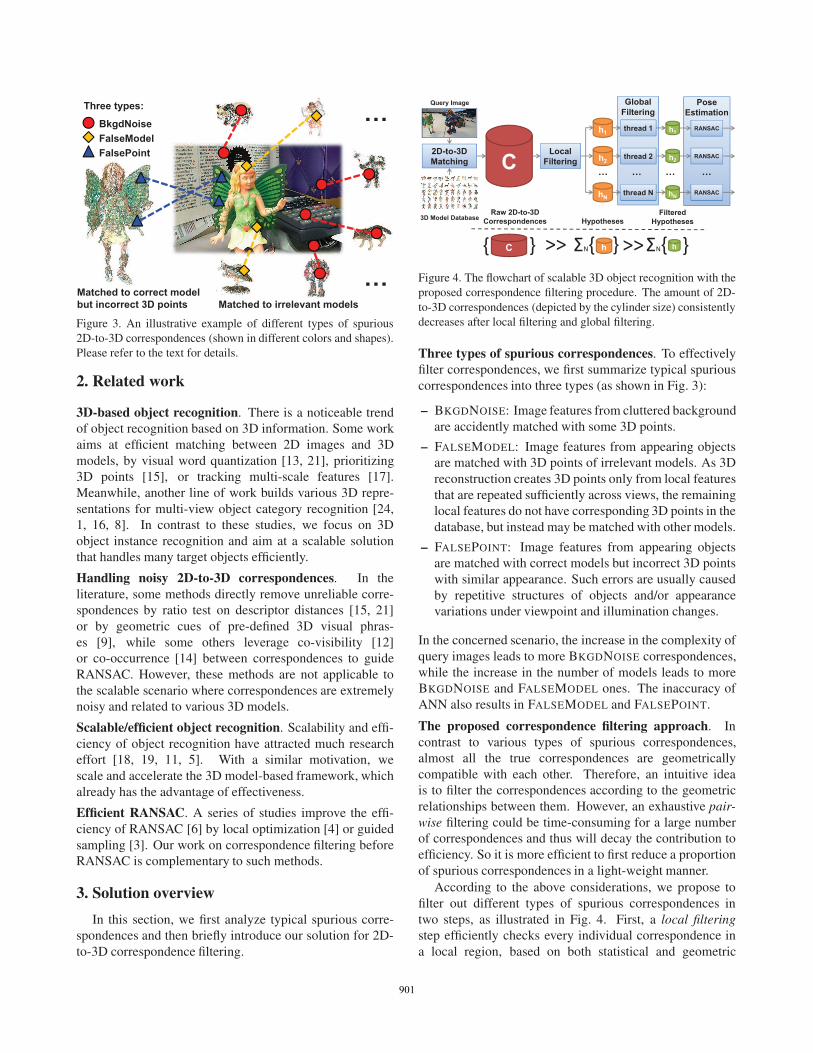
Figure 3. An illustrative example of different types of spurious

2D-to-3D correspondences (shown in different colors and shapes).

Please refer to the text for details.

2. Related work

3D-based object recognition. There is a noticeable trend

of object recognition based on 3D information. Some work

aims at efficient matching between 2D images and 3D

models, by visual word quantization [13, 21], prioritizing

3D points [15], or tracking multi-scale features [17].

Meanwhile, another line of work builds various 3D repre-

sentations for multi-view object category recognition [24,

1, 16, 8]. In contrast to these studies, we focus on 3D

object instance recognition and aim at a scalable solution

that handles many target objects efficiently.

Handling noisy 2D-to-3D correspondences. In the

literature, some methods directly remove unreliable corre-

spondences by ratio test on descriptor distances [15, 21]

or by geometric cues of pre-defined 3D visual phras-

es [9], while some others leverage co-visibility [12]

or co-occurrence [14] between correspondences to guide

RANSAC. However, these methods are not applicable to

the scalable scenario where correspondences are extremely

noisy and related to various 3D models.

Scalable/efficient object recognition. Scalability and effi-

ciency of object recognition have attracted much research

effort [18, 19, 11, 5]. With a similar motivation, we

scale and accelerate the 3D model-based framework, which

already has the advantage of effectiveness.

Efficient RANSAC. A series of studies improve the effi-

ciency of RANSAC [6] by local optimization [4] or guided

sampling [3]. Our work on correspondence filtering before

RANSAC is complementary to such methods.

3. Solution overview

In this section, we first analyze typical spurious corre-

spondences and then briefly introduce our solution for 2D-

to-3D correspondence filtering.

)0�1�1��

2��-��

3��

4��-��

�5

�0

�'

�� 5

�� 0

�� '

�5

�0

�'

-�� 3��

��

%&'(&)

%&'(&)

%&'(&)

*� *��*�� *�

� ��

��

�� %�6�0�1�1��

)��

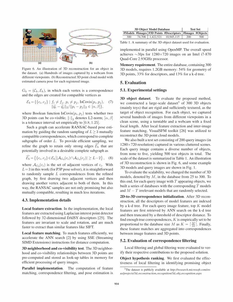
)� �Figure 4. The flowchart of scalable 3D object recognition with the

proposed correspondence filtering procedure. The amount of 2D-

to-3D correspondences (depicted by the cylinder size) consistently

decreases after local filtering and global filtering.

Three types of spurious correspondences. To effectively

filter correspondences, we first summarize typical spurious

correspondences into three types (as shown in Fig. 3):

– BKGDNOISE: Image features from cluttered background

are accidently matched with some 3D points.

– FALSEMODEL: Image features from appearing objects

are matched with 3D points of irrelevant models. As 3D

reconstruction creates 3D points only from local features

that are repeated sufficiently across views, the remaining

local features do not have corresponding 3D points in the

database, but instead may be matched with other models.

– FALSEPOINT: Image features from appearing objects

are matched with correct models but incorrect 3D points

with similar appearance. Such errors are usually caused

by repetitive structures of objects and/or appearance

variations under viewpoint and illumination changes.

In the concerned scenario, the increase in the complexity of

query images leads to more BKGDNOISE correspondences,

while the increase in the number of models leads to more

BKGDNOISE and FALSEMODEL ones. The inaccuracy of

ANN also results in FALSEMODEL and FALSEPOINT.

The proposed correspondence filtering approach. In

contrast to various types of spurious correspondences,

almost all the true correspondences are geometrically

compatible with each other. Therefore, an intuitive idea

is to filter the correspondences according to the geometric

relationships between them. However, an exhaustive pair-

wise filtering could be time-consuming for a large number

of correspondences and thus will decay the contribution to

efficiency. So it is more efficient to first reduce a proportion

of spurious correspondences in a light-weight manner.

According to the above considerations, we propose to

filter out different types of spurious correspondences in

two steps, as illustrated in Fig. 4. First, a local filtering

step efficiently checks every individual correspondence in

a local region, based on both statistical and geometric

899899899901901

cues including spatial consistency and co-visibility. Such

a step has a linear time complexity to the total number

of correspondences, and can remove most of BKGDNOISE

and FALSEMODEL spurious correspondences, which are

generated almost randomly and thus are unlikely to pass

the checks. In this way, local filtering can remove a large

proportion of spurious object hypotheses which have few

valid correspondences left.

To further filter the spurious correspondences that sur-

vive after local filtering, a global filtering step is performed

on each remaining object hypothesis separately to verify

its related correspondences in a pairwise manner. This

step leverages finer-grained 3D geometric cues to evaluate

the compatibility between every two correspondences, and

finally identifies mutually compatible correspondences for

efficient pose estimation. Although the pairwise checks

have a quadratic complexity, the overall computational

cost is well controlled as there are only a few promising

object hypotheses to process, and only a reduced set of

correspondences in each hypothesis.

After such a two-step filtering stage, the remaining

correspondences are much more accurate and are related to

only a few object hypotheses, resulting in a much less effort

of the following pose estimation.

4. Algorithms

We first define some notations as follows. In a 3D

model m, each 3D point p ∈ Pm is a 3D location and is

associated with the scale-invariant local features from a set

Ip of training images in which p has been observed. A 2D-

to-3D correspondence ci is a triplet (fi, pi,mi), indicating

that image feature fi is matched with 3D point pi of object

model mi in the database. In a query image, the whole set

of correspondences is denoted by C =⋃

h∈H Ch, where

H is the set of object hypotheses (i.e., possibly matched

models), and Ch = {ci ∈ C | mi = h} is the subset of

correspondences related to hypothesis h. The algorithms,

integrated with pose estimation, are summarized in Alg. 1.

4.1. Local filtering

Local filtering estimates the confidence of each corre-

spondence by aggregating support from 2D/3D neighbors.

2D local consistency check. From some preliminary

experiments, we observe that image features in true cor-

respondences tend to be close to each other, whereas

image features in BKGDNOISE and FALSEMODEL spurious

correspondences are irregularly distributed. If we treat each

correspondence ci = (fi, pi,mi) as a vote for model mi

at the 2D location of feature fi, true correspondences tend

to reach local consensus whereas spurious ones vote for

inconsistent models irregularly. Therefore, the confidence

of a correspondence can be roughly estimated by checking

Algorithm 1: Correspondence Filtering and Pose Estimation

Input: A set C =⋃

h∈HCh of putative 2D-to-3D correspondences

Output: Camera pose P∗h

for each object hypothesis h ∈ H

begin // Local Filtering

foreach correspondence c ∈ C do

Estimate 2D-3D local support LS2D-3D(c) // Eq. (2)end

foreach hypothesis h ∈ H do

Compute confidence conf(h) from Ch // Eq. (3)end

H ← GetMostConfidentElements(H)

end

foreach hypothesis h ∈ H do

begin // Global Filtering

foreach correspondence c ∈ Ch do

Back-project 2D feature to 3D location // Eq. (6)end

Initialize correspondence graph Gh=(Ch, Eh←∅)Create edges for compatible correspondences // Eq. (7)Refine Gh to retain only strong edges // Eq. (8)

end

begin // Pose Estimation

Initialize optimal camera pose P∗h← 0

for RANSAC iteration r ← 1 to R do

Sample a complete subgraph S={cl}L

l=1from Gh

Solve camera pose Ph from correspondences in Sif Ph better fits Ch than P∗

hthen P∗

h← Ph

end

return P∗h

end

end

its consistency with 2D nearest neighbors. Specifically,

the 2D local support of ci is represented by its 2D nearest

neighbors that correspond to the same model, denoted by

LS2D(ci) = {cj ∈ C | fj ∈ NN 2D(fi), mj = mi} , (1)

where NN 2D(fi) is the set of image features spatially

closest to feature fi, within a circular region of radius that

is proportional to (empirically, 8 times) the scale of fi.

2D-3D local consistency check. 2D local support is useful

for filtering most BKGDNOISE and FALSEMODEL spurious

correspondences. However, there are still a proportion

of such correspondences (e.g., those caused by repetitive

structures in cluttered background) matched accidently

to consistent models and thus survival after 2D local

consistency check. It is therefore necessary to refine the

local support computation by leveraging 3D information.

Since an object appearing in an image is actually a 3D-

to-2D projection of the corresponding 3D point cloud, we

note that if two 3D points pi and pj are close enough in a

3D model, their 2D projections (i.e., image features fi and

fj) from any viewpoint will be very likely to be close; by

contrast, two distant 3D points will be close in 2D space

only from particular viewpoints due to the foreshortening

effect. According to this assumption, we reconsider the

local support from a neighbor correspondence cj to ci, by

900900900902902

further checking whether cj is also a neighbor of ci in 3D

space, leading to a 2D-3D local support set

LS2D-3D(ci) = {cj ∈ LS2D(ci) | pj ∈ NN 3D(pi)} , (2)

where NN 3D(pi) is a subset (i.e., up to 5%) of 3D points

in model mi that are not only spatially closest to pi but also

co-visible with pi from some viewpoints. Here co-visibility

is a crucial constraint because adjacency in 3D Euclidean

space does not necessarily means adjacency in real images.

For instance, it is unlikely to simultaneously observe the

visual patterns on both sides of a coin.

Object hypothesis ranking. As the 2D-3D local support

roughly rates the confidence of each correspondence, it is

straightforward to estimate the confidence of each object

hypothesis h by aggregating the local support of related

correspondences Ch as

conf(h) =∑

ci∈Ch

|LS2D-3D(ci)|, (3)

where |·| is the cardinality of a set. In this way, all the

object hypotheses can be ranked in decreasing order of

confidence, and only the top N are retained for subsequent

processing. Each retained hypothesis is also filtered to

remove correspondences that have no local support.

4.2. Global filtering

After local filtering, putative 2D-to-3D correspondences

are roughly filtered and grouped into a small set of

promising object hypotheses. However, there still might be

spurious correspondences (especially FALSEPOINT ones)

survival, leading to inefficiency in pose estimation. It

is therefore necessary to further filter correspondences

for each hypothesis from a complementary perspective

by checking the 3D geometric compatibility extensively

between correspondences.

Pairwise geometric compatibility check. To efficiently

check whether a set of correspondences are mutually

compatible, i.e., possible to be true simultaneously, it is

desirable to leverage some geometric properties that are

fast to verify and robust to viewpoint changes. In the

literature, some 3D geometric properties (e.g., cross-ratio of

four collinear points [10], cyclic order of three points [9])

are projective-invariant but are defined on at least three 3D

points, leading to high complexity of verification due to

combinatorial explosion.

By contrast, we consider a pairwise geometric property,

i.e., the Euclidean distance between two 3D points, which

is easy to verify and is invariant to 3D coordinate trans-

formations including translation and rotation. Therefore, if

two correspondences ci and cj are compatible, the distance

between 3D points pi and pj in the model coordinate system

should be preserved in the camera coordinate system. For

each correspondence ci, we can estimate pi’s 3D location qi

pi pj

camera coordinate system model coordinate system

image planez = F

cameracenter

y

fi

x

zfj

qi

qj

compatible if|| qi - qj ||2 � || pi - pj ||2

(a)

focal length Fcameracenter

scale(f) size(p)

image plane(b)

z

focal length F

depth D

D / F � size(p) / scale(f)

f

p

Figure 5. An illustration of pairwise geometric compatibility

check. (a) The compatibility between two correspondences is

verified by comparing the inter-point Euclidean distance in model

coordinates and that in camera coordinates (obtained by back-

projecting 2D local features to 3D locations). (b) The correlation

between the size of 3D point p and the scale of 2D local feature f .

in camera coordinates based on the pinhole camera model,

by back-projecting local feature fi in image coordinates

(u(fi), v(fi))�

along the ray passing through the camera

center (as illustrated in Fig. 5 (a)), yielding

qi = (u(fi)·D/F, v(fi)·D/F, D)� , (4)

where F is the known focal length of the query image1, and

D is the depth of qi, the only unknown variable to solve.

Inspired by [7], we assume that each 3D point pi corre-

sponds to a local patch (on the 3D object surface) associated

with an intrinsic absolute size size(pi). Meanwhile, the

observed size of pi in a 2D image, represented by the scale

of local feature fi, is correlated with the depth and focal

length in a pinhole camera model (as shown in Fig. 5 (b)):

D/F ≈ size(pi)/scale(fi). (5)

Combining equations (4) and (5), we obtain an approximate

estimate of qi as

qi =size(pi)

scale(fi)(u(fi), v(fi), F )

�, (6)

where size(pi) = 1

|Ipi|

∑I∈Ipi

scale(fI)DI/FI is pre-

computed by averaging over each training image I ∈ Ipi,

in which pi’s corresponding local feature fI , depth DI , and

image focal length FI are known after 3D reconstruction2.

Graph-based correspondence filtering. For each hypoth-

esis h, we check pairwise compatibility between correspon-

dences in Ch and record the results in an undirected graph

1In this work we use a webcam with a fixed focal length, which is

estimated by calibration. For images captured by modern digital cameras,

focal lengths can usually be obtained from EXIF tags.2This approximate estimation performs well for our current goal.

Explicitly handling point size variation across viewpoints is a future plan.

901901901903903

��

Figure 6. An illustration of 3D reconstruction for an object in

the dataset. (a) Hundreds of images captured by a webcam from

different viewpoints. (b) Reconstructed 3D point cloud model with

estimated camera pose for each registered image.

Gh = (Ch, Eh), in which each vertex is a correspondence

and the edges are created for compatible vertices as

Eh={{ci, cj} | fi �= fj , pi �= pj , IsCovis(pi, pj),‖qi − qj‖2/‖pi − pj‖2 ∈ [α, β]},

(7)

where Boolean function IsCovis(pi, pj) tests whether two

3D points can be co-visible; ‖·‖2

denotes L2-norm; [α, β]is a tolerance interval set empirically to [0.8, 1.25].

Such a graph can accelerate RANSAC-based pose esti-

mation by guiding the random sampling of L≥ 3 mutually

compatible correspondences, which correspond to complete

subgraphs of order L. To provide efficient sampling, we

refine the graph to retain only strong edges Eh that are

potentially involved in a desirable complete subgraph as

Eh={{ci, cj}∈Eh

∣∣|AGh(ci)∩AGh

(cj)| ≥ L−2}, (8)

where AGh(ci) is the set of adjacent vertices of ci. With

L=3 in this work (for P3P pose solver), it is straightforward

to randomly sample L correspondences from the refined

graph, by first drawing two adjacent vertices and then

drawing another vertex adjacent to both of them. In this

way, the RANSAC samples are not only promising but also

mutually compatible, resulting in much less iterations.

4.3. Implementation details

Local feature extraction. In the implementation, the local

features are extracted using Laplacian interest point detector

followed by 32-dimensional DAISY descriptors [25]. The

features are invariant to scale and rotation, and are much

faster to extract than similar features like SIFT.

Local feature matching. To match features efficiently, we

accelerate the ANN search [2] by using SSE (Streaming

SIMD Extensions) instructions for distance computation.

3D neighborhood and co-visibility test. The 3D neighbor-

hood and co-visibility relationships between 3D points are

pre-computed and stored as look-up tables in memory for

efficient processing of query images.

Parallel implementation. The computation of feature

matching, correspondence filtering, and pose estimation is

3D Object Model Database Test Set

#Models #Images #3D Points #Descriptors #Images #Objects

300 74,708 1,422,521 10,945,115 200 500

Table 1. A summary of the 3D object dataset used for evaluation.

implemented in parallel using OpenMP. The overall speed

achieves ∼3fps for 1280×720 images on an Intel i7-870

Quad-Core 2.93GHz processor.

Memory requirement. The entire database, containing 300

3D models, requires 1.2GB memory: 54% for geometry of

3D points, 33% for descriptors, and 13% for a k-d tree.

5. Evaluation

5.1. Experimental settings

3D object dataset. To evaluate the proposed method,

we constructed a large-scale dataset3 of 300 3D objects

(mainly toys) that are rigid and sufficiently textured, as the

target of object recognition. For each object, we captured

several hundreds of images from different viewpoints in a

clean scene, using a turntable and a webcam with a fixed

focal length. After local feature extraction and inter-image

feature matching, VisualSFM toolkit [26] was utilized to

reconstruct the 3D point cloud models.

We also built a test set consisting of 200 query images (in

1280×720 resolution) captured in various cluttered scenes.

Each query image contains a diverse number of objects,

from none to five, yielding 500 test objects in total. The

scale of the dataset is summarized in Table 1. An illustration

of 3D reconstruction is shown in Fig. 6, and some example

3D models and query images are shown in Fig. 1.

To evaluate the scalability, we changed the number of 3D

models, denoted by M , in the database from 25 to 300. To

this end, for each query image with T appearing objects, we

built a series of databases with the corresponding T models

and M − T irrelevant models that are randomly selected.

2D-to-3D correspondence initialization. After 3D recon-

struction, all the descriptors of model features are indexed

by a k-d tree. For each query image feature, top K model

features are first retrieved by ANN search on the k-d tree

and then truncated by a threshold of descriptor distance. To

find enough true correspondences,K is empirically set to be

proportional to the database size M as K = M10. Finally,

these feature matches are aggregated into correspondences

between image features and 3D points.

5.2. Evaluation of correspondence filtering

Local filtering and global filtering were evaluated to ver-

ify their respective contributions to the proposed solution.

Object hypothesis ranking. We first evaluated the effec-

tiveness of local filtering in identifying promising object

3The dataset is publicly available at http://research.microsoft.com/en-

us/projects/3d reconstruction recognition/3d obj recognition.aspx

902902902904904

��

� � � ��

�

�

�

�

��

"

� � ��

+�#

$��

,��

�"��

��

�

�� !��

� - -.0� -.0��

��

��

��

��

��

��

��

� � ��

#$�

��

��

��,�1

��

�

�� !��

� - -.0� -.0��

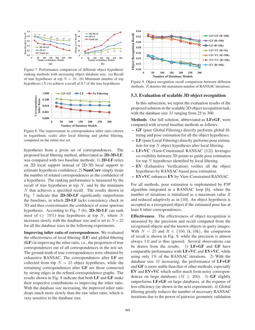
Figure 7. Performance comparison of different object hypothesis

ranking methods with increasing object database size. (a) Recall

of true hypotheses at top N = 10. (b) Minimum number of top

hypotheses (N ) to achieve a recall of 0.7 of the true hypotheses.

��

��

��

��

��

� � ��

��

��

��

��

��

��

��

�� !��

.0230 .0 ��0�� 4

Figure 8. The improvement in correspondence inlier ratio (shown

in logarithmic scale) after local filtering and global filtering,

computed on the entire test set.

hypotheses from a given set of correspondences. The

proposed local filtering method, abbreviated as 2D-3D-LF,

was compared with two baseline methods: 1) 2D-LF relies

on 2D local support instead of 2D-3D local support to

estimate hypothesis confidence; 2) NumCorr simply treats

the number of related correspondences as the confidence of

a hypothesis. The ranking performance is measured by the

recall of true hypotheses at top N , and by the minimum

N that achieves a specified recall. The results shown in

Fig. 7 indicate that 2D-3D-LF significantly outperforms

the baselines, in which 2D-LF lacks consistency check in

3D and thus overestimates the confidence of some spurious

hypotheses. According to Fig. 7 (b), 2D-3D-LF can rank

most of (≥ 70%) true hypotheses at top N , where Nincreases slowly with the database size and is set to N=25for all the database sizes in the following experiments.

Improving inlier ratio of correspondences. We evaluated

the effectiveness of local filtering (LF) and global filtering

(GF) in improving the inlier ratio, i.e., the proportion of true

correspondences out of all correspondences in the test set.

The ground-truth of true correspondences were obtained by

exhaustive RANSAC. The correspondences after LF are

collected from top N = 25 object hypotheses, while the

remaining correspondences after GF are those connected

by strong edges in the refined correspondence graphs. The

results shown in Fig. 8 indicate that both LF and GF make

their respective contributions to improving the inlier ratio.

With the database size increasing, the improved inlier ratio

drops much more slowly than the raw inlier ratio, which is

very sensitive to the database size.

��

��

��

��

��

��

��

��

� � ��

5�6

��

��4

��

��

��

�

�� !��

.0230�7�'��8

30�7�'��8

.0�7�'��98

.02&��7�'�98

.02&��7�'��98

:&2&��7�'��98

:&�7�'��98

Figure 9. Object recognition recall comparison between different

methods. R denotes the maximum number of RANSAC iterations.

5.3. Evaluation of scalable 3D object recognition

In this subsection, we report the evaluation results of the

proposed solution in the scalable 3D object recognition task,

with the database size M ranging from 25 to 300.

Methods. Our full solution, abbreviated as LF+GF, were

compared with several baseline methods as follows:

– GF (pure Global Filtering) directly performs global fil-

tering and pose estimation for all the object hypotheses.

– LF (pure Local Filtering) directly performs pose estima-

tion for top N object hypotheses after local filtering.

– LF+VC (View-Constrained RANSAC [12]) leverages

co-visibility between 3D points to guide pose estimation

for top N hypotheses identified by local filtering.

– EV (Exhaustive Verification) verifies all the object

hypotheses by RANSAC-based pose estimation.

– EV+VC enhances EV by View-Constrained RANSAC.

For all methods, pose estimation is implemented by P3P

algorithm integrated in a RANSAC loop [6], where the

number of iterations is initialized as a maximum value Rand reduced adaptively as in [10]. An object hypothesis is

accepted as a recognized object if the estimated pose has at

least 8 inlier correspondences.

Effectiveness. The effectiveness of object recognition is

measured by the precision and recall computed from the

recognized objects and the known objects in query images.

With N = 25 and R ∈ {100, 1k, 10k}, the comparison

of recall is shown in Fig. 9, while the precision is almost

always 1.0 and is thus ignored. Several observations can

be drawn from the results. 1) LF+GF and GF have

comparable performance with LF+VC and EV+VC, while

using only 1% of the RANSAC iterations. 2) With the

database size M increasing, the performance of LF+GF

and GF is more stable than that of other methods, especially

EV and EV+VC which suffer much from noisy correspon-

dences on large databases (M ≥ 200). 3) GF slightly

outperforms LF+GF on large databases, at the expense of

less efficiency (as shown in the next experiment). 4) Global

filtering greatly reduces the number of necessary RANSAC

iterations due to the power of pairwise geometric validation

903903903905905

1.0E+01

1.0E+02

1.0E+03

1.0E+04

1.0E+05

0 50 100 150 200 250 300Com

puta

tiona

l Cos

t (m

s)

Number of Database Models

LF+GF (R=100)

GF (R=100)

LF+VC (R=10k)

EV+VC (R=10k)

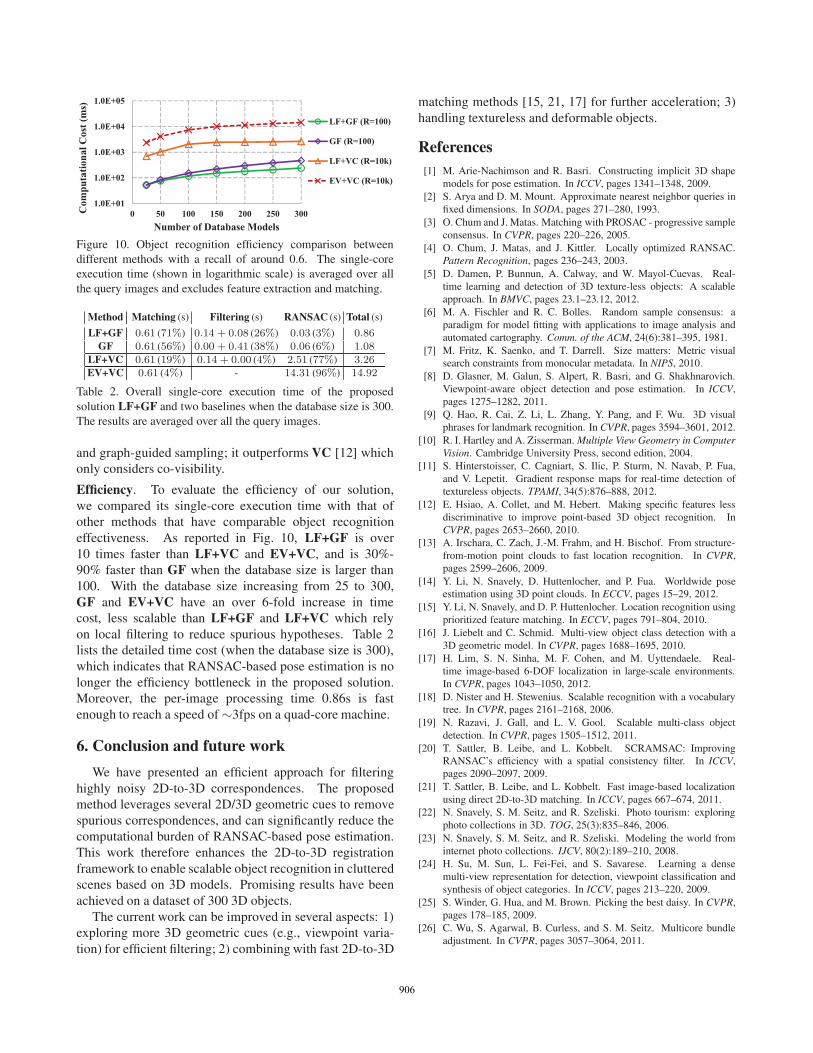
Figure 10. Object recognition efficiency comparison between

different methods with a recall of around 0.6. The single-core

execution time (shown in logarithmic scale) is averaged over all

the query images and excludes feature extraction and matching.

Method Matching (s) Filtering (s) RANSAC (s) Total (s)

LF+GF 0.61 (71%) 0.14 + 0.08 (26%) 0.03 (3%) 0.86GF 0.61 (56%) 0.00 + 0.41 (38%) 0.06 (6%) 1.08

LF+VC 0.61 (19%) 0.14 + 0.00 (4%) 2.51 (77%) 3.26EV+VC 0.61 (4%) - 14.31 (96%) 14.92

Table 2. Overall single-core execution time of the proposed

solution LF+GF and two baselines when the database size is 300.

The results are averaged over all the query images.

and graph-guided sampling; it outperforms VC [12] which

only considers co-visibility.

Efficiency. To evaluate the efficiency of our solution,

we compared its single-core execution time with that of

other methods that have comparable object recognition

effectiveness. As reported in Fig. 10, LF+GF is over

10 times faster than LF+VC and EV+VC, and is 30%-

90% faster than GF when the database size is larger than

100. With the database size increasing from 25 to 300,

GF and EV+VC have an over 6-fold increase in time

cost, less scalable than LF+GF and LF+VC which rely

on local filtering to reduce spurious hypotheses. Table 2

lists the detailed time cost (when the database size is 300),

which indicates that RANSAC-based pose estimation is no

longer the efficiency bottleneck in the proposed solution.

Moreover, the per-image processing time 0.86s is fast

enough to reach a speed of ∼3fps on a quad-core machine.

6. Conclusion and future work

We have presented an efficient approach for filtering

highly noisy 2D-to-3D correspondences. The proposed

method leverages several 2D/3D geometric cues to remove

spurious correspondences, and can significantly reduce the

computational burden of RANSAC-based pose estimation.

This work therefore enhances the 2D-to-3D registration

framework to enable scalable object recognition in cluttered

scenes based on 3D models. Promising results have been

achieved on a dataset of 300 3D objects.

The current work can be improved in several aspects: 1)

exploring more 3D geometric cues (e.g., viewpoint varia-

tion) for efficient filtering; 2) combining with fast 2D-to-3D

matching methods [15, 21, 17] for further acceleration; 3)

handling textureless and deformable objects.

References

[1] M. Arie-Nachimson and R. Basri. Constructing implicit 3D shape

models for pose estimation. In ICCV, pages 1341–1348, 2009.

[2] S. Arya and D. M. Mount. Approximate nearest neighbor queries in

fixed dimensions. In SODA, pages 271–280, 1993.

[3] O. Chum and J. Matas. Matching with PROSAC - progressive sample

consensus. In CVPR, pages 220–226, 2005.

[4] O. Chum, J. Matas, and J. Kittler. Locally optimized RANSAC.

Pattern Recognition, pages 236–243, 2003.

[5] D. Damen, P. Bunnun, A. Calway, and W. Mayol-Cuevas. Real-

time learning and detection of 3D texture-less objects: A scalable

approach. In BMVC, pages 23.1–23.12, 2012.

[6] M. A. Fischler and R. C. Bolles. Random sample consensus: a

paradigm for model fitting with applications to image analysis and

automated cartography. Comm. of the ACM, 24(6):381–395, 1981.

[7] M. Fritz, K. Saenko, and T. Darrell. Size matters: Metric visual

search constraints from monocular metadata. In NIPS, 2010.

[8] D. Glasner, M. Galun, S. Alpert, R. Basri, and G. Shakhnarovich.

Viewpoint-aware object detection and pose estimation. In ICCV,

pages 1275–1282, 2011.

[9] Q. Hao, R. Cai, Z. Li, L. Zhang, Y. Pang, and F. Wu. 3D visual

phrases for landmark recognition. In CVPR, pages 3594–3601, 2012.

[10] R. I. Hartley and A. Zisserman. Multiple View Geometry in Computer

Vision. Cambridge University Press, second edition, 2004.

[11] S. Hinterstoisser, C. Cagniart, S. Ilic, P. Sturm, N. Navab, P. Fua,

and V. Lepetit. Gradient response maps for real-time detection of

textureless objects. TPAMI, 34(5):876–888, 2012.

[12] E. Hsiao, A. Collet, and M. Hebert. Making specific features less

discriminative to improve point-based 3D object recognition. In

CVPR, pages 2653–2660, 2010.

[13] A. Irschara, C. Zach, J.-M. Frahm, and H. Bischof. From structure-

from-motion point clouds to fast location recognition. In CVPR,

pages 2599–2606, 2009.

[14] Y. Li, N. Snavely, D. Huttenlocher, and P. Fua. Worldwide pose

estimation using 3D point clouds. In ECCV, pages 15–29, 2012.

[15] Y. Li, N. Snavely, and D. P. Huttenlocher. Location recognition using

prioritized feature matching. In ECCV, pages 791–804, 2010.

[16] J. Liebelt and C. Schmid. Multi-view object class detection with a

3D geometric model. In CVPR, pages 1688–1695, 2010.

[17] H. Lim, S. N. Sinha, M. F. Cohen, and M. Uyttendaele. Real-

time image-based 6-DOF localization in large-scale environments.

In CVPR, pages 1043–1050, 2012.

[18] D. Nister and H. Stewenius. Scalable recognition with a vocabulary

tree. In CVPR, pages 2161–2168, 2006.

[19] N. Razavi, J. Gall, and L. V. Gool. Scalable multi-class object

detection. In CVPR, pages 1505–1512, 2011.

[20] T. Sattler, B. Leibe, and L. Kobbelt. SCRAMSAC: Improving

RANSAC’s efficiency with a spatial consistency filter. In ICCV,

pages 2090–2097, 2009.

[21] T. Sattler, B. Leibe, and L. Kobbelt. Fast image-based localization

using direct 2D-to-3D matching. In ICCV, pages 667–674, 2011.

[22] N. Snavely, S. M. Seitz, and R. Szeliski. Photo tourism: exploring

photo collections in 3D. TOG, 25(3):835–846, 2006.

[23] N. Snavely, S. M. Seitz, and R. Szeliski. Modeling the world from

internet photo collections. IJCV, 80(2):189–210, 2008.

[24] H. Su, M. Sun, L. Fei-Fei, and S. Savarese. Learning a dense

multi-view representation for detection, viewpoint classification and

synthesis of object categories. In ICCV, pages 213–220, 2009.

[25] S. Winder, G. Hua, and M. Brown. Picking the best daisy. In CVPR,

pages 178–185, 2009.

[26] C. Wu, S. Agarwal, B. Curless, and S. M. Seitz. Multicore bundle

adjustment. In CVPR, pages 3057–3064, 2011.

904904904906906

efficient 2d-to-3d correspondence filtering for scalable ... · efﬁcient 2d-to-3d correspondence...

Documents