Full Title: THE WEAK-FORM EFFICIENCY OF CHINESE STOCK MARKETS: THIN TRADING, NONLINEARITY AND EPISODIC SERIAL DEPENDENCIES

Authors: Kian-Ping Lima, b*, Muzafar Shah Habibullahc and Melvin J. Hinichd Affiliations: a Labuan School of International Business and Finance Universiti Malaysia Sabah

b Department of Econometrics and Business Statistics Monash University c Department of Economics Faculty of Economics and Management Universiti Putra Malaysia d Applied Research Laboratories

University of Texas at Austin

Abstract: Motivated by the shortcomings of earlier Chinese efficiency studies, the present paper re-examines the weak-form efficiency of Shanghai and Shenzhen Stock Exchanges. Specifically, our adopted methodologies mitigate the confounding effect of thin trading on autocorrelation, detect both linear and nonlinear serial dependencies in the adjusted returns series, and capture the persistence of dependency structures over time. The result shows that the adjusted returns series from both markets follow a random walk for long periods of time, only to be interspersed with brief periods of strong linear and/or nonlinear dependency structures. This suggests that there are certain time periods when new information is not fully reflected into stock prices. Another interesting finding is that the existence of serial dependencies in both the Shanghai and Shenzhen Stock Exchanges follows one another closely after October 1997. It indicates that both markets responded in a similar way to influences from political, economic, social and institutional changes.

JEL Classifications: G14; G15; C49. Keywords: Nonlinearity; Thin trading; Market efficiency; China; Stock market.

* Corresponding author. Department of Econometrics and Business Statistics, Monash University, Building H, Level 5, 900 Dandenong Road, P.O. Box 197, Caulfield East, Victoria 3145, Australia. Phone: 61-3-99034531; Fax: 61-3-99032007; Email: KianPing.Lim@buseco.monash.edu.au.

2

1. Introduction

In recent years, China has been in the limelight following her spectacular economic growth

since the adoption of market-oriented reforms in 1978, with real GDP growth averaging 9.5%

per annum for the period 1979-2003. With her admission into the World Trade Organization

(WTO) in December 2001, the development of the two stock markets located in Shanghai

and Shenzhen will be watched even more closely by academics, investors and policy makers.

Though both the Shanghai Stock Exchange (SHSE) and Shenzhen Stock Exchange (SZSE)

are relatively young with their respective inauguration in December 1990 and July 1991, they

are the world’s leading emerging stock market in terms of market capitalization, and Asia’s

second largest after Japan. By the end of September 2004, the number of listed companies on

both exchanges stood at 1378, with a combined market capitalization of 4.093 trillion

Renminbi (approximately US$495 billion), more than 70 million stock traders, and a trading

volume that hit 62.65 billion shares in the month of September 2004.1

The Chinese markets exhibit some unique ‘Chinese characteristics’ not found in other stock

markets. This has prompted researchers to investigate various aspects of the stock markets

since no generalization can be made and to some extent no reference point exists. First, the

ownership structure of a listed company can be classified into as many as five different

classes: state-owned shares, legal-person shares, employee shares, tradable A-shares and

shares only available to foreign investors. The distinguishing characteristic is that over 60%

of the total equities of listed companies are non-negotiable shares (state-owned shares, legal-

person shares and employee shares) that cannot be traded on the exchanges (Qi et al., 2000;

Wei and Varela, 2003). Second, the tradable A- and B-shares markets are characterized by

1 Data source: China Securities Regulatory Commission (CSRC), at http://www.csrc.gov.cn/. At the end of September 2004, the exchange rate was 8.27 Renminbi per U.S. dollar.

3

the dominance of individual investors with Chinese institutional investors such as the pension

funds, insurance companies and securities companies accounting for less than 10% of the

total market capitalization.2 It is widely acknowledged that these individual investors trade

like noise traders, subject to herd behaviour and treat the market like a casino without

considering the information or fundamentals related to firms (Ma, 1996; Nam et al., 1999;

Kang et al., 2002; Girardin and Liu, 2003).3 Third, though both the A- and B-shares have

identical ownership rights and dividends within the same company, the latter are traded at

substantial discounts relative to the former, suggesting that Chinese investors pay higher

prices for identical shares than their foreign counterparts (Bailey, 1994; Ma, 1996; Sun and

Tong, 2000; Gordon and Li, 2003). This is indeed a big puzzle as shares traded on other

Asian and European stock markets are sold at considerable premiums to foreigners (for

specific examples, refer to Bailey et al., 1999). Fourth, the volatility of domestic A-shares is

much higher than those of foreign B-shares, despite both are seemingly similar assets (Su and

Fleisher, 1999b; He et al., 2003). Fifth, though the phenomenon of initial public offering

(IPO) underpricing is documented in other stock markets (for specific examples, see Mok and

Hui, 1998: 454), the degree of IPO underpricing in Chinese A-shares market is extremely

large (Mok and Hui, 1998; Su and Fleisher, 1999a; Chen et al., 2004).

In addition to the aforementioned aspects, the efficiency of the Chinese stock markets is not

exempted from the strict scrutiny of researchers in views of its profound significance to

market regulators and investors. In general, the focus of extant literature is on the weak-form

2 In 2003, the Shanghai Stock Exchange has a total of 36,436,000 investor accounts, of which 35,266,000 are A-shares accounts, 980,600 are B-shares accounts and 189,400 institutional investors (Shanghai Stock Exchange Fact Book 2003, downloaded from http://www.sse.com.cn/sseportal/en_us/ps/about/fact.shtml). For Shenzhen Stock Exchange, total individual investors in 2003 are 33,632,231, of which 33,040,600 are in A-shares market with the remaining 591,631 in B-shares market. Institutional investors, on the other hand, account for only 0.5%, with a mere figure of 182,523 (Shenzhen Stock Exchange Fact Book 2003, downloaded from http://www.szse.cn/main/en/MarketStatistics/FactBook/). For reasons behind the dominance of individual investors, refer to Kang et al. (2002: Footnote 7). 3 Nam et al. (1999: 79) provided some explanations for the speculative behaviour of these individual investors.

4

version of the efficient markets hypothesis (EMH), which asserts that stock prices fully

reflect all information contained in the past price history of the market. The empirical

investigations revolved around examining whether stock prices follow a random walk process

(Laurence et al., 1997; Liu et al., 1997; Long et al., 1999; Mookerjee and Yu, 1999; Darrat

and Zhong, 2000; Lee et al., 2001; Groenewold et al., 2003, 2004; Lima and Tabak, 2004;

Ma, 2004; Seddighi and Nian, 2004). Taken as a whole, no consensus could be reached on

the weak-form efficiency of these Chinese stock markets. On one hand, Liu et al. (1997),

Laurence et al. (1997), Long et al. (1999) and Lima and Tabak (2004) concluded that the

Chinese markets are efficient as their respective stock returns do not exhibit predictable

patterns. On the other end of the spectrum, Mookerjee and Yu (1999) and Ma (2004)

proclaimed the markets as inefficient given that the random walk hypothesis is rejected by

their efficiency tests. In between are those studies that found evidence of returns

predictability, yet avoided making inference on market inefficiency as these authors were

mindful that the detected predictability could be spurious autocorrelation induced by thin

trading.

However, the above-cited Chinese efficiency studies assumed deviation from a random walk

is in the form of linear serial correlations, and market efficiency is a static characteristic that

remains unchanged over the entire estimation period. Their shortcomings are further

discussed in Section 2. Section 3 then outlines our proposed research framework to address

the problem of thin trading, the possibility of nonlinearity in the data generating process, and

the persistency of serial dependencies over time. Following that, descriptions of the data and

methodologies are provided. Section 5 presents the empirical results and provides plausible

explanations for the contradicting empirical evidence in earlier Chinese efficiency studies.

The final section then concludes the paper.

5

2. The Weak-form Efficiency of Chinese Stock Markets: Literature Review

The present section contains a review of previous studies that addressed the weak-form

efficiency of Chinese stock markets. Our discussions highlight their major shortcomings, in

particularly the robustness of results and methodologies employed.

Firstly, the efficiency findings reported by various authors (Liu et al., 1997 for both SHSE

and SZSE; Laurence et al., 1997 and Lima and Tabak, 2004 for A-shares markets in both

SHSE and SZSE; Long et al., 1999 for A- and B-shares markets in SHSE) are quite

surprising given the widely-shared perception that these Chinese stock markets are highly

speculative, driven mainly by market rumours and individual investor sentiment. On one

hand, the trading of noise traders would lead to serially correlated stock returns. For instance,

the theoretical model of De Long et al. (1990) showed that when noise traders follow a

positive feedback trading strategy, the price pressure induces positive return autocorrelation

at short horizons. On the other hand, their evidence is inconsistent with studies that examined

the profitability of past-return based investment strategies in the Chinese markets. For

instance, Kang et al. (2002) reported statistically significant abnormal profits for some short-

horizon contrarian and intermediate-horizon momentum strategies in the A-shares market.

Based on 412 technical trading rules, Tian et al. (2002) found that these rules are quite

successful in predicting the stock price movements in both Chinese stock exchanges,

allowing traders to make possible excess profits during the 1990s.

Secondly, though all the aforementioned Chinese studies employed the conventional and

popular efficiency tests, they are not without defect. Laurence et al. (1997) and Mookerjee

and Yu (1999) drew their conclusions based solely on the results of serial correlation and

runs tests. Liu et al. (1997) only employed unit root tests to examine the random walk

6

hypothesis, while the analyses in Groenewold et al. (2003, 2004) and Seddighi and Nian

(2004) were conducted using autocorrelation and unit root tests. However, the Monte Carlo

experiments performed by Lo and Mackinlay (1989) demonstrated that the above statistical

tests are less powerful relative to the variance ratio tests in detecting serial correlations of

stock returns. Moreover, Campbell et al. (1997) argued that the detection of a unit root cannot

be used as a basis to support the random walk hypothesis, hence the efficiency of the

underlying stock market since unit root tests are not designed to test for predictability of

stock prices.4 As a result, many researchers either complemented or relied on variance ratio

tests in their empirical testing of the random walk hypothesis (Long et al., 1999; Darrat and

Zhong, 2000; Lee et al., 2001; Lima and Tabak, 2004; Ma, 2004). Unfortunately, as noted by

Antoniou et al. (1997a, b), emerging stock markets like China are typically characterized by

thin trading and this would introduce bias into the above autocorrelation-based tests of

market efficiency. Specifically, it is well established in the literature that this institutional

feature would induce spurious autocorrelation in stock returns that is not genuine

predictability, but rather a statistical illusion (see, for example, Lo and MacKinlay, 1988,

1990; Miller et al., 1994). Surprisingly, no attempt has been made by these earlier studies to

remove the impact of thin trading, though some of them did acknowledge that thin trading

could be the culprit for the detected predictability in their studies (Laurence et al., 1997;

Groenewold et al., 2003, 2004).

4 Darrat and Zhong (2000) and Li (2003b) also questioned the use of unit root tests by earlier studies to examine the efficiency of Chinese stock markets. For recent critiques on the application of unit root tests, see Saadi et al. (2006a, b) and Rahman and Saadi (2007, 2008).

7

Thirdly, another common institutional feature that these Chinese efficiency studies have

neglected is the possible existence of nonlinear serial dependence in stock returns series

(Antoniou et al., 1997a; Appiah-Kusi and Menyah, 2003).5 Empirically, after it was first

reported by Hinich and Patterson (1985), more and more evidence has emerged to suggest

nonlinear dependence in stock returns is a universal phenomenon (see references cited in Lim

et al., 2006). In fact, based on the success of the artificial neural network model in forecasting

Chinese stock prices, Darrat and Zhong (2000) acknowledged that prices may be better

captured by nonlinear processes. The possible existence of nonlinear dependence in stock

returns has important implication on the validity of weak-form EMH as it suggests the

potential of returns predictability. Brooks and Hinich (1999) argued that if nonlinearity is

present in the conditional first moment, it may be possible to devise a trading strategy based

on nonlinear model which is able to yield higher returns than a buy-and-hold rule. Neftci

(1991) demonstrated that in order for technical trading rules to be successful, some form of

nonlinearity in stock prices is necessary. In testing the primary hypothesis that graphical

technical analysis methods may be equivalent to nonlinear forecasting methods, Clyde and

Osler (1997) found that technical analysis works better on nonlinear data than on random

data, and the use of technical analysis can generate higher profits than a random trading

strategy if the data generating process is nonlinear. Indeed, there are a number of studies that

documented the profitability of nonlinear trading rules (see, for example, Gençay, 1998;

Fernández-Rodríguez et al., 2000; Andrada-Félix et al., 2003).

It is worth highlighting that the statistical tests adopted in earlier Chinese efficiency studies

are not capable of detecting nonlinearity since they are all designed to uncover linear

relationships between the returns and their past values. However, the lack of linear

5 For factors that might induce nonlinear dependence in stock returns series, interested readers can consult Antoniou et al. (1997a), Sarantis (2001) and Lim et al. (2006).

8

correlations does not necessarily imply efficiency as returns series can be linearly

uncorrelated and at the same time nonlinearly dependent. This piece of advice has been given

to researchers almost three decades ago by Granger and Andersen (1978), and then follow-up

by Granger (1983) in his appropriately titled ‘Forecasting white noise’. Specifically, the latter

demonstrated that one can never be sure time series with zero autocorrelation is not

forecastable. In fact, it is well-known now time series generated by bilinear and nonlinear

moving average processes exhibit zero autocorrelation yet possess predictable nonlinearities

in mean. Hence, even if the returns series appear ‘random’ to autocorrelation-based tests, it

still leaves wide open the question of whether higher-order temporal correlations exist. Until

and unless this has been diagnosed, no convincing conclusion for independence of price

changes can be offered. Motivated by the above concern, a number of studies have

questioned the validity of inferences on market efficiency drawn from autocorrelation-based

tests, and proceeded to conduct a re-examination using statistical tools that are designed to

account for nonlinear dependence (see, for example, Al-Loughani and Chappell, 1997;

Antoniou et al., 1997a; Blasco et al., 1997; Freund et al., 1997; Kohers et al., 1997; Chappel

et al., 1998; Opong et al., 1999; Freund and Pagano, 2000; Hamill et al., 2000; Poshakwale,

2002; Appiah-Kusi and Menyah, 2003; Hassan et al., 2003; Narayan, 2005; Panagiotidis,

2005).

Finally, all these Chinese studies focused on the all-or-nothing notion of absolute market

efficiency, handing down the verdict of whether a market is or is not weak-form efficient for

the whole sample period under study. However, it is unreasonable to expect the market to be

efficient all the time. Self and Mathur (2006: 3154) wrote: “The true underlying market

structure of asset prices is still unknown. However, we do know that, for a period of time, it

behaves according to the classical definition of an efficient market; then, for a period, it

9

behaves in such a way that researchers are able to systematically find anomalies to the

behavior expected of an efficient market”. On the other hand, Emerson et al. (1997) argued

that it is not sensible to address the issue of market efficiency/inefficiency for stock markets

in Central and Eastern European transition economies that have just emerged out of the

former communist bloc such as Bulgaria and Hungary. The main reason is that when a

market first opens, it is hardly credible for the market to be efficient since it takes time for the

price discovery process to become known. However, as markets operate and market

microstructures develop, within a finite amount of time, they are likely to become more

efficient. Hence, the more relevant research question is whether and how these infant markets

are becoming more efficient, and this certainly cannot be answered by classical steady-

variable approaches that assume a fixed level of market efficiency throughout the entire

estimation period. On a theoretical ground, the adaptive markets hypothesis (AMH) of Lo

(2004, 2005) hypothesized that market efficiency is not an all-or-none condition but is a

characteristic that varies continuously over time and across markets, which is likely the result

of institutional changes in the stock markets as well as the entry and exit of various market

participants.

In extant literature, Emerson et al. (1997) proposed a time-varying parameter model to

capture the changing degree of market efficiency over time. In their proposed framework, the

time-varying autoregressive coefficients are used to gauge the changing degree of

predictability, and hence evolving weak-form market efficiency. If the market under study

becomes more efficient over time, the smoothed time-varying estimates of the autocorrelation

coefficient would gradually converge towards zero and become insignificant. The framework,

formalized by Zalewska-Mitura and Hall (1999) as “Test for Evolving Efficiency”, was

subsequently adopted to assess the evolution of efficiency for stock markets in Central and

10

Eastern European transition economies (Zalewska-Mitura and Hall, 2000; Rockinger and

Urga, 2000, 2001), China (Li, 2003a, b), Africa (Jefferis and Smith, 2004, 2005), and Jordan

(Maghyereh, 2005). Though the time-varying framework proposed by Emerson et al. (1997)

has relaxed the assumption of static equilibrium, the focus is still limited to linear

correlations. In this regard, the statistical inferences drawn from Li (2003a, b) for the Chinese

stock markets should be met with scepticism. On one hand, the evidence of significant

autocorrelation coefficients during certain time periods could be spurious autocorrelation

induced by thin trading and led to incorrect verdict on market inefficiency, since no

adjustment procedure was adopted by the author to purge the thin trading effect. For instance,

Li (2003a) attributed the high predictability reported for both Shanghai and Shenzhen stock

returns during the earlier stages of development to market inefficiency as well as market

illiquidity. On the other hand, for those periods with no evidence of linear predictability, the

possibility that the underlying returns series are nonlinearly dependent could not be ruled out.

3. An Overview of the Research Framework

It is clear then from our literature review that predictability is assumed by earlier Chinese

efficiency studies to take the form of linear correlations, and market efficiency is a static

characteristic that remains unchanged over the entire estimation period. However, with the

availability of advanced statistical tests, these two assumptions have been found to be

inappropriate. Methodologically, in examining the efficiency of stock market, the research

framework adopted should: (1) mitigate the confounding effect of thin trading on

autocorrelation; (2) detect both linear and nonlinear serial dependencies; (3) capture the

persistence of deviation from a random walk over time.

11

While adjustment procedures to correct for spurious autocorrelation due to thin trading are

available in existing literature, they were only adopted by a handful of efficiency studies

(Antoniou et al., 1997a, b; Abraham et al., 2002; Appiah-Kusi and Menyah, 2003; Hassan et

al., 2003; Al-Khazali et al., 2007; Rayhorn et al., 2007). The methodology adopted in this

paper to deal with the problem of thin trading was proposed by Miller et al. (1994). Briefly,

the analysis in Miller et al. (1994) demonstrated that the observed price changes can be

adjusted by (1- ϕ ) to remove the impact of thin trading in the calculation of returns, where

the parameter ϕ measures the degree of trading infrequency. In applying their model to index

returns, a moving average (MA) model where the number of moving average components is

equal to the number of non-trading days should be estimated (Miller et al., 1994: 507-510).

However, given the difficulties in identifying the non-trading days, the authors showed that it

is equivalent to estimating an autoregressive (AR) model of order one, and the residuals from

such a model are scaled up by (1- ϕ ) to remove the impact of thin trading in the returns

calculation.

To detect both linear and nonlinear serial dependencies in the returns series, we employ two

test statistics proposed by Hinich and Patterson (1995, 2005). The first one is a portmanteau

correlation test statistic, denoted as the C statistic, which is a modified version of the Box-

Pierce Q-statistic. Unlike the Q-statistic that is usually applied to the residuals of a fitted

autoregressive moving average (ARMA) model, the C statistic is a function of the

standardized observations and the number of lags used depends on the sample size. Despite

these differences, both the Q and C statistics perform the same function, that is, to detect the

presence of linear dependence in the form of significant autocorrelations or known as second-

order correlations. The second test statistic is the portmanteau bicorrelation test statistic

denoted as the H statistic, which is a third-order extension of the standard correlation test for

12

white noise. The orientation for this test is based on the premise that the bicorrelations should

all be equal to zero if a time series is generated by a linear Gaussian process. Conversely, if a

process generating a time series has non-zero bicorrelations, then the process is nonlinear.

Hence, the portmanteau bicorrelation test relies on the zero bicorrelation property of linear

process to test for the presence of nonlinear serial dependence, and the H statistic is able to

pick up many types of nonlinearity in the conditional mean that generate third-order

nonlinear dependence. On the other hand, this nonlinearity test is the preferred choice for two

reasons. First, it has good small-sample properties (Hinich and Patterson, 1995, 2005; Hinich,

1996). Second, the test suggests an appropriate functional form for a nonlinear forecasting

equation. In particular, Brooks and Hinich (2001) demonstrated via their proposed univariate

bicorrelation forecasting model that the bicorrelations can be used to forecast the future

values of the series under consideration. Given the possibility that serial dependencies, linear

and nonlinear, detected in the full sample could actually be triggered by those strong

significant results in a few small sub-periods, both the C and H statistics are computed in

non-overlapped moving sub-samples or known as time windows.

4. The Stock Market Data and Methodologies

4.1 Data description

In China, a local firm can issue two different classes of shares to be traded on SHSE or SZSE,

but cross-listing of shares at the two official exchanges is not permitted.6 The A-shares,

denominated and traded in Chinese currency, are restricted to domestic investors. On the

other hand, the B-shares, also denominated in Renminbi, are traded in foreign currency (U.S.

6 Chinese firms with approval from the government may list their shares on foreign stock exchanges as H-shares. At the end of September 2004, there are 104 H-shares traded in the U.S., U.K., Singapore and Hong Kong, with Hong Kong Stock Exchange the preferred venue. Of these, 29 firms have A-shares counterparts listed on the Chinese domestic stock exchanges.

13

dollars in Shanghai and Hong Kong dollars in Shenzhen) and restricted to foreign investors.

However, the Chinese government has gradually relaxed the share tradability restriction.

Since 28 February 2001, local investors with foreign currency accounts are allowed to trade

the B-shares, while trading of A-shares is opened to international institutional investors in

December 2002 under the Qualified Foreign Institutional Investor (QFII) scheme. According

to China Securities Regulatory Commission (CSRC), of the 1378 listed companies on both

stock exchanges as at September 2004, only 1238 listed companies offer A-shares, while 24

firms issue B-shares only. There are 86 firms that issue both A- and B-shares to domestic and

foreign investors respectively. In terms of market capitalization and the level of activity, A-

shares dominated the Chinese stock markets, and B-shares have been illiquid and less active

since inception.

The data in this study consist of daily closing prices for Shanghai SE Composite Price Index

and Shenzhen SE Composite Price Index, covering the sample period from the earliest

available date in Datastream database (Shanghai- January 2, 1991; and Shenzhen- April 3,

1991) to 12/31/2003. These indices are price-weighted series of all listed stocks on the two

exchanges, excluding dividends. The base value of the Shanghai SE Composite Price Index is

100 points in December 1990 while the base date for Shenzhen SE Composite Price Index is

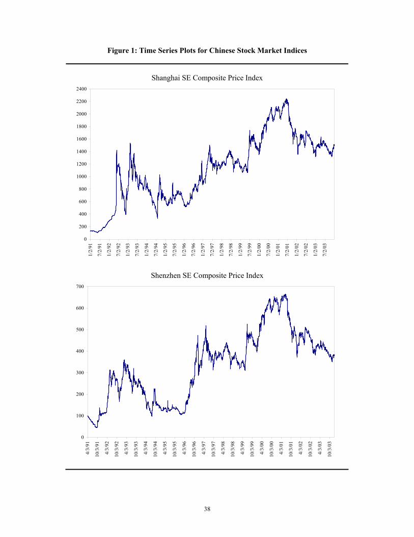
April 1991. The time series plots in Figure 1 illustrate the evolution of these two Chinese

stock market indices over the selected sample period. In our empirical analyses, the index

data are transformed into a series of continuously compounded percentage returns,

( ),ln*100 1−= ttt ppR where tp is the closing price of the index on day ,t and 1tp − the price

on the previous trading day.

14

<<Insert Figure 1 about here>>

A close inspection of Figure 1 reveals that the two time series plots are mirror reflection of

each another, indicating that the Shanghai SE Composite Price Index moved hand-in-hand

with its Shenzhen counterpart. Even more striking is that the peaks and troughs in both

indices occurred around the same time. It could be that their movements were driven by the

same underlying factors, as discussed in great detail by Groenewold et al. (2004: 9-25).

Several notable accounts are quoted and presented here: (1) The double-digits economic

growth and high inflation rate in year 1992 have boosted trading in the two Chinese stock

exchanges. The Shanghai SE Composite Price Index peaked at 1536.82 on 15 February 1993,

while the Shenzhen SE Composite Price Index reached its peak of 359.44 on 22 February

1993, as compared to their base values of 100 in December 1990 and April 1991 respectively;

(2) Prior to 1994, the state banks were dominant in share trading. However, banks were

required to quit their direct involvement in the stock markets in 1994. Consequently, bank

stock-broking departments and subsidiaries became independent broker houses. The

withdrawal of large sums of funds by the state banks from both stock exchanges and the

government’s anti-inflation measures led directly to the share market stagnation between

early 1994 to April 1996. During this period, the composite indices in both exchanges

reached their respective troughs on 29 July 1994, with Shanghai SE Composite Price Index

bottomed at 333.92 and Shenzhen SE Composite Price Index fell to 96.56; (3) From April

1996, the two Chinese stock exchanges enjoyed a strong rally, only to be halted by the “Black

Monday” on 16 December 1996 due to the disclosure of illicit speculation by the Shenzhen

15

Development Bank. The government took strict measures to punish the offenders as well as

to ease the overheating of the markets. As a result, both the Shanghai and Shenzhen

composite stock indices fell dramatically; (4) Chinese stock markets experienced booming

period from year 2000 onwards until mid of 2001 due to investor confidence in the Chinese

economy. China admission into the World Trade Organization, the establishment of a venture

capital market in both stock exchanges, the entry of pension funds into the stock market, and

the lifting of share tradability restriction that allows local investors to trade the B-shares, are

among those factors identified to be responsible for the bullish trading during this period. The

strong investor sentiment has pushed the two composite stock indices upward to reach the

highest point in their history on 13 June 2001, with 2242.42 points for Shanghai SE

Composite Price Index, and 664.85 points recorded for Shenzhen SE Composite Price Index;

(5) The strong rally in both exchanges was reversed when the government implemented the

state share reduction in July 2001 to solve the non-tradable share problem. Since then, both

the Shanghai and Shenzhen stock markets never recovered to their previous peaks but

experienced great fluctuations due to the uncertainty surrounding the state share reduction

scheme.

4.2 Adjustment procedure for thin trading

The methodology adopted here to deal with the problem of thin trading was proposed by

Miller et al. (1994) and followed by Antoniou et al. (1997a, b), Appiah-Kusi and Menyah

(2003), Hassan et al. (2003), Al-Khazali et al. (2007) and Rayhorn et al. (2007). Specifically,

this model involves estimating the following equation:

ttt eRR ++= −10 ϕα (1)

16

where tR is the returns on day t, 1tR − the returns on the previous trading day, 0α and ϕ are

parameters to be estimated, and te are the residuals.

The residuals te and parameter ϕ from Equation (1) are then used to estimate the adjusted

returns as follows:

(1 )adj tt

eRϕ

=−

(2)

where adj

tR is the return at time t, adjusted for thin trading.

The above model assumes that the non-trading adjustment is constant throughout the

estimation period. However, Antoniou et al. (1997a, b) argued that this assumption is realistic

only for highly liquid developed markets. In the context of emerging stock markets that went

through structural changes, it is more likely that the required adjustment will vary through

time. To account for this possibility, Equation (1) is estimated recursively to obtain residuals

used to calculate the adjusted returns in Equation (2).

4.3 The portmanteau C and H statistics in non-overlapped moving time windows

The research framework adopted in this study was first proposed by Hinich and Patterson

(1995), later published as Hinich and Patterson (2005), to detect epochs of transient

dependence in a discrete-time pure white noise process. In the literature, this approach has

been widely applied on financial time series data (see references cited in Lim et al., 2006).

Let the sequence ( ){ }y t denote the observed sampled data process, where the time unit t is

an integer. The test procedure employs equal-length non-overlapped time windows, thus if n

17

is the window length, then the k-th window is ( ) ( ) ( ){ }.1,...,1, −++ ntytyty kkk The next non-

overlapped window is ( ) ( ) ( ){ },1,...,1, 111 −++ +++ ntytyty kkk where .1 ntt kk +=+

The data in each time window is standardized to have a sample mean of zero and a sample

variance of one by subtracting the sample mean of the window and dividing by its standard

deviation in each case. Define ( )Z t as the standardized observations that can be written as:

( )

( ) y

y

y t mZ t

s−

= (3)

for each 1,2,...t n= where ym and ys are the sample mean and sample standard deviation of

the window.

The null hypothesis for each time window is that the transformed data ( ){ }Z t are realizations

of a stationary pure white noise process. Thus, under the null hypothesis, the correlation

coefficients ( ) ( ) ( ) 0ZZC r E Z t Z t r = + = for all 0,r ≠ and the bicorrelation coefficients

( ) ( ) ( ) ( ), 0ZZZC r s E Z t Z t r Z t s = + + = for all r, s except when 0.r s= = 7 The alternative

hypothesis is that the process in the window has some non-zero correlations or bicorrelations

in the set 0 ,r s L< < < where L is the number of lags that define the window. In other

words, if there exists second-order linear or third-order nonlinear dependence in the data

7 Briefly, if the correlation is equal to zero for all 0,r ≠ then the series is white noise. It is important to note that all pure white noise series is white, but the converse is not true unless the series is Gaussian. Hinich and Patterson (1985: 70) faulted Jenkins and Watts (1968) and Box and Jenkins (1970) for blurring the definitions of whiteness and independence. In particular, many early investigators implicitly assumed that observed time series is Gaussian and test for white noise using the correlation structure, hence ignoring the information regarding possible nonlinear relationships that are found in the bicorrelations. This concern is well directed given that the assumption of Gaussianity is rather restrictive for financial time series, and the bicorrelations are in general not zero for a non-Gaussian white noise series (see Hinich and Patterson, 1985 for a specific example).

18

generating process, then ( ) 0ZZC r ≠ or ( ), 0ZZZC r s ≠ for at least one r value or one pair of r

and s values respectively.

The r sample correlation coefficient is:

12

1( ) ( ) ( ) ( )

n r

ZZt

C r n r Z t Z t r−−

=

= − +∑ (4)

The C statistic, which is developed to test for the existence of non-zero correlations (i.e.

linear dependence) within a window, and its corresponding distribution are:

( )[ ] 22

1~ L

L

rZZ rCC χ∑

=

= (5)

The ( )sr, sample bicorrelation coefficient is:

( ) ( ) ( ) ( ) ( )1

1, for 0

n s

ZZZt

C r s n s Z t Z t r Z t s r s−

−

=

= − + + ≤ ≤∑ (6)

The H statistic, which is developed to test for the existence of non-zero bicorrelations (i.e.

nonlinear dependence) within a window, and its corresponding distribution are:

( ) 22)1(

2

1

1

2 ~, −=

−

=∑∑= LL

L

s

s

rsrGH χ (7)

where ( ) ( ) ( )12, ,ZZZG r s n s C r s= −

19

For both the C and H statistics, the number of lags L is specified as bL n= with 0 0.5,b< <

where b is a parameter under the choice of the user. All lags up to and including L are used to

compute the correlations and bicorrelations in each window. Based on the results of Monte

Carlo simulations, Hinich and Patterson (1995, 2005) recommended the use of 0.4b = which

is a good compromise between (1) using the asymptotic result as a valid approximation for

the sampling properties of H statistic for moderate sample sizes, and (2) having enough

sample bicorrelations in the statistic to have reasonable power against non-independent

variates.

Another element that must be decided upon is the choice of the window length. In fact, there

is no unique value for the window length. The larger the window length, the larger the

number of lags and hence the greater the power of the test, but it increases the uncertainty on

the event time when the serial dependence occurs. As noted by Brooks and Hinich (1998), the

window length should be sufficiently long to provide adequate statistical power and yet short

enough for the test to be able to pinpoint the arrival and disappearance of those transient

dependencies. In this study, the data were split into a set of equal-length non-overlapped

moving time windows of 31 observations, so as to minimize the loss of observations at the

end of the sample. This gives a total of 109 windows for the adjusted returns series of

Shanghai SE Composite Price Index and 107 windows for the Shenzhen data. In the case of

Shanghai, the first window starts from 1/8/1991 and ends on 2/19/1991, second window runs

2/20/1991-4/3/1991, third window is 4/4/1991-5/16/1991, and so on. For Shenzhen, the

period 4/9/1991-5/21/1991 falls in the first window, second window covers 5/22/1991-

7/3/1991, and the remaining windows move in a similar manner until the end of the sample.

20

Both the C and H statistics for each window in this study are computed using the T23

program.8 Instead of reporting the test statistics as chi-square variates, the program

transforms the computed statistics to p-values based on the appropriate chi square cumulative

distribution value, which indicates the lowest significance level at which the null hypothesis

can be rejected. If the p-value for the C statistic in a particular window is sufficiently low,

then one can reject the null hypothesis of pure white noise that has zero correlation,

indicating the presence of linear dependence in that window. In a similar vein, a rejection of

the null hypothesis by the H statistic suggests the presence of non-zero bicorrelations or

nonlinear dependence in that particular window. In the present study, a window is defined as

significant if either the C or H statistic rejects the null hypothesis of pure white noise at the

specified threshold level (cut-off point) for the p-value, which is set at 1% in our empirical

analysis. In other words, the null hypothesis is rejected when the p-value of the test statistic is

less than or equal to the threshold level of 0.01. We use a strict threshold so that only the

most extreme deviations from this null hypothesis are flagged. Hence, if the serial

dependencies are present in the data but are not particularly strong, it may not be possible for

them to generate a large test statistic to cross this threshold, in which case they will remain

undetected.

Given that the distributions for both the C and H statistics hold asymptotically, resampling

with replacement that satisfies the null hypothesis of pure white noise is used to determine a

threshold level for the p-value that has a test size of 1% (for descriptions of the resampling

method, see Hinich and Serletis, 2007). For the Shanghai data, the bootstrapped threshold

levels for the p-values of the C and H statistics are 0.0321 and 0.00948 respectively. In the

case of Shenzhen, the bootstrapped thresholds are 0.0305 (C statistic) and 0.0144 (H

8 The T23 program written by Melvin J. Hinich can be downloaded from his webpage at http://web.austin.utexas.edu/hinich/.

21

statistic). Hence, the null hypothesis in each window is rejected when the p-value of the C or

H statistic is less than or equal to the above bootstrapped threshold that corresponds to our

earlier specified nominal level of 0.01.

5. Empirical Results

5.1 Descriptive statistics

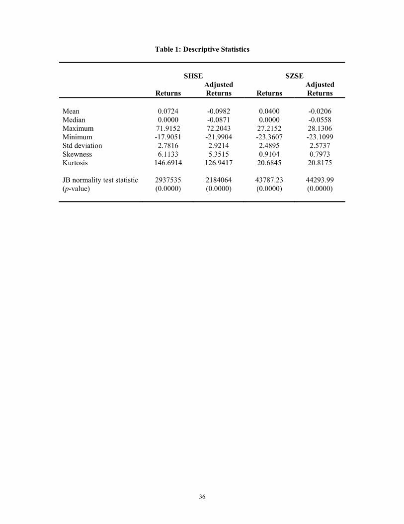
Table 1 provides the descriptive statistics for both the returns and adjusted returns series after

correcting for thin trading. Looking at the mean values, the thin trading adjustment has

resulted in negative average daily returns of -0.10% and -0.02% for both the SHSE and SZSE

respectively, though the magnitudes are not large. In general, the adjustment procedure does

not alter the distribution of both the returns and adjusted returns series. For instance, all

series, both before and after adjustment, exhibit some degree of right-skewness, and are

highly leptokurtic in which the tails of their respective distributions taper down to zero more

gradually than do the tails of a normal distribution. Given the non-zero skewness levels and

excess kurtosis, the Jarque-Bera (JB) test statistic strongly rejects the null of normality for all

series. It is worth highlighting that the analysis in subsequent section is performed only on the

adjusted returns series.

<<Insert Table 1 about here>>

22

5.2 Detecting epochs of linear and nonlinear serial dependencies

This section proceeds to detect brief periods of deviation from a random walk for both stock

exchanges. With a window length of 31 observations, 4 lags are used to compute the

correlations and bicorrelations in each window. As elaborated in earlier section, the research

framework looks for those windows in which the time series exhibit behaviour that departs

significantly from the null hypothesis of pure white noise in terms of linear serial dependence

(significant correlations detected by the C statistic) or nonlinear serial dependence

(significant bicorrelations detected by the H statistic). The results are summarized in Table 2,

highlighting those windows where non-zero correlations or bicorrelations are detected by the

portmanteau test statistics. For the Shanghai data, the null hypothesis is rejected by the C

statistic in 7 windows, which is equivalent to 6.42% of the total windows in our sample. On

the other hand, the presence of strong non-zero bicorrelations has triggered the rejection of

the null hypothesis by the H statistic in 8 windows (7.34%). In the case Shenzhen, the total

numbers of significant C and H windows are 3 (2.80%) and 7 (6.54%) respectively. As a

whole, these findings reveal that the adjusted returns series for both indices follow a random

walk for long periods of time, only to be interspersed with brief periods of strong linear

and/or nonlinear dependency structures. It is worth noting that in all cases, nonlinear

dependence in the adjusted returns series occurs more frequently than the linear correlations,

and hence should not be discarded when examining the weak-form efficiency of a stock

market.

<<Insert Table 2 about here>>

23

Another important implication is that statistical tests employed should be capable of

uncovering epochs of transient temporal dependence. This would facilitate researchers to

identify those events in which their impacts are only grasped over a period of time by

investors, instead of instantaneous responses advocated by the classical EMH (see Brooks et

al., 2000; Rockinger and Urga, 2000; Ammermann and Patterson, 2003; Li, 2003a; Lim et

al., 2006). Nawrocki (1996) hypothesized that economic events are important in generating

temporal dependence in the stock market.9 While his empirical investigation focused on

autocorrelation coefficient, the conjecture applies equally to the formation of nonlinear

dependence. For instance, Hinich and Serletis (2007) postulated that when surprises hit the

market, the adjustment process generally generates a pattern of nonlinear price movements

relative to previous movements, because the traders are unsure of how to react and hence they

respond slowly. Given that informational events are hypothesized to be a source of temporal

dependence, Table 2 provides the time periods during which these linear and nonlinear

dependencies occurred so that future study could identify the major events that contributed to

these gradual market reactions.

Unlike the focus of most conventional efficiency studies, returns predictability in the present

framework accommodates both linear and nonlinear dependencies detected via the C and H

statistics respectively. Hence, plotting both test statistics in a single graph would provide a

better view of the occurrence of serial dependencies over time. For clarity, Figure 2 and 3

plot only those significant C and H windows, while insignificant windows are omitted. The

horizontal axis shows the time window, while the vertical axis is the percentile (i.e. one

9 The sources of index return autocorrelation are still very much been debated in existing literature (see Ahn et al., 2002). One of the explanations given is it reflects delayed price adjustment to the arrival of new information. In fact, several papers have developed formal speed of adjustment estimators to gauge the speed with which new information is reflected in stock prices (see, for example, Amihud and Mendelson, 1989; Damodaran, 1993; Theobald and Yallup, 1998, 2004). These estimators are functions of autocorrelations since both price under- and over-reactions would induce particular autocorrelation patterns into the return series.

24

minus the p-value) for the portmanteau test statistics. Thus, a very significant window is

plotted as a value near 1.0. The dates these series depart from pure white noise either due to

significant C or H statistics or both are provided in the final panel of Table 2. Figure 2 and 3

clearly demonstrate that the adjusted returns for both series follow a pure white noise process

for long periods of time, only to be interspersed with brief periods of strong linear and/or

nonlinear dependency structures. In the case of Shanghai, the series move in a significantly

non-random and dependent pattern in only 12 out of a total 109 time windows, which is

equivalent to 11.01%. Similarly, serial dependencies are detected in only 9.34% of the total

windows for Shenzhen data. This suggests that both stock exchanges in China are efficient

most but not all the time, as strong evidence of episodic serial dependencies indicates delayed

price adjustment to the arrival of new information during those identified sub-periods.

<<Insert Figure 2 about here>>

<<Insert Figure 3 about here>>

25

A careful examination of Figure 2 reveals that serial dependence is detected as early as the

first sub-period of 4/4/1991-5/16/1991 for the adjusted returns series of Shanghai SE

Composite Price Index. However, these dependency structures disappear in subsequent time

windows, only to re-emerge in 1992 (2/3/92-3/16/92 and 9/7/92-10/19/92). This finding is in

contrast to those conducted by Li (2003a) who found a higher degree of predictability at the

early stage of market development up to early 1993. The latter attributed such predictability

partly to market illiquidity. This apparent contradiction is not surprising as our analysis

utilizes returns series that have corrected for the effects of thin trading. Specifically, spurious

autocorrelation brought about by thin trading documented in Li (2003a) has been removed

through the adjustment procedure, and hence the magnitude of serial correlations presence in

the adjusted returns series is substantially reduced. The Shanghai stock market enjoyed two

years of quiescent period following that, with no significant serial dependence been detected

from 10/20/1992-10/26/1994. This relatively long period of market efficiency was again

attained during 10/16/1997-9/9/1999 and 11/17/2000-12/31/2003. Between those years, the

dependency structures appear sporadically with their behaviour being characterized as

episodic.

Figure 3 reveals that serial dependencies in the Shenzhen data exhibit similar episodic

behaviour over the whole sample period. The Shenzhen Stock Exchange also enjoyed three

long periods of market efficiency with each covering more than two years during 2/12/1994-

2/20/1996, 10/21/1997-9/14/1999 and 11/22/2000-12/31/2003. It is worth highlighting that

SHSE also attained efficiency during the last two sub-periods. In fact, after October 1997,

Shenzhen Stock Exchange seems to move hand-in-hand with its Shanghai counterpart. Even

the existence of serial dependencies occurs around the same time period (SHSE: 9/10/1999-

10/22/1999, 12/7/1999-1/18/2000, 10/5/2000-11/16/2000; SZSE: 9/15/1999-10/27/1999,

26

12/10/1999-1/21/2000, 10/10/2000-11/21/2000). This is not surprising given our earlier

observation in Figure 1 that the movements in both indices follow one another closely,

mainly due to the fact that they are driven by the same underlying factors. This is consistent

with the argument of Li (2003a: 356) that the two markets are after all in the same country

and subjected to the influence of the same political, economic, social and institutional

changes. Another interesting observation is that after October 1997, the significant

dependency structures in both markets appear less frequent. This improved market efficiency

can be attributed to a series of regulations and laws promulgated and enforced by the Chinese

authorities during the third development stage (Li, 2003a: 355).

The present findings provide some plausible explanations to the contradicting evidence

documented in earlier studies for both stock exchanges using similar aggregate price indices.

For instance, the unit root test results of Liu et al. (1999) found that both markets are efficient

for the period of 5/21/1992-12/18/1995. However, a closer inspection of Figure 2 and 3

reveals that predictable patterns do exist during this sample period. The failure of the unit

root test is due to two reasons: firstly, the test is not capable of detecting nonlinearity in the

underlying series; secondly, the short burst of linear serial correlations is not strong enough to

cause a rejection in the null hypothesis of the ADF unit root test. Moreover, the unit root test

is not designed to detect predictability (Campbell et al., 1997). In contrast, Mookerjee and Yu

(1999) found that both the SHSE and SZSE are inefficient for the sample period 12/19/1990-

12/17/1993 and 4/3/1991-12/17/1993 respectively. Their inefficiency finding is not surprising

as Table 2 shows that the C statistic detects significant linear dependence during the above

sub-periods. With regard to the conflicting evidence documented in the literature, some

authors (Groenewold et al., 2003; Ma, 2004) argued that examining efficiency over the

largest possible sample sizes might be able to clarify some of the ambiguity. However, this

27

will not be the best solution given the episodic occurrence of serial dependencies, which

would go undetected in full sample analysis.

6. Conclusion

Earlier Chinese efficiency studies assumed that deviation from a random walk is in the form

of linear serial correlations, and market efficiency is a static characteristic that remains

unchanged over the entire estimation period. The inference drawn from autocorrelation-based

tests is on shaky ground due to two major criticisms: (1) evidence of significant

autocorrelation could be the result of thin trading that characterized most emerging stock

markets; (2) the lack of linear correlations does not necessarily imply efficiency as returns

series can be linearly uncorrelated and at the same time nonlinearly dependent. On the other

hand, it is unreasonable to expect the stock market to be efficient all the time. Given the

shortcomings of prior studies, the present paper re-examines the weak-form efficiency of two

Chinese stock markets located in Shanghai and Shenzhen. The methodology proposed by

Miller et al. (1994) is adopted to address the issue of spurious autocorrelation induced by thin

trading, while the test statistics proposed by Hinich and Patterson (1995, 2005) are computed

in non-overlapped moving sub-samples to detect the persistence of linear and nonlinear serial

dependencies over time.

Our main findings can be summarized as follows. Firstly, after correcting for thin trading,

there is still evidence of serial correlations in the adjusted returns series for both markets.

Secondly, nonlinear dependence occurs more frequently than the linear correlations,

justifying the need to test for nonlinearity when examining the weak-form efficiency of a

stock market. Thirdly, the two Chinese markets are found to be efficient most but not all the

28

time. Specifically, their adjusted returns series follow a random walk for long periods of time,

only to be interspersed with brief periods of strong linear and/or nonlinear dependency

structures. This suggests that there are certain time periods when new information is not fully

reflected into stock prices. Though this piece of evidence taken as a whole does not represent

an outright rejection of the weak-form EMH, to view market efficiency as a continuous

variable consistent with the reported empirical results, the adaptive markets hypothesis is a

better framework.

Another interesting finding is that the existence of serial dependencies in both the Shanghai

and Shenzhen Stock Exchanges follows one another closely after October 1997. It suggests

that both markets responded in a similar way to influences from political, economic, social

and institutional changes. In line with our a priori expectation, we do find frequent short

bursts of significant serial dependencies in the earlier stages of market development, but they

appear less frequent when the market matures over time. This can be attributed to a series of

regulations and laws promulgated and enforced by the market regulators during the third

development stage (Li, 2003a: 355). However, the issue of whether the legal environment of

a country matters for stock market efficiency requires further empirical investigations, which

is made possible with data provided by the law and finance literature (see La Porta et al.,

1998). Specifically, this would require extending the present framework to a broad cross-

section of countries, and then explore the determinants for these cross-country differences in

the total number of windows with significant serial dependencies. Besides market

regulations, other potential determinants with accessible country-level data are the degree of

stock market development, market liquidity, returns volatility and the extent of stock market

openness.

29

Acknowledgements

The authors would like to thank Robert D. Brooks for his helpful comments and suggestions

on the earlier version of this paper. The first author thanks Universiti Malaysia Sabah for

offering him a scholarship to pursue his PhD study in Monash University. The usual

disclaimer applies.

References

Abraham, A., F.J. Seyyed and S.A. Alsakran (2002), ‘Testing the Random Walk Behavior and Efficiency of the Gulf Stock Markets’, Financial Review, 37: 469-480.

Ahn, D.H., J. Boudoukh, M. Richardson and R.F. Whitelaw (2002), ‘Partial Adjustment or Stale

Prices? Implications from Stock Index and Futures Return Autocorrelations’, Review of Financial Studies, 15: 655-689.

Al-Khazali, O.M., D.K. Ding and C.S. Pyun (2007), ‘A New Variance Ratio Test of Random

Walk in Emerging Markets: A Revisit’, Financial Review, 42: 303-317. Al-Loughani, N. and D. Chappell (1997), ‘On the Validity of the Weak-form Efficient

Markets Hypothesis Applied to the London Stock Exchange’, Applied Financial Economics, 7: 173-176.

Amihud, Y. and H. Mendelson (1989), ‘Index and Index-futures Returns’, Journal of

Accounting, Auditing and Finance, 4: 415-431. Ammermann, P.A. and D.M. Patterson (2003), ‘The Cross-sectional and Cross-temporal

Universality of Nonlinear Serial Dependencies: Evidence from World Stock Indices and the Taiwan Stock Exchange’, Pacific-Basin Finance Journal, 11: 175-195.

Andrada-Félix, J., F. Fernadez-Rodriguez, M.D. Garcia-Artiles and S. Sosvilla-Rivero

(2003), ‘An Empirical Evaluation of Non-linear Trading Rules’, Studies in Nonlinear Dynamics and Econometrics, 7(3): Article 4.

Antoniou, A., N. Ergul and P. Holmes (1997a), ‘Market Efficiency, Thin Trading and Non-

linear Behaviour: Evidence from an Emerging Market’, European Financial Management, 3: 175-190.

Antoniou, A., N. Ergul, P. Holmes and R. Priestley (1997b), ‘Technical Analysis, Trading

Volume and Market Efficiency: Evidence from an Emerging Market’, Applied Financial Economics, 7: 361-365.

30

Appiah-Kusi, J. and K. Menyah (2003), ‘Return Predictability in African Stock Markets’, Review of Financial Economics, 12: 247-270.

Bailey, W. (1994), ‘Risk and Return on China’s New Stock Markets: Some Preliminary

Evidence’, Pacific-Basin Finance Journal, 2: 243-260. Bailey, W., P. Chung and J.K. Kang (1999), ‘Foreign Ownership Restrictions and Equity

Price Premiums: What Drives the Demand for Cross-border Investments?’, Journal of Financial and Quantitative Analysis, 34: 489-511.

Blasco, N., C.D. Rio and R. Santamaría (1997), ‘The Random Walk Hypothesis in the

Spanish Stock Market: 1980-1992’, Journal of Business Finance and Accounting, 24: 667-683.

Box, G.E.P. and G.M. Jenkins (1970), Times Series Analysis, Forecasting and Control. San

Francisco: Holden-Day. Brooks, C. and M.J. Hinich (1998), ‘Episodic Nonstationarity in Exchange Rates’, Applied

Economics Letters, 5: 719-722. Brooks, C. and M.J. Hinich (1999), ‘Cross-correlations and Cross-bicorrelations in Sterling

Exchange Rates’, Journal of Empirical Finance, 6: 385-404. Brooks, C. and M.J. Hinich (2001), ‘Bicorrelations and Cross-bicorrelations as Non-linearity

Tests and Tools for Exchange Rate Forecasting’, Journal of Forecasting, 20: 181-196. Brooks, C., M.J. Hinich and R. Molyneux (2000), ‘Episodic Nonlinear Event Detection:

Political Epochs in Exchange Rates’, in D. Richards (ed.), Political Complexity: Political Epochs in Exchange Rates, pp. 83-98. Michigan: Michigan University Press.

Campbell, J.Y., A.W. Lo and A.C. MacKinlay (1997), The Econometrics of Financial

Markets. Princeton: Princeton University Press. Chappel, D., J. Padmore and J. Pidgeon (1998), ‘A Note on ERM Membership and the

Efficiency of the London Stock Exchange’, Applied Economics Letters, 5: 19-23. Chen, G., M. Firth and J.B. Kim (2004), ‘IPO Underpricing in China’s New Stock Markets’,

Journal of Multinational Financial Management, 14: 283-302. Clyde, W.C. and C.L. Osler (1997), ‘Charting: Chaos Theory in Disguise?’, Journal of

Futures Markets, 17: 489-514. Damodaran, A. (1993), ‘A Simple Measure of Price Adjustment Coefficients’, Journal of Finance,

48: 387-400. Darrat, A.F. and M. Zhong (2000), ‘On Testing the Random-walk Hypothesis: A Model

Comparison Approach’, Financial Review, 35: 105-124.

31

De Long, J.B., A. Shleifer, L.H. Summers and R.J. Waldmann (1990), ‘Positive Feedback Investment Strategies and Destabilizing Rational Speculation’, Journal of Finance, 45: 379-395.

Emerson, R., S.G. Hall and A. Zalewska-Mitura (1997), ‘Evolving Market Efficiency with an

Application to Some Bulgarian Shares’, Economics of Planning, 30: 75-90. Fernández-Rodríguez, F., C. González-Martel and S. Sosvilla-Rivero (2000), ‘On the

Profitability of Technical Trading Rules based on Artificial Neural Networks: Evidence from the Madrid Stock Market’, Economics Letters, 69: 89-94.

Freund, W.C., M. Larrain and M.S. Pagano (1997), ‘Market Efficiency Before and After the

Introduction of Electronic Trading at the Toronto Stock Exchange’, Review of Financial Economics, 6: 29-56.

Freund, W.C. and M.S. Pagano (2000), ‘Market Efficiency in Specialist Markets Before and

After Automation’, Financial Review, 35: 79-104. Gençay, R. (1998), ‘The Predictability of Security Returns with Simple Technical Trading

Rules’, Journal of Empirical Finance, 5: 347-359. Girardin, E. and Z. Liu (2003), ‘The Chinese Stock Market: A Casino with ‘Buffer Zones’?’,

Journal of Chinese Economic and Business Studies, 1: 57-70. Gordon, R.H. and W. Li (2003), ‘Government as a Discriminating Monopolist in the

Financial Market: The Case of China’, Journal of Public Economics, 87: 283-312. Granger, C.W.J. (1983), ‘Forecasting White Noise’, in A. Zellner (ed.), Applied Time Series

Analysis of Economic Data, Proceedings of the Conference on Applied Time Series Analysis of Economic Data, pp.308-314. Washington, DC: U.S. Government Printing Office.

Granger, C.W.J. and A.P. Andersen (1978), An Introduction to Bilinear Time Series Models.

Gottingen: Vandenhoeck and Ruprect. Groenewold, N., S.H.K. Tang and Y. Wu (2003), ‘The Efficiency of the Chinese Stock

Market and the Role of the Banks’, Journal of Asian Economies, 14: 593-609. Groenewold, N., Y. Wu, S.H.K. Tang and X.M. Fan (2004), The Chinese Stock Market:

Efficiency, Predictability and Profitability. Cheltenham: Edward Elgar. Hamill, P.A., K.K. Opong and D. Sprevak (2000), ‘The Behaviour of Irish ISEQ Index: Some

New Empirical Tests’, Applied Financial Economics, 10: 693-700. Hassan, K.M., W.S. Al-Sultan and J.A. Al-Saleem (2003), ‘Stock Market Efficiency in the

Gulf Cooperation Council Countries (GCC): The Case of Kuwait Stock Exchange’, Scientific Journal of Administrative Development, 1: 1-21.

32

He, Y., C. Wu and Y.M. Chen (2003), ‘An Explanation of the Volatility Disparity between the Domestic and Foreign Shares in the Chinese Stock Markets’, International Review of Economics and Finance, 12: 171-186.

Hinich, M.J. (1996), ‘Testing for Dependence in the Input to a Linear Time Series Model’,

Journal of Nonparametric Statistics, 6: 205-221. Hinich, M.J. and A. Serletis (2007), ‘Episodic Nonlinear Event Detection in the Canadian

Exchange Rate’, Journal of the American Statistical Association, 102: 68-74. Hinich, M.J. and D.M. Patterson (1985), ‘Evidence of Nonlinearity in Daily Stock Returns’,

Journal of Business and Economic Statistics, 3: 69-77. Hinich, M.J. and D.M. Patterson (1995), ‘Detecting Epochs of Transient Dependence in

White Noise’, Mimeo, University of Texas at Austin. Hinich, M.J. and D.M. Patterson (2005), ‘Detecting Epochs of Transient Dependence in

White Noise’, in M.T. Belongia and J.M. Binner (eds.), Money, Measurement and Computation, pp.61-75. London: Palgrave Macmillan.

Jefferis, K. and G. Smith (2004), ‘Capitalisation and Weak-form Efficiency in the JSE

Securities Exchange’, South African Journal of Economics, 72: 684-707. Jefferis, K. and G. Smith (2005), ‘The Changing Efficiency of African Stock Markets’, South

African Journal of Economics, 73: 54-67. Jenkins, G.M. and D. Watts (1968), Spectral Analysis and Its Applications. San Francisco:

Holden-Day. Kang, J., M.H. Liu and S.X. Ni (2002), ‘Contrarian and Momentum Strategies in the China

Stock Market: 1993-2000’, Pacific-Basin Finance Journal, 10: 243-265. Kohers, T., V. Pandey and G. Kohers (1997), ‘Using Nonlinear Dynamics to Test for Market

Efficiency among the Major U.S. Stock Exchanges’, Quarterly Review of Economics and Finance, 37: 523-545.

La Porta, R., F. Lopez-de-Silanes, A. Shleifer and R. Vishny (1998), ‘Law and Finance’,

Journal of Political Economy, 106: 1113-1155. Laurence, M., F. Cai and S. Qian (1997), ‘Weak-form Efficiency and Causality Tests in

Chinese Stock Markets’, Multinational Finance Journal, 1: 291-307. Lee, C.F., G.M. Chen and O.M. Rui (2001), ‘Stock Returns and Volatility on China’s Stock

Markets’, Journal of Financial Research, 24: 523-543. Li, X.M. (2003a), ‘China: Further Evidence on the Evolution of Stock Markets in Transition

Economies’, Scottish Journal of Political Economy, 50: 341-358. Li, X.M. (2003b), ‘Time-varying Informational Efficiency in China’s A-share and B-share

Markets’, Journal of Chinese Economic and Business Studies, 1: 33-56.

33

Lim, K.P., M.J. Hinich and R.D. Brooks (2006), ‘Events that Shook the Market: An Insight from Nonlinear Serial Dependencies in Intraday Returns’, SSRN Working Paper, available at http://ssrn.com/abstract=912603.

Lima, E.J.A. and B.M. Tabak (2004), ‘Tests of the Random Walk Hypothesis for Equity

Markets: Evidence from China, Hong Kong and Singapore’, Applied Economics Letters, 11: 255-258.

Liu, X., H. Song and P. Romilly (1997), ‘Are Chinese Stock Markets Efficient? A

Cointegration and Causality Analysis’, Applied Economics Letters, 4: 511-515. Lo, A.W. (2004), ‘The Adaptive Markets Hypothesis: Market Efficiency from an

Evolutionary Perspective’, Journal of Portfolio Management, 30: 15-29. Lo, A.W. (2005), ‘Reconciling Efficient Markets with Behavioral Finance: The Adaptive

Markets Hypothesis’, Journal of Investment Consulting, 7(2): 21-44. Lo, A.W. and A.C. MacKinlay (1988), ‘Stock Market Prices do not Follow Random Walk:

Evidence from a Simple Specification Test’, Review of Financial Studies, 1: 41-66. Lo, A.W. and A.C. Mackinlay (1989), ‘The Size and Power of the Variance Ratio in Finite

Samples’, Journal of Econometrics, 40: 203-238. Lo, A.W. and A.C. MacKinlay (1990), ‘An Econometric Analysis of Nonsynchronous

Trading’, Journal of Econometrics, 45: 181-212. Long, D.M., J.D. Payne and C. Feng (1999), ‘Information Transmission in the Shanghai

Equity Market’, Journal of Financial Research, 22: 29-45. Ma, S. (2004), The Efficiency of China’s Stock Market. Aldershot: Ashgate. Ma, X. (1996), ‘Capital Controls, Market Segmentation and Stock Prices: Evidence from the

Chinese Stock Market’, Pacific-Basin Finance Journal, 4: 219-239. Maghyereh, A. (2005), ‘Electronic Trading and Market Efficiency in an Emerging Market:

The Case of the Jordanian Capital Market’, Emerging Markets Finance and Trade, 41(4): 5-19.

Miller, M.H., J. Muthuswamy and R.E. Whaley (1994), ‘Mean Reversion of Standard and

Poor’s 500 Index Basis Changes: Arbitrage-induced or Statistical Illusion? Journal of Finance, 49: 479-513.

Mok, H.M.K. and Y.V. Hui (1998), ‘Underpricing and Aftermarket Performance of IPOs in

Shanghai, China’, Pacific-Basin Finance Journal, 6: 453-474. Mookerjee, R. and Q. Yu (1999), ‘An Empirical Analysis of the Equity Markets in China’,

Review of Financial Economics, 8: 41-60.

34

Nam, S.K., K.S. Park and Y.K. Kim (1999), ‘Agenda for Capital Market Reforms in the PRC’, in ADB, A Study of Financial Markets, Vol.4: People’s Republic of China, pp.68-98. Manila: ADB.

Narayan, P.K. (2005), ‘Are the Australian and New Zealand Stock Prices Nonlinear with a

Unit Root?’ Applied Economics, 37: 2161-2166. Nawrocki, D.N. (1996), ‘Market Dependence and Economic Events’, Financial Review, 31:

287-312. Neftci, S.N. (1991), ‘Naive Trading Rules in Financial Markets and Wiener-Kolmogorov

Prediction Theory: A Study of “Technical Analysis”’, Journal of Business, 64: 549-571.

Opong, K.K., G. Mulholland, A.F. Fox and K. Farahmand (1999), ‘The Behavior of Some

UK Equity Indices: An Application of Hurst and BDS Tests’, Journal of Empirical Finance, 6: 267-282.

Panagiotidis, T. (2005), ‘Market Capitalization and Efficiency: Does it Matter? Evidence

from the Athens Stock Exchange’, Applied Financial Economics, 15: 707-713. Poshakwale, S. (2002), ‘The Random Walk Hypothesis in the Emerging Indian Stock

Market’, Journal of Business Finance and Accounting, 29: 1275-1299. Qi, D., W. Wu and H. Zhang (2000), ‘Shareholding Structure and Corporate Performance of

Partially Privatized Firms: Evidence from Listed Chinese Companies’, Pacific-Basin Finance Journal, 8: 587-610.

Rahman, A.H. and S. Saadi (2007), ‘Is South Korea’s Stock Market Efficient? A Note’,

Applied Economics Letters, 14: 71-74. Rahman, A.H. and S. Saadi (2008), ‘Random Walk and Breaking Trend in Financial Series:

An Econometric Critique of Unit Root Tests’, Review of Financial Economics, 17: 204-212.

Rayhorn, C., M.K. Hassan, J.S. Yu and K.R. Janson (2007), ‘Emerging Market Efficiencies:

New Zealand's Maturation Experience in the Presence of Non-linearity, Thin Trading and Asymmetric Information’, International Review of Finance, 7: 21-34.

Rockinger, M. and G. Urga (2000), ‘The Evolution of Stock Markets in Transition

Economies’, Journal of Comparative Economics, 28: 456-472. Rockinger, M. and G. Urga (2001), ‘A Time Varying Parameter Model to Test for

Predictability and Integration in Stock Markets of Transition Economies’, Journal of Business and Economic Statistics, 19: 73-84.

Saadi, S., D. Gandhi and S. Dutta (2006a), ‘Testing for Nonlinearity and Modeling Volatility

in Emerging Capital Markets: The Case of Tunisia’, International Journal of Theoretical and Applied Finance, 9: 1021-1050.

35

Saadi, S., D. Gandhi and K. Elmawazini (2006b), ‘On the Validity of Conventional Statistical Tests Given Evidence of Non-synchronous Trading and Non-linear Dynamics in Returns Generating Process’, Applied Economics Letters, 13: 301-305.

Sarantis, N. (2001), ‘Nonlinearities, Cyclical Behaviour and Predictability in Stock Markets:

International Evidence’, International Journal of Forecasting, 17: 459-482. Seddighi, H.R. and W. Nian (2004), ‘The Chinese Stock Exchange Market: Operations and

Efficiency’, Applied Financial Economics, 14: 785-797. Self, J.K. and I. Mathur (2006), ‘Asymmetric Stationarity in National Stock Market Indices:

An MTAR Analysis’, Journal of Business, 79: 3153-3174. Su, D. and B.M. Fleisher (1999a), ‘An Empirical Investigation of Underpricing in Chinese

IPOs’, Pacific-Basin Finance Journal, 7: 173-202. Su, D. and B.M. Fleisher (1999b), ‘Why does Return Volatility Differ in Chinese Stock

Markets?’, Pacific-Basin Finance Journal, 7: 557-586. Sun, Q. and W.H.S. Tong (2000), ‘The Effect of Market Segmentation on Stock Prices: The

China Syndrome’, Journal of Banking and Finance, 24: 1875-1902. Theobald, M. and P. Yallup (1998), ‘Measuring Cash-futures Temporal Effects in the UK

Using Partial Adjustment Factors’, Journal of Banking and Finance, 22: 221-243. Theobald, M. and P. Yallup (2004), ‘Determining Security Speed of Adjustment

Coefficients’, Journal of Financial Markets, 7: 75-96. Tian, G.G., G.H. Wan and M. Guo (2002), ‘Market Efficiency and the Returns to Simple

Technical Trading Rules: New Evidence from U.S. Equity Market and Chinese Equity Markets’, Asia-Pacific Financial Markets, 9: 241-258.

Wei, Z. and O. Varela (2003), ‘State Equity Ownership and Firm Market Performance:

Evidence from China’s Newly Privatized Firms’, Global Finance Journal, 14: 65-82. Zalewska-Mitura, A. and S.G. Hall (1999), ‘Examining the First Stages of Market

Performance: A Test for Evolving Market Efficiency’, Economics Letters, 64: 1-12. Zalewska-Mitura, A. and S.G. Hall (2000), ‘Do Market Participants Learn? The Case of the

Budapest Stock Exchange’, Economics of Planning, 33: 3-18.

36

Table 1: Descriptive Statistics

SHSE

SZSE

Returns

Adjusted Returns

Returns

Adjusted Returns

Mean

0.0724

-0.0982

0.0400

-0.0206

Median 0.0000 -0.0871 0.0000 -0.0558 Maximum 71.9152 72.2043 27.2152 28.1306 Minimum -17.9051 -21.9904 -23.3607 -23.1099 Std deviation 2.7816 2.9214 2.4895 2.5737 Skewness 6.1133 5.3515 0.9104 0.7973 Kurtosis 146.6914 126.9417 20.6845 20.8175 JB normality test statistic (p-value)

2937535 (0.0000)

2184064 (0.0000)

43787.23 (0.0000)

44293.99 (0.0000)

37

Table 2: Correlation and Bicorrelation Tests in Moving Time Windows

SHSE_ADR

SZSE_ADR

Total number of windows

109

107

Total number of significant C windows

7

3

Dates of significant C windows

4/4/91-5/16/91 (0.0086) 2/3/92-3/16/92 (0.0197)

10/10/95-11/21/95 (0.0241) 12/17/96-1/28/97 (0.0075) 1/29/97-3/12/97 (0.0075) 9/10/99-10/22/99 (0.0175) 10/5/00-11/16/00 (0.0202)

3/3/93-4/14/93 (0.0191) 9/25/96-11/6/96 (0.0227)

10/10/00-11/21/00 (0.0167)

Total number of significant H windows

8

7

Dates of significant H windows

4/4/91-5/16/91 (0.0000) 9/7/92-10/19/92 (0.0002)

10/27/94-12/8/94 (0.0022) 4/1/96-5/13/96 (0.0025) 1/29/97-3/12/97 (0.0077) 9/3/97-10/15/97 (0.0064) 9/10/99-10/22/99 (0.0000) 12/7/99-1/18/00 (0.0005)

9/30/91-11/11/91 (0.0109) 12/31/93-2/11/94 (0.0007) 2/21/96-4/3/96 (0.0010) 4/4/96-5/16/96 (0.0000) 9/8/97-10/20/97 (0.0102) 9/15/99-10/27/99 (0.0006) 12/10/99-1/21/00 (0.0021)

Total number of significant C and H windows

12

10

Dates of significant C and H windows

4/4/91-5/16/91 2/3/92-3/16/92 9/7/92-10/19/92 10/27/94-12/8/94 10/10/95-11/21/95

4/1/96-5/13/96 12/17/96-1/28/97 1/29/97-3/12/97 9/3/97-10/15/97 9/10/99-10/22/99 12/7/99-1/18/00 10/5/00-11/16/00

9/30/91-11/11/91 3/3/93-4/14/93

12/31/93-2/11/94 2/21/96-4/3/96 4/4/96-5/16/96 9/25/96-11/6/96 9/8/97-10/20/97 9/15/99-10/27/99 12/10/99-1/21/00 10/10/00-11/21/00

Notes: SHSE_ADR- Adjusted returns series for Shanghai SE Composite Price Index SZSE_ADR- Adjusted returns series for Shenzhen SE Composite Price Index

Values in parentheses indicate the p-values of the test statistics

38

Figure 1: Time Series Plots for Chinese Stock Market Indices

Shanghai SE Composite Price Index

0

200

400

600

800

1000

1200

1400

1600

1800

2000

2200

24001/

2/91

7/2/

91

1/2/

92

7/2/

92

1/2/

93

7/2/

93

1/2/

94

7/2/

94

1/2/

95

7/2/

95

1/2/

96

7/2/

96

1/2/

97

7/2/

97

1/2/

98

7/2/

98

1/2/

99

7/2/

99

1/2/

00

7/2/

00

1/2/

01

7/2/

01

1/2/

02

7/2/

02

1/2/

03

7/2/

03

Shenzhen SE Composite Price Index

0

100

200

300

400

500

600

700

4/3/

91

10/3

/91

4/3/

92

10/3

/92

4/3/

93

10/3

/93

4/3/

94

10/3

/94

4/3/

95

10/3

/95

4/3/

96

10/3

/96

4/3/

97

10/3

/97

4/3/

98

10/3

/98

4/3/

99

10/3

/99

4/3/

00

10/3

/00

4/3/

01

10/3

/01

4/3/

02

10/3

/02

4/3/

03

10/3

/03

Figure 2: Significant C and H Windows for Adjusted Returns Series of SHSE

0.00

0.10

0.20

0.30

0.40

0.50

0.60

0.70

0.80

0.90

1.00

1/8/

91

8/13

/91

3/17

/92

10/2

0/92

5/25

/93

12/2

8/93

8/2/

94

3/7/

95

10/1

0/95

5/14

/96

12/1

7/96

7/22

/97

2/24

/98

9/29

/98

5/4/

99

12/7

/99

7/11

/00

2/13

/01

9/18

/01

4/23

/02

11/2

6/02

7/1/

03

C H

40

Figure 3: Significant C and H Windows for Adjusted Returns Series of SZSE

0.00

0.10

0.20

0.30

0.40

0.50

0.60

0.70

0.80

0.90

1.00

4/9/

91

11/1

2/91

6/16

/92

1/19

/93

8/24

/93

3/29

/94

11/1

/94

6/6/

95

1/9/

96

8/13

/96

3/18

/97

10/2

1/97

5/26

/98

12/2

9/98

8/3/

99

3/7/

00

10/1

0/00

5/15

/01

12/1

8/01

7/23

/02

2/25

/03

9/30

/03

C H