efficiency and risk in european banking by franco
TRANSCRIPT

© European Central Bank, 2010
AddressKaiserstrasse 2960311 Frankfurt am Main, Germany
Postal addressPostfach 16 03 1960066 Frankfurt am Main, Germany
Telephone+49 69 1344 0
Internethttp://www.ecb.europa.eu
Fax+49 69 1344 6000
All rights reserved.
Any reproduction, publication and reprint in the form of a different publication, whether printed or produced electronically, in whole or in part, is permitted only with the explicit written authorisation of the ECB or the authors.
Information on all of the papers published in the ECB Working Paper Series can be found on the ECB’s website, http://www.ecb.europa.eu/pub/scientific/wps/date/html/index.en.html
ISSN 1725-2806 (online)
Macroprudential Research Network
This paper presents research conducted within the Macroprudential Research Network (MaRs). The network is composed of econo-mists from the European System of Central Banks (ESCB), i.e. the 27 national central banks of the European Union (EU) and the Euro-pean Central Bank. The objective of MaRs is to develop core conceptual frameworks, models and/or tools supporting macro-prudential supervision in the EU.
The research is carried out in three work streams:1. Macro-fi nancial models linking fi nancial stability and the performance of the economy;2. Early warning systems and systemic risk indicators;3. Assessing contagion risks.
MaRs is chaired by Philipp Hartmann (ECB). Paolo Angelini (Banca d’Italia), Laurent Clerc (Banque de France), Carsten Detken (ECB) and Katerina Šmídková (Czech National Bank) are workstream coordinators. Xavier Freixas (Universitat Pompeu Fabra) acts as external consultant and Angela Maddaloni (ECB) as Secretary.
The refereeing process of this paper has been coordinated by a team composed of Cornelia Holthausen, Kalin Nikolov and Bernd Schwaab (all ECB).
The paper is released in order to make the research of MaRs generally available, in preliminary form, to encourage comments and sug-gestions prior to fi nal publication. The views expressed in the paper are the ones of the author(s) and do not necessarily refl ect those of the ECB or of the ESCB.
3ECB
Working Paper Series No 1211June 2010
Abstract 4
Non-technical summary 5
1 Introduction 6
2 Related literature 8
3 Research hypothesis 11
4 Methodology 13
5 Variables and data 16
6 Results 19
7 Robustness tests 21
8 Conclusions 23
References TablesAppendix
CONTENTS
25
29
35

4ECBWorking Paper Series No 1211June 2010
Abstract We analyze the impact of efficiency on bank risk. We also consider whether bank capital has
an effect on this relationship. We model the inter-temporal relationships among efficiency,
capital and risk for a large sample of commercial banks operating in the European Union. We
find that reductions in cost and revenue efficiencies increase banks’ future risks thus
supporting the bad management and efficiency version of the moral hazard hypotheses. In
contrast, bank efficiency improvements contribute to shore up bank capital levels. Our
findings suggest that banks lagging behind in their efficiency levels might expect higher risk
and subdued capital positions in the near future.
Keywords: banking risk; capital; efficiency
JEL classification: G21; D24; C23; E44

5ECB
Working Paper Series No 1211June 2010
Non-technical summary
Following a process of de-regulation and innovation in credit markets over the two decades prior to the credit crisis that started in late 2007 European banking markets became increasingly integrated and more competitive. As a result of this process, there have been stronger pressures on banks’ capital and a stronger emphasis on the importance of improved efficiency in the banking sector. That is, it forced banks to operate closer to the “best practice” or efficient production function.
Our aim is, first, to assess the impact of efficiency on bank risk. In this respect low levels of efficiency could lead banks to try to boost their performance via laxer credit standards and/or less intensive monitoring of credit. In turn, we will also have to consider if changes in bank risk have an influence on their efficiency levels. For instance, increases in bank risk may temporally precede a decline in cost efficiency related to lower credit screening.
Second, we aim to assess the impact of bank capital on the risk and efficiency trade-offs. Namely the relationship between efficiency and risk might be affected by the level of capital particularly in light of the decline of overall bank capital (as a proportion of total loans) at the macroeconomic level. For instance, moral hazard problems might increase incentives of thinly capitalized banks to augment their level of risk thereby incurring higher non-performing loans in the future.
To tackle these questions, we build on previous literature and asses the inter-temporal relationships between bank risk, efficiency and capital levels.2 We use a large data set of European Union commercial banks from 26 European Union countries (EU-26) ranging from 1995 to 2007.
We use Granger-causality methods (Berger and De Young 1997, Williams 2004) in a panel data framework. Our model delves in the relationship between these factors by including several definitions of bank efficiency (i.e. cost, revenue and profit efficiency scores), risk (i.e. non-performing loans and probability of default) and capital (i.e. core equity and total capital).
In general, our results show that subdued bank efficiency (cost or revenue) Granger causes higher risk supporting the “bad management” hypothesis. We also show that increases in bank capital precede cost efficiency improvements suggesting that moral hazard incentives appear to fall as bank capital increases. Cost (and profit) efficiencies are also found to positively Granger-cause bank capital. In other words more efficient banks seem to eventually become more capitalized and higher capital also tend to have a positive effect on efficiency levels.
Overall we believe our results to be particularly interesting from a prudential supervisory perspective. The findings showing that low efficiency scores can harbinger future banking problems and that efficiency improvements tend to shore up banks’ capital positions could be useful from a policy perspective. They emphasize the importance of attaining long-term efficiency gains also to support financial stability objectives.
2 We focus on bank risk-taking, efficiency and capital level since these factors are free of measurement errors. Regarding the
bank competition, there are various measures available (Goddard and Wilson, 2009), but it is still debated which one is the
most accurate (Carbo et al., 2009).

6ECBWorking Paper Series No 1211June 2010
1. Introduction Over the last two decades prior to the credit crisis that started in late 2007, European banking
markets became increasingly integrated. The twin forces of deregulation and technological
change contributed to the progressive process of financial integration and increased
competition in the financial services industry (ECB, 2010).3 As a result of this process, there
has been a tremendous emphasis on the importance of improved efficiency in the banking
sector. That is, it has forced banks to operate closer to the “best practice” or efficient
production function. At the same time, this increase in competition could – at least in the
short term – lead to greater (and possibly excessive) risk-taking. This is because increased
competition reduces the market power of banks thereby decreasing their charter value. The
decline in banks´ charter values coupled with the banks’ limited liability and the existence of
‘quasi’ flat rate deposit insurance could encourage banks to take on more risk (Matutes and
Vives, 2000 and Salas and Saurina, 2003).4 Regulators have tried to counterbalance these
possible incentives by giving capital adequacy a more prominent role in the prudential
regulatory process.5
In this environment a number of studies have focused on the impact of capital
(Repullo, 2004; Allen et al., 2009; Gropp and Heider, 2010), operating efficiency (Casu and
Girardone, 2009a) and business models (Demirgüc-Kunt and Huizinga, 2010) on bank risk.6
3 See Goddard et al (2007).
4 This issue is not undisputed; Boyd and Nicolo (2005) argue that the theoretical foundations linking more competition with
increased incentives towards bank risk-taking are fragile. See Carletti and Hartmann (2002) for a useful survey of the
literature linking competition and stability.
5 For instance, in the aftermath of the introduction of the euro, Vives (2000, pg. 15) already argued that ‘the general trend is
to introduce competition in banking and to check risk- taking with capital requirements and appropriate supervision’.
6 A parallel literature has analysed the impact of bank competition on banks’ risk and efficiency (e.g. Boyd and De Nicolo,
2003; De Nicolo et al., 2008, Cihak, Schaeck and Wolfe, 2009, Casu and Girardone, 2009).

7ECB
Working Paper Series No 1211June 2010
Surprisingly, there are only a limited number of studies that assess inter-temporal relationships
between bank risk, capital and efficiency. The recent credit crisis has highlighted the need for
further understanding of the determinants of bank risk in an environment of enhanced bank
efficiency and lower bank capital (Haldane and Alessandri, 2009).
Our aim is, first, to assess the impact of efficiency on bank risk. In this respect low
levels of efficiency could lead banks to try to boost their performance via laxer standards
and/or less intensive monitoring of credit.7 In turn, we will also have to consider if changes in
bank risk have an influence on efficiency levels. For instance, increases in bank risk may
temporally precede a decline in cost efficiency related to lower credit screening.
Second, we aim to assess the impact of bank capital on risk and efficiency trade-offs.
Namely, the relationship between efficiency and risk might be affected by the level of capital
particularly in light of a decline in overall bank capital (as a proportion of total loans) at the
macroeconomic level. For instance, moral hazard problems might increase incentives of
thinly capitalized banks to augment their level of risk thereby incurring higher non-
performing loans in the future. Similarly, highly capitalized banks may be subject to lower
moral hazard problems and may be both more efficient and prudent than thinly capitalized
institutions. Conversely, as capital is costly highly capitalized banks may, on average,
increase their level of risk to maximize revenues.
To tackle these questions, we build on previous literature and assess the inter-
temporal relationships between bank risk, efficiency and capital levels. We use a large data
set of banks from 26 European Union countries (EU-26) ranging from 1995 to 2007. Our main
variables of interest include both forward and backward-looking measures of bank risk, several
measures of bank capital and three bank efficiency measures (revenue, cost and profit
efficiencies).
7 See section 3 for a detailed description of the main hypotheses.

8ECBWorking Paper Series No 1211June 2010
The rest of this paper is organized as follows: section 2 includes a literature review
while section 3 presents the main hypotheses of interest. The model specification, variables
and data are explained in sections 4 and 5. Section 6 discusses the empirical results, section 7
presents the robustness checks and section 8 concludes.
2. Related literature Bankruptcies in the financial sector are costly, not only for banks’ equity and debt holders but
often also for taxpayers. As a result the study of the determinants of banks’ risk and, in
particular, of the effectiveness of forcing banks to hold a certain amount of capital (to
buttress bank stability) has a long history. An early line of US research on risk-taking
incentives examined the effects of capital regulations (e.g. Peltzman, 1970 or Mayne, 1972).8
The main concern of these early studies was to analyse the effectiveness of financial
regulation and, especially, to consider whether the existence of a flat-rate deposit insurance
scheme (i.e. not linked to banks’ risk) created incentives for excessive risk. Overall, results
from these earlier studies were sceptical about the effectiveness of banking capital regulation
influencing banks’ soundness (see Marcus, 1983).
The introduction of the 1988 Basel Accord on international bank capital standards
(Basel I) reignited interest on the effectiveness of bank capital regulations. A new wave of
studies (mostly for the US banking sector)9 tended to find that regulatory capital constraints
were buttressing banks’ capital (e.g. Wall and Peterson, 1987 and Dahl and Shrieves, 1990).
In the aftermath of the Basel I application and subsequent amendments, the interest on the
effects of capital adequacy regulations on banks´ risk persisted. For instance, Ediz et al.,
(1997) found that bank capital regulation had been effective in increasing capital ratios
8 Most of these earlier approaches build on Friedman’s (1962) capital adjustment model.
9 One exception is Barrios and Blanco (2003).
9ECB
Working Paper Series No 1211June 2010
without substantially shifting bank portfolios and off-balance-sheet (OBS) exposures towards
riskier assets in the US and UK. In this direction also, Demsetz et al., (1996) and Salas and
Saurina (2003) found that banks with lower capital tended to operate with higher levels of
credit risk in line with the moral hazard hypothesis.
In parallel, and depending on the focus and modelling strategy, the theoretical
literature offers contradictory results as to the effects of capital requirements on bank risk-
taking incentives (see Berger et al., 1995; Freixas and Rochet, 2008; Santos, 1999; Boot et
al., 1998). Overall then, the issue of whether higher capital ratios reduce overall banking risk
has remained largely unresolved.
A major contribution to the debate came from Hughes and Mester (1998, 2009) who
argued for the need to consider bank efficiency when analysing the relationship between
capital and risk. According to Hughes and Mester (1998, 2009) both capital and risk are
likely to be determined by the level of bank efficiency. For instance, supervisory authorities
may allow efficient banks (with high quality management) a greater flexibility in terms of
their capital leverage or overall risk profile, ceteris paribus. On the other hand, a less
efficient bank with low capital may be tempted to take on higher risk to compensate for lost
returns due to moral hazard considerations.
In this line Berger and De Young (1997) and Kwan and Eisenbeis (1997) posit that it
is crucial to recognise explicitly the concept of bank efficiency in empirical models analysing
the determinants of banks´ risk.10 Berger and De Young (1997) employ Granger-causality
methods to assess the inter-temporal relationships among problem loans, cost efficiency, and
capital for a sample of US banks from 1985 to 1994. Kwan and Eisenbeis (1997) use a
simultaneous equation framework to test hypotheses about the interrelationships between
10 Pastor and Serrano (2005) also examine the link between efficiency and risk-taking.
10ECBWorking Paper Series No 1211June 2010
bank risk, capitalization, and operating efficiency. Both papers provide evidence that both
efficiency and capital are relevant determinants of bank risk.
Berger and De Young (1997) show that declines in cost efficiency precede increases
in problem loans (particularly at thinly capitalised banks). They also show that problem loans
result in reductions in cost efficiency. Kwan and Eisenbeis (1997) also found that poorly
performing banks are more vulnerable to risk-taking. They also find that that highly
capitalised banks are more efficient than less capitalised institutions.
Williams (2004) and Altunbas et al., (2007) have replicated both papers in a European
banking setting. Similar to Berger and De Young (1997), Williams (2004) uses Granger-
causality techniques to assess the inter-temporal relationships among problem loans, cost
efficiency, and financial capital. His sample includes European savings banks over the period
1990-1998 and finds that poorly managed banks tend to make more poor quality loans.
Altunbas et al., (2007) follow an approach similar to Kwan and Eisenbeis (1997) and use a
static simultaneous equation framework to investigate the relationship between capital, loan
provisions and cost efficiency for a sample of European banks over the period 1992-2000. In
stark contrast to Williams (2004), Altunbas et al., (2007) do not find a positive relationship
between inefficiency and bank risk-taking. Inefficient European banks appear to hold more
capital and take on less risk. Overall, the European studies yield contradictory findings as to
the relationships between operating efficiency, capital and bank risk.
This paper sheds light on the relationship between bank efficiency, capital and risk in
the European Union extending the established literature in three dimensions. First unlike
previous studies our sample includes contemporaneous banking data from the 2000s. That is,
for the first time the data also covers the period of monetary union that has led to radical
changes in the European financial system increasing banks’ pressures towards operate more
efficiently (Goddard et al., 2007, Bos and Schmiedel, 2007). Second, compared with earlier
11ECB
Working Paper Series No 1211June 2010
studies we investigate the risk-efficiency-capital relationships by constructing a broader set of
variables accounting for each of these concepts. While previous studies mostly focus either on
cost efficiency (e.g. Kwan and Eisenbeis 1997, Berger and DeYoung 1997, Williams 2004,
Altunbas et al., 2007) or profit efficiency (Berger and Bonaccorsi 2006), we estimate both cost
and revenue efficiency estimators (and do robustness checks with a profit efficiency measure). We
focus on cost and revenue efficiencies as they reflect two different managerial abilities (i.e.
the abilities to maximize revenues and minimize costs respectively). We posit that each of
these measures can have a different link with bank risk and capital levels (see section 3). In
line with previous studies we include a measure of bank risk derived from banks’ financial
statements (i.e. non-performing loans and total loans). We complement this measure with a
forward-looking indicator of bank risk capturing the financial markets’ view of banks’
likelihood of default obtained from Moodys-KMV. Compared to previous studies we also resort
to a wider measure of bank capital (i.e. total capital instead of equity capital). Finally, we also
extend the earlier literature by using an econometric modelling framework that embeds Granger
causality estimations in a GMM framework.11 Previous studies mostly rely on OLS
estimation but this may be problematic since the introduction of a lagged dependent variable
among the predictors creates complications as the lagged dependent variable is often strongly
correlated with the disturbance term.
3. Research hypotheses Before introducing the empirical model and building on previous studies, we posit the major
research hypotheses about the inter-temporal relationship between bank risk, capital and
efficiency building on Berger and DeYoung (1997) and Kwan and Eisenbeis 1997.
11 See Casu and Girardone (2009) for an application of this estimation procedure to banking.
12ECBWorking Paper Series No 1211June 2010
Banks’ efficiency levels may impact on future bank risk. In what Berger and
DeYoung (1997), and Williams (2004) labeled as the “bad management” hypothesis, banks
operating with low levels of efficiency have higher costs largely due to inadequate credit
monitoring and inefficient control of operating expenses (which is reflected in lower cost
efficiency almost immediately). Declines in cost (and revenue) efficiency will temporally
precede increases in banks’ risk due to credit, operational, market and reputational problems.
The “cost skimping” hypothesis assumes that there is a trade-off between short-term
cost efficiency and future risk-taking due to moral hazard considerations. In such cases,
banks appear to be more cost efficient as they devote fewer resources to credit screening and
monitoring. As a result the stock of non-performing loans remains unaffected in the short run.
In the medium term however, banks reach higher risk levels as they have to purchase the
additional inputs necessary to administer future higher risks. In the case of revenue
efficiency, higher levels of short-term profits are normally obtained at the cost of laxer credit
screening. This will also normally result in higher future risks. In other words, a bank may be
tempted to increase revenues simply by taking on higher risks to compensate for lost returns.
The “bad luck” hypothesis is related to the consequences of increases in bank risk on
efficiency levels. It argues that external exogenous events (e.g., unexpected shocks) can
precipitate increases in problem loans for the bank unrelated to managers’ skills or their risk-
taking appetite. These increases in risk result in additional costs and managerial effort. Thus,
under this hypothesis, we expect increases in bank risk to precede falls in cost and revenue
efficiency.
The ‘moral hazard’ hypothesis suggests a negative causal relationship between capital
and risk pointing out that bank managers have incentives to take on more risk particularly
when the level of bank capital is low (or banks are more inefficient). The moral hazard
hypothesis could arise in the presence of informational frictions and the existence of relevant

13ECB
Working Paper Series No 1211June 2010
‘agency problems’ between bank managers and owners (see Gorton and Rosen, 1995). A
traditional moral hazard problem being when managers take-on risks that are borne entirely by
the shareholders.12 Better capitalised banks, in contrast, have less moral hazard incentives
(Jeitschko and Jeung, 2005) and are more prone to adopt careful practices to reduce costs
(e.g. shareholders may be more active in controlling bank costs or capital allocation).
Regulators can also force banks to increase the amount of capital commensurably with the
amount of risk taken (Gropp and Heider, 2010). Holding additional capital buffers above the
regulatory minimum for banks with higher levels of risk aims to avoid the costs associated
with having to issue fresh equity at short notice (Ayuso et al., 2004; Peura and Keppo, 2006).
As indicated by Hellman, Murdock and Stiglitz (2000), banks could also respond to
regulatory actions forcing them to hold more capital by increasing portfolio risk.
4. Methodology We rely on Granger-Causality techniques to investigate the relationship between bank risk, capital
and efficiency as this approach allows us to test unique time-ordered and signed relationships
among pairs of variables.13 While Granger-Causality tests have a number of limitations,14 this
approach has been widely used to analyze inter-temporal relationships in the economic
literature (e.g. Jaeger and Paserman 2008, Assenmacher-Wesche and Gerlach 2008, Amato
and Swanson 2001 and Bajo-Rubio et al., 2001) as well as in banking studies (e.g. Fiordelisi
12 Bank managers may also have incentives to exploit flat rate deposit insurance schemes.
13 Granger’s (1969, p. 428) notion of causality states that “… yt is causing xt if we are better able to predict xt using all
available information than if the information apart from yt had been used”. Granger’s suggestion to regress xt on its own lags
and a set of lagged yt has become a standard procedure. If lagged yt provides a statistically significant explanation of xt, yt
“Granger” causes xt.
14 Granger-testing does not prove economic causation between two variables but identifies gross statistical associations.
14ECBWorking Paper Series No 1211June 2010
and Molyneux 2010, Casu and Girardone 2009, Beccalli 2007, Williams, 2004, Levine et al.,
2000, Berger and DeYoung, 1997).
In order to disentangle the inter-temporal relationships between bank capital, efficiency and
risk we estimate the following equations:
Riski,t = f1 (Riski,lag , x-effi,lag , τ-effi,lag , E/TAi,lag , Zi,t ) + εi,t (1)
x-effi,t = f1 (Riski,lag , x-effi,lag , τ-effi,lag , E/TAi,lag , Zi,t ) + εi,t (2)
τ-effi,t = f1 (Riski,lag , x-effi,lag , τ-effi,lag , E/TAi,lag , Zi,t ) + εi,t (3)
E/TAfi,t = f1 (Riski,lag , x-effi,lag , τ-effi,lag , E/TAi,lag , Zi,t ) + εi,t (4)
where the i subscript denotes the cross-sectional dimension across banks, t denotes the
time dimension, Risk is the variable accounting for bank’s risk, X-EFF and τ-EFF are the cost
and revenue efficiency scores respectively. E/TA is the equity to total asset ratio while Z
(j=1,…,4) are control variables including factors influencing the efficiency-capital-risk
relationship and ei,t is the random error term. The variable definitions are summarized in
Table 1.
<< INSERT TABLE 1 HERE >>
Equation (1) tests if cost and revenue efficiency changes temporally precede
variations in bank risk. Equations (2) and (3) assess if changes in bank risk temporally
precede variations in cost and/or revenue efficiency and equation (4) considers whether bank
capital levels temporally precede changes in risk.
15ECB
Working Paper Series No 1211June 2010
We use two lags and estimate an AR(2) process for the risk, capital and efficiency
variables.15 Following Casu and Girardone (2009), Granger causality is assessed as the joint
test of the null hypothesis that the two lags are equal to zero. With the AR(2) process, we
analyze Granger causality as the joint test that the two lags of each of the determinants is
distributed as a chi-square (χ2) with two degrees of freedom. If the probability is less than
10%, then the null hypothesis that x does not Granger-cause y is rejected at the 10%
significance level. We also assess the ‘long-run effect’ of x over the y by testing for the
restriction that the sum of all lagged coefficients is zero: a rejection of the restriction implies
that there is evidence of a long-run effect of x on y.
Various problems arise in the estimation of such a model.16 The introduction of a
lagged dependent variable among the predictors creates complications in the estimation as the
lagged dependent variable is correlated with the disturbance (even under the assumption that
εi,t is not itself correlated). To tackle this problem, we use the system Generalized Method of
Moments (GMM) estimators developed for dynamic panel models by Arellano and Bover
(1995) and Blundell and Bond (1998). Hence we calculate the two-step system GMM
estimator with Windmeijer (2005) corrected standard error to conduct our analysis.17
15 We tested several specifications in terms of the number of lags (estimates available from the authors on request). Unlike
Berger and DeYoung (1997) and Williams (2004) we resort to two lags which seem economically reasonable given the
(annual) frequency of our data. We wish to thank the referee for this helpful comment.
16 Various studies use the Granger causality test running OLS regressions (e.g. Berger and DeYoung, 1997; Williams, 2004),
while more recently the approach has been applied using dynamic panel estimators (e.g. Casu and Girardone, 2009).
17The estimated asymptotic standard errors of the efficient two-step GMM estimator are severely downward biased in small
samples and sos we correct for this bias using the method proposed by Windmeijer (2005).
16ECBWorking Paper Series No 1211June 2010
5. Variables and data
Measurement error can be one of the main problems encountered when assessing bank risk
and efficiency. As bank risk is a crucial measure in our analysis we try to capture its main
dimensions by using two major measures: the 5-year ahead cumulative Expected Default
Frequency (EDF) for each bank calculated by Moody’s KMV and the traditional non-
performing loans to total loans ratio NPL\L. The EDF is a forward-looking measure and
refers to the expected probability of default within the short-term (1-year ahead) accounting
for all banks’ risks (i.e. not only credit risk). The EDF is a (well-known) indicator of credit
risk, computed by Moody’s KMV and builds on Merton’s model to price corporate bond debt
(Merton, 1974).18 It uses data on stock market prices, banks’ balance-sheet information and
Moody’s proprietary bankruptcy database. EDF figures are regularly used by financial
institutions, investors, central banks and regulators to monitor the health of individual banks
as well as the financial system overall. We also use the Creditedge database to obtain the 5
years ahead accumulated EDF.
Previous studies (e.g. Berger and De Young, 1997, Williams 2004) focus on the non-
performing to total loans ratio (NPL) as a proxy for banks’ credit risk. While the NPL is a
widely used accounting indicator of banks’ risk, this measure is subject to managerial
discretion, focuses mostly on credit risk and is backward looking. Overall, both our measures
of banks’ risk are complementary. While EDF is forward-looking and a broader measure of
banks’ risks, NPL accounts for realized credit risk.
Regarding bank efficiency, we estimate both cost and revenue efficiency estimators using
the stochastic frontier approach (details are outlined in the Appendix). While previous studies
mostly focus either on cost efficiency (e.g. Kwan and Eisenbeis 1997, Berger and DeYoung
18 Dwyer and Qu (2007) and Kealhofer (2003) provide further details on the construction of EDFs. For an empirical
application of EDFs see, for instance, Garlappi et al. (2007).
17ECB
Working Paper Series No 1211June 2010
1997, Williams 2004, Altunbas et al., 2007) or profit efficiency (Berger and Bonaccorsi
2006), we estimate both the cost and revenue efficiency estimators as: 1) prior literature would
suggest that risk and capital may have different relationship with revenue or cost efficiency; 2) we
prefer to disentangle the concept of bank efficiency into cost and revenue elements rather than
estimating an all-encompassing single profit efficiency measure (capturing jointly cost and revenue
effects) and then its relationship with bank capital and risk. We also estimate profit efficiency as a
robustness check.
Bank capital adequacy is measured as the equity to assets ratio (E/TA), i.e. the value
of total equity divided by the value of total assets. Equity capital is measured focusing on the
Basel Committee definition of bank capital19 by summing the TIER I (i.e. total equity,
retained earnings and other disclosed equity reserves) and TIER II (i.e. undisclosed equity
reserves, general provisions, hybrid capital instruments, and subordinated debts) components
of bank capital. By focusing on a wider definition of banks’ equity, we aim to consider
supplementary items that are commonly used by banks to increase their capital on top of
traditional equity. This measure is able to capture better the concept of bank capital adequacy
(and management) than the book value of equity (Santos, 1999, Diamond and Rajan, 2000).
As a robustness check, we also use a narrower definition of bank capital defined as the core
value of equity to total assets (EA/TA).
We build on the previous literature to control for other factors that may influence the
relationship between capital, risk and efficiency. Namely, we include a set of controls
accounting for: 1) banks’ business model proxied using an income diversification variable (ID,
i.e. the ratio between net non-interest income and net operating income);20 2) market structure
19 We would like to thank an anonymous referee for this suggestion.
20 Lepetit et al., (2008).

18ECBWorking Paper Series No 1211June 2010
by controlling for domestic concentration (CONC using the Herfindahl–Hirschman Index) and
number of credit institutions (Ln(NCI);21 3) bank’s size (Ln(TA)logarithm of total assets).
Turning to our sample, we focus on commercial banks from the European Union (EU-26)22
between 1995 and 2007.23 We focus on commercial banks24 as their behavior, incentives and
competitive environment differ from saving banks, investment banks and other special financial
institutions. Information on banks’ financial statements were obtained from Bankscope, a privately
owned financial database maintained by Bureau Van Dijk. Macroeconomic information is taken
from Datastream (managed by Thompson Financial Limited) while estimates for the 5-year ahead
expected default frequencies are calculated by Moodys-KMV. Our final sample comprises 1,987
bank observations and mainly comprises French, UK, German, Italian and Spanish commercial
banks (accounting for 14%, 10%, 9%, 8% and 8% of the observations, respectively).
<< INSERT TABLE 2 HERE >>
Mean cost- and revenue- efficiencies range between 37% and 59%, whereas the average
EDF are slightly lower than 1% while non-performing loans are less than 3.5% of total bank loans.
Non-interest income accounts, on average, for 20% of net operating income whereas total loans are,
on average, around 78% of total bank assets. Correlation among the variables is usually negligible
suggesting that our models are unlikely to suffer from major multicollinearity problems.25
21 These two measures are found to be negatively correlated, but the magnitude of the Pearson correlation coefficient (i.e. -
0.5027) suggest no serious multicollineary problems.
22 Due to the specialist offshore business of Luxembourg banks these were excluded from the sample.
23 We focus on this time period since data prior to 1995 (especially on the EDF) is often not available and after 2007 the
implementation of the Basel II capital accord might have complicated the interpretation of the relationships. Overall, it has to
be borne in mind that for most of this period credit risk has been at relatively benign levels. 24 As defined by Bankscope.
25 Estimated correlations coefficients are available upon request from the authors
19ECB
Working Paper Series No 1211June 2010
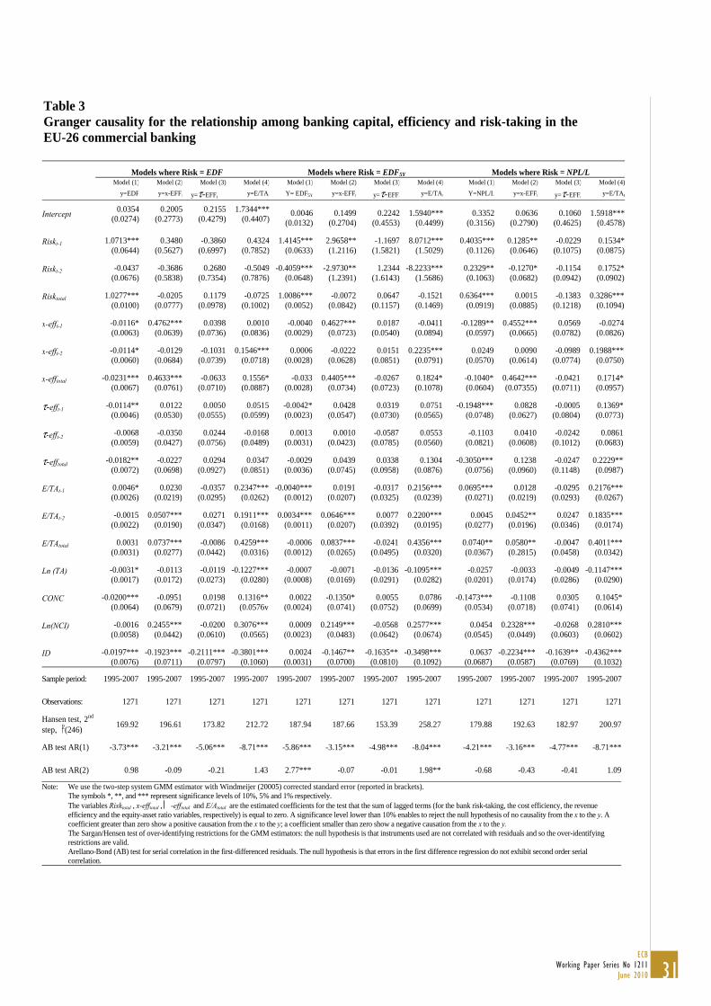
6. Results
We report the results from models (1)-(4) using two lags on equity capital, cost efficiency,
revenue efficiency and bank risk in table 3, where bank risk is measured using EDF (i.e. the
1-year ahead expected default frequency), the EDF5Y (i.e. the 5-year ahead expected default
frequency) and the NPL/L (i.e. the ratio of non-performing to total loans).
<<INSERT TABLE 3 >>
Cost (x-eff) and revenue (τ-eff) efficiencies are found to negatively Granger-cause bank’s
EDF (i.e. y=EDF in table 3). Our results show that a decline in the sum of the lagged
efficiency coefficients, i.e. the ‘long-run effect’ (for both cost and revenue efficiency,
respectively) temporally precede an increase in the EDF. This suggests that reductions in
bank efficiency (either cost or revenue) Granger cause a higher probability of default – this
confirms the “bad management” hypothesis and is in-line with the earlier findings of Berger
and De Young (1997), Kwan and Eisenbeis (1997) and Williams (2004)
We also find a negative statistically significant (at the 1% level) link between EDF
and the concentration index showing that bank risks are lower in more concentrated markets
(i.e. less concentrated – possibly more competitive – banking systems might be less stable in
the long-run in line with Boyd and Nicolo, 2003). These conclusions are also supported when
an accounting measure is used to assess bank risk. In the NPL/L model (i.e. y=NPL/L in table
3): cost and revenue efficiency declines temporally precede NPL increases. There is also a
negative link between the NPL/L ratio and the concentration index. When bank risk is
measured using the EDF5Y (so over a long-term horizon), we find no relationship between
industry structure and risk suggesting that effects get blurred in terms of long-run risk
expectations.

20ECBWorking Paper Series No 1211June 2010
We show that the capital ratio (E/TA) is found to positively Granger-cause cost
efficiencies (x-eff) (statistically significant at 5% or less) in all the model (2) estimations (i.e.
y=x-eff in table 3). Namely, an increase in the sum of the lagged capital ratio coefficients
temporally precede cost efficiency increases although there is no impact on risk. This
suggests that moral hazard incentives appear to fall as bank capital increases and these banks
are more likely to reduce costs (e.g. shareholder may be more active in controlling bank costs
or capital allocation) than thinly capitalised banks. These conclusions are independent from
the bank risk measure adopted in estimating model (2): namely, the long-run positive
causation effect between capital and cost efficiency is found in all models using different
definitions of bank risk (i.e. EDF, EDF5Y, NPL/L). We also find a positive statistically
significant (at the 1% level) link between cost efficiency and the number of credit institutions
(NCI) suggesting that cost efficiency levels are positively linked to the number of competitors
in the market (supporting the view that competition makes banks more cost effective). We
also find a negative statistically significant (at the 5% level or less) link between cost
efficiency and income diversification (ID) suggesting that more specialised banks benefit
from scale and learning economies that enable them to reduce costs more than their
diversified counterparts. These conclusions are also independent from the bank risk measure
adopted.
We also show that the cost efficiency indicator (x-eff) is found to positively Granger-
cause bank’s capital (E/TA) (statistically significant at 10% or less) in all the models (4)
estimations (i.e. y=E/TA in table 3). Increases in the sum of the lagged cost efficiency
coefficients temporally precede equity ratio increases and the result holds for all bank risk
measures (i.e. EDF, EDF5Y, NPL/L) used in estimating model (4). This finding is consistent
with Berger and DeYoung (1997) and Williams (2004) where short-term cost efficiency
gains (driven by reducing loan underwriting, monitoring and control costs) would feed
21ECB
Working Paper Series No 1211June 2010
through into higher capital. This is probably because more efficient banks have higher
earnings which Granger-cause increases in capital.
We also find a positive statistically significant (at the 1% level) link between the
capital ratio and the number of credit institutions (NCI) tentatively suggesting that high
capital levels are positively linked to the number of competitors in the market (so supporting
the view that bank competition might encourage higher equity capital levels).
Surprisingly and unlike most of the previous literature we find no strong causal
relationship between capital and risk (when measured using EDF or EDF5Y) for our period of
study. There is however evidence of positive bi-directional Granger causality when NPL/L is
our risk measure. This suggests that capital is more likely to be related to past credit risks
than broader-based (future) banking risks.
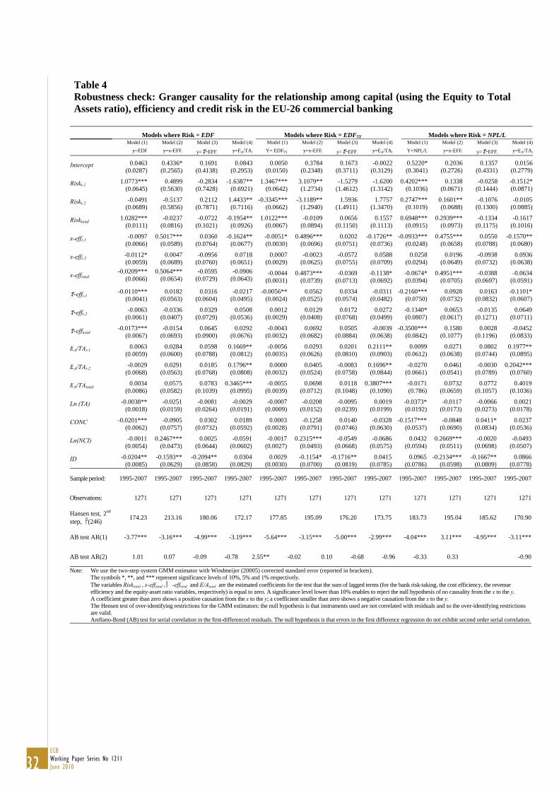
7. Robustness tests
In order to confirm the validity of the aforementioned findings, we conducted a number of
robustness checks. Firstly, we calculate the equity ratio in a standard accounting way (EA/TA)
by focussing on the book value of total equity (rather than the Basel Committee capital
definition) and we re-estimate models (1) to (4). As in table 3, table 4 reports all the results
obtained from estimating models (1)-(4) using the three different measures of bank risk (i.e.
the EDF, the EDF5Y and the NPL/L). While we are able to confirm that cost efficiency (x-eff)
and revenue efficiency (τ-eff) negatively Granger-cause bank’s EDF and NPL/L (statistically
significant at 10% or less), in the estimation of model (1) we cannot confirm our previous
results concerning capital ratios. We find no evidence of Granger-causation between our
narrow measure of capital (EA/TA) and bank cost efficiencies. This suggests that the use of
supplementary capital items such as subordinated debt and hybrid capital instruments
(commonly used by European banks) may influence capital cost efficiency relationships. As

22ECBWorking Paper Series No 1211June 2010
in our previous results we find little relationship between equity capital and risk apart from
evidence that EDF negatively causes equity capital – higher long-run risk seems to Granger
cause reductions in equity capital over time although we find no such relationship for our
other risk measures.
<<INSERT TABLE 4 >>
Secondly, we also estimate profit efficiency (rather than cost and revenue efficiency
as noted above) and re-estimate models (1) to (4). Our results (table 5) show that profit
efficiency (π-eff) is found to positively Granger-cause bank’s capital (E/TA) (statistically
significant at 10% or less) in all the model (4) estimations (i.e. y=E/TA in table 5). This result
is consistent with the positive causation between cost efficiency and the capital-asset ratio.
We also find evidence that profit efficiency negatively Granger-causes (at the 10%
confidence level) bank’s EDF or NPL/L in the model (1) estimations. As in Table 3 we also
find a bi-directional causal relationship between capital and NPL/L.
<<INSERT TABLE 5 >>
Thirdly, we re-estimate equations (1)-(4) positing a AR(4) lag structure for bank risk, capital
and efficiency. This change has substantial effects on our sample composition by reducing the
number of bank observations from 1,987 to 667. As shown in table 6, the AR(4) specification
cannot be safely assumed since longer lags may be weak instruments. As expected, test
statistics are found to be insignificant at three and four lags and, overall, we find little
evidence to support the claim that causal relationships exist (in the long run) beyond a single
or two-lag (i.e. two years) period.
23ECB
Working Paper Series No 1211June 2010
<<INSERT TABLE 6 >>
8. Conclusions
We assess the inter-temporal relationships among bank efficiency, capital and risk for the
European commercial banking industry. We build on previous work using Granger-causality
methods (Berger and De Young 1997, Williams 2004) in a panel data framework. Our model
delves into the relationships by including several definitions of bank efficiency (i.e. cost,
revenue and profit efficiency scores), risk (i.e. non-performing loans and probability of
default) and capital (i.e. core equity and total capital).
In general, our results show that subdued bank efficiency (cost or revenue) Granger
causes risk supporting the “bad management” and the “efficiency version of the moral
hazard” hypotheses. We also show that increases in bank capital precede cost efficiency
improvements suggesting that moral hazard incentives appear to fall as bank capital
increases. Better capitalized banks are more likely to reduce their costs compared to their
thinly capitalized counterparts. Cost (and profit) efficiencies are also found to positively
Granger-cause bank capital. In other words more efficient banks seem to eventually become
better capitalized and higher capital levels also tend to have a positive effect on efficiency
levels.
We find only limited evidence of relationships between capital and risk in line with
the moral hazard hypothesis. The main finding seems to be a bi-directional causal link
between capital and our accounting measure of risk (NPL/L). There is little evidence of any
strong causal link between capital (total capital or equity capital) and our market-based bank
risk indicators.
Overall we believe our results to be particularly interesting from a prudential

24ECBWorking Paper Series No 1211June 2010
supervisory perspective. The findings showing that lower efficiency scores (either cost or
revenue) suggest greater future risks and efficiency improvements tend to shore up banks’
capital positions. Our findings also emphasize the importance of attaining long-term
efficiency gains to support financial stability objectives.
25ECB
Working Paper Series No 1211June 2010
References Altunbas, Y., Chakravarty, S., 2001. Frontier cost functions and bank efficiency. Economic Letters 72, 233-240.
Altunbas, Y. Carbo, S., Gardener, E.P.M., Molyneux, P., 2007. Examining the relationships between capital, risk and efficiency in European banking. European Financial Management 13, 49-70. Aly, H.Y., Grabowski, R., Pasurka, C., Rangan, N., 1990. Technical, scale and allocative effciencies in US banking: an empirical investigation, Review of Economics and Statistics 72, 211-218.
Amato, J.D., Swanson, N.R., 2001. The real-time predictive content of money for output. Journal of Monetary Economics 48, 3-24.
Arellano, M., 1989. A note on the Anderson-Hsiao estimator for panel data. Economic Letters 31, 337-341.
Arellano, M., Bond, S.R., 1991. Some tests of specification for panel data: Monte Carlo evidence and an application to employment equations. Review of Economic Studies 58, 277-297.
Arellano, M., Bover, O., 1995. Another look at the instrumental variable estimation of error-components models. Journal of Econometrics 68, 29-51.
Assenmacher-Wesche, K., Gerlach, S., 2008. Interpreting euro area inflation at high and low frequencies. European Economic Review 52, 964-986.
Ayuso, J., Perez, D., Saurina, J. (2004). Are capital buffers pro-cyclical? Evidence from Spanish panel data, Journal of Financial Intermediation 13, 249-264.
Bajo-Rubio, O., Sosvilla-Rivero, S., Fernández-Rodríguez. F., 2001. Asymmetry in the EMS: New evidence based on non-linear forecasts. European Economic Review 45, 451-473.
Barrios, V.E.J., Blanco, J., 2003. The effectiveness of bank capital adequacy regulations: an empirical approach. Journal of Banking and Finance 27, 1935-1958.
Battese, G.E., Coelli, T.J., 1995. A model for technical inefficiency effects in a stochastic frontier production function for panel data. Empirical Economics 20, 325-32.
Beccalli, E., 2007. Does IT investment improve bank performance? Evidence from Europe. Journal of Banking and Finance 31, 2205-2230.
Berger, A.N., Bonaccorsi di Patti, E., 2006. Capital structure and firm performance: A new approach to testing agency theory and an application to the banking industry. Journal of Banking and Finance 30, 1065-1102.
Berger, A.N., Humphrey, D. B., 1992. Measurement and efficiency issues in commercial banking, in Output Measurement in the Service Sectors, Zvi Griliches eds. The University of Chicago Press, 245-279.
Berger, A.N., Mester, L.J., 1997. Inside the black box: What explains differences in the efficiency of financial institutions. Journal of Banking and Finance 21, 895-947.
Berger, A.N., Herring, R.J., Szego, G.P., 1995. The role of capital in financial institutions. Journal of Banking and Finance 19, 393-430.
26ECBWorking Paper Series No 1211June 2010
Berger, A.N., De Young R., 1997. Problem loans and cost efficiency in commercial banking. Journal of Banking and Finance 21, 849-870.
Besanko, D., Kanatas, G., 1996. The regulation of bank capital: Do capital standards promote bank safety? Journal of Financial Intermediation 5, 160-183.
Blundell, R., Bond, S., 1998. Initial conditions and moment restrictions in dynamic panel data models. Journal of Econometrics 87, 115-143.
Blundell, R., Bond, S., Windmeijer, F., 2000. Estimation in dynamic panel data models: Improving on the performance of the standard GMM estimator. Advances in Econometrics 15, 53–91.
Bhattacharya, S., Boot, A.W.A, Thakor, A.V., 1998. The economics of bank regulation. Journal of Money, Credit and Banking 30, 745-770. Bos, J., Schmiedel, H., 2007. Is there a single frontier in a single European banking market? Journal of Banking and Finance 31, 2081-2102.
Bos, J., Koetter, M., Kolari, J., Kool, C., 2009. Effects of heterogeneity on bank efficiency scores. European Journal of Operational Research 19, 251-261.
Boyd, J.H., Nicolo, G.D., 2003. The theory of bank risk taking and competition revisited. Journal of Finance 60, 1329-1343.
Carletti, E., Hartmann, P., 2002. Competition and stability: What's special about banking? Working Paper, European Central Bank 146.
Casu, B., Girardone, C., 2009. Testing the relationship between competition and efficiency in banking: A panel data analysis. Economics Letters 105, 134-137.
Cihak, M., Schaeck, K.. Wolfe, S., 2009. Are competitive banking systems more stable? Journal of Money, Credit, and Banking 41, 711-734.
Dahl, D., Shrieves, R.E., 1990. The impact of regulation on bank equity infusions. Journal of Banking and Finance 14, 1209-1228.
Demsetz, R.S., Saindenberg, M. R., Strahan P.E., 1996. Banks with something to lose: The disciplinary role of franchise value, Federal Reserve Bank of New York Economic Policy Review 2, 1-14.
Diamond, D., Rajan R. A., 2000. Theory of bank capital. Journal of Finance 55, 2431-65.
Dietsch, M., Lozano-Vives, A., 2000. How the environment determines banking efficiency: A comparison between French and Spanish industries. Journal of Banking and Finance 24, 985-1004.
Dwyer, D., Qu, S., 2007. EDF™ 8.0 Model Enhancements, Moody’s KMV.
Ediz, T., Michael, I., Perraudin, W., 1998. The impact of capital requirements on U.K. bank behaviour. Federal Reserve Bank of New York Economic Policy Review, October.
European Central Bank, 2010. Financial Integration in Europe, April.
Fiordelisi, F., Molyneux, P., 2010. The determinants of shareholder value in European Banking. Journal of Banking and Finance 34, 1189-1200.
Frame, S.W., Coelli, T., 2001. U.S. financial services consolidation: The case of corporate credit unions. Review of Industrial Organization 18, 229-242.
27ECB
Working Paper Series No 1211June 2010
Freixas, X., Gabillon, E., 1998. Optimal regulation of a fully insured deposit banking system. Journal of Regulatory Economics 16, 111-34.
Freixas, X., Rochet, J., 1997. Microeconomics of Banking. MIT press, Cambridge.
Friedman, M., 1962. Price Theory: A Provisional Text. Chicago, Aldine.
Garlappi, L., Uppal, R., Wang, T., 2007. Portfolio selection with parameter and model uncertainty: A multi-prior approach. The Review of Financial Studies 20, 1, 41-81.
Granger, C.W.J., 1969. Investigating causal relations by econometric models and cross-spectral methods. Econometrica 37, 424-438.
Goddard, J., Molyneux, P., Wilson, J.O.S., Tavakoli, M., 2007. European Banking: An Overview. Journal of Banking and Finance 31, 1911–35.
Gorton, G., Rosen, R., 1995. Corporate control, portfolio choice and the decline of banking. Journal of Finance 50, 1377-1420.
Hancock, D., 1986. A model of the financial firm with imperfect asset and deposit elasticities. Journal of Banking and Finance 10, 37-54.
Haldane, A. G., Alessandri, P., 2009. Banking on the state. Presentation delivered at the Federal Reserve Bank of Chicago twelfth annual International Banking Conference on “The International Financial Crisis: Have the Rules of Finance Changed?”, Chicago, 25 September 2009.
Gropp, R., Heider, F., 2010. The determinants of bank capital structure. Review of Finance, forthcoming.
Hellmann, T. F., Murdock, K. C., Stiglitz, J.E., 2000. Liberalization, moral hazard in banking, and prudential regulation: Are capital requirements enough? American Economic Review 90, 147-65.
Hughes, J.P., Mester, L.J, 1998. Bank capitalization and cost: Evidence of scale economies in risk management and signalling. The Review of Economics and Statistics 80, 314-325.
Hughes, J.P., Mester, L.J., 2009. Efficiency in banking: Theory, practice and evidence. In Berger, A.N., Molyneux, P., Wilson, J.O.S (Eds.). Oxford Handbook of Banking. Oxford University Press, Chapter 18.
Hurlin, C., Venet, B., 2001. Granger causality tests in panel data models with fixed coefficients. Working Paper, Eurisco University of Paris Dauphine 2001-09.
Jackson, P., 1999. Capital requirements and bank behaviour: The impact of the Basle accord. Basle Committee on Banking Supervision Working Papers 1.
Jaeger, D.A., Paserman, M.D., 2008. The cycle of violence? An empirical analysis of fatalities in the Palestinian-Israeli conflict. American Economic Review 98, 1591-1604.
Jeitschko, T.D., Jeung, S.D., 2005. Incentives for risk-taking in banking – A unified approach. Journal of Banking and Finance 29, pp. 759-777.
Kealhofer, S., 2003. Quantifying credit risk I: Default prediction. Financial Analysts Journal 59, 1, 30-44.
Kwan, S. Eisenbeis, R., 1997. Bank risk, capitalization and operating efficiency. Journal of Financial Services Research 12, 117-131.
Lepetit, L., Nys, E., Rous, P., Tarazi, A., 2008. Bank income structure and risk: An empirical analysis of European banks. Journal of Banking and Finance 32, 1452–1467.

28ECBWorking Paper Series No 1211June 2010
Levine, R., Loayza, N., Beck, T., 2000. Financial intermediation and growth: Causality and causes. Journal of Monetary Economics, 46, 31-77.
Marcus, A.J., 1983. The bank capital decision: A time series-cross section analysis. Journal of Finance 38, 1216-1232.
Marshall, D. and E.S. Precott., 2001. Bank capital regulation with and without state contingent penalties. Carnegie-Rochester Conferences Series 54, 139-84.
Matutes C., Vives, X., 2000. Imperfect competition, risk taking, and regulation in banking. European Economic Review 44, 1-34.
Mayne, L.S., 1972. Supervisory influence on bank capital. Journal of Finance 27, 637-651.
Memmel, C., Raupach, P., 2010. How do banks adjust their capital ratios? Journal of Financial Intermediation, Forthcoming.
Merton, R.C., 1974. On the pricing of corporate debt: The risk structure of interest rates. Journal of Finance 29, 449–470.
Ngo, P.T.H., 2008. Capital-Risk decisions and profitability in banking: Regulatory versus economic capital. 21st Australasian Finance and Banking Conference 2008, Working Paper Series.
Pastor, J. M., Serrano, L., 2005. Efficiency, endogenous and exogenous credit risk in the banking systems of the Euro area, Applied Financial Economics, 15, 631-649.
Peltzman, S., 1970. Capital investment in commercial banking and its relationship to portfolio regulation. Journal of Political Economy, 1-26.
Peura, S., Keppo, J., 2006. Optimal bank capital with costly recapitalization. Journal of Business 79, 2162-2201.
Repullo, R., 2004. Capital requirement, market power, and risk-taking in banking. Journal of Financial Intermediation 13, 156-182.
Salas, V., Saurina, J., 2003. Deregulation, market power and risk behaviour in Spanish banks. European Economic Review 47, 1061-1075.
Santos, J.A.C., 1999. Bank capital regulation in contemporary banking theory: A review of the literature. BIS Working Paper 90.
Sathye, M., 2001. X-efficiency in Australian banking: an empirical investigation. Journal of Banking and Finance 25, 613-630.
Shrieves, R.E., Dahl, D., 1992. The relationship between risk and capital in commercial banks. Journal of Banking and Finance 16, 439-457.
Vives, X., 2000. Lessons from European banking liberalization and integration, The Internationalization of Financial Services: Issues and Lessons for Developing Countries. Kluwer Law International.
Wall, L.D., Peterson, D.R., 1987. The effects of capital adequacy guidelines on large bank holding companies. Journal of Banking and Finance 11, 581-600.
Williams, J., 2004. Determining management behaviour in European banking. Journal of Banking and Finance 28, 2427-2460.
Windmeijer, F., 2005. A finite sample correction for the variance of linear efficient two-step GMM estimators. Journal of Econometrics 126, 25-51.

29ECB
Working Paper Series No 1211June 2010
Table 1 Variables description
Variables Symbol Description
Cost Efficiency x-eff Estimated using Stochastic Frontier analysis.(*)
Revenue Efficiency τ-eff Estimated using Stochastic Frontier analysis.(*)
Profit Efficiency π-eff Estimated using Stochastic Frontier analysis.(*)
Non Performing Loans NPL/L Non-performing loans over the total gross value of total bank loans.(1)
1-Year Ahead Expected Default Frequency™
EDF Probability that a company (bank) will default within a year. (2)
5-Years Ahead Expected Default Frequency™
EDF5Y Cumulative probability that a company (bank) will default within 5 years.(3)
Capital to Asset Ratio E/TA Value of total equity divided by total assets. Equity capital is measured focusing on the Basel Committee definition of capital by summing total equity, retained earnings, general banking risk reserves, other equity reserves, hybrid capital instruments and subordinated debts.(1)
Book value of Capital to Asset Ratio EA/TA Total equity divided by total assets. Equity capital is measured by the book
value of total equity.(1)
Income Diversification ID Net non-interest income to net operating income.(1)
Bank Asset Size BAS BAS is the Euro value of its total assets.(1)
Domestic Banking Industry Concentration CONC Herfindahl-Hirschman Index.(4)
Number of Credit Institutions NCI NCI is the number of credit institutions.(5)
Interest Rate IR 3-month money market interest rate.(6)
GDP Per-capita Ln(GDPP) Natural logarithm of the domestic GDP (in Euro) divided by the number of inhabitants.(6)
GDP Annual Growth Rate GDPG Domestic GDP growth rate between two consecutive years.(6)
Population Density Ln(POPD) Natural logarithm of the number of inhabitants per Km.2 (6)
* More detail for the estimation procedures are provided in the Annex. 1) Source of data: Bankscope. 2) Source of data: KMV-Moody’s. 3) Source of data: KMV-Moody’s. 4) Source of data: ECB, EU Banking Structures, reports. 5) Source of data: ECB, MFI statistical reports. 6) Source of data: The United Nations.

30ECBWorking Paper Series No 1211June 2010
,
Table 2 The evolution of the main variables (Mean values) used to analyse the sample of EU-26 area banks over the period 1995-2007 (1,987 year-observations) x-EFF τ-EFF π-EFF EDF EDF5Y NPL/L E/TA ID BAS(*)
1995 0.5148 0.6095 0.5200 0.0031 0.0049 0.0334 0.0865 0.1285 327.9901996 0.4801 0.5967 0.4954 0.0042 0.0043 0.0366 0.0769 0.1433 307.2861997 0.4899 0.6218 0.5247 0.0038 0.0049 0.0354 0.0697 0.1656 403.6181998 0.4785 0.6267 0.5211 0.0042 0.0043 0.0356 0.0668 0.1686 377.7091999 0.4726 0.6336 0.5339 0.0047 0.0043 0.0343 0.0685 0.1800 336.3662000 0.4771 0.6309 0.5320 0.0042 0.0052 0.0343 0.0687 0.1916 428.3672001 0.4591 0.6304 0.5336 0.0073 0.0060 0.0354 0.0699 0.2002 343.2932002 0.4520 0.6355 0.5500 0.0084 0.0068 0.0364 0.0689 0.2068 345.3342003 0.4458 0.6341 0.5436 0.0101 0.0090 0.0355 0.0702 0.2047 377.3292004 0.4215 0.6254 0.5333 0.0070 0.0061 0.0341 0.0706 0.2248 552.3972005 0.4238 0.6285 0.5343 0.0058 0.0077 0.0333 0.0748 0.2228 708.1292006 0.4188 0.6204 0.5284 0.0087 0.0083 0.0328 0.0747 0.2107 792.8082007 0.4170 0.6529 0.5333 0.0042 0.0074 0.0301 0.0763 0.1860 902.372Total 0.4446 0.6311 0.5342 0.0067 0.0067 0.0342 0.0715 0.2014 579.947(*) Values are in Euro millions
31ECB
Working Paper Series No 1211June 2010
Table 3 Granger causality for the relationship among banking capital, efficiency and risk-taking in the EU-26 commercial banking
Models where Risk = EDF Models where Risk = EDF5Y Models where Risk = NPL/L Model (1) Model (2) Model (3) Model (4) Model (1) Model (2) Model (3) Model (4) Model (1) Model (2) Model (3) Model (4)
y=EDF y=x-EFFt y=τ-EFFt y=E/TAt Y= EDF5Y y=x-EFFt y=τ-EFFt y=E/TAt Y=NPL/L y=x-EFFt y=τ-EFFt y=E/TAt
Intercept 0.0354(0.0274)
0.2005(0.2773)
0.2155(0.4279)
1.7344***(0.4407)
0.0046(0.0132)
0.1499(0.2704)
0.2242(0.4553)
1.5940***(0.4499)
0.3352(0.3156)
0.0636(0.2790)
0.1060(0.4625)
1.5918***(0.4578)
Riskt-1 1.0713***(0.0644)
0.3480(0.5627)
-0.3860(0.6997)
0.4324(0.7852)
1.4145***(0.0633)
2.9658**(1.2116)
-1.1697(1.5821)
8.0712***(1.5029)
0.4035***(0.1126)
0.1285**(0.0646)
-0.0229(0.1075)
0.1534*(0.0875)
Riskt-2 -0.0437(0.0676)
-0.3686(0.5838)
0.2680(0.7354)
-0.5049(0.7876)
-0.4059***(0.0648)
-2.9730**(1.2391)
1.2344(1.6143)
-8.2233***(1.5686)
0.2329**(0.1063)
-0.1270*(0.0682)
-0.1154(0.0942)
0.1752*(0.0902)
Risktotal 1.0277***(0.0100)
-0.0205(0.0777)
0.1179(0.0978)
-0.0725(0.1002)
1.0086***(0.0052)
-0.0072(0.0842)
0.0647(0.1157)
-0.1521(0.1469)
0.6364***(0.0919)
0.0015(0.0885)
-0.1383(0.1218)
0.3286***(0.1094)
x-efft-1 -0.0116*(0.0063)
0.4762***(0.0639)
0.0398(0.0736)
0.0010(0.0836)
-0.0040(0.0029)
0.4627***(0.0723)
0.0187(0.0540)
-0.0411(0.0894)
-0.1289**(0.0597)
0.4552***(0.0665)
0.0569(0.0782)
-0.0274(0.0826)
x-efft-2 -0.0114*(0.0060)
-0.0129(0.0684)
-0.1031(0.0739)
0.1546***(0.0718)
0.0006(0.0028)
-0.0222(0.0628)
0.0151(0.0851)
0.2235***(0.0791)
0.0249(0.0570)
0.0090(0.0614)
-0.0989(0.0774)
0.1988***(0.0750)
x-efftotal -0.0231***(0.0067)
0.4633***(0.0761)
-0.0633(0.0710)
0.1556*(0.0887)
-0.033(0.0028)
0.4405***(0.0734)
-0.0267(0.0723)
0.1824*(0.1078)
-0.1040*(0.0604)
0.4642***(0.07355)
-0.0421(0.0711)
0.1714*(0.0957)
τ-efft-1 -0.0114**(0.0046)
0.0122(0.0530)
0.0050(0.0555)
0.0515(0.0599)
-0.0042*(0.0023)
0.0428(0.0547)
0.0319(0.0730)
0.0751(0.0565)
-0.1948***(0.0748)
0.0828(0.0627)
-0.0005(0.0804)
0.1369*(0.0773)
τ-efft-2 -0.0068(0.0059)
-0.0350(0.0427)
0.0244(0.0756)
-0.0168(0.0489)
0.0013(0.0031)
0.0010(0.0423)
-0.0587(0.0785)
0.0553(0.0560)
-0.1103(0.0821)
0.0410(0.0608)
-0.0242(0.1012)
0.0861(0.0683)
τ-efftotal -0.0182**(0.0072)
-0.0227(0.0698)
0.0294(0.0927)
0.0347(0.0851)
-0.0029(0.0036)
0.0439(0.0745)
0.0338(0.0958)
0.1304(0.0876)
-0.3050***(0.0756)
0.1238(0.0960)
-0.0247(0.1148)
0.2229**(0.0987)
E/TAt-1 0.0046*(0.0026)
0.0230(0.0219)
-0.0357(0.0295)
0.2347***(0.0262)
-0.0040***(0.0012)
0.0191(0.0207)
-0.0317(0.0325)
0.2156***(0.0239)
0.0695***(0.0271)
0.0128(0.0219)
-0.0295(0.0293)
0.2176***(0.0267)
E/TAt-2 -0.0015(0.0022)
0.0507***(0.0190)
0.0271(0.0347)
0.1911***(0.0168)
0.0034***(0.0011)
0.0646***(0.0207)
0.0077(0.0392)
0.2200***(0.0195)
0.0045(0.0277)
0.0452**(0.0196)
0.0247(0.0346)
0.1835***(0.0174)
E/TAtotal 0.0031(0.0031)
0.0737***(0.0277)
-0.0086(0.0442)
0.4259***(0.0316)
-0.0006(0.0012)
0.0837***(0.0265)
-0.0241(0.0495)
0.4356***(0.0320)
0.0740**(0.0367)
0.0580**(0.2815)
-0.0047(0.0458)
0.4011***(0.0342)
Ln (TA) -0.0031*(0.0017)
-0.0113(0.0172)
-0.0119(0.0273)
-0.1227***(0.0280)
-0.0007(0.0008)
-0.0071(0.0169)
-0.0136(0.0291)
-0.1095***(0.0282)
-0.0257(0.0201)
-0.0033(0.0174)
-0.0049(0.0286)
-0.1147***(0.0290)
CONC -0.0200***(0.0064)
-0.0951(0.0679)
0.0198(0.0721)
0.1316**(0.0576v
0.0022(0.0024)
-0.1350*(0.0741)
0.0055(0.0752)
0.0786(0.0699)
-0.1473***(0.0534)
-0.1108(0.0718)
0.0305(0.0741)
0.1045*(0.0614)
Ln(NCI) -0.0016(0.0058)
0.2455***(0.0442)
-0.0200(0.0610)
0.3076***(0.0565)
0.0009(0.0023)
0.2149***(0.0483)
-0.0568(0.0642)
0.2577***(0.0674)
0.0454(0.0545)
0.2328***(0.0449)
-0.0268(0.0603)
0.2810***(0.0602)
ID -0.0197***(0.0076)
-0.1923***(0.0711)
-0.2111***(0.0797)
-0.3801***(0.1060)
0.0024(0.0031)
-0.1467**(0.0700)
-0.1635**(0.0810)
-0.3498***(0.1092)
0.0637(0.0687)
-0.2234***(0.0587)
-0.1639**(0.0769)
-0.4362***(0.1032)
Sample period: 1995-2007 1995-2007 1995-2007 1995-2007 1995-2007 1995-2007 1995-2007 1995-2007 1995-2007 1995-2007 1995-2007 1995-2007
Observations: 1271 1271 1271 1271 1271 1271 1271 1271 1271 1271 1271 1271
Hansen test, 2nd step, ⎟2(246) 169.92 196.61 173.82 212.72 187.94 187.66 153.39 258.27 179.88 192.63 182.97 200.97
AB test AR(1) -3.73*** -3.21*** -5.06*** -8.71*** -5.86*** -3.15*** -4.98*** -8.04*** -4.21*** -3.16*** -4.77*** -8.71***
AB test AR(2) 0.98 -0.09 -0.21 1.43 2.77*** -0.07 -0.01 1.98** -0.68 -0.43 -0.41 1.09
Note: We use the two-step system GMM estimator with Windmeijer (20005) corrected standard error (reported in brackets). The symbols *, **, and *** represent significance levels of 10%, 5% and 1% respectively. The variables Risktotal , x-efftotal , ⎮ -efftotal and E/Atotal are the estimated coefficients for the test that the sum of lagged terms (for the bank risk-taking, the cost efficiency, the revenue efficiency and the equity-asset ratio variables, respectively) is equal to zero. A significance level lower than 10% enables to reject the null hypothesis of no causality from the x to the y. A coefficient greater than zero show a positive causation from the x to the y; a coefficient smaller than zero show a negative causation from the x to the y.
The Sargan/Hensen test of over-identifying restrictions for the GMM estimators: the null hypothesis is that instruments used are not correlated with residuals and so the over-identifying restrictions are valid. Arellano-Bond (AB) test for serial correlation in the first-differenced residuals. The null hypothesis is that errors in the first difference regression do not exhibit second order serial correlation.
32ECBWorking Paper Series No 1211June 2010
Table 4 Robustness check: Granger causality for the relationship among capital (using the Equity to Total Assets ratio), efficiency and credit risk in the EU-26 commercial banking
Models where Risk = EDF Models where Risk = EDF5Y Models where Risk = NPL/L
Model (1) Model (2) Model (3) Model (4) Model (1) Model (2) Model (3) Model (4) Model (1) Model (2) Model (3) Model (4)
y=EDF y=x-EFFt y=τ-EFFt y=EA/TAt Y= EDF5Y y=x-EFFt y=τ-EFFt y=EA/TAt Y=NPL/L y=x-EFFt y=τ-EFFt y=EA/TAt
Intercept 0.0463(0.0287)
0.4336* (0.2565)
0.1691(0.4138)
0.0843(0.2953)
0.0050(0.0150)
0.3784(0.2348)
0.1673(0.3711)
-0.0022(0.3129)
0.5220*(0.3041)
0.2036(0.2726)
0.1357(0.4331)
0.0156(0.2779)
Riskt-1 1.0773***
(0.0645)0.4899
(0.5630) -0.2834
(0.7428)-1.6387**
(0.6921)1.3467***
(0.0642)3.1079**(1.2734)
-1.5279(1.4612)
-1.6200(1.3142)
0.4202***(0.1036)
0.1338(0.0671)
-0.0258(0.1444)
-0.1512*(0.0871)
Riskt-2 -0.0491(0.0689)
-0.5137 (0.5856)
0.2112(0.7871)
1.4433**(0.7116)
-0.3345***(0.0662)
-3.1189**(1.2940)
1.5936(1.4911)
1.7757(1.3470)
0.2747***(0.1019)
0.1601**(0.0688)
-0.1076(0.1300)
-0.0105(0.0885)
Risktotal 1.0282***
(0.0111)-0.0237
(0.0816) -0.0722
(0.1021)-0.1954**
(0.0926)1.0122***
(0.0067)-0.0109
(0.0894)0.0656
(0.1150)0.1557
(0.1113)0.6948***
(0.0915)0.2939***
(0.0973)-0.1334
(0.1175)-0.1617
(0.1016)
x-efft-1 -0.0097
(0.0066)0.5017***
(0.0589) 0.0360
(0.0764)-0.1624**
(0.0677)-0.0051*(0.0030)
0.4896***(0.0696)
0.0202(0.0751)
-0.1726**(0.0736)
-0.0933***(0.0248)
0.4755***(0.0658)
0.0550(0.0788)
-0.1570**(0.0680)
x-efft-2 -0.0112*(0.0059)
0.0047 (0.0689)
-0.0956(0.0760)
0.0718(0.0651)
0.0007(0.0029)
-0.0023(0.0625)
-0.0572(0.0755)
0.0588(0.0709)
0.0258(0.0294)
0.0196(0.0649)
-0.0938(0.0732)
0.0936(0.0638)
x-efftotal -0.0209***
(0.0066)0.5064***
(0.0654) -0.0595
(0.0729)-0.0906
(0.0643)-0.0044
(0.0031)0.4873***
(0.0739)-0.0369
(0.0713)-0.1138*(0.0692)
-0.0674*(0.0394)
0.4951***(0.0705)
-0.0388(0.0697)
-0.0634(0.0591)
τ-efft-1 -0.0110***
(0.0041)0.0182
(0.0563) 0.0316
(0.0604)-0.0217
(0.0495)-0.0056**
(0.0024)0.0562
(0.0525)0.0334
(0.0574)-0.0311
(0.0482)-0.2160***
(0.0750)0.0928
(0.0732)0.0163
(0.0832)-0.1101*(0.0607)
τ-efft-2 -0.0063
(0.0061)-0.0336
(0.0407) 0.0329
(0.0729)0.0508
(0.0536)0.0012
(0.0029)0.0129
(0.0408)0.0172
(0.0768)0.0272
(0.0499)-0.1340*(0.0807)
0.0653(0.0617)
-0.0135(0.1271)
0.0649(0.0711)
τ-efftotal -0.0173***
(0.0067)-0.0154
(0.0693) 0.0645
(0.0900)0.0292
(0.0676)-0.0043
(0.0032)0.0692
(0.0682)0.0505
(0.0884)-0.0039
(0.0638)-0.3500***
(0.0842)0.1580
(0.1077)0.0028
(0.1196)-0.0452
(0.0833)
EA/TAt-1 0.0063
(0.0059)0.0284
(0.0600) 0.0598
(0.0788)0.1669**(0.0812)
-0.0056(0.0035)
0.0293(0.0626)
0.0201(0.0810)
0.2111**(0.0903)
0.0099(0.0612)
0.0271(0.0638)
0.0802(0.0744)
0.1977**(0.0895)
EA/TAt-2 -0.0029(0.0068)
0.0291 (0.0563)
0.0185(0.0768)
0.1796**(0.0808)
0.0000(0.0032)
0.0405(0.0524)
-0.0083(0.0758)
0.1696**(0.0844)
-0.0270(0.0661)
0.0461(0.0541)
-0.0030(0.0789)
0.2042***(0.0760)
EA/TAtotal 0.0034
(0.0086)0.0575
(0.0582) 0.0783
(0.1039)0.3465***
(0.0995)-0.0055
(0.0039)0.0698
(0.0712)0.0118
(0.1048)0.3807***
(0.1090)-0.0171(0.786)
0.0732(0.0659)
0.0772(0.1057)
0.4019(0.1036)
Ln (TA) -0.0038**(0.0018)
-0.0251 (0.0159)
-0.0081(0.0264)
-0.0029(0.0191)
-0.0007(0.0009)
-0.0208(0.0152)
-0.0095(0.0239)
0.0019(0.0199)
-0.0373*(0.0192)
-0.0117(0.0173)
-0.0066(0.0273)
0.0021(0.0178)
CONC -0.0201***(0.0062)
-0.0905 (0.0757)
0.0302(0.0732)
0.0189(0.0592)
0.0003(0.0028)
-0.1258(0.0791)
0.0140(0.0746)
-0.0328(0.0630)
-0.1517***(0.0537)
-0.0848(0.0690)
0.0411*(0.0834)
0.0237(0.0536)
Ln(NCI) -0.0011(0.0054)
0.2467*** (0.0473)
0.0025(0.0644)
-0.0591(0.0602)
-0.0017(0.0027)
0.2315***(0.0493)
-0.0549(0.0668)
-0.0686(0.0575)
0.0432(0.0594)
0.2669***(0.0511)
-0.0020(0.0698)
-0.0493(0.0507)
ID -0.0204**(0.0085)
-0.1593** (0.0629)
-0.2094**(0.0858)
0.0304(0.0829)
0.0029(0.0030)
-0.1154*(0.0700)
-0.1716**(0.0819)
0.0415(0.0785)
0.0965(0.0786)
-0.2134***(0.0598)
-0.1667**(0.0809)
0.0866(0.0778)
Sample period: 1995-2007 1995-2007 1995-2007 1995-2007 1995-2007 1995-2007 1995-2007 1995-2007 1995-2007 1995-2007 1995-2007 1995-2007
Observations: 1271 1271 1271 1271 1271 1271 1271 1271 1271 1271 1271 1271
Hansen test, 2nd step, ⎟2(246) 174.23 213.16 180.06 172.17 177.85 195.09 176.20 173.75 183.73 195.04 185.62 170.90
AB test AR(1) -3.77*** -3.16*** -4.99*** -3.19*** -5.64*** -3.15*** -5.00*** -2.99*** -4.04*** 3.11*** -4.95*** -3.11***
AB test AR(2) 1.01 0.07 -0.09 -0.78 2.55** -0.02 0.10 -0.68 -0.96 -0.33 0.33 -0.90
Note: We use the two-step system GMM estimator with Windmeijer (20005) corrected standard error (reported in brackets). The symbols *, **, and *** represent significance levels of 10%, 5% and 1% respectively. The variables Risktotal , x-efftotal , ⎮ -efftotal and E/Atotal are the estimated coefficients for the test that the sum of lagged terms (for the bank risk-taking, the cost efficiency, the revenue efficiency and the equity-asset ratio variables, respectively) is equal to zero. A significance level lower than 10% enables to reject the null hypothesis of no causality from the x to the y. A coefficient greater than zero shows a positive causation from the x to the y; a coefficient smaller than zero shows a negative causation from the x to the y.
The Hensen test of over-identifying restrictions for the GMM estimators: the null hypothesis is that instruments used are not correlated with residuals and so the over-identifying restrictions are valid. Arellano-Bond (AB) test for serial correlation in the first-differenced residuals. The null hypothesis is that errors in the first difference regression do not exhibit second order serial correlation.

33ECB
Working Paper Series No 1211June 2010
Table 5 Robustness check: Granger causality for the relationship among capital, efficiency (measured using profit efficiency) and credit risk in the EU-26 commercial banking
Models where Risk = EDF Models where Risk = EDF5Y Models where Risk = NPL/L
Model (1) Model (5) Model (4) Model (1) Model (5) Model (4) Model (1) Model (5) Model (4) y=EDF y= π-EFFt y=E/TAt Y= EDF5Y y= π-EFFt y=E/TAt Y=NPL/L y= π-EFFt y=E/TAt
Intercept 0.0277(0.0303)
0.3496(0.3298)
1.9096***(0.4106)
0.0044(0.0133)
0.1332(0.3336)
1.7495***(0.3806)
0.4153(0.3093)
0.4396(0.3370)
1.7975***(0.4003)
Riskt-1 1.1257***(0.0645)
0.4410(0.8324)
-0.2236(0.7518)
1.4040***(0.0620)
-1.3386(1.1907)
7.2335***(1.4169)
0.2656***(0.0735)
-0.1026(0.0671)
0.0483(0.0603)
Riskt-2 -0.0969(0.0677)
-0.5435(0.8491)
0.1493(0.7482)
-0.3963***(0.0634)
1.1822(1.2046)
-7.3504***(1.4837)
0.1955***(0.0723)
-0.1624**(0.0696)
0.0610(0.0755)
Risktotal 1.0287***(0.0103)
-0.1025(0.0675)
-0.0743(0.1030)
1.0007***(0.0052)
-0.1564*(0.848)
-0.1169(0.1389)
0.4611***(0.0853)
-0.2650***(0.0915)
0.1093*(0.0958)
π-efft-1 -0.0065(0.0079)
0.1919***(0.0590)
-0.0684(0.0738)
-0.0050*(0.0028)
0.1773***(0.0659)
-0.0687(0.0756)
-0.0803(0.0722)
0.1388**(0.0676)
-0.0764(0.0744)
π-efft-2 -0.0073(0.0049)
0.1613***(0.0509)
0.2773***(0.0660)
0.0000(0.0027)
0.1587***(0.0492)
0.2404***(0.0668)
-0.0530(0.0481)
0.0893(0.0648)
0.2478***(0.0740)
π-efftotal -0.0138*(0.0080)
0.3532***(0.0807)
0.2089**(0.0946)
-0.0051(0.0031)
0.3360***(0.0863)
0.1717*(0.0988)
-0.1333*(0.0803)
0.2280**(0.1014)
0.1714*(0.0984)
E/TAt-1 0.0020(0.0029)
0.0047(0.0284)
0.2309***(0.0246)
-0.0049***(0.0012)
0.0275(0.0269)
0.2188***(0.0218)
0.0728***(0.0269)
0.0117(0.0294)
0.2318***(0.0229)
E/TAt-2 -0.0044*(0.0023)
-0.0069(0.0254)
0.2118***(0.0161)
0.0032***(0.0011)
0.0031(0.0268)
0.2368***(0.0190)
0.0085(0.0261)
-0.0027(0.0248)
0.2104***(0.0159)
E/TAtotal -0.0024(0.0032)
-0.0022(0.0385)
0.4426***(0.0275)
-0.0017(0.0013)
0.0306(0.0371)
0.4555***(0.0275)
0.0813**(0.0334)
0.0090(0.0395)
0.04421***(0.0256)
Ln (TA) -0.0026(0.0019)
-0.0214(0.0212)
-0.1340***(0.0261)
-0.0007(0.0008)
-0.0095(0.0213)
-0.1196***(0.0239)
-0.0310*(0.0181)
-0.0277(0.0219)
-0.1271***(0.0252)
CONC -0.0163***(0.0064)
-0.0894*(0.0536)
0.0895(0.0567)
0.0026(0.0024)
-0.0356(0.0506)
0.0326(0.0629)
-0.1240**(0.0560)
-0.0984**(0.0474)
0.0870(0.0545)
Ln(NCI) -0.0058(0.0052)
-0.0727*(0.0418)
0.3329***(0.0592)
0.0002(0.0022)
-0.0455(0.0390)
0.2698***(0.0573)
0.0004(0.0487)
-0.0681*(0.0407)
0.3193***(0.0523)
ID -0.0168**(0.0085)
0.0469(0.0748)
-0.4113***(0.1105)
0.0034(0.0029)
0.0740(0.0734)
-0.3598***(0.1080)
0.1380*(0.0753)
0.0959(0.0761)
-0.4165***(0.0998)
Sample period: 1995-2007 1995-2007 1995-2007 1995-2007 1995-2007 1995-2007 1995-2007 1995-2007 1995-2007
Observations: 1271 1271 1271 1271 1271 1271 1271 1271 1271 Hansen test, 2nd step, ⎟2(246) 179.06 191.66 286.49 192.52 196.69 256.10 187.93 198.58 289.15
AB test AR(1) -3.76*** -3.47*** -8.50*** -6.02*** -3.43*** -8.10*** -4.40*** -3.43*** -8.59***
AB test AR(2) 1.14 -1.78 0.54 2.72*** -1.47 1.47 -0.87 -1.83* 0.49 Note: We use the two-step system GMM estimator with Windmeijer (20005) corrected standard error (reported in brackets).
The symbols *, **, and *** represent significance levels of 10%, 5% and 1% respectively. The variables Risktotal , π-efftotal and E/Atotal are the estimated coefficients for the test that the sum of lagged terms (for the bank risk-taking, the profit efficiency and the equity-asset ratio variables, respectively) is equal to zero. A significance level lower than 10% enables to reject the null hypothesis of no causality from the x to the y. A coefficient greater than zero shows a positive causation from the x to the y; a coefficient smaller than zero shows a negative causation from the x to the y.
The Hensen test of over-identifying restrictions for the GMM estimators: the null hypothesis is that instruments used are not correlated with residuals and so the over-identifying restrictions are valid. Arellano-Bond (AB) test for serial correlation in the first-differenced residuals. The null hypothesis is that errors in the first difference regression do not exhibit second order serial correlation.

34ECBWorking Paper Series No 1211June 2010
Table 6 Robustness check: Granger causality for the relationship among capital, efficiency and credit risk in the EU-26 commercial banking assuming a AR(4) structure
Models where Risk = EDF Models where Risk = EDF5Y Models where Risk = NPL/L
Model (1) Model (2) Model (3) Model (4) Model (1) Model (2) Model (3) Model (4) Model (1) Model (2) Model (3) Model (4)
y=EDF y=x-EFFt y=τ-EFFt y=EA/TAt Y= EDF5Y y=x-EFFt y=τ-EFFt y=EA/TAt Y=NPL/L y=x-EFFt y=τ-EFFt y=EA/TAt
Intercept 0.0365(0.0370)
0.3610(0.2847)
0.5549(0.4851)
1.3582***(0.3804)
0.0101(0.0195)
0.4447(0.2863)
0.4614(0.5223)
1.5611***(0.3957)
0.2611(0.3854)
0.4588*(0.2778)
0.4468(0.5207)
1.4890***(0.4090)
Riskt-1 0.9382***
(0.0775)0.4864
(0.5530)-0.6669
(0.8149)-1.1339
(0.7107)1.1658***
(0.0774)0.7864
(1.2566)-0.1230
(1.9136)1.6846
(1.5700)0.3581***
(0.1371)0.5180***
(0.0500)-0.0544
(0.0709)0.1715***
(0.0370)
Riskt-2 0.1780
(0.1341)-1.0952
(1.0147)0.0562
(1.1905)0.2769
(0.9273)0.0334
(0.1035)-1.4939
(2.2472)2.7887
(2.5967)-1.5734
(1.7204)0.3281***
(0.1123)-0.0065
(0.0865)-0.0998
(0.0779)0.2163***
(0.0226)
Riskt-3 0.0245
(0.1091)2.1252**(0.9989)
1.4208(1.1532)
1.9949**(0.8474)
-0.1291(0.1228)
1.7657(2.5904)
-2.8548(3.2180)
2.5799(2.0850)
-0.0167(0.1045)
-0.0718(0.0872)
-0.0716(0.0902)
0.0702**(0.0279)
Riskt-4 -0.1133
(0.0754)-1.5025**
(0.6083)-1.1639
(0.8644)-1.0960
(0.8467)-0.0622
(0.0844)-1.0461
(1.3077)0.0886
(2.5761)-2.5692*(1.5637)
0.0550(0.1345)
0.0730(0.0583)
-0.0529(0.0988)
0.3010***(0.0408)
Risktotal 1.0274***
(0.0145)0.0139
(0.0840)-0.3539**
0.17190.0420
(0.1504)1.0079***
(0.0078)0.0121
(0.0823)-0.1004
(0.2073)0.1220
(0.1336)0.7245***
(0.1722)0.1281
(0.1099)-0.1802
(0.1596)-0.2794***
(0.1464)
x-efft-1 -0.0107
(0.0077)0.5405***
(0.0538)-0.0406
(0.0909)0.0569
(0.0802)0.0022
(0.0033)0.5206***
(0.0547)-0.0838
(0.0900)0.0233
(0.0858)-0.0506
(0.0709)0.0304
(0.0743)-0.0358
(0.0925)-0.0751
(0.0768)
x-efft-2 -0.0154*(0.0080)
0.0004(0.0908)
-0.0317(0.0923)
0.1134(0.0725)
-0.0020(0.0038)
-0.0002(0.0808)
-0.0173(0.0951)
0.1368*(0.0768)
-0.0696(0.0748)
-0.0152(0.0779)
0.0026(0.0905)
-0.0345(0.0740)
x-efft-3 -0.0048
(0.0068)-0.0621
(0.0894)-0.0370
(0.0932)-0.1736**
(0.0711)-0.0014
(0.0035)-0.0631
(0.0952)0.0397
(0.1053)-0.1671**
(0.0698)0.1065
(0.0739)0.0810
(0.0872)-0.0175
(0.1051)-0.1775**
(0.0702)
x-efft-4 0.0161**(0.0069)
0.0702(0.0596)
-0.1825*(0.1066)
0.1326*(0.0695)
-0.0022(0.0041)
0.0400(0.0617)
-0.2155*(0.1164)
0.1090(0.0698)
-0.0348(0.0868)
0.0318(0.0907)
-0.1912*(0.1147)
-0.0315(0.0740)
x-efftotal -0.0147
(0.0103)0.5490***
(0.0685)-0.2918**
(0.1376)0.1292
(0.1134)-0.0035
(0.0051)0.4973***
(0.0660)-0.2769*(0.1549)
0.1020(0.1251)
-0.0484(0.1147)
0.5127***(0.0661)
-0.2420**(0.1234)
0.1280(0.1109)
τ-efft-1 -0.0043
(0.0056)-0.0908
(0.0564)-0.0613
(0.0749)0.0581
(0.0645)-0.0008
(0.0024)-0.0591
(0.0553)-0.0072
(0.0845)0.0526
(0.0626)0.2387***
(0.0846)-0.0723
(0.0635)0.0081
(0.0904)0.0984
(0.0915)
τ-efft-2 -0.0070
(0.0061)-0.0251
(0.0410)0.0061
(0.0635)0.0269
(0.0581)-0.0017
(0.0028)-0.0259
(0.0407)0.0125
(0.0862v0.0110
(0.0591)0.0963
(0.0793)-0.0500
(0.0556)-0.1800
(0.0991)0.1183*(0.0716)
τ-efft-3 -0.0005
(0.0058)-0.0111
(0.0439)-0.0886
(0.0718)-0.0910*(0.0469)
0.0005(0.0029)
-0.0253(0.0492)
-0.1085(0.1111)
-0.0723(0.0518)
0.0854(0.0905)
0.0190(0.0725)
0.0130(0.1225)
-0.1736**(0.0767)
τ-efft-4 -0.0024
(0.0053)-0.0922**
(0.0393)-0.0186
(0.0740)-0.0972*(0.0549)
-0.0024(0.0021)
-0.0840**(0.0357)
-0.0705(0.0796)
-0.0879*(0.0524)
-0.0371(0.1016)
-0.0748(0.0672)
-0.0213(0.1035)
0.0849(0.0727)
τ-efftotal -0.0142
(0.0127)-0.2192**
(0.1018)-0.1625
(0.1531)-0.1033
(0.1523)-0.0043
(0.0049)-0.1942*(0.1013)
-0.1737(0.1681)
-0.0965(0.1447)
0.3832***(0.1710)
-0.1781(0.1170)
-0.2786(0.1829)
-0.3186*(0.1936))
E/TAt-1 0.0072*(0.0038)
-0.0812**(0.0338)
0.0686(0.0426)
0.1887***(0.0377)
-0.0093***(0.0020)
-0.0762**(0.0337)
0.0686(0.0452)
0.1804***(0.0376)
0.0066(0.0387)
-0.0732**(0.0325)
0.0496(0.0453)
-0.2165***(0.0792)
E/TAt-2 -0.0056
(0.0034)0.0195
(0.0342)-0.0039
(0.0452)0.2091***
(0.0232)0.0025*(0.0013)
0.0262(0.0357)
-0.0182(0.0576)
0.2108***(0.0274)
0.0245(0.0379)
0.0198(0.0355)
-0.0017(0.0443)
-0.0922(0.0933)
E/TAt-3 -0.0023
(0.0036)0.0188
(0.0264)-0.1313***
(0.0489)0.0694***
(0.0267)-0.0015
(0.0024)0.0064
(0.0287)-0.0923
(0.0567)0.0671**(0.0278)
0.0453(0.0379)
0.0175(0.0247)
-0.1177***(0.0449)
-0.1208(0.0920)
E/TAt-4 0.0050
(0.0046)0.0316
(0.0354)-0.0134
(0.0666)0.3180***
(0.0350)-0.0034*(0.0020)
0.0242(0.0343)
-0.0052(0.0709)
0.3008***(0.0359)
-0.0451(0.0529)
0.0347(0.0378)
-0.0087(0.0698)
0.1500(0.0948)
E/TAtotal 0.0043
(0.0085)-0.0113
(0.0665)-0.0799
(0.0982)0.7852***
(0.0725)-0.0117***
(0.0045)-0.0194
(0.0636)-0.0471
(0.1016)0.7591***
(0.0699)0.03122(0.0839)
-0.0011(0.0707)
-0.0785(0.0981)
0.7590***(0.0766)
Ln (TA) -0.0034(0.0023)
-0.0228(0.0170)
-0.0308(0.0315)
-0.1247***(0.0234)
-0.0008(0.0012)
-0.0281(0.0178v
-0.0234(0.0377)
-0.1315***(0.0250)
-0.0176(0.0238)
-0.0305*(0.0171)
-0.0257(0.0343)
-0.1308***(0.0251)
CONC -0.0053(0.0101)
0.0117(0.0816)
0.0896(0.1383)
0.0220(0.0721)
-0.0012(0.0053)
-0.0022(0.0698)
-0.0053(0.1811)
-0.0940(0.0919)
-0.1084(0.0876)
0.0221(0.0673)
-0.0066(0.1084)
0.0311(0.0689)
Ln(NCI) -0.0046(0.0128)
0.3345***(0.0761)
0.0520(0.1173)
0.1297(0.0803)
-0.0007(0.0055)
0.3261***(0.0673)
-0.0934(0.1562)
0.0406(0.1013)
0.0750(0.0930)
0.3442***(0.0646)
-0.0386(0.1013)
0.1761**(0.0779)
ID -0.0151(0.0092)
-0.2449***(0.0891)
0.0543(0.0988)
-0.4926***(0.1579)
-0.0025(0.0036)
-0.2319**(0.0959)
0.1080(0.1653)
-0.4376***(0.1578)
-0.0562(0.1132)
-0.2791***(0.0804)
0.0563(0.1221)
-0.4619***(0.1619)
Sample period: 1995-2007 1995-2007 1995-2007 1995-2007 1995-2007 1995-2007 1995-2007 1995-2007 1995-2007 1995-2007 1995-2007 1995-2007
Observations: 667 667 667 667 667 667 667 667 667 667 667 667 Hansen test, 2nd step, ⎟2(208) 130.72 130.74 109.40 157.20 132.10 124.18 107.49 144.10 127.53 128.15 112.51 155.42AB test AR(1) -2.83*** -2.24** -3.49** -5.35*** -3.79*** -2.26*** -3.26*** -5.46*** -3.24*** -2.31*** -3.40*** -5.15***AB test AR(2) -1.09 -0.68 -0.08 -2.21** -0.13 -0.62 0.04 -1.06 -0.72 -0.76 -0.18 -2.43**Note: We use the two-step system GMM estimator with Windmeijer (20005) corrected standard error (reported in brackets).
The symbols *, **, and *** represent significance levels of 10%, 5% and 1% respectively. The variables Risktotal , , x-efftotal , ⎮ -efftotal and E/Atotal are the estimated coefficients for the test that the sum of the four lagged terms (for the bank risk-taking, the profit efficiency and the equity-asset ratio variables, respectively) is equal to zero. A significance level lower than 10% enables to reject the null hypothesis of no causality from the x to the y. A coefficient greater than zero shows a positive causation from the x to the y; a coefficient smaller than zero shows a negative causation from the x to the y.
The Hensen test of over-identifying restrictions for the GMM estimators: the null hypothesis is that instruments used are not correlated with residuals and so the over-identifying restrictions are valid. Arellano-Bond (AB) test for serial correlation in the first-differenced residuals. The null hypothesis is that errors in the first difference regression do not exhibit second order serial correlation.

35ECB
Working Paper Series No 1211June 2010
Appendix
Efficiency estimation
Cost efficiency is measured using the Stochastic Frontier (SF) analysis. Namely, the Battese
and Coelli’s (1995) stochastic frontier model is estimated:
Ln TCi,t = xi,t ® + (Vi,t + Ui,t) (2)
where t denotes the time dimension, ln TCi is the logarithm of the cost of production of
the i-th bank, xi is a kx1 vector of standardised input prices and output of the i-th bank, ® is a
vector of unknown parameters, Vi is a random variable, which is assumed to be i.i.d. distributed
as a N(0,⌠2v) and independent of Ui. Ui is a non-negative random variable, which is assumed to
account for the cost inefficiency in production and is assumed to be i.i.d. as truncations at zero
of the N(⎧,⌠U2) distribution, ⎧ is a parameter to be estimated. We use the following translog
functional form26 to estimate a common benchmark frontier in the EU2627:
26 The choice of the use of translog is motivated by two reasons. First, Altunbas and Chakravraty (2001) identified
some problems associated with using the Fourier functional form, especially when dealing with heterogeneous data
sets. Secondly, Berger and Mester (1997) observe that the translog functional form and Fourier-flexible form are
substantially equivalent from an economic viewpoint and both rank individual bank efficiency in almost the same
order.
27 We would like to thank the referee for suggesting this approach. Following the work of Bos (2009), we estimate a
common benchmark frontier in the EU-26. We include three environmental variables (z) and use them for modelling
the inefficiency distribution without directly including these in the production frontier in order to reduce the
heterogeneity in our data set. The inefficiency components ui are assumed to be distributed independently, but not
identically. For each i-th firm the technical inefficiency effect is obtained as truncation at zero of a normal distribution
N(µi, σ2) where the mean µi is a function of M factors representing the firm specific environment: µi = δ0 + δ j
j =1
3
∑ Z j,i
,
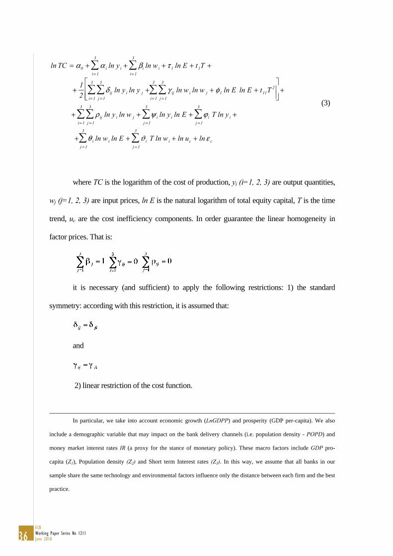
36ECBWorking Paper Series No 1211June 2010
ln TC = α0 + α i ln y ii= 1
3
∑ + βi ln wi + τ 1i= 1
3
∑ ln E + t1T +
+12
δ ij ln y i ln y jj = 1
3
∑ +i= 1
3
∑ γ ij ln wi ln w j + φ1 ln E ln Ej = 1
3
∑ + t11T2
i= 1
3
∑⎡
⎣ ⎢ ⎢
⎤
⎦ ⎥ ⎥
+
+ ρ ij ln y i ln w jj = 1
3
∑ + ψ i ln y i ln Ej = 1
3
∑ + ϕ i T ln y ij = 1
3
∑ +i= 1
3
∑
+ θ i ln wi ln Ej = 1
3
∑ + ϑ i T ln wij = 1
3
∑ + ln uc + ln ε c
(3)
where TC is the logarithm of the cost of production, yi (i=1, 2, 3) are output quantities,
wj (j=1, 2, 3) are input prices, ln E is the natural logarithm of total equity capital, T is the time
trend, uc are the cost inefficiency components. In order guarantee the linear homogeneity in
factor prices. That is:
it is necessary (and sufficient) to apply the following restrictions: 1) the standard
symmetry: according with this restriction, it is assumed that:
and
2) linear restriction of the cost function.
In particular, we take into account economic growth (LnGDPP) and prosperity (GDP per-capita). We also
include a demographic variable that may impact on the bank delivery channels (i.e. population density - POPD) and
money market interest rates IR (a proxy for the stance of monetary policy). These macro factors include GDP pro-
capita (Z1), Population density (Z2) and Short term Interest rates (Z3). In this way, we assume that all banks in our
sample share the same technology and environmental factors influence only the distance between each firm and the best
practice.

37ECB
Working Paper Series No 1211June 2010
Bank inputs and outputs are defined according to the value-added approach,
originally proposed by Berger and Humphrey (1992). We posit that labour, physical
capital and financial capital are inputs28, whereas demand deposits (y1), total loans (y2)
and other earning assets (y3) are outputs29. We also estimate the alternative revenue
efficiency measures: in this “alternative” approach, banks take input and output quantities
as given and we selected these measures since prices are often inaccurately measured in
banking.30 The revenue efficiency is estimated using the same translog functional model
adopted for the cost efficiency, by using as dependent variable the total bank’s revenue in
the revenue function. The bank input and output definition adopted is the same adopted to
estimate the cost efficiency.
28 Input prices are obtained as total personnel expenses over total assets (w1) , total depreciation and other capital
expenses over total fixed assets (w2) and total interest rate expenses over total funds (w3).
29 This selection of inputs and outputs follows the studies by Sathye (2001) and Dietsch and Lozano (2000), Aly et al.
(1990) and Hancock (1986), wherein the author develops a methodology based on user costs to determine the outputs
and inputs of a banking firm. Although off-balance sheet (OBS) items may play a role in generating bank value-added, we omit
to consider OBS items since our sample also includes small banks that do not have OBS items or data are not available in the
Bankscope database. By including the OBS in the output selection, the sample size would have been substantially reduced,
especially because we use a AR(3) process in model (1).
30 Berger and Mester (1997, p. 904) notes that “if prices are inaccurately measured –as is likely, given the available
banking data – the predicted part of the standard profit function would explain less of the variance of profits and yield
more error in the estimation of the efficiency terms ln u. In this event, it may be appropriate to try specifying other
variables in the profit function that might yield a better fit, such as the output quantity vector, y, as in the alternative
profit function”.

Work ing PaPer Ser i e Sno 1118 / november 2009
DiScretionary FiScal PolicieS over the cycle
neW eviDence baSeD on the eScb DiSaggregateD aPProach
by Luca Agnello and Jacopo Cimadomo