effects of water-supply reservoirs on streamflow in ... · effects of water-supply reservoirs on...

Prepared in cooperation with the Massachusetts Department of Environmental Protection

Effects of Water-Supply Reservoirs on Streamflow in Massachusetts

Scientific Investigations Report 2016–5123

U.S. Department of the InteriorU.S. Geological Survey

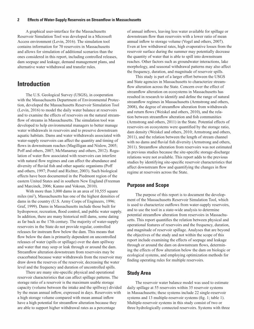
Cover. Photographs showing the Winchell Dam in Westfield, Massachusetts, during high flow conditions (left) on April 26, 2016 and low flow conditions (right) on July 27, 2012; photographs courtesy of Todd Richards, Massachusetts Division of Fisheries and Wildlife, used with permission.


By Sara B. Levin

Prepared in cooperation with the Massachusetts Department of Environmental Protection


U.S. Department of the InteriorU.S. Geological Survey

U.S. Department of the InteriorSALLY JEWELL, Secretary

U.S. Geological SurveySuzette M. Kimball, Director

U.S. Geological Survey, Reston, Virginia: 2016

For more information on the USGS—the Federal source for science about the Earth, its natural and living resources, natural hazards, and the environment—visit http://www.usgs.gov or call 1–888–ASK–USGS.

For an overview of USGS information products, including maps, imagery, and publications, visit http://store.usgs.gov.

Any use of trade, firm, or product names is for descriptive purposes only and does not imply endorsement by the U.S. Government.

Although this information product, for the most part, is in the public domain, it also may contain copyrighted materials as noted in the text. Permission to reproduce copyrighted items must be secured from the copyright owner.

Suggested citation:Levin, S.B., 2016, Effects of water-supply reservoirs on streamflow in Massachusetts: U.S. Geological Survey Scientific Investigations Report 2016–5123, 35 p., http://dx.doi.org/10.3133/sir20165123.

ISSN 2328-0328 (online)

http://www.usgs.gov

http://dx.doi.org/10.3133/sir20165123

iii

Acknowledgments

The author gratefully acknowledges the contributions of Richard Friend and Julie Butler of the Massachusetts Department of Environmental Protection, Linda Hutchins of the Massachusetts Department of Conservation and Recreation, and Laila Parker and Michelle Craddock of the Massachusetts Fish and Game’s Division of Ecological Restoration for their review comments for this report. Additionally, the author thanks Stacey Archfield, Gregory Granato, and Gardner Bent of the U.S. Geological Survey for their technical reviews of this report and Anna Glover of the U.S. Geological Survey for the editorial review of the report.

v

Contents

Acknowledgments ........................................................................................................................................iiiAbstract ...........................................................................................................................................................1Introduction.....................................................................................................................................................2

Purpose and Scope ..............................................................................................................................2Study Area..............................................................................................................................................2

Reservoir Simulation Tool .............................................................................................................................7Spillage Metrics .............................................................................................................................................8Sensitivity of Spillage to Reservoir Characteristics ...............................................................................11

Water Withdrawals ............................................................................................................................11Reservoir Size and Shape .................................................................................................................12Variability of Inflows ...........................................................................................................................15Groundwater Parameters ..................................................................................................................17

Application of the Reservoir Model for Selected Systems ...................................................................19Single-Reservoir Systems .................................................................................................................19Multiple-Reservoir Systems ..............................................................................................................20

Estimating Streamflow Alteration at Previously Unstudied Reservoirs .............................................24Monte Carlo Simulation .....................................................................................................................24Regression Equations for Spillage Metrics ....................................................................................27

Limitations .....................................................................................................................................................31Summary........................................................................................................................................................32References Cited..........................................................................................................................................33

Figures

1. Map showing drainage areas of 55 water-supply reservoirs in Massachusetts ..............3 2. Graph showing annual flow duration curves for estimated unaltered streamflow

at the Westfield (Montgomery) Reservoir in Montgomery, Massachusetts, for water years 1961 to 2004 .........................................................................................................................9

3. A, Graphs showing median annual flow duration curve and 95-percent confidence interval for estimated unaltered streamflow if no dam were present and reservoir spillage outflows at the Westfield (Montgomery) Reservoir. Boxplots representing the distribution of individual exceedance probability flows for each of the 44 water years at the B, 20th and C, 90th exceedance probabilities ..................................................10

4. Graphs showing A, monthly usage factors for 35 water-supply reservoir systems in Massachusetts and B, hypothetical monthly usage factor patterns use in reservoir sensitivity analyses ....................................................................................................................12

5. Boxplots showing change in A, median no-spill count, B, median no-spill duration, and C, annual flow duration deviation point resulting from monthly usage factor patterns with seasonal peaks compared to the mean usage pattern at 38 water- supply reservoirs in Massachusetts simulated at a withdrawal rate equal to 10 percent of the annual reservoir inflows .............................................................................13

6. Graph showing relation between usable storage and surface area for 55 water- supply reservoirs in Massachusetts .......................................................................................14

vi

7. Graphs showing A, the relative surface area to storage area relation for the Upper (Leahy) Reservoir in Lee, Massachusetts, and B, transformed into units of square miles and millions of gallons by multiplying the axes by the maximum storage volume and maximum surface area ..........................................................................15

8. Graphs showing the effect of the surface area to drainage area ratio on reservoir spillage as determined for the Upper (Leahy) Reservoir in Lee, Massachusetts, in a series of simulations where storage volume was kept fixed while increasing the maximum reservoir surface area ......................................................................................16

9. Graphs showing relation between reservoir inflow coefficient of variation and A–B, median no-spill count, C–D, median no-spill duration, and E–F, annual flow duration curve deviation point ..................................................................................................18

10. Graph showing effect of groundwater interactions on reservoir drawdown periods at the Granville Reservoir in Westfield, Massachusetts, from June 1962 through June 1969, simulated using an annual average withdrawal rate of 2.47 million gallons per day ............................................................................................................................19

11. Boxplots showing distributions of A, storage ratio, B, withdrawal ratio, C, average lateral distance from reservoir shoreline to the aquifer boundary, and D, transmissivity for selected reservoirs in Massachusetts and those used in Monte Carlo simulations ............................................................................................................25

12. Graph showing relation between the maximum surface area to drainage area ratio and the storage ratio for 55 water-supply reservoirs in Massachusetts .................26

13. Graphs showing regression and water balance model estimates for A, median no-spill count, B, median no-spill duration, and C, annual flow duration curve deviation point for 22 single-reservoir water-supply systems in Massachusetts and 4,000 Monte Carlo simulations ..........................................................................................29

14. Graphs showing relation of the A, median no-spill count, B, median no-spill duration, and C, annual flow duration curve deviation point with the withdrawal ratio across a range of surface to drainage area ratios typical for Massachusetts water-supply reservoirs .............................................................................................................30

15. Graph showing withdrawal ratio and reservoir surface area to drainage area ratio for Monte Carlo reservoir simulations for reservoirs in Massachusetts .................31

Tables

1. Reservoir characteristics for 35 reservoir systems in Massachusetts ...............................4 2. Median no-spill count and duration and annual flow duration curve deviation

point for 10 reservoirs in Massachusetts that intersect sand and gravel deposits ........20 3. Median no-spill count and duration and annual flow duration curve deviation

point for 22 single-reservoir systems in Massachusetts .....................................................21 4. Median no-spill count and duration and annual flow duration curve deviation

points for 13 multiple-reservoir systems in Massachusetts ................................................22 5. Fitted distribution parameters and goodness of fit tests for storage ratio,

withdrawal ratio, transmissivity, and lateral distance to the aquifer boundary for Massachusetts water supply reservoirs ..........................................................................26

6. Regression equation coefficients and summary statistics for regression equations relating median no-spill count and duration and annual flow duration curve deviation point for reservoirs in Massachusetts .......................................................28

vii

Conversion Factors

U.S. customary units to International System of Units

Multiply By To obtain

square mile (mi2) 2.590 square kilometer (km2) million gallons (Mgal) 3,785 cubic meter (m3)cubic foot per second (ft3/s) 0.02832 cubic meter per second (m3/s)

Datum

Vertical coordinate information is referenced to the North American Vertical Datum of 1988 (NAVD 88).

Horizontal coordinate information is referenced to the North American Datum of 1983 (NAD 83).

Elevation, as used in this report, refers to distance above the vertical datum.

Abbreviations

AFDC annual flow duration curve

MA SYE Massachusetts Sustainable-Yield Estimator

MUF monthly usage factor

SADA surface area to drainage area

USGS U.S. Geological Survey


By Sara B. Levin

AbstractState and local water-resource managers need modeling

tools to help them manage and protect water-supply resources for both human consumption and ecological needs. The U.S. Geological Survey, in cooperation with the Massachusetts Department of Environmental Protection, has developed a decision-support tool to estimate the effects of reservoirs on natural streamflow. The Massachusetts Reservoir Simulation Tool is a model that simulates the daily water balance of a reservoir. The reservoir simulation tool provides estimates of daily outflows from reservoirs and compares the frequency, duration, and magnitude of the volume of outflows from reservoirs with estimates of the unaltered streamflow that would occur if no dam were present. This tool will help environmental managers understand the complex interactions and tradeoffs between water withdrawals, reservoir operational practices, and reservoir outflows needed for aquatic habitats.

A sensitivity analysis of the daily water balance equation was performed to identify physical and operational features of reservoirs that could have the greatest effect on reservoir out-flows. For the purpose of this report, uncontrolled releases of water (spills or spillage) over the reservoir spillway were con-sidered to be a proxy for reservoir outflows directly below the dam. The ratio of average withdrawals to the average inflows had the largest effect on spillage patterns, with the highest withdrawals leading to the lowest spillage. The size of the sur-face area relative to the drainage area of the reservoir also had an effect on spillage; reservoirs with large surface areas have high evaporation rates during the summer, which can contrib-ute to frequent and long periods without spillage, even in the absence of water withdrawals. Other reservoir characteristics, such as variability of inflows, groundwater interactions, and seasonal demand patterns, had low to moderate effects on the frequency, duration, and magnitude of spillage.

The reservoir simulation tool was used to simulate 35 single- and multiple-reservoir systems in Massachusetts over a 44-year period (water years 1961 to 2004) under two water-use scenarios. The no-pumping scenario assumes no water withdrawal pumping, and the pumping scenario incorporates average annual pumping rates from 2000 to 2004. By comparing the results of the two scenarios, the

total streamflow alteration can be parsed into the portion of streamflow alteration caused by the presence of a reservoir and the additional streamflow alteration caused by the level of water use of the system.

For each reservoir system, the following metrics were computed to characterize the frequency, duration, and mag-nitude of reservoir outflow volumes compared with unaltered streamflow conditions: (1) the median number of days per year in which the reservoir did not spill, (2) the median duration of the longest consecutive period of no-spill days per year, and (3) the lowest annual flow duration exceedance probability at which the outflows are significantly different from estimated unaltered streamflow at the 95-percent confidence level. Most reservoirs in the study do not spill during the summer months even under no-pumping conditions. The median number of days during which there was no spillage was less than 365 for all reservoirs in the study, indicating that, even under reported pumping conditions, the reservoirs refill to full volume and spill at least once during nondrought years, typically in the spring.

Thirteen multiple-reservoir systems consisting of two or three hydrologically connected reservoirs were included in the study. Because operating rules used to manage multiple-reservoir systems are not available, these systems were simulated under two pumping scenarios, one in which water transfers between reservoirs are minimal and one in which reservoirs continually transferred water to intermediate or terminal reservoirs. These two scenarios provided upper and lower estimates of spillage under average pumping conditions from 2000 to 2004.

For sites with insufficient data to simulate daily water balances, a proxy method to estimate the three spillage metrics was developed. A series of 4,000 Monte Carlo simulations of the reservoir water balance were run. In each simulation, streamflow, physical reservoir characteristics, and daily climate inputs were randomly varied. Tobit regression equations that quantify the relation between streamflow alteration and physical and operational characteristics of reservoirs were developed from the results of the Monte Carlo simulations and can be used to estimate each of the three spillage metrics using only the withdrawal ratio and the ratio of the surface area to the drainage area, which are available statewide for all reservoirs.

2 Effects of Water-Supply Reservoirs on Streamflow in Massachusetts

A graphical user-interface for the Massachusetts Reservoir Simulation Tool was developed in a Microsoft Access environment (Levin, 2016). The simulation tool contains information for 70 reservoirs in Massachusetts and allows for simulation of additional scenarios than the ones considered in this report, including controlled releases, dam seepage and leakage, demand management plans, and alternative water withdrawal and transfer rules.

IntroductionThe U.S. Geological Survey (USGS), in cooperation

with the Massachusetts Department of Environmental Protec-tion, developed the Massachusetts Reservoir Simulation Tool (Levin, 2016) to model the daily water balance at reservoirs and to examine the effects of reservoirs on the natural stream-flow of streams in Massachusetts. The simulation tool was developed to help environmental managers to better manage water withdrawals in reservoirs and to preserve downstream aquatic habitats. Dams and water withdrawals associated with water-supply reservoirs can affect the quantity and timing of flows in downstream reaches (Magilligan and Nislow, 2005; Poff and others, 2007; McManamay and others, 2012). Regu-lation of water flow associated with reservoirs can interfere with natural flow regimes and can affect the abundance and diversity of fluvial fish and other aquatic organisms (Poff and others, 1997; Postel and Richter, 2003). Such biological effects have been documented in the Piedmont region of the eastern United States and in southern New England (Freeman and Marcinek, 2006; Kanno and Vokoun, 2010).

With more than 3,000 dams in an area of 10,555 square miles (mi2), Massachusetts has one of the highest densities of dams in the country (U.S. Army Corps of Engineers, 1996; Graf, 1999). Dams in Massachusetts include those built for hydropower, recreation, flood control, and public water supply. In addition, there are many historical mill dams, some dating as far back as the 17th century. The majority of water-supply reservoirs in the State do not provide regular, controlled releases for instream flow below the dam. This means that flow below the dam is primarily dependent on uncontrolled releases of water (spills or spillage) over the dam spillway and water that may seep or leak through or around the dam. Streamflow alteration downstream from reservoirs may be exacerbated because water withdrawals from the reservoir may draw down the reserves of the reservoir, decreasing the water level and the frequency and duration of uncontrolled spills.

There are many site-specific physical and operational reservoir characteristics that can affect spillage patterns. The storage ratio of a reservoir is the maximum usable storage capacity (volume between the intake and the spillway) divided by the mean annual inflow, expressed in days. Reservoirs with a high storage volume compared with mean annual inflow have a high potential for streamflow alteration because they are able to support higher withdrawal rates as a percentage

of annual inflows, leaving less water available for spillage or downstream flow than reservoirs with a lower ratio of mean annual inflow to storage volume (Vogel and others, 2007). Even at low withdrawal rates, high evaporative losses from the reservoir surface during the summer may potentially decrease the quantity of water that is able to spill into downstream reaches. Other factors such as groundwater interactions, lake morphology, and seasonal withdrawal patterns may also affect the frequency, duration, and magnitude of reservoir spills.

This study is part of a larger effort between the USGS and State agencies in Massachusetts to characterize stream-flow alteration across the State. Concern over the effect of streamflow alteration on ecosystems in Massachusetts has resulted in research to identify and define the range of natural streamflow regimes in Massachusetts (Armstrong and others, 2008), the degree of streamflow alteration from withdrawals and return flows (Weiskel and others, 2010), and the rela-tion between streamflow alteration and fish communities (Armstrong and others, 2011) in the State. Potential effects of reservoirs on ecosystems were quantified by the storage ratio, dam density (Weiskel and others, 2010; Armstrong and others, 2011), and the relation between the length of stream channel with no dams and fluvial fish diversity (Armstrong and others, 2011). Streamflow alteration from reservoirs was not estimated in previous studies because the site-specific storage-discharge relations were not available. This report adds to the previous studies by identifying site-specific reservoir characteristics that affect downstream flow and quantifying the changes in flow regime at reservoirs across the State.

Purpose and Scope

The purpose of this report is to document the develop-ment of the Massachusetts Reservoir Simulation Tool, which is used to characterize outflows from water-supply reservoirs, and to use the tool in a state-wide analysis to determine potential streamflow alteration from reservoirs in Massachu-setts. This report quantifies the relation between physical and operational features of reservoirs and the frequency, duration, and magnitude of reservoir spillage. Analyses that are beyond the objectives of the study and not within the scope of this report include examining the effects of seepage and leakage through or around the dam on downstream flows, determin-ing the effects of flow alteration below the dam on biologic or ecological systems, and employing optimization methods for finding operating rules for multiple reservoirs.

Study Area

The reservoir water balance model was used to estimate daily spillage at 55 reservoirs within 35 reservoir systems in Massachusetts; these systems include 22 single-reservoir systems and 13 multiple-reservoir systems (fig. 1; table 1). Multiple-reservoir systems in this study consist of two or three hydrologically connected reservoirs. Systems with three

Introduction 3

EXPL

AN

ATIO

N

Rese

rvoi

r dra

inag

e ar

eaTo

wn

boun

dary

Amhe

rst W

ater

Dep

artm

ent

1

. Atk

ins

Rese

rvoi

r

2. H

ill R

eser

voir

3

. Haw

ley

Rese

rvoi

r

4. A

met

hyst

Bro

ok In

take

Ashb

urnh

am/W

inch

endo

n Jo

int

Wat

er B

oard

5

. Upp

er N

auke

ag L

ake

Conc

ord

Wat

er D

epar

tmen

t

6. N

agog

Pon

dDa

nver

s W

ater

Dep

artm

ent

7

. Em

erso

n Br

ook

Rese

rvoi

r

8. M

iddl

eton

Pon

d

9. S

wan

Pon

dFa

ll Ri

ver W

ater

Dep

artm

ent

1

0. N

orth

Wat

uppa

Pon

d

11.

Cop

icut

Res

ervo

ir

Fitc

hbur

g W

ater

Dep

artm

ent

1

2. B

ickf

ord

Pond

1

3. M

are

Mea

dow

Res

ervo

ir

14.

Mee

tingh

ouse

Res

ervo

ir

15.

Wac

huse

tt La

ke

16.

Sco

tt Re

serv

oir

1

7. F

itchb

urg

Rese

rvoi

r

18.

Lov

ell R

eser

voir

Gree

nfie

ld W

ater

Dep

artm

ent

19.

Ley

den

Glen

Res

ervo

ir H

ingh

am/H

ull (

Aqua

rion

Wat

er C

ompa

ny)

2

0. A

ccor

d Po

ndHi

nsda

le W

ater

Dep

artm

ent

2

1. B

elm

ont R

eser

voir

Lee

Wat

er D

epar

tmen

t

22.

Sch

oolh

ouse

Res

ervo

ir

23.

Upp

er (L

eahy

) Res

ervo

ir

Leic

este

r Wat

er D

epar

tmen

t

24.

Hen

shaw

Pon

dLe

omin

ster

Dep

artm

ent o

f Pu

blic

Wor

ks

25.

Dis

tribu

ting

Rese

rvoi

r

26.

Mor

se R

eser

voir

2

7. H

ayne

s Re

serv

oir

2

8. S

imon

ds P

ond

2

9. G

oodf

ello

w P

ond

3

0. N

otow

n Re

serv

oir

3

1. F

all B

rook

Res

ervo

irLi

ncol

n W

ater

Dep

artm

ent

3

2. F

lints

Pon

d (S

andy

Pon

d)M

arlb

orou

gh D

epar

tmen

t of

Publ

ic W

orks

3

3. M

illha

m R

eser

voir

3

4. W

illia

ms

Lake

Milf

ord

Wat

er C

ompa

ny

35.

Ech

o La

ke

Wak

efie

ld W

ater

Dep

artm

ent

4

8. C

ryst

al L

ake

Wes

tbor

ough

Wat

er D

epar

tmen

t

49.

San

dra

Pond

Wes

tfiel

d W

ater

Dep

artm

ent

5

0. G

ranv

ille

Rese

rvoi

r

51.

Wes

tfiel

d Re

serv

oir,

in M

ontg

omer

y W

est S

prin

gfie

ld R

eser

voir

5

2. B

earh

ole

Rese

rvoi

rW

inch

este

r Wat

er D

epar

tmen

t

53.

Nor

th R

eser

voir

5

4. M

iddl

e Re

serv

oir

5

5. S

outh

Res

ervo

ir

Nor

th B

rook

field

Wat

er D

epar

tmen

t

36.

Doa

ne P

ond

3

7. H

orse

Pon

dPi

ttsfie

ld W

ater

Dep

artm

ent

3

8. A

shle

y La

ke

39.

Far

nham

Res

ervo

ir

40.

San

dwas

h Re

serv

oir

4

1. U

pper

Sac

kett

Rese

rvoi

r

42.

Cle

vela

nd B

rook

Res

ervo

irSc

ituat

e W

ater

Div

isio

n

43.

Sci

tuat

e Re

serv

oir

Sprin

gfie

ld W

ater

Dep

artm

ent

4

4. B

orde

n Br

ook

Rese

rvoi

r

45.

Cob

ble

Mou

ntai

n Re

serv

oir

Sout

h De

erfie

ld W

ater

Sup

ply

Dist

rict

4

6. R

oarin

g Br

ook

Rese

rvoi

r

47.

Wha

tely

Res

ervo

ir

13

45

42

10

2

44

11

7

52

50

19

3046

5

1

43

33

12

188

22

39

51

6

3549

2024

37

48

32

34

914

1516

17

21

23

27262528

29

31

34

36

384041

4753

54 55

70°

70°

71°

72°

73°

42°

42°3

0'

41°3

0'

41°

Base

map

from

U.S

. Geo

logi

cal S

urve

y an

d M

assa

chus

etts

Offi

ce o

f Ge

ogra

phic

Info

rmat

ion,

1:2

5,00

0-sc

ale

digi

tal d

ata

Stat

e Pl

ane

Coor

dina

te S

yste

mN

orth

Am

eric

an D

atum

of 1

983

040

KIL

OMET

ERS

040

MIL

ES20

20

Figu

re 1

. Dr

aina

ge a

reas

of 5

5 w

ater

-sup

ply

rese

rvoi

rs in

Mas

sach

uset

ts. R

eser

voirs

are

list

ed in

tabl

e 1.

4 Effects of Water-Supply Reservoirs on Streamflow in MassachusettsTa

ble

1.

Rese

rvoi

r cha

ract

eris

tics

for 3

5 re

serv

oir s

yste

ms

in M

assa

chus

etts

.

[With

draw

al ra

tio is

the

with

draw

al ra

te d

ivid

ed b

y th

e av

erag

e an

nual

inflo

w. S

tora

ge ra

tio is

the

usab

le st

orag

e di

vide

d by

the

aver

age

annu

al in

flow.

Ave

rage

with

draw

al a

nd w

ithdr

awal

ratio

are

tota

l by

syst

em a

nd d

o no

t inc

lude

val

ues f

or in

divi

dual

rese

rvoi

rs th

at a

re p

art o

f mul

tiple

-res

ervo

ir sy

stem

s. C

oeffi

cien

t of v

aria

tion

of st

ream

flow

is c

ompu

ted

only

for i

ndiv

idua

l res

ervo

irs a

nd d

oes n

ot a

pply

for

mul

tiple

-res

ervo

ir sy

stem

s. M

gal,

mill

ion

gallo

ns; M

gal/d

, mill

ion

gallo

ns p

er d

ay; m

i2 , sq

uare

mile

; DPW

, Dep

artm

ent o

f Pub

lic W

orks

]

Supp

lier

Rese

rvoi

r ID

(fi

g. 1

)Sy

stem

nam

e

Max

imum

us

able

st

orag

e

(Mga

l)

Mea

n an

-nu

al in

flow

(M

gal/d

)

Rese

rvoi

r su

rfac

e ar

ea

(mi2 )

Dra

inag

e ar

ea to

re

serv

oir

(mi2 )

Syst

em a

ver-

age

annu

al

with

draw

al,

2000

–200

4

(Mga

l/d)

Syst

em

with

draw

-al

ratio

Stor

age

ratio

(d

ays)

Surf

ace

area

to

drai

nage

ar

ea ra

tio

Coef

ficie

nt o

f va

riat

ion

of

stre

amflo

w

Am

hers

t Wat

er D

epar

tmen

t1

Atk

ins R

eser

voir

261.

667.

530.

076

a 12.

500.

830.

1134

.73

0.00

62.

57

Cen

tenn

ial s

yste

m30

.19

8.43

0.02

6.18

0.83

0.10

3.58

0.00

4

2H

ill R

eser

voir

20.7

45.

430.

010

4.05

3.82

0.00

32.

13

3H

awle

y R

eser

voir

6.59

2.12

0.01

01.

503.

110.

007

2.51

4A

met

hyst

Bro

ok in

take

re

serv

oir

2.86

0.88

0.00

20.

633.

240.

003

2.58

Ash

burn

ham

/Win

chen

don

5U

pper

Nau

keag

Lak

e1,

010.

141.

940.

483

1.37

1.06

0.55

521.

670.

351

3.17

Con

cord

Wat

er D

epar

tmen

t6

Nag

og P

ond

996.

860.

970.

442

0.77

0.09

0.09

1,02

5.63

0.57

33.

20

Dan

vers

Wat

er D

epar

tmen

tM

iddl

eton

Pon

d sy

stem

1,23

1.61

6.49

0.49

5.76

3.09

0.48

189.

790.

085

9Sw

an P

ond

189.

111.

360.

073

1.19

139.

160.

062

3.47

7Em

erso

n B

rook

Res

ervo

ir33

7.59

3.62

0.20

43.

2693

.27

0.06

33.

06

8M

iddl

eton

Pon

d70

4.91

1.51

0.21

51.

3246

6.56

0.16

43.

11

Fall

Riv

er W

ater

Dep

artm

ent

Nor

th W

atup

pa sy

stem

10,3

37.9

718

.32

3.80

14.0

712

.89

0.70

564.

410.

270

11C

opic

ut R

eser

voir

3,79

8.16

7.53

0.96

95.

6650

4.46

0.17

12.

09

10N

orth

Wat

uppa

Pon

d6,

539.

8110

.79

2.83

48.

4160

6.25

0.33

71.

88

Fitc

hbur

g W

ater

Dep

artm

ent

Love

ll R

eser

voir

syst

em1,

229.

498.

080.

355.

830.

180.

0215

2.26

0.06

0

17Fi

tchb

urg

Res

ervo

ir68

3.80

2.68

0.23

81.

9025

5.11

0.12

63.

17

16Sc

ott R

eser

voir

185.

551.

080.

056

0.73

171.

510.

076

3.62

18Lo

vell

Res

ervo

ir36

0.14

4.31

0.05

83.

2083

.50

0.01

83.

29

Mee

tingh

ouse

syst

em3,

300.

319.

590.

966.

992.

710.

2834

4.31

0.13

7

12B

ickf

ord

Pond

903.

524.

230.

260

3.02

213.

620.

086

2.75

13M

are

Mea

dow

Res

ervo

ir1,

751.

193.

530.

454

2.64

495.

630.

172

3.27

14M

eetin

ghou

se R

eser

voir

645.

601.

820.

246

1.32

354.

260.

186

3.11

15W

achu

sett

Lake

389.

771.

950.

194

1.32

0.35

0.18

199.

490.

147

2.28

Gre

enfie

ld W

ater

Dep

artm

ent

19Le

yden

Gle

n R

eser

voir

43.1

06.

870.

010

5.15

0.57

0.08

6.27

0.00

22.

82

Hin

gham

/Hul

l (A

quar

ion

Wat

er C

ompa

ny)

20A

ccor

d Po

nd21

8.78

0.99

0.16

40.

790.

590.

5922

0.35

0.20

92.

48

Hin

sdal

e W

ater

Dep

artm

ent

21B

elm

ont R

eser

voir

36.1

50.

580.

018

0.37

0.15

0.26

62.5

60.

048

2.88

Lee

Wat

er D

epar

tmen

t22

Scho

olho

use

Res

ervo

ir12

7.77

4.34

0.06

12.

940.

510.

1229

.46

0.02

12.

32

23U

pper

(Lea

hy) R

eser

voir

348.

280.

980.

072

0.63

0.54

0.55

355.

430.

114

2.76

Introduction 5Ta

ble

1.

Rese

rvoi

r cha

ract

eris

tics

for 3

5 re

serv

oir s

yste

ms

in M

assa

chus

etts

.—Co

ntin

ued

[With

draw

al ra

tio is

the

with

draw

al ra

te d

ivid

ed b

y th

e av

erag

e an

nual

inflo

w. S

tora

ge ra

tio is

the

usab

le st

orag

e di

vide

d by

the

aver

age

annu

al in

flow.

Ave

rage

with

draw

al a

nd w

ithdr

awal

ratio

are

tota

l by

syst

em a

nd d

o no

t inc

lude

val

ues f

or in

divi

dual

rese

rvoi

rs th

at a

re p

art o

f mul

tiple

-res

ervo

ir sy

stem

s. C

oeffi

cien

t of v

aria

tion

of st

ream

flow

is c

ompu

ted

only

for i

ndiv

idua

l res

ervo

irs a

nd d

oes n

ot a

pply

for

mul

tiple

-res

ervo

ir sy

stem

s. M

gal,

mill

ion

gallo

ns; M

gal/d

, mill

ion

gallo

ns p

er d

ay; m

i2 , sq

uare

mile

; DPW

, Dep

artm

ent o

f Pub

lic W

orks

]

Supp

lier

Rese

rvoi

r ID

(fi

g. 1

)Sy

stem

nam

e

Max

imum

us

able

st

orag

e

(Mga

l)

Mea

n an

-nu

al in

flow

(M

gal/d

)

Rese

rvoi

r su

rfac

e ar

ea

(mi2 )

Dra

inag

e ar

ea to

re

serv

oir

(mi2 )

Syst

em a

ver-

age

annu

al

with

draw

al,

2000

–200

4

(Mga

l/d)

Syst

em

with

draw

-al

ratio

Stor

age

ratio

(d

ays)

Surf

ace

area

to

drai

nage

ar

ea ra

tio

Coef

ficie

nt o

f va

riat

ion

of

stre

amflo

w

Leic

este

r (C

herr

y Va

lley

and

Roc

hdal

e W

ater

Dis

trict

)24

Hen

shaw

Pon

d92

.80

1.20

0.05

70.

880.

260.

2277

.38

0.06

52.

89

Leom

inst

er D

PW–W

ater

Div

isio

n31

Fall

Bro

ok R

eser

voir

352.

921.

710.

141

1.21

0.88

0.52

206.

920.

117

3.54

Sim

onds

Pon

d sy

stem

735.

336.

190.

404.

552.

320.

3711

8.75

0.08

8

30N

otow

n R

eser

voir

709.

315.

300.

384

3.96

133.

750.

097

2.58

29G

oodf

ello

w P

ond

9.18

0.61

0.00

70.

4114

.96

0.01

62.

84

28Si

mon

ds P

ond

16.8

40.

280.

010

0.18

61.1

90.

055

4.36

Dis

tribu

ting

Res

ervo

ir sy

stem

182.

452.

600.

120.

850.

870.

3370

.21

0.14

3

27H

ayne

s Res

ervo

ir12

9.83

0.52

0.09

40.

3425

0.83

0.27

53.

68

26M

orse

Res

ervo

ir45

.50

0.43

0.02

10.

2810

5.47

0.07

63.

38

25D

istri

butin

g R

eser

voir

7.12

1.65

0.00

71.

144.

320.

006

2.82

Linc

oln

Wat

er D

epar

tmen

t32

Flin

ts P

ond

505.

600.

710.

253

0.55

0.38

0.53

708.

270.

462

3.40

Mar

lbor

ough

DPW

Mill

ham

syst

em31

3.02

4.67

0.21

3.65

1.40

0.30

67.1

00.

057

33W

illia

ms L

ake

0.00

0.35

0.09

90.

260.

000.

389

4.12

34M

illha

m R

eser

voir

313.

024.

310.

108

3.40

72.5

70.

032

2.46

Milf

ord

Wat

er C

ompa

ny35

Echo

Lak

e46

1.64

1.61

0.16

51.

261.

400.

8728

7.17

0.13

13.

40

Nor

th B

rook

field

Wat

er D

epar

tmen

tD

oane

Pon

d sy

stem

291.

312.

140.

141.

540.

420.

2013

6.19

0.09

0

37H

orse

Pon

d24

8.70

1.10

0.10

00.

7922

5.66

0.12

63.

10

36D

oane

Pon

d42

.61

1.04

0.03

90.

7541

.09

0.05

23.

15

Pitts

field

Wat

er D

epar

tmen

t38

Ash

ley

Lake

481.

233.

580.

179

2.43

0.21

0.06

134.

540.

074

2.37

42C

leve

land

Bro

ok R

eser

voir

1,82

5.09

19.2

50.

244

b 13.

747.

960.

4194

.79

0.01

81.

90

Farn

ham

Res

ervo

ir sy

stem

738.

116.

780.

172.

152.

230.

3310

8.87

0.07

9

40Sa

ndw

ash

Res

ervo

ir26

0.86

2.53

0.10

41.

6710

3.28

0.06

22.

44

39Fa

rnha

m R

eser

voir

477.

254.

250.

065

0.48

112.

190.

137

2.31

41U

pper

Sac

kett

Res

ervo

ir16

2.73

1.27

0.03

40.

860.

080.

0612

7.72

0.03

92.

70

Scitu

ate

Wat

er D

ivis

ion

43Sc

ituat

e R

eser

voir

145.

004.

350.

091

3.50

0.63

0.14

33.3

70.

026

2.52

Sout

h D

eerfi

eld

Wat

er S

uppl

y D

istri

ctW

hate

ly R

eser

voir

syst

em18

3.89

6.81

0.04

5.19

0.68

0.10

27.0

00.

007

46R

oarin

g B

rook

Res

ervo

ir17

3.74

5.21

0.03

23.

9733

.36

0.00

82.

55

47W

hate

ly R

eser

voir

10.1

51.

600.

003

1.22

6.33

0.00

23.

28


ble

1.

Rese

rvoi

r cha

ract

eris

tics

for 3

5 re

serv

oir s

yste

ms

in M

assa

chus

etts

.—Co

ntin

ued

[With

draw

al ra

tio is

the

with

draw

al ra

te d

ivid

ed b

y th

e av

erag

e an

nual

inflo

w. S

tora

ge ra

tio is

the

usab

le st

orag

e di

vide

d by

the

aver

age

annu

al in

flow.

Ave

rage

with

draw

al a

nd w

ithdr

awal

ratio

are

tota

l by

syst

em a

nd d

o no

t inc

lude

val

ues f

or in

divi

dual

rese

rvoi

rs th

at a

re p

art o

f mul

tiple

-res

ervo

ir sy

stem

s. C

oeffi

cien

t of v

aria

tion

of st

ream

flow

is c

ompu

ted

only

for i

ndiv

idua

l res

ervo

irs a

nd d

oes n

ot a

pply

for

mul

tiple

-res

ervo

ir sy

stem

s. M

gal,

mill

ion

gallo

ns; M

gal/d

, mill

ion

gallo

ns p

er d

ay; m

i2 , sq

uare

mile

; DPW

, Dep

artm

ent o

f Pub

lic W

orks

]

Supp

lier

Rese

rvoi

r ID

(fi

g. 1

)Sy

stem

nam

e

Max

imum

us

able

st

orag

e

(Mga

l)

Mea

n an

-nu

al in

flow

(M

gal/d

)

Rese

rvoi

r su

rfac

e ar

ea

(mi2 )

Dra

inag

e ar

ea to

re

serv

oir

(mi2 )

Syst

em a

ver-

age

annu

al

with

draw

al,

2000

–200

4

(Mga

l/d)

Syst

em

with

draw

-al

ratio

Stor

age

ratio

(d

ays)

Surf

ace

area

to

drai

nage

ar

ea ra

tio

Coef

ficie

nt o

f va

riat

ion

of

stre

amflo

w

Sprin

gfiel

d W

ater

Dep

artm

ent

Cob

ble

Mou

ntai

n sy

stem

23,0

94.0

056

.49

2.00

43.5

236

.57

0.65

408.

790.

046

44B

orde

n B

rook

Res

ervo

ir2,

524.

909.

940.

339

7.64

254.

060.

044

2.18

45C

obbl

e M

ount

ain

Res

ervo

ir20

,569

.10

46.5

61.

659

35.8

844

1.82

0.04

61.

94

Wak

efiel

d W

ater

Dep

artm

ent

48C

ryst

al L

ake

169.

810.

940.

130

0.74

0.28

0.30

179.

940.

175

3.00

Wes

t Spr

ingfi

eld

Wat

er D

epar

tmen

t52

Bea

rhol

e R

eser

voir

92.5

26.

360.

027

5.51

0.73

0.11

14.5

40.

005

2.10

Wes

tbor

ough

Wat

er D

epar

tmen

t49

Sand

ra P

ond

163.

681.

510.

101

1.10

0.67

0.44

108.

580.

092

2.51

Wes

tfiel

d W

ater

Dep

artm

ent

50G

ranv

ille

Res

ervo

ir66

3.85

7.00

0.11

65.

142.

470.

3594

.88

0.02

32.

28

51W

estfi

eld

(Mon

tgom

ery)

R

eser

voir

208.

913.

180.

057

2.47

0.00

0.00

65.6

60.

023

2.31

Win

ches

ter W

ater

Dep

artm

ent

Sout

h R

eser

voir

syst

em77

9.64

1.43

0.30

1.10

1.10

0.77

545.

440.

273

53N

orth

Res

ervo

ir24

7.95

0.69

0.09

30.

5335

9.40

0.17

63.

27

54M

iddl

e R

eser

voir

120.

400.

290.

082

0.22

418.

140.

373

4.42

55So

uth

Res

ervo

ir41

1.29

0.45

0.12

40.

3591

0.87

0.35

84.

20a D

rain

age

area

incl

udes

add

ition

al d

rain

age

area

to D

ean

Bro

ok, w

hich

has

bee

n di

verte

d to

flow

into

Atk

ins R

eser

voir.

b Dra

inag

e ar

ea in

clud

es a

dditi

onal

dra

inag

e ar

ea to

Cad

y B

rook

and

Win

dsor

Bro

ok, w

hich

hav

e be

en d

iver

ted

to fl

ow in

to C

leve

land

Bro

ok R

eser

voir.

Reservoir Simulation Tool 7

reservoirs are configured either in linear series or in parallel with two upper reservoirs transferring water to the terminal reservoir. Reservoir characteristics—including daily inflow, precipitation, evaporation, relation between stage and storage, aquifer properties, and mean annual water withdrawals—were compiled in Waldron and Archfield (2006) and Levin and others (2011). All reservoirs in this study were simulated from October 1, 1960, to September 30, 2004, which coincides with the simulation period of the Massachusetts Sustainable-Yield Estimator (MA SYE) tool (Archfield and others, 2009), which was used to estimate daily reservoir inflows. Site-specific information regarding seepage and leakage of water through or around dams was not available for reservoirs included in the study. Due to this lack of information, leakage was assumed to be zero for all simulations.

Reservoir Simulation ToolThe Massachusetts Reservoir Simulation Tool simulates

single- or multiple-reservoir systems using an equation to calculate daily reservoir water balance. This approach has been used in previous studies to determine the maximum yield of selected drinking water reservoir systems in Massachusetts (Waldron and Archfield, 2006; Levin and others, 2011). For the purpose of this report, a reservoir system is defined as a single reservoir or a group of hydrologically connected reser-voirs from which water is withdrawn for public water supply. Note that a particular municipality may receive water from a combination of multiple-reservoir systems, groundwater wells, or purchased water from other systems.

The reservoir water balance, in million gallons per day, can be calculated as follows:

Si = Si–1 + AwiQsti – αiQwdi + CAri (Pi – Ei) – Qspi ±Qgwi -Qcri ±Qti – Li, (1)

where i is the daily simulation time step; Si is the volume of water in usable storage for

the current day, in million gallons; Awi is the reservoir drainage area, in square miles; Qsti is the daily reservoir inflow per unit drainage

area, in million gallons per day per square mile;

αi is a monthly usage factor, dimensionless; Qwdi are the average daily withdrawal, in million

gallons; C is a unit conversion factor equal to

1,101,117.14743 million gallons per cubic mile;

Ari is the area of the reservoir surface, in square miles;

Pi is the daily precipitation converted to length, in miles;

Ei is the daily evaporation from the reservoir surface converted to length, in miles;

Qspi is the uncontrolled spill, in million gallons; Qgwi are the groundwater contributions or losses

for the current day, in million gallons; Qcri are the controlled releases for instream flow,

in million gallons; Qti is the water transferred from the reservoir to

a receiving reservoir or into the reservoir from a contributing reservoir (multiple-reservoir systems only), in million gallons; and

Li is the leakage or seepage through or around the dam, in million gallons.

The equation for reservoir water balance (equation 1) is solved for every day of the period of record, starting with a full reservoir volume. Solving the reservoir water balance equation produces a time series of daily spillage volumes over the period of record. At each daily time step, the storage volume of the reservoir is estimated from the previous day’s storage, precipitation onto the reservoir’s surface, streamflow into the reservoir, evaporation off of the reservoir surface, withdrawals from the reservoir, groundwater contributions in or out of the system, seepage or leakage, controlled releases, and water transfers into or out of the reservoirs. If the daily storage (Si) exceeds the maximum capacity for the reservoir, uncontrolled spillage (Qspi) occurs and is equal to the differ-ence between these two values. When daily storage is less than the maximum capacity, spillage is zero. If the daily storage (Si) is insufficient to supply the specified withdrawal rate (Qwdi), then the volume of water that is available in storage (if any) is used for withdrawal and the simulation continues, resuming full withdrawal volumes when there is sufficient storage.

Reservoir volume and surface area data for different reservoir elevations are used to scale precipitation, evapora-tion, and inflow volumes from the lake surface. The daily surface area of the lake changes relative to the current reser-voir storage. At each time step, interpolation of the volume and surface area data is used to determine the reservoir surface area (Ari) based on the storage volume for the previous day. Precipitation (Pi) and, evaporation (Ei) are entered into the model in units of depth (in inches, which are then converted to miles) and multiplied by the surface area to compute the daily volume of precipitation and evaporation. The drainage area of the reservoir changes inversely to the daily surface area. That is, when the surface area decreases, the drainage area increases by the same amount. The drainage area for each day is used to scale the reservoir inflows in the same manner as precipitation and evaporation. Reservoir inflows (Qsti) in units of volume per square mile of drainage area and are multiplied by the daily drainage area to compute the daily inflow volume in million gallons. For the purposes of this study, controlled releases (Qcri) and seepage and leakage (Li) were assumed to be zero in all cases. The Massachusetts Reservoir Simulation Tool (Levin, 2016) has additional simulation options, allowing


for demand management scenarios that were not included in this study.

Gains and losses from groundwater are estimated using a set of equations based on an analytical solution to the groundwater flow equation for the case of one-dimensional flow in a finite-width aquifer bounded by a linear surface-water feature developed by Archfield and Carlson (2006). Groundwater interactions in the model are caused by current and past changes in reservoir stage. When the reservoir surface elevation decreases below the water table due a decrease in storage, water from the aquifer will flow into the reservoir until the reservoir stage and aquifer water table are in equilibrium. Conversely, when reservoir surface elevations rise above the water table elevation, water from the reservoir is lost to the surrounding aquifer. At each time step there may also be additional groundwater gains or losses from the time-lagged effects of previous changes in reservoir storage.

Many reservoir systems are comprised of multiple reservoirs that are hydrologically connected. Multiple-reservoir systems can be configured in many ways and can transfer water by gravity through a river or open channel to a downstream reservoir, or by pumping water from one reservoir to another through a pipeline. Drainage areas in a multiple-reservoir system may be nested or nonnested. In a nested system, the drainage area of the contributing reservoir lies within an upstream portion of the receiving reservoir drainage area. In nested systems, water transferred from the contributing reservoir to meet demand as well as any controlled or uncontrolled spills and dam seepage and leakage from the contributing reservoir are added to the inflows of the receiving reservoir. Drainage areas in nonnested systems are not connected by a stream or natural drainage pathway. In nonnested systems, only the volume of water that is pumped from the contributing reservoir is added to the inflows of the receiving reservoir. Controlled and uncontrolled spills and seepage or leakage from the contributing reservoir dam are lost from the system and contribute to downstream flow below the contributing reservoir. The volume and timing of water that is transferred to a receiving reservoir (Qti) either through pumping or by gravity is specified in monthly operating rules within the model for each reservoir in the system. Operating rules in the Massachusetts Reservoir Simulation Tool (Levin, 2016) may be specified such that water transfers only occur when the receiving reservoir storage volume fall below a threshold value.

Spillage MetricsFor the purposes of this study, uncontrolled reservoir

spills are used as a proxy for streamflow below the dam. The reservoirs included in this study do not regularly release water to augment flow downstream from the reservoir. Therefore, streamflow below the dam is primarily dependent upon uncontrolled spills over the dam spillway and water seepage

and leakage through or around the dam. Although seepage and leakage can contribute to downstream flow, it is beyond the scope of this study to examine the effects of these sources of water, which vary widely from one location to another, on the patterns of flow downstream from reservoirs.

Typically, reservoirs in Massachusetts stop spilling in the summer when withdrawals and evaporation are greater than inflows to the reservoir. Reservoirs refill partially or completely in the winter and spring when inflow is greater than evaporation and withdrawals. Three spillage metrics were developed to characterize the magnitude, frequency, and duration of reservoir spillage: (1) the median no-spill count, (2) the median no-spill duration, and (3) annual flow duration curve (AFDC) deviation point, described later in this section. The frequency of no-spill periods was characterized by the median no-spill count. This metric was computed by finding the median number of days per water year1 during which the uncontrolled spillage (Qspi) is equal to zero for each of the 44 water years of simulation and then computing the median of the 44 medians. The duration of no-spill periods was characterized by the median no-spill duration, which was computed by finding the longest period of consecutive no-spill days each water year of the simulation and computing the median of the 44 no-spill durations.

The magnitude of reservoir spillage was characterized by the annual flow duration curve (AFDC) deviation point, which is a metric that was derived from the AFDCs of both the reservoir spillage and the estimated unaltered flow (estimated streamflow that would occur if the dam were not present). The AFDC is the relation between daily streamflow quantiles and an exceedance probability for the period of 1 water year. The exceedance probability is the frequency that a particular flow is exceeded during the water year. For example, 20 percent of the daily flows during a water year are greater than the streamflow at the 20 percent exceedance probability. An AFDC can be computed for each water year of the simulation period. Figure 2 shows an example AFDC for the Westfield (Montgomery) Reservoir (fig. 1, reservoir 51) in Montgomery. For this study, all reservoirs were simulated for the 44-water year period of record from October 1, 1960, to September 30, 2004. The median AFDC is constructed from the median of the 44 flows at each exceedance probability. Confidence intervals can be constructed around the median AFDC (Vogel and Fennessey, 1994) to show the interannual streamflow variability at a particular exceedance probability (fig. 2).

The median AFDC and the 95-percent confidence interval around it represent the unique flow signature of a stream. The median AFDC represents median daily flow magnitudes throughout the year, whereas the confidence intervals represent flow magnitudes during dry and wet periods from the period of record. AFDCs with steep slopes result from runoff-dominated streams with more seasonal variability and are typical across most of Massachusetts. AFDCs with flat slopes result from

1A water year is the 12-month period from October 1 through September 30 of the following year and is designated by the calendar year in which it ends.

Spillage Metrics 9

0.001

0.01

0.1

1

10

100

1,000

Daily

stre

amflo

w, i

n cu

bic

feet

per

sec

ond

0 20 40 60 80 100

Exceedance probability, in percent

Median

95-percent confidence interval

EXPLANATION

Figure 2. Annual flow duration curves (AFDCs) for estimated unaltered streamflow at the Westfield (Montgomery) Reservoir in Montgomery, Massachusetts, for water years 1961 to 2004 (colored lines).

base flow-dominated streams with less seasonal variability. Whereas the slope of the median AFDC indicates the seasonal variability at a site, the width of the confidence interval around the median AFDC represents the interannual variability in streamflow for the period of record. Flows at both ends of the AFDC may vary by an order of magnitude or more from one year to the next. The monthly distribution of flows in an AFDC varies from one stream to another, but in general for streams in this study, low flows at more than the 80 percent exceedance probability represent summer flows from July through September, and high flows at less than the 20 percent exceedance probability represent spring and winter flows.

Streamflow alteration below the dam was assessed by computing the AFDC deviation point. This metric compares the median AFDC of the reservoir spillage with that of the estimated unaltered streamflow if no dam were present. Unaltered streamflow at the dam was computed using the MA SYE (Archfield and others, 2009). This is the same method used to compute inflows to the reservoir in the water balance equation (equation 1). The difference between the computed inflows and the unaltered streamflow is that the drainage area used to compute inflows includes only the drainage to the reservoir, whereas the drainage area for unaltered streamflow includes an additional area equal to the reservoir surface.

A comparison of the AFDCs from unaltered streamflow and spillage shows how reservoir spillage differs from natural conditions during wet, dry, and median hydrologic conditions. For example, figure 3A shows the median AFDC and confidence intervals for unaltered streamflow and

spillage volumes for the Westfield (Montgomery) Reservoir (fig. 1, reservoir 51). At exceedance probabilities less than 50 percent, there is little or no difference between the AFDC of the spillage volumes and that of the unaltered streamflow, indicating that these high streamflows, which occur mainly in spring and winter, are not altered by the presence of the reservoir even in dry or wet years. The median AFDC of the spillage volumes begins to deviate from that of the unaltered flows between an exceedance probability of 70 and 80 percent, indicating that, during median hydrologic conditions (neither exceedingly wet nor dry years), the lowest 20 or 30 percent of spillage volumes, which typically occur during summer, are lower than unaltered streamflow.

The AFDC deviation point statistically quantifies the comparison of the AFDCs of unaltered streamflow and reservoir spillage volumes. At each exceedance probability, there are 44 values, one for each year of the simulation, for both unaltered streamflow and spillage volumes. The two-sample Kolmogorov-Smirnov test (Conover, 1980) was used to determine if the distribution of the spillage volumes was significantly different than the distribution of the estimated unaltered streamflow at the 95-percent confidence level for each exceedance probability. The Kolmogorov-Smirnov test is a nonparametric test to determine if two sample datasets come from the same population. A p-value less than 0.05 indicates that the sample distributions differ in either median value, variability, or distribution shape at the 5 percent confidence level. For example, figures 3B and C shows the distribution of unaltered streamflow and spillage volumes at the 20-percent and 90-percent exceedance probabilities at the Westfield (Montgomery) Reservoir and correspond to the distribution of flows in the highlighted regions of the median AFDCs shown in figure 3A. The p-value of the Kolmogorov-Smirnov test for the 20-percent exceedance probability flows was 0.99, indicating that the spillage volumes do not differ significantly from the unaltered streamflow. At the 90-percent exceedance probability, the p-value is less than 0.001, indicating that the distribution of spillage flows is significantly different from unaltered streamflow.

The AFDC deviation point is the exceedance probability at which the distribution of spillage volumes begins to significantly differ from the distribution of unaltered flows at the 0.05 significance level, based on the Kolmogorov-Smirnov test. The AFDC deviation point is computed by performing the Kolmogorov-Smirnov test on unaltered and spillage flows for each exceedance probability, starting with the lowest flows (exceedance probability of 100 percent) and working toward the highest flows (exceedance probability of 0 percent). Typically, the lowest flows are the most highly altered, and alteration becomes gradually less statistically significant as the flows increase. The AFDC deviation point is the lowest exceedance probability at which the p-value of the Kolmogorov-Smirnov test is less than 0.05. For example, the AFDC deviation point for the Westfield (Montgomery) Reservoir is at the 79 percent exceedance probability (fig. 3A, red line). This means that the highest 79 percent of


0.001

0.01

0.1

1

10

100

1,000

0 20 40 60 80 100

2.0

1.5

1.0

0.5

0.0

0.25

0.75

1.25

1.75

2.2511

10

9

8

7

6

5

4

3

2Spillage flows Spillage flowsUnaltered flows Unaltered flows

Daily

stre

amflo

w, i

n cu

bic

feet

per

sec

ond

Daily

stre

amflo

w, i

n cu

bic

feet

per

sec

ond

Daily

stre

amflo

w, i

n cu

bic

feet

per

sec

ond

Exceedance probability, in percent

Estimated unaltered flows—Dashed lines indicate 95-percent confidence interval

Spillage at the dam—Dashed lines indicate 95-percent confidence interval

EXPLANATION

Outlier

75th percentile

90th percentile

10th percentile

50th percentile—Median

25th percentile

Exceedance probability

AFDC deviation

A

B C

Figure 3. A, Median annual flow duration curve (AFDC) and 95-percent confidence interval for estimated unaltered streamflow if no dam were present (black lines) and reservoir spillage outflows (blue lines) at the Westfield (Montgomery) Reservoir. Red line shows the AFDC deviation point which delineates the exceedance probability at which spillage flows become significantly different from unaltered streamflow. Boxplots representing the distribution of individual exceedance probability flows for each of the 44 water years at the B, 20th and C, 90th exceedance probabilities (highlighted in gray in part A).

Sensitivity of Spillage to Reservoir Characteristics 11

the flows from uncontrolled spillage during the year are not significantly different from unaltered conditions, whereas the lowest 21 percent of annual flows are significantly lower than unaltered streamflow. An AFDC deviation point of 1 indicates that there is no significant difference between unaltered flows and reservoir spillage patterns at any exceedance probability, and an AFDC deviation point of 0 indicates that flows at all exceedance probabilities have been significantly altered.

The inclusion of the AFDC deviation point in this report is intended to give an objective metric of overall potential alteration in streamflow below a reservoir for classification and screening purposes, so that environmental managers can determine which sites may be at the greatest risk of having their ecosystem affected from a change in streamflow regime. It is important to note that a statistically significant difference in flows at a certain exceedance probability is not a direct indicator of ecosystem or biological change. The estimation of ecosystem response to flow regulation is an active research area, and many other variables, such as the extent of impervious surface within the watershed and changes in stream temperature and geomorphology, can also affect biotic communities (Poff and others, 1997; Postel and Richter, 2003). Although studies have shown relations between changes in streamflow regimes and aquatic communities (Poff and Zimmerman, 2010; Armstrong and others, 2011), it is beyond the scope of this study to determine at what point a change in the AFDC of a regulated stream affects biologic or ecological systems.

Sensitivity of Spillage to Reservoir Characteristics

Spillage from a reservoir occurs when a reservoir is at full capacity and daily water inputs from streamflow, pre-cipitation, and groundwater flowing into the reservoir exceed losses from withdrawals, evaporation, and water flowing into the aquifer. There are many factors that can potentially affect reservoir spillage patterns, including the withdrawal rate, the natural variability of inflows and climate, the size of the reservoir, the magnitude of groundwater interactions with the reservoir, and seepage and leakage through or around the dam (assumed to be zero in this study). A sensitivity analysis of the reservoir water balance model was performed to examine the effects of different reservoir characteristics on spillage patterns by changing one component of the water balance equation while holding all other terms constant. For the purposes of this report, a reservoir failure is defined as any period equal to one day or more during which there is insufficient water available in the reservoir to supply the specified withdrawal rate. All analyses in this report assumed a no-fail withdrawal condi-tions (that is, withdrawal rates were set such that there were no reservoir failures during the simulation period). This analysis was performed in order to gain a better understanding of the interactions between reservoir characteristics and spillage. A

conceptual understanding of reservoir and spillage interactions may help environmental managers identify reservoirs most at risk of flow alteration and interpret model results.

Water Withdrawals

Water withdrawals reduce the amount of water that is available for spillage. During average meteorological condi-tions, streamflow into the reservoir and water withdrawals from the reservoir are generally much larger in magnitude than precipitation or evaporation from the reservoir surface and are the primary mechanisms that control drawdown and refill of water-supply reservoirs. Withdrawal rates that are large compared with inflows will result in less frequent spillage than withdrawal rates that are small compared with inflows. The withdrawal ratio is defined as the mean annual withdrawal from a reservoir divided by the mean annual streamflow into the reservoir. The withdrawal ratio is a useful metric for comparing the effects of water withdrawals on spillage across systems of different sizes. Reported withdrawal ratios for 2000 to 2004 range from 0 to 0.87, with a median of 0.30 for the 35 reservoir systems in this study (table 1).

Demand for water supplies varies throughout the year, typically rising slightly during summer months due to outdoor water use. Monthly usage factors (MUFs) are applied in the water balance equation (αi in equation 1) to convert the annual average withdrawal into monthly volumes. For a given year, the MUF for a reservoir system are calculated by dividing the monthly reported withdrawal volume by the average annual withdrawal volume. Average MUFs were compiled for each of the 35 reservoir systems in Levin and others (2011) from reported withdrawals from 2000 to 2004 (fig. 4A). The average MUF curve for these systems is relatively steady for most of the year, with a slight increase from June until August; however, there is considerable variability in MUF patterns from one reservoir system to another. In systems where the total demand for water for a particular water supplier is met by several different reservoirs or a combination of reservoirs, groundwater wells, or water purchased from another supplier, the MUF pattern for a reservoir may not resemble the typical water demand pattern. For example, the Town of Concord typically only uses Nagog Pond (fig. 1, reservoir 6) during the summer months to augment groundwater wells that supply drinking water throughout the rest of the year. Because of the limited use of this reservoir, the MUF values during the summer months are much higher than other reservoirs that operate year-round and decrease to zero for the months of October through April (fig. 4A).

To examine the effect of different seasonal withdrawal patterns on reservoir spillage, reservoirs were simulated under four MUF curves that represent average pumping conditions as well as hypothetical seasonal withdrawal patterns that have maximum usage in spring, summer, and fall (fig. 4B). Simulations were run for 38 reservoirs, including 22 single-reservoir systems and 16 contributing reservoirs


A B

0.0

0.5

1.0

1.5

2.0

2.5

3.0

Mon

thly

usa

ge fa

ctor

Mean across 35 reservoir systems—Systems shown

in various colors; see table 1 for systemsMean monthly usage pattern

Spring peak usage pattern

Summer peak usage pattern

Fall peak usage pattern

0.0

1.0

2.0

3.0

4.0

5.0

6.0

Jan. Feb. Mar. April May June July Aug. Sept. Oct. Nov. Dec.

Mon

thly

usa

ge fa

ctor

EXPLANATION EXPLANATION

Months

Jan. Feb. Mar. April May June July Aug. Sept. Oct. Nov. Dec.

Months

Figure 4. A, Monthly usage factors for 35 water-supply reservoir systems in Massachusetts and B, hypothetical monthly usage factor patterns use in reservoir sensitivity analyses.

that do not receive water from other reservoirs in multiple-reservoir systems. All simulations used a withdrawal ratio of 0.1 (that is, 10 percent of the annual inflow). This relatively low withdrawal ratio was used to ensure that none of the simulations resulted in a reservoir failure during drought periods. For each simulation, the median no-spill count and duration and the AFDC deviation point were computed. Metrics computed from simulations with seasonal MUFs were compared with metrics computed from simulations with the average MUF curve.

Figure 5 shows the change that results in the three metrics from using MUF curves with seasonal peaks compared with the average MUF pattern. Simulations with the spring MUF pattern reduced the no-spill count and the no-spill duration, whereas the summer MUF pattern increased the median no-spill count and the median no-spill duration. The fall MUF pattern increased the no-spill count but decreased the no-spill duration for most reservoirs. The storage ratios at 18 of the reservoirs were less than 130 days (table 1). Changes in the three metrics were greater at these small storage reservoirs, suggesting that, for a given withdrawal ratio, small reser-voirs may be more sensitive to seasonal usage patterns than large reservoirs. Because the hypothetical seasonal patterns used have more extreme seasonal variability in withdrawals than occurs in most reservoirs in figure 4A, results from this

analysis represent the maximum variability in spillage patterns that can be expected to result from typical variations in with-drawal patterns.

The median change in the exceedance probability of the AFDC deviation point was less than 1 percent for all three MUF patterns, with changes ranging from plus or minus (±) 8 percent at individual reservoirs. An increase in the AFDC deviation point means that the exceedance probability at which spillage flows become significantly altered from unaltered streamflow increases, and therefore, a smaller portion of the AFDC from spillage is significantly altered at the 95-percent confidence level, compared with unaltered streamflow. Con-versely, a decrease in the AFDC deviation point indicates that a greater portion of the spillage AFDC is significantly different from unaltered streamflow.

Reservoir Size and Shape

Reservoir shapes vary widely from steeply sloping V-shaped bottoms to gently sloping or flat bottoms. In the res-ervoir model, lake bed topography (bathymetry) is represented by data relating storage volume and surface area at regular elevation intervals for each reservoir. Figure 6 shows plots that relate the usable storage against surface area for reservoirs in this study; the axes have been normalized by their respective


Fall peakSummer peakSpring peak–40

Fall peakSummer peakSpring peak

10

5

0

–5

–10

Fall peakSummer peakSpring peak

30

20

10

0

–10

–20

–30

–40

–50

40

30

20

10

0

–10

–20

–30

A B

C

Chan

ge in

the

med

ian

no-s

pill

coun

t, in

day

s

Chan

ge in

the

med

ian

no-s

pill

dura

tion,

in d

ays

Chan

ge in

the

annu

al fl

ow d

urat

ion

curv

e de

viat

ion

poin

t, in

per

cent

75th percentile

90th percentile

10th percentile


25th percentile

EXPLANATION

Outlier

Storage ratio less than 130 days

Storage ratio greater than or equal to 130 days

Figure 5. Change in A, median no-spill count (median number of no-spill days per year), B, median no-spill duration (median annual maximum duration of consecutive no-spill days), and C, annual flow duration deviation point (lowest exceedance probability at which spillage flows are significantly different from estimated unaltered conditions) resulting from monthly usage factor patterns with seasonal peaks compared to the mean usage pattern at 38 water-supply reservoirs in Massachusetts simulated at a withdrawal rate equal to 10 percent of the annual reservoir inflows.


0

10

20

30

40

50

60

70

80

90

100

0 20 40 60 80 100

Perc

enta

ge o

f max

imum

sur

face

are

a

Percentage of maximum usable storage volume

EXPLANATION

Volume to surface area—Coloredlines represent 55 drinking-watersupply reserviors

Figure 6. Relation between usable storage (volume of water above the lowest intake elevation) and surface area for 55 water-supply reservoirs in Massachusetts.

maximum values to facilitate comparison across reservoirs of different sizes. Bathymetric surveys used to develop these relations for reservoirs in this study were completed during previous studies (Waldron and Archfield, 2006; Levin and oth-ers, 2011). Storage-to-surface area data are used to determine the daily reservoir surface area of the reservoir based on the storage volume on the particular day. Surface area (Ari) is used to scale the daily precipitation and evaporation volumes in equation 1. The storage-to-surface area relations are impor-tant to accurately determine the maximum no-fail withdrawal rate of a system because the relations between surface area, elevation, and usable storage from one reservoir to another vary widely at low-pool volumes (fig. 6). For the purposes of assessing reservoir spillage, however, the reservoir water bal-ance model shows little sensitivity to the bathymetry or shape of the reservoir. This is because the relative surface area to volume relations at storage volumes near 100 percent, which is when a reservoir is capable of spilling, are very similar. Interchanging different relative stage storage to surface area relations from figure 6 in reservoir simulations did not result in any change in the three spillage metrics.

The surface area of a reservoir influences the amount of precipitation and evaporation that enters and leaves the reservoir surface. Evaporation from the reservoir surface reduces the amount of water available for withdrawal and spillage. On an annual scale, spillage decreases as the ratio of evaporation to reservoir inflows increases (Campos, 2010). During summer months, evaporative losses may exceed inflows and prevent a reservoir from spilling, even in the absence of water withdrawals.

To illustrate the effects of surface area on spillage patterns, a series of simulations were performed for the Upper (Leahy) Reservoir (fig. 1, reservoir 23) in Lee. In order to isolate the effect of surface area without the potential confounding effects of storage volume, the maximum surface area of the Upper (Leahy) Reservoir was incrementally increased in successive simulations, while keeping the storage volume fixed at 350 million gallons. The ratio of maximum reservoir surface area to the reservoir drainage area (SADA ratio) was used as a proxy for the ratio of evaporation to reservoir inflows, which has been shown to influence spillage (Campos, 2010). The drainage area of the Upper (Leahy) Reservoir is 0.63 mi2. The maximum surface area was varied at 0.006, 0.032, 0.063, and 0.189 mi2, corresponding to SADA ratios of 0.01, 0.05, 0.1, and 0.3, respectively.

Simulating the reservoir with varying surface area requires altering the storage volume-to-surface area data within the model. In order to do this, the standardized storage volume-to-area curve for the Upper (Leahy) Reservoir was transformed back into units of volume and area by multiplying by the maximum storage and maximum area of the reservoir for each simulation. Figure 7 shows the transformed surface area to storage volume relations for SADA ratios of 0.01, 0.05, 0.1, and 0.3. The relative relation between surface area and storage remains the same; however, the surface area has been rescaled.

Increasing the SADA ratio resulted in an increase in the number of days with no spillage and a greater proportion of the flow duration curve with altered flows (fig. 8). These results show that, for a given storage volume, reservoirs with a large SADA ratio spill less than similarly sized reservoirs with small surface areas. Reservoirs with large SADA ratios have larger evaporation rates throughout the year and smaller streamflows into the reservoir than reservoirs with small SADA ratios. These effects are more pronounced at low withdrawal ratios, and the effect decreases as the withdrawal rate increases. This is because high withdrawal rates reduce the amount of time the reservoir is at or near full pool with the potential to spill. Evaporative losses in simulations with SADA ratios of 0.3 resulted in a median no-spill count of 175 days even in the absence of water withdrawals, indicating that reservoirs with large SADA ratios are unlikely to spill during much of the year even if there are no water withdrawals.

The storage ratio, defined as the storage volume of a reservoir relative to mean annual inflows, affects the quantity of water that can be withdrawn without risking reservoir


CV e sy= −( )2 1

A B

0.006

0.032

0.063

0.189

Maximum surface area

EXPLANATION

0

10

20

30

40

50

60

70

80

90

100

0 20 40 60 80 1000.00

0.05

0.10

0.15

0.20

0 10,000 20,000 30,000 40,000

Perc

enta

ge o

f max

imum

sur

face

are

a

Percentage of maximum usable storageSu

rface

are

a, in

squ

are

mile

sUsable storage, in million gallons

Figure 7. A, The relative surface area to storage area relation for the Upper (Leahy) Reservoir in Lee, Massachusetts, and B, transformed into units of square miles and millions of gallons by multiplying the axes by the maximum storage volume and maximum surface area. The effect of surface area on reservoir spillage was isolated in a series of simulations by keeping maximum storage fixed and varying the maximum surface area.

, (2)

failure. Reservoirs with high storage ratios are able to maintain higher annual yield ratios without risking reservoir failure than reservoirs with low storage ratios (Vogel and others, 1999). If operated at a high withdrawal ratio, reservoirs with high storage ratios may have long periods without spillage (Vogel and others, 1999, 2007). Many water-supply reservoirs in Massachusetts operate at withdrawal rates that are lower than their maximum no-fail withdrawal rate (Levin and others, 2011). In these cases, storage ratio is not a good indicator of the frequency or duration of spillage patterns. A series of simulations were run to isolate the effect of storage ratio on spillage patterns. Similar to the set of simulations that were run to evaluate the effects of surface area on reservoir spillage, the relative surface area to storage relation for the Upper (Leahy) Reservoir was transformed, this time keeping the maximum surface area fixed at 0.2 mi2 and varying the maximum storage volume, corresponding to storage ratios of 60, 120, 180, and 240 days. Simulations were run at a withdrawal ratio of 0.1. There was no change in spillage metrics from increases in storage volume.

The simulations described in this section were performed in order to determine how differences in reservoir size and shape affect spillage patterns using the water balance equation. Results from these simulations indicate that spillage patterns are not greatly affected by differences in reservoir bathymetry, reservoir shape, or storage volume. The size of the reservoir maximum surface area relative to the drainage area, however, does affect spillage patterns, particularly at low withdrawal ratios. All simulations were run excluding groundwater

interactions. These results may not be typical of reservoirs with large groundwater interactions.

Variability of Inflows

Streamflow is a large source of water entering reservoirs in Massachusetts (Waldron and Archfield, 2006), and seasonal variability of inflows can affect reservoir spillage patterns. Reservoirs with steadier, base-flow-dominated streams have higher inflows during the summer and are capable of sustain-ing higher withdrawal ratios than similarly-sized reservoirs with more variable flows (Vogel and others, 2007).

Streamflow into all the reservoirs studied in this report was simulated using the MA SYE (Archfield and others, 2009) for the period from October 1, 1960, to September 30, 2004. The variability of streamflow entering a reservoir was mea-sured by the coefficient of variability (CV), defined by Vogel and others (1998) for lognormal distributions as follows:

where CV is the coefficient of variability, e is the natural logarithm (approximately equal

to 2.71828), and sy is the standard deviation of the natural

logarithm of mean daily streamflow.


A

C

B

0

50

100

150

200

250

300

350

0 0.1 0.2 0.3 0.4 0.5

Withdrawal ratio

0

20

40

60

80

100

120

140

160

180

0 0.1 0.2 0.3 0.4 0.5

Withdrawal ratio

0

10

20

30

40

50

60

70

80

90

0 0.1 0.2 0.3 0.4 0.5

AFDC

dev

iatio

n po

int,

in p

erce

nt

Withdrawal ratio

Med

ian

no-s

pill

coun

t, in

day

s

Med

ian

no-s

pill

dura

tion,

in d

ays

EXPLANATION

0.3

0.1

0.05

0.01

Surface area-to-drainage area ratio

Figure 8. The effect of the surface area to drainage area (SADA) ratio on reservoir spillage as determined for the Upper (Leahy) Reservoir in Lee, Massachusetts, in a series of simulations where storage volume was kept fixed while increasing the maximum reservoir surface area. The A, median no-spill count (median number of no-spill days per year), B, median no-spill duration (median maximum duration of consecutive no-spill days per year), and C, annual flow duration curve (AFDC) deviation point (lowest exceedance probability at which reservoir spillage volumes are significantly different from estimated unaltered streamflows) are shown for SADA ratios ranging from 0.01 to 0.3.


Streamflow time series computed with the MA SYE for the 55 reservoirs in this study had CV values that ranged from 1.88 to 4.42, with a median of 2.82 (table 1). High CV val-ues are associated with more variable seasonal streamflow patterns, and low CV values indicate less variable seasonal streamflow patterns.

A series of simulations were run to examine the effect of the CV of streamflows entering a reservoir on reservoir spillage metrics. For these simulations, the time series for the streamflows entering each of the 55 reservoirs in table 1 were interchanged as the inflows at two hypothetical reservoirs with a storage ratio of 1 year, the average MUF pattern shown in figure 4, and SADA ratios of 0.1 for one and 0.01 for the other. Simulations were run for each of the hypothetical reservoirs under three withdrawal ratios (0.0, 0.2, and 0.4). The storage-to-surface area data from the Upper (Leahy) Reservoir (fig. 1, reservoir 23) were used in these simulations. The data for the inflow time series come from drainage basins of different areas and have mean annual flows that vary from 0.4 to 72 cubic feet per second. In order to compensate for different stream sizes, the storage (Si), lake surface area (Ari), and withdrawal (Qwdi) variables in equation 1 were multiplied by a factor of Qnew / Q , where Q is the mean daily streamflow into the reservoir being simulated and Qnew is the mean daily streamflow from the new streamflow time series being used as reservoir inflows in the simulation. Rescaling the equation in this manner maintains the original storage ratio, yield ratio, and the hypsographic relations between surface area and storage so that the simulation results isolate the effect of inflow variability.

The variability of reservoir inflows affects the frequency and duration of periods in which the reservoir is not spilling. Figure 9 shows the effects of inflow CV on three spillage metrics. Regression equations (trend lines) were fit through the data to determine whether the slope of the line is statistically significantly different than zero at the 5 percent confidence level. Regression lines with statistically significant slopes indicate that the variability of streamflows into the reservoir affects the spillage metric. The AFDC deviation point was log-transformed in order to linearize the relation with inflow CV (figs. 9E–F). Simulations with low inflow CV values yielded a lower number of no-spill days per year and had shorter durations of no-spill periods than simulations with high inflow CV values. The relation of inflow CV with median number of no-spill days per year and duration of no-spill periods was statistically significant across all levels of withdrawal ratios and for both large and small values of SADA. Although the relation between the two no-spill period metrics and CV is statistically significant, the variability around the regression line indicates that other aspects of the individual daily streamflow pattern, not considered in this set of simulations, may cause additional variability in the resulting spillage metrics. The CV of inflows had no statistically significant effect on the AFDC deviation point in all cases except the simulation with a withdrawal ratio of 0.2 and a SADA ratio of 0.1 (fig. 9F). It is unclear why this single set of simulations

showed a statistically significant relation with CV when the other simulations in figures 9E and F do not. This pattern was not found in additional simulations of varying CV values, and it is possible that this is a spurious result due to high variability in the data.

Groundwater Parameters

Reservoirs in contact with sand and gravel aquifers may receive water from or lose water to the aquifer. Twenty reservoirs examined in this study were subject to such non-negligible groundwater interactions (Archfield and Carlson, 2006; Levin and others, 2011). Estimates of daily groundwater contributions and losses to and from the reservoir are computed with a set of equations based on the analytical solution to the groundwater-flow equation for the case of one dimensional groundwater flow as described in Archfield and Carlson (2006). Several parameters are used in the groundwater-flow estimation equation, including the transmissivity of the aquifer, the storage coefficient of the aquifer, the perpendicular distance from the surface-water bank to the lateral boundary of the aquifer, and the length of the reservoir perimeter that is in contact with sand and gravel deposits. Parameter estimation for the groundwater-flow estimation equation is described in Archfield and Carlson (2006) and compiled in Levin and others (2011).

Groundwater contributions and losses in the water balance model are driven by current and past changes in reservoir stage. Drawdown periods are time intervals during which the reservoir surface elevation is below the spillway and is not spilling. During drawdown periods in the model, reservoirs intersecting sand and gravel aquifers gain water from the surrounding aquifer in an amount proportional to the daily change in reservoir elevation. As reservoirs refill, water from the reservoir flows into the surrounding aquifer. The result of these groundwater interactions is that simulated storage volumes are less depleted during drawdown periods, but because refill rates are slower, the overall duration of a drawdown period is usually the same as if there were no groundwater interactions.

The effect of groundwater interactions on the daily hydrograph for Granville Reservoir (fig. 1, reservoir 50) in Westfield is illustrated in figure 10. Granville Reservoir was simulated both with and without groundwater interactions, using an average withdrawal rate of 2.47 million gallons per day, which is the average reported withdrawal rate from 2000 to 2004. In the simulation that included groundwater (fig. 10, blue line), inflows of water from the aquifer slowed the depletion of reservoir storage levels during the beginning of the six drawdown periods shown, resulting in higher overall storage levels during drawdown periods compared to the simulation without groundwater; however, during refill, losses to the aquifer slowed the rate of reservoir refill such that the duration of the drawdown was the same as the simulation that excluded groundwater. Groundwater contributions affect the

18 Effects of Water-Supply Reservoirs on Streamflow in MassachusettsM

edia

n no

-spi

ll co

unt

Med

ian

no-s

pill

dura

tion

Coefficient of variation of inflows

250

300

200

150

100

50

–50

160

140

120

100

80

60

40

20

0

–20

0

-1

-2

-3

-4

-5

Devi

atio

n po

int,

in p

erce

nt

250

300

200

150

100

50

0

160

140

120

100

80

60

40

20

4.54.03.53.02.52.01.5

4.54.03.53.02.52.01.5

4.54.03.53.02.52.01.5

4.54.03.53.02.52.01.5

4.54.03.53.02.52.01.5

0

-1

-2

-3

-4

4.54.03.53.02.52.01.5

F

A B

C D

E

EXPLANATION

Usage ratio—Solid lines indicate a significant relation at the 95-percent confidence interval; dashed lines indicate no statistically significant relation

0.20.4

0.0

Figure 9. Relation between reservoir inflow coefficient of variation and A–B, median no-spill count (median number of reservoir no-spill days per year), C–D, median no-spill duration (median maximum duration of consecutive no-spill days per year), and E–F, annual flow duration curve (AFDC) deviation point (lowest exceedance probability at which reservoir spillage volumes are statistically significantly different from estimated unaltered flow). Usage ratio is the mean annual withdrawal divided by the mean annual inflow. Simulations were run for two hypothetical reservoirs with surface area to drainage area ratios of 0.01 (A, C, and E) and 0.10 (B, D, and F). Solid lines indicate significant relations at the 95-percent confidence interval; dashed lines indicate there is no significant relation.

Application of the Reservoir Model for Selected Systems 19

200

300

400

500

600

700

06/03/1962

Usab

le re

serv

oir s

tora

ge,

in m

illio

n ga

llons

06/03/1963 06/02/1964 06/02/1965 06/02/1966 06/02/1967 06/01/1968 06/01/1969

Date

Simulation with no groundwater interactionsSimulation including groundwater interactions

EXPLANATION

Figure 10. Effect of groundwater interactions on reservoir drawdown periods at the Granville Reservoir in Westfield, Massachusetts, from June 1962 through June 1969, simulated using an annual average withdrawal rate of 2.47 million gallons per day.

maximum withdrawal rate possible from a reservoir because of the additional water available during drawdown periods (Archfield and Carlson, 2006); however, at a fixed withdrawal rate, the inclusion of groundwater interactions results in little or no change in the frequency or duration of drawdown periods shown in figure 10.

The effects of groundwater interactions on reservoir spillage metrics for 10 single-reservoir systems that intersect sand and gravel deposits are listed in table 2. The magnitude of groundwater interactions is influenced by daily reservoir inflows and outflows and by the daily change in reservoir surface elevation during a drawdown period. Because these factors vary greatly between drawdown periods across the period of record for a reservoir, the effects of groundwater interactions on median no-spill count, median no-spill duration, and AFDC deviation point do not show a consistent pattern. The number and duration of no-spill periods and the AFDC deviation point increased at some reservoirs, but decreased in others as a result of including groundwater contributions in the simulation. Differences in both the median no-spill count and median no-spill duration between scenarios that include and exclude groundwater interactions were typically 7 days or less. Differences in the AFDC deviation point ranged from an increase of 0.28 percent to a decrease of 0.82 percent.

Application of the Reservoir Model for Selected Systems

Reservoir spillage patterns were examined for 35 reservoir systems in Massachusetts. Of these, 22 were

single-reservoir systems and 13 were multiple-reservoir systems. Reservoirs were simulated under two water-use scenarios. The no-pumping scenario assumes no water withdrawals from the reservoir. The pumping scenario uses the average reported water withdrawals from 2000 to 2004 in the simulation. The no-pumping scenario reflects the effect of the presence of the reservoir on unaltered streamflow. The pumping scenario reflects the additional effects on streamflow resulting from withdrawals from the reservoir.

Single-Reservoir Systems

Table 3 shows the three streamflow metrics calculated for the 22 single-reservoir systems under pumping and no-pumping scenarios. Simulations for Belmont Reservoir (fig. 1, reservoir 21) in Hinsdale, Echo Lake (fig. 1, reservoir 35) in Milford, Fall Brook Reservoir (fig. 1, reservoir 31; table 2) in Leominster, and Sandra Pond (fig. 1, reservoir 49) in Westborough resulted in one or more days in which the res-ervoir storage was insufficient to supply the actual reported withdrawal rates. Results in table 3 for these locations represent the highest withdrawal rate that could be simulated without a failure during extended drought periods (occurring primarily in the 1960s). The Town of Milford currently aug-ments the amount of available water in Echo Lake by a diver-sion approximately 2.5 miles below the Echo Lake Dam; this diversion was not simulated in this study. Inflows to Cleveland Brook Reservoir (fig. 1, reservoir 42) in Hinsdale include diversions from Cady Brook and Windsor Brook. Inflows to Atkins Reservoir in Amherst include a diversion from Dean Brook. Inflows from diversions are included in the estimated unaltered flows for Cleveland Brook and Atkins Reservoirs.


Table 2. Median no-spill count and duration and annual flow duration curve deviation point for 10 reservoirs in Massachusetts that intersect sand and gravel deposits.

[Metrics are from simulations with and without the inclusion of groundwater interactions. Median no-spill count is the median number of no-spill days per year; median no-spill duration is the median of the maximum duration of consecutive no-spill days per year; annual flow duration curve deviation (AFDC) point is the exceedance probability above which the flow duration curve of reservoir spillage is statistically significantly different from unaltered streamflow conditions at the 95-percent confidence level. Mgal/d, million gallons per day]

Reservoir

Annual average withdrawal rate,

2000–04 (Mgal/d)

Median no-spill count (days)

Median no-spill duration (days)

Annual flow duration curve deviation point

(percent)

No groundwater

Including groundwater

No groundwater


No groundwater


Accord Pond 0.59 272.5 275.0 150.0 151.0 1.9 2.2Atkins Reservoir 0.83 80.0 79.5 45.0 42.5 50.8 50.8Bearhole Reservoir 0.73 66.5 65.5 35.5 34.5 42.9 42.9Crystal Lake 0.28 220.0 219.0 130.5 130.5 15.0 15.0Flints Pond 0.38 300.0 298.0 152.5 151.0 3.6 3.3Granville Reservoir 2.47 181.0 176.0 102.0 102.0 6.6 6.8Main Reservoir 0.61 117.5 117.5 89.5 89.0 34.7 33.9Nagog Pond 0.09 228.0 228.0 128.5 128.5 13.7 13.7Sandra Pond 0.59* 233.5 226.5 137.5 133.0 4.9 4.9Wachusett Reservoir 0.35 170.5 171.5 112.5 109.0 12.6 12.3

*Simulations run at withdrawal rates lower than reported rates in order to avoid reservoir failures during the drought of record in the 1960s in the no groundwater scenario.

The median no-spill count and no-spill duration for single-reservoir systems were 71 and 23 days, respectively, in the no-pumping scenario and 189.5 and 108.5 days, respectively, in the pumping scenario (table 3). The median AFDC deviation point was 66.5 percent in the no-pumping scenario and 13 percent in the pumping scenario. With the exception of Bearhole Reservoir in West Springfield and Leyden Glen Reservoir in Greenfield, all other reservoirs studied had periods during the summer when there was no spillage from the reservoir under median conditions, even in the no-pumping scenarios. This indicates that, in many cases, the presence of the reservoir alone can cause alterations in streamflow patterns below the dam. Withdrawals from the reservoir increase the frequency and duration of periods in which there are no spills. However, the median number of no-spill days in the pumping scenario for all reservoirs in table 4 was at or below 365 days, indicating that, with average reported pumping rates, these reservoirs typically refill to full volume and spill during the year in nondrought conditions.

Comparing the no-spill count from the no-pumping scenario with that of the pumping scenario for a particular reservoir gives an indication of the degree of alteration (as a percentage) that is due to the level of withdrawals at the reser-voir compared with the degree of alteration from the physical presence of the impoundment on the stream. For example, at Nagog Pond (fig. 1, reservoir 6) in Acton, the median no-spill count for the no-pumping scenario was 207 days, and for the pumping scenario, 228 days. In this case, 91 percent of the

no-spill days that occur with pumping would have occurred even under no-pumping conditions. Nagog Pond has a SADA ratio of 0.57, the largest of all the single-reservoir systems. The large surface area of this reservoir results in high evapora-tion rates throughout the summer, and the small drainage area produces low summer inflows to the reservoir, leading to many no-spill days even in the absence of pumping. In contrast, at Bearhole, Cleveland Brook, Leyden Glen, and Schoolhouse Reservoirs, the no-spill count for the no-pumping scenario was less than 10 percent of the no-spill count with pumping, indicating that the number of no-spill days at these reservoirs is driven primarily by water withdrawals.

Multiple-Reservoir Systems

Many reservoir systems consist of multiple hydrologi-cally connected reservoirs. Simulating these multiple-reservoir systems poses additional challenges because of the many ways that water can be transferred between reservoirs throughout the year. Water transfers between reservoirs can greatly affect spillage patterns; however, in most cases, operating rules and transfer patterns between contributing reservoirs and the ter-minal reservoir are not reported, making estimates of spillage metrics for these systems uncertain. Because of the increased complexity and uncertainty, reservoir systems with more than three hydrologically connected reservoirs were not considered in this study.

Application of the Reservoir Model for Selected Systems 21Ta

ble

3.

Med

ian

no-s

pill

coun

t and

dur

atio

n an

d an

nual

flow

dur

atio

n cu

rve

devi

atio

n po

int f

or 2

2 si

ngle

-res

ervo

ir sy

stem

s in

Mas

sach

uset

ts.

[Sim

ulat

ed u

nder

a n

o-pu

mpi

ng sc

enar

io a

nd a

pum

ping

scen

ario

that

incl

udes

ave

rage

repo

rted

pum

ping

rate

s fro

m 2

000

to 2

004.

Med

ian

no-s

pill

coun

t is t

he m

edia

n nu

mbe

r of n

o-sp

ill d

ays p

er y

ear;

med

ian

no-s

pill

dura

tion

is th

e m

edia

n of

the

max

imum

dur

atio

n of

con

secu

tive

no-s

pill

days

per

yea

r; an

nual

flow

dur

atio

n cu

rve

devi

atio

n (A

FDC

) poi

nt is

the

exce

edan

ce p

roba

bilit

y ab

ove

whi

ch th

e flo

w

dura

tion

curv

e of

rese

rvoi

r spi

llage

is st

atis

tical

ly si

gnifi

cant

ly d

iffer

ent f

rom

una

ltere

d st

ream

flow

con

ditio

ns a

t the

95-

perc

ent c

onfid

ence

leve

l. M

gal/d

, mill

ion

gallo

ns p

er d

ay]

Supp

lier

Rese

rvoi

r sys

tem

Ann

ual a

vera

ge

wat

er w

ithdr

aw-

als

(Mga

l/d)

Med

ian

no-s

pill

coun

t (d

ays)

Med

ian

no-s

pill

dura

tion

(day

s)

Ann

ual f

low

dur

atio

n

curv

e de

viat

ion

poin

t (p

erce

nt)

No-

pum

ping

sc

enar

ioPu

mpi

ng

scen

ario

No-

pum

ping

sc

enar

ioPu

mpi

ng

scen

ario

No-

pum

ping

sc

enar

ioPu

mpi

ng

scen

ario

Hin

gham

/Hul

lA

ccor

d Po

nd0.

5913

3.0

275.

074

.015

1.0

25.4

2.2

Pitts

field

Wat

er D

epar

tmen

tA

shle

y La

ke0.

2165

.510

1.0

23.5

50.0

65.9

50.8

Am

hers

t Wat

er D

epar

tmen

tA

tkin

s Res

ervo

ir0.

833.

079

.53.

042

.589

.150

.8W

est S

prin

gfiel

d W

ater

Dep

artm

ent

Bea

rhol

e R

eser

voir

0.73

0.0

65.5

0.0

34.5

99.5

42.9

Hin

sdal

eB

elm

ont R

eser

voir

a 0.1

461

.520

3.0

23.0

114.

564

.810

.1Pi

ttsfie

ld W

ater

Dep

artm

ent

Cle

vela

nd B

rook

Res

ervo

ir7.

961.

022

6.5

1.0

117.

087

.71.

6W

akefi

eld

Wat

er D

epar

tmen

tC

ryst

al L

ake

0.28

131.

021

9.0

72.5

130.

542

.115

.0M

ilfor

d W

ater

Com

pany

Echo

Lak

ea 0

.83

120.

528

0.0

76.5

155.

543

.21.

9Le

omin

ster

Wat

er D

epar

tmen

tFa

ll B

rook

Res

ervo

ira 0

.84

108.

526

6.5

53.0

146.

057

.41.

4Li

ncol

n W

ater

Dep

artm

ent

Flin

ts P

ond

0.38

178.

029

8.0

114.

515

1.0

20.8

3.3

Wes

tfiel

d W

ater

Dep

artm

ent

Gra

nvill

e R

eser

voir

2.47

28.0

176.

010

.510

2.0

77.3

6.8

Che

rry

Valle

y an

d R

ochd

ale

Hen

shaw

Pon

d0.

2676

.517

1.0

36.0

108.

067

.221

.9G

reen

field

Wat

er D

epar

tmen

tLe

yden

Gle

n R

eser

voir

0.57

0.0

31.5

0.0

19.5

99.2

55.7

Wes

t Spr

ingfi

eld

Wat

er D

epar

tmen

tM

ontg

omer

y R

eser

voir

0.00

29.0

29.0

13.0

13.0

79.2

79.2

Con

cord

Wat

er D

epar

tmen

tN

agog

Pon

d0.

0920

7.0

228.

012

4.5

128.

515

.913

.7W

estb

orou

gh W

ater

Dep

artm

ent

Sand

ra P

ond

0.67

92.5

245.

549

.513

3.0

57.1

3.3

Lee

Wat

er D

epar

tmen

tSc

hool

hous

e R

eser

voir

0.51

8.0

98.0

5.0

56.0

88.8

39.6

Scitu

ate

Wat

er D

epar

tmen

tSc

ituat

e R

eser

voir

0.61

37.0

117.

514

.089

.081

.234

.7Le

e W

ater

Dep

artm

ent

Upp

er L

eahe

y0.

5411

0.5

308.

554

.016

5.0

54.4

0.3

Ash

burn

ham

/Win

chen

don

Upp

er N

auke

ag L

ake

1.06

78.0

233.

017

.010

8.0

70.0

9.8

Pitts

field

Wat

er D

epar

tmen

tU

pper

Sac

kett

Res

ervo

ir0.

0838

.586

.018

.047

.567

.550

.6Fi

tchb

urg

Wat

er D

epar

tmen

tW

achu

sett

Lake

0.35

116.

017

1.5

55.0

109.

050

.312

.3a S

imul

atio

ns ru

n at

with

draw

al ra

tes l

ower

than

repo

rted

rate

s in

orde

r to

avoi

d re

serv

oir f

ailu

res d

urin

g th

e dr

ough

t of r

ecor

d in

the

1960

s.


ble

4.

Med

ian

no-s

pill

coun

t and

dur

atio

n an

d an

nual

flow

dur

atio

n cu

rve

devi

atio

n po

ints

for 1

3 m

ultip

le-r

eser

voir

syst

ems

in M

assa

chus

etts

.

[Pum

ping

scen

ario

s use

d av

erag

e re

porte

d pu

mpi

ng ra

tes f

rom

200

0 to

200

4. T

wo

oper

atin

g ru

le sc

enar

ios e

stim

ate

high

and

low

val

ues f

or re

serv

oir s

pilla

ge a

t the

term

inal

rese

rvoi

r. Lo

w-s

pill

scen

ario

s tra

nsfe

r wat

er fr

om c

ontri

butin

g re

serv

oirs

to re

ceiv

ing

rese

rvoi

rs o

nly

whe

n th

e te

rmin

al re

serv

oir i

s at 3

5 pe

rcen

t or l

ess o

f ful

l vol

ume.

Hig

h-sp

ill sc

enar

ios t

rans

fer w

ater

to re

ceiv

ing

rese

rvoi

rs e

ach

day

rega

rdle

ss o

f sys

tem

stor

age

leve

ls. M

edia

n no

-spi

ll co

unt i

s the

med

ian

num

ber o

f no-

spill

day

s per

yea

r; m

edia

n no

-spi

ll du

ratio

n is

the

med

ian

of th

e m

axim

um d

urat

ion

of c

onse

cutiv

e no

-spi

ll da

ys p

er y

ear;

annu

al fl

ow d

urat

ion

curv

e de

viat

ion

(AFD

C) p

oint

is th

e ex

ceed

ance

pro

babi

lity

abov

e w

hich

the

flow

dur

atio

n cu

rve

of re

serv

oir s

pilla

ge is

stat

istic

ally

sign

ifica

ntly

diff

eren

t fro

m u

nalte

red

stre

amflo

w c

ondi

-tio

ns a

t the

95-

perc

ent c

onfid

ence

leve

l. M

gal/d

, mill

ion

gallo

ns p

er d

ay; D

PW, D

epar

tmen

t of P

ublic

Wor

ks]

Syst

em c

onfig

urat

ion

Ann

ual a

vera

ge

with

draw

al o

r tra

nsfe

r (M

gal/d

)

Med

ian

no-s

pill

coun

t (d

ays)

Med

ian

no-s

pill

dura

tion

(day

s)

Ann

ual f

low

dur

atio

n cu

rve

de

viat

ion

poin

t (p

erce

nt)

Syst

em o

r res

ervo

ir n

ame

Rece

ivin

g re

serv

oir

Pum

ping

, lo

w-s

pill

Pum

ping

, hi

gh-s

pill

No

pu

mpi

ngPu

mpi

ng,

low

-spi

llPu

mpi

ng,

high

-spi

llN

o

pum

ping

Pum

ping

, lo

w-s

pill

Pum

ping

, hi

gh-s

pill

No

pu

mpi

ngPu

mpi

ng,

low

-spi

llPu

mpi

ng,

high

-spi

ll

Amhe

rst W

ater

Dep

artm

ent—

Cent

enni

al S

yste

m

Hill

Res

ervo

irA

met

hyst

Bro

ok in

take

R

eser

voir

0.65

0.65

0.0

17.5

45.5

013

.528

.510

0.0

89.6

48.1

Haw

ley

Res

ervo

irA

met

hyst

Bro

ok in

take

R

eser

voir

0.17

0.17

0.0

16.0

470

12.0

2795

.687

.454

.4

Am

ethy

st B

rook

inta

ke

rese

rvoi

rTe

rmin

al re

serv

oir

0.83

0.83

0.0

44.0

00

270

99.2

51.1

51.1

Danv

ers

Wat

er D

epar

tmen

t—M

iddl

eton

Pon

d Sy

stem

Emer

son

Bro

ok P

ond

Mid

dlet

on P

ond

1.95

1.22

104.

012

7.5

208.

554

7812

4.5

57.4

46.2

6.0

Swan

Pon

dM

iddl

eton

Pon

d0.

860.

5486

.512

2.5

232.

548

.568

.512

8.5

65.0

51.9

5.2

Mid

dlet

on P

ond

Term

inal

rese

rvoi

r2.

752.

7511

5.5

351

285

69.5

206.

515

7.5

53.3

0.3

1.1

Fall

Rive

r Wat

er D

epar

tmen

t—N

orth

Wat

uppa

Sys

tem

Cop

icut

Res

ervo

irN

orth

Wat

uppa

Res

ervo

ir7.

47.

410

5.0

112

365

64.5

75.5

365

27.1

22.4

0.3

Nor

th W

atup

pa R

eser

voir

Term

inal

rese

rvoi

r12

.89

12.8

914

0.0

365

239

83.5

365

124.

522

.40.

35.

2

Fitc

hbur

g W

ater

Dep

artm

ent—

Love

ll Sy

stem

Scot

t Res

ervo

irLo

vell

Res

ervo

ir0

0.04

99.5

99.5

116.

552

.552

.570

63.7

63.7

53.0

Fitc

hbur

g R

eser

voir

Love

ll R

eser

voir

00.

1411

2.5

112.

512

8.5

61.5

61.5

8254

.654

.646

.5

Lov

ell R

eser

voir

Term

inal

rese

rvoi

r0.

180.

1830

.575

30.5

1337

.513

67.5

63.4

61.5

Fitc

hbur

g W

ater

Dep

artm

ent—

Mee

tingh

ouse

Sys

tem

Bic

kfor

d Po

ndM

are

Mea

dow

Res

ervo

ir0.

912.

1691

140.

527

544

74.5

144.

560

.438

.81.

4

Mar

e M

eado

w R

eser

voir

Mee

tingh

ouse

Res

ervo

ir1.

162.

7112

918

433

6.5

66.5

9017

8.5

45.9

24.9

0.3

Mee

tingh

ouse

Res

ervo

irTe

rmin

al re

serv

oir

2.71

2.71

136

365

068

.536

50

40.7

0.3

1.1

Leom

inst

er D

PW—

Dist

ribut

ing

Rese

rvoi

r Sys

tem

Hay

nes R

eser

voir

Dis

tribu

ting

Res

ervo

ir0.

290.

2614

9.5

181

295.

582

.511

315

5.5

32.8

25.1

1.4

Mor

se R

eser

voir

Dis

tribu

ting

Res

ervo

ir0.

190.

1793

.513

4.5

245.

541

.584

127

63.4

51.6

2.7

Dis

trib

utin

g R

eser

voir

Term

inal

rese

rvoi

r0.

570.

570

160.

562

.50

8134

.566

.110

.46.

8

Application of the Reservoir Model for Selected Systems 23Ta

ble

4.

Med

ian

no-s

pill

coun

t and

dur

atio

n an

d an

nual

flow

dur

atio

n cu

rve

devi

atio

n po

int f

or 1

3 m

ultip

le-r

eser

voir

syst

ems

in M

assa

chus

etts

.—Co

ntin

ued

[Pum

ping

scen

ario

s use

d av

erag

e re

porte

d pu

mpi

ng ra

tes f

rom

200

0 to

200

4. T

wo

oper

atin

g ru

le sc

enar

ios e

stim

ate

high

and

low

val

ues f

or re

serv

oir s

pilla

ge a

t the

term

inal

rese

rvoi

r. Lo

w-s

pill

scen

ario

s tra

nsfe

r wat

er fr

om c

ontri

butin

g re

serv

oirs

to re

ceiv

ing

rese

rvoi

rs o

nly

whe

n th

e te

rmin

al re

serv

oir i

s at 3

5 pe

rcen

t or l

ess o

f ful

l vol

ume.

Hig

h-sp

ill sc

enar

ios t

rans

fer w

ater

to re

ceiv

ing

rese

rvoi

rs e

ach

day

rega

rdle

ss o

f sys

tem

stor

age

leve

ls. M

edia

n no

-spi

ll co

unt i

s the

med

ian

num

ber o

f no-

spill

day

s per

yea

r; m

edia

n no

-spi

ll du

ratio

n is

the

med

ian

of th

e m

axim

um d

urat

ion

of c

onse

cutiv

e no

-spi

ll da

ys p

er y

ear;

annu

al fl

ow d

urat

ion

curv

e de

viat

ion

(AFD

C) p

oint

is th

e ex

ceed

ance

pro

babi

lity

abov

e w

hich

the

flow

dur

atio

n cu

rve

of re

serv

oir s

pilla

ge is

stat

istic

ally

sign

ifica

ntly

diff

eren

t fro

m u

nalte

red

stre

amflo

w c

ondi

-tio

ns a

t the

95-

perc

ent c

onfid

ence

leve

l. M

gal/d

, mill

ion

gallo

ns p

er d

ay; D

PW, D

epar

tmen

t of P

ublic

Wor

ks]

Syst

em c

onfig

urat

ion

Ann

ual a

vera

ge

with

draw

al o

r tra

nsfe

r (M

gal/d

)

Med

ian

no-s

pill

coun

t (d

ays)

Med

ian

no-s

pill

dura

tion

(day

s)

Ann

ual f

low

dur

atio

n cu

rve

de

viat

ion

poin

t (p

erce

nt)

Syst

em o

r res

ervo

ir n

ame

Rece

ivin

g re

serv

oir

Pum

ping

, lo

w-s

pill

Pum

ping

, hi

gh-s

pill

No

pu

mpi

ngPu

mpi

ng,

low

-spi

llPu

mpi

ng,

high

-spi

llN

o

pum

ping

Pum

ping

, lo

w-s

pill

Pum

ping

, hi

gh-s

pill

No

pu

mpi

ngPu

mpi

ng,

low

-spi

llPu

mpi

ng,

high

-spi

ll

Leom

inst

er D

PW—

Sim

onds

Pon

d Sy

stem

Not

own

Res

ervo

irG

oodf

ello

w P

ond

2.33

2.12

96.5

191

226.

545

113.

512

660

.122

.12.

7

Goo

dfel

low

Pon

dSi

mon

ds P

ond

2.39

2.17

1619

026

7.5

1111

213

160

.121

.61.

6

Sim

onds

Pon

dTe

rmin

al re

serv

oir

2.21

2.21

3421

710

4.5

1512

0.5

61.5

60.1

4.1

2.7

Mar

lbor

ough

DPW

—M

illha

m S

yste

m

Will

iam

s Lak

eM

illha

m R

eser

voir

00

193

193

193

116

116

116

17.8

17.8

17.8

Mill

ham

Res

ervo

irTe

rmin

al re

serv

oir

1.4

1.4

3017

317

312

113

113

74.9

6.8

6.8

Nor

th B

rook

field

—Do

ane

Syst

em

Hor

se P

ond

Doa

ne P

ond

0.30

0.42

106.

512

9.5

219.

552

73.5

131

58.7

53.8

4.9

Doa

ne P

ond

Term

inal

rese

rvoi

r0.

420.

4270

173.

570

.537

.510

137

63.1

20.8

6.8

Pitts

field

Wat

er D

epar

tmen

t—Fa

rnha

m S

yste

m

Sand

was

h R

eser

voir

Farn

ham

Res

ervo

ir0.

623

0.89

6161

231

24.5

2512

364

.810

.41.

9

Farn

ham

Res

ervo

irTe

rmin

al re

serv

oir

2.23

2.23

1721

5.5

204

1111

811

6.5

67.5

1.9

1.9

Sprin

gfie

ld W

ater

Dep

artm

ent—

Cobb

le M

ount

ain

Syst

em

Bor

den

Bro

ok R

eser

voir

Cob

ble

Mou

ntai

n R

eser

voir

06.

3445

4530

116

1615

571

.971

.90.

3

Cob

ble

Mou

ntai

n R

eser

voir

Term

inal

rese

rvoi

r36

.57

36.5

740

296.

529

613

.515

415

472

.40.

30.

3

Sout

h De

erfie

ld W

ater

Sup

ply

Dist

rict

Roa

ring

Bro

ok R

eser

voir

Wha

tely

Res

ervo

ir0.

490.

688.

558

109

5.5

46.5

7688

.373

.843

.2

Wha

tely

Res

ervo

irTe

rmin

al re

serv

oir

0.68

0.68

397

3.5

2.5

662.

589

.354

.447

.5

Win

ches

ter W

ater

Dep

artm

ent

Nor

th R

eser

voir

Mid

dle

Res

ervo

ir0.

460.

3912

918

929

979

112

160

47.8

16.4

1.1

Mid

dle

Res

ervo

irSo

uth

Res

ervo

ir0.

630.

5417

6.5

306

365

113.

517

036

529

.00.

30.

3

Sout

h R

eser

voir

Term

inal

rese

rvoi

r0.

950.

9517

2.5

365

290

109

365

160.

529

.20.

30.

3


Multiple-reservoir systems in Massachusetts were simulated under the same pumping and no-pumping water-use scenarios as single-reservoir systems. However, a precise estimate of spillage metrics for the pumping scenario could not be estimated because of the high uncertainty in the operational rules for these systems. Instead, spillage metrics for pumping conditions in multiple-reservoir systems were calculated under two pumping scenarios that provide high-spill and low-spill estimates.

Previous optimization studies have shown that spillage can be minimized in multiple-reservoir systems by minimizing water transfers from upstream reservoirs until downstream reservoirs are nearly empty (Oliveira and Loucks, 1997; Lund and Guzman, 1999). Based on this research, operating rules for the low-spill scenario were set such that contributing reservoirs transfer water only when the terminal reservoir storage was depleted by 65 percent or more of its total capacity. The volume transferred from a contributing reservoir was the lowest average annual volume that could be used without resulting in a system failure at the terminal reservoir. The average annual transfer volume was parsed into monthly volumes using the same MUFs as those at the terminal reservoir.

Although there are many previously published optimization studies on which to base a low-spill reservoir scenario, there is little previous research on which to base a high-spill scenario. Finding an operating rule that would maximize spillage in all multiple-reservoir systems would require optimization methods that are beyond the scope of this study. For the purposes of this study, the high-spill estimate for spillage metrics were simulated by continually transferring water from contributing reservoirs to receiving reservoirs at a rate of the reported system withdrawal rate or the firm yield of the individual contributing reservoir, whichever had the lower value. Monthly usage factors were assumed to be the same as those at the terminal reservoir (Levin and others, 2011).

The high- and low-spill estimates for spillage metrics refer to spillage at the terminal reservoir. Uncontrolled spills from contributing reservoirs will not necessarily follow the same patterns. In fact, contributing reservoir spillage typically is higher than that at the terminal reservoir under the low-spill scenario because transfers are minimal and the contributing reservoir is often at full volume. Conversely, spillage from contributing reservoirs is often lower than that from the ter-minal reservoir under the high-spill scenario because water is constantly transferred to the receiving reservoir.

Under the no-spill scenario, the median no-spill count and duration at terminal reservoirs of multiple-reservoir systems were 34 and 13.5 days, respectively, and the median AFDC deviation point was 66 percent. Median high- and low-spill estimates for pumping conditions (high- and low-spill scenarios) for the three metrics were 104.5 and 215.5 for the median no-spill count, 61.5 and 118 for the median no-spill duration, and 4.1 percent and 5.2 percent for the AFDC deviation point. Because the high- and low-spill scenarios were not fully optimized for each individual multiple-reservoir

system, there could be instances where they do not provide the true maximum or minimum value for a spillage metric at the terminal reservoir. Despite this limitation, the high- and low-spill scenarios represent reasonable high and low bounds for the range of values possible under pumping conditions, with the true value for this scenario falling somewhere between these two extremes. Table 4 lists the spillage metrics for 13 multiple-reservoir systems in Massachusetts. In many multiple-reservoir systems, water is transferred through gravity-fed streams or channels, and the watersheds of contributing reservoirs are nested within the watershed of the receiving reservoir. In these nested systems, spillage from upstream reservoirs stays within the multiple-reservoir system, and the spillage metrics are calculated only at the terminal reservoir. In other multiple-reservoir systems, water is pumped from a contributing reservoir to the receiving reservoir that lies in a different, nonnested watershed. In this case, spillage from the contributing reservoir flows into a different stream than spillage from the terminal reservoir. In the case of nonnested reservoirs systems, spillage metrics are reported at any nonnested contributing reservoirs as well as at the terminal reservoir of the system.

Estimating Streamflow Alteration at Previously Unstudied Reservoirs

The reservoir simulation tool requires detailed bathymet-ric and hypsographic information, mean daily streamflows into the reservoir, and daily precipitation and evaporation rates at the reservoir surface for each day of the simulation. For this study, this information was not available for all water-supply reservoirs in Massachusetts. For reservoirs in Massachusetts at which these data were not available, regression equations were developed to estimate each of the three spillage metrics based on results of a Monte Carlo model simulation.

Monte Carlo Simulation

The purpose of the Monte Carlo simulation is to produce a large dataset that can be used to determine statistical rela-tions between spillage metrics and reservoir characteristics. A total of 4,000 Monte Carlo simulations that did not result in a reservoir failure during simulation were used in this analy-sis. For each simulation, values for each of the water balance model terms were specified by randomly resampling reservoir characteristics from the reservoirs in this study or randomly drawn from an appropriate statistical distribution. The median number of no-spill days, median no-spill duration, and AFDC deviation point were then computed for each simulation.

The first step in the resampling process was to define the domain of possible inputs. Daily streamflow, precipitation, evaporation, MUF patterns, and stage-storage-surface area relations were all chosen randomly from

Estimating Streamflow Alteration at Previously Unstudied Reservoirs 25

among the reservoirs in table 1. Stage-to-storage-to-surface area relations were normalized by their maximum values (“Reservoir Size and Shape” section of this report). Daily precipitation and evaporation were chosen from the same site for each simulation, but all other characteristics were chosen independently from each other. The remaining input variables needed for the water balance equation (equation 1) include maximum storage volume, annual withdrawal rate, transmissivity, and average lateral distance from the reservoir shoreline to the aquifer boundary. Additionally, the maximum surface area was needed in order to rescale the normalized storage-to-surface area relation and determine the Ari variable in equation 1. These remaining reservoir characteristics were generated randomly from statistically appropriate distributions as described next in this section.

The reservoir characteristics in table 1 were used to fit distributions for the storage ratio, withdrawal ratio, trans-missivity, and lateral distance to aquifer boundary using the Minitab statistical software (Minitab, Inc., 2007). The Anderson-Darling test (Anderson and Darling, 1952) was used to determine goodness-of-fit for each distribution. A p-value greater than 0.05 for the Anderson-Darling statistic indicates an acceptable fit. Storage ratios from 55 reservoirs were fit to a gamma distribution with a shape parameter of 0.70 and a scale parameter of 240.3 (table 5). Random storage ratio values from the fitted distribution were generated in Minitab and used in the Monte Carlo simulations (fig. 11A). Maximum storage was then computed by multiplying the storage ratio by the annual mean streamflow for each simulation.

The withdrawal ratios of the 22 single-reservoir systems were fit to a normal distribution with a mean of 0.31 and standard deviation of 0.23 (table 5). Withdrawal ratios cannot be less than 0 and are not typically greater than 1 (Vogel and others, 2007; Kuria and Vogel, 2014). Withdrawal ratios for the Monte Carlo simulations were generated randomly from the fitted normal distribution and truncated at a minimum of 0 and maximum of 1. The annual withdrawal rate was computed by multiplying the withdrawal ratio by the mean annual streamflow for each simulation. Simulations for reservoirs with high withdrawal ratios may result in a reservoir failure, in which the usable storage is depleted such that it cannot provide the specified withdrawal volume. When the result of the simulation was a reservoir failure, the simulation was discarded and rerun with a new set of randomly sampled input data. Because failures occur most frequently at high withdrawal rates, the resulting distribution of withdrawal ratios from the Monte Carlo analysis was slightly skewed towards lower withdrawal rates (fig. 11B).

Groundwater contributions were included in 40 percent of the Monte Carlo simulations, roughly the same proportion of reservoirs for which groundwater contributions were included in this study. Transmissivity and aquifer width were fit to a lognormal distribution based on 21 reservoirs that had estimates for these characteristics. Values for these reservoir characteristics in the Monte Carlo simulations were drawn randomly from these respective distributions

EXPLANATION

0

2,500

0

1,400

1,200

1,000

800

600

400

200

0.9

1.0

0.8

0.7

0.6

0.4

0.3

0.5

0.2

0.1

0.0

3,500

3,000

2,000

1,500

1,000

500

2,500

0

3,500

3,000

2,000

1,500

1,000

500

Tran

smis

sivi

ty, i

n sq

uare

feet

per

day

Aver

age

late

ral d

ista

nce

in fe

et b

etw

een

rese

rvoi

r sho

relin

e an

d aq

uife

r bou

ndar

y

With

draw

al ra

tio

Stor

age

ratio

, in

days

A B

C D

Values from drinking-water reservoir systems

Values from Monte Carlo simulations

Outlier

75th percentile

90th percentile

10th percentile


25th percentile

Figure 11. Distributions of A, storage ratio, B, withdrawal ratio (mean annual withdrawal rate divided by average annual inflows), C, average lateral distance from reservoir shoreline to the aquifer boundary, and D, transmissivity for selected reservoirs in Massachusetts and those used in Monte Carlo simulations.


0

0.2

0.4

0.6

0.8

1

1.2

0 200 400 600 800 1,000 1,200 1,400

Storage ratio, in days

Surfa

ce a

rea-

to-d

rain

age

area

ratio

EXPLANATION

Values from drinking-water reservoirs

Values from Monte Carlo simulations

Fitted regression line

95-percent prediction interval

Table 5. Fitted distribution parameters and goodness of fit tests for storage ratio, withdrawal ratio, transmissivity, and lateral distance to the aquifer boundary for Massachusetts water supply reservoirs.

Reservoir characteristic Fitted distribution Distribution parametersAnderson-Darling

statisticp-value

Storage ratio (days) Gamma Shape parameter = 0.070 0.528 0.213Scale = 240.3

Withdrawal ratio Normal truncated at 0 and 1 Mean = 0.31 0.561 0.13Standard deviation = 0.23

Transmissivity (square feet per day) Lognormal Location = 7.119 1.169 0.005Scale = 0.36

Distance from reservoir shoreline to aquifer boundary (feet)

Lognormal Location = 6.80 0.3 0.55Scale = 0.76

(figs. 11C and D). The p-value of the Anderson-Darling goodness-of-fit test for the transmissivity shows a lack of fit with the lognormal distribution. However, estimates of transmissivity (Archfield and Carlson, 2006, table 2) at the reservoirs in this study were determined from published USGS hydrologic atlases for Massachusetts rather than at-site measurements and may deviate from actual values. Therefore, since the actual transmissivity estimates on which the distribution was based were uncertain, the fitted distribution was used with the assumption that the overall range of values produced by the distribution are appropriate even if there is lack of fit (fig. 11D). Furthermore, because the sensitivity analysis showed that spillage metrics were not very sensitive to transmissivity, discrepancies between the values for transmissivity used in the Monte Carlo simulations and those estimated at reservoirs likely do not have a substantial effect on the resulting regression models.

The maximum surface area of a reservoir is used to con-vert the normalized storage-to-surface area relation back into units of million gallons and square miles in order to estimate the daily surface area in equation 1. The maximum surface area of a reservoir is related to the maximum volume of water stored in the reservoir (fig. 12). In order to preserve this rela-tion in the Monte Carlo simulations, a linear regression equa-tion was developed to estimate the maximum surface area of a reservoir based on the storage ratio. The resulting regression equation was as follows:

SADA = –6.78 × SR0.846, (3)

where SADA is the ratio of the maximum surface area of

the reservoir to the drainage area of the reservoir; and

SR is the reservoir storage ratio, in days.

Figure 12. Relation between the maximum surface area to drainage area ratio and the storage ratio for 55 water-supply reservoirs in Massachusetts. The maximum surface area and the storage ratio for 4,000 Monte Carlo reservoir simulations were generated to fall randomly within the 95-percent prediction interval for the mean, using a fitted linear regression.


The residual standard error was 0.51, and the coefficient of determination (R2) was 85.8. The SADA ratio for each Monte Carlo simulation was estimated using equation 3. An addi-tional random error within the ±95-percent prediction interval of the regression line was generated and added to the esti-mated maximum area in order to simulate random variability in the observed data (fig. 12). Maximum surface area was computed by multiplying the SADA ratio by the drainage area for each Monte Carlo simulation.

Regression Equations for Spillage Metrics

Monte Carlo simulations were run as single-reservoir systems, and all simulations were run at or below their maximum no-fail withdrawal rate. Simulations in which a reservoir failed were discarded, and the simulation was rerun, selecting new randomly generated reservoir characteristics. The results of the 4,000 Monte Carlo simulations provide a large dataset that was used to develop multiple linear regression equations to relate the median no-spill count, median no-spill duration, and the AFDC deviation point to reservoir characteristics. All reservoir characteristics that were varied in the Monte Carlo simulations were tested for statistical significance as predictive variables as well as several interaction terms. The final equations (equations 4 and 5) include only the withdrawal and SADA ratios as statistically significant predictive variables. In equations for the median no-spill count and median no-spill duration, square-root transformations of the withdrawal ratio and the SADA ratio were used in order to improve the linearity of the relation with the streamflow metric. Each of the equations includes an interaction term between the withdrawal and SADA ratios. The interaction term accounts for the decreasing effect of the SADA ratio as the withdrawal ratio increases (fig. 8).

A Tobit regression model (Tobin, 1958) was used to relate the median number of no-spill days and the median duration of a no-spill period to the SADA ratio and the withdrawal ratio of a reservoir. Because the values of the median no-spill count and duration have a lower limit of 0, conventional least-squares regression methods may produce biased regres-sion coefficients. A Tobit model uses a maximum likelihood regression approach that accounts for the bias in regression coefficients due to censored data and ensures that the regres-sion estimates of the spillage metric are equal to or greater than zero. The Tobit model has the following form:

*

* *

0 0 0

if yYy if y

< = ≥

, (4)

for

y* = β0 + β1X1 + … + βnXn, (5)

where Y is the Tobit model estimate of the response

variable,

y* is the maximum likelihood estimate of the response variable,

n is the number of explanatory variables used in the model,

βn is the maximum likelihood regression coefficient, and

Xn is an explanatory variable.

When using a Tobit model, the value of the response variable is set to 0 if the fitted regression equation produces a negative value. Regressions were fitted using the AER pack-age (Kleiber and Zeilis, 2008) in R. The fitted Tobit regression models for the median number of no-spill days per year and median duration of a no-spill period are as follows:

54.27 403.36 288.40

305.13

NSCt WR SADA

WR SADA

= − + +

− × (6)

and

33.64 244.89 187.54

253.62

NSDur WR SADA

WD SADA

= − + +

− × , (7)

where NSCt is the median number of no-spill days per

year, NSDur is the median duration of the maximum no-

spill period per year, WR is the ratio of the mean annual withdrawal

to the mean annual streamflow into the reservoir, and

SADA is the ratio of the maximum surface area of the reservoir to the drainage area of the reservoir.

When applying equations 6 and 7, if the computed values of NSCt or NSDur result in a negative value, they are set to 0. Regression diagnostics and goodness-of-fit metrics are listed in table 6. The coefficient of determination, commonly used as a measure of goodness-of-fit of the regression equation in least squares regression, is not defined for a Tobit regression model. Instead, the pseudo-R2 (McKelvey and Zovoina, 1975; Veall and Zimmermann, 1996) is used as a metric of how well regression estimates match the water balance estimates for these two spillage metrics. The pseudo-R2 ranges from 0 to 1, where 0 indicates that the model explains little or none of the variability in the data and 1 indicates that all of the variance in the data is accounted for by the regression model. In addition to the pseudo-R2, the models were validated by comparing regression predictions to the results at 22 single-reservoir systems in table 3, which were not used as part of model development. Regression-based estimates matched modeled estimates of the median no-spill count and median no-spill regression well with Nash-Sutcliffe (Nash and Sutcliffe, 1970)


Table 6. Regression equation coefficients and summary statistics for regression equations relating median no-spill count and duration and annual flow duration curve deviation point for reservoirs in Massachusetts.

[Median no-spill count is the median number of no-spill days per year; median no-spill duration is the median of the maximum duration of consecutive no-spill days per year; annual flow duration curve (AFDC) deviation point is the exceedance probability above which the flow duration curve of reservoir spillage is statistically significantly different from unaltered streamflow conditions at the 95-percent confidence level. SADA, storage area-to-drainage area ratio; <, less than; --, not applicable]

Median no-spill count Median no-spill durationNatural log of AFDC

deviation point

Coefficient value

p-valueCoefficient

valuep-value

Coefficient value

p-value

Intercept -54.27 <0.001 -33.64 <0.000 0.015 0.31Square root of the withdrawal ratio 403.36 <0.001 244.89 <0.001 -- --Square root of the SADA ratio 288.40 <0.001 187.54 <0.001 -- --Product of the square root of the withdrawal ratio

and square root of the SADA ratio-305.13 <0.001 -253.62 <0.001 -- --

Withdrawal ratio -- -- -- -- -8.36 <0.001SADA ratio -- -- -- -- -3.50 <0.001Product of the withdrawal ratio and SADA ratio -- -- -- -- 10.48 <0.001

Regression goodness-of-fit and validation

Coefficient of determination (R2-squared) -- -- -- -- 0.87 --Pseudo R2-squared 0.93 -- 0.91 -- -- --

Regression validation with 22 single-reservoir sites not used in model development

Nash-Sutcliffe efficiency 0.92 -- 0.88 -- 0.98 --

efficiencies of 0.92 and 0.88, respectively (fig. 13; table 6). An efficiency of 0 indicates that regression models predictions are only as accurate as using the mean of all the data, and an efficiency of 1 indicates that the regression equations match the Massachusetts Reservoir Simulation Tool metrics exactly.

A least squares regression was used to relate the annual flow duration curve deviation point to reservoir characteristics. The fitted regression equation is as follows:

AFDCpt = e0.015 – 8.36 × WR – 3.50 × SADA + 10.48 × WR × SADA, (8)

where AFDCpt is the annual flow duration curve deviation

point, WR is the ratio of the mean annual withdrawal

to the mean annual streamflow into the reservoir,

SADA is the ratio of the maximum surface area of the reservoir to the drainage area of the reservoir, and

e is the natural logarithm (approximately equal to 2.71828).

The regression equation for the AFDC deviation point had an R2 of 0.87. Predictions of the AFDC deviation point

by equation 8 compared well with the model-based estimate for the AFDC deviation point (fig. 13) with a Nash-Sutcliffe efficiency of 0.98 (table 6).

Regression-based estimates of the median no-spill count, median no-spill duration, and AFDC deviation point com-pared adequately with estimates made by the reservoir water balance model. The equations are appropriate for screening-level estimates of spillage metrics for single reservoirs where data were insufficient to run the model, keeping in mind that other factors, such as seasonal usage patterns, streamflow and climate variability, and groundwater interactions, may cause regression-based estimates to deviate from the values com-puted by the reservoir model.

A statewide analysis of potential streamflow alteration at water-supply reservoirs was performed using the three regression equations (equations 6 to 8). The SADA ratio was computed for 238 surface water-supply reservoirs in Massachusetts (Massachusetts Office of Geographic Information, 2013), which includes all active, inactive, and emergency sources. The SADA ratio ranged from 0.0001 to 0.658, with a median of 0.060 across the State. Figure 14 shows regression equation values for median no-spill count, median no-spill duration, and AFDC deviation point at the 10th, 25th, 50th, 75th, and 90th percentile SADA values across a range of withdrawal ratios. Figure 13 provides a


0

50

100

150

200

250

300

350

0 100 200 300 400

Estimated median no-spill count, in days

0

25

50

75

100

125

150

175

200

0 50 100 150 200

Water balance model estimatedmedian no-spill duration, in days

0.0

0.2

0.4

0.6

0.8

1.0

0.0 0.2 0.4 0.6 0.8 1.0

Regr

essi

on, a

s ra

tio e

stim

ated

AFD

CWater balance model, as ratio estimated AFDC

Regr

essi

on e

stim

ated

med

ian

no-s

pill

coun

t, in

day

sRe

gres

sion

est

imat

ed m

edia

n no

-spi

ll du

ratio

n, in

day

s

A

B

C

EXPLANATION

MedianResults from single-reservoir water-supply systemsResults from Monte Carlo simulations

Figure 13. Regression and water balance model estimates for A, median no-spill count (median number of no-spill days per year), B, median no-spill duration (median maximum duration of consecutive no-spill days per year), and C, annual flow duration curve (AFDC) deviation point (lowest exceedance probability at which reservoir spillage volumes are statistically significantly different than unaltered streamflow) for 22 single-reservoir water-supply systems in Massachusetts and 4,000 Monte Carlo simulations.


0

50

100

150

200

250

300

0.0 0.1 0.2 0.3 0.4 0.5 0.6 0.7

Withdrawal ratio

0.0

0.1

0.2

0.3

0.4

0.5

0.6

0.7

0.8

0.9

1.0

0 0.1 0.2 0.3 0.4 0.5 0.6 0.7

Withdrawal ratio

0

20

40

60

80

100

120

140

160

180

200

0.0 0.1 0.2 0.3 0.4 0.5 0.6 0.7

Withdrawal ratioM

edia

n no

-spi

ll du

ratio

n, in

day

s

Annu

al fl

ow d

urat

ion

devi

atio

n po

int,

as ra

tioM

edia

n no

-spi

ll co

unt,

in d

ays

A B

C

0.002 (10th percentile)





Reservoir surface area-to-drainage area ratioand percentile—Dashed where withdrawal ratiosare likely to exceed the no-fail assumption

EXPLANATION

Figure 14. Relation of the A, median no-spill count (median number of no-spill days per year), B, median no-spill duration (median maximum duration of consecutive no-spill days per year), and C, annual flow duration curve (AFDC) deviation point (lowest exceedance probability at which reservoir spillage volumes are statistically significantly different from unaltered conditions) with the withdrawal ratio across a range of surface to drainage area ratios typical for Massachusetts water-supply reservoirs. Relations assume a no-fail withdrawal rate (withdrawal rate that would not result in inadequate water storage to fulfill the demand for one or more days during the period of record). Dashed lines show withdrawal ratios that are likely to exceed the no-fail assumption based on reservoir simulations with the Massachusetts Reservoir Simulation Tool.

Limitations 31

0.0

0.1

0.2

0.3

0.4

0.5

0.6

0.7

0.00 0.05 0.10 0.15 0.20 0.25

99-percent quantile regression

95-percent confidence interval

95-percent confidence range

Simulations that resulted in reservoir failure

Simulations with no reservoir failure

With

draw

al ra

tio

Reservoir surface area-to-drainage area ratio

EXPLANATION

snapshot of the range of potential streamflow conditions at water-supply reservoirs across the State. Reservoir systems in this study had a median reported withdrawal ratio of 0.3, and 10th and 90th percentile withdrawal ratios of 0.06 and 0.67, respectively (table 1). Under this range of water withdrawal ratios, reservoirs throughout the State can be expected to have between 50 to 280 no-spill days per year.

The regression lines for the various levels of SADA in figures 14B and C intersect near a withdrawal rate of 0.55. This is illogical from a physical standpoint because it indi-cates that, above a withdrawal rate of about 0.55, reservoirs with high evaporation rates (high SADA ratios) have more spillage than those with low evaporation (low SADA ratios); however, it is important to note that the regression equations were developed using only no-fail reservoir withdrawal rates and should not be used in situations in which a reservoir is operating at withdrawal rates higher than this no-fail level. Reservoirs with small SADA ratios (0.1 or less) typically also have small storage ratios and cannot support large withdrawal ratios (above 0.5) (fig. 15, red dots show reservoir failures). Although the plots in figure 14 are plotted with a maximum withdrawal ratio of 0.6, it is unlikely that reservoirs with small storage ratios and SADA ratios could support this level of

withdrawals without a failure; therefore, using these equations at higher withdrawal ratios than 0.6 may not be valid for small reservoirs. Figure 15 shows the relation between SADA ratio and withdrawal ratio for the Monte Carlo simulations in which the SADA ratios were equal to or less than 0.25, including simulations in which reservoirs failed and were discarded from the analysis. A quantile regression line was fit to the 99th per-centile of these data using the quantreg package in R (Koenker and others, 2008). This regression line can be interpreted to be the natural no-fail withdrawal ratio limit for a given SADA ratio. Withdrawal ratios that exceed this line are likely to result in reservoir failures using the water balance model; therefore, regression estimates in this range are uncertain.

LimitationsSpillage and flow metrics computed for this study are

meant to be used as indicators of potential streamflow altera-tion below a dam. There are several limitations that should be considered in the interpretation of these metrics. A primary limitation is the lack of information regarding water seepage

Figure 15. Withdrawal ratio and reservoir surface area to drainage area ratio for Monte Carlo reservoir simulations for reservoirs in Massachusetts. A reservoir failure occurs when there is insufficient reservoir storage to supply the withdrawal rate for one or more days during the simulation. The 99 percent quantile regression line shows the upper limit for the withdrawal ratio above which a reservoir failure was likely to have occurred for at least one day from October 10, 1960, to September 30, 2004, simulated with the Massachusetts Reservoir Simulation Tool.


and leakage through and around the dam. All dams have some degree of seepage and leakage of water around or through the dam, although rates from one site to another can vary widely. Factors that affect dam seepage and leakage include soil and aquifer properties, the type of dam construction and geom-etry, and the condition and age of the dam. Although there are numerical methods for estimating seepage, the calculations require detailed site information, much of which is not avail-able for many reservoir dams across Massachusetts. At dam sites with a high degree of seepage or leakage, free flowing water may be present below a dam, even during the summer when the reservoir is not spilling. In some cases, these mini-mal flows may help alleviate low flow conditions below dams.

The Massachusetts Reservoir Simulation Tool does not consider dam geometry and design. Some dams may have release structures that limit the volume of water that can spill during flood conditions, allowing large inflows of water to be released more slowly during several days. For modeling simulations, however, all water in excess of maximum capac-ity leaves the reservoir as uncontrolled spillage during the same day it entered the reservoir. During high flow periods, peak daily discharge estimated by the model may be overesti-mated for a reservoir with these release structures. However, the total volume of water discharged during the course of the surcharge period, the period in which the reservoir is spilling, will be more accurate. Uncertainty in daily spillage volumes due to this limitation are likely to occur only during spring or winter when reservoirs are at full volume and stream inflows are highest.

The sensitivity analysis and the regression equations for estimating the median no-spill number of days, the median no-spill duration, and the AFDC deviation point identify reservoir characteristics that influence spillage patterns. These analyses assumed a single-reservoir system operating year-round at a no-fail withdrawal rate. Relations between reservoir charac-teristics and spillage patterns may differ at multiple-reservoir systems or systems that have withdrawal patterns that are markedly different from the patterns examined in this study.

A final limitation of the study is the uncertainty in res-ervoir operational practices and the inability of the reservoir simulation tool to account for some types of reservoir manipu-lation, which can have large effects on spillage and down-stream flows. Water transfer volumes and patterns in multiple-reservoir systems can alter spillage patterns dramatically, and these practices are not known with certainty for most systems. There are some additional reservoir operational practices that were not considered in this study. Reservoir spillway eleva-tions may be raised or lowered periodically, for a variety of reasons, such as flood control or for water quality purposes. Manipulation of the reservoir spillway elevation cannot be simulated with the Massachusetts Reservoir Simulation Tool. Information is not available regarding the regularity of these manipulations for the reservoirs in this study, but simulation results of reservoirs at which this practice is common will have greater uncertainty.

SummaryThe U.S. Geological Survey, in cooperation with the

Massachusetts Department of Environmental Protection, developed the Massachusetts Reservoir Simulation Tool to examine the effects of reservoirs on natural streamflow systems in Massachusetts. The simulation tool was used to model water-supply reservoirs during a 44-year period (water years 1961 to 2004) and compute the daily volume of water that is spilled from the reservoirs into downstream reaches. Spillage patterns were characterized by three metrics: (1) the median number of no-spill days per year, (2) the median maximum duration of a no-spill period, and (3) the annual flow duration curve (AFDC) deviation point. The AFDC deviation point identifies the portion of the annual flow duration curve that is not statistically significantly different from natural flows at the 5 percent confidence level based on a two-sample Kolmogorov-Smirnov test.

The reservoir model was used to simulate 35 single- and multiple-reservoir systems in Massachusetts for two water-use scenarios. The no-pump scenario assumed that no water was withdrawn from the reservoir, and the pumping scenario included the average reported withdrawals from 2000 through 2004. Most reservoir systems that were simulated had little to no spillage during the summer months, even under the no-water-use scenario. Under no-pump conditions, single-reservoir systems had a median of 71 no-spill days per year, a median no-spill duration of 23 consecutive days, and a median of AFDC deviation point of 66.5 percent, whereas terminal reservoirs in multiple-reservoir systems had median values of 34, 13.5, and 66 percent, respectively, for the same three metrics. For the pumping scenario, single-reservoir systems had a median of 189.5 no-spill days, a median no-spill dura-tion of 154 days, and had a median AFDC deviation point of 13 percent. Operational rules that govern the transfer of water from one reservoir to another greatly affect spillage in multiple-reservoir systems and are typically not reported. Due to this uncertainty, multiple-reservoir systems were simulated under water-use scenarios that maximized water transfers and minimized water transfers, leading to a low and high esti-mate for the three metrics. Median low and high estimates for the three metrics at terminal reservoirs in multiple-reservoir systems were 104.5 and 215.5 for the median number of no-spill days per year, 61.5 and 118 for the duration of no-spill periods, and 4 percent and 5 percent for the AFDC deviation point, respectively.

A sensitivity analysis examined the response of each of the three metrics to changes in the withdrawal ratio, seasonal demand patterns, streamflow variability, reservoir shape, and groundwater parameters. In general, the withdrawal ratio had the greatest effect on spillage patterns, with increased with-drawals leading to increased frequency and duration of no-spill periods and decreased AFDC deviation point. Seasonal usage patterns had a small to moderate effect on the metrics. Demand patterns that peaked in spring increased the frequency and duration of spillage, whereas demand patterns that peaked

References Cited 33

in summer decreased spillage. Reservoirs with larger surface area relative to their drainage area had less spillage due to increased evaporation from the surface during summer. This effect was most pronounced at low withdrawal ratios and diminished as water withdrawals increased. The variability of streamflows into the reservoir had small to moderate effects on spillage frequency and duration. Sites with higher vari-ability of streamflows had decreased frequency and duration of spillage; however, the AFDC deviation point showed little sensitivity to changes in streamflow variability. Groundwater parameters and reservoir bathymetry had little effect on the three spillage metrics.

A proxy method for estimating the three spillage metrics was developed for use at sites where detailed bathymetric or other model input data were not available. A series of 4,000 Monte Carlo simulations were run using the daily water balance reservoir model by randomly selecting streamflow time series, reservoir storage ratio, surface area, bathymetry, withdrawal ratio, and groundwater parameters. Multiple linear regression equations were developed for each of the three spillage metrics and used only the withdrawal ratio and the ratio of the reservoir surface area to the drainage area as explanatory variables. The explanatory variables that were found to be statistically significant in the regression agree with the results of the sensitivity analysis. The equations showed reasonable agreement with results of model simulations. The equations were used to plot the median no-spill count, median no-spill duration, and AFDC deviation point at the 10th, 25th, 50th, 75th, and 90th percentiles for the ratio of surface-to-drainage area for water-supply reservoirs across the State.

References Cited

Anderson, T.W., and Darling, D.A., 1952, Asymptotic theory of certain “goodness of fit” criteria based on stochastic processes: The Annals of Mathematical Statistics, v. 23, no. 2, p. 193–212. [Also available at http://dx.doi.org/10.1214/aoms/1177729437.]

Archfield, S.A., and Carlson, C.S., 2006, Ground-water con-tributions to reservoir storage and the effect on estimates of firm yield for reservoirs in Massachusetts: U.S. Geological Survey Scientific Investigations Report 2006–5045, 27 p. [Also available at https://pubs.er.usgs.gov/publication/sir20065045.]

Archfield, S.A., Vogel, R.M., Steeves, P.A., Brandt, S.L., Weiskel, P.K., and Garabedian, S.P., 2009, The Massachu-setts sustainable-yield estimator—A decision-support tool to assess water availability at ungaged stream locations in Massachusetts: U.S. Geological Survey Scientific Investiga-tions Report 2009–5227, 41 p., CD–ROM [Also available at https://pubs.er.usgs.gov/publication/sir20095227.]

Armstrong, D.S., Parker, G.W., and Richards, T.A., 2008, Characteristics and classification of least altered stream-flows in Massachusetts: U.S. Geological Survey Scientific Investigations Report 2007–5291, 113 p. [Also available at https://pubs.er.usgs.gov/publication/sir20075291.]

Armstrong, D.S., Richards, T.A., and Levin, S.B., 2011, Fac-tors influencing riverine fish assemblages in Massachusetts: U.S. Geological Survey Scientific-Investigations Report 2011–5193, 58 p. [Also available at https://pubs.er.usgs.gov/publication/sir20115193.]

Campos, J.N.B., 2010, Modeling the yield-evaporation-spill in the reservoir storage process—The regulation triangle diagram: Water Resources Management, v. 24, no. 13, p. 3487–3511. [Also available at http://dx.doi.org/10.1007/s11269-010-9616-x.]

Conover, W.J., 1980, Practical nonparametric statistics (2d ed.): John Wiley & Sons, 493 p.

Freeman, M.C., and Marcinek, P.A., 2006, Fish assem-blage responses to water withdrawals and water supply reservoirs in Piedmont streams: Environmental Man-agement, v. 38, no. 3, p. 435–450. [Also available at http://dx.doi.org/10.1007/s00267-005-0169-3.]

Graf, W.L., 1999, Dam nation—A geographic census of Amer-ican dams and their large-scale hydrologic impacts: Water Resources Research, v. 35, no. 4, p. 1305–1311. [Also avail-able at http://dx.doi.org/10.1029/1999WR900016.]

Kanno, Y., and Vokoun, J.C., 2010, Evaluating effects of water withdrawals and impoundments on fish assemblages in southern New England streams, USA: Fisheries Manage-ment and Ecology, v. 17, no. 3, p. 272–283. [Also available at http://dx.doi.org/10.1111/j.1365-2400.2009.00724.x.]

Kleiber, Christian, and Zeileis, Achim, 2008, Applied econo-metrics with R: New York, Springer-Verlag, 222 p.

Koenker, Roger, Portnoy, Stephen, Ng, P.T., Zeileis, Achim, Grosjean, Philip, and Ripley, B.D., 2008, Quantreg—Quan-tile regression—R package (version 4.17): The Comprehen-sive R Archive Network Web page, accessed June 1, 2015, at http://CRAN.R-project.org/package=quantreg.

Kuria, F.W., and Vogel, R.M., 2014, A global water supply res-ervoir yield model with uncertainty analysis: Environmental Research Letters, v. 9, no. 9, article 095006, 7 p., accessed June 1, 2015, at http://dx.doi.org/10.1088/1748-9326/9/9/095006.

Levin, S.B., 2016, Massachusetts reservoir simulation tool—User’s manual: U.S. Geological Survey Open-File Report 2016–1136, 22 p., accessed September 2016 at http://dx.doi.org/10.3133/ofr20161136.

http://dx.doi.org/10.1214/aoms/1177729437

https://pubs.er.usgs.gov/publication/sir20065045






http://dx.doi.org/10.1007/s11269-010-9616-x

http://dx.doi.org/10.1007/s11269-010-9616-x

http://dx.doi.org/10.1007/s00267-005-0169-3

http://dx.doi.org/10.1029/1999WR900016

http://dx.doi.org/10.1111/j.1365-2400.2009.00724.x

http://dx.doi.org/10.1088/1748-9326/9/9/095006

http://dx.doi.org/10.1088/1748-9326/9/9/095006

http://dx.doi.org/10.3133/ofr20161136


Levin, S.B., Archfield, S.A., and Massey, A.J., 2011, Refinement and evaluation of the Massachusetts firm-yield estimator model version 2.0: U.S. Geological Survey Scientific Investigations Report 2011–5125, 41 p., CD–ROM. [Also available at http://pubs.er.usgs.gov/publication/sir20115125.]

Lund, J.R., and Guzman, Joel, 1999, Derived operating rules for reservoirs in series or in parallel: Journal of Water Resources Planning and Management, v. 125, no. 3, p. 143–153. [Also available at http://dx.doi.org/10.1061/(ASCE)0733-9496(1999)125%3A3(143).]

Magilligan, F.J., and Nislow, K.H., 2005, Changes in hydro-logic regime by dams: Geomorphology, v. 71, nos. 1–2, p. 61–78. [Also available at http://dx.doi.org/10.1016/j.geomorph.2004.08.017.]

Massachusetts Office of Geographic Information, 2013, Surface water supply watersheds: Massachusetts Office of Geographic Information MassGIS Data Web site, accessed June 1, 2015, at http://www.mass.gov/anf/research-and-tech/it-serv-and-support/application-serv/office-of-geographic-information-massgis/datalayers/swpwatersheds.html.

McKelvey, R.D., and Zovoina, William, 1975, A statistical model for the analysis of ordinal level dependent variables: Journal of Mathematical Society, v. 4, no. 1, p. 103–120. [Also available at http://dx.doi.org/10.1080/0022250X.1975.9989847.]

McManamay, R.A., Orth, D.J., and Dolloff, C.A., 2012, Revisiting the homogenization of dammed rivers in the southeastern US: Journal of Hydrology, v. 424–425, p. 217–237.[Also available at http://dx.doi.org/10.1016/j.jhydrol.2012.01.003.]

Minitab, Inc., 2007, Minitab 15 statistical software: Minitab, Inc. Web page, accessed June 1, 2007, at http://www.minitab.com/.

Nash, J.E., and Sutcliffe, J.V., 1970, River flow fore-casting through conceptual models part I—A discussion of principles: Journal of Hydrol-ogy, v. 10, no. 3, p. 282–290. [Also available at http://dx.doi.org/10.1016/0022-1694(70)90255-6.]

Oliveira, Rodrigo, and Loucks, D.P., 1997, Operat-ing rules for multireservoir systems: Water Resources Research, v. 33, no. 4, p. 839–852. [Also available at http://dx.doi.org/10.1029/96WR03745.]

Poff, N.L., Allan, J.D., Bain, M.B., Karr, J.R., Prestegaard, K.L., Richter, B.D., Sparks, R.E., and Stromberg, J.C., 1997, The natural flow regime—A paradigm for river conservation and restoration: BioScience, v. 47, no. 11, p. 769–784. [Also available at https://www.researchgate.net/publication/247932778_The_Natural_Flow_Regime_A_Paradigm_for_River_Conservation_and_Restoration.]

Poff, N.L., Olden, J.D., Merritt, D.M., and Pepin, D.M., 2007, Homogenization of regional river dynamics by dams and global biodiversity implications: Proceedings of the National Academy of Science, v. 104, no. 14, p. 5732–5737, accessed August 1, 2012, at http://dx.doi.org/10.1073/pnas.0609812104.

Poff, N.L., and Zimmerman, J.K.H., 2010, Ecological responses to altered flow regimes—A literature review to inform the science and management of environmental flows: Freshwater Biology, v. 55, no. 1, p. 194–205. [Also avail-able at http://dx.doi.org/10.1111/j.1365-2427.2009.02272.x.]

Postel, Sandra, and Richter, Brian, 2003, Rivers for life—Managing water for people and nature: Washington, D.C., Island Press, 253 p.

Tobin, James, 1958, Estimation of relationships for limited dependent variables: Econometrica, v. 26, no. 1, p. 24–36. [Also available at http://dx.doi.org/10.2307/1907382.]

U.S. Army Corps of Engineers, 1996, Water control infrastructure: U.S. Army Corps of Engineers National Inventory of Dams map layer, accessed June 1, 2008, at http://crunch.tec.army.mil/. [Also available as a data layer at http://nationalmap.gov/small_scale/mld/dams00x.html.]

Veall, M.R., and Zimmermann, K.F., 1996, Pseudo-R2 measures for some common limited depen-dent variable models: Journal of Economic Sur-veys, v. 10, no. 3, p. 241–259. [Also available at http://dx.doi.org/10.1111/j.1467-6419.1996.tb00013.x.]

Vogel, R.M., and Fennessey, N.M., 1994, Flow dura-tion curves. I—A new interpretation and confi-dence intervals: Journal of Water Resources Plan-ning and Management, v. 120, no. 4, p. 485–504. [Also available at http://dx.doi.org/10.1061/(ASCE)0733-9496(1994)120:4(485).]

Vogel, R.M., Lane, Melissa, Ravindiran, R.S., and Kir-shen, Paul, 1999, Storage reservoir behavior in the United States: Journal of Water Resources Plan-ning and Management, v. 125, no. 5, p. 245–254. [Also available at http://dx.doi.org/10.1061/(ASCE)0733-9496(1999)125%3A5(245).]

http://pubs.er.usgs.gov/publication/sir20115125

http://pubs.er.usgs.gov/publication/sir20115125

http://dx.doi.org/10.1061/(ASCE)0733-9496(1999)125%3A3(143)


http://dx.doi.org/10.1016/j.geomorph.2004.08.017

http://dx.doi.org/10.1016/j.geomorph.2004.08.017

http://dx.doi.org/10.1080/0022250X.1975.9989847

http://dx.doi.org/10.1080/0022250X.1975.9989847

http://dx.doi.org/10.1016/j.jhydrol.2012.01.003

http://dx.doi.org/10.1016/j.jhydrol.2012.01.003

http://www.minitab.com/

http://dx.doi.org/10.1016/0022-1694(70)90255-6

http://dx.doi.org/10.1029/96WR03745

https://www.researchgate.net/publication/247932778_The_Natural_Flow_Regime_A_Paradigm_for_River_Conservation_and_Restoration



http://dx.doi.org/10.1111/j.1365-2427.2009.02272.x

https://dx.doi.org/10.2307%2F1907382

http://crunch.tec.army.mil/

http://nationalmap.gov/small_scale/mld/dams00x.html

http://dx.doi.org/10.1111/j.1467-6419.1996.tb00013.x

http://dx.doi.org/10.1061/(ASCE)0733-9496(1994)120:4(485)

http://dx.doi.org/10.1061/(ASCE)0733-9496(1994)120:4(485)



References Cited 35

Vogel, R.M., Sieber, Jack, Archfield, S.A., Smith, M.P., Apse, C.D., and Huber-Lee, Annette, 2007, Relations among stor-age, yield, and instream flow: Water Resources Research, v. 43, no. 5, paper 05403, 12 p., accessd June 2016 at http://dx.doi.org/10.1029/2006WR005226.]

Vogel, R.M., Tsai, Yushiou, and Limbrunner, J.F., 1998, The regional persistence and variability of annual streamflow in the United States: Water Resources Research, v. 34, no. 12, p. 3445–3459. [Also available at http://dx.doi.org/10.1029/98WR02523.]

Waldron, M.C., and Archfield, S.A., 2006, Factors affecting firm yield and the estimation of firm yield for selected streamflow-dominated drinking-water-supply reservoirs in Massachusetts: U.S. Geological Survey Scientific Investigations Report 2006–5044, 39 p. [Also available at https://pubs.er.usgs.gov/publication/sir20065044.]

Weiskel, P.K., Brandt, S.L., DeSimone, L.A., Ostiguy, L.J., and Archfield, S.A., 2010, Indicators of streamflow altera-tion, habitat fragmentation, impervious cover, and water quality for Massachusetts stream basins: U.S. Geological Survey Scientific Investigations Report 2009–5272, 70 p. [Also available at https://pubs.er.usgs.gov/publication/sir20095272.]

http://dx.doi.org/10.1029/2006WR005226

http://dx.doi.org/10.1029/98WR02523




For more information concerning this report, contact:Director, New England Water Science CenterU.S. Geological Survey 10 Bearfoot Road Northborough, MA [email protected] visit our Web site at:http://newengland.water.usgs.gov/

Publishing support by: The Pembroke Publishing Service Center

Levin—Effects of W

ater-Supply Reservoirs on Streamflow

in Massachusetts—


ISSN 2328-0328 (online)http://dx.doi.org/10.3133/sir20165123

effects of water-supply reservoirs on streamflow in ... · effects of water-supply reservoirs on...

Documents