effects of support structures in an les actuator line ... of a tidal turbine with contra-rotating...

Article

Effects of Support Structures in an LES Actuator LineModel of a Tidal Turbine with Contra-rotating Rotors

Angus C. W. Creech *, Alistair G. L. Borthwick and David Ingram

Institute of Energy Systems, School of Engineering, University of Edinburgh, King’s Buildings EH9 3HL, UK;[email protected] (A.G.L.B.); [email protected] (D.I.)* CorrespondENCE: [email protected]

Abstract: Computational fluid dynamics is used to study the impact of the support structureof a tidal turbine on performance and the downstream wake characteristics. A high-fidelitycomputational model of a dual rotor, contra-rotating tidal turbine in a large channel domainis presented, with turbulence modelled using large eddy simulation. Actuator lines representthe turbine blades, permitting the analysis of transient flow features and turbine diagnostics.The following four cases are considered: the flow in an unexploited, empty channel; flow in achannel containing the rotors; flow in a channel containing the support structure; and flow in achannel with both rotors and support structure. The results indicate that the support structurecontributes significantly to the behaviour of the turbine and to turbulence levels downstream,even when the rotors are upstream. This implies that inclusion of the turbine structure, or someparametrisation thereof, is a prerequisite for the realistic prediction of turbine performance andreliability, particularly for array layouts where wake effects become significant.

Keywords: tidal; turbine; contra-rotating; LES; turbulence; actuator; line

1. Introduction

The commercial exploitation of tidal energy on a large scale requires the deployment of arraysof full-scale tidal turbines. Given individual turbines of rated power of 1-2 MW, such arrays wouldhave to consist of 50-100 turbines to approach the operating capacities of modern offshore wind farms.Individual turbines within a farm array will be affected by the wake of any turbines located upstream,and the large-scale environmental flow impact of the farm as a whole must also be understood; thus,modelling tidal arrays becomes a true multiscale problem. The application of computational fluiddynamics (CFD) can shed light in both areas, but this is extremely challenging from a computationalperspective.

Wake effects in wind farms have been the subject of many studies. Models range fromearly empirical linear wake superposition approaches such as the Park model [1], through toReynolds-Averaged Navier-Stokes (RANS) CFD actuator disc models, large eddy simulation (LES)actuator disc [2–4] and actuator line models [5–8]. Detailed reviews of wind turbine and wind farmwake modelling are given by Barthelmie et al. [9], Sanderse et al. [10] and Creech and Früh [11]. Onestriking feature of these models is that, bar a few exceptions [12,13], the turbine support structureis not modelled explicitly, and so only the rotors affect the downwind flow. It is quite likely that,in the mid-to-far wake region, wake effects due to the structure are not important in wind farms;indeed previous, validated studies of single wind turbines [14] and wind farms [4,15] have indicatedthat the tower and nacelle have negligible impact on the wake and consequently the performance ofdownwind turbines. The pertinent question here is, then, can the same be said for tidal turbines sitedin swiftly flowing water, whose density is over 800 times that of air?

At basin scale, it is common to use depth-integrated shallow flow models to assess tidal streampower. In many cases depth-integrated models are used [16–19], with turbines represented byincreased sea bed resistance, and the drag coefficient tuned to include both thrust and structuraldrag. These representations of turbines enable the thrust to vary with upstream flow speed, but are

Preprints (www.preprints.org) | NOT PEER-REVIEWED | Posted: 31 March 2017 doi:10.20944/preprints201703.0230.v1

Peer-reviewed version available at Energies 2017, 10, , 726; doi:10.3390/en10050726

http://dx.doi.org/10.20944/preprints201703.0230.v1

http://dx.doi.org/10.3390/en10050726

2 of 25

unable to properly resolve the three-dimensional flow kinematics that occur in the wake of a turbinerotor. Three-dimensional computational fluid dynamics (CFD) is capable of modelling resolvedblade motion [20] in good agreement with laboratory experiments [21], but is expensive in terms ofcomputational resources. In such models, simulating wakes over realistic distances downstream (i.e.many multiples of rotor diameter) is extremely challenging, especially with high-fidelity turbulencemodelling techniques such as LES, due to the necessity of refining the mesh for the blade boundarylayer. Therefore, parameterisation of the blades is required for simulations in larger domains.

An early example of this were LES simulations of a turbine in 800m-long tidal channel using adynamic actuator disc turbine model [22]. This work found that the tidal turbine wake length, whenscaled by power output, was on with wind turbines. Others have focussed upon Reynolds AveragedNavier Stokes (RANS) CFD models with actuator disc representations [23–25], obtaining goodagreement with experimental data. Afgan et al. [26] and Ahmed et al. [27] compared blade-resolvedRANS and LES simulations, demonstrating that LES predicts greater fluctuations in blade loads,whilst in similar work McNaughton et al. [28] found that whilst LES produces better agreementwith experiments, k − ω RANS models produce acceptable results for far less computational cost.Churchfield et al. [8] employed actuator line models to produce simulations of four turbines, withoutsupport structures, to examine wake effects on downstream turbines. See Section 6 for furtherdiscussion of these.

Using LES and the Fluidity CFD software from Imperial College [29], we examine individualand cumulative contributions to the downstream wake of both the rotors and structure in a dualrotor, contra-rotating tidal turbine, located in a large rectilinear channel. The channel is sufficientlylarge to capture most of the wake, be of representative depth, and contain realistic, fully developedturbulent flow. By doing so, we aim to provide insight into the complex interaction between the rotorsand structure.

2. Initial test cases

For model verification purposes, two preliminary computational tests were conducted to ensurethe parameterisations gave realistic results in the absence of the turbine rotors. Simulations were ofsheared flow in an empty channel, without, and then with a vertical cylinder surface-piercing present.The configuration of the rotor and blades is dealt with separately in Section 3.

2.1. Basic equations

For all simulations, an incompressible Newtonian fluid was assumed. A control-volumefinite element discretisation [30] was used, with a P1-P1 velocity and pressure element pair, anda Crank-Nicholson time stepping scheme. Large Eddy Simulation (LES) modelled the effectof unresolved (subgrid) turbulence in fluid flows in the simulations. LES, first developed bySmagorinsky [31], was later adapted to channel flows by Deardroff [32]; the variant applied herewithin Fluidity takes into account mesh anisotropy [33], as Deardroff’s istropic estimate for filterlength breaks down as the cell aspect ratio increases [34]. Here, the filtered momentum and continuityequations are, respectively, in Einstein notation

DuiDt

= −1ρ

∂p∂xi

+∂

∂xj

[(ν + νT)

(∂ui∂xj

+∂uj

∂xi

)](1)

∂ui∂xi

= 0 (2)

where ui is the filtered (above grid level) ith velocity component, ρ is the fluid density, p ispressure and ν is kinematic viscosity. For the following simulations, ρ = 1027 kg m−3 and ν =

1.831 x10−6 m2 s−1. For application on anisotropic meshes, the subgrid eddy viscosity is representedby a tensor, defined as




http://dx.doi.org/10.3390/en10050726

3 of 25

Figure 1. The idealised tidal channel, showing boundary conditions and dimensions.

νT,ij = C2S∣∣S∣∣∆ij

2 (3)

where CS is the Smagorinsky coefficient, set to 0.1 for all simulations [32], S is the rate-of-straintensor, and ∆ij is the element size tensor. More details on the anisotropic LES formulation withinFluidity are found in Bentham [35] and Bull et al. [33].

Before running the ‘production run’ simulations, a series of test cases were run, and the resultscompared with published data. The results were used to validate the simulation configurations used,including mesh resolution, turbulence modelling and boundary conditions. For both cases, the inflowboundary conditions were identical.

2.2. Flow through an empty channel

2.2.1. Specification

Figure 1 shows the idealised channel domain, measuring 1 km x 200 m x 30 m. The chosen depthwas close to that of Strangford Narrows where the SeaGen tidal device is situated [36], and the 1km length allowed the wake behind the turbine to be captured within the model. Furthermore, thedomain dimensions would allow large eddies tens of metres across to develop without impingementdue to a restrictively small domain.

The surface of the channel was represented as a frictionless, rigid lid, and the lateral wallswere also frictionless. Seabed drag was estimated empirically using the quadratic drag law witha bed friction coefficient of CF = 0.005; noting that the quadratic drag law has been found to fitmeasurements of turbulent tidal flow [37]. An open boundary condition was applied at the outflow.The synthetic eddy method (SEM) [38] was applied at the inlet to generate a turbulent inflow. Themean velocity profile was based upon a logarithmic profile, ie.

u(z) =uτ

Kln(

zHzR

)+ uτ B (4)

where uτ is the frictional velocity, K (= 0.41) is the Von Kármán constant, and zH is the height ofthe reference velocity, the hub height zH = 16 m, and zR is the roughness height of the channel bed,set to 0.05 m. B is a constant, which for turbulent open channels can be taken as B = 8.5 [39].

The frictional velocity can be calculated as

uτ = uH

K

ln(

zHzR

) + B

−1

(5)

where uH is the mean velocity at hub height, set to 2.0 ms−1.




http://dx.doi.org/10.3390/en10050726

4 of 25

Figure 2. Vertical profile of normalised streamwise Reynolds stress at the inlet, as a function of height.

Building upon previous work [4], both the mean eddy lengthscale and Reynolds stress profileswere specified as a function of height above the seabed for SEM, so that realistic turbulent inflowwas generated. Eddy lengthscales were taken from Milne et al. [40], whose measurements from theSound of Islay agreed with Nezu and Nakagawa [39]. This gave the streamwise integral turbulencelengthscales as

Lu =

{ √z H if z ≤ H/2

12 H if z > H/2

(6)

Cross-stream and vertical components of eddy lengthscale were specified as Lv = 0.5 Lu

and Lw = 0.25 Lu respectively. The Reynolds stress profiles were taken from Stacey et al. [41],which following Nezu and Nakagawa [39] gives the three diagonal Reynolds stress components forunstratified channel flow as

Ruu = u′u′ = 5.28u2τ exp

(−2z

H

)(7)

Rvv = v′v′ = 2.66u2τ exp

(−2z

H

)(8)

Rww = w′w′ = 1.61u2τ exp

(−2z

H

)(9)

The normalised streamwise comment, R′uu, is shown in figure 2.For the computational mesh, the maximum element dimensions were [2 m, 2 m, 1 m], reduced

to [1 m, 1 m, 0.5 m] within a distance of 2 m of the seabed. The overall mesh contained 17.6 millionelements, partitioned across 480 computing cores. The time step was fixed at ∆t = 0.33 s, withthe pressure and velocity fields recorded every 1 second. The model ran initially for 30 minutesof simulation time to ‘spin up’, followed by another 30 minutes over which flow was to be recordedfor analysis. At the time the simulations were carried out, high temporal resolution point probes(detectors) were not functional within Fluidity, which meant that full-domain data outputs wererequired. This in turn curtailed the sampling period, due to the excessive volume of data produced.Figure 3 shows a typical output of the velocity magnitude distribution throughout the channel atthe end of the simulation (at time t = 1800 s). Roll-up of vortical structures can be seen at the bed,consistent with the development of turbulent eddies in open channel flow.




http://dx.doi.org/10.3390/en10050726

5 of 25

Figure 3. Velocity magnitude distribution of the empty channel at t=1800s.

2.2.2. Results

Time-averaged vertical velocity magnitude profiles at a resolution of 0.5 m were taken from thecentre of the channel, as shown in Figure 4a. These were calculated at different locations along thecentreline of the channel; the distance downstream is plotted in units of D, the rotor diameter of thetidal turbine to be modelled (16 m), with the origin at 250 m downstream of inflow boundary. It canbe seen that the time-averaged profile at x = −5 D is very similar to profiles further downstream,with no deviation at any point greater than 0.1 ms−1 at any height or distance downstream, even tox = 20 D.

As a turbulent channel flow with bottom drag, a logarithmic vertical velocity profile should beexpected. A logarithmic regression fit was applied to the mean of the velocity profiles in Figure 4a,which gave the following equation

ul(z) = 0.26348 ln(z) + 1.29458 (10)

Nezu and Nakagawa [39] suggest that the logarithmic law may only be valid in the wall region,and that a power law may be more appropriate. Therefore a power law regression fit was alsoapplied to the mean vertical velocity profile. As the roughness on the channel bottom is not explicitlyresolved, the roughness height zR was instead derived from the skin friction coefficient CF [4] for amore appropriate fit. This gave the power law

up(z) = 1.31745(z + zR)0.15432 (11)

where zR = 0.04852 m.If we express the exponent as 1/a, then equation (11) gives a = 6.48004. Whilst a = 7

is a commonly quoted figure [42], the derived value compares favourably with ADCP profilemeasurements from Strangford Narrows, from which a = 5 on the flood tide, and a = 7 on theebb tide [43]. Figure 4b superimposes both the log and power law fits on the spatially-averagedvelocity magnitude profile. The model profile and the derived log-law match well, apart from a slightovershoot by the log-law near the surface, and a slight undershoot near the channel bottom. Thismay be due to numerical diffusion arising from insufficient grid resolution. Unfortunately, increasingmesh resolution in this region is presently not an option owing to the prohibitively computationalexpense; nonetheless, there is good overall agreement, particularly in the mid-region area of interest,near where the turbine rotors will be situated. To quantify the error between the model results andthe log plot, the relative 2-norm error was used:

ε =

[∑N

i=1 (um(i)− ur(i))2

∑Ni=1 ur(i)2

]1/2

(12)

where N is the number of sample points in the vertical profile, um denotes the model results, andur is the regression fit.




http://dx.doi.org/10.3390/en10050726

6 of 25

Figure 4. Turbulent flow in an empty rectilinear channel, showing vertical profiles for a)time-averaged velocity magnitude, b) spatially-averaged velocity magnitude versus ideal log andpower law profiles, and c) calculated turbulent intensity. Units for x are in D, the diameter of theturbine rotors (16m). x = 0 is where turbine rotors are to be placed, 250 m downstream of the inlet.

The error norms were determined as εl = 0.01918, or under 2% error, and εp = 0.03202, or justover 3% error. These were deemed acceptable margins. The turbulent intensity (TI) profiles in Figure4c show as expected a low TI value (7%) at the surface, which gradually increases towards 15-18% atthe channel bed. This compares well with Milne et al. [40], where ADCP measurements in the Soundof Islay gave a TI of 10-11% and a mean flow speed of 1.5 ms−1, at 5 m above the seabed. The limitedsampling frequency of 1 Hz mentioned in Section 2.2.1 means that the higher-frequency turbulenceNezu and Nakagawa [39] found in the lower section of the channel is not detectable. It is likely that ifdetectors had been available, a more pronounced peak near the bed would have appeared. Even so,the fit of the model data to the log and power law velocity profiles gives confidence that the channelsimulation is a reasonable representation of turbulent channel flow.

2.3. Channel domain with a cylinder

The purpose of this test was to develop and validate an adequate representation of a structurewithin the domain, insofar as its effect on the flow is realistic. Flow past a cylinder represents anexcellent test case for modelling the flow around a structure, as it is a widely-known problem [44–48]that has been studied extensively using CFD. It is well established that vortex shedding at the cylinderoccurs at a predictable frequency for Reynolds numbers within the range 250 < Re < 105; thisbehaviour should be observed in the model.

2.3.1. Specification

Previous examples of simulated flow past a cylinder with LES, have involved modelling theboundary layer equations [49,50], or by using Van Driest damping functions to satisfy the zeroeddy-viscosity condition at the cylinder surface [51]. Neither of these options was practicallyavailable due to the size of the domain, and neither was a feature within Fluidity. Instead, an




http://dx.doi.org/10.3390/en10050726

7 of 25

Figure 5. Close up of a horizontal slice through the mesh at hub-height, showing the mesh resolutionaround and downstream of the cylinder. The resolution of the mesh at the cylinder’s surface is 0.25 m;this increases to approximately [2 m, 2 m, 1 m] over a distance of 10 m upstream, 20 m cross-stream,and 250 m downstream.

intermediate approach was adopted: to resolve the mesh finely around the cylinder and downstreamas far as possible, but to also impose a quadratic drag boundary condition on the cylinder surface.Such a solution would be sensitive to both the mesh resolution near the cylinder and the skin frictioncoefficient CF chosen. To verify the approach, the Strouhal number St was calculated from the results

St =f Dc

uH(13)

where f is the frequency of the vortex shedding, Dc is the diameter of the cylinder, and uH isthe upstream speed of the fluid. By looking at the fluctuations in lift forces acting on the cylinder, thevortex shedding frequency f can be calculated, and so the Strouhal number.

A vertical cylinder of diameter 3 m, similar to the main tower of SeaGen [52], was placed withits centre at [250 m, 100 m, 0 m] on the seabed, extending to the surface 30 m above. As confirmedby the empty channel tests in Section 2.2, this would allow the turbulence sufficient time to developfully, whilst also avoiding any blockage effects due to narrowing of the passage between the cylinderand the channel walls. Mesh resolution was increased to [0.25m, 0.25m. 0.25m] at the surface of thecylinder, as shown in Figure 5. The simulation ran for 1800 s, with a timestep of ∆t = 1

3 s. As with theall the simulations, the velocity and pressure fields were output every 1 s.

2.3.2. Results

To determine the Strouhal number, the frequency of vortex detachment from the cylinder waschecked by calculating the lift on a 1-metre thick ring on the cylinder at hub-height, ie. z = 16 m. Thiswas done for two reasons: firstly, as the cylinder is in vertically sheared flow, the Reynolds numbercan be expected to vary widely from the top to bottom, and secondly, increased turbulence nearthe seabed would cause large pressure fluctuations not associated with vortex detachment, giving anoisier signal. The scale of the simulation can be seen in the instantaneous velocity slice in Figure 6,with a close up showing the vortex street caused by shedding in Figure 7.

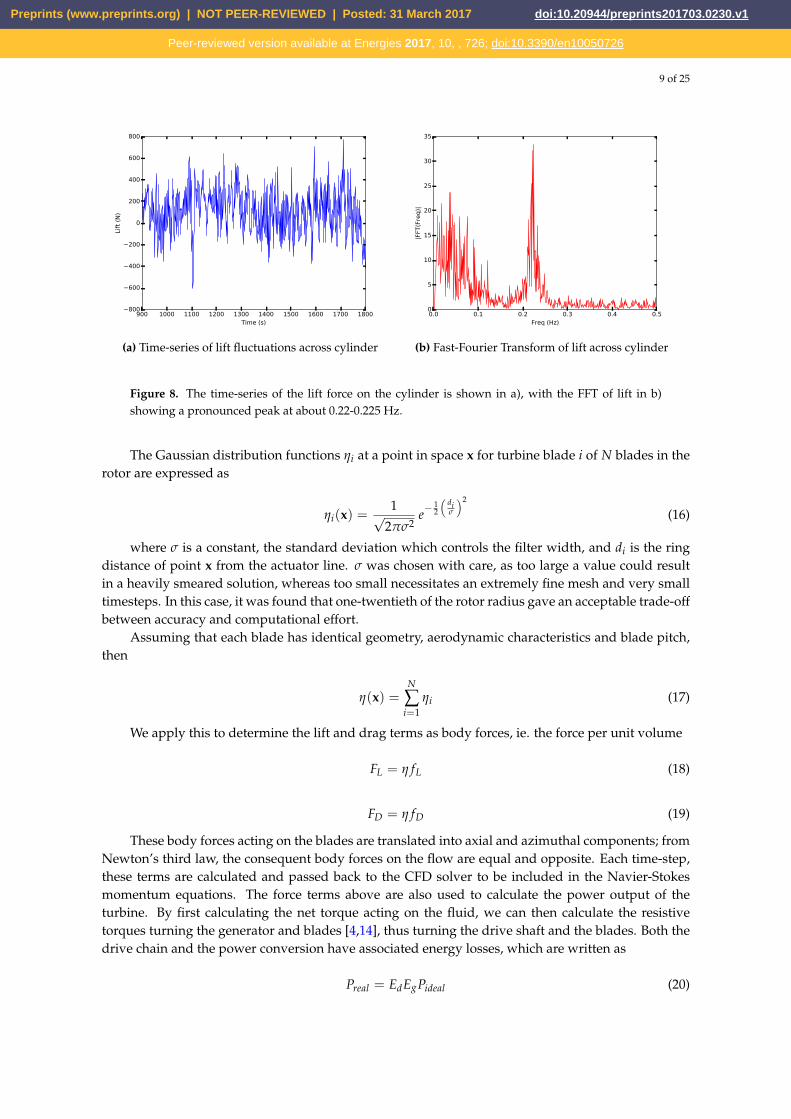
A fast-Fourier transform (FFT) was applied to the lift force fluctuations. The resulting powerspectrum in Figure 8b contains a sharp peak around 0.22-0.225 Hz. For uH = 2 ms−1, equation (13),this gives a Reynolds number of Re ≈ 3.37× 106, and a Strouhal number of St = 0.3300− 0.3375.Although this is above the values reported by Roshko [53] (St=0.26-0.28) and Shih et al. [46] (St=0.25),it falls within the lower limit of the measurements of Delany and Sorensen [44] who calculatedSt=0.32-0.45. This is within the accepted range of Strouhal numbers given in the literature, and so the




http://dx.doi.org/10.3390/en10050726

8 of 25

Figure 6. Horizontal slice through the velocity field at z=16 m and t=900s, showing the full extent ofthe wake behind the cylinder at the scale of the channel.

Figure 7. Horizontal slice through the vorticity field at z=16 m and t=900 s, showing the vorticitygenerated by flow past the cylinder.

combination of cylinder surface mesh resolution and quadratic skin friction coefficient was deemedsufficient for simulation of realistic wake effects.

3. Turbine formulation

The turbine model developed here builds upon previous work, where dynamictorque-controlled actuator discs with active-pitch correction were used to model wind turbines[14] and wind farms [4,15]. In the present model, actuator line techniques [5] have been used torepresent the rotor, whereby the blades themselves are not resolved, but the forces exerted by themon the fluid are still present. In actuator line theory, the blade is replaced by the actuator line, and theforces are spread spatially via a normalised Gaussian distribution function to become body forces. Inthis implementation, we use a two-dimensional Gaussian distribution function, which is describedbelow. The code for the model has been released as open-source, under the Lesser GNU PublicLicense, version 2.1 [54].

3.1. Methodology

The lift and drag force components per unit span acting on a blade are given by

fL = CL(α, Re)12

ρu2relc(r) (14)

fD = CD(α, Re)12

ρu2relc(r) (15)

where CL(α, Re) and CD(α, Re) are the coefficients of lift and drag respectively, both functions ofangle of attack α and Reynolds number Re; ρ is the density of the fluid (for a tidal turbine, seawater)in which the blades move; urel is the relative speed of the fluid over the blades; and c(r) is the chordthickness as a function of r, the radial distance from the hub centre.




http://dx.doi.org/10.3390/en10050726

9 of 25

900 1000 1100 1200 1300 1400 1500 1600 1700 1800Time (s)

800

600

400

200

0

200

400

600

800

Lift

(N

)

(a) Time-series of lift fluctuations across cylinder

0.0 0.1 0.2 0.3 0.4 0.5Freq (Hz)

0

5

10

15

20

25

30

35

|FFT

(Fre

q)|

(b) Fast-Fourier Transform of lift across cylinder

Figure 8. The time-series of the lift force on the cylinder is shown in a), with the FFT of lift in b)showing a pronounced peak at about 0.22-0.225 Hz.

The Gaussian distribution functions ηi at a point in space x for turbine blade i of N blades in therotor are expressed as

ηi(x) =1√

2πσ2e−

12

(diσ

)2

(16)

where σ is a constant, the standard deviation which controls the filter width, and di is the ringdistance of point x from the actuator line. σ was chosen with care, as too large a value could resultin a heavily smeared solution, whereas too small necessitates an extremely fine mesh and very smalltimesteps. In this case, it was found that one-twentieth of the rotor radius gave an acceptable trade-offbetween accuracy and computational effort.

Assuming that each blade has identical geometry, aerodynamic characteristics and blade pitch,then

η(x) =N

∑i=1

ηi (17)

We apply this to determine the lift and drag terms as body forces, ie. the force per unit volume

FL = η fL (18)

FD = η fD (19)

These body forces acting on the blades are translated into axial and azimuthal components; fromNewton’s third law, the consequent body forces on the flow are equal and opposite. Each time-step,these terms are calculated and passed back to the CFD solver to be included in the Navier-Stokesmomentum equations. The force terms above are also used to calculate the power output of theturbine. By first calculating the net torque acting on the fluid, we can then calculate the resistivetorques turning the generator and blades [4,14], thus turning the drive shaft and the blades. Both thedrive chain and the power conversion have associated energy losses, which are written as

Preal = EdEgPideal (20)




http://dx.doi.org/10.3390/en10050726

10 of 25

Table 1. General specifications for modelled turbine.

Property Symbol Value

Rotor radius R 8 mHub height zH 16 mRotor separation 26 mAerofoil type NACA 63-415Hub fraction rH/R 0.1Blade material density 1027 kg m−3

Cut-in wind speed uc_in 0.5 ms−1

Cut-out wind speed uc_out 5 ms−1

Design tip-speed ratio λ 4.5Rated flow speed urat 2.5 ms−1

Thrust at rated flow speed Trat 600 kN per rotor

where Preal is the actual power, Pideal is the ideal power without energy losses, Ed is the drivetrain efficiency, and Eg the generator and power conversion efficiency. We used Ed = 0.94, and Eg =

0.96, the values specified in Bedard [55] for the MCT/Siemens’ SeaGen device. An active pitchingalgorithm was used which maximises total lift, matching the behaviour of SeaGen [56]. Further detailsof the numerical model can be found in Creech et al. [4].

3.2. Parameterisation

The rotor configuration was based upon that of Marine Current Turbine’s SeaGen device [57], ie.dual rotors, aligned horizontally. As many of SeaGen’s technical details are commercially sensitiveand not readily available, rotor and performance specifications were sourced from journal papers[52,55,57–60]. Details often disagreed between papers, so discretion was applied in deciding on thevalues listed in Table 1. To validate the chosen parameters, candidate models were tested againstperformance data from SeaGen, as shown in Figure 9.

The aerofoil chosen was a NACA 63-415 type, which has desirable lift characteristics. The liftand drag at limited angles of attack were taken from previous work [4], which based its aerofoil dataon that from the Airfoil Catalogue [61]. Blade geometry was completely unknown, so as a startingpoint, the equation for the predicted flow angle at a turbine rotor was taken from Burton et al. [62]:

tan φ(r) =1− 1

3

λµ(

1 + 23λ2µ2

) (21)

where φ is the predicted inflow angle as a function of radial distance r, λ is the design tip-speedratio, and µ = r

R , where R is the radius of the turbine rotor. If the optimum angle of attack for a givenblade αopt, then the blade twist can be given as

β(r) = φ(r)− αopt (22)

αopt was calculated from the lift and drag coefficient charts for the chosen aerofoil type, as perCreech et al. [4]. This then provided the blade twist angles along the blade.

No information was available on chord thickness, so this was calculated using the equation foran ideal optimised blade derived from blade-element theory [62, Chapter 3], ie.

σrλCL,opt =89√(

1− 13

)2+ λ2µ2

[1 + 2

9(λ2µ2)

]2(23)




http://dx.doi.org/10.3390/en10050726

11 of 25

Figure 9. Time-averaged power (blue) and thrust (red) for a single rotor of SeaGen, as a function ofmean hub-height flow speed uH . The solid lines represent data sourced from Douglas et al. [59] andFraenkel et al. [52,57]; the squares and triangles represent simulation results.

where σr = Nc2πr is the rotor solidity (N is the number of blades, c the local chord thickness),

µ = r/R, and CL,opt is the lift coefficient at optimal operation, which is calculated from lift and dragperformance data. Rearranging gives

c(µ) =2πµR

NλCL,opt. X(µ) (24)

where X(µ) is the right-hand side of (23). The chord length can now be defined as a function ofr for a blade with specified characteristics.

3.3. Test cases and results

Test cases were devised to check that the specification of the rotor, the blades, and the generatorproperly represented the real tidal turbine, in a channel flow uH = 2 ms−1. To lessen computationalrequirements, a single rotor would be tested in a simulation domain much smaller than the emptychannel test case, measuring 250 m x 100 m x 30 m. No support structure was included to furtherreduce the number of elements required. The turbine rotor was positioned much closer to the inlet, at[50 m, 50 m, 16 m]. Such a short domain was acceptable because only the performance of the turbineswas of interest, and the wake effects could be ignored. In the final simulations, the turbine rotorswould be operating at below the rated power, so only hub-height flow speeds below 2.5 ms−1 wouldbe tested. Three mean hub-height flow speeds were considered: uH = {1, 1.5, 2}ms−1.

Figure 9 compares the resulting mean power and thrust from each case with publishedperformance data. The model yields slightly larger time-averaged values for power and thrust atuH = 1 ms−1 when compared to the published data, but it is in good agreement for both power andthrust when uH is at 1.5 and 2 ms−1, to within a maximum relative error of 8.8%. The cause of theover-performance of the model at the lowest flow speed could be down to minor discrepancies inthe rotor, blade or generator specifications, but this cannot be confirmed. Other possible causes maybe rotor-rotor wake interaction in the dual rotor configuration; this will be examined in Section 4.Notwithstanding this, the results provide reasonable confidence in the modelled rotor performanceat the target hub height flow speed of uH = 2 ms−1.




http://dx.doi.org/10.3390/en10050726

12 of 25

4. Full-scale turbine simulations

4.1. Overview

The simulations were based upon the tidal channel test case in Section 2.2, as it was sufficientlylarge (1 km x 200 m x 30 m) to allow realistic turbulence structures to develop, and to capture theextents of the turbine and structure wakes. To isolate and analyse the contributions of the variouscomponents of the turbine to the downstream wake, three different scenarios were considered: a)with dual contra-rotating rotors and no structure, b) with the complete support structure only, andc) with both the rotors and the structure present. For each of these scenarios, the mean hub-heightflow speed was set to uH = 2.0 ms−1, with turbulent inflow conditions provided via the syntheticeddy method used in Section 2.2.1. These simulations were run until the turbulent flow was fullydeveloped, and statistical properties of the flow, such as turbulence intensity and time-averaged flowspeeds, had become stable; this was a minimum of 2700 s in all runs. Each simulation was then runfor a further 900 s, during which full sets of data for the velocity and pressure were saved to disc foranalysis each second for post-processing. At the time the computations were undertaken, Fluiditydid not support the use of point detectors (probes) when running in parallel, and so higher frequencysampling of velocity fields for spectral analysis was not possible. Nevertheless, the 900 s samplingperiod was sufficient to provide time-averaged velocity profiles that appeared to be statisticallystationary. All simulations were run on ARCHER, the UK’s national academic supercomputer, using2400 computing cores each of which typically used 1.5 MAUs of allocation units, with a wall time of2-3 days.

4.2. Configurations

The support structure model is shown in Figure 10, which was based upon SeaGen’s design. Themodel consists of a 30 m high, 3 m diameter monopile that pierces the water surface, with a crossbeamat a height of 15 m above the sea bed. The crossbeam is 27 m broad, and 4 m long, encompassing themonopile, and contains angled sections on either side, that rise 1 m and taper to 3 m long at theirfurthest extent. Solid nacelle sections measuring 1 m x 3 m x 2 m are located at the ends of thecrossbeam. The crossbeam edges have been smoothed to have a curved surface of radius 0.5 m, ashave the nacelles. This arrangement closely follows details given by Fraenkel [52], Neill et al. [60]and Fraenkel [57], whilst also taking cues from Keenan et al. [36]. The more complex quadropodbase was not adopted in the final design, due to the prohibitive mesh refinement and complexity thatwould have been required. The structure was placed on the seabed in the empty rectilinear channeldescribed in Section 2.2, such that the monopile base was centred at [250 m, 100 m, 0 m].

The contra-rotating rotors case used the design developed in Section 3.2. They were positioned infront of the solid nacelle structures, with the first rotor T1 at [247 m, 87 m, 16 m], and the second rotorT2 at [247 m, 113 m, 16 m]. The blades were oriented on T1 and T2 so that the lift-induced torquewould cause clockwise and anti-clockwise rotations respectively, thus forming the contra-rotatingpair shown in Figure 11. Each rotor was connected to a modelled generator, and like SeaGen, thesegenerators operated asynchronously [63]. The mesh resolution was highest near the blades andreduced gradually with distance from the rotors, as can be seen in Figure 12.

The final case combined the dual rotors and structure configurations above. Table 2 lists themesh resolutions and time-step sizes for each case.

5. Results

This section examines the time-averaged velocity and turbulence intensity data obtained fromthe full simulations of turbulent flow in the rectilinear channel with the dual rotors, with thesupporting structure on its own, and with both the dual rotors with the support structure. Even with




http://dx.doi.org/10.3390/en10050726

13 of 25

Figure 10. The turbine structure: a) a perspective view illustrating the main components, and b) ahead-on view indicating important dimensions.

Figure 11. Contra-rotating rotors with centres separated by 26 m.

Figure 12. Horizontal slice at hub height through the mesh for the dual rotors only case. Meshresolution increases sharply toward the rotors, and reduces gradually downstream to the resolutionused in the empty channel case.

Table 2. Simulation configuration details.

Parameter Rotors Structure Rotors+structure

∆t (s) 16

16

16

Min. mesh res. (m) [0.5, 0.5, 0.5] [0.25, 0.25, 0.25] [0.25, 0.25, 0.25]Max. mesh res. (m) [2, 2, 0.5] [2, 2, 0.5] [2, 2, 0.5]Mesh cells (106) 31.9 30.4 38.7




http://dx.doi.org/10.3390/en10050726

14 of 25

the aforementioned limitations in sampling time and frequency, the results give a good qualitativerepresentation of the persistent flow features.

5.1. Wake effects

Here, the difference in the wake effects between each of the three cases are considered: rotorsonly, structure only, and rotors+structure. Two sets of profiles are examined: i) cross-stream (ortransect) profiles at rotor hub height zH ; and ii) vertical profiles, on vertical streamwise planes slicingthrough both rotor hubs at y = {87, 113}m. Both sets of profiles are from x=-1 D upstream to 20 Ddownstream. These are augmented by selected instantaneous velocity slices over the full length ofthe domain (≈47 D downstream).

From the time-averaged velocity profiles for the rotors-only case in Figure 13a, it is clear thatby x=20 D, the flow has almost fully recovered to its upstream profile, uH(x = 20 D) having 90% ofits upstream value (denoted u0). Immediately downstream of the rotors at 1 D, the deficit matchesclosely the zone swept out by the blades, beginning at zt=24 m (top of the rotor) and ending at zb=8 m(bottom of the rotor). In the absence of a nacelle, the flow passes through the hub section (z=15.2-16.8m) relatively unimpinged, peaking at 0.85 u0. This hub-section flow is still evident at 5 D, but by 10D has decayed into a quasi-Gaussian deficit. Upstream of the rotors, the vertical profile of turbulenceintensity (TI) is similar to that in the undisturbed channel (Figure 4c); downstream it peaks at the hubsection and the rotor tips, indicating the presence of tip-vortex shedding. The TI profile maintainsthis general shape until 10 D, whereupon it starts to begins to decay. By 20 D however, the TI valuesremain higher than the original upstream profile. The horizontal velocity transect at hub height inFigure 14a shows a similar pattern, with the same mid-rotor peaks at y={87, 113} m, which eventuallybecome smoothed troughs by 10 D. In the area between the rotors the flow speed increases to 2.2ms−1, due to blockage by the rotors and the absence of the support structure. Asymmetry occurs inthe rotor deficits from 1-5 D, with the radially-inward tip deficits 0.2 ms−1 higher than the outward tipdeficits. The accelerative effect of the rotor blockage plays an important role here: in the instantaneousvelocity field snapshot Figure 15a, there is a jetting phenomenon between the rotors. This has alsobeen noted in previous work modelling offshore wind farms [4]. The TI plots also exhibit peaks atthe rotor tips and the hub section from 1D onwards; these persist even at 20 D, and do not decay toupstream levels.

For the structure-only case (Figures 13c and 14c), the velocity profiles show a sharp dropimmediately behind the crossbeam, with nearly full velocity recovery by 5 D. The horizontal-transectprofiles are more complicated, as the transect is at hub-height (z=16 m), and crosses in front of (andbehind) the tower, as well as the upper, outer ends of the crossbeam (cf. Figure 10). Furthermore,the nacelles exert a strong influence on turbulence levels, raising the TI to 17.5% at 1 D, 13% at 5 D,before approaching background levels by 10 D. At 20 D, the difference between upstream TI valuesis negligible.

The velocity profiles for the rotors+structure case (Figures 13c and 14a) are broadly similar tothe rotors-only case, but with several important differences. Firstly, the pronounced peak visiblein the rotors-only profile (Figure 13a and 14a) has been replaced with flatter troughs. This is dueto the influence of the crossbeam and the nacelle sections, causing the flow to accelerate aroundthe solid structure, rather than through the empty hub volume in the rotors as before. This effectcan be observed in the instantaneous vertical velocity snapshots in Figures 15c and 15d (zoomedin). Secondly, the flattened velocity peak in the horizontal transects between the rotors no longeroccurs at 1D, owing to the presence of the monopile and crossbeam. Instead, two sharp spikes canbe seen at approximately u0, either side of the central trough at 0.8 ms−1. By 5 D downstream, thesehave become one peak at 1.8 ms−1, somewhat lower than in the rotors case (2.2 ms−1). This patterncontinues at 10 D and 20 D; the velocity profiles similar but ≈ 0.1− 0.2 ms−1 lower in the rotors andstructure regions. The horizontal velocity snapshot in Figure 15b reflects this, with the pronouncedcentral jet between the rotor wakes in Figure 15a no longer visible. As expected, the vertical TI profile




http://dx.doi.org/10.3390/en10050726

15 of 25

(a) Rotors (b) Structure (crossbeam) (c) Rotors+structure

Figure 13. Vertical profiles of time-averaged velocity magnitude and turbulence intensity for rotors,structure, and rotors with structure. The units for x are D, ie. the rotor diameter (=16 m).

(a) Rotors

(b) Structure

(c) Rotors with structure

Figure 14. Horizontal transects of time-averaged velocity and turbulence intensity at z=16 m for eachfull-scale case. Units for x are D.




http://dx.doi.org/10.3390/en10050726

16 of 25

Table 3. Comparison of power output values

Case Power (kW) % Error

Measured (both rotors) 750.0 -Single rotor (x2) 711.4 5.147T1 + T2 rotors 784.5 4.398T1 + T2 rotors with structure 786.6 4.653

in Figure 13c is broadly similar to that in Figure 13a, but higher turbulence levels occur downstream,particularly behind the structure. At 1 D, the TI is between 20-25% near the nacelle region, muchhigher than the 12-17% for the rotors only. By 10 D however, TI profiles from both the rotors-only androtors+structure cases are nearing equivalence. Lastly, of particular note are the TI peaks at the rotortips, visible in Figures 13c and 14c, which are 16-40% larger than the rotors case. This suggests thatthe blades themselves may be subject to, and causing, fluctuations in the flow. Turbulence spectrawere calculated at a point 1 D downstream from top of rotor T1 for both cases (cf. Figure 16), whichconfirm that while both exhibit a peak at 0.4 Hz, this is particularly pronounced when the structureis included. We explore this further in Section 5.2.

5.2. Turbine diagnostics

Here we examine how the performance of the turbine is affected by the absence or inclusion ofthe support structure. Figure 17 presents a selection of diagnostics from the rotors-only test, whichshow that the power from each rotor fluctuates semi-independently of the other, due to the unsteady,turbulent flow each rotor experiences. We use the term ‘semi-independently’, because some of theeddies are large enough for each rotor to experience them simultaneously. For both rotors T1 and T2,power output varies approximately ±25 kW from their mean values. The mean power outputs forT1 and T2 differ by 0.25%; for simulations of longer duration these should converge. The weightedangle of attack along the blades, α, shows much less variation, as the pitch control mechanism tries tomaximise power output [4,56]. The results from the rotors + structure case are broadly similar.

The net time-averaged power output of cases for the single rotor, both rotors only, and thenthe rotors+structure are compared against published measurements for SeaGen in Table 3. Themodels are in close agreement, with a maximum error of 5.147%. It is particularly interesting thatthe simulations modelling both rotors have more accurately predicted the power output than thesingle rotor case, suggesting that there is interaction between the two rotors. This may be down tothe blockage effects of each individual rotor, which accelerates flow round the edges of the rotors, intheory providing a small performance increase. Indeed, the acceleration effect can clearly discerniblein Figure 14a.

Investigating the effect of the support structure on the power output, Table 3 indicateslittle difference between the rotors and rotors+structure cases, with errors of 4.398% and 4.653%respectively. It is also worth examining the time-series of the power output from each rotor, to see ifthere are any regular fluctuations as the blades pass in front of the supporting structure (such as thecrossbeam).

This was achieved by applying Fast-Fourier transforms (FFT) to the power output. As there wasa short sampling period (900 s), and the likelihood of similar spectral characteristics in fluctuationsin each rotor, for each simulation, FFTs of the power time-series for each rotor were calculatedseparately, and then the average of them taken. Figure 18 displays these for the rotors case andthe rotors+structure case. Towards the lower end of the frequency range both plots become noisy,as longer wavelengths are not resolved satisfactorily within the sampling period. In Figure 18a, therotors only case, there is a small peak at 0.4 Hz; however in Figure 18b, when the structure is added,the peak at the same frequency is much larger. The mean rotational frequency of the rotors in onesimulation is defined as




http://dx.doi.org/10.3390/en10050726

17 of 25

(a) Rotors case horizontal slice at hub height.

(b) Rotors+structure case horizontal slice at hub height.

(c) Rotors+structure case vertical slice through hub of rotor T1.

(d) Zoomed-in rotors+structure case vertical slice through hub of rotor T1.

Figure 15. Instantaneous snapshots of the velocity field for rotor and rotor+structure cases, at the endof the simulation.




http://dx.doi.org/10.3390/en10050726

18 of 25

0.0 0.1 0.2 0.3 0.4 0.5Rotors: Freq (Hz)

0.000

0.005

0.010

0.015

0.020

0.025

Roto

rs:

|FFT

(Fre

q)|

(a) Rotors only

0.0 0.1 0.2 0.3 0.4 0.5Rotors+struct: Freq (Hz)

0.000

0.005

0.010

0.015

0.020

0.025

Roto

rs+

stru

ct:

|FFT

(Fre

q)|

(b) Rotors+structure

Figure 16. Resolved turbulence spectra at 1D downstream from the top of the T1 rotor, for a) the rotorscase, and b) rotors+structure. Both cases show a second peak at 0.4 Hz, with the peak 4 times higherin the rotors+structure case.

Figure 17. Diagnostic output from both rotors, T1 and T2, showing power, and α, the weighted meanangle of attack (see Creech et al. [4] for details) for each. The dashed lines indicate mean power output.




http://dx.doi.org/10.3390/en10050726

19 of 25

Table 4. Mean rotational frequencies of the rotors in each simulation case.

Case ωC rad s−1) fC (Hz)

Rotors 1.255 0.1997Rotors+structure 1.255 0.1997

Table 5. High frequency power fluctuation ranges for rotor and rotor+structure cases.

Case Fluctuation range (Pmax − Pmin) (kW) % mean rotor power

Rotors 5.0 1.3Rotors+structure 15.0 3.8

fC =ωC2π

=1

2π(|ω|T1 + |ω|T2) (25)

where ωTn is a time-averaged rotor angular velocity from the diagnostics data for rotor Tn.The values for the frequencies in Table 4 demonstrate that both cases are identical to within four

significant figures. It should be noted that fC is almost exactly half of 0.4 Hz, shown in Figures 18aand 18b. This is not surprising, given there are two blades. To determine where in the rotation cyclethese high-frequency power fluctuations occur, the low frequencies were removed using a Hammingwindow function, with spectral inversion used to create a high-pass filter. The cutoff frequency was0.3 Hz, with a transition bandwidth of 0.05 Hz. The position of the first blade was then plotted againstthese fluctuations for each turbine. For comparison, the same process was carried for the case withrotors only, and the graphs for both are shown in Figure 19.

Figure 19a shows that in the rotors-only case, the power fluctuations have a relatively evenspread within a range of ± 2.5 kW, with slightly higher values when either blade points upwardsat 0◦. This increase is most likely due to the higher flow speeds and thus the lift which the bladesexperience at 0◦, as shown in the vertical velocity profile in Figure 13a. Discrepancies between thisand the rotor+structure case are quite evident from Figure 19b, where a clear pattern emerges, withfluctuations peaking at a maximum of 7.5 kW at a blade position of 0◦ and 180◦, and at a minimum of-7.5 kW at 90◦ and 270◦. Table 5 lists these in terms of mean total output per rotor. It is clear that in therotors+structure simulation, a dip in power output is experienced when the blades are aligned withthe cross-beam. By comparing the horizontal velocity profiles at hub height in Figures 14a and 14c,just downstream of the rotors at x=1 D, the velocity deficits are more pronounced when the structureis included. In particular, the absence of the nacelles and tower is noticeable, with peaks flow speedof 1.75 ms−1 in the rotors-only case at y=87 m and y=113 m, and at y=100 m, where the nacelles andtower would be, respectively. This can be attributed to the blockage effect, created by the back thrustof the rotors, causing the flow to accelerate around the rotors and through the centre where the lift isreduced. In contrast, the velocity profiles in Figure 14c show no accelerated flow at the nacelles, andthe velocity deficit created by the wake of the tower reaches 0.8 ms−1, compared to the rotors-onlycase, which peaks at 2.2 ms−1, ie. 1.1 u0. The culmination of the upstream effect of the supportingstructure, in terms of the turbine performance, is a periodic fluctuation in power, responsible for avariation in output of almost 4%.

6. Discussion and conclusions

Large Eddy Simulation has been used to model a full-scale, dual rotor, contra-rotatingturbine, complete with structure, in a realistic-sized channel domain. The results demonstrate thatthe structure does have a noticeable effect on performance and the near-wake, causing regularfluctuations in both power output and flow speed.




http://dx.doi.org/10.3390/en10050726

20 of 25

0.0 0.1 0.2 0.3 0.4 0.5Rotors: Freq (Hz)

0

500

1000

1500

2000

2500

3000

3500

4000

4500

Roto

rs:

|FFT

(Fre

q)|

(a) Rotors only

0.0 0.1 0.2 0.3 0.4 0.5Rotors+structure: Freq (Hz)

0

500

1000

1500

2000

2500

3000

3500

4000

Roto

rs+

stru

cture

: |F

FT(F

req)|


Figure 18. Rotor-averaged FFT plots of the power time-series, for (a) rotors only, and (b)rotors+structure. There is a pronounced spike at 0.4 Hz for the simulation that includes the supportstructure.

0°

45°

90°

135°

180°

225°

270°

315°

-5-2.5

02.5

57.5 kW

T1T2

(a) Rotors only

0°

45°

90°

135°

180°

225°

270°

315°

-5-2.5

02.5

57.5 kW

T1T2


Figure 19. Polar plots of blade position versus power fluctuations above 0.3 Hz, for rotors T1 and T2,in (a) the rotors-only simulation, and (b) including the structure. 0◦ means the blade is pointingupwards, and power fluctuations are plotted from -7.5–7.5 kW. T1 rotates anti-clockwise, and T2rotates clockwise. The extent of the power fluctuations is approximately ± 7.5 kW in (b), whereasin (a) it is a third of the size, at ± 2.5 kW.




http://dx.doi.org/10.3390/en10050726

21 of 25

There are few CFD models of dual rotor configurations in modelling literature. Of these, thetidal turbine array LES simulations of Churchfield et al. [8], show similarities in the downstreamwake profiles; however their domain was less than a quarter of the size of the channel domain usedhere, and so their results may be subject to exaggerated blockage effects due to proximity of thedomain walls. Furthermore, they did not use synthetic eddy methods for realistic inlet turbulence,unlike the present paper. Closer comparisons may be drawn with Afgan et al. [26] and Ahmedet al. [27], who used k − ω SST RANS, and also LES with SEM to model a resolved three-bladedrotor and the support structure. Their time-averaged LES results of the power coefficient exhibitedregular pronounced fluctuations as a function of blade angle with the rotors upstream; in the RANSsimulations these were absent. The RANS models of Mason-Jones et al. [64] however, did predictincreased fluctuations in torque with blade angle when the stanchion supporting the turbine wasincluded. The lesson here is that care must be used when deploying RANS turbulence schemes tocapture transient behaviour in diagnostics. Moreover, the flow direction experiments of Frost et al.[65] showed that individual blade thrusts varied considerably with blade angle upstream, whereasnet rotor thrust and power output did not. It must be noted that their turbine configuration differssomewhat from our model, having 3-blades with one central monopile, versus our dual two-bladed,crossbeam-mounted arrangement. Although there are valuable advances in research using actuatordisc approaches [23,25,66,67], particularly in terms of tidal farm modelling, the discretisation ofthe blades into continuous rings means that such models cannot capture the same fluctuations inpower output due to blade-structure interaction. Whether or not this is important for the far-wake oftidal turbines remains an open question, but for mechanical and electrical reliability, these transientfeatures must either be represented or parameterised for accurate simulation.

In terms of wake prediction, measurements from a full-scale turbine would have been useful formodel validation. As with the technical specifications however, ADCP measurements of SeaGen’sdownstream wake were unavailable, so comparison is instead made with the experimental andnumerical literature. The water channel tests of Myers and Bahaj [68], despite being of scaledsingle rotor turbine, support the results in Figures 13b and 14c, that show the structure alone createssubstantial turbulence even at 5 D downstream. With the rotors included, our findings agree withthose of Batten et al. [24], and Stallard et al. [69,70], in that at 20 D (22 D in Batten), the turbinewake had still not recovered to its original value. They too report higher than background readingsfor turbulence intensity far downstream. In the near wake, there is good agreement between thecross-stream turbulence profile in Figure 14c and Tedds et al. [71], both showing peaks of 20-25% 1-2D downstream, as well a peak at the centre near the structure. This is surprising, given the differencesin geometry of both rotor and structure; indeed the difference in structure (single stanchion versusmonopile+crossbeam for SeaGen) may account for the variance in the central peak. Such conformanceacross a range of scales and models is encouraging, given that levels of upstream turbulence havebeen found to influence tidal turbine performance [72]; the turbulence profiles in our rectilinearchannel reflect a satisfactory approximation to a generic channel, but they do not reflect any particulartidal site.

The key finding of this paper is that the support structure has a discernible effect on the flowupstream, the downstream wake, and turbine behaviour, for a contra-rotating, dual rotor tidalturbine. The behavioural changes manifest themselves as regular oscillations in the power output attwice the rotor rotational frequency, and constitute 4% of total output. Furthermore, these fluctuationsaffect the near-wake of each rotor, where these oscillations are evident in the turbulence spectra,and so undoubtedly causing regular variations in structural loading. Inclusion of the structure insimulations also produces deeper, more persistent wake deficits, as well as substantially higher levelsof turbulence downstream, well into the far wake. This bears further investigation, particularlyfor tidal turbine arrays. It is recommended that future work should be undertaken to investigatethe consequences of such complicated wake flows, for the electrical and mechanical systems oftidal turbines. In summary, the present study confirms that if the support structure and individual




http://dx.doi.org/10.3390/en10050726

22 of 25

rotors are not resolved or parameterised appriopriately within a numerical model, then the resultsof such simulations should be held in doubt, from the interrelated perspectives of turbine reliability,performance and fluid dynamics.

Acknowledgments: This research was supported through NERC (UK) grant NE/J004332/1 on the jointproject ‘FLOWBEC - FLOW and Benthic ECology 4D’, with additional support from EPSRC(UK), grantref. EP/M014738/1 ‘Extension of UKCMER Core Research, Industry and International Engagement’. Wealso acknowledge the support of 10 MAUs of computing time on ARCHER, the UK national academicsupercomputer. Finally, we would like to thank Peter Fraenkel for his invaluable contributions and insightsinto tidal turbine design.

Author Contributions: A.C.W. Creech conceived the research, designed and ran the simulations, analysed thedata, and wrote the paper; A.G.L. Borthwick contributed ideas to the research; A.G.L. Borthwick and D. Ingramcontributed revisions to the paper.

Conflicts of Interest: The authors declare no conflict of interest.

References

1. Jensen, N. A note on wind generator interaction. Technical report, Risø National Laboratory, Roskilde,Denmark, 1983.

2. Jimenez, A.; Crespo, A.; Migoya, E.; Garcia, J. Large-eddy simulation of spectral coherence in a windturbine wake. Environmental Research Letters 2008, 3(1), 015004.

3. Wu, Y.T.; Porte-Agel, F. Large-Eddy Simulation of Wind-Turbine Wakes: Evaluation of TurbineParametrisations. Boundary-Layer Meteorology 2011, 138, 345–366.

4. Creech, A.C.W.; Früh, W.G.; Maguire, A.E. Simulations of an offshore wind farm using large eddysimulation and a torque-controlled actuator disc model. Surveys in Geophysics 2015, 36, 427–481.

5. Sørensen, J.; Shen, W. Numerical modelling of wind turbine wakes. Journal of Fluids Engineering 2002,124, 393–399.

6. Troldborg, N.; Sorensen, J.; Mikkelsen, R. Numerical simulations of wake characteristics of a wind turbinein uniform inflow. Wind Energy 2010, 13, 86–99.

7. Churchfield, M.J.; Lee, S.; Moriarty, P.J.; Martínez, L.A.; Leonardi, S.; Vijayakumar, G.; Brasseur, J.G. ALarge-Eddy Simulation of Wind-Plant Aerodynamics. 50th AIAA Aerospace Sciences Meeting, 2012.

8. Churchfield, M.J.; Li, Y.; Moriarty, P.J. A Large-Eddy Simulation Study of Wake Propagation and PowerProduction in an Array of Tidal-Current Turbines. Phil. Trans. R. Soc. A 2013, 371, 1471–2962.

9. Barthelmie, R.; Folkerts, L.; Rados, G.C.L.K.; Pryor, S.C.; Frandsen, S.T.; Lange, B.; Schepers, G.Comparison of Wake Model Simulations with Offshore Wind Turbine Wake Profiles Measured by Sodar.Journal of Atmospheric and Oceanic Technology 2006, 23, 888 – 901.

10. Sanderse, B.; van der Pijl, S.; Koren, B. Review of computational fluid dynamics for wind turbine wakeaerodynamics. Wind Energy 2011, 14, 799–819.

11. Creech, A.C.W.; Früh, W.G. Modelling wind turbine wakes for wind farms. Wiley Encyclopedia of Energy2016.

12. Wußow, S.; Sitzki, L.; Hahm, T. 3D-simulation of the turbulent wake behind a wind turbine. Journal ofPhysics Conference Series 2007, 75, 12036–12036.

13. Früh, W.G.; Seume, J.; Gomez, A. Modelling the aerodynamic response of a blade passing in front of thetower. European Wind Energy Conference, 2008.

14. Creech, A.C.W.; Früh, W.G.; Clive, P. Actuator volumes and hr-adaptive methods for 3D simulation ofwind turbine wakes and performance. Wind Energy 2012, 15, 847 – 863.

15. Creech, A.C.W.; Früh, W.G.; Maguire, A.E. High-resolution CFD modelling of Lillgrund Wind farm.Renewable Energy and Power Quality Journal 2013.

16. Adcock, T.; Draper, S.; Houlsby, G.; Borthwick, A.; Serhadlıoglu, S. The available power from tidal streamturbines in the Pentland Firth. Proc. R. Soc. A 2013.

17. Coles, D.S.; Blunden, L.S.; Bahaj, A.S. Resource Assessment of Large Marine Current Turbine Arrays. J.of Ocean Engineering 2013.

18. Plew, D.; Stevens, C. Numerical modelling of the effect of turbines on currents in a tidal channel – ToryChannel, New Zealand. Renewable Energy 2013, 57, 269–282.




http://dx.doi.org/10.3390/en10050726

23 of 25

19. Funke, S.; Farrell, P.; Piggott, M. Tidal turbine array optimisation using the adjoint approach. RenewableEnergy 2014, 63, 658–673.

20. Lawson, M.; Li, Y.; Sale, D. Development and verification of a computational fluid dynamics model of ahorizontal-axis tidal current turbine. 30th Intl. Conf. on Ocean, Offshore and Arctic Eng., 2011.

21. Shi, W.; Wang, D.; Atlar, M.; Seo, K.C. Flow separation impacts on the hydrodynamic performanceanalysis of a marine current turbine using CFD. Proc. IMechE, Part A: J. Power and Energy 2013,227, 833–846.

22. Creech, A.C.W. A three-dimensional numerical model of a horizontal axis, energy extracting turbine.PhD thesis, Heriot-Watt University, 2009.

23. Nishino, T.; Willden, R. Effects of 3-D channel blockage and turbulent wake mixing on the limit of powerextraction by tidal turbines. Int. Journal of Heat and Fluid Flows 2012, 37, 123–135.

24. Batten, W.M.J.; Harrison, M.; Bahaj, A.S. The accuracy of the actuator disc-RANS approach for predictingthe performance and wake of tidal turbines. Phil. Trans. R. Soc. A 2013, 371.

25. Masters, I.; Williams, A.; Croft, T.; Togneri, M.; Edmunds, M. A Comparison of Numerical ModellingTechniques for Tidal Stream Turbine Analysis. Energies 2015, 8, 7833–7853.

26. Afgan, I.; McNaughton, J.; Rolfo, S.; Apsley, D.D.; Stallard, T.; Stansby, P.K. Turbulent flow and loadingon a tidal stream turbine by LES and RANS. Int. J. of Heat and Fluid Flow 2013, 43, 96–108.

27. Ahmed, U.; Afgan, I.; Apsley, D.; Stallard, T.; Stansby, P.K. CFD Simulations of a Full-Scale Tidal Turbine:Comparison of LES and RANS with Field Data. EWTEC, 2015.

28. McNaughton, J.; Afgan, I.; Apsley, D.D.; Rolfo, S.; Stallard, T.; Stansby, P.K. A simple sliding-meshinterface procedure and its application to the CFD simulation of a tidal-stream turbine. Int. J. for NumericalMethods in Fluids 2014, 74, 250–269.

29. Piggott, M.; Pain, C.; Gorman, G.; Power, P.; Goddard, A. h, r, and hr adaptivity with applications innumerical ocean modelling. Ocean Modelling 2004, 10, 95–113.

30. Baliga, B.; Patankar, S. A New Finite-Element Formulation for Convection-Diffusion Problems. NumericalHeat Transfer 1980.

31. Smagorinsky, J. General Circulation Experiments with the Primitive Equations. Monthly Weather Review1963, 91:99.

32. Deardroff, J.W. A numerical study of three-dimensional turbulent channel flow at large Reynoldsnumbers. J. Fluid Mech. 1970, 41, 453–480.

33. Bull, J.R.; Piggott, M.; Pain, C. A finite element LES methodology for anisotropic inhomogeneous meshes.Turbulence, Heat and Mass Transfer 2012, 7.

34. Scotti, A.; Meneveau, C. Generalized Smagorinsky model for anisotropic grids. Phys. Fluids A 1993,5, 2306–2308.

35. Bentham, T. Microscale Modelling of Air Flow and Pollutant Dispersion in the Urban Environment. PhDthesis, Imperial College London, 2003.

36. Keenan, G.; C. Sparling, H.W.; Fortune., F. SeaGen Environmental Monitoring Programme. Technicalreport, Royal Haskoning, 2011.

37. Rippeth, T.; Williams, E.; Simpson, J. Reynolds Stress and Turbulent Energy Production in a TidalChannel. Journal of Physical Oceanography 2001, 32, 1242–1251.

38. Jarrin, N.; Benhamadouche, S.; Laurence, D.; Prosser, R. A synthetic-eddy-method for generating inflowconditions for large-eddy simulations. Int. Journal of Heat Fluid Flows 2006, 27, 585–593.

39. Nezu, I.; Nakagawa, H. Turbulence in Open Channel Flows; A.A. Balkema, 1993.40. Milne, I.; Sharma, R.; Flay, R.; Bickerton, S. Characteristics of the Onset Flow Turbulence at a Tidal-Stream

Power Site. 9th European Wave and Tidal Energy Conference, 2011.41. Stacey, M.; Monismith, S.; Burau, J. Measurements of Reynolds stress profiles in unstratified tidal flow.

Journal of Geophysical Research 1999, 104, 10933–10949.42. Bryden, I.G.; Couch, S.J.; Owen, A.; Melville, G. Tidal current resource assessment. Proc. IMechE, Part A:

J. Power and Energy 2007, 221, 125–135.43. Bearhop, S.; Elsasser, B.; Inger, R.; Pritchard, D., Marine Renewable Energy Technology and

Environmental Interactions; Springer, 2014; chapter Strangford Lough and the SeaGen tidal turbine, pp.153–172.




http://dx.doi.org/10.3390/en10050726

24 of 25

44. Delany, N.K.; Sorensen, N.E. Low-speed drag of cylinders of various shapes. Technical Report Technicalnote 3038, National Advisory Committee for Aeronautics, 1953.

45. Thom, A. The Forces on a Cylinder in Shear Flow. Technical report, Ministry of Aviation, 1963.46. Shih, W.; Wang, C.; Coles, D.; Roshko, A. Experiments on flow past rough circular cylinder at large

Reynolds numbers. Journal of Wind Engineering and Industrial Aerodynamics 1993, 49, 351–368.47. Mackwood, P.; Bearman, P.; Graham, J. Wave and current flows around circular cylinders at large scale; HSE

Books, 1998.48. Chaplin, J.; Teigen, P. Steady flow past a vertical surface-piercing circular cylinder. Journal of Fluids and

Structures 2003, 18, 271–285.49. Cabot, W.; Moin, P. Approximate Wall Boundary Conditions in the Large-Eddy Simulation of High

Reynolds Number Flow. Flow, Turbulence and Combustion 2000, 63, 269–291.50. Wang, M.; Catalano, P.; Iaccarino, G. Prediction of high Reynolds number flow over a circular cylinder

using LES with wall modeling. Technical report, Center for Turbulence Research, 2001.51. Ochoa, J.; Fueyo, N. Large Eddy Simulation of the flow past a square cylinder. PHOENICS 10th

International User Conference, 2004.52. Fraenkel, P. Marine current turbines: pioneering the development of marine kinetic energy converters.

Proc. IMechE, Part A: J. Power and Energy 2007, 221, 159–169.53. Roshko, A. Experiments on the flow past a circular cylinder at very high Reynolds number. Journal of

Fluid Mechanics 1961.54. Creech, A.C.W. GitHub source code repository for Wind And Tidal Turbine Embedded Simulator

(WATTES). Available online: https://github.com/wattes, 2017.55. Bedard, R. TP-004-NA: Survey and Characterization of TISEC Devices. Technical report, Electric Power

Research Institute, 2005.56. Fraenkel, P. Private communication, 2014.57. Fraenkel, P. Practical tidal turbine design considerations: a review of technical alternatives and key design

decisions leading to the development of the SeaGen 1.2MW tidal turbine. Ocean Power Fluid MachinerySeminar. IMechE, 2010.

58. Myers, L.; Bahaj, A.S. Simulated electrical power potential harnessed by marine current turbine arrays inthe Alderney Race. Renewable Energy 2005, 30, 1713–1731.

59. Douglas, C.A.; Harrison, G.P.; Chick, J.P. Life cycle assessment of the SeaGen marine current turbine.Proc. IMechE Part M: J. Engineering for the Maritime Environment 2008, 222.

60. Neill, S.; Couch, E.L.S.; Davies, A. The impact of tidal stream turbines on large-scale sediment dynamics.Renewable Energy 2009, 34, 2803–2812.

61. Bertagnolio, F.; Sørensen, N.; Johansen, J.; Fuglsang, P. Wind turbine airfoil catalogue. Technical ReportRisø-R-1280(EN), Risø National Laboratory, 2001.

62. Burton, T.; Sharpe, D.; Jenkins, N.; Bossanyi, E. Wind Energy Handbook; Wiley, 2006.63. MacEnri, J.; Reed, M.; Thiringer, T. Influence of tidal parameters on SeaGen flicker performance. Phil.

Trans. R. Soc. A 2013.64. Mason-Jones, A.; O’Doherty, D.; Morris, C.; O’Doherty, T. Influence of a velocity profile & support

structure on tidal stream turbine performance. Renewable Energy 2013, 52, 23–30.65. Frost, C.; Morris, C.; Mason-Jones, A.; O’Doherty, D.; O’Doherty, T. The effect of tidal flow directionality

on tidal turbine performance characteristics. Renewable Energy 2015, 78, 609–620.66. Hunter, W.; Nishino, T.; Willden, R. Investigation of tidal turbine array tuning using 3D

Reynolds-Averaged Navier-Stokes Simulations. Int. Journal of Marine Energy 2015, 10, 39–51.67. Olczak, A.; Stallard, T.; Feng, T.; Stansby, P.K. Comparison of a RANS blade element model for tidal

turbine arrays with laboratory scale measurements of wake velocity and rotor thrust. Journal of Fluids andStructures 2016, 64, 87–106.

68. Myers, L.; Bahaj, A.S. Near wake properties of horizontal axis marine current turbines. EWTEC, 2009.69. Stallard, T.; Collings, R.; Feng, T.; Whelan, J.I. Interactions between tidal turbine wakes: experimental

study of a group of 3-bladed rotors. Phil. Trans. R. Soc. A 2013, 371.70. Stallard, T.; Feng, T.; Stansby, P.K. Experimental study of the mean wake of a tidal stream rotor in a

shallow turbulent flow. Journal of Fluids and Structures 2015, 54, 235–246.




http://dx.doi.org/10.3390/en10050726

25 of 25

71. Tedds, S.; Owen, I.; Poole, R. Near-wake characteristics of a model Horizontal axis tidal stream turbine.Renewable Energy 2014, 63, 222–235.

72. Mycek, P.; Gaurier, B.; Germain, G.; Pinon, G.; Rivoalen, E. Experimental study of the turbulenceintensity effects on marine current turbines behaviour. Part I: One single turbine. Renewable Energy2014, 66, 729–746.

c© 2017 by the authors. Licensee Preprints, Basel, Switzerland. This article is an open accessarticle distributed under the terms and conditions of the Creative Commons Attribution(CC-BY) license (http://creativecommons.org/licenses/by/4.0/).



http://creativecommons.org/

http://creativecommons.org/licenses/by/4.0/.


http://dx.doi.org/10.3390/en10050726

effects of support structures in an les actuator line ... of a tidal turbine with contra-rotating...

Documents