effects of soil type and water flux on solute transport

Effects of Soil Type and Water Flux on Solute TransportJ. Vanderborght,* C. Gonzalez, M. Vanclooster, D. Mallants, and J. Feyen

ABSTRACTPrediction of solute transport in soils requires appropriate transport

models and model parameters. The most suitable solute transportmodel and its parameters are likely to depend on both soil type andwater flux. This dependency was investigated by means of transportexperiments that were carried out in three different soils (Plaggept,Hapludalf, and Glossudalf) for two water application rates (0.5 and1.0 cm d ~'). Solute concentrations were measured during the transportexperiment at six different depths in undisturbed soil monoliths (1.0-mlength, 0.8-m i.d.) using time domain reflectometry (TDK). For eachdepth, parameters of two solute transport models, (i) the convectivelognormal transfer function (CLT) model assuming stochastic-convec-tive solute transport or no solute mixing and (ii) the convective-dispersive (CDE) model assuming complete solute mixing, were de-rived. The transport in the Plaggept and Hapludalf soil was bettermodeled as a stochastic-convective process. Furthermore, solute trans-port in these two soils was very heterogeneous, resulting from consider-able differences in local advection velocity. In the Glossudalf soil, solutetransport was more homogeneous and characterized as a convective-dispersive process. The heterogeneity of solute transport in both Plag-gept and Hapludalf soils increased with the applied water flux. Thisincrease was more pronounced in the Hapludalf soil, as the higherwater flux resulted in a larger contribution of macropores to flow andtransport of solutes.

SUITABLE MATHEMATICAL MODELS and appropriate val-ues for flow and transport parameters are needed to

assess the impact of surface-applied agrochemicals onthe subsurface environment. Transport of solutes in soilshas been conceptualized in many different ways, leadingto a variety of mathematical models that are used topredict solute transport. Solute transport in a homoge-neous porous medium can be predicted by the CDE,which assumes complete mixing of solutes so that, in aplane transverse to the advection direction, no variationsof solute concentration exist. The CDE model is knownto give accurate predictions in uniform (repacked) soils(e.g., Wierenga and van Genuchten, 1989; Vancloosteret al., 1993). However, inaccurate predictions by theCDE model have often been attributed to the lack ofsolute mixing causing horizontal variations of soluteconcentration, which result, from differences in localadvection velocity.

At the pore scale, horizontal variations of solute con-centration result from slow exchange of solutes betweendifferent pore groups in which solutes are advected down-wards with different velocities. This is of particularimportance in structured soils with large pores betweenstructural elements or aggregates through which solute

J. Vanderborght, M. Vanclooster, D. Mallants, and J. Feyen, Inst, forLand and Water Management, Katholieke Universiteit Leuven, Vital De-costerstraat 102, 3000 Leuven, Belgium; and C. Gonzalez, UniversidadNacional de Colombia, Engineering Faculty, Programa Colciencias. Re-ceived 7 Sept. 1995. *Corresponding author ([email protected]).

Published in Soil Sci. Soc. Am. J. 61:372-389 (1997).

transport occurs, bypassing the soil matrix (Dyson andWhite, 1987; Mallants et al., 1994). For those cases,mobile-immobile models (van Genuchten and Wierenga,1976) or dual (multiple) domain models (Jarvis et al.,1991; Gerke and van Genuchten, 1993; Gwo et al.,1995) may be more appropriate to model solute transport.

At a larger scale (field scale), differences in the localadvection velocity result from spatial variability of mac-roscopic soil hydraulic properties (Biggar and Nielsen,1976; Bowman and Rice, 1986; Destouni et al., 1994).When horizontal variations of solute concentration arepresent, the average solute concentration can be modeledby the CDE model using an effective dispersion coeffi-cient that accounts for the variability of the advectionvelocity (Toride and Leij, 1996) and the exchange ofsolutes between different pore domains (Passioura,1971). However, when deviations of advection velocityare persistent with depth, the effective dispersion willscale with depth (concentration profiles as a function oftime at specific depths) or time (concentrations profilesas a function of depth at specific times) (Simmons, 1982).

An alternative for modeling solute transport in hetero-geneous soils is to make use of the stream tube conceptintroduced by Dagan and Bresler (1979). Solutes arethen assumed to move in different stream tubes withoutany mixing of solutes between different stream tubes. Ifeffects of local-scale dispersion on solute transport canbe neglected, transport can be described entirely by theadvection velocity pdf from which the solute travel timepdf can be derived. A specific stream tube model usinga lognormal travel time pdf is the CLT model introducedby Jury (1982) and generalized for different concentrationmodes and boundary or initial conditions by Jury andScotter (1994). For several field-scale solute transportexperiments, the CLT model was successfully used topredict observed BTCs (Jury et al., 1982; Butters andJury, 1989). However, as was pointed out by Destouniet al. (1994), Toride and Leij (1996), and Mallants etal. (1996, unpublished data), neglecting the dispersionin the stream tubes results in an underestimation ofthe field-scale dispersion, especially close to the inputsurface. Furthermore, a stream tube model assumes avertically homogeneous soil and may therefore not beapplicable in most soils having different layers. To com-pensate for the effect of vertically varying soil watercontent, Ellsworth and Jury (1991) successfully usedtransformed depth coordinates. Therefore, a stream tubemodel using transformed depth coordinates may accu-rately predict solute transport in layered soils. However,at the boundary between two horizons, considerable sol-ute mixing may occur so that the concept of indepen-

Abbreviations: TDR, time domain reflectometry; CLT, convective lognor-mal transfer function; CDE, convection-dispersion equation; pdf, proba-bility density function; BTC, breakthrough curve; PVC, polyvinyl chlo-ride; EC, electrical conductivity; CV, coefficient of variation.

372

VANDERBORGHT ET AL.: SOIL TYPE AND WATER FLUX EFFECTS 373

dent stream tubes is no longer valid and the solute trans-port evolves to a homogeneous convective-dispersiveprocess.

Stream tube modeling is mostly used to describe solutetransport at the field scale. Also at a smaller scale, e.g.,at the lysimeter scale, separate stream tubes can bepresent. This was demonstrated in recent studies byPoletika and Jury (1994) and Quisenberry et al. (1994),who found that the variability of the local water flux ina 30 by 30 cm lysimeter can be considerable. The differentpore domains distinguished in multiple-domain modelscan also be considered as independent stream tubes ifthe interaction between the different domains is small.Relatively few studies on calibration of the CLT parame-ters and on testing the CLT model assumptions, espe-cially for lysimeter-scale solute transport, have beenreported in the literature.

Therefore, we tested the applicability of the CLT andCDE models to describe solute transport at the lysimeterscale in three different soil types, all containing distincthorizons. Both models were tested using data from sixundisturbed soil monoliths (two replicates for each soiltype). Solute concentration BTCs were measured atdifferent depths during a displacement experiment bymeans of TDR and represent resident concentrations.

We also investigated the effect of water flux on solutetransport. According to Dyson and White (1989), soilscan be divided in two classes: Class I soils for whichsolute transport can be described merely as a functionof the amount applied water, and Class II soils for whichsolute transport is rate dependent. Typical of Class IIsoils is (i) an increase in solute transport heterogeneity(e.g., Biggar and Nielsen, 1976; Beese and Wierenga,1983; Dyson and White, 1987; Jaynes et al., 1988;Mallants et al., 1996, unpublished data), and (ii) anincrease in bypass flow with increasing water flux (Boumaet al., 1981).

MATERIALS AND METHODSExperimental Setup and Conditions

Three different soil types were selected for the transportexperiments: a sandy soil with a deep humus-rich plaggenhorizon classified as a Typic Plaggept (Soil Survey Staff, 1994),a sandy loam soil with a highly degraded illuvial clay horizonclassified as an Arenic Glossudalf, and a silt loam soil withan illuvial clay horizon classified as a Typic Hapludalf. Themain characteristics of the different soils and soil horizons arelisted in Table 1.

For each soil type, two 0.8-m i.d. and 1-m-long undisturbedsoil monoliths were taken in a PVC cylinder in a way describedby Wijnsma (1975) and Vanclooster et al. (1995). In order toobtain negative pressure head and unsaturated flow conditionsat the bottom of the soil monolith, the monoliths were placedon identical PVC cylinders filled first with 0.2 m of gravelfollowed by 0.8 m of repacked sand. This lysimeter was closedat the bottom and the water drained from a drain tube, embeddedin the gravel layer, with the outlet connected to a 0.30-mi.d. piezometer gauge. The six ensembles of soil monolith,sand-filled lysimeter, and gauge were installed at the TerMunck experimental site in Leuven (Belgium) in a 2-m-deep

Table 1. Main characteristics of the studied soils.Soilhorizon

AptAp2Cgl

ApBtBC1

AplAp2EC + Bg

Depth

cm

0-3030-5656-100

0-2828-5454-100

0-3030-4848-7575-100

Clay

505545

156250207

90858274

Silt Sand Organic C

g lee ~ ' c kc — 'Kg g Kg

Typic Plaggept100 850 19.8109 836 17.4113 842 2.3

Typic Hapludalf657 187 15.7489 261 14.5568 225 10.5

Arenic Glossudalf292 618 22.0322 593 17.0386 532 5.0390 536 4.0

Bulkdensityg cm"3

1.621.651.74

1.441.541.61

1.481.561.481.47

K-tcm d"'

15.42.0

27.6

1.77.14.9

49.274.439.143.6

t Saturated hydraulic conductivity.

pit, which was refilled after installation so that the top of thesoil monolith coincided with the surrounding soil surface.

Ten two-rod TDR probes (0.5-m-long, 5-mm-diam. stainlesssteel rods that were spaced 25 mm apart) were inserted horizon-tally in the lysimeter at depths of 0.075, 0.225, 0.375, 0.5,0.7, 0.9, 1.1, 1.3, 1.5, and 1.7 m. A Tektronix 1502B cabletester unit (Beaverton, OR) was used to obtain TDR waveforms. The soil water content was derived using a linearrelation between the travel time of the electromagnetic wavein the probe and the water content (Ledieu et al., 1986). Thecoefficients of this relation were obtained from calibration ofthe TDR probes in repacked soil at three water content levels.For the soils examined, the calibration coefficients did notdepend on the soil type. The procedure of deducing soluteresident concentrations from TDR-measured impedances atlong times, Z«, (Q), was discussed by a number of researchers(Vanclooster et al, 1993; Ward et al., 1994; Heimovaara etal., 1995; Mallants et al., 1996b). Generally, the relativesolute concentration, C/G, with C0 the concentration of thesolution added to the soil, is related to Z«, as:

C/C0 (z,t) =h (Z,t) (Z. (Z,t) - /W -fr (Z,tj) (Zcoj -

/T (Z,to) (ZccO - #cable)~' -fr (Z.fi) (Zcoi - /?cable)~'[1]

where fr is a temperature correction factor, /katie (Q) the seriesresistance of the cable, connectors, and cable tester, Z», theimpedance measured before the solute is applied, and Z,o theimpedance when the salt concentration in the soil solutionequals Co. Since the water content remained constant duringthe leaching experiment, /TZ<»i and fiZ^ remained constant.For the calculation of /T, the temperature correction proposedby Heimovaara et al. (1995) and soil temperature profilesmeasured at the meteorological station in Zaventem (15 kmfrom the experimental site) were used. The value of RcMc wasdetermined from Z» measurements in solutions with knownelectrical conductivities, and amounted to 0.75 Q. The advan-tages of using TDR for measuring solute concentrations incomparison to the suction sampler technique are: (i) the flowpattern is not disturbed, (ii) the concentration can be measuredvery frequently and (iii) in a larger soil volume that is welldefined, and (iv) the concentration mode is known to be resident(Vanclooster et al., 1993; Ward et al., 1994; Mallants et al.,1994). The latter is very important, as an incorrect interpreta-

374 SOIL SCI. SOC. AM. J., VOL. 61, MARCH-APRIL 1997

tion of the concentration mode has considerable drawbackson the CDE (Parker and van Genuchten, 1984a) and CLT(Vanderborght et al., 1996) model parameter estimation.

In addition to TDR probes, tensiometers (0.04-m length,0.01-m diam.) were installed horizontally at depths of 0.075,0.225, 0.375, 0.5,0.6,0.7, 0.8, 0.9, 1.1, and 1.3 m. Pressureheads were measured using a hypodermic needle tensiometer(Thies-Clima, Germany). The solute concentration in the drainwater was measured using a laboratory EC meter (LF92 WTW,Germany) that automatically compensates for temperature in-fluences on the EC readings and renders the EC at the referencetemperature of 25°C.

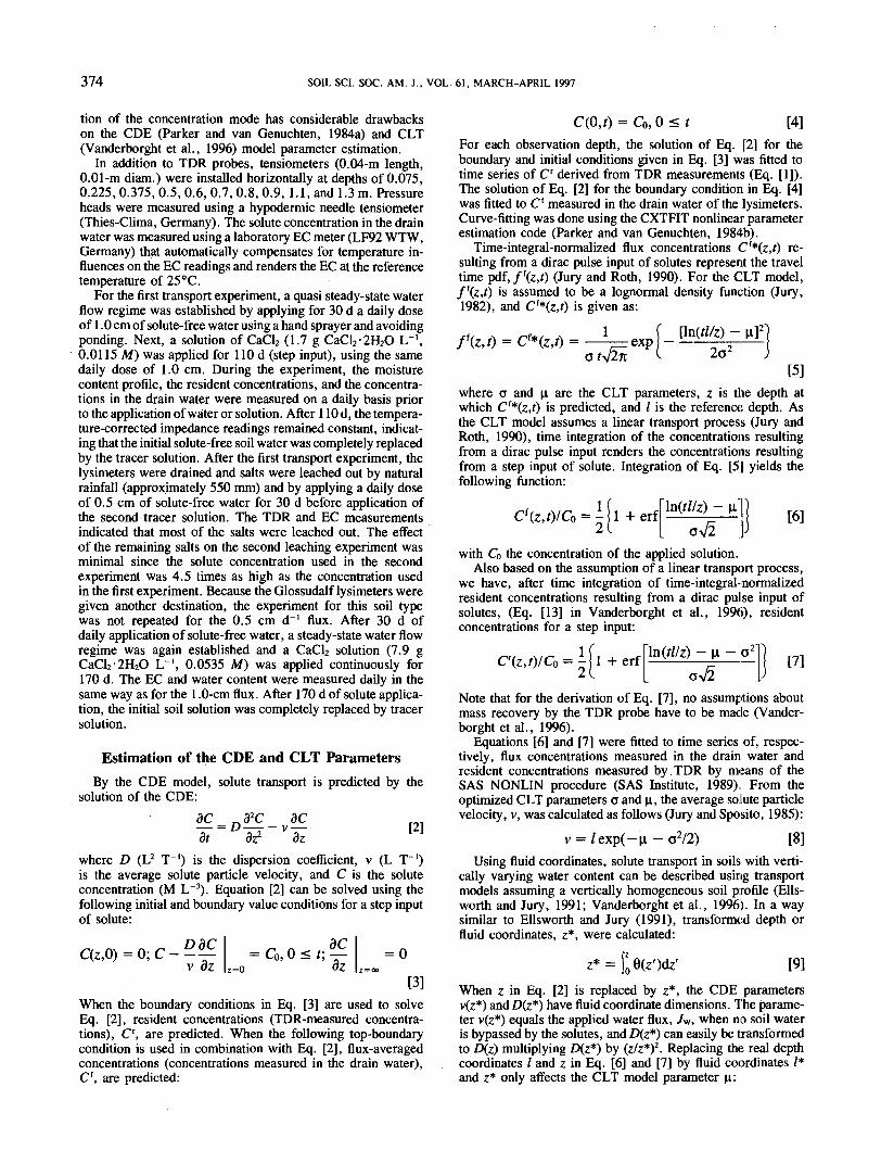
For the first transport experiment, a quasi steady-state waterflow regime was established by applying for 30 d a daily doseof 1.0 cm of solute-free water using a hand sprayer and avoidingponding. Next, a solution of CaCl2 (1.7 g CaCl2-2H2O LT',0.0115 A/) was applied for 110 d (step input), using the samedaily dose of 1.0 cm. During the experiment, the moisturecontent profile, the resident concentrations, and the concentra-tions in the drain water were measured on a daily basis priorto the application of water or solution. After 110 d, the tempera-ture-corrected impedance readings remained constant, indicat-ing that the initial solute-free soil water was completely replacedby the tracer solution. After the first transport experiment, thelysimeters were drained and salts were leached out by naturalrainfall (approximately 550 mm) and by applying a daily doseof 0.5 cm of solute-free water for 30 d before application ofthe second tracer solution. The TDR and EC measurementsindicated that most of the salts were leached out. The effectof the remaining salts on the second leaching experiment wasminimal since the solute concentration used in the secondexperiment was 4.5 times as high as the concentration usedin the first experiment. Because the Glossudalf lysimeters weregiven another destination, the experiment for this soil typewas not repeated for the 0.5 cm d"1 flux. After 30 d ofdaily application of solute-free water, a steady-state water flowregime was again established and a CaCl2 solution (7.9 gCaCl2-2H2O L~', 0.0535 Af) was applied continuously for170 d. The EC and water content were measured daily in thesame way as for the 1.0-cm flux. After 170 d of solute applica-tion, the initial soil solution was completely replaced by tracersolution.

Estimation of the CDE and CLT ParametersBy the CDE model, solute transport is predicted by the

solution of the CDE:dC nd2C dC— = D—— — v —dt dz2 dz [2]

where D (L2 T~') is the dispersion coefficient, v (L T"1)is the average solute particle velocity, and C is the soluteconcentration (M L~3). Equation [2] can be solved using thefollowing initial and boundary value conditions for a step inputof solute:

= C0,0<^z=0

= 0

[3]When the boundary conditions in Eq. [3] are used to solveEq. [2], resident concentrations (TDR-measured concentra-tions), C', are predicted. When the following top-boundarycondition is used in combination with Eq. [2], flux-averagedconcentrations (concentrations measured in the drain water),Cf, are predicted:

) = Co, O < t [4]For each observation depth, the solution of Eq. [2] for theboundary and initial conditions given in Eq. [3] was fitted totime series of Cr derived from TDR measurements (Eq. [1]).The solution of Eq. [2] for the boundary condition in Eq. [4]was fitted to C' measured in the drain water of the lysimeters.Curve-fitting was done using the CXTFIT nonlinear parameterestimation code (Parker and van Genuchten, 1984b).

Time-integral-normalized flux concentrations Cf*(z,f) re-sulting from a dirac pulse input of solutes represent the traveltime pdf,/f(z,0 (Jury and Roth, 1990). For the CLT model,f'(z,f) is assumed to be a lognormal density function (Jury,1982), and Cf*(z,0 is given as:

= Cf*(z,0 =1 exp [\n(tl/z) -

2o2

[5]where a and n are the CLT parameters, z is the depth atwhich Cf*(z,r) is predicted, and / is the reference depth. Asthe CLT model assumes a linear transport process (Jury andRoth, 1990), time integration of the concentrations resultingfrom a dirac pulse input renders the concentrations resultingfrom a step input of solute. Integration of Eq. [5] yields thefollowing function:

Cf (z, O/Co = j l + erf \n(tl/z) -[6]

with Co the concentration of the applied solution.Also based on the assumption of a linear transport process,

we have, after time integration of time-integral-normalizedresident concentrations resulting from a dirac pulse input ofsolutes, (Eq. [13] in Vanderborght et al., 1996), residentconcentrations for a step input:

0(z,t)IC0 = 1 [7]

Note that for the derivation of Eq. [7], no assumptions aboutmass recovery by the TDR probe have to be made (Vander-borght et al., 1996).

Equations [6] and [7] were fitted to time series of, respec-tively, flux concentrations measured in the drain water andresident concentrations measured by TDR by means of theSAS NONLIN procedure (SAS Institute, 1989). From theoptimized CLT parameters o and fi, the average solute particlevelocity, v, was calculated as follows (Jury and Sposito, 1985):

v = /exp(-n-o2/2) [8]Using fluid coordinates, solute transport in soils with verti-

cally varying water content can be described using transportmodels assuming a vertically homogeneous soil profile (Ells-worth and Jury, 1991; Vanderborght et al., 1996). In a waysimilar to Ellsworth and Jury (1991), transformed depth orfluid coordinates, z*, were calculated:

[9]When z in Eq. [2] is replaced by z*, the CDE parametersv(z*) andD(z*) have fluid coordinate dimensions. The parame-ter v(z*) equals the applied water flux, 7W, when no soil wateris bypassed by the solutes, and D(z*) can easily be transformedto D(z) multiplying D(z*) by (z/z*)2. Replacing the real depthcoordinates / and z in Eq. [6] and [7] by fluid coordinates /*and z* only affects the CLT model parameter \i:


[10]

However, |i(z*) does not have fluid coordinate dimensionssince for a vertically homogeneous water content profile,u(z) = n(z*). Analogous to the CDE model, v(z*) calculatedfrom the CLT model parameters (Eq. [8] with / and u,(z)replaced by /* and (i(z*), respectively) equals 7w when no soilwater is bypassed.

Because solute resident concentrations are only measuredin the sampling volume of the TDR probe, the measuredresident concentrations may be different from the averageresident concentration in the soil at the sampling depth. Analo-gous to the notation used by Vanderborght et al. (1996), weuse tildes (v, D, p., d) for parameters that are derived fromtime series of resident concentrations and that describe solutetransport in the TDR-sampled soil volume only.

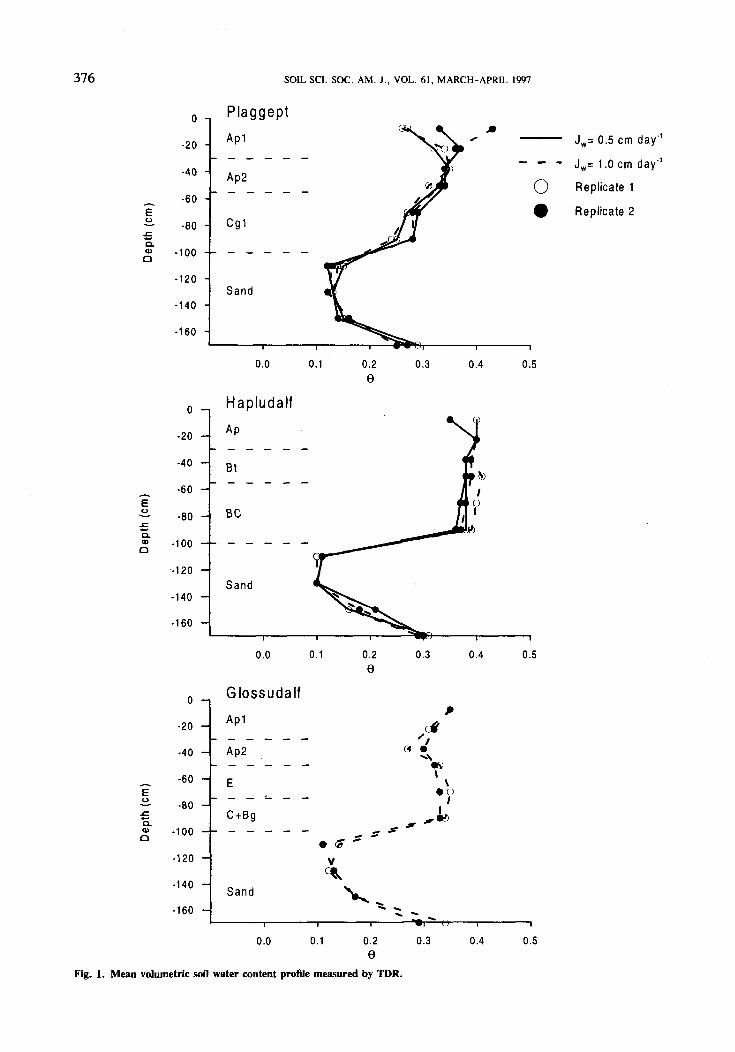
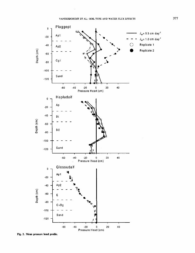
RESULTS AND DISCUSSIONIn Fig. 1 and 2, time-averaged soil water content

and pressure head profiles in the lysimeters are showntogether with the soil horizon boundaries. In general,soil water profiles show little variation with depth andwith water flux in the soil monoliths. Near the boundarybetween the soil monoliths and the repacked sand layerat a depth of 1 m, the water content in the repackedsand is considerably lower in comparison with the abovesoil horizon. Deeper in the sand layer, the water contentincreases again because of the saturated conditions atthe bottom of the sand column. At a given depth in thePlaggept soil, there are large variations in pressure head,which tended to decrease with decreasing water flow.Positive pressure heads in both the Plaggept and Haplu-dalf soils indicate the presence of less permeable layersimpeding the water flow. The increasing pressure headswith depth in the Hapludalf soils might be due to acompacted layer at the bottom impeding water flow andresulting from sampling disturbances. An alternative ex-planation might be that the tensiometer cups locallyimpede water flow in large pores, resulting in a buildupof water in those pores blocked by the tensiometer cups.The deeper the tensiometers are in the soil, the higherthe water column in the blocked pores.

Resident and Flux Concentrations for Three SoilTypes and Two Water Application Rates

Figures 3 to 5 show normalized resident concentrationsC/C0 as a function of time and depth. The horizontalbars in the graphs mark the observation depths. Timeseries of C/Co, observed at 10 depths in the lysimeters,were interpolated so that for the determination of C/C0(z,t), equal weight was given to observations C/Cb(z +Az,f) and C/C0(z,t + Af) for Af = Az0//w. In order tosimplify the interpolation, both 9 and Jw were assumedto be constant in both space and time for a given graphin Fig. 3, 4, and 5.

Superimposed on the plots is a "piston flow line",which represents the depth of the solute front with timefor the case of piston flow. Note that because (i) BTCswere skewed and (ii) resident concentrations are plotted,

the time at which the 0.5 iso-C/Cb line crosses a certaindepth is only a rough approximation of the average solutearrival time. A comparison between the piston flow lineand the 0.5 iso-C/Cb line gives an indication of the solutetransport heterogeneity.

From Fig. 3, it is apparent that in the Plaggept soil,solute transport is very heterogeneous. At some sites inthe soil monolith, the TDR measurement window seemsto be "bypassed" by the piston flow solute front sincethe piston flow line arrives much earlier than the 0.5iso-C/Co line, e.g. at the third and fourth observationdepths in Replicate 1 and at the second and third observa-tion depths in Replicate 2. At several other sites, the0.5 iso-C/Co line arrives earlier than the piston flow lineand even earlier than at shallower depths, e.g., at thefifth and sixth observation depths in Replicate 2. At thesesites, TDR probes seem to detect "preferential" solutetransport or solute transport faster than piston flow trans-port. It is also remarkable that bypass or preferentialsolute transport occurred at the same sites for the twowater fluxes. This indicates persistency of heterogeneoussolute flow in this soil type, which is analogous to thepersistent heterogeneity of water flow in water-repellentsandy soils reported by Ritsema et al. (1993).

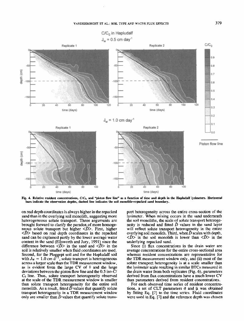
In the Hapludalf soil (Fig. 4), solute transport is fairlyhomogeneous for yw = 0.5 cm d"1. For Jw = 1.0 cmd~', the transport heterogeneity increased drastically.This heterogeneity is reflected in the long time betweenthe first arrival of solutes at a specific site and thecomplete replacement of the initial soil solution by theapplied solution at this site. Furthermore, the heterogene-ity for Jw = 1.0 cm d"1 is also apparent from observeddisparities between the 0.5 iso-C/Co line and the pistonflow line. Note the fast arrival of solutes in the repackedsand layer under Replicate 1, faster than in the overlyingsoil monolith, with solutes reaching a depth of 170 cmafter only 10 d of solute application. This indicatesthat fast solute transport must have bypassed the TDRmeasurement windows in the soil monolith, suggestingthat solutes are advected downward in macropores.

Solute transport in the Glossudalf soil (Fig. 5) wasvery homogeneous, compared with the two previouscases. The time between the first arrival of solutes andcomplete replacement by the applied solution at a specificdepth as well as deviations between the 0.5 iso-C/Coline and the piston flow line were small.

In Fig. 6, normalized flux concentrations are plottedvs. time. The flux concentrations were measured in thedrain water and can be considered to be representativefor the entire cross-sectional area of the lysimeter. Asthe differences between the BTCs from two replicatesfor the same water application rate are small, we mayconclude that the average solute transport process in thereplicate lysimeters is fairly similar.

CDE and CLT ParametersFor each observed time series of resident concentra-

tions, a set of CDE parameters D and v was obtainedfrom fitting the solution of Eq. [2] to the observed time


E

Q.010

0 -

-20 -

-40 -

-60 -

-80 -

-100 -

-120 -

-140 -

-160 -

PlaggeptAp1

Ap2

Cg1^

^Sand «

Ju^s

Q.O>Q

CLO>Q

Hapludalf

0.0 0.1

-20 -

-40 -

-60 -

-80 -

-100 -

-120 -

-140 -

-160 -

Ap

Bt_ _ _ _ _

BC

r^Sand V.

^^JN^^^^^_

0.2e

0.3 0.4

0.0 0.1 0.2 0.3e

Fig. 1. Mean volumetric soil water content profile measured by TDR.

0.4

Jw= 0.5 cm day'1

Jw= 1.0 cm day'1

Replicate 1

Replicate 2

0.0 0.1 0.2 0.3 0.4 0.59

0.5

0 -

-20 -

-40 -

-60 -

-80 -

•100 -

-120 -

-140 -

-160 -

C/- - - - - - '/

Ap2 (* »N

E_ _ _ _ _ _ •?

C + Bg i*)_ _ _ _ _ _ f f •*"

V

Sand >w^^^ ^

0.5


. — .

-H-•£_

0>Q

1"—Q.0)0

^

'Q.o>0

0 Plaggept

-20 -

-40 -

-60 -

-80 -

-100 -

-120 -

Glfl <L

Ap1 S^V- - — - - ^^vS,

Ap2 i Y

(g <3£ if

k^cCg1 NS\^- — — — — ,

Sand ' '1

» ^ -i-N

N ~"

y X >Ji

IT\

f'

\IV———— i ———— i ———— i — i — • -^ —— i ———— i ————-60 -40 -20 0 20 40

Pressure Head cm)

0 -

-20 -

-40 -

-60 -

-80 -

-100 -

-120 -

Hapludalf

Ap N\V

Bt v*. _ _ _ _

BC

*tfSand \

r?*a.rfAILjft®^

—————— 1 —————— 1 —————— 1 —— •BO —————— i —————— i ——————

-60 -40 -20 0 20 40Pressure Head (cm)

0 Glossudalf

-20 -

-40 -

-60 -

-80 -

-100 -

-120 -

Ap1

Ap2 *

E V

- - - - - *^

C + Bg ^

- - - - - ,1Sand Jt

I \

- Jw= 0.5 cm day'1

— - - Jw= 1.0 cm day'1

Replicate 1

Replicate 2

-60 -40 -20 O 20Pressure Head (cm)

40

Fig. 2. Mean pressure head profile.


C/C0 in PlaggeptJw = 0.5 cm day"1

Fig. 3. Relative resident concentrations, Cl Co, and "piston flow line" as a function of time and depth in the Plaggept lysimeters. Horizontal barsindicate the observation depths, dashed line indicates the soil monolith-repacked sand boundary.

series. Table 2 presents average values (< >) and CVsfor estimated COE parameters D and v together withthe dispersivity length, X = Div, combining parametervalues from all depths in both soil monoliths. Also shownare the average and CV of the estimated parameters forthe repacked sand underneath the soil monoliths and ofthe parameters fitted to flux concentrations in the drainwater. Because only two parameter values were obtainedfor the flux concentrations for each soil type, the standarddeviation used for the calculation of the CV was approxi-mated by the average deviation of the parameters fromtheir mean multiplied by a factor of 5/4 (Spiegel, 1992).The COE parameters are shown for real depth and fluidcoordinates, z* (Eq. [9]). Except for the Glossudalf andfor the Hapludalf for 7w = 0.5 cm d~', X values in thesoil monolith (8-16 cm) are considerably higher thanthe values reported for transport studies in repacked soilcolumns (Klotz et al, 1980; Wierenga and van Genuchten,1989; Khan and Jury, 1990; Vanclooster et al., 1993).All <Z)> values in the soil monoliths with real depthcoordinates (5.2-40.4 cm2 d"1) are considerably larger

than effective molecular diffusion coefficients in soils,which vary, depending on the soil type and water content,from 0.7 to <0.1 cn/d"1 (Beese and Wierenga, 1983).This indicates that even for the relatively low water fluxof 0.5 cm d~', the solute dispersion is mainly causedby hYdrodynamic dispersion. Note the large CVs of v, D,and Xin both the Plaggegt and Hapludalf soil monoliths.Similar large CVs for D and v have been reported inthe literature (Biggar and Nielsen, 1976; Bowman andRice, 1986^Mallantsetal., 1996a). Because the variabil-ity of v, D, and X using fluid coordinates was verysimilar to the variability of v, D, and X using real depthcoordinates (Table 2), the observed heterogeneity cannotbe attributed to vertical variations in soil water content.

In the repacked sand layers underneath the soil mono-liths, the CV of the CDE parameters is in general consid-erably less than in the soil monoliths. This illustratesthat solute transport in the repacked sand layer is morehomogeneous than in the overlying soil monolith. How-ever, merely looking at <£» in the repacked sand layerwould lead to the opposite conclusion since <D> based


C/C0 in HapludalfJw = 0.5 cm day"1

Fig. 4. Relative resident concentrations, Cl Co, and "piston flow line" as a function of time and depth in the Hapludalf lysimeters. Horizontalbars indicate the observation depths, dashed line indicates the soil monolith-repacked sand boundary.

on real depth coordinates is always higher in the repackedsand than in the overlying soil monolith, suggesting moreheterogeneous solute transport. Three arguments arebrought forward to clarify the paradox_of more homoge-neous solute transport but higher <D>. First, higher<D> based on real depth coordinates in the repackedsand can be explained partly by the lower average watercontent in the sand (Ellsworth and Jury, \99\)_ since thedifference between <D> in the sand and <Z>> in thesoil is relatively smaller when fluid coordinates are used.Second, for the Plaggept soil and for the Hapludalf soilwith Jw = 1.0 cm d~', solute transport is heterogeneousacross a larger scale than the TDK measurement window,as is evident from the large CV of v and the largedeviations between the piston flow line and the 0.5 iso-C/Co line. Thus, solute transport heterogeneity observedat the scale of the TDR measurement window is smallerthan solute transport heterogeneity for the entire soilmonolith. As a result, fitted D values that quantify solutetransport heterogeneity in a TDR measurement windowonly are smaller than D values that quantify solute trans-

port heterogeneity across the entire cross-section of thelysimeter. When mixing occurs in the sand underneaththe soil monoliths, the scale of solute transport heteroge-neity is reduced and fitted D values in the sand layerwill reflect solute transport heterogeneity in the entireoverlying soil monolith. Third, when D scales with depth,<D> in the soil monolith is lower than <D> in theunderlying repacked sand.

Since (i) flux concentrations in the drain water areaverage concentrations for the entire cross-sectional areawhereas resident concentrations are representative forthe TDR measurement window only, and (ii) most of thesolute transport heterogeneity is at a scale smaller thanthe lysimeter scale resulting in similar BTCs measured inthe drain water from both replicates (Fig. 6), parametersderived from flux concentrations have a much lower CVthan parameters derived from resident concentrations.

For each observed time series of resident concentra-tions, a set of CLT parameters a and p, was obtainedby fitting Eq. [7] to the time series. Fluid coordinateswere used in Eq. [7] and the reference depth was chosen


C/C0 in GlossudalfJw = 1.0 cm day"1

Piston flow lineFig. 5. Relative resident concentrations, C/C0, and "piston flow line" as a function of time and depth in the Glossudalf lysimeters. Horizontal

bars indicate the observation depths, dashed line indicates the soil monolith-repacked sand boundary.

/* = 20 cm. Average CLT parameters <d> and <fi>together with their CVs are given in Table 3, combiningparameter values from all depths in both soil monoliths.Also given is the average and CV of v (expressed influid coordinates), derived from d and p, (Eq. [S]).The average parameters and their CVs pertaining to therepacked sand underneath the soil monoliths and thedrain water are also shown in Table 3. A comparisonbetween <d> listed in Table 3 and parameter valuesreported in other studies is difficult, as <d> has beendetermined in relatively few studies (Jury and Scotter,1994). Furthermore, in most studies, <d> was derivedfrom the variability of v or from concentrations, bothmeasured across a larger scale than in this study (Juryet al., 1982; Jury, 1985; Butters and Jury, 1989; Mallantset al., 1996a).

The CV of d is considerably smaller than the CVof D except for the Glossudalf soil. From a pairwisecomparison of v derived from COE and CLT model fitsto time series of resident concentrations, it follows thatthe latter are significantly (at the 0.05 level) larger thanthe former. As was shown by Jury and Roth (1990,p. 56-57), when COE and CLT predictions of fluxconcentration match perfectly, CLT and COE predictionsof resident concentrations are different. As a direct conse-quence, when CLT and CDE model predictions of resi-dent concentrations match, predictions of the flux concen-trations are different, which explains the differences inv predicted by the two models.

In the repacked sand underneath the Glossudalf andfor /w = 0.5 cm d"1 underneath the Plaggept and Haplu-

dalf soils, <d> is lower than in the overlying soil mono-lith. This decrease of <d> indicates solute mixing inthe repacked sand. The value of <d> estimated fromflux concentration BTCs in the drain water is lower than<d> in the repacked sand layer under the Plaggept andHapludalf soil monoliths, which is another indication ofsolute mixing in the homogenous repacked sand. Thehigher <d> in the repacked sand layer underneath thePlaggept and Hapludalf soils for /w = 1.0 cm d"1 canbe explained by the scale of solute transport heterogeneityin the soil monoliths, which is larger than the TDRmeasurement window.

A comparison of v based on fluid coordinates with/w, can be used to detect possible bypass flow or anionexclusion (v > Jw), or to detect the effects of hysteresisand soil heterogeneity in combination with transient flow(v < 7W) (Russo et al., 1989). For the Glossudalf soil,<v> was larger (20% for the CDE and 25% for theCLT model) than 7W (significant at the 0.05 level), whichindicates some preferential flow or anion exclusion. Thecombined effect of bypass flow and anion exclusion onthe average solute velocity observed here is small com-pared with the bypass flow reported by Bowman andRice (1986) (v 60-70% larger than Jw) and by Dysonand White (1987) (v 50-200% larger than /w). In theHapludalf soil for /w = 0.5 cm d"1, <v> is larger (10%for the CDE and 20% for the CLT model) than 7W(significant at the 0.05 level), indicating bypass flow oranion exclusion. For /w = 1.0 cm d~', <v> is smaller(30% for the CDE and 10% for the CLT model) than

OO

VANDERBORGHT ET AL.: SOIL TYPE AND WATER FLUX EFFECTS

Plaggept (Jw = 0.5 cm day'1) Plaggept (Jw = 1.0 cm day"1)

381

1.0 -

0.8 --

0.6 --

0.4 -

0.2 -

0.0 -

w*0 1.0 — i

f 0.8 -f/ 0 0.6 -

t ^/ ° 0.4 -

£ 0.2 -Es

— - i — y i — [ — i — | — i — | — i — j 0.0 -

J^ 8

g

#8'

O

CW|OA

(P•

<?

P ' 1 ' I ' 1

40 80 120 160 200Days

40 80Days

120

Hapludalf (Jw = 0.5 cm day'1)

O

1.0 -

0.8 -

0.6 -

0.4 -

0.2 -

O.Oi

Hapludalf (Jw = 1.0 cm day")O

Days

/

0.8 -

o 0.6 -

0 0.4 --

0.2 -

I ' I ' I 0.0 -|-- • T • 1 —— • "I

O

«£%

Oy/'

jgrn"«•*

<p

120 160 200 0 40 80 12Days

Glossudalf (Jw = 1.0 cm day"1

O replicate 1

replicate 2

O

o.o

Fig. 6. Relative flux concentrations, C/C0, measured in the drain water from the lysimeters.

/w in the Hapludalf soil although this difference is not macropores are activated, which would result in moresignificant at the 0.05 level. This is contradictory to bypass flow. In the Plaggept soil, the differences betweenwhat we would expect. For a higher water flow, more <v> and Jw were not significant at the 0.05 level.

382 SOIL SCI. SOC. AM. ] . , VOL. 61, MARCH-APRIL 1997

Table 2. Estimated convective-dispersive model parameters.

Real depth coordinates

MonolithtSandtDrain water}





<v>

cm d"1

1.582.282.09

2.844.573.82

1.461.781.77

1.894.293.26

3.594.303.63

CV f

43270

48218

1183

40253

6102

<D>

cm2 d'1

18.024.821.4

33.8162.677.7

5.2010.689.43

40.37378.40223.80

6.4411.5420.30

CV D

%

1848230

96505

814010

1285218

34255

<)> CVX

cm %Plaggept, Jw

8.23 13910.01 6410.20 30

Plaggept, Jw

10.57 7840.23 8520.40 4

Hapludalf, Jw

3.41 735.99 385.34 13

Hapludalf, Jw

15.94 9482.54 3268.80 20

Glossudalf, Jw

1.78 292.66 205.61 7

<v>

cm d~'= 0.5 cmd- '

0.500.590.49

= 1.0 cmd- 1

0.931.220.93

= 0.5 cm d'1

0.560.550.50

= 1.0cm d-'0.731.350.93

= 1.0 cm d-'1.191.190.93

CV f%

44313

49243

1333

40221

771

Fluid coordinates

<D>

cm2 d-'

1.981.551.16

3.7611.564.64

0.771.030.75

5.9237.1118.08

0.700.881.34

CV D

1867224

9249

5

843511

1275021

33148

<X>

cm

2.742.502.38

3.5610.664.99

1.311.871.51

6.1126.2719.55

0.590.741.44

cvx

1415927

75799

743614

942922

29149

t Resident concentrations.} Flux concentrations.

Identification of the Solute Transport ConceptJury and Roth (1990) demonstrated that determining

whether the governing transport process is stochastic-convective (CLT model) or convective-dispersive (CDEmodel) requires BTCs observed at different depths in thesoil profile. The stochastic-convective and convective-dispersive transport process hypotheses were evaluatedby testing the depth dependency of the CLT and CDE

Table 3. Estimated convective lognormal transfer function modelparameters.

CV CT CV ji <v>% cm d"1

Plaggept, Jw = 0.5 cm d~'


0.4450.3470.318

482514

3.553.443.66

1591

0.5520.6250.488

Plaggept, Jw = 1.0 cm d~'

t Resident concentrations.} Flux concentrations.

CV v

53324





0.5770.5940.471

0.3740.2820.235

0.6910.8840.804

0.3230.1950.24

22 2.8613 2.434 2.97Hapludalf, Jw

21 1.5617 3.516 3.67Hapludalf, Jw

29 2.9410 2.0513 2.79

Glossudalf, Jw

43 2.7113 2.7784 3.038

17101

= 0.5 cm

1310

= 1.0 cm18141

= 1.0 cm520

1.0731.5020.922d-'0.5990.5760.4%d-'0.8891.7810.890d-1

1.2551.2220.932

49222

1531

45245

971

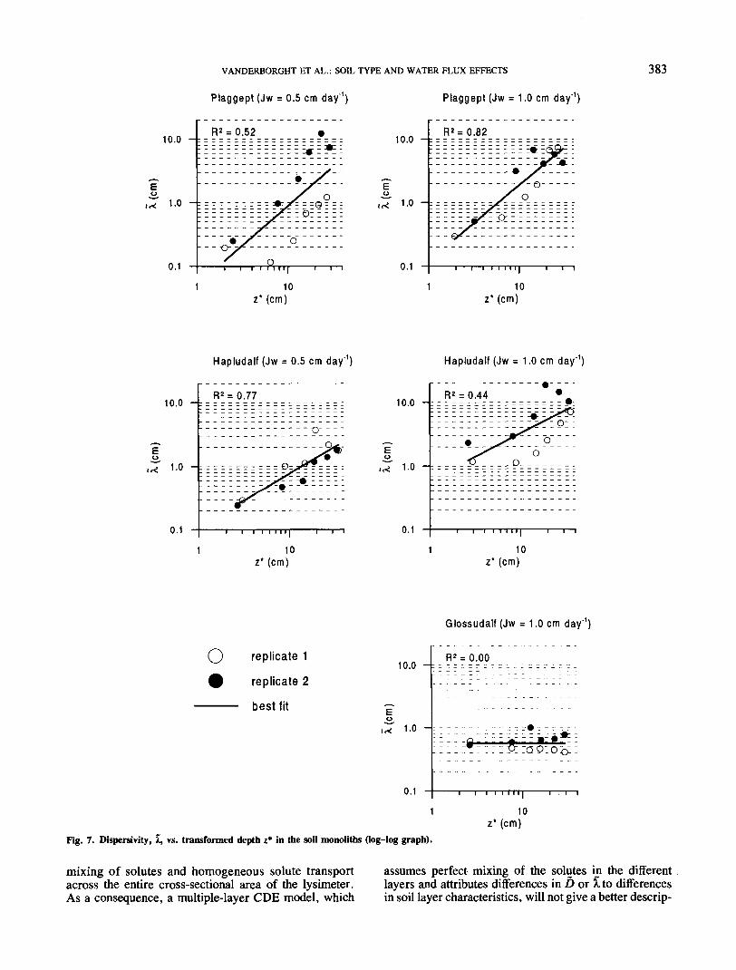
parameters obtained from fitting the model to BTCsobserved at different depths (Khan and Jury, 1990_; Van-derborght et al., 1996). When the dispersion, D, anddispersivity, X, remain constant with depth, title solutetransport is better modeled by a convective-dispersiveprocess, whereas a constant d parameter indicates astochastic-convective process. Furthermore, a constantD or Ximplies a decreasing d with depth [d2 ~ ln(l +1/z2)], whereas a constant d implies a linear increase ofD or X with depth. Estimated values for CDE parameterXand CLT parameter d are plotted vs. z* in Fig. 7 and8, respectively . For the X parameter, a logio transforma-tion was performed because the variability of A, betweenthe replicates increased with depth. After this transforma-tion, the variability of logio(X) remained constant withlogio(z*), making statistical inference about the relation-ship between logio(X) and logio(z*) meaningful. For theGlossudalf soil, X did not increase with depth, whereasfor the Hapludalf and Plaggept soils, X increased signifi-cantly (at the 0.05 level) with depth for both waterapplication rates. The CLT parameter d decreased withdepth in the Glossudalf soils, but remained fairly constantin the Hapludalf and Plaggept soils. Based on the behaviorof the CDE and CLT parameters with depth, solutetransport in the Glossudalf soil is better modeled asa convective-dispersive process, whereas a stochastic-convective process seems more appropriate in tine Haplu-dalf and Plaggept soils. An additional argument for thevalidity of the stochastic-convective transport hypothesisin both Hapludalf and Plaggept soils is the large variabil-ity of v based on fluid coordinates (Tables 2 and 3).This variability illustrates the heterogeneity of solutetransport in the lysimeter, which is contradictory tothe convective-dispersive transport hypothesis of perfect

VANDERBORGHT ET AL.: SOIL TYPE AND WATER FLUX EFFECTS

Plaggept (Jw = 0.5 cm day"1) Plaggept (Jw = 1.0 cm day'1)

10.0 -:

EU

1-0 -

0.1

R2 = 0.52

10z * ( cm)

10.0 -:

1.0 -:

0.1

R2 = 0.82

1 10z* (cm)

383

10.0 -:

EU

0.1

Hapludalf (Jw = 0.5 cm day"1)

R2 = 0.77

T ' ""I10

z* (cm)

10.0 -:

1.0 - :

0.1

Hapludalf (Jw = 1.0cm day"1)

R2 = 0.44

10z* (cm)

O replicate 1

replicate 2

best fit

10.0 -:

EO

,<< 1.0 H

0.1

Glossudalf (Jw = 1.0 cm day"1)

R2 = 0.00

Fig. 7. Dispersivity, X, vs. transformed depth z* in the soil monoliths (log-log graph).

10z* (cm)

mixing of solutes and homogeneous solute transport assumes perfect mixing of the solutes in the differentacross the entire cross-sectional area of the lysimeter. layers and attributes differences in D or Xto differencesAs a consequence, a multiple-layer CDE model, which in soil layer characteristics, will not give a better descrip-


Plaggept (Jw = 0.5 cm day Plaggept (Jw = 1.0 cm day'1)

1.0 -i

0.0

1.0 -

0.8 -

. 10 -• 0.4 -

0 O O

0 ° 0.2 -

1 —— ' —— 1 —— ' —— 1 —— ' —— 1 —— ' —— 1 °'° -| —— • —— 1 —— • —— 1 —— ' —— 1 —— ' —— i

*ooo ' ° ' ° .

) 10 20 30 40 0 10 20 30 40z* (cm) z * ( cm)

Hapludalf (Jw = 0.5 cm day"1) Hapludalf (Jw = 1.0 cm day''

1.0 -

0.8 -

0.6 -

0.4 -

0.2 -

0.0 -

(

1.0 -

0.8 -

0 °'6 ~10

« °' o . o

0.2 -

—— i | i | , ! , ) 0.0 -|— r-, , ,-- r | ,--,

•

o • • •

0 °o 0 o

) 10 20 30 40 0 10 20 30 40z* (cm) z * ( c m )

Glossudalf (Jw = 1 .0 cm day"

1.0 -O replicate 1

0.8 -9 replicate 2

0.6 -10

0.4 -

0.2 -

0.0 -

(

8

8 •° * 8 .

1 I ' 1 ' I) 10 20 30

z* (cm)Fig. 8. Convective lognormal transfer function model parameter a vs. transformed depth z* in the soil monoliths.

tion of the transport process. Furthermore, given thelarge differences between the CDE or CLT parameterestimates in the two replicates at a specific observationdepth, the effect of soil layering on the solute transportprocess could not be investigated in this study. A rel-

atively constant d (Plaggept and Hapludalf soils) orX (Glossudalf soil) with depth indicates that solute trans-port in the layered soil profiles may be described byonly one set of parameters, as in a vertically homoge-neous profile.


Table 4. Coefficient of variation of the soil water content in ahorizontal plane, CV 6, and of the solute particle velocity withfluid coordinates, CV v.

eve cv

Plaggept, Jw = 0.5 cm d'1

Plaggept, Jw = 1.0 cm d"1

Hapludalf, Jw = 0.5 cm d~'Hapludalf, Jw = 1.0 cm d'1

Glossudalf, Jw = 1.0 cm d"1

534915459

Estimation of the Average Solute Transportin a Heterogeneous Soil

As was pointed out above, the variability of v couldnot be explained by vertical variations in soil watercontent. Furthermore, we calculated the CV of the localsoil water content, CV 0, in a horizontal plane. Becauseonly two observations were available per depth, weassumed that CV 0 was constant with depth. We furtherassumed that 0 was lognormally distributed such thatCV 0 can be calculated from

CV 0 = Vexp(oie) - 1 [11]where o?ne is the variance of ln(0). The value of o?n8 wascalculated as follows:

S [ln(0),v -oie = JL

N[12]

where ln(0), j is the natural logarithm of soil water contentmeasured at the /th observation depth in they'th replicate,<ln(0)/> is the average natural logarithm of the soil watercontent at the ith observation depth, and N is the numberof observation depths. If the heterogeneity of the soluteparticle velocity v was due to local variations in soilmoisture content, then CV v should resemble CV 0. InTable 4, values for CV 0 (Eq. [11]) and CV v are listed.Values for CV 0 are fairly similar for all soil types andthe two water application rates and are in agreementwith typical values of CV for porosity measurementsreported by Jury (1985). The homogeneous convective-dispersive solute transport in the Glossudalf soil wascharacterized by a CV v that was only 5% larger thanCV 0. In the Plaggept and Hapludalf soils, CV v wasconsiderably larger than CV 9, indicating that the hetero-geneity in v cannot be explained by local differences in0. The heterogeneity in v also cannot be attributed to anonuniform solute and water application. Since solutionwas manually applied daily, there was no consistencyin the spatial pattern of possible nonuniform solute appli-cation so that nonuniformity at one day was compensatedby nonuniformity at other days. Jury and Scotter (1994)discussed two mechanisms that could enhance the vari-ability of v. First, when the volumetric water contentcan be split up into two subvolumes, a mobile zone inwhich the solutes are conducted downward relativelyfast and an immobile zone that does not contribute todownward solute transport, the variability of the mobilewater volume may exceed the variability of the totalwater volume considerably. For instance, Mallants etal. (1996a) obtained a CV of 150% for the ratio of themobile water content to the total soil water content ina macroporous sandy loam soil (Udifluvent). In case there

is lateral solute exchange between mobile and immobilezones, the average solute particle velocity is determinedby the ratio of the water flux to the total volumetricwater content (Valocchi, 1985). As a consequence, whenthe water flux is uniform throughout the entire cross-section, the heterogeneity of v is only determined bylateral variability of the total water content and shouldbe small. Thus, assuming uniform water flux and mobileand immobile zones, the large heterogeneity of v derivedfrom COE or CLT model fits can be explained merely bya lack-of-fit between model predictions and observations.Because the mobile-immobile model (van Genuchtenand Wierenga, 1976) assuming homogeneous water flow(i) did not give better fits than the CDE or CLT models,and (ii) rendered extreme parameter values that couldhardly be interpreted physically and that were very uncer-tain (results not shown), we concluded that (i) the assump-tion of homogeneous water flow was not valid and (ii)the variability of v cannot be explained by mobile andimmobile zones. Second, the variability of v can alsobe enhanced by lateral redistribution flow near the inletsurface resulting in larger water flow heterogeneity inthe soil than at the inlet surface. Experimental evidenceof the existence and importance of this process at thelysimeter scale in different soil types is reported in theliterature (Kung, 1990; Ritsema et al., 1993; Poletikaand Jury, 1994; Quisenberry et al., 1994).

In order to account for the effect of heterogeneityof water flow on solute transport in the Plaggept andHapludalf soils, we used the following transport concept.Because solute transport was stochastic-convective inthese soils, we assumed that solutes were transported indifferent stream tubes that originated close to the soilsurface because of redistribution flow. Furthermore, itwas assumed that solute transport in each set of streamtubes sampled by a TDR probe can be described as afunction of the cumulative drainage, / = Jv/t, usingthe CLT-model cumulative drainage pdf fi (z,I) withdeterministic parameters o/ and \ii, which is identical toEq. [5] with t, ]i, and o in Eq. [5] replaced by /, n/,and o/, respectively. Note that parameters o/ of thecumulative drainage pdf,//(z,/), and a of the travel timepdf in the sampled set of stream tubes are equal and canbe interchanged. The assumption of one deterministico/, which can be used to describe solute transport ineach sampled set of stream tubes, is justified from thelow CV of o. Since the variability of 9 in a horizontalplane was low, 0(z) was assumed to be deterministic sothat /w in a sampled set of stream tubes is equal to vexpressed in fluid coordinates. Thus high values of vimply a high /w and, as a direct consequence, a highsolute flux or mass recovery in the sampled set of streamtubes. The assumption of deterministic 0(z) and o/impliesa deterministic (i/ [\ii = ln(/*) — o/2/2]. In fact, thestream tube model considered here is analogous to solutetransport for spatially variable water application withthe only difference that the variability of the water flowhere is due to redistribution flow in the top layer of thesoil. The travel time pdf describing solute transport inthe entire population of stream tubes, ff(z,t), is thengiven as (Jury and Roth, 1990, p.75):


f(z,t) = d/w [13] is Proportional to /w or v

where .//wC/w) is the pdf of Jw and ./}w(./w)d./w is theprobability that solutes are transported in a set of streamtubes with a flux between 7W and 7W + d/w. When weassume that .//wG/w) is a lognormal pdf with parametersUvw and Oy* that are constant with z*, it follows fromEq. [13] that/f(z,f) is also a lognormal travel time pdf(Eq. [5]) with parameters

M, = UY - uvw [14a]o2 = o? + a}w [14b]

Since the solute mass in a sampled set of stream tubes

/v(v)dv [15]

with /o(v)dv the probability of sampling a set of streamtubes with a velocity (flux) between v and v + dv. FromEq. [15] follows that if/}w(Jw) is lognormal, /(.(v) is alsolognormal so that Eq. [14] can be written as a functionof <v> and o?n(io, the variance of /v(v), as

\i = - - o?n(i,) - - <6>2

02 = + <6>2

[16a]

[16b]

Plaggept (Jw = 0.5 cm day"1) Plaggept (Jw = 1.0 cm day"1)

0.04 -i 0.08 -i

OO

0.02 -

0.00

100

0.04 -i

0.02 -O

0.00

Hapludalf (Jw = 0.5 cm day'1)

O 40 80 120 160Days

OOO

0.06 -i

0.04 -

0.02 -

0.00

Hapludalf (Jw = 1.0 cm day"1)

i ' I r IO 20 40 60 80 100

Days

C' Eq.(17)

———— f' Eq.(5)and Eq.(16)

~~~~ f' Eq. (5)and Eq. (16) with a|n(5) = OFig. 9. Effect of observed velocity heterogeneity in Plaggept and Hapludalf soil monoliths on predicted flux concentrations representative for the

entire cross-sectional area of the lysimeter.


where o/ was replaced by <d>. Since Oyw is assumedto be constant with z*, ofnw is constant with z* and canbe calculated from v obtained at different depths. InTable 5, o, o2,, , and <d>, which represent, respec-tively, solute transport heterogeneity in the entire popula-tion of stream tubes, heterogeneity between differentsampled sets of stream tubes, and heterogeneity in asampled set of stream tubes, are listed. Figure 9 showspredicted average normalized flux concentration at adepth of z* = 20 cm obtained from ff(z,f) using nand o2 calculated from Eq. [16], with and without thesimplifying assumption, o?n(o) = 0. Also shown are thenormalized flux concentrations, Cf(z,t), predicted with-out the assumption of a lognormal pdf for /w and adeterministic o/:

[17]N

where Ji(z,t) is the CLT model travel time pdf calibratedfor the set of stream tubes sampled by the j'th TDRprobe, (v,7<v>) is a weighting factor giving more weightto concentrations measured in a set of stream tubes witha high water flux, and N is the number of TDR probes(12 for each soil type and water application rate). Theaverage normalized flux concentrations, Cf(z,f), pre-dicted by means of Eq. [17] coincided well with thosepredicted by Eq. [5] in combination with Eq. [16], indi-cating that the assumptions of deterministic d and alognormal pdf of v were reasonably well met, exceptfor the Plaggept soil with 7y = 0.5 cm d"1. For thisparticular case, the BTG of Cf(z,t) had a bimodal shape.This bimodal distribution could reflect an underlyingbimodal distribution of v or could result from averaginga limited number of v observations. Except for the Haplu-dalf soil with water application rate of 0.5 cm d~',neglecting oin^ resulted in considerable underestimationof a (for oin(j) = O, o = <d> (Eq. [16b]), which inturn resulted in less skewed BTCs with a later arrivalof the peak concentrations (Fig. 9). Therefore, we con-cluded that the observed solute flow heterogeneity be-tween different sampled sets of stream tubes in the Plag-gept soil for both water application rates and for theHapludalf soil for a water application rate of 1.0 cm d~'considerably influenced solute transport.

In order to test the applicability of the assumptionsmade for the identification of solute transport parametersrepresentative for the entire cross-sectional area of thelysimeter, |i and o2, a larger measurement window ofthe TDR probes is required or flux concentrations shouldbe monitored at the bottom of the soil monolith. In cased is about 0.5 and the CV of v is <20%, o2

n(c) is negliablecompared with d2, and d can be used to describe solutetransport in the entire set of stream tubes (see Jury [1982]and Jury and Roth [1990, p. 76]). To reduce the CV ofv of 50% observed in this study by a factor 2.5, thenumber of sampled stream tubes or the area for whichthe solute transport is measured and averaged shouldincrease by a factor of 6 (2.52). This means that six

TDR probes of the same geometry should be insertedat the same observation depth.

Effect of Water Application Rate on SoluteTransport Parameters

From a pairwise comparison of d values, we concludedthat d increased significantly (at the 0.05 level) with /win both Hapludalf and Plaggept soils. The value of <d>(Table 3) increased with /w from 0.45 to 0.58 in thePlaggept soil and from 0.37 to 0.69 in the Hapludalfsoil. Based on 95% confidence intervals of a2

n(v), derivedusing the %2 distribution (Spiegel, 1992), we concludedthat in the Plaggept soil, a\n(f) did not change significantly,whereas, in the Hapludalf soil, it increased significantly(at the 0.05 level) with 7W from 0.15 to 0.43 (Table 5).We thus conclude that o2[<d>2 + o2n(v>] increased withJw in both Plaggept and Hapludalf soils and that thisincrease was larger in the Hapludalf soil. This conclusionis further affirmed from the increase of solute spreadingwith Jw in the flux concentration BTG measured in thedrain water (Fig. 6, Table 3). Since o2 depends on /w,both Plaggept and Hapludalf soils can be consideredClass II soils in which solute transport is rate dependent(Dyson and White, 1989). The increase of o2 with /wis in agreement with the linear relation between o2 andJw reported by Dyson and White (1987) for solute trans-port in a slowly permeable clay soil that cracks deeplyin dry seasons (vertic Cambisol).

An increase of d and o?n(v> with water flux indicatesthat the flow regime changes and that the increase ofwater flux probably leads to the addition of new streamtubes that had remained dry previously so that waterflow and solute transport become more heterogeneous.For the strongly structured Hapludalf soil, an increaseof Jw probably resulted in fast solute transport in newlyfilled macropores or large pores between structural ele-ments. An increase of /w in the structureless sandyPlaggept soil probably resulted in the formation of newstream tubes in the soil matrix. As the solute particlevelocity in the macropores is much larger than in thesoil matrix, increasing the water flow in structured soils,and as a consequence in the macropores, results in largerdifferences in solute particle velocity than in the casewhere water flow increases only in the soil matrix. Thismay explain the considerably larger increase of o2 with/w in the structured Hapludalf soil compared with thestructureless Plaggept soil. A larger increase of the solutedispersion with Jw in structured (heterogeneous, undis-turbed) soils compared with structureless (homogeneous,disturbed) has also been reported by Beese and Wierenga(1983) and by Khan and Jury (1990).

Table 5. Values of a, <TU,W, and a in both Plaggept and Hapludalfsoils.

0 O,*,-, <d>



Hapludalf, Jw = 0.5 cm d~'Hapludalf, Jw = l.Ocmd-'

0.6270.7560.4040.813

0.4420.4880.1520.428

0.4450.5770.3740.691


SUMMARY AND CONCLUSIONSBased on an inert tracer experiment in three different

soil types using two different water application rates,the following conclusions were drawn.

1. Solute transport at the lysimeter scale in soils exhib-iting heterogeneous water flow (Plaggept andHapludalf) was better modeled as a stochastic-convective transport process (CLT model). Bycomparison, the convective-dispersive transportconcept appeared more appropriate for the morehomogeneous solute transport in the Glossudalfsoil. This conclusion was based on the behaviorof CDE and CLT parameters, which were fittedto time series of resident concentrations measuredby TDR probes with depth. In the Plaggept andHapludalf soils, X increased significantly withdepth, whereas d remained fairly constant. In theGlossudalf soil, X remained constant whereas adecreased with depth. Because the model parame-ters (k for the Glossudalf soil and 6 for the Plaggeptand Hapludalf soils) did not vary consistently withdepth, no effect of soil layers on solute transportwas seen in this experiment.

2. In both Hapludalf and Plaggept soils, the waterflow and solute transport were heterogeneous at ascale larger than the TDR measurement window,resulting in a large variability of v. The effect ofthe variability of v on transport across the entiresurface of the lysimeter was estimated using astream tube model and was shown to be important.In order to obtain better information on the variabil-ity of v and of the solute transport, we suggest theuse of multiple TDR probes at the same observationdepth. This is of particular interest for investigationof ofn(f>) and solute transport across soil layers.

3. Since an increase of application rate resulted inboth Plaggept and Hapludalf soils in larger solutetransport heterogeneity, solute transport in bothsoil types was rate dependent. In the Hapludalf soil,this increase was more pronounced, presumablybecause of the increased water and solute flow inmacropores or large voids between the structuralelements, whereas in the Plaggept soil, the increaseof water flow probably resulted in the formationof new flow paths in the soil matrix. Based on <v>determined in the soil monoliths, we concludedthat neither considerable bypass flow nor increaseof bypass flow with increasing application rate wereobserved in either soil type. Because the top bound-ary condition or the water flux can significantlyinfluence the values of the solute transport parame-ters, the water flux used for determination of param-eters should resemble the flux prevailing undernatural conditions.

ACKNOWLEDGMENTSWe would like to thank the Belgian National Fund for

Scientific Research (N.F.W.O.) and the Belgian Institute forthe Encouragement of Research in Industry and Agriculturefor their financial support. The corresponding author is a

research assistant of the Belgian National Fund for ScientificResearch (N.F.W.O.). Technical assistance in the experimentalsetup by P. Janssens, F. Serneels, and W. Smets is highlyappreciated.

effects of soil type and water flux on solute transport

Documents