effects of loop detector installation on the portland ... · research report . agreement t2695,...
TRANSCRIPT

August 2010Gudmundur A. Bodvarsson
Stephen T. MuenchWA-RD 744.5
Office of Research & Library Services
WSDOT Research Report
Effects of Loop Detector Installationon the Portland Cement Concrete Pavement Lifespan: Case Study on I-5


Research Report Agreement T2695, Task 88
PCCP Best Practices
Effects of Loop Detector Installation on the Portland Cement Concrete Pavement Lifespan: Case Study on I-5
by
Gudmundur A. Bodvarsson Stephen T. Muench Graduate Assistant Assistant Professor
Department of Civil and Environmental Engineering University of Washington, Box 352700
Seattle, Washington 98195
Washington State Transportation Center (TRAC) University of Washington, Box 354802
1107NE 45th Street, Suite 535 Seattle, Washington 98105-4631
Prepared for Washington State Department of Transportation
Paula J. Hammond, Secretary
and in cooperation with U.S. Department of Transportation
Federal Highway Administration
August 2010

1. REPORT NO.
WA-RD 744.5
2. GOVERNMENT ACCESSION NO. 3. RECIPIENT’S CATALOG NO.
4. TITLE AND SUBTITLE
EFFECTS OF LOOP DETECTOR INSTALLATION ON THE PORTLAND CEMENT CONCRETE PAVEMENT LIFESPAN: CASE STUDY ON I-5
5. REPORT DATE
August 2010 6. PERFORMING ORGANIZATION
CODE
7. AUTHORS
Gudmundur A. Bodvarsson and Stephen T. Muench
8. PERFORMING ORGANIZATION
CODE
9. PERFORMING ORGANIZATION NAME AND ADDRESS
Washington State Transportation Center University of Washington, Box 354802 University District Building, 1107 NE 45th Street, Suite 535 Seattle, Washington 98105
10. WORK UNIT NO.
11. CONTRACT OR GRANT NUMBER
T2695-88
12. SPONSORING AGENCY NAME AND ADDRESS
Research Office Washington State Department of Transportation Transportation Building, MS 47372 Olympia, Washington 98504-7372 Project Manager: Kim Willoughby, 360-705-7978
13. TYPE OF REPORT AND PERIOD
COVERED
Research Report 14. SPONSORING AGENCY CODE
15. SUPPLIMENTARY NOTES
16. ABSTRACT
The installation of loop detectors in portland cement concrete pavement (PCCP) may shorten affected panel life, thus prematurely worsening the condition of the overall pavement. This study focuses on the performance of those loop embedded panels (LEP) by analyzing pavement data collected by WSDOT, and comparing it to the overall pavement performance on I-5 in King County. The results were divided by non-rehabilitated, diamond ground and dowel bar retrofit and diamond ground PCCP, as was done in the reference paper, to facilitate comparison. Overall, LEP perform worse – regarding panel cracking – in comparison to loop free panels (LFP), except on the small section of I-5 that has been Dowel Bar Retrofitted and Diamond grinded. For the non-rehabilitated PCCP, the difference between LEP and LFP with 1 crack is less than 1% but more than twice as many LEP have what is considered “failed” panels (2 or more cracks) than LFP. This might indicate that the loop installation affects more the severity of panel cracking than being the cause for it. Using these results and assuming panel replacement of the cost of $20,000 each, the cost of loop installation to the pavement was found to be $560 each. Traffic simulation was done for a section of I-5 to calculate delay due to lane closures, which loop detector installation constitutes. The user cost associated with the delay is a substantial part of the overall cost of loop installation, 40 – 60 percent depending on the number of affected lanes on the freeway. If user costs are accounted for, the overall cost of video and loop detection systems can be comparable. 17. KEY WORDS
Portland cement concrete pavement, loop detectors, pavement life, pavement performance, life cycle cost analysis
18. DISTRIBUTION STATEMENT
19. SECURITY CLASSIF. (of this report) 20. SECURITY CLASSIF. (of this page) 21. NO. OF
PAGES
22. PRICE

Table of Contents
1 Introduction ................................................................................................................. 1 1.1 Research Objective ............................................................................................. 2 1.2 Organization ........................................................................................................ 3
2 Background and Literature Review ............................................................................ 4 2.1 PCC pavement general characteristics ................................................................ 4 2.2 When should panels be replaced or reconstructed? ............................................ 4 2.3 Panel Replacement .............................................................................................. 5 2.4 Linear Cracking in PCC Pavement ..................................................................... 6 2.5 The VISSIM Simulation Program ...................................................................... 8 2.6 Inductive Loop Detectors .................................................................................... 8 2.7 Video Detectors ................................................................................................ 13 2.8 Life Cycle Cost Analysis .................................................................................. 16
3 Study Corridor and Data ........................................................................................... 16 3.1 Study Corridor .................................................................................................. 16 3.2 Field Data – Pavement Cracking ...................................................................... 23 3.3 Field Data – Traffic ........................................................................................... 27
4 Methods..................................................................................................................... 33 4.1 Pavement Distress Data Handling .................................................................... 33 4.2 Statistical Analysis ............................................................................................ 35 4.3 Traffic Data Handling ....................................................................................... 36 4.4 Traffic Simulation ............................................................................................. 36 4.5 Delay Time and Cost from Simulation ............................................................. 38
5 Data Analysis and Findings ...................................................................................... 42 5.1 Comparison – Cracked Panels with and without loops .................................... 43 5.2 Comparison – by sections ................................................................................. 47 5.3 Results – by type of loop .................................................................................. 50 5.4 Results – by lane ............................................................................................... 52 5.5 Results – by direction........................................................................................ 55 5.6 Cost – Inductive Loop Detectors and Video Detectors .................................... 57
6 Conclusions and Recommendations ......................................................................... 63 6.1 Conclusions ....................................................................................................... 63 6.2 Recommendations ............................................................................................. 65
References ......................................................................................................................... 67

List of Figures Figure 1. Typical crack formations (from Voigt 2002). ..................................................... 7Figure 2. Small loop shapes (from USDOT 2006). ............................................................ 9Figure 3. Inductive loop installation (from USDOT 2006). ............................................. 10Figure 4. Video detection from a side-mounted camera (USDOT 2006). ........................ 14Figure 5. Rehabilitation of PCC pavement on I-5 in King County as of 2004 ................. 20Figure 6. Types of loops: circle, rectangular with soft corners, rectangular with sharp corners and loop combo. ................................................................................................... 21Figure 7. Pavement distress data collection van (Pathway 2008). .................................... 23Figure 8. Pavement images displayed in Pathview II sofwware. ..................................... 25Figure 9. A whole concrete loop embedded panel ssembled from 8 separate images. .... 26Figure 10. Enlarged image of bottom left corner of Figure 8. .......................................... 27Figure 11. Loop detectors used in the simulation corridor. .............................................. 29Figure 12. Example of analyzed panels: cracks that were not counted. No cracks were counted for either of these panels. .................................................................................... 34Figure 13. Example of analyzed panels: cracks that were counted. One crack for each of these panels was counted as annotated by the arrows. ...................................................... 34Figure 14. Example of analyzed panels: patched panel. Four cracks were counted for this panel as annotated by the arrows. ..................................................................................... 35Figure 15. Snap shot of a simulation run. ......................................................................... 38Figure 16. Average cracking for non-rehabilitated PCC pavement. ................................. 44Figure 17. Average cracking for diamond ground PCC pavement. .................................. 45Figure 18. Average cracking for DBR PCC pavement. .................................................... 47Figure 19. Comparing LEPs and LFPs by section. ........................................................... 50Figure 20. Number of cracks in LEPs by type of loop detector. ...................................... 51Figure 21. Percentage of cracked LEPs by lane and rehabilitation type. ......................... 53Figure 22. Number of cracks by lane. ............................................................................... 55Figure 23. Cracked LEPs by lane and direction. .............................................................. 56

List of Tables Table 1. Strengths and Weaknesses of Inductive Loop Detectors (USDOT 2006) .......... 12Table 2. Strengths and Weaknesses of Video Detection (USDOT 2006). ....................... 15Table 3. Pavement Structure by Section from WSPMS (from Hansen et al. 2009). ........ 18Table 4. Example of single loop data output from TDAD ............................................... 31Table 5. Example of dual loop data output from TDAD .................................................. 31Table 6. Example of compiled data file for delay calculations ......................................... 39Table 7. Recommended Dollar Values per Vehicle Hour ................................................ 42Table 8. Average Cracking for Non-Rehabilitated PCC Pavement. ................................. 43Table 9. Average Cracking for Diamond Ground PCC Pavement ................................... 45Table 10. Average Cracking for DBR PCC Pavement. .................................................... 46Table 11. Comparing LEPs and LFPs by Section ............................................................. 49Table 12. Number of Cracks in LEPs by Type of Loop Detector .................................... 51Table 13. Percentage of Cracked LEPs by Lane and Rehabilitation Type. ...................... 52Table 14. Percent Truck Traffic by Lane .......................................................................... 54Table 15. Number of Cracks by Lane ............................................................................... 54Table 16. Cracked LEPs by Lane and Direction ............................................................... 56Table 17. Percentage of I-5 where LFPs are Cracked in Excess of 10% (from Hansen et al. 2007) ............................................................................................................................ 57Table 18. Calculations Increased Pavement Costs due to Loop Installations ................... 58Table 19. Lane Closure Results for 4 Lanes ..................................................................... 59Table 20. Lane Closure Results for 5 Lanes ..................................................................... 59Table 21. User Cost for 4 Lane Freeway due to Loop Installations ................................. 60Table 22. User Cost for 5 Lane Freeway due to Loop Installations ................................. 61Table 23. The Cost of Installing Loop Detectors and Video Detectors ............................ 62

Disclaimer The contents of this report reflect the views of the authors, who are responsible for the
facts and the accuracy of the data presented herein. The contents do not necessarily
reflect the official views or policies of the Washington State Department of
Transportation or the Federal Highway Administration. This report does not constitute a
standard, specification, or regulation.

1
1 Introduction The Portland cement concrete pavement (PCCP) on Interstate 5 was originally designed
to last 20 years. Whether it is the mild climate of western Washington or the quality of
aggregates used in the PCCP, the Portland cement concrete pavement in King County
has now been in service for more than twice its design life, or over 40 years. But with
average daily traffic of over 280,000, including 12,000 trucks and 50,000 daily transit
trips, the pavement is deteriorating fast (Parametrix 2008). Panel cracking, corner
breaking, faulting, patching and spalling are example of types of distress in the PCCP of
I-5. Field study has concluded that the average increase in cracking on I-5 is about 6
percent per year, which indicates that the increase in cracking after 5 years will be at
least 30 percent and at least 60 percent in 10 years. This would mean increasing number
of multiple cracked panels and therefore increased need for complete slab replacement
(Hansen et al. 2007).
There are over 800 loop detectors in the King County part of I-5, Milepost (MP)
139.9 – 177.7. The detectors measure occupancy and count the vehicles (and speed) as
they drive over them. They give valuable data about traffic which can be used for many
things, such as traffic forecasting, controlling traffic, online information about traffic and
much more. The loop detectors are considered rather reliable and a cheap option to get
this traffic data, but when they fail they are troublesome to repair, especially on a high
volume interstate like I-5 because of the required lane closures.
There is a concern that the actual means of installation of loop detectors (sawcut
into the concrete) may cause structural damage to those PCC pavement panels with

2
installed loop detectors. If this is the case, such structural damage would have to be
included in the lifecycle cost of loop detectors and could cause the overall cost of loop
detectors to rise dramatically perhaps making them less favorable traffic detection
option. In addition, if the traffic impact during installation and maintenance of loop
detectors are also taken into account the overall cost would likely rise further. Overall,
inclusion of PCC pavement performance effects and traffic user costs may provide a
better understanding of the true cost of loop detectors.
1.1 Research Objective This study attempts to determine whether or not loop detector installation methods
significantly affect long-term pavement performance. The area chosen for this study is
Interstate 5 (I-5) in King County. It contains over 800 loop embedded PCC pavement
panels. These loops may or may not be working and were installed using different
methods at various times over the pavement’s lifetime. This study will assess the
condition of these loop embedded panels (LEP) and compare them to the overall
pavement condition in the same area as reported in Hansen et al. (2007).
This will help better assess the true cost of inductive loop detectors (ILD) used to
obtain traffic data. In general, the ILD is thought of as an accurate low-cost means to
collect traffic data. However, if the real cost is higher than thought before because of
added pavement distress, such general assumptions may not hold true. Additionally, if
user delay costs during installation and maintenance of ILDs are accounted for then a
more accurate life cycle cost for ILDs can be reported.

3
1.2 Organization This report consists of six chapters:
• Chapter 2: an introduction to the basic concepts and tools used in this study
• Chapter 3: description of the study corridor and field data collected
• Chapter 4: research methods and data handling
• Chapter 5: data analysis and study findings
• Chapter 6: conclusions and recommendations

4
2 Background and Literature Review
In this chapter general information is provided on the principal concepts talked
about later in the paper, such as the concrete pavement and the rehabilitation techniques
that have been used in the study corridor, how and why the cracks come about and basic
information about the simulation program VISSIM which was used for calculations.
Detectors, both inductive loops and video detectors, are another part of the chapter, how
they work and the installation process. In the end of the chapter there is a review on
previous research, though papers focusing on loop embedded slabs could not be found.
Thus the previous research chapter covers a study done on pavement condition of I-5.
2.1 PCC pavement general characteristics The PCC pavement in the study area is jointed plain concrete pavement (JPCP) generally
9 inches thick placed on an unbound aggregate base of between 6 and 12 inches.
Transverse joints are formed by sawcutting newly placed pavement at intervals (usually
15 ft intervals for the study area). Sawcutting is generally ¼ to ⅓ the depth of the PCC
pavement thickness.
2.2 When should panels be replaced or reconstructed? When cracking is so extensive that the panel is unable to effectively support traffic
loads, panel replacement are often considered. When more than two cracks have formed
in a panel, its capability to transfer loads is reduced and reconstruction or panel
replacement should be considered (Hansen et al. 2007). To decide if a panel needs to be
reconstructed or replaced depends on the number of panels in a given section that call for

5
actions to be taken. It is typically feasible to replace a panel if that number is below 10
percent of the total slabs in a section of pavement. If more than 10 percent of panels in a
section are rated to be in need for replacement or reconstruction, then the section should
be considered for reconstruction or some type of major rehabilitation (Muench et al.
2007).
2.3 Panel Replacement If only a small amount of panels are severely damaged and in need of replacement in a
section of pavement, it is possible to replace those panels selectively while maintaining
the majority of pavement in place. This panel replacement is generally feasible of no
more than 10 percent of the panels in a pavement section require replacement (Muench
et al. 2007). Otherwise, it is likely more cost effectively to reconstruct the entire
pavement. WSDOT estimates that the cost of full reconstruction of PCC pavement is
upwards of $1.5 million per lane-mile. Other costs, such as of drainage, storm water
treatment, safety improvements, capacity expansion, preliminary engineering,
contingencies, and taxes can increase the cost to a total of $2 to $2.5 million per lane-
mile depending upon location and market conditions. Panel replacements can vary in
cost between about $2,500 per panel (for typical non-rapid replacement) up to about
$25,000 per panel for rapid replacement in an urban freeway environment (Muench et al.
2007). A typical number reported by Muench et al. (2007) for rapid panel replacement is
$20,000 per panel.

6
2.4 Linear Cracking in PCC Pavement Over time, concrete slabs may crack linearly in response to stress, often referred to as
“panel cracking" (Figure 1). When a panel cracks, it becomes less smooth resulting in
rougher ride, water gets access to the base or/and sub-base and leads to erosion of the
pavement support. Eventually the cracks will spall and disintegrate and the panel has to
be replaced. The main causes of panel cracking, other than due to shrinkage and/or
expansion, are wheel loads and repetition, panel curling due to differences in
temperature between the top and bottom surfaces of a PCC slab, moisture stresses and
lack of support from the base material for number of reasons. If saw cuts are assumed to
have impact in panel cracking, the shape of the loops could be important.

7
Figure 1. Typical crack formations (from Voigt 2002).

8
2.5 The VISSIM Simulation Program VISSIM (software is developed by PTV AG of Karlsruhe, Germany) is a traffic micro-
simulation tool that allows the user to graphically display complex traffic and report
various traffic statistics based on the simulation (e.g., travel time, delay and queue
lengths, number of stops, etc.). Current and future operations of every mode of
transportation (i.e., general-purpose traffic, Heavy Goods Vehicle (HGV) (trucks), High
Occupancy Vehicle (HOV), bus transit, light rail, heavy rail, rapid transit, cyclists and
pedestrians) can be modeled in VISSIM. It is often used to analyze the traffic impacts of
physical and operational alternatives before investment decisions are made. VISSIM is
data intensive and has many features that can be adjusted. User must be experienced and
the program must be calibrated to local conditions in order to get meaningful results.
2.6 Inductive Loop Detectors Inductive Loop Detectors (ILD) has been the most popular form of traffic detection
systems since the early 1960s. These detectors consist of copper wire, which is
embedded in the pavement, connected to cabinets located beside the road. They are
deployed about every half-mile on mainline lanes and ramps of freeways and state
highways in the central Puget Sound region (Ishimaru and Hallenbeck 1999; Wang and
Nihan 2004). The function of the ILD is that when a vehicle (or some other metal
object) is on top of the loop, it causes inductance drop in the copper. Recorder monitors
and counts the number of these inductance drops, which are then converted into vehicle
counts. An ILD system is termed an “intrusive method” because it involves saw-cutting
into the pavement’s surface.

9
There are a variety of loop shapes and sizes, but on freeways short loops,
typically 6-ft x 6-ft, are used for detection. Wide (normally 6 ft in length and up to 46 ft
for four lane approach) and long (often 6 ft wide and 20 – 80 ft long) loops are primarily
used for presence detection, usually near an intersection. Figure 2 shows some common
loop shapes used in practice.
Figure 2. Small loop shapes (from USDOT 2006).
2.6.1 ILD Installation The typical installation procedure involves a slot saw-cut into the pavement, 0.5 inch
wide and 3 inches deep. After all cuts have been made, the slots are washed out to
remove debris and vacuumed dry. Copper wire is then installed into the slot with a
specified number of “turns” (iterations around the cut pattern (see Figure 3). The wire
can then be encased in plastic sealant for protection. A lead-in wire runs from the wire

10
loop to a pull box beside the road. The pull box contains the connection between the
lead-in wire and lead-in cable and provides access for maintenance. From the pull box a
lead-in cable connects to the controller, and an electronics unit housed in the controller
cabinet as shown in Figure 3.
Figure 3. Inductive loop installation (from USDOT 2006).
The electronics unit supports functions such as selection of loop sensitivity and
pulse or presence mode operation to detect vehicles that pass over the detection zone of
the loop. After the wire has been installed a sealant is heated and pumped into the slot
and after the sealant hardens the installation is complete. In terms of time, the saw cuts
take about one hour per loop plus slot cleaning, wire installation and slot sealing. These
activities may or may not be done in the same night. The overall time of installation can
vary from 2 to 4 hours per loop detector (Dedinsky 2008). In the VISSIM simulation that

11
was produced for this study, 4 continuous hours of lane closures were assumed to be
needed to install two loop detectors.
2.6.2 ILD - Strength and Weaknesses The main strengths of ILDs compared to non intrusive detection methods such as video
detectors is that they perform well in inclement weather conditions like rain, fog, and
snow. ILDs are insensitive to poor lighting and also provide the best accuracy for count
data when compared to other commonly used techniques (FHWA 2006). The major
weaknesses of ILDs are that it requires a pavement cut, which requires lane closure and
associated delay cost, and the wire loops are subjected to stresses of traffic and
temperature. Table 1 summarizes the major strengths and weaknesses of ILDs.

12
Table 1. Strengths and Weaknesses of Inductive Loop Detectors (FHWA 2006)
Strengths Weaknesses
• Flexible design to satisfy large variety of applications.
• Installation requires pavement cut
• Mature, well understood technology. • Improper installation decreases pavement life.
• Large experience base. • Installation and maintenance require lane closure.
• Provides basic traffic parameters (e.g., volume, presence, occupancy, speed, headway, and gap).
• Wire loops subject to stresses of traffic and temperature.
• Insensitive to inclement weather such as rain, fog, and snow.
• Multiple loops usually required to monitor a location.
• Provides best accuracy for count data as compared with other commonly used techniques.
• Detection accuracy may decrease when design requires detection of a large variety of vehicle classes.
• Common standard for obtaining accurate occupancy measurements.
• High frequency excitation models provide classification data.
Count, presence, speed and classification are the information that ILD can
provide and the bandwidth needed to communicate the information is low to moderate.
One of the main attractions to the ILD has been the material cost of the equipment
needed for loop detector system, typically between $500 and $800 dollars (FHWA
2006).

13
2.7 Video Detectors Video Image Processing (VIP) is another form of vehicle detection. Video detection
system is known as a "non-intrusive" method of traffic detection because it does not
involve installing any equipment directly into the road surface or roadbed. As vehicles
pass the detectors (cameras), processors, fed by video from black-and-white or color
cameras, analyze the changing characteristics of the video image. The cameras are
usually placed on poles or structures above or on the side of the roadway. On freeways
cameras are usually mounted on big traffic signs or on overhead bridges. When cameras
are being installed or maintained, lanes sometimes have to be closed for a short while
but not if the pole is on the side of the road or the cameras can be accessed from
overhead bridges. Video detection systems require some initial configuration in order to
register the baseline background image with the processor. This means inputting known
measurements such as the distance between lane lines or the height of the camera above
the roadway. Data gathered by the video detection system is typically lane-by-lane
vehicle speeds, counts, and lane occupancy readings. More advanced systems provide
additional data such as gap, headway, stopped-vehicle detection, and wrong-way vehicle
alarms. Figure 4 shows mainline count and speed detection zones using a side-mounted
camera. Count sensors are represented by the lines perpendicular to traffic flow and the
speed sensors by the long, rectangular boxes.

14
Figure 4. Video detection from a side-mounted camera (FHWA 2006).
2.7.1 Video Detectors - Strength and Weaknesses Video detectors are advantageous because they can collect visual information as well as
standard traffic data. Therefore, they can help operators observe traffic, identify
incidents and monitor incident response. Conversely, visual information can be more
easily disrupted by light, weather and shadows. Table 2 summarizes video detector
strengths and weaknesses.

15
Table 2. Strengths and Weaknesses of Video Detection (FHWA 2006).
Strengths Weaknesses
• Monitors multiple lanes and multiple detection zones/lane.
• Installation and maintenance, including periodic lens cleaning, require lane closure when camera is mounted over roadway (lane closure may not be required when camera is mounted at side of roadway)
• Easy to add and modify detection zones.
• Performance affected by inclement weather such as fog, rain, and snow; vehicle shadows; vehicle projection into adjacent lanes; occlusion; day-to-night transition; vehicle/road contrast; and water, salt grime, icicles, and cobwebs on camera lens.
• Rich array of data available. • Reliable nighttime signal actuation requires street lighting
• Provides wide-area detection when information gathered at one camera location can be linked to another.
• Requires 30- to 50-ft (9- to 15-m) camera mounting height (in a side-mounting configuration) for optimum presence detection and speed measurement.
• Some models susceptible to camera motion caused by strong winds or vibration of camera mounting structure.
• Generally cost effective when many detection zones within the camera field of view or specialized data are required.
Video detector equipment costs are between $5,000 and $26,000 and the
bandwidth needed for communication can be considered moderate to high, depending on
how the data is transmitted (USDOT 2006).

16
2.8 Life Cycle Cost Analysis Life cycle cost analysis (LCCA) is a procedure used to determine the overall cost of a
project by considering both the present and future costs. All costs that may incur
throughout the life of the project are considered and by doing that, a net present worth
can be established. A net present worth is the cost after considering initial and future
costs including inflation (Wilson and Falls 2003). The types of cost entered in the LCCA
for a roadway construction over a given analysis period are:
• Initial construction cost
• Maintenance cost
• Rehabilitation cost
• Salvage cost (the asset value at the end of the analysis period)
• User delay costs
This study considers construction cost, user delay and pavement rehabilitation
costs in an effort to estimate the life cycle cost of detector use. It does not consider
maintenance costs or salvage value.
3 Study Corridor and Data
3.1 Study Corridor Interstate 5 (I-5) is the major north-south highway facility in western Washington State.
Average daily traffic (ADT) on I-5 in King County varies but is between about 130,000
and 260,000. Within King County, I-5 pavement is generally 9 inches of PCC pavement
on Untreated Base (UB) that varies in thickness from about 0.59 to 1.08 ft. A number of
sections in south Seattle use asphalt treated base (ATB) instead of UB and a few sections

17
near the northern King County boarder use a cement treated base (CTB) instead of UB.
Most PCC pavement in King County was constructed between 1962 and 1971. Out of a
total of 195.7 lane miles, I-5 in King County has 162.9 lane miles of non-rehabilitated
PCCP, or 83 percent. It has now been in service for more than twice its design life and is
showing significant distress (Hansen et al. 2007). Overall, Hansen et al. (2007)
concluded that the majority of I-5 pavement in King County is in “poor” condition
(using their definition) and that a good average number for the increase in panel cracking
on I-5 in the King County area is about 6 percent per year. Table 3 summarizes this
information.

18
Table 3. Pavement Structure by Section from WSPMS (from Hansen et al. 2007).
← N S →
MILE POST NB
174.58 -
177.75
172.79-
174.58
170.85-
172.76
170.5 –
170.85
169.18-
170.25
167.13-
168.34
166.21-
167.13
162.68-
165.32 N/A
158.24-
162.68
152.65 -
158.24
149.39 –
152.65
139.50-
149.39
Mile Post SB N/A N/A
170.85-
177.75
170.5 -
170.85
169.18-
170.25
167.72-
168.34 N/A
162.68-
166.36
160.17-
162.68
157.47-
160.07
153.15-
158.45
149.40-
153.15
139.50-
149.40
Year Constructed 1965 1965 1965 1963 1965 1964 1965 1967 1967 1967 1969 1966 1962
Number of Lanes 4 4 4 3 4 4 4 4 4 4 4 3 3
Thickness of ATB (ft) N/A N/A N/A N/A N/A N/A N/A N/A N/A 0.33 0.33 N/A N/A
Thickness of CTB (ft) 0.17 N/A N/A N/A N/A N/A N/A N/A N/A N/A N/A N/A N/A
Thickness of UB (ft) 0.42 0.92 0.59 0.67 0.67 0.67 0.92 0.92 1.08 0.75 0.58 0.67 0.75

19
3.1.1 Rehabilitation To date, mainly two methods of rehabilitation have been used on I-5 in King County:
Diamond grinding was done in 1999 between mileposts 154.14 and 158.45, in both
north- and southbound directions. There is total of about 27 lane miles of diamond
ground PCCP on I-5 in King County, about 14% of the total lane miles. Diamond
grinding was also done in 2009 on approximately 60 lane-miles in the greater Seattle
area, however this was done after data collection for this study so its effects are not
documented.
Two sections of the study corridor were reconstructed with dowel bar retrofit
(DBR) and diamond ground PCCP in 2001. Southbound I-5 from milepost 144.45 to
146.18 and from milepost 147.67 to 149.69, total of 6.04 lane miles or about 3% of total
lane miles in I-5 in King County. Figure 3.1 shows the study corridor and which sections
have been reconstructed and which have not (Hansen et al. 2007).

20
Figure 5. Rehabilitation of PCC pavement on I-5 in King County as of 2004 (from Hansen et al. 2007).
3.1.2 Reconstruction In 2009 about 440 deteriorated concrete panels between the Boeing Access Road in
South Seattle and the King/Snohomish County line and in the I-5 express lanes were
replaced.

21
3.1.3 Loop installation There are three types of loops embedded in the pavement of I-5 in King County: Circle
loop, rectangular loop with softened corners and rectangular loops with sharp corners.
The fourth category is a combination of those three loop types, e.g. when more than one
loop detector is embedded in one concrete slab (Figure 6).
Figure 6. Types of loops: circle, rectangular with soft corners, rectangular with sharp corners and loop combo.
The oldest type is the rectangular one with sharp corner, first installed in the mid
1960’s. Later it was realized that the sharp corners tended to rupture the loop detector
wires and their use was largely discontinued. In the mid 1980’s the first loops with
softened corners were installed which solved somewhat the wire problem but increased
the number of cuts in the pavement. Since the 1997 to 2000 time frame (the exact date is
not known) only circle loops have been installed; these require only one cut and are
considered the best for loop wire integrity. WSDOT estimates the lifespan of loop
detectors to be about 8 – 12 years, but they do not keep records to document this
(Dedinsky 2008). Other construction and maintenance activities can significantly
decrease loop detector life span (Dedinsky 2008).
When a loop detector fails on the mainline of I-5 it is not repaired unless it can be
done in conjunction with an existing construction project in the same area. When a non–

22
functioning loop detector is replaced by a new one, it is sometimes installed in the same
panel as the broken one, creating additional sawcuts in that panel. Those kinds of panels
are referred to as combo loop or loop combo in the rest of this report.
The cost of loop installation construction (not counting traffic control or
materials cost) is estimated by the WSDOT to be about $1,000 (Dedinsky 2008).
3.1.4 Simulation Study Corridor One section of I-5 in King County was selected to perform a traffic simulation in order
to determine the traffic impacts of closing lanes specifically to install loop detectors.
While this is not standard practice with WSDOT, it does represent the maximum
potential user cost associated with loop detector installation. The selected section is a
five mile stretch on southbound I-5 from the north border of King County (milepost
177.75) to NE 110th Street (milepost 172.86). This section was chosen because:
• The traffic condition in this part of I-5 is about average comparing to other parts
of the study corridor; it experiences more traffic than the part south of Seattle and
less than the part close to downtown Seattle.
• About half of the corridor has 4 lanes and the other 5 lanes (including HOV
lanes) which allow simulations for both cases.
• There are no express lanes in this area. Express lanes would require additional
simulation calibration.

23
3.2 Field Data – Pavement Cracking
3.2.1 Data Collection The PCCP distress data used for this study was collected between July 8, 2004, and July
22, 2004 with the WSDOT distress collection van (Figure 7). Lanes 1 through 4, both
north- and southbound directions, were driven between South- and North boundary of
King County (milepost 139.5 to 177.75) and data collected. Data were filtered to remove
pavement sections consisting of hot mix asphalt (HMA) surfacing and bridge decks.
Data regarding slab cracking, transverse joint faulting and wheel path wear was gathered
but only slab cracking data was used for this study since the main concern with loop
detectors is their effect on slab cracking.
Figure 7. Pavement distress data collection van (Pathway 2008).
Images used for this study were collected from four cameras mounted on the WSDOT
distress collection van (Figure 7). Two of the cameras face down and take continuous
images of the pavement. These two images overlap to provide a complete image of the

24
pavement within the travelled lane. The other two cameras face forward and take images
of the roadway ahead, giving information about the location and roadside inventory.
These images are not taken as often as the pavement images; only one pair is taken for
every five pairs of the downward-looking images (Hansen et al. 2007). Small errors in
the data were detected, especially when there was a change in the number of lanes in the
corridor. It was noticed that some parts of lanes were photographed twice and some not
at all. When the van drove under an over head bridge, the images were dark and difficult
to evaluate and also the first two images after the bridge were so bright that evaluation
was problematic.
3.2.2 Data Processing During the data collection process roughly 618,000 images were collected (e.g., Figure
8); 515,000 of which were downward-looking pavement images. The digital images of
the pavement surface are displayed using Pathview ІІ software. “Pathview ІІ is a
Windows 32-bit application which integrates all the pavement surface sensor data,
digital images and location in a powerful and user-friendly system” (Pathway 2008).
Each image shows about 1/8 – 1/6 of the length of a typical 15-ft long concrete slab, thus
to view a whole slab 6 to 8 images have to be assembled (“stitched”) together.

25
Figure 8. Pavement images displayed in Pathview II software.
Originally, the research plan was to view the images and grade the panels accordingly
using the view shown in Figure 8, but the pavement images were often skewed and it
was difficult to see whether a line was part of a loop detector or if it was a connection
between a different loop and the cabinet. Also if a panel is cracked it can be difficult to
decide if there are one, two or multiple cracks. To overcome these difficulties, the
images that contained concrete panels with embedded loops were identified and
assembled into larger aggregate images, each of which showed an entire loop embedded
concrete panel (Figure 9). About 20% of this work had already been completed at the

26
start of this study. The remaining work, done as part of this study amounted to about
5,000 images assembled to show 803 different loop embedded concrete panels. Image
overlap was not perfect so sometimes there are blank areas in the assembled concrete
panel images.
Figure 9. A whole concrete loop embedded panel assembled from 8 separate images.
3.2.3 Image labeling and information Image numbers are displayed in the Image/location window (at the bottom left corner of
Figure 8, enlarged in Figure 10). The file names are connected to numbers shown in the
window: Set 765 means that the file is in folder 765 inside the database and the time
which the data was collected, 00:53:39:03. The last digit can be 1, 2, 3, or 4 depending
on from which camera the image is from. The total file name is a combination of these
numbers: 765005339033.jpg.

27
Figure 10. Enlarged image of bottom left corner of Figure 8.
Other information used for the study were the milepost (177.289 in Figure 10), highway
designation (“Road 005” in Figure 10) and lane (“Lane 3” in Figure 10). While WSDOT
refers to the right-most lane as lane 1 and then increases lane numbers towards the center
of the road, Pathview II does the opposite; referring to the left-most lane as lane 1 and
increasing lane numbers towards the outside of the road. This can be confusing at times,
however it is consistent. The Digitized Image Control window (Figure 10) is used to go
to the next image, or a user-defined distance (in feet) can be entered in to skip images.
3.2.4 Finding Loop Detectors in Images To find the images containing loop detectors, one lane of each direction was scanned and
the loop locations documented. Loops in the other lanes were typically in the same
location, but not always. WSDOT provided some information on loop locations but it
was not comprehensive enough to be relied upon exclusively.
3.3 Field Data – Traffic
3.3.1 Data from Loop Detectors Traffic data used for the simulation was obtained from WSDOT loop detection systems.
The loops in the simulation corridor (milepost 177.75 to 172.86) were a combination of

28
square (6-ft by 6-ft), circle loops and combo loops. There were 11 mainline loop
detection stations in the simulation corridor. Six of these were chosen to get lane-by-lane
volume data. These six were chosen because they were generally equidistant from one
another with about 20 city blocks between them and they also contained most of the
on/off-ramp locations (Figure 11). Speed data and vehicle classification were attained by
using dual loop detectors. There are four dual loop stations in the simulation corridor but
only two were used: one in the middle of the simulation corridor (NE 145th street) and
one in the end (NE 110th street). Dual-loop detectors are two consecutive single-loop
detectors, placed about 16 feet apart. Time is measured from the time the first loop
detects a vehicle until it is detected on the second one. The distance between the loops is
known and therefore the vehicle speed can calculated. To determine the length of the
detected vehicle, the calculated speed and occupancy is used.

29
Figure 11. Loop detectors used in the simulation corridor.

30
3.3.2 Simulation - Time Period The selected simulation period was evenings (08:00:00 PM to 11:59:59 PM) of August
2006. Construction on freeways of the nature of a relatively simple loop detector
placement typically takes place in the evening or at night, if possible, when the traffic
volume is low. By doing this the impact from lane closures is minimized.
August was chosen because traffic volumes are generally lower then and the
associated cost of delays are less resulting in a conservative estimate. The year 2006 was
at last selected for it is fairly new data, so it demonstrates current traffic reasonable well,
and it seemed to have more unfailing data than other years which were looked into. Data
from all evenings in August 2006 were collected and imported to excel for analysis.
Average evening traffic volume was calculated and no distinction was made between
weekdays and weekends. These volumes, in 15 minutes (900 sec) intervals, were then
put into the VISSIM 5.0 simulation program.
3.3.3 Loop detector data background information Traffic Data Acquisition and Distribution (TDAD) was used to collect the data for the
study. TDAD is a database which collects and stores the outputs of the Traffic
Monitoring System (TMS) and makes them accessable via web-based query interface.
Time, loop stations loop types (single or dual) can be specified and within each loop
station, a particular loop can be selected. Once a query is submitted, a text file
containing the requested data is generated for download. Tables 4 and 5 show example
outputs from single and dual loops (UW 2007).

31
Table 4. Example of single loop data output from TDAD
SENSOR_ID DATA_TIME VOLUME SCAN_COUNT FLAG LANE_COUNT INCIDENT_DETECT
ES-167D:_MS___2 20060815200013000 10 189 0 1 0
ES-167D:_MS___2 20060815200033000 5 101 0 1 0
ES-167D:_MS___2 20060815200053000 5 106 0 1 0
ES-167D:_MS___2 20060815200113000 5 71 0 1 0
Table 5. Example of dual loop data output from TDAD
SENSOR_ID DATA_TIME SPEED LENGTH FLAGS1 FLAGS2 BIN1 BIN2 BIN3 BIN4
ES-167D:_MS__T1 20060815200013000 60.2 12.7 16 8 4 0 0 0
ES-167D:_MS__T1 20060815200033000 57.5 13.5 0 8 2 0 0 0
ES-167D:_MS__T1 20060815200053000 62 13 0 8 2 0 0 0
ES-167D:_MS__T1 20060815200113000 62 11 18 8 6 0 0 0
Information in Tables 4 and 5 are explained below (UW 2007).
• The first seven characters of the SENSOR_ID identify the cabinet name in
which it is found. ES-167 refers to cabinet near 145th street and the last character
can be either D or R, depending on if its a ramp-type cabinet (R), used for ramp
metering, or freeway-type cabinet (D). The latter 7 characters describe the
sensor, for example _MS___1 means mainline, South and lane one. The T
indicates that this sensor is a dual loop sensor. Other characters are used to
describe differnt attributes that the sensor has.
• DATA_TIME exhibits the time that the data was gathered, year, month, day,
hour, minute and second are shown in sequence and the last three digits are
always zero.
32
• VOLUME shows the number of vehicles that were sensed by the loop detector in
the 20 second time period.
• SCAN_COUNT shows the number of times the loop is occupied within the 20-
second interval. This scan is done 60 times per second so the maximum value of
scan counts is 60 scans/second × 20 seconds = 1,200 scans per 20-second
interval.
• FLAG is to show if the sensor is working properly, if the field contains the value
0 then the sensor is working correctly.
• LANE_COUNT and INCIDENT_DETECT were not used for this study.
• SPEED is the mean speed (mph) of all the vehicles detected in the 20 second
interval.
• LENGTH shows the mean length (ft) of all the vehicles detected in the 20 second
interval.
• Speed trap sensors are more complex than single loop sensors and apply a variety
of checks on the reasonableness of their data. FLAGS1 and FLAGS2 represent
those checks and show if the sensor is working correctly.
• BIN1 to BIN4 show the number of vehicles for each length. Below are the
classifications used for TDAD:
BIN1 - passenger-cars (0 ft to 19.9 ft)
BIN2 - single unit trucks (20 ft to 39.9 ft)
BIN3 - double unit trucks (40 ft to 71.9 ft)
BIN4 - triple unit trucks (72 ft to 115 ft).

33
4 Methods
4.1 Pavement Distress Data Handling The 803 different loop embedded concrete panels were viewed manually and the number
of cracks seen was counted. This method is consistent with that used in Hansen et al.
(2007). Each panel was annotated (0, 1, 2-3 or 4+) according to the number of cracks
counted and type of loop was embedded in the panel (loop combos can be more difficult
to classify: for the purposes of this study a panel is regarded as a loop combo if it has at
least two loop embedded detectors). The four crack categories (0, 1, 2-3 and 4+) were
used because they are the same as in Hansen et al. (2007) and therefore convenient for
comparison. The results were gathered by lane and direction and the milepost for each
panel was noted. Hence the cracked panel data could be presented by sections and
categorized by rehabilitation technique used (if any). Examples of which cracks were
counted and which were not are shown in Figures 12 and 13. In general, crack counting
followed these rules:
• Deterioration other than linear cracks were not counted. This includes corner
breaks, spalling and pop-outs.
• Crack severity was not accounted for. Thus, two panels that show the same
number of cracks may not be in the same condition depending on crack severity.
Typically, however, panel condition is closely related to the number of cracks
with more cracks resulting in worse condition.
• The number of cracks in a patched panel was estimated based on cracks seen
outside the patched area.

34
Figure 12. Example of analyzed panels: cracks that were not counted. No cracks were counted for either of these panels.
Figure 13. Example of analyzed panels: cracks that were counted. One crack for each of these panels was counted as annotated by the arrows.
35
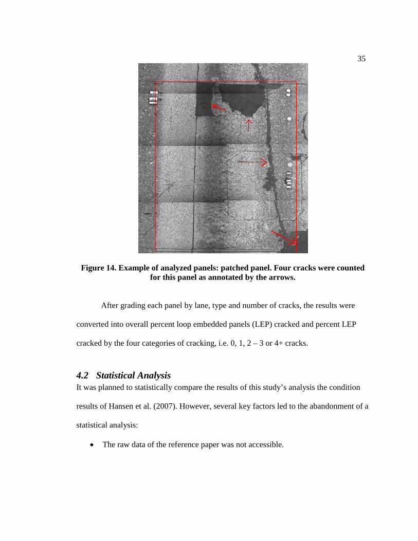
Figure 14. Example of analyzed panels: patched panel. Four cracks were counted for this panel as annotated by the arrows.
After grading each panel by lane, type and number of cracks, the results were
converted into overall percent loop embedded panels (LEP) cracked and percent LEP
cracked by the four categories of cracking, i.e. 0, 1, 2 – 3 or 4+ cracks.
4.2 Statistical Analysis It was planned to statistically compare the results of this study’s analysis the condition
results of Hansen et al. (2007). However, several key factors led to the abandonment of a
statistical analysis:
• The raw data of the reference paper was not accessible.

36
• The difference in sample sizes between the LEP and LFP is big, about 1 LEP to
100 LFP except for the dowel bar rehabilitation and diamond grinding section,
where the ratio is 1 to 30.
• The sample sizes for the reference paper are not given. This required substantial
assumptions to (1) estimate sample size simply by counting the number of lane-
miles in each section, and (2) assume that the standard deviations for both data-
sets are equal.
• The cracking data is not normally distributed making a comparison by t-test
inappropriate.
While these issues could be overcome with effort, it was felt that the resulting
statistics would be more representative of the assumptions made rather than the actual
data. Therefore, statistical analysis was abandoned.
4.3 Traffic Data Handling Vehicle data were aggregated into trucks and others. Trucks were assumed to be long
vehicles and thus the number of trucks was determined by adding bins 2, 3 and 4.
4.4 Traffic Simulation When all the traffic data had been gathered, the vehicle volumes were put into the
VISSIM 5.0 simulation model together with the long vehicle percentage. Those volumes
were assigned to the mainline as well as the off- and on-ramps. Data collection points
were placed where the dual loops are located and then the model was calibrated with the
speed- and volume data from the dual loop detector around NE 145th and NE 110th
street. Data was not collected until after 15 min (900 sec) so the traffic was already

37
flowing in the whole corridor when the collection of data began. The volumes and the
desired speed input were iterated multiple times in order to match actual data. Ten
different random seeds were chosen for the multi-run simulation: 25, 28, 31, 34, 37, 40,
43, 46, 49 and 51. Random Seed initializes the random number generator and due to the
stochastic nature of VISSIM’s simulation model, several simulation runs with different
random seeds are required to compute statistically reliable results (PTV 2008). Once
calibrated against actual data (in terms of volume and speed) two simulations were ran:
(1) near N 163rd street two lanes out of four were closed, and (2) near N 130th street two
out of five lanes were closed. One travel time section was created for the whole corridor
and delay and travel time data was attained with the lanes open and closed for
comparison. After consulting with Martin Dedinsky, traffic engineer at WSDOT, the
closure sections were decided to be 2000 ft and the closure duration was set at four
continuous hours. Figure 15 shows a snap shot of a simulation run.

38
Figure 15. Snap shot of a simulation run.
The assumption was made that no rerouting or trip cancellation would take place,
which is reasonable given the evening/night short duration closures simulated.
Based on travel time sections VISSIM generates delay data for networks. A delay
segment is based on the travel time section. All vehicles that pass the travel time section
are captured by the delay segment, independently of the vehicle classes selected in these
travel time sections.
4.5 Delay Time and Cost from Simulation For the VISSIM simulation program, a delay time measurement is defined as a
“…combination of a single or several travel time measurements; regardless of the
selected vehicle classes, all vehicles concerned by these travel time measurements are
also regarded for delay time measurement. As delay segments are based on travel times

39
no additional definitions need to be done” (PTV 2007). A delay time measurement
determines the mean time delay, compared to the ideal travel time (with no other
vehicles and no signal control) calculated from all vehicles observed on a single or
several link sections.
Travel time is explained in the VISSIM 5.0 user manual as: “Each (road) section
consists of a start and a destination cross section. The average travel time (including
waiting or dwell times) is determined as the time a vehicle crosses the first cross section
to crossing the second cross section. During a simulation run, VISSIM can evaluate
average travel times (smoothed) if travel time measurement sections have been defined
in the network.” Table 7 is an example of a compiled delay data file.
Table 6. Example of compiled data file for delay calculations
Time Delay Stopd Stops #Veh Pers. #Pers
VehC All
No.: 1 1 1 1 1 1
900
14400 149.3 8.3 3.05 7798 149.3 7798
Total 149.3 8.3 3.05 7798 149.3 7798
Where:
• Delay: Average total delay per vehicle (in seconds). The total delay is computed
for every vehicle completing the travel time section, which in this case was the
whole simulation corridor, by subtracting the theoretical (ideal) travel time from
the real travel time. The theoretical travel time is the time that would be reached

40
if there were no other vehicles and no signal controls or other stops in the
network.
• Stopd: Average standstill time per vehicle (in seconds), not including passenger
stop times at transit stops or in parking lots.
• Stops: Average number of stops per vehicle, not including stops at transit stops
or in parking lots.
• #Veh: Vehicle throughput.
• Pers: Average total delay per person (in seconds), not including passenger stop
times at transit stops. Not used for this study.
• #Pers: Person throughput. Not used for this study.
• VehC: Vehicle class. If needed vehicle classed (car truck etc.) can be excluded
from the delay calculation.
• NO: Travel time section number. Only one section used in this simulation.
• 900 – 1400: Beginning and end time of data collection. Data collection began
after 900 seconds of simulation so that the traffic was flowing all over the
corridor.
When construction work-zone reduces the capacity or speed of a section of roadway, the
users will experience longer travel times. These costs are not paid by the owner of the
facility and thus called indirect costs, “paid” by the users in the form of additional time
that the vehicle is in operation and the personal loss of time for the passengers. Since

41
user costs are not a direct cost, rather an indirect cost to society, they are often
overlooked (Wilson and Falls 2003).
The delay cost can be calculated using equations like Caltrans uses:
( ) ( )( )( )CPPTADTISL
RSLhrvehUC
−−= /$ (4-2)
Where
• UC = user delay costs due to construction
• $/vehicle-hour = average value of time due to delay. Typical values applied by
Caltrans as of 2007 include: $10.46/hour for passenger cars and $27.38/hour for
trucks
• L = project length (miles)
• RS = reduced speed through construction zone (mph)
• IS = initial speed prior to construction zone (mph)
• ADT = average daily traffic in current year
• PT = percent of the traffic that will be affected due to construction project
• CP = construction period (days)
In this study, a VISSIM simulation was done to estimate the user delay due to road
closure for installation of the loop detectors. The simulation replaces the equations and
other programs, and should be more accurate because it uses more and better traffic data
and is calibrated. Table 8 shows WSDOT estimates the value of vehicle hours.

42
Table 7. Recommended Dollar Values per Vehicle Hour of Delay Adjusted to 2004 Dollars (WSDOT 2005).
Vehicle Class Value per vehicle hour
Value Range Passenger Vehicles $13.96 $12 to $16
Single-Unit Trucks $22.34 $20 to $24
Combination Trucks $26.89 $25 to $29
The delay data was not available for each vehicle type, so it is assumed that the delay
affects all classes in the same way, i.e. the overall truck percentage in the corridor is
used for single- unit trucks and combination trucks and no distinction made between
them. The traffic data indicates that about 60% of the trucks are combination trucks and
40% single-unit. So the value per vehicle hour for the trucks is:
07.25$89.26%6034.22$%40)/(
..%%)/(
=×+×=−
×+−×−=−
hourvehvalueTruckOr
nvalueCombiCombinunitevalueSinglunitSinglehourvehvalueTruck
5 Data Analysis and Findings Results from the study are presented in this chapter. In the first two sub-chapters (5.1
and 5.2) the results are compared to the condition of the pavement in the whole corridor,
obtained from the reference paper. The next three sub-chapters cover other results of the
cracked (loop embedded) panel data, by type of loop, lane and direction. Finally, the cost
of loop detectors are compared with that of video detectors.

43
5.1 Comparison – Cracked Panels with and without loops Are loop embedded panels (LEP) in worse condition than other loop free panels (LFP)?
In order to be consistent with the corridor condition assessment in Hansen et al. (2007)
results are arranged by rehabilitation technique: non-rehabilitated, diamond ground and
dowel bar retrofitted.
5.1.1 Non-Rehabilitated PCCP Most of I-5 in King County was constructed in the 1960’s and about 83% of it has still
not been rehabilitated. In general, non-rehabilitated PCC pavements show signs of
substantial wheel path wear from studded tires and contain an average of 29% faulted
slabs (Hansen et al. 2007). Table 8 compares average cracking in non-rehabilitated
pavement between all panels in I-5 in King County (data from Hansen et al. 2007) and
the ones embedded with loop detectors (data from this study). Figure 16 shows this
visually.
Table 8. Average Cracking for Non-Rehabilitated
Item
PCC Pavement.
Non-Rehabilitated PCCP
All panels in the corridor (LFP)
# of samples
Loop embedded panels (LEP)
# of samples
NB Mile Posts 139.5 - 177.75 103.75 ln-mi - 139.5 - 177.75
103.75 ln-mi -
SB Mile Posts 139.75 - 177.75 59.05 ln-mi - 139.75 - 177.75
59.05 ln-mi -
No Cracks [%] 86.4 N/A 84.5 538
1 Crack [%] 11.2 N/A 10.4 66
2 - 3 Cracks [%] 2.1 N/A 3.6 23
4+ Cracks [%] 0.3 N/A 1.6 10
% PCCP Cracked 13.6 N/A 15.5 637

44
Figure 16. Average cracking for non-rehabilitated
PCC pavement.
On average there is higher percentage of LEPs cracked than the LFPs. Results by
number of cracks are:
• 1 crack: Slightly fewer LEPs with 1 crack as compared to LFPs.
• 2-3 cracks. LEPs have roughly 70% more cracked panels than LFPs.
• 4+ cracks. There are five times as many LEPs with 4 or more cracks than LFPs.
One possible explanation is that loops do not have much effect on the start of panel
cracking but once a panel is cracked, some characteristic of the loop embedment hastens
the deterioration process and the panel cracks more quickly.
5.1.2 Diamond Ground PCCP At the time of this study (before the WSDOT Triage diamond grinding effort of 2009)
WSDOT had reconstructed about 27 lane miles of I-5 in King County with diamond
grinding. Table 9 compares average cracking in diamond ground pavement between all
diamond ground panels in I-5 in King County (data from Hansen et al. 2007) and the
ones embedded with loop detectors (data from this study). Figure 17 shows this visually.

45
Table 9. Average Cracking for Diamond Ground
Item
PCC Pavement
Diamond Ground PCCP
All panels in the corridor (LFP)
# of samples
Loop embedded
panels (LEP)
# of samples
NB Mile Posts 154.14 - 158.24 14.16 ln-mi - 154.14 - 158.24
14.16 ln-mi -
SB Mile Posts 154.16 - 154.4 12.68 ln-mi - 154.16 - 154.4
12.68 ln-mi -
No Cracks [%] 88.2 N/A 76.8 73
1 Crack [%] 10.7 N/A 15.8 15
2 - 3 Cracks [%] 1.0 N/A 7.4 7
4+ Cracks [%] 0.1 N/A 0.0 0
% PCCP Cracked 11.9 N/A 23.2 95
Figure 17. Average cracking for diamond ground
PCC pavement.
On average there is higher percentage of LEPs cracked than the LFPs. Results by
number of cracks are:
• 1 crack: The fraction of cracked panels is about 50% higher for LEPs than for
LFPs.
• 2-3 cracks. There are seven times as many LEPs with 2-3 cracks than LFPs.

46
• 4+ cracks. There are no LEPs with 4 or more cracks and relatively few (0.1%)
LFPs with 4 or more cracks. This is expected as diamond grinding operations
often replace panels in poor condition.
The sample sizes behind some of those percentages are low, thus the significance of
these results might not be as much as for non-reconstruction however the trends are
similar.
5.1.3 Dowel Bar Retrofit (DBR) At the time of this study, two sections (a total of 6.04 lane-miles) of the study corridor
have been rehabilitated using a dowel bar retrofit (DBR). Table 10 compares average
cracking in DBR between all diamond ground panels in I-5 in King County (data from
Hansen et al. 2007) and the ones embedded with loop detectors (data from this study).
Figure 18 shows this visually.
Table 10. Average Cracking for DBR
Item
PCC Pavement.
Dowel Bar Retrofit and Diamond Grinded PCCP
All panels in the corridor (LFP)
# of samples
Loop embedded
panels (LEP)
# of samples
NB Mile Posts N/A - N/A -
SB Mile Posts 144.45 - 149.69 6.04 ln-mi - 144.45 - 149.69
6.04 ln-mi -
No Cracks [%] 95.6 N/A 97.2 69
1 Crack [%] 4.0 N/A 2.8 2
2 - 3 Cracks [%] 0.4 N/A 0.0 0
4+ Cracks [%] 0.0 N/A 0.0 0
% PCCP Cracked 4.4 N/A 2.8 71
Average age of PCCP as of 2004 39.7 - 39.7 -

47
Figure 18. Average cracking for DBR
PCC pavement.
On average there is lower percentage of LEPs cracked than the LFPs. Results by number
of cracks are:
• 1 crack: The fraction of cracked panels is somewhat less than for LEPs than for
LFPs.
• 2-3 cracks. There are no LEPs cracked.
• 4+ cracks. There are no LEPs or LFPs with 4 or more cracks and relatively few
(0.1%) LFPs with 4 or more cracks. This is expected as DBR operations often
replace panels in poor condition.
The sample sizes behind some of those percentages are low and some previously cracked
panels were replaced in the DBR process, thus these results may be insignificant.
5.2 Comparison – by sections In Hansen et al. (2007) the Washington State Pavement Management System (WSPMS)
was used to identify sections by their year of construction and the type and thickness of
base layers. Thirteen different sections of construction were identified. The results from

48
this study were configured in the same way so the sections could be compared. The
construction years and type and thicknesses of the base layers are displayed in Table 3 in
Chapter 3. Table 11 compares LEPs and LFPs by section.

49
Table 11. Comparing LEPs and LFPs by Section
← N S →
MILE POST NB
174.58-177.75
172.79-174.58
170.85-172.76
170.5 – 170.85
169.18-170.25
167.13-168.34
166.21-167.13
162.68-165.32 N/A 158.24-
162.68 152.65-158.24
149.39-152.65
139.50-149.39
Mile Post SB N/A N/A 170.85-
177.75 170.5 – 170.85
169.18-170.25
167.72-168.34 N/A 162.68-
166.36 160.17-162.68
157.47-160.07
153.15-158.45
149.40-153.15
139.50-149.40
% of Cracked panels
(all panels)
17.4 17.7 20.0 16.3 11.1 11.3 4.4 15.6 13.8 8.5 18.5 17.7 5.5
% of Cracked
LEP 19.6 34.4 19.6 7.1 10.0 18.5 0.0 27.8 26.7 17.6 19.0 10.0 5.5
Sample size of LEP 56 32 92 14 30 27 14 36 30 108 126 40 200

50
Figure 19. Comparing LEPs and LFPs by section.
The sections vary in length, the longest section is about 10 miles and the shortest less
than a mile, so the number of panels (sample sizes) in each section are different. The
LEPs have higher percentage of cracking in 7 of the 13 sections. In three sections the
LFPs have higher percentage of cracking. It seems that LEPs perform worse compared
to LFPs from mileposts 158 – 165; the section around and north of King County Airport
(Boeing Field). No apparent correlations exist between cracking and any data contained
in Table 3 (construction year, number of lanes, base type, base thickness).
5.3 Results – by type of loop There are three types of loops in the study corridor, circle loops, rectangle loops with
soft corners and rectangle loops with sharp corners. In some places in the corridor two or
more loops have been installed in the same panel (called a “loop combo” in this report).
The trend has been to soften the corner of the slots and since 1997 WSDOT only installs
circle loops on the freeway. The main reason for this is that the sharp corners can
damage the chopper wire in the loop detector, making it useless. Other reason is that it is

51
known that sharp corners in concrete create stresses and therefore it is more likely to
crack. The number of cracks by loop type is shown in Table 12 and Figure 20.
Table 12. Number of Cracks in LEPs by Type of Loop Detector
Item Circle loops
Rectangle loops Soft corners
Rectangle loops sharp corners
Loop Combo
All types of loops
No Cracks 92.0 81.0 81.8 92.3 84.8
1 Crack 7.4 10.5 13.4 3.1 10.3
2 - 3 Cracks 0.5 6.3 3.8 1.5 3.6
4+ Cracks 0.0 2.1 1.0 3.1 1.2
% PCCP Cracked 8.0 19.0 18.2 7.7 15.2
First installed 1997 - 2000 Mid 80's Mid 60's N/A N/A
# of samples 188 237 313 65 803
Figure 20. Number of cracks in LEPs by type of loop detector.
There is a significant confounding effect that makes direct comparison by loop type
difficult: loop type is highly correlated with the age of a loop (e.g., circle loops were
installed most recently so are younger than rectangle loops, etc.). Thus, of the three types
of loops the circle loop performs best as would be expected since they were installed

52
fairly recently. Surprisingly, the soft corner rectangle loops exhibit more overall
cracking than the sharp corner rectangle loop even though they were installed on average
20 years later. Explanations for this could be: (1) it is better to saw-cut the pavement
when it is new than is to do it many years after construction, or (2) the soft corner
rectangular loop installations were not done correctly (e.g., saw cuts too deep). Another
rather unexpected result is that the panels with loop combo (2 or more loops) perform
overall very well, even better than the circle type. The reason for this could be that the
location of a new cut is not random (i.e., a LEP is not cut again if it is already cracked.
However, the severity of cracked loop combo panels is high (they have the highest
percentage of 4+ cracks). This could mean that when a panel with a loop combo cracks,
panel deterioration occurs more rapidly than other types. It is difficult to assign cause to
the types of loop cuts in loop combo panels since combinations vary greatly.
5.4 Results – by lane Most of I-5 in King County has 4 lanes in each direction. It is interesting to see how the
panel cracking varies by lane.
Table 13. Percentage of Cracked LEPs by Lane and Rehabilitation Type.
Non-Rehabilitated
PCCP Diamond Ground
PCCP Dowel Bar Retrofit and
Diamond Grinded PCCP Total – With and
without Rehabilitation
%
Cracked LEP
Samples %
Cracked LEP
Samples % Cracked LEP Samples % Cracked
LEP Samples
Lane 1 16.3 123 34.8 23 0.0 18 16.5 164
Lane 2 18.9 159 31.8 22 5.9 17 19.2 198
Lane 3 15.1 179 24.0 25 5.6 18 15.3 222
Lane 4 12.5 176 4.0 25 0.0 18 10.5 219

53
Figure 21. Percentage of cracked LEPs by lane and rehabilitation type.
It is hypothesized that lanes with the highest truck traffic (including buses) will have a
higher fraction of LEPs with cracks. To test this hypothesis, a small sample of truck
traffic by lane was taken on southbound I-5 at NE 145th Street and NE 110th Street. On
these locations there are 4 and 5 lanes respectively. The sample was taken in August
2006 and contained 4 hours of average evening (8:00 pm – 12:00 am), 4 hours of
average weekday (Monday – Wednesday from 6:00 am to 12:00 pm) and 4 hours of
average weekend (Saturday and Sunday 12:00 pm – 16:00 pm) traffic. Traffic volume
was not taken into account, just the ratio between small vehicles and trucks (including
buses) and simple averages were taken from these three time periods and the results are
shown in Table 14.

54
Table 14. Percent Truck Traffic by Lane
145th Average (4 lanes)
110th Average (5 lanes)
% Trucks % Trucks
Lane 1 4.0 2.6
Lane 2 8.9 5.9
Lane 3 2.4 8.6
Lane 4 3.5 3.3
Lane 5 N/A 3.3
LEP cracking tracks with truck traffic reasonably well with Lane 2 having the highest
truck traffic and highest percentage of cracked LEPs. Other confounding elements are:
(1) if lane 4 is an HOV lane it may have been constructed more recently, and (2) trucks
tend to avoid drop lanes and off-ramp cues. As stated the diamond ground LEPs show
big percentages of cracking.
Table 15 and Figure 22 show the number of cracks by lane without regard to
rehabilitation method.
Table 15. Number of Cracks by Lane
1 Crack 2 - 3 Cracks 4+ Cracks
% samples % samples % samples
Lane 1 10.4 17 5.5 9 0.6 1
Lane 2 15.7 31 2.5 5 1.0 2
Lane 3 10.4 23 4.1 9 0.9 2
Lane 4 5.5 12 2.7 6 2.3 5

55
Figure 22. Number of cracks by lane.
The results for 1 crack per panel is very similar to the overall percentage of cracked
panels but for 2-3 cracks there is a spike in lane 3 which might not be expected. The
most unexpected result is in 4+ cracks, lane 4 has the highest percentage of 4 or more
cracks per panel. If sample size were increased (here the sample size is low) it is
unknown if this trend would still be prevalent.
5.5 Results – by direction It is interesting to see if either the northbound or southbound direction is in worse shape
than the other. Differences may indicate trends in truck loading (e.g., more empty trucks
in one direction and more loaded trucks in the other). Table 16 and Figure 23 show
cracked LEPs for northbound and southbound directions by lane.

56
Table 16. Cracked LEPs by Lane and Direction
With and without rehabilitation
NB % of cracked LEP NB # of LEP SB % of
cracked LEP SB # of LEP
Lane 1 20.0 90 12.2 74
Lane 2 25.3 95 13.6 103
Lane 3 19.4 108 11.4 114
Lane 4 8.4 107 12.5 112
All lanes 18.0 400 12.4 403
Figure 23. Cracked LEPs by lane and direction.
With the exception of lane 4, the northbound direction is in significantly worse shape
than the southbound. One hypothesis to explain these results is that truck traffic in the
northbound direction is higher. To test this hypothesis, a small sample of truck traffic by
direction was taken on northbound and southbound I-5 at NE 145th Street. There are five
lanes on this location in the northbound direction compared to four in the southbound
direction. As with the previous truck sample, the sample was taken in August 2006 and
contained 4 hours of average evening (8:00 pm – 12:00 am), 4 hours of average weekday
57
(Monday – Wednesday from 6:00 am to 12:00 pm) and 4 hours of average weekend
(Saturday and Sunday 12:00 pm – 16:00 pm) traffic. Traffic volume was not taken into
account, just the ratio between small vehicles and trucks (including buses). Results
show there were 9.4% trucks in the northbound direction compared to 5.3% trucks for
the southbound direction for the sample times. This gives some indication that there may
be more truck traffic in the northbound direction, which the LEP cracking data seems to
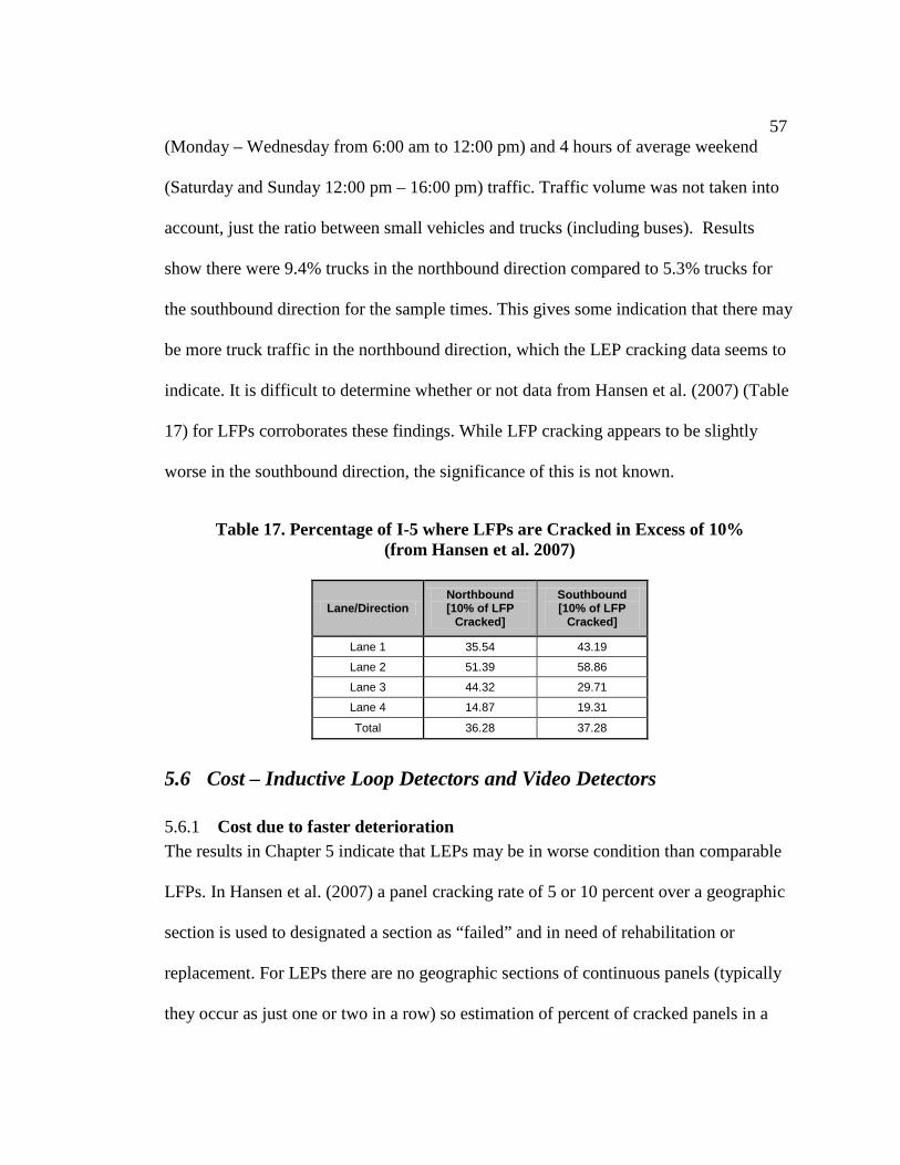
indicate. It is difficult to determine whether or not data from Hansen et al. (2007) (Table
17) for LFPs corroborates these findings. While LFP cracking appears to be slightly
worse in the southbound direction, the significance of this is not known.
Table 17. Percentage of I-5 where LFPs are Cracked in Excess of 10%
(from Hansen et al. 2007)
Lane/Direction Northbound [10% of LFP
Cracked]
Southbound [10% of LFP
Cracked]
Lane 1 35.54 43.19
Lane 2 51.39 58.86
Lane 3 44.32 29.71
Lane 4 14.87 19.31
Total 36.28 37.28
5.6 Cost – Inductive Loop Detectors and Video Detectors
5.6.1 Cost due to faster deterioration The results in Chapter 5 indicate that LEPs may be in worse condition than comparable
LFPs. In Hansen et al. (2007) a panel cracking rate of 5 or 10 percent over a geographic
section is used to designated a section as “failed” and in need of rehabilitation or
replacement. For LEPs there are no geographic sections of continuous panels (typically
they occur as just one or two in a row) so estimation of percent of cracked panels in a

58
section is not possible. Therefore, the definition of “failure” for a LEP is a panel that has
two or more cracks. To evaluate the cost to pavement when installing a loop detector, it
is considered most reasonable to look at non-rehabilitated pavement only and not the
sections with diamond ground and dowel bar retrofit because those rehabilitations were
done only recently, and enough experience has not been gained to evaluate the
pavements lifespan of those sections for the overall cost due to cracked panels.
Calculations for the increased pavement cost due to loop installations are shown in Table
19.
Table 18. Calculations Increased Pavement Costs due to Loop Installations
2+
cracks [%]
# of LEP [Non-rehab]
Cost of panel
replacement [$]
# of panels to be replaced
Cost per LEP [$]
Loop Embedded
Panels (LEP) 5.2 637 20,000 33 1040
Loop Free Panels (LFP) 2.4 637 20,000 15 480
Difference 2.8 - - 18 560
Calculation method: The percentages of panels with two or more cracks were calculated and the difference between LEP and LFP found. Then that number was multiplied by the number of LEP and that gave a theoretical number of additional panels that would have to be replaced because of loop installation. To find cost the panel replacement cost is multiplied by the number of extra panels that is needed to replace and to get the cost for each LEP or each loop that number was divided by the total number of LEPs. Calculation: %8.2%4.2%2.5 =− more LEP with 2+ cracks than LFP 18637%8.2 =× more panels cracked due to loop installation 560$637/000,20$18 =× the extra cost due to loop installation

59
5.6.2 User Cost due to Loop installations To calculate the user cost (cost of delay) of installing loop detectors, two lanes (or three
when there were 5 lanes) at a time were closed in the simulation program. First the delay
was obtained from the program with all lanes open and then with the designated number
of lanes closed. It was assumed that two lanes would remain open at all times. This
resulted in first closing lanes 1 and 2 and then lanes 3 and 4. For the location that had 5
lanes, lanes 1 and 2 were closed and then lanes 3, 4 and 5. Table 20 and 21 show the
results.
Table 19. Lane Closure Results for 4 Lanes
Delay [sec]
Stopd [sec]
Stops [number of]
average travel time [sec] #Veh Total Delay
[Veh-hour]
Lane 1 and 2 closed 148.4 9.1 3.1 383.0 7850 323.5
Lane 3 and 4 closed 294.1 22.3 7.2 528.9 7980 652.0
Average from the
two cloures 221.3 15.7 5.2 455.9 7915 486.4
All lanes open 8.9 0.00 0.0 243.1 8668 21.3
Difference 212.4 15.7 5.2 212.8 -753 465.1
Table 20. Lane Closure Results for 5 Lanes
Delay [sec]
Stopd [sec]
Stops [number of]
average travel time [sec] #Veh Total Delay
[Veh-hour]
Lane 1 and 2 closed 12.1 0.0 0.0 246.5 8567 28.8
Lane 3, 4 and 5 closed 206.8 16.4 4.8 442.4 7089 407.2
Average 109.4 8.2 2.4 344.4 7828 238.0
All lanes open 8.9 0.0 0.0 243.1 8668 21.3
Difference 100.5 8.2 2.4 101.3 -840 216.7

60
Lane Closure Results for 4 Lanes Comments. The delay is significantly higher when
lanes 3 and 4 were closed compared with when lanes 1 and 2 were closed, because of
off-ramp traffic that interrupted the mainline flow. Average delay for a two lane closure
is 221.3 sec/veh. The number of vehicle throughput is not the same because when
vehicles are stopped for more than 7 seconds they diffuse. This number can be changed
and 7 seconds were said to be reasonable (Zhang 2008). The difference in delay in veh-
hour is the difference between average delay for two lane closure and when all lanes are
open. This number describes the delay due to the lane closures.
Lane Closure Results for 5 Lanes Comments. When two out of five lanes of the
freeway are closed, the delay does not increase that much, only about 3 sec/veh, but
when three lanes were closed the increase in delay rose nearly 200 sec/veh from when no
lanes were closed.
The cost of each vehicle-hour is estimated by WSDOT to be $13.96 for cars and
after some calculations (shown in Chapter 4.2.6) the average cost of trucks were found
to be $25.07. Trucks, or long vehicles, were calculated to be around 5% of the total
traffic. Tables 21 and 22 show the cost of delay due to lane closures.
Table 21. User Cost for 4 Lane Freeway due to Loop Installations
Ratio in
traffic Delay [veh-
hour] Cost per veh-hour Cost Cost per
loop Car 0.95 465.1 $13.96 $6168 $3084
Truck 0.05 465.1 $25.07 $583 $292
Total 1 - - $6751 $3376

61
Table 22. User Cost for 5 Lane Freeway due to Loop Installations
Ratio in traffic
Delay [veh-hour]
Cost per veh-hour Cost Cost per
loop
Car 0.95 216.7 $13.96 $2874 $1150
Truck 0.05 216.7 $25.07 $272 $109
Total 1 - - $3146 $1258
Assuming that I-5 would be closed to install or replace a loop detector, the user cost
would be about $3,400 for the 4 lane sections and $1,300 for 5 lane sections. These are
theoretical results because WSDOT does not close lanes solely to install or replace loop
detector, but waits for other projects that have to be done on the freeway, and installs the
loops simultaneously.
5.6.3 Video Detectors When estimating the cost of video detector installation it is assumed that no lane
closures have to be made, and therefore no user cost associated with it. The installation
cost without the equipment needed is considered to be 30% of the loop installation cost,
about $300. WSDOT did not have an estimation for this cost item, so this is a rough
estimate made by the author, based on how much work seems to be affiliated, in
proportion to the loop installation.
5.6.4 Cost Comparison – Inductive Loop Detectors and Video Detectors Table 23 shows a comparison between the theoretical costs of loop detection and video
detection assuming maintenance costs are minimal. The average lifetime of loop and
video detector is assumed to be the same based on WSDOT advice (Didensky 2008).

62
Table 23. The Cost of Installing Loop Detectors and Video Detectors
Inductive Loop Detector Video Detector
Equipment cost [$] 500 - 800 5,000 - 26,000
Installation Cost [$] 1,000 300
Cost on the Pavement [$] 560 -
User cost [$] 1,260 - 3,380 -
Total Cost [$] 3,320 - 5,740 5,300 - 26,300
For the loop detectors the user cost is a substantial part of the total cost of loop
installation (about 60% in a four lane freeway and 40% in a five lane freeway). If this
cost is accounted for, a video detector installation may actually result in a lower lifecycle
cost on a 4 lane freeway.

63
6 Conclusions and Recommendations
6.1 Conclusions This study focused on PCC pavement panels with embedded traffic loop detectors
(LEPs) on I-5 in King County and how they are performing in relation to other panels
(i.e., loop free panels, LFPs). Major findings were as follows:
• Results may not be transferrable. Since there are few (if any) studies on LEP
condition it was not possible to verify results of this study with others. It may be
that different study corridors show different results.
• Comparison by cracking. LEPs show poorer performance than LFPs in terms of
cracking except on the small section of I-5 that has been dowel bar retrofitted and
diamond ground.
o Non-rehabilitated PCC pavement
o
. For panels with one crack, the
difference is not much (1 – 2%). However, when considering “failed
panels” (defined as those with 2 or more cracks) the difference between
LEP and LFP is substantial: the fraction of LEPs is twice as high as the
fraction of LFPs. have 2 or more cracks - percent vise – than LFP. This
might indicate that the loop installation tends to influence the severity of
panel cracking rather than the initiation.
Diamond ground PCC pavement. The LEP are in worse condition than
LFP in all categories. Specifically, the fraction of “failed” LEPs (2 or
more cracks) is about seven times the fraction of “failed” LFPs (2 or more
cracks).

64
o Dowel bar retrofit (DBR) PCC pavement
• Comparison by section (see Table 3 for section definition). LEPs have higher
cracked panel fraction in 7 of the 13 sections. In three sections the LFPs have
higher cracked panel fraction (two of these have low samples sizes making the
results less certain). It is difficult to draw any firm conclusions on a section-by-
section basis although it does seem that LEPs perform worse than LFPs from
mileposts 158 – 165 (near and north of Boeing Field).
. There are no “failed” (2 or
more cracks) LEPs in the DBR section and only 0.4% of LFPs are
“failed” (2 or more cracks). This is expected since failed panels are
usually removed and replaced in the DBR process.
• Comparison by loop type. LEPs with circle loops have fewer cracks than those
with rectangular loops. This effect is pronounced in panels with two or more
cracks. This may not be a reasonable comparison because circle loops were
installed much later than the rectangular ones.
• Cost attributable to shorter panel life from loop detector installation. Using
non-rehabilitated PCCP for calculations, the cost due to shorter panel lifetime
because of loop installation is estimated at $560 per loop detector, which is about
25% of the installation cost (this excludes the user cost associated with traffic
delay).
• Cost attributable to traffic delay (user cost). The user cost due to traffic delay
caused by lane closures can be a significant part of the overall cost of loop
installation (around 60% for a 4 lane freeway and about 40% for a 5 lane

65
freeway) if loop installation is the only reason for closing lanes. However, loop
detectors are typically installed when lanes are closed for other reasons.
• Cost comparison between loop and video detectors. When compared for a 4-
lane freeway the inclusion of user costs for loop detector installation makes total
lifecycle costs between loop and video detectors comparable and, in situations
with high traffic and inexpensive video detectors, can sometimes result in video
lifecycle costs being less. While this does not suggest video detectors are
universally less expensive (in fact, they are usually more expensive), it does
indicate that user costs are important to include in comparing detector costs.
6.2 Recommendations The following recommendations are made:
• Continue using circle loop detectors. The shape of loop detectors matters for
performance of the pavement, and even though the comparison between various
shapes may not be accurate because of different installation times, the results
indicate that circle loops have less impact on the panel cracking than rectangular
shapes. WSDOT has realized this and now only uses circle loops for new
installations.
• Even considering potential PCC damage, loop detectors are still a cost
competitive means of traffic detection. The cost comparison between loop and
video detection shows loop detectors are still a more economical solution for
traffic detection than video detectors in most situations. Table 23 shows that the
lifecycle cost of a loop detector is estimated at between $3,320 and $5,740 (with

66
$560 due to increased pavement damage and $1,260 to $3,380 due to user delay).
This compares to the lifecycle cost of a video detector estimated at between
$5,300 and $26,300 (with no cost for pavement damage or user delay). If circle
loops are used the cost due to pavement damage is likely to be even less.
• Further comparison. One other comparison method with potential would be to
compare the LEPs with the adjacent LFPs on either side of the LEP.
• Reevaluate user cost. The simulation for this study used evening traffic volumes
(8 p.m. to midnight) but it may be more reasonable to use early morning volumes
(say, midnight to 5 a.m.). This could potentially result in lower estimated user
costs.
• Compare loop detection to other detection methods beyond video. Other
traffic detection systems may compare differently to loop detectors.

67
References Dedinsky, Martin. (2008). Transportation Engineer, Washington State Department of
Transportation. Email communication July – November 2008.
Hansen, M.A.; Mahoney, J.P.; Jackson, N.C.; Hunter, C.; Pierce, L.M.; Turkiyyah, G.T.
(2007). Assessment of the I-5 Portland Cement Concrete Pavements in King County.
WA-RD 682.1. Washington State Department of Transportation, Olympia, WA.
Ishimaru, J. M. and Hallenbeck, M. E. (1999). Flow Evaluation Design Technical
Report. WA-RD 446.2, Washington Department of Transportation, Olympia, WA.
Muench, S.T.; Ozolin, B.; Uhlmeyer, J. and Pierce, L.M. (2007). Rapid Concrete Panel
Replacement in Washington State: Lessons Learned. International Conference on
Optimizing Paving Concrete Mixtures and Accelerated Concrete Pavement
Construction and Rehabilitation, 7-9 November 2007, Atlanta, GA.
Parametrix (2008). I-5 Pavement Reconstruction and Operations Analysis. PowerPoint
presentation. Washington State Department of transportation (WSDOT).
Pathway Services Inc. (2008). Pathview ІІ. Website. http://www.pathwayservices.com.
Accessed 10 November 2008.
Planung Transport Verkehr AG (PTV). (2008). VISSIM – Integrated multi-run tool.
Website. http://www.ptvamerica.com. Accessed 10 November 2008.
Federal Highway Administration (FHWA). (2006). Traffic Detector Handbook, Third
Edition—Volume I, Publication No. FHWA-HRT-06-108, U.S. Department of
Transportation, Washington, D.C.
University of Washington (UW) (2007). Traffic Data Acquisition and Distribution
(TDAD). An ITS Research Program developed with the sponsorship of WSDOT.
Available on http://www.its.washington.edu/tdad.
Voigt, G.F. (2002). Early Cracking of Concrete Pavement - Causes and Repairs. 2002
Federal Aviation Administration (FAA) Airport Technology Transfer Conference.

68
Wang, Y. and Nihan, N. (2004). Dynamic Estimation of Freeway Large-Truck Volumes
Based on Single-Loop Measurements. Journal of Intelligent Transportation
Systems, Vol. 8, No. 3, 133-141.
Wilson, C.J., Falls, L.C. (2003). Construction Related User Delay Costs – The Case of
the Crowchild Trail Bridge Rehabilitation in Calgary. University of Calgary.
Zhang, G. (2008). Ph.D graduate from the University of Washington. Personal
Conversation, October 2008.