Effects of Including Agricultural Products in the

Customs Union between Turkey and the EU

A Partial Equilibrium Analysis for Turkey

Dissertation

zur Erlangung des Doktorgrades

der Fakultät für Agrarwissenschaften

der Georg-August-Universität Göttingen

vorgelegt von

Harald Grethe

geboren in Buchholz i. d. Nordheide

Göttingen, im April 2003

Gefördert von der Deutschen Forschungsgemeinschaft

This thesis is published under the same title at Peter Lang Publishing Group

(www.peterlang.com). Page numbering and page breaks are identical. Format allows for two

pages on one A4 page printing.

D 7

Referent: Professor Dr. S. Tangermann

Korreferent: Professor Dr. S. von Cramon-Taubadel

Tag der mündlichen Prüfung: 23. Mai 2003

5

ACKNOWLEDGEMENTS

Many people have contributed to this work; they are too numerous to be all mentioned here. The early investigative stages of my work were part of a FAO policy reform project located in Ankara. While working in Turkey, I was supported by many people in gathering information and understanding Turkish agriculture and agricultural policies. To all of them I want to express my thankfulness and my appreciation for their warm hospitality, which I enjoyed so much.

Tayfur Caglayan and his staff members at the Research Planning and Coordination Council of the Ministry of Agriculture and Rural Affairs (MARA) provided much support at the early stage of my work and Don McClatchy was an extremely supportive project leader. Selma Aytüre and Ayse Demirtas at MARA organized many meetings in Ankara, to which they also accompanied me. Many people at the Undersecretariat of Foreign Trade (UFT) provided information on agricultural trade policies. Special thanks are due to Fisun Aktug and her staff members at the General Directorate of EU Affairs (UFT) who helped me to understand the complex structure of preferential trade rules between Turkey and the EU. Ermine Kocberber from the State Institute of Statistics (SIS) and her staff members provided data as of then unpublished, and background information on how data is collected. Sezmen Alper and Buket Teumann at the Exporters' Union at Izmir organized meetings with many traders and processors of agricultural products and provided a great amount of information. Also, thanks are due to Halis Akder and other academics at Ankara whose experience and knowledge of the agricultural sector in Turkey was invaluable.

Later stages of my work were generously supported by the Deutsche Forschungsgemeinschaft. During this time I relied much on unpublished or out-of-print data at the SIS. Especially, Aysun Karabulut at the Agricultural Statistics Division and Özlem Sarica at the Income and Expenditures Division helped me enormously with collecting information, finding my way in SIS, and discussing availability, sample procedures, and reliability of data. I am grateful for their persistent willingness to accept my time-consuming, never-ending questions, and my "data-hunger". Mehmet Azgin at the UFT helped me several times by providing recent and historical data on Turkey’s import tariff schedule. Special thanks are due to Ayse Uzmay at the agricultural faculty of the Aegean University in Izmir, who helped me a great deal with collecting data and more informal information from various sources not always easily accessible.

6

At the Institute of Agricultural Economics in Göttingen, Rainer Marggraf and Stephan v. Cramon-Taubadel made helpful comments as referee at an early stage of the work and as second supervisor, respectively. Jochen Meyer introduced me to econometrics in GAUSS, as did Martin Banse with programming TURKSIM in GAMS. I am grateful for their support. It was especially comforting to know that Martin was just one door away from mine, and in case of seemingly unsolvable "execution errors" it always helped to enter his room with a desperate expression on my face. Susanne Hagge supported me in the cumbersome task of data processing. And, during the last stage of the work, Stephan Nolte efficiently helped me with various small and large last minute problems. Martin Banse, Fritz Feger, and Andrea Wälzholz read parts of the manuscript. I am grateful for all their thorough comments and suggestions as well as their readiness for long and fruitful discussions throughout my time in Göttingen. Petra Geile and Ann Hartell both read the manuscript completely and thoroughly checked on language and editorial aspects. To all of them, and many others not listed here, I want to express my gratitude. Remaining errors, of course, are mine.

Special thanks are due to Stefan Tangermann my academic teacher, who supervised my dissertational work. I am grateful for his advice, constructive criticism, and support, and his enormous and sustained readiness to discuss and think things through continuously, which contributed a lot to such a pleasant time in Göttingen, also beyond the work on my thesis.

Final thanks to my wife Kathelijne, who took over a great deal of my share in family tasks, especially during the last year of my work on this project.

Bühren, December 2003 Harald Grethe

7

PREFACE

While the European Union is in the process of implementing its largest round of enlargement ever, to include ten new Member countries from mainly Central Europe, consideration is already being given to the possibility of entering into accession negotiations with Turkey. For the time being it is plainly impossible to predict the future fate of a possible membership of Turkey in the European Union, but there is no doubt that this is a politically highly significant project for both sides. However, it is relatively safe to forecast that the economic relationships between Turkey and the European Union will in any case intensify in the years to come. One important factor in the economic links between Turkey and the EU is the Customs Union between the two sides, in force since 1996.

The Customs Union does not yet extend to agricultural products. However, significant parts of agricultural trade between the two partners are already covered by various forms of preferences. Moreover, the agreement that established the Customs Union requires both sides to work towards a progressive extension of such preferential treatment in the agriculture sector. It also, interestingly, commits Turkey to bringing its agricultural policies in line with the EU’s Common Agricultural Policy where necessary to allow for a free flow of such preferential trade. All these commitments to make further progress on bilateral trade in agriculture, though, are not really firm, and a timetable was not established. Yet, it is well conceivable that the dynamics of progressing on the front of agricultural trade might intensify in the future, as one element of the ongoing process of strengthening the political and economic ties between Turkey and the European Union. The end point of a full inclusion of agriculture in the Customs Union is certainly one possible option in this process.

For Turkey, where agriculture plays an important role in the overall economy and for the social fabric in rural regions, such a development could have significant implications. Yet, what precisely the impacts of a full inclusion of agriculture in the Customs Union might be is a matter of debate. Would agriculture in Turkey come under strong pressure as a result of competition from farmers in the EU? Or are there gains to be made for Turkey’s farmers, from gaining better access to the EU market? Which agricultural products would fall into which of these two alternative categories? How would the different regions in Turkey be affected? Would pressures arise to adjust agricultural policies in Turkey to those of the EU? And if so, what are the options? How would the overall economy fare?

8

Questions like these can only be answered on the basis of a careful empirical analysis, and the complexity of agricultural markets with the close substitution and complementarity relationships across products have to be considered as well as the specifics of price formation in the context of changing trade flows. At the same time the requirement of adopting appropriate policy measures has to be kept in mind, at both the domestic level in Turkey and in the context of the international commitments in the framework of the World Trade Organization.

In his doctoral dissertation that is published here, Harald Grethe has not shied away from the demanding task of including all these complexities in his analysis of the issues. He has dealt in a competent manner with both the quantitative analysis of the market and welfare implications and the ramifications for agricultural policy making and international trade policy. The research presented here is based on extensive knowledge of the situation on the spot in Turkey, and has benefited from the insights of the many colleagues in Turkey with whom Harald Grethe has cooperated. The concrete results achieved, but also the analytical approaches adopted should prove valuable in future decision making on these issues.

Paris, December 2003 Stefan Tangermann

9

CONTENTS

List of Tables ........................................................................................... 15 List of Graphs .......................................................................................... 21 List of Figures .......................................................................................... 21 Abbreviations........................................................................................... 23 Executive Summary ................................................................................. 25

1 INTRODUCTION............................................................................................. 27

2 AGRICULTURAL MARKETS AND POLICIES IN TURKEY AND THE EUROPEAN UNION ........................................................................................ 31

2.1 Introductory Overview .................................................................... 31

2.2 Agricultural Markets and Product-Specific Support Policies ..... 33 2.2.1 Cereals ......................................................................................... 33 2.2.2 Other Crops.................................................................................. 36 2.2.3 Fruit and Vegetables .................................................................... 39 2.2.4 Meat ............................................................................................. 45 2.2.5 Eggs and Milk.............................................................................. 49

2.3 Non-Product-Specific Agricultural Policies................................... 52

3 DEVELOPMENT AND STATUS OF AGRICULTURAL TRADE RELATIONS BETWEEN TURKEY AND THE EUROPEAN UNION ......................................... 53

3.1 Overview of Agricultural Trade between Turkey and the European Union................................................................................ 53

3.2 Agricultural Trade Preferences between Turkey and the European Union................................................................................ 57

3.2.1 EU Preferences Granted for Agricultural Products Originating from Turkey ............................................................. 57

3.2.2 Turkish Preferences Granted for Agricultural Products Originating from the EU.............................................................. 63

3.2.3 Preferential Trade Arrangements for Non-Annex I Products ..... 65

10

4 FUTURE AGRICULTURAL TRADE RELATIONS BETWEEN TURKEY AND THE EU: THE POTENTIAL INCLUSION OF AGRICULTURE IN THE CUSTOMS UNION .......................................................................................... 69

4.1 Theoretical Aspects of a Customs Union in Agriculture between Turkey and the EU............................................................ 69

4.1.1 Comparative Static Effects .......................................................... 69 4.1.2 Dynamic Effects of Market Integration....................................... 71

4.2 Previous Analytical Work on the Integration of Agricultural Markets between Turkey and the EU ............................................ 72

4.3 Institutional Aspects of a Customs Union in Agriculture between Turkey and the EU............................................................ 75

4.3.1 Harmonization of Agricultural Price Policies and Prices............ 75 4.3.2 Harmonization of Other Agricultural Policies ............................ 76 4.3.3 WTO Aspects............................................................................... 77

4.3.3.1 Market Access ....................................................................... 79 4.3.3.2 Export Competition............................................................... 81 4.3.3.3 Domestic Support.................................................................. 84

5 QUALIFICATION AND STRUCTURE OF THE TURKISH AGRICULTURAL SECTOR MODEL FOR POLICY ANALYSIS..................................................... 89

5.1 Potential Modeling Tools for the Analysis of the Extension of the Customs Union and Justification of the Chosen Model..... 89

5.2 Overview of the Turkish Agricultural Sector Model.................... 93

5.3 Integration into the International Trade Environment ............. 102 5.3.1 Basic Approach.......................................................................... 102 5.3.2 The Generation of Border Prices and the Link to the

Domestic Price Level in the Base Situation .............................. 104 5.3.3 The Generation of Border Prices and the Link to the

Domestic Price Level in Simulations ........................................ 107

5.4 Farm Supply Model ....................................................................... 108 5.4.1 Plant Products ............................................................................ 109

5.4.1.1 Basic Mechanisms............................................................... 109 5.4.1.2 Additional Irrigation Area................................................... 110

5.4.2 Animal Products ........................................................................ 112

11

5.5 Feed Model ...................................................................................... 114

5.6 Processing Model............................................................................ 115

5.7 Demand Model................................................................................ 115

5.8 Welfare Calculations...................................................................... 116 5.8.1 Welfare Changes at Farm Level ................................................ 116 5.8.2 Welfare Changes at the Consumer Level .................................. 121 5.8.3 Welfare Changes at the Level of the Processing Industry......... 121 5.8.4 Budgetary Effects ...................................................................... 121

6 BEHAVIORAL PARAMETERS....................................................................... 123

6.1 Basic Approach............................................................................... 123

6.2 Supply Side...................................................................................... 124 6.2.1 Plant Products ............................................................................ 124

6.2.1.1 Determination of Own Price Elasticities and Cost Shares of Variable Inputs .................................................... 126

6.2.1.2 Determination of Cross Price Elasticities ........................... 129 6.2.2 Animal Products ........................................................................ 131

6.3 Demand Side ................................................................................... 133 6.3.1 Estimation of Income Elasticities from Expenditure

Survey Data................................................................................ 133 6.3.1.1 Basic Considerations on the Use of Income Elasticity

Estimates Based on Cross-Section Expenditure Data for Agricultural Sector Models ........................................... 134

6.3.1.2 Data Set ............................................................................... 138 6.3.1.3 Estimation Method and Results .......................................... 149

6.3.2 Development of Elasticity-Matrices of Human Demand for Each Income Quintile ................................................................ 152

6.3.2.1 Determination of Income and Own Price Elasticities......... 153 6.3.2.2 Determination of Cross Price Elasticities ........................... 158

6.3.3 Development of Elasticity-Matrices of Feed Demand .............. 158 6.3.4 Determination of Processing Demand Elasticities .................... 159

6.4 Estimation of Price Transmission Elasticities for Animal Products........................................................................................... 160

12

7 DATA SET FOR MODEL CALIBRATION ...................................................... 167

7.1 Supply, Trade, and Demand ......................................................... 167 7.1.1 Supply ........................................................................................ 167

7.1.1.1 Standard Approach.............................................................. 167 7.1.1.2 Specific Cases ..................................................................... 167

7.1.2 Trade .......................................................................................... 170 7.1.3 Demand...................................................................................... 171

7.1.3.1 Processing Demand, Seed Demand, and Waste.................. 171 7.1.3.2 Feed Demand....................................................................... 171 7.1.3.3 Human Demand................................................................... 173

7.2 Domestic Prices, Trade Prices, and Margins............................... 175 7.2.1 Domestic Prices ......................................................................... 175 7.2.2 Trade Prices ............................................................................... 176 7.2.3 Margins ...................................................................................... 176

7.3 Base Period Policies........................................................................ 177 7.3.1 Tariffs......................................................................................... 177 7.3.2 Export Subsidies ........................................................................ 177 7.3.3 Producer Premiums.................................................................... 178

8 PROJECTION SCENARIOS ........................................................................... 179

8.1 World Market Prices ..................................................................... 180

8.2 Shifters at the Supply Side ............................................................ 182

8.3 Shifters at the Demand Side .......................................................... 183

8.4 Development of the Southeast Anatolian Irrigation Project ..... 183

8.5 Policies and Price Formation under the Status Quo and the Liberalization Scenario.................................................................. 185

8.6 Policies and Price Formation under the CU Scenario ................ 186

13

9 RESULTS OF POLICY SIMULATIONS........................................................... 191

9.1 Effects on Agricultural Prices, Production, and Consumption................................................................................... 191

9.1.1 National Effects Aggregated per Product Group....................... 191 9.1.2 National Effects per Product...................................................... 197 9.1.3 Production Effects per Region and Consumption Effects

per Income Quintile ................................................................... 201

9.2 Effects on Trade ............................................................................. 203

9.3 Welfare Effects ............................................................................... 206 9.3.1 Effects on Producer and Consumer Welfare ............................. 206 9.3.2 Effects on Budgetary Outlays and Revenue and Overall

Welfare Effects .......................................................................... 210 9.3.3 Effects on Welfare Distribution................................................. 213

9.3.3.1 Changes in Producer Surplus per Region ........................... 213 9.3.3.2 Change in Consumer Welfare per Income Group............... 218

9.4 Impact of Changes in Farmgate-Wholesale Price Margins and the Real Exchange Rate.......................................................... 219

10 CONCLUSIONS ............................................................................................ 223

10.1 Liberalization of the Agricultural Sector..................................... 223

10.2 Extension of the Customs Union with the EU to Cover Agricultural Products .................................................................... 226

REFERENCES ..................................................................................................... 229

ANNEX ............................................................................................................... 237

to Chapter 3 Overview of Existing Preferences Granted by the EU for Agricultural Imports Originating in Turkey .......................................... 239

to Chapter 5 TURKSIM GAMS code ........................................................................ 255

to Chapter 6 Table A-6.1: Allen Substitution Elasticities of Area Allocation ........... 285 Tables A-6.2-10: Regional Price Elasticities of Area Allocation.......... 286

14

Tables A-6.11-19: Regional Price Elasticities of Animal Supply ......... 295 Table A-6.20: Allen Substitution Elasticities of Human Demand ........ 297 Tables A-6.21-25: Compensated Price Elasticities of Human Demand per income quintile.................................................................. 298 Tables A-6.26-30: Allen Substitution Elasticities of Feed Demand ..... 303 Tables A-6.31-35: Price Elasticities of Feed Demand........................... 304

to Chapter 7 Tables A-7.1-A-7.4 (Base data) ............................................................. 305

to Chapter 8 Tables A-8.1-A-8.3 (price data for scenarios) ....................................... 311

to Chapter 9 Table A-9: Results per product .............................................................. 314

other Map of Production Regions in Turkey .................................................. 335

15

LIST OF TABLES Table 2.1: Overview of the Agricultural Sectors in Turkey and the EU

(bill. €, 1999/00) ................................................................................ 31 Table 2.2: Comparison of Producer Support Estimates in Turkey and

the EU................................................................................................ 32 Table 2.3: Market Data for Cereals (1999/00) .................................................... 34 Table 2.4: Cereal Farmgate Prices in Turkey and the EU (€/t)........................... 36 Table 2.5: Market Data for Selected Crops (1999/00)........................................ 37 Table 2.6: Crop Prices in Turkey and the EU (€/t) ............................................. 38 Table 2.7: Market Data for Fruit (1999/00) ........................................................ 40 Table 2.8: Market Data for Vegetables (1999/00) .............................................. 41 Table 2.9: Fruit and Vegetables Covered by the EU Entry Price System .......... 42 Table 2.10: Turkish and EU Prices for Fruit and Vegetables Covered by

the EU Entry Price System (€/t) ...................................................... 43 Table 2.11: Prices for Olives and Olive Oil in Turkey and the EU (€/t) ............ 45 Table 2.12: Market Data for Meat (1999/00)...................................................... 46 Table 2.13: Meat Prices in Turkey and the EU (€/t) ........................................... 47 Table 2.14: Market Data for Eggs and Dairy (1999/00) ..................................... 49 Table 2.15: Egg and Dairy Prices in Turkey and the EU (€/t)............................ 51 Table 3.1: Trade Overview of Turkey and the EU (bill. €) ................................ 53 Table 3.2: Composition of Turkish Agricultural Imports by Origin

(percent)............................................................................................. 55 Table 3.3: Composition of Turkish Agricultural Exports by Destination

(percent)............................................................................................. 56 Table 3.4: Classification of Turkish Agricultural Exports to the EU

According to the EU's Import Regime, 2001 (€1,000) ..................... 59 Table 3.5: Fruits and Vegetables Subject to a Seasonal ad valorem Tariff ........ 61 Table 3.6: TRQ for Turkish Exports to the EU, Utilisation of TRQ and

Tariff Rates ........................................................................................ 62 Table 3.7: Selected TRQs for EU Exports to Turkey, Quota Utilization

and Tariffs ......................................................................................... 64 Table 3.8: Preferences Granted by Turkey for Agricultural Imports

Originating from the EU, 2002 ......................................................... 65

16

Table 3.9: Trade of Table-2 and Non-Annex I Products between Turkey and the EU (mill. €) ........................................................................... 67

Table 4.1: Comparative Static Effects of Free Trade and a CU on Turkish Agriculture (Grethe, 1999) ................................................................ 74

Table 4.2: Comparative Static Effects of a CU on Turkish Agriculture (Cakmak and Kasnakoglu, 2001) ...................................................... 75

Table 4.3: Agricultural Products for which EU Tariff Bindings in the WTO Exceed those of Turkey........................................................... 80

Table 4.4: Comparison of Product Groups Specified by Turkey, the EU, and the WTO Modalities ................................................................... 82

Table 4.5: Turkish and EU Budgetary Outlays for Export Subsidies................. 83 Table 4.6: Implicit Export Subsidies, 2000......................................................... 83 Table 4.7: Bound and Notified EMS Compared to Alternative

Calculations (percent of production value) ....................................... 87 Table 5.1: Overview of Equations in the TURKSIM Core Model ..................... 96 Table 5.2: Product Coverage and Activities in TURKSIM ................................ 99 Table 5.3: Value Shares of Products Covered by TURKSIM (1999)............... 101 Table 5.4: Parameters and Sets Used for Establishing a Link between

Domestic and Border Price.............................................................. 105 Table 6.1: Own Price Elasticities, Cost Shares of Variable Inputs, and

the Resulting Supply Elasticities with Respect to the Variable Input Prices...................................................................................... 127

Table 6.2: Own Price Elasticities, Cost Shares of Variable Inputs and Feed, and the Resulting Supply Elasticities with Respect to the Variable Input Prices and the Feed Price .................................. 131

Table 6.3: Allen Elasticities of Cross Substitution in Production of Animal Products .............................................................................. 133

Table 6.4: Products Covered by Demand Analysis .......................................... 139 Table 6.5: Income and Total Expenditure Per Capita by Income Quintile

(1994, mill. TL) ............................................................................... 141 Table 6.6: Results of Estimation of Engel Curves ............................................ 151 Table 6.7: Elasticities of Demand with Respect to Total Expenditures,

Estimation Results ........................................................................... 152 Table 6.8: Income Elasticities in TURKSIM.................................................... 154

17

Table 6.9: Own Price Elasticities in TURKSIM............................................... 157 Table 6.10: Calculation of Processing Demand Elasticities of the

Sunflower Seed Crushing Industry................................................ 160 Table 6.11: Processing Demand Elasticities ..................................................... 160 Table 6.12: Turkish Import, Border, and Domestic Prices for Beef (US$/t).... 161 Table 6.13: Turkish Import, Border, and Domestic Prices for Dairy

Products (US$/t) ............................................................................ 163 Table 6.14: Estimation of Price Transmission Elasticities for Beef

and Milk ......................................................................................... 165 Table 7.1: Number of Fruit Trees...................................................................... 168 Table 7.2: Tomato Paste Production Quantities and Prices, 1997-2001........... 169 Table 7.3: Olive Oil Production Quantities, 1997-2001 ................................... 169 Table 7.4: Base Period Feed Demand ............................................................... 172 Table 7.5: Nutrient and Value Shares of Coarse Feed in Total Feed for

Ruminants........................................................................................ 173 Table 7.6: Total Expenditure and Food Expenditure per Income Quintile ...... 174 Table 7.7: Products with Implicit Export Subsidies ......................................... 177 Table 8.1: World Market Price Projections and Assumed Changes in

Real World Market Prices for TURKSIM, 1996/98 to 2006 (percent)........................................................................................... 181

Table 8.2: Growth Rates 1968 to 1998 and Assumed Productivity Shifter...... 182 Table 8.3: Classification of Products into Irrigation Indices ............................ 184 Table 8.4: Parameters irr_w .............................................................................. 184 Table 8.5: Projections of Crop Pattern on Irrigated GAP Area (percent)......... 185 Table 8.6: Assumptions on Policies and Price Formation under the

CU Scenario..................................................................................... 187 Table 9.1: Price, Production, and Consumption Changes: Status Quo

Scenario (2006) Compared to the Base Situation (1997/99), (percent)........................................................................................... 192

Table 9.2: Price and Production Changes at Farm Level: Liberalization and CU Scenarios Compared to the Status Quo Scenario (2006), (percent) .............................................................................. 194

18

Table 9.3: Price and Consumption Changes at Wholesale Level: Liberalization and CU Scenarios Compared to the Status Quo Scenario (2006), (percent) ............................................................... 196

Table 9.4: Price, Production and Consumption Changes: Liberalization and CU Scenarios Compared to the Status Quo Scenario (2006), (percent)........................................................................................... 198

Table 9.5: Changes in Feed Cost Indices (percent) .......................................... 200 Table 9.6: Changes in Prices and Quantities of Products of the Oil Seed

Crushing Industry (percent)............................................................. 200 Table 9.7: Changes of Production Value, per Region (percent) ....................... 201 Table 9.8: Changes in Food Consumption Quantity and Expenditure, per

Income Quintile (percent) ............................................................... 203 Table 9.9: Net Trade by Product Group under Different Scenarios (mill. €) ... 204 Table 9.10: Net Trade, per Product (1,000 t) .................................................... 205 Table 9.11: Change in Total Producer Surplus and Consumer Welfare........... 207 Table 9.12: Change in Producer Surplus and Consumer Welfare, per

Product ........................................................................................... 209 Table 9.13: Budgetary Revenue (mill. €).......................................................... 210 Table 9.14: Total Welfare Effects (mill. €)....................................................... 211 Table 9.15: Terms of Trade and Allocation Effect of a CU, (mill. €) .............. 212 Table 9.16: Calculation of the Allocation Effect of a CU, (mill. €) ................. 212 Table 9.17: Impact of Shifters on Terms of Trade Effect under a CU ............. 213 Table 9.18: Change in Regional Producer Surplus (mill. € and percent of

production value) ........................................................................... 214 Table 9.19: Distribution of Farms by Area and Region, 1991.......................... 215 Table 9.20: Distribution of Changes in Producer Surplus for Wheat

among Farm Size Groups (percent)............................................... 217 Table 9.21: Distribution of Farms, Area, and Ruminants, by Farm Size

and Region, 1991 ........................................................................... 217 Table 9.22: Change in Consumer Welfare by Income Quintile........................ 218 Table 9.23: Effects of Decreasing Farmgate-Wholesale Price Margins,

(mill. €) .......................................................................................... 220 Table 9.24: Effects of Real Devaluation and Appreciation of the

Turkish Lira ................................................................................... 222

19

ANNEX TABLES Table A-6.1: Allen Substitution Elasticities of Area Allocation ..................... 285 Table A-6.2: Price Elasticities of Area Allocation, North Central ................... 286 Table A-6.3: Price Elasticities of Area Allocation, Aegean ............................. 287 Table A-6.4: Price Elasticities of Area Allocation, Europe.............................. 288 Table A-6.5: Price Elasticities of Area Allocation, Mediterranean .................. 289 Table A-6.6: Price Elasticities of Area Allocation, Northeast.......................... 290 Table A-6.7: Price Elasticities of Area Allocation, Southeast.......................... 291 Table A-6.8: Price Elasticities of Area Allocation, Black Sea ......................... 292 Table A-6.9: Price Elasticities of Area Allocation, East................................... 293 Table A-6.10: Price Elasticities of Area Allocation, South Central ................. 294 Table A-6.11: Price Elasticities of Animal Supply, North Central................... 295 Table A-6.12: Price Elasticities of Animal Supply, Aegean ............................ 295 Table A-6.13: Price Elasticities of Animal Supply, Europe ............................. 295 Table A-6.14: Price Elasticities of Animal Supply, Mediterranean ................. 295 Table A-6.15: Price Elasticities of Animal Supply, Northeast ......................... 295 Table A-6.16: Price Elasticities of Animal Supply, Southeast ......................... 295 Table A-6.17: Price Elasticities of Animal Supply, Black Sea......................... 296 Table A-6.18: Price Elasticities of Animal Supply, East .................................. 296 Table A-6.19: Price Elasticities of Animal Supply, South Central................... 296 Table A-6.20: Allen Substitution Elasticities of Human Demand.................... 297 Table A-6.21: Compensated Price Elasticities of Human Demand,

Quintile 1 ................................................................................... 298 Table A-6.22: Compensated Price Elasticities of Human Demand,

Quintile 2 ................................................................................... 299 Table A-6.23: Compensated Price Elasticities of Human Demand,

Quintile 3 ................................................................................... 300 Table A-6.24: Compensated Price Elasticities of Human Demand,

Quintile 4 ................................................................................... 301 Table A-6.25: Compensated Price Elasticities of Human Demand,

Quintile 5 ................................................................................... 302 Table A-6.26: Allen Substitution Elasticities of Feed Demand, Milk.............. 303

20

Table A-6.27: Allen Substitution Elasticities of Feed Demand, Sheep............ 303 Table A-6.28: Allen Substitution Elasticities of Feed Demand, Beef .............. 303 Table A-6.29: Allen Substitution Elasticities of Feed Demand, Poultry.......... 303 Table A-6.30: Allen Substitution Elasticities of Feed Demand, Eggs.............. 303 Table A-6.31: Price Elasticities of Feed Demand, Milk ................................... 304 Table A-6.32: Price Elasticities of Feed Demand, Sheep ................................. 304 Table A-6.33: Price Elasticities of Feed Demand, Beef ................................... 304 Table A-6.34: Price Elasticities of Feed Demand, Poultry ............................... 304 Table A-6.35: Price Elasticities of Feed Demand, Eggs................................... 304 Table A-7.1: Base Area and Production per Region and National Totals ........ 305 Table A-7.2: Base Commodity Balances .......................................................... 307 Table A-7.3: Base Human Demand (1,000 t) ................................................... 308 Table A-7.4: Prices and Price Margins in the Base Period (in €/t)................... 309 Table A-8.1: Prices and Price Margins under the Status Quo Scenario

(in €/t) ........................................................................................... 311 Table A-8.2: Prices and Price Margins under the Liberalisation Scenario

(in €/t) ........................................................................................... 312 Table A-8.3: Prices and Price Margins under the Customs Union Scenario

(in €/t) ........................................................................................... 313 Table A-9: Results per Product ......................................................................... 314

21

LIST OF GRAPHS Graph 2.1: Ruminants in Turkey (1960-2002).................................................... 48 Graph 5.1: Domestic Price Formation in Different Net Trade Situations ........ 102 Graph 5.2: Domestic Price Formation in Different Net Trade Situations ........ 103 Graph 5.3: Welfare Changes with Simultaneous Price Changes ...................... 117 Graph 5.4: Welfare Changes Resulting from an Abolition of a Quota

System ............................................................................................. 118 Graph 5.5: Welfare Changes Resulting from a Change in the Quota

System ............................................................................................. 119 Graph 6.1: Annual Wheat Consumption per Effective Household Member

per Year, Region, and Income Quintile........................................... 142 Graph 6.2: Annual Sunflower Oil Consumption per Effective Household

Member per Year, Region, and Income Quintile ............................ 143 Graph 6.3: Annual Olive Oil Consumption per Effective Household

Member per Year, Region, and Income Quintile ............................ 144 Graph 6.4: Annual Beef Consumption per Effective Household Member

per Year, Region, and Income Quintile........................................... 145 Graph 6.5: Annual Sheep Meat Consumption per Effective Household

Member per Year, Region, and Income Quintile ............................ 146 Graph 6.6: Annual Poultry Consumption per Effective Household

Member per Year, Region, and Income Quintile ............................ 147 Graph 6.7: Annual Milk Consumption per Effective Household Member

per Year, Region and Income Quintile............................................ 148 Graph 6.8: Annual Egg Consumption per Effective Household Member

per Year, Region, and Income Quintile........................................... 149 Graph 6.9: Turkish Border and Internal Wholesale Prices for Beef,

1985-1996 (US$/t)........................................................................... 162 Graph 6.10: Border Price and Internal Wholesale Price for Milk,

1989-2000 (US$/t) ......................................................................... 164

LIST OF FIGURES Figure 5.1: Schematic Overview of the Feed Model ........................................ 114 Figure 6.1: Groups of Substitutes in Production............................................... 130

23

ABBREVIATIONS AMS Aggregate Measure of Support AoA Agreement on Agriculture CAP Common Agricultural Policy CEC Central European Countries CEEC-ASIM Central and Eastern European Countries Agricultural

Simulation Model CGE Computable General Equilibrium CI cropping intensity cif cost-insurance-freight CN Combined Nomenclature CU Customs Union EMS Equivalent Measure of Support ESIM European Simulation Model EU European Union EUV Export Unit Value FAO United Nations Food and Agriculture Organization FAPRI Food and Agricultural Policy Research Institute FCI feed cost index fob free on board GAP Southeastern Anatolia Project (Guneydogu Anadulu Projesi) GATT General Agreement on Tariffs and Trade GDP gross domestic product IUV Import Unit Value MARA Ministry of Agriculture and Rural Affairs MFN most favoured nation MJ Megajoule MTM Ministerial Trade Mandate model NEL Nettoenergie Laktation OECD Organization for Economic Co-operation and Development OJ Official Journal of the European Communities PSE Producer Support Estimate SIS State Institute of Statistics SMP skim milk powder

24

ABBREVIATIONS (CONTINUED) SPO State Planning Organization SWOPSIM Static World Policy Simulation TASM Turkish Agricultural Sector Model TASM Turkish Agricultural Sector Model TEAM Turkish European Agricultural Model TL Turkish Lira TMO Turkish Grain Board (Toprak Mahsulleri Ofisi) TRQ tariff rate quota TURKSIM Turkish Simulation Model UFT Undersecretariat of Foreign Trade US United States USDA United States Department of Agriculture WFM World Food Model WTO World Trade Organization

25

EXECUTIVE SUMMARY

This study analyzes alternative options for future Turkish agricultural policies in the context of agricultural trade relations between Turkey and the EU. Thus, initially, agricultural markets and market policies are compared between Turkey and the EU. It appears that although total producer support expressed as a share in domestic production value is higher in the EU than in Turkey, agricultural prices for most products receive more support in Turkey than in the EU. This is because the EU grants a significant share of its producer support as direct payments. Products for which market prices in Turkey significantly exceed those in the EU are cereals, tobacco, sunflower seed, tea, bovine meat, poultry meat, eggs, and dairy products. Some products such as sugar, tomato paste, and some fruit and vegetables are currently more protected in the EU than in Turkey.

Secondly, preferences currently in force are reviewed in detail and the significance of the remaining import barriers of the EU applied to imports originating from Turkey is investigated. Turkey established a customs union (CU) with the EU in January 1996. Agricultural trade is not covered by this CU but it is subject to extensive preferential trade rules. In 2001, more than 60 percent of Turkey's agricultural exports to the EU entered the EU market without import barriers. Another 36 percent were subject to reduced tariff rates. Remaining import barriers are moderate tariffs and the minimum entry price system for a few fruit and vegetables in certain calendar periods and high tariffs for meat, dairy products, cereals, olive oil, and some processed products.

Thirdly, the inclusion of all agricultural products in the CU between Turkey and the EU is analyzed quantitatively. Such a scenario is expected to lead to multiple simultaneous price changes on interdependent markets. In order to analyze the impact of such price changes on production, consumption, trade, and welfare, a partial equilibrium model of the Turkish agricultural sector, TURKSIM (Turkish Simulation Model), is developed. TURKSIM is a static comparative model comprising isoelastic behavioral functions of farm supply on a regional level, some processing activities as well as human, feed, and processing demand. Human demand is modelled on the level of income quintiles. International prices, as well as the development of macroeconomic variables and other supply and demand shifters consist of a set of exogenous parameters. In total, TURKSIM covers 42 products which account for more than 86 percent of the Turkish agricultural production value.

Income elasticities of demand for selected products and price transmission elasticities for animal products included in TURKSIM are own estimates. Other behavioral parameters in TURKSIM are set on the basis of the literature and plausibility considerations.

26

Three agricultural policy scenarios are analyzed with respect to their effects in the year 2006. First, a status quo scenario with largely unchanged policies provides a reference for comparison with other options. Secondly, a liberalization scenario is defined in which Turkey abolishes all market policies, e.g. tariffs, export subsidies, and coupled premiums. Thirdly a scenario with agriculture included in the CU with the EU is analyzed.

The complete liberalization of the agricultural sector is found to lead to significant static comparative welfare gains compared to the maintenance of current policies under the status quo scenario. For the year 2006 these welfare gains are estimated to amount to about €670 million, about 2.3 percent of projected agricultural production value or 0.4 percent of projected GDP. In the case of decreasing marketing margins due to increased competition, welfare gains could even be about €1,400 million. Additional dynamic gains are expected.

Although the liberalization of the agricultural sector leads to a more equal distribution of real income within the groups of agricultural producers and consumers, money is shifted from agricultural producers to food consumers and thus from rural to urban areas. It is shown, however, that in most cases price protection is not the most efficient and effective way to reduce rural poverty. Other policies such as targeted direct payments or investments in rural infrastructure and education are preferable.

It appears that for most products the option of an inclusion of agriculture in the CU with the EU is very similar to the option of complete liberalization of agricultural trade. This is because the EU has, in recent years, liberalized its agricultural markets significantly and is projected to continue to do so for many reasons including the WTO process, Eastern enlargement, and its interest in further liberalizing trade in the framework of bilateral agreements.

The total welfare gain under the CU scenario is about €200 million lower than under the liberalization scenario mainly because of higher sheep meat and milk product prices. Compared to a situation without a customs union, Turkey would gain only about €60 million of export revenue with export prices above world market level for some fruit and vegetables; and would lose about €50 million with import prices above world market level for milk products. Due to the relatively small difference of comparative static welfare effects between the total liberalization of the agricultural sector and the inclusion of agriculture in the CU, other factors, such as the self-binding effect of agriculture in the CU or the price Turkey may have to pay or receive from the EU for such a scenario, may be decisive for the future strategy pursued by the Turkish government.

27

1 INTRODUCTION

Turkey and the EU have proceeded on a path towards integration since the Association Agreement of 1963 in which a CU was already envisaged.1 Trade preferences were established as part of the Association Agreement and have been extended in several rounds of negotiations since. The most far-reaching step on the path towards trade liberalization between Turkey and the EU was the establishment of a CU in January 1996. This CU, however, is limited to industrial products; agricultural products are not included. But a significant part of agricultural trade between Turkey and the EU is subject to preferential trade rules and thus partially or completely liberalized. In addition, the Customs Union Decision states "The Community and Turkey shall progressively improve, on a mutually advantageous basis, the preferential arrangements which they grant each other for their trade in agricultural products" (Art. 24, Customs Union Decision).2 No time schedule is foreseen for this process, and Turkey's commitment to "...adjust its policy in such a way as to adopt the Common Agricultural Policy measures required to establish freedom of movement of agricultural products" remains rather nebulous as nothing is said about any specific measures or a timetable for adoption.

At the EU summit in Helsinki in December 1999, Turkey gained candidate status for full EU membership and the prospect of membership drew closer at the EU summit in Copenhagen in December 2002. The start of accession negotiations in 2005 seems possible if Turkey proceeds to fulfill the Copenhagen criteria which are a prerequisite for the start of negotiations. The effects of full membership on the Turkish agricultural sector have been analyzed in several studies after Turkey's application for full membership in 1987 (AKDER et al., 1990; MANEGOLD, 1988). These studies, of course, evaluated the aggregated welfare effects for Turkey positively as Turkey is a relatively poor country and would therefore contribute little to the EU budget. Further, due to its huge agricultural sector, Turkey would be a significant net receiver in agriculture. Full membership, however, seems distant even after the Copenhagen summit in 2002. Accession negotiations could take five to ten years and Turkey would become a full member only after 2010. At that point, the Common Agricultural Policy of the EU (CAP) will have changed radically compared to today due to various reasons. WTO negotiations on further multilateral liberalization of agricultural trade within the Doha Round are scheduled to be concluded in 2005 and will probably put considerable pressure on the CAP to

1 Agreement establishing an Association between the European Economic Community and Turkey. Official Journal of the European Communities (OJ) L 361, 31.12.1977.

2 OJ L35, 13.02.1996.

28

abolish export subsidies, lower tariff barriers, and decouple direct payments due to a possible abolition of the blue box provision. Furthermore, at that time the EU will probably have 27 members instead of today’s 15, and the process of enlargement will put pressure on CAP reform as the cost of extending an unreformed CAP to new member states would be high (WEISE et al., 2002). Analyzing the effects of applying today's CAP to Turkey is therefore of little political interest.

But, as the Customs Union Decision does not provide a specific time frame for further liberalization of mutual agricultural trade, the speed of liberalization is open to negotiations between Turkey and the EU. Negotiations in recent years have been over minor adjustments, such as the extension of specific tariff rate quotas, the reduction of preferential tariffs, or the extension of tariff free periods. Beyond such stepped adjustments another policy option may be of interest to Turkish policy makers: extending the CU to cover agriculture, i.e. the complete liberalization of agricultural trade between Turkey and the EU without any funding of Turkish agricultural policy from the EU budget. Under such a scenario, Turkish prices for many products would change, and production and consumption would adjust to these new prices resulting in changes in Turkey's external trade. This would have effects on total welfare for Turkey as well as on income distribution among consumers and producers and among different income groups and regions.

The aim of this study is to analyze these effects from the Turkish perspective. This is done by a qualitative discussion of potential effects as well as a quantitative analysis using a partial agricultural sector model TURKSIM (Turkish Simulation Model) which is developed for this study. TURKSIM is designed for analyzing the effects of various policy scenarios on production, consumption, trade, and aggregated welfare as well as on income distribution in Turkey. Besides the assessment of a potential extension of the CU, the alternative policy scenarios of maintaining current agricultural policies and of liberalizing agricultural trade multilaterally are analyzed.

The study is organized as follows. Chapter 2 provides a survey of agricultural markets and policies in the EU and Turkey in order to make a first intuitive assessment of the possible effects of mutual trade liberalization and to provide information needed in later chapters. Chapter 3 presents development, volume, and structure of current agricultural trade between Turkey and the EU, and the trade preferences currently in force. Information on existing preferences is of special interest in order to assess the effects of a further cutback of agricultural trade barriers between Turkey and the EU. In Chapter 4, the possible effects of a CU in agriculture are discussed. After a short overview of the theoretical aspects of the formation of a CU and previous empirical work on agricultural trade

29

integration between Turkey and the EU, the possible economic effects of a CU on Turkish agriculture are discussed in detail. Assumptions are made on several aspects of economic effects, and against this background the modelling approach pursued in this study is discussed and justified. Chapter 5 gives a detailed description of the model developed and Chapter 6 describes the selection and partial estimation of behavioral parameters included in TURKSIM. In Chapter 7, the database used for model calibration is presented and projection scenarios are formulated and discussed in Chapter 8. In Chapter 9, results of the model analysis are presented and discussed in detail, and in Chapter 10, conclusions are drawn.

31

2 AGRICULTURAL MARKETS AND POLICIES IN TURKEY AND THE EUROPEAN UNION

2.1 Introductory Overview

The agricultural sector plays quite different roles in Turkey and the EU. In Turkey, the agricultural sector is a much more important part of the total economy in relative terms than in the EU, a typical difference between developing and industrialized economies. Table 2.1 gives an overview of agricultural production and trade for the average of the years 1999 and 2000.3

Table 2.1: Overview of the Agricultural Sectors in Turkey and the EU (bill. €, 1999/00)

EU Turkey Value of agricultural production 245.1 32.7

of which plant production (%) 57.9% 72.5% of which animal production (%) 42.1% 27.5%

Agricultural GDP 145.1 29.4 % of total GDP 1.8% 14.8%

Agricultural employment (% of total) 4.4% 40.8% Agricultural imports 56.9 3.0

% of agricultural production 23.2% 9.0% Agricultural exports 51.8 3.9

% of agricultural production 21.1% 11.8% Net agricultural trade -5.1 0.9

Sources: State Institute of Statistics (SIS) (various issues), Statistical Yearbook of Turkey; SIS (various issues) Agricultural Structure; OECD (2002a); European Commission (various issues), The Agricultural Situation in the European Union; Eurostat (various issues), Intra- and Extra-EU Trade; SIS (various issues), External Trade Statistics; own calculations.

Table 2.1 shows that the total value of agricultural production in the EU is about eight times as high as in Turkey. In the EU, animal products have a much higher share of the production value than in Turkey. The importance of agriculture in the total economy is much higher in Turkey, where agriculture covers about 15 percent of GDP and 41 percent of employment compared to only 2 and 4 percent, respectively, in the EU. Both the EU and Turkey are significant exporters and importers of agricultural products with the EU being in a net

3 Turkish value data converted from Turkish Lira (TL) to € throughout Chapters 2 and 3 by applying the nominal exchange rates of the respective years.

32

importing position whereas Turkey is a net exporter. Agricultural imports and exports as a percentage of the value of agricultural production are much higher in the EU than in Turkey indicating a higher degree of integration into the international trade environment.

Turkey, as well as the EU, traditionally heavily supports farmers through various policy instruments such as tariffs, export subsidies, administered prices, input subsidies, and other policies. Table 2.2 provides an overview of the producer support estimate (PSE) published by the OECD and expressed in absolute values as well as in shares of domestic production value for Turkey and the EU.

Table 2.2: Comparison of Producer Support Estimates in Turkey and the EU*

Turkey EU PSE Share of PSE Share of Year % of domestic

prod. value mill. € price

support % of domestic

prod. value mill. € price

support 1986 14% 2,617 72% 52% 88,329 88% 1987 18% 3,096 73% 39% 84,784 86% 1988 11% 1,860 54% 36% 81,880 84% 1989 16% 3,246 65% 36% 78,380 79% 1990 19% 4,590 79% 37% 93,455 81% 1991 26% 6,293 83% 44% 113,165 81% 1992 25% 5,679 79% 38% 95,487 77% 1993 21% 6,026 74% 37% 95,190 70% 1994 12% 2,581 37% 35% 94,761 64% 1995 12% 2,988 45% 35% 96,123 62% 1996 14% 3,910 56% 32% 91,727 56% 1997 24% 6,931 73% 32% 92,664 56% 1998 27% 9,393 82% 36% 102,330 63% 1999 23% 7,651 74% 39% 108,241 65% 2000 24% 8,521 86% 34% 97,244 59% 2001 15% 4,459 70% 35% 103,937 58% *PSE data for the EU and Turkey reported here deviates significantly from that previously published by OECD (e.g. OECD, 1998) and used in other publications of the author (e.g. Grethe and Uzmay, 2000). This can be partially explained by a change in the methodology of calculating total PSE. Also many changes of data on which the OECD bases its calculations contribute to deviations. Sources: OECD (2002a); own calculations.

33

Table 2.2 shows that producer support in the EU was around 30 to 40 percent of production value in most years since the mid-eighties and, in absolute terms, peaked at €113 billion in 1991. In Turkey, at the end of a liberal phase of economic policy in the early eighties, producer support was around 15 to 20 percent through 1990. Afterwards, the PSE increased and was around 25 percent in recent years dropping to 15 percent in 2001. In absolute terms, the PSE was highest in 1998 at more than €9 billion. Overall the PSE was more volatile in Turkey than in the EU.

The share of total producer support received in the form of price support, also shown in Table 2.2, was close to 90 percent in the EU in the mid-eighties and declined to the current level of 58 percent in the year 2001. The decline in the years 1996 and 1997, which was not sustainable, was not policy induced, but due to exceptionally high world market prices for cereals in that period. The overall decline of the market price support component since the mid-eighties can be explained by the increasing share of direct payments to producers which were introduced with the MacSharry reform in 1992 and extended several times, most recently as part of the Agenda 2000 reform package. This trend is expected to continue under the Mid-term Review package proposed by the European Commission, and in the context of further CAP reform, will especially impact the dairy and sugar sectors.

In Turkey, a varying share of 37 to 86 percent of producer support was granted as price support since the mid-eighties. Non-market price support was mainly concentrated on input and credit subsidies. In recent years, an increasing share of support is granted in the form of direct payments to producers. A major step in this direction took place in 2001, when the share of direct payments increased from 4 percent in previous years to more than 20 percent in 2001.

2.2 Agricultural Markets and Product-Specific Support Policies

2.2.1 Cereals

Table 2.3 presents surveys of the Turkish and the EU market for cereals for the average of the years 1999 and 2000.4 The EU is a net exporter for cereals as a product group as well as for wheat and barley, and a net importer of maize.5 Wheat accounts for almost 50 percent of cereal production and barley for

4 Trade figures presented in Subchapter 2.2 include trade of first- and some second-stage processed products (like flour and pasta in the case of wheat) expressed as raw equivalent. This data is taken from FAO commodity balances (FAO, 2002a).

5 Net trade data in Chapters 2 and 3 is from trade statistics; stock changes are not taken into account.

34

another 25 percent. About half of cereal production is used for feed, and human consumption is about 115 kg per capita per year.

Table 2.3: Market Data for Cereals (1999/00) Wheat Barley Maize Cereals

EU

Production (mill. t.) 101.5 50.1 38.1 209.4

Total human cons. (mill. t.) 36.8 2.0 2.1 43.1

Human cons. per capita (kg/year) 97.9 0.5 5.6 114.6

Feed (mill. t.) 38.9 31.6 30.8 114.0

Net trade (mill. t.) 14.8 13.1 -1.1 28.2

Turkey

Production (mill. t.) 19.5 7.9 2.2 28.8

Total human cons. (mill. t.) 12.6 1.0 1.1 14.4

Human cons. per capita (kg/year) 194.4 15.4 17.0 222.2

Feed (mill. t.) 1.0 4.7 1.7 7.7

Net trade (mill. t.) 2.1 0.2 -1.0 -0.2

Turkey/EU in percent

Production 19.2% 15.8% 5.8% 13.8%

Human cons. per capita 198.7% 290.1% 303.9% 193.9% Sources: FAO (2002a); own calculations.

Turkey is a net exporter of wheat and a net importer of maize. For barley and the product group of cereals, Turkey's trade position is close to zero. Wheat is the dominant crop and accounts for 68 percent of total cereal production. About one quarter of production is used for animal feed, and human consumption is at 222 kg per capita per year, almost twice as high as in the EU.

Several market-price supporting policies exist in Turkey and the EU. In the EU, cereal prices are protected by an intervention price system, tariffs, tariff rate quotas, and export subsidies.6 The intervention price is at €101.31/t for all cereals and the European Commission has proposed a further cut of five percent in its Mid-term Review proposals. This is below current world market price

6 If not otherwise mentioned, all information on the specific parameters of the CAP (prices, premiums) in this chapter is from AgraEurope (London) Ltd. (2003).

35

levels and medium term projections and the intervention price will therefore probably be of little importance for EU market price formation in the future.

For high quality wheat and some other cereals, the tariff is adjusted every two weeks. Tariffs are determined by the difference between the world market prices and the intervention price, multiplied by 1.55. The resulting duty-paid import price is thus around €157/t. As a result the EU price level for high quality wheat will only exceed €157 if the world market price level is above that level. For lower wheat qualities, a tariff rate quota (TRQ) system has recently been established with a tariff of €12/t for in quota imports and prohibitive tariffs for imports exceeding the TRQ. Export subsidies are set such as to bridge the gap between EU and world market prices.

Cereal prices in Turkey are supported by an intervention price system, tariffs, and export subsidies. Intervention prices vary from year to year according to the political situation and the phase of the election cycle. Their impact on market prices, however, has declined in recent years as the quantity bought by the Turkish Grain Board (Toprak Mahsulleri Ofisi, TMO) has declined significantly and payments were often delayed so that, due to inflation, the real value of the payments was far below that announced at the time of harvest. Intervention prices for cereals in August 2002 were about €165/t for durum wheat, €145/t for common wheat, €138/t for corn and €103/t for barley (USDA, GAIN Report No. TU 2033 of 06.08.2002, p. 1). Turkey has bound high ad valorem tariffs for cereals between 45 and 180 percent in the WTO, while applied rates are usually much lower and vary over time. In addition to tariff barriers, Turkey frequently restricts wheat imports by limiting import licenses (USDA, GAIN Report No. TU 2014 of 20.03.2002, p. 7).

In order to evaluate the effects of price supporting policies, farmgate prices for cereals are compared between Turkey and the EU for 1990 and from 1995 to 2001 in Table 2.4. Turkish cereal prices were below EU levels in 1990 and 1995. From 1996 on, with increasing Turkish prices and decreasing EU prices, Turkish prices exceeded those of the EU. In 2001, Turkish prices were lowered, but still above EU level. The price decline of the year 2001 (expressed in €) has to be interpreted in the context of a sudden devaluation of the Turkish Lira in that year.

In addition to market price support cereal farmers in the EU receive direct payments per ha which are based on average regional historical yields. These payments, however, are not product specific as cereals and oilseeds as well as set asides of up to 30 percent of premium area are eligible to receive the same amount per ha. Direct payments are therefore described and discussed in

36

Subchapter 2.3. For durum wheat a supplementary product-specific payment of €344.5/ha applies.

Table 2.4: Cereal Farmgate Prices in Turkey and the EU (€/t) 1990 1995 1996 1997 1998 1999 2000 2001

Wheat

EU price 172 144 140 131 121 119 119 123

Turkish price 152 124 179 203 184 180 169 143

Turkish price in % of EU 88% 87% 128% 155% 153% 151% 142% 117%

Barley

EU price 157 130 127 120 108 109 100 n.a.

Turkish price 124 107 141 136 131 133 138 n.a.

Turkish price in % of EU 79% 82% 111% 114% 122% 122% 138%

Maize

EU price 197 161 159 137 131 135 135 135

Turkish price 134 113 164 164 162 154 156 139

Turkish price in % of EU 68% 70% 103% 120% 124% 114% 115% 103%n.a.: Not available. Sources: OECD (2001a, 2002a); own calculations.

In recent years, Turkey has also introduced a system of direct payments to producers which are not product specific and are therefore discussed in Subchapter 2.3.

In the event of a CU, Turkey would thus have to lower its cereal prices to the current EU level which is projected to be at world market level in the future, assuming exchange rates close to €/$US parity. This could result in Turkey becoming a net importer due to higher demand and lower supply in contrast to the current balanced trade position for cereals. Human demand, however, is not expected to increase due to the already very high consumption level. Price elasticities of demand are low and income elasticities are estimated to be negative (see Chapter 6). But cereal demand in Turkey could increase in the future due to feed demand resulting from increasing demand for animal products driven by increasing income.

2.2.2 Other Crops

Table 2.5 presents market data for the average of the years 1999 and 2000 in the EU and Turkey for other selected crops than cereals.

37

Table 2.5: Market Data for Selected Crops (1999/00) Pulses Oil-

seeds Vegeta-ble oilsa

Toba-cco

Sugar Cotton lint

Pota-toes

EU

Production (mill. t.) 4.6 26.3 11.7 0.4 16.6 0.5 49.6

Human cons. (mill. t.) 1.4 1.4 7.7 n.a. 12.1 n.a. 29.7

Hum. cons. (kg/capita/year) 3.7 3.7 20.5 n.a. 32.2 n.a. 79.0

Feed (mill. t.) 4.4 2.4 0.1 0.0 0.0 0.0 4.4

Net trade (mill, t.) -1.3 -18.7 1.8 -0.2 4.1 -0.5 0.3

Turkey

Production (mill, t.) 1.4 3.4 1.0 0.2 2.3 0.8 5.7

Human cons. (mill. t.) 0.8 0.3 1.1 n.a. 1.8 n.a. 4.6

Hum. cons. (kg/capita/year) 12.3 4.6 17.0 n.a. 27.8 n.a. 71.0

Feed (mill. t.) 0.3 3.8 0.0 0.0 0.0 0.0 0.0

Net trade (mill. t.) 0.1 -1.1 -0.5 0.1 0.6 -0.4 0.1

Turkey/EU in percent

Production 30.4% 12.9% 8.5% 50.0% 13.9% 160.0% 11.5%

Human cons. per capita 331.6% 124.3% 82.9% 86.3% 89.9%n.a.: Not available. a Includes olive oil. Sources: FAO (2002a); own calculations.

For pulses, the EU is a clear net importer whereas Turkey's net trade position is close to zero. Human consumption per capita is much higher in Turkey than in the EU and Turkish production is more than 30 percent of EU production. For oilseeds, both the EU and Turkey import a significant share of their domestic use. Per capita consumption of oilseeds (but not oils) is similar in Turkey and the EU. For vegetable oils the EU is a significant net exporter whereas Turkey is a net importer; per capita consumption is slightly lower in Turkey. Turkey's tobacco production is about 50 percent of EU tobacco production and Turkey is a net exporter whereas the EU is a net tobacco importer. For sugar, both Turkey and the EU are net exporters and per capita consumption is similar. The EU and Turkey are significant importers of cotton lint with Turkish production exceeding that of the EU significantly. For potatoes, the EU and Turkish net trade positions are close to zero and per capita consumption is similar.

For pulses, oilseeds, and cotton the EU applies no (or very low) tariffs. Prices are therefore at world market level. This is the case also for cotton in Turkey

38

which is currently included in the CU with the EU. For pulses and oilseeds, Turkey applies significant tariffs which seem to be redundant for pulses, as Turkey is a competitive exporter of pulses. For oilseeds, however, tariffs seem to provide some real price protection (see below). For tobacco, the EU applies tariffs between 10 and 20 percent. Turkey is providing high support to tobacco production through tariffs of 25 percent in 2002 (WTO bound level in 2004 is about 150 percent) and implicit export subsidies provided through budgetary losses of state trading enterprises (see Section 4.3.3.2). For sugar, both the EU and Turkey provide high protection through an intervention price system, high tariffs, and export subsidies (implicit in the case of Turkey, see Section 4.3.3.2), and both countries apply a supply control system with production quotas at farm level. For potatoes, protection is relatively low in Turkey and the EU and limited to tariffs.

In order to depict the effects of the various price support policies Table 2.6 presents price comparisons for selected crops for 1990 and from 1995 to 2001.

Table 2.6: Crop Prices in Turkey and the EU (€/t) 1990 1995 1996 1997 1998 1999 2000 2001

Sunflower seed

EU price 213 241 232 242 276 225 232 n.a.

Turkish price 261 301 339 375 378 379 364 n.a.

Turkish price, % of EU 122% 125% 147% 155% 137% 168% 157%

Tobacco

EU price 2,925 2,256 2,469 2,584 2,565 2,321 1,420 2,231

Turkish price 4,174 3,384 3,962 3,274 3,484 3,003 n.a.

Turkish price, % of EU 185% 137% 153% 128% 150% 211% n.a.

Sugar

EU price 531 632 632 632 632 632 632 632

Turkish price 315 370 354 504 590 600 603 595

Turkish price, % of EU 59% 59% 56% 80% 93% 95% 95% 94%n.a.: Not available. Sources: OECD (2001a); SIS (various issues), Agricultural Structure; AgraEurope (London) Ltd. (2003); European Communities (2002); own calculations.

Table 2.6 shows that sunflower seed prices in Turkey are significantly above EU level which is close to the world market level. This difference can only partially be explained by high tariffs (Turkey's applied tariff in 2001 was 27.9 percent). For tobacco, the Turkish price is significantly above the EU price which can be

39

explained by extremely high tariffs applied in Turkey and hidden export subsidies implicit in the losses of Turkish state enterprises (see Section 4.3.3.2). For sugar, the Turkish wholesale price is compared to the EU intervention price. Until 1997 the Turkish price was considerably below the EU price, but in recent years it has come closer, reaching about 95 percent of the EU level. Dependent on the world market price for sugar, which is highly volatile, the EU price is two to three times as high as the world market price.

In addition to price policies, the EU applies a product-specific premium for area allocated to pulses, based on an average regional yield during a base period, currently set at €72.5/t. For tobacco, the EU grants product-specific direct payments to producers of €2,146 to €4,130/t depending on variety and quality. The abolition of product-specific tobacco premiums in the EU is currently being discussed.

Turkey introduced a system of deficiency payments for soybeans and sunflower seed in the year 2000 (OECD, 2001b) and has granted a product premium for cotton in some years.

Due to large price differences, which cannot be fully explained by transportation costs and quality differences, prices for sunflower seed and tobacco are expected to decrease in Turkey if agriculture is included in the CU, while the sugar prices would slightly increase.

2.2.3 Fruit and Vegetables

Table 2.7 presents a market survey for the average of the years 1999 and 2000 in the EU and Turkey for some fruits and fruit as a product group. The EU is a net importer of apples, citrus, hazelnuts, and fruit as a product group. Only for olive oil is the EU in a clear net-exporting situation. Turkey, on the other hand, is a net exporter for total fruit and in a net-exporting or balanced situation for all products covered by Table 2.7. Average fruit consumption per capita in the EU is significantly above the Turkish level, except for apples. Turkey is the world largest hazelnut exporter and Turkish production is more than three times that of the EU.

40

Table 2.7: Market Data for Fruit (1999/00) Apples Citrus Hazel-

nuts Olives Olive

oil Fruit

EU

Production (mill. t.) 10.4 10.3 0.14 10.0 2.01 60.2

Human cons. (mill. t.) 11.2 13.4 n.a. 9.9 1.60 68.0

Hum. cons. (kg/capita/year) 29.8 35.6 n.a. 26.3 4.26 180.9

Feed (mill. t.) 0.1 0.0 0.0 0.0 0.0 0.1

Net trade (mill. t.) -1.8 -3.3 -0.14 0.1 0.07 -11.0

Turkey

Production (mill. t.) 2.4 2.2 0.50 1.2 0.13 10.6

Human cons. (mill. t.) 2.1 1.5 n.a. 1.1 0.06 7.7

Hum. cons. (kg/capita/year) 32.4 23.1 n.a. 17.0 0.93 118.8

Feed (mill. t.) 0.0 0.0 0.0 0.0 0.0 0.0

Net trade (mill. t.) 0.1 0.5 0.12 0.0 0.06 1.9

Turkey/EU in percent

Production 23.1% 21.4% 357.1% 12.0% 6.5% 17.6%

Human cons. per capita 108.8% 65.0% 64.5% 21.8% 65.7%n.a.: Not available. Sources: FAO (2002a); own calculations.

Table 2.8 presents market surveys for the average of the years 1999 and 2000 in the EU and Turkey for some vegetables and vegetables as a product group.

Both, Turkey and the EU are net exporters of onions, tomatoes, and vegetables as a product group. Vegetable consumption per capita is almost twice as high in Turkey than in the EU, and even higher for onions and tomatoes. Relative to the size of its agricultural sector, Turkey is a large vegetable producer producing as much as 40 percent of the vegetable production of the EU.

In Turkey, fruit and vegetable production is little protected by tariffs and in some cases, by minor export subsidies. In addition, agricultural sales co-operatives provide some producer price support through their marketing activities as they often operate with significant losses covered by the public budget.

41

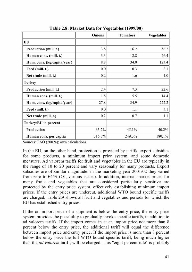
Table 2.8: Market Data for Vegetables (1999/00) Onions Tomatoes Vegetables

EU

Production (mill. t.) 3.8 16.2 56.2

Human cons. (mill. t.) 3.3 12.8 46.4

Hum. cons. (kg/capita/year) 8.8 34.0 123.4

Feed (mill. t.) 0.0 0.3 2.1

Net trade (mill. t.) 0.2 1.6 1.0

Turkey

Production (mill. t.) 2.4 7.3 22.6

Human cons. (mill. t.) 1.8 5.5 14.4

Hum. cons. (kg/capita/year) 27.8 84.9 222.2

Feed (mill. t.) 0.0 1.1 3.1

Net trade (mill. t.) 0.2 0.7 1.1

Turkey/EU in percent

Production 63.2% 45.1% 40.2%

Human cons. per captia 316.5% 249.3% 180.1%Sources: FAO (2002a); own calculations.

In the EU, on the other hand, protection is provided by tariffs, export subsidies for some products, a minimum import price system, and some domestic measures. Ad valorem tariffs for fruit and vegetables in the EU are typically in the range of 10 to 20 percent and vary seasonally for many products. Export subsidies are of similar magnitude: in the marketing year 2001/02 they varied from zero to €45/t (OJ, various issues). In addition, internal market prices for many fruits and vegetables that are considered particularly sensitive are protected by the entry price system, effectively establishing minimum import prices. If the entry prices are undercut, additional WTO bound specific tariffs are charged. Table 2.9 shows all fruit and vegetables and periods for which the EU has established entry prices.

If the cif import price of a shipment is below the entry price, the entry price system provides the possibility to gradually invoke specific tariffs, in addition to ad valorem tariffs. If the import comes in at an import price not more than 8 percent below the entry price, the additional tariff will equal the difference between import price and entry price. If the import price is more than 8 percent below the entry price the full WTO bound specific tariff, being much higher than the ad valorem tariff, will be charged. This "eight percent rule" is probably

42

a prohibitive import barrier for most imports below 92 percent of the entry price, because of the high level of the maximum specific tariffs.7

From an economic point of view, a minimum import price system implemented like the entry price system of the EU could be compared to a voluntary export restraint. In the case of the minimum import price system, the minimum import price implicitly defines a maximum import quantity. In the case of a voluntary export restraint, the import quantity agreed upon implicitly defines the market price in the importing country. In both cases an economic rent results from the export price being higher than the marginal costs of the exporting country.

Table 2.9: Fruit and Vegetables Covered by the EU Entry Price System

Product Time period

Vegetables Artichokes

Courgettes

Cucumbers

Tomatoes

1 November – 30 June

All year

All year

All year

Fruit Sweet oranges

Clementines, Mandarins, Satsumas

Lemons

Apples

Pears

Apricots

Cherries

Peaches, Nectarines, Plums

Table grapes

1 December – 31 May

1 November – end February

1 June – 31 May

All year

1 July – 30 April

1 June – 31 July

21 May – 10 August

11 June – 30 September

21 July – 20 November Source: Agra Europe (London) Ltd. (2003).

It is difficult to assess the restrictiveness of the entry price system for Turkish fruit and vegetable exports to the EU. Should Turkish farmgate prices be considerably below EU farmgate prices, one would expect the entry price system to be restrictive. As a first step, therefore, farmgate prices for selected entry price products are compared between the EU and Turkey in Table 2.10 for 1990 and the period 1995 to 2001.

7 For a detailed overview of the entry price system and its effects see Grethe and Tangermann (1999b).

43

Table 2.10: Turkish and EU Prices for Fruit and Vegetables Covered by the EU Entry Price System (€/t)

1990 1995 1996 1997 1998 1999 2000 2001Table Tomatoes Spanish price 400 285 306 446 485 469 641 495 Greek price 344 591 730 778 692 702 789 830 Turkish price 302 171 260 255 245 211 246 n.a. Turk. price in % of S/G av. 81% 39% 50% 42% 42% 36% 34% Cucumbers Spanish price 439 382 428 359 348 401 396 553 Greek price 488 654 704 751 810 735 839 878 Turkish price 275 214 223 289 334 304 296 n.a. Turk. price in % of S/G av. 59% 41% 39% 52% 58% 53% 48% Table Grapes Spanish price 505 527 390 575 485 456 437 455 Greek price 675 763 831 902 952 875 782 975 Turkish price 352 333 323 298 416 420 440 n.a. Turk. price in % of S/G av. 60% 52% 53% 40% 58% 63% 72% Apples Spanish price 420 265 237 275 326 336 255 293 Greek price 293 413 356 402 415 468 442 553 Turkish price 227 293 258 264 314 334 389 n.a. Turk. price in % of S/G av. 64% 87% 87% 78% 85% 83% 112% Oranges Spanish price 187 229 265 215 178 203 155 199 Greek price 268 299 313 247 251 257 279 343 Turkish price 227 256 273 238 223 255 272 n.a. Turk. price in % of S/G av. 100% 97% 94% 103% 104% 111% 125% Lemons Spanish price 178 371 409 273 217 292 232 237 Greek price 367 463 507 445 409 415 439 420 Turkish price 226 352 407 378 461 420 472 n.a. Turk. price in % of S/G av. 83% 84% 89% 105% 147% 119% 141% Mandarins Spanish price 170 290 338 264 274 267 300 285 Greek price 263 297 311 310 277 279 309 342 Turkish price 272 260 261 254 279 273 283 n.a. Turk. price in % of S/G av. 126% 88% 80% 89% 101% 100% 93%

n.a.: Not available. Sources: SIS (various issues), Agricultural Structure; European Communities (2002); own calculations.

44

Table 2.10 shows that farmgate prices for tomatoes, cucumbers, and table grapes were significantly below the average farmgate prices of Spain and Turkey in the period covered. The comparison of farmgate prices for fruit and vegetables across countries, however, seems to be of little explanatory power with respect to political market barriers; even in a completely free trade situation within the EU, farmgate prices among countries differ greatly due to quality differences and transportation costs. For example, the cucumber price in Greece in the year 2000 was more than twice as high as in Spain. For apples and citrus fruit, Turkish and EU farmgate prices were roughly aligned in the period covered, but with significant deviations in some years, especially in the case of lemons.

Although Turkish farmgate prices are significantly below EU levels for some products in some years, the Turkish Undersecretariat of Foreign Trade reports that exporters of fruit and vegetables have no problems with EU entry price levels because domestic prices in Turkey have been higher than entry prices in recent years. This is because considerable marketing costs must be added to the farmgate prices in order to equal cif EU prices. In addition, only the more highly priced share of Turkey's production is eligible to enter the EU market due to quality issues. Traders confirm that on average, farmgate prices are at 40 percent (e.g. tomatoes) to 85 percent (e.g. potatoes) of fob Turkey prices, and quality and transportation cost differences could therefore explain existing price differences at farm level.

The preliminary conclusion drawn from traders’ anecdotes and price comparison is that Turkey's advantage from abolishing the entry price system in the event of a CU would be small. A more detailed analysis of this topic should include the comparison of Turkey's fob export prices to third countries with EU entry prices on a monthly basis.

EU policies for fresh fruit and vegetables, other than price support, are limited to direct aid for producer organizations. In addition, some direct payments are granted for processing activities. For example, tomato paste producers get a subsidy of €313.6/t of tomatoes processed and producers of dried grapes get a direct payment varying from €880 and €3290/ha.8

Olive oil and olives are protected by high tariffs and export subsidies in the EU (in the marketing year 2001/02, however, no export subsidies were granted). In addition, producers receive direct premiums of €1322.5/t of olive oil (or the table olive equivalent). Also Turkey applies tariffs to imports of olives and olive oil, and export subsidies to olive oil. In order to evaluate the effect of price-

8 EC Reg. 1441/2002 in OJ L212, 08.08.2002.

45

supporting policies on olive oil and olives, EU and Turkish prices are compared in Table 2.11.

Table 2.11: Prices for Olives and Olive Oil in Turkey and the EU (€/t) 1990 1995 1996 1997 1998 1999 2000 2001Olives Spanish price 376 746 767 422 560 613 596 498 Greek price 908 1,051 1,154 1,246 1,145 1,146 1,247 1,324 Turkish price 798 694 748 656 687 886 883 n.a. Turk. price in % of S/G av. 124% 77% 78% 79% 81% 101% 96%

Olive oil Spanish price n.a. 2,706 3,555 2,367 1,804 2,234 1,830 1,639 Greek price 3,017 2,660 3,663 2,824 2,187 2,242 2,172 2,187 Turkish price 4,315 3,128 2,485 3,025 3,931 n.a. Turk. price in % of S/G av. 120% 121% 125% 135% 196% n.a.: Not available. Sources: SIS (various issues), Wholesale Price Statistics; SIS (various issues), Agricultural Structure; European Communities (2002); own calculations.

Table 2.11 shows that EU farmgate prices for olives were extremely heterogeneous during the period covered. In most of the years covered, Greek prices were more than twice as high as those in Spain. Turkish prices were somewhere between the Greek and the Spanish price in most of the years. Olive oil prices in Turkey were above Greek as well as the Spanish levels from 1996 to 2000. This is somewhat surprising as Turkey was a net exporter in all those years and Turkish export subsidies were low (between €3.5 and €200/t in the period covered), so subsidies cannot explain the difference. One possible explanation could be the stage of price collection: EU prices are selling prices of olive oil producers and Turkish prices are wholesale prices. Depending on market structure, prices could, for example, cover different package sizes.

2.2.4 Meat

Table 2.12 presents market surveys for the average of the years 1999 and 2000 in the EU and Turkey for meat. The EU is a significant net exporter of bovine and poultry meat as well as total meat, but a net importer of sheep and goat meat. Turkey does not export or import significant quantities of meat. Turkish meat consumption per head is about 22 percent of the EU level, which is explained by the tremendous difference in income. Only for sheep meat does Turkish per capita consumption exceed that of the EU.

46

Table 2.12: Market Data for Meat (1999/00) Bovine

meat Sheep and goat meat

Poultry Total meat

EU

Production (mill. t.) 7.55 1.13 8.71 36.23

Human cons. (mill. t.) 7.19 1.30 7.80 34.22

Hum. cons. (kg/capita/year) 19.12 3.46 20.74 91.01

Net trade (mill. t.) 0.38 -0.23 0.80 2.03

Turkey

Production (mill. t.) 0.37 0.37 0.56 1.31

Human cons. (mill. t.) 0.37 0.37 0.56 1.31

Hum. cons. (kg/capita/year) 5.71 5.71 8.64 20.22

Net trade (mill. t.) 0.00 0.00 0.00 0.00

Turkey/EU in percent

Production 4.9% 32.7% 6.4% 3.6%

Human cons. per capita 29.9% 165.1% 41.7% 22.2%Sources: FAO (2002a); own calculations.

In Turkey, meat markets are protected by prohibitive tariffs. In addition, Turkey has introduced an import ban on red meat and live animal imports due to the danger of a potential outbreak of foot and mouth disease in August 1996, which was partially lifted for breeding cattle in August 1999, but remains in force for meat and feeder and slaughter animals. Most observers assume this ban to be primarily motivated by protectionist aims (USDA, various issues). The EU markets for meat are protected by tariffs and export subsidies (except for sheep meat). Tariffs for poultry meat are around 35 percent ad valorem equivalent and tariffs for red meat are above 100 percent ad valorem equivalent. The intervention price system for bovine meat was abolished and was replaced in July 2002 by a system of private storage aid, which can be paid if market prices fall below 103 percent of the basic price (€2,224/t). In order to display the effects of market price support on domestic prices, EU and Turkish meat prices are compared in Table 2.13.

47

Table 2.13: Meat Prices in Turkey and the EU (€/t) 1990 1995 1996 1997 1998 1999 2000 2001

Bovine meat

EU price 2,734 2,671 2,291 2,374 2,400 2,256 2,324 2,045

Turkish price 2,312 3,003 2,419 2,838 3,716 3,820 3,729 2,437

Turkish price in % of EU 85% 112% 106% 120% 155% 169% 160% 119%

Sheep meat

EU price 3,416 3,138 3,629 3,757 3,260 3,300 3,573 4,115

Turkish price 2,335 3,325 3,070 3,152 3,196 3,650 3,886 2,444

Turkish price in % of EU 68% 106% 85% 84% 98% 111% 109% 59%

Poultry

EU price 1,163 992 1,090 1,073 1,007 911 977 1,040

Turkish price 1,374 1,332 1,172 1,212 1,526 1,387 1,296 1,023

Turkish price in % of EU 118% 134% 108% 113% 152% 152% 133% 98%Sources: OECD (2002a); own calculations.

Prices for bovine meat in Turkey were close to the EU level until 1996 and greatly exceeded EU prices since. This is due to increasing Turkish prices on the one hand, and decreasing EU prices on the other. For sheep meat, the EU price was relatively stable around €3,500/t from 1990 to 2001 and the Turkish price was around the same level with a sharp drop in 2001. Also for poultry meat, the EU price level was relatively stable since 1990 at a level of €1000/t. The Turkish poultry meat price was about 10 to 50 percent above the EU level in that period with a sharp drop to the EU level in 2001. The significant price drop for all meats in 2001 expressed in € is to be interpreted against the background of a strong devaluation of the Turkish Lira during the Turkish financial crisis.

Both, sheep meat and beef producers in the EU receive several kinds of direct income payments which are coupled to actual numbers of animals kept. In the case of cattle, these premiums added up to about €3.8 billion in 1999, which is roughly equivalent to about 20 percent of the domestic market value of beef, or €500/t. In the case of sheep and goat meat, premiums added up to €1.9 billion in 1999, equivalent to about 46 percent of domestic market value or €1660/t.

In a CU, Turkish prices for poultry and bovine meat are expected to fall to the EU level and Turkey would become a net importer for these products. For sheep meat, the effect is expected to be of little significance as in recent years prices have been quite similar in Turkey and the EU.

48

Considering the very low consumption level of meat in Turkey currently, and the expected income growth and high income elasticities for meat (see Section 6.3.2), meat demand in Turkey is expected to rise significantly. In order to analyze the effects of a CU with the EU, the potential of the Turkish meat industry to keep pace with this demand development is of crucial importance. Poultry meat production is a more or less industrial production technology that can be expanded based on imported feed. Red meat production, however, is based on coarse feed, which competes for land with alternative uses.9 In order to look at the Turkish production potential for red meat, Graph 2.1 presents the development of ruminant animal herds from 1960 to 2002.

Graph 2.1: Ruminants in Turkey (1960-2002)

Sources: FAO (2002a); own calculations.

Graph 2.1 shows that cattle herds have declined by 35 percent and aggregated sheep and goat herds have declined by 50 percent compared to the early eighties. This decline can partially be explained by political and socioeconomic problems in the southeastern part of Turkey (USDA, GAIN Report TU 1034, 21.08.2001, p. 2), and is therefore potentially reversible.

9 Coarse feed is used throughout this study to comprise feed from pasture as well as feed crops.

0

10

20

30

40

50

60

1960 1970 1980 1990 2000

Year

Mill

ion

anim

als

CattleGoatsSheep

49

2.2.5 Eggs and Milk

Table 2.14 presents market surveys for the average of the years 1999 and 2000 in the EU and Turkey for eggs and dairy products.

Table 2.14: Market Data for Eggs and Dairy (1999/00) Eggs Milk equivalent

EU

Production (mill. t.) 5.32 126.25

Human consumption (mill. t.) 4.71 107.91

Human consumption (kg/capita/year) 12.53 286.99

Feed (mill. t.) 0.00 7.12

Net trade (mill. t.) 0.14 9.93

Turkey

Production (mill. t.) 0.69 9.84

Human consumption (mill. t.) 0.61 9.54

Human consumption (kg/capita/year) 9.41 147.22

Feed (mill. t.) 0.00 n.a.

Net trade (mill. t.) 0.01 -0.09

Turkey/EU in percent

Production 13.0% 7.8%

Human consumption per capita 75.1% 51.3% n.a.: Not available. Sources: FAO (2002a); own calculations.

The EU is a net exporter of eggs and dairy products whereas Turkey is a net importer of dairy products and has a trade balance for eggs close to zero. Human consumption per capita in the EU is higher than in Turkey, but the difference is not as distinct as for meat.

In the EU, eggs and dairy products are protected by tariffs with an ad valorem equivalent of about 50 percent for eggs and between 30 and 110 percent for various dairy products. Export subsidies and an intervention price system for butter and skim milk powder (SMP), together with a supply control system, add to the protection granted through tariffs. Under the intervention price system, prices for SMP and butter are fixed at €2,055/t and €3,282/t, respectively. These prices, after deduction of a processing margin, result in a milk target price of €310/t. As unrestricted farm supply in the EU would exceed domestic demand

50

much more than it currently does at this price, production quotas are allocated to member states and individual farmers in order to limit budgetary costs and comply with WTO commitments regarding export subsidies. Under the Agenda 2000 reform package, intervention prices are to be reduced by 15 percent in three annual steps from 2005 on, and compensatory payments of a final yearly amount of €17.24/t are foreseen. Further reform of the dairy market in the EU is currently under discussion.

In Turkey, dairy and egg prices are protected by high tariffs (between 67 and 150 percent for dairy products and 54.2 percent for eggs in 2002) and relatively low export subsidies.

In order to depict the effects of various price policies on market prices in the EU and Turkey, Table 2.15 compares prices for eggs, milk, butter, and SMP for 1990 and from 1995 to 2001. For eggs, the farmgate price in Turkey was significantly above the EU level from 1995 to 2001. For cows milk, on the other hand, the Turkish farmgate price was 10 to 30 percent below the EU level from 1990 to 2001, with the exemption of the years 1997 and 1998 in which Turkish prices were close to EU levels. In the event of market integration between Turkey and the EU, however, competition would not take place at the level of raw milk but rather for processed products like cheese, butter, and SMP. Therefore the prices of SMP and butter are compared, too, as these are, in contrast to cheese, relatively homogeneous products. For this comparison, the EU prices are the intervention prices and for Turkey, butter prices are from the SIS Wholesale Price Statistics. As no official SMP price data exists, prices are selling prices of two private dairy companies in Turkey. Prices for butter and SMP in Turkey exceeded those in the EU, sometimes by more than 100 percent in the years 1996 to 2000. If a synthetic milk price is calculated by weighting butter and SMP prices with their respective extraction shares, the Turkish price in recent years was about twice the EU price, while the milk price received by the farmer was lower. Various reasons could contribute to such high processing margins in Turkey: i) due to the low number of cows per farmer the cost of milk collection is higher than in the EU, ii) due to the low number of cows per household a considerable share of milk fat remains at the farm resulting in a low fat content of the milk delivered to the factory, iii) higher processing cost due to less developed technology, or iv) higher profit margins in the milk processing industry. Profit margins exceeding usual rates for paying entrepreneurs for their risk and production factors can only be explained by limited competition, that is some kind of cartel formation. This seems at least possible, as the Turkish market is largely isolated from international competition and the market structure for processed products is oligopolistic (AKSOY, 2000).

51

Table 2.15: Egg and Dairy Prices in Turkey and the EU (€/t) 1990 1995 1996 1997 1998 1999 2000 2001Eggs EU price 1,026 678 818 794 694 641 762 746 Turkish price 958 1,211 1,221 1,233 1,101 1,052 1,469 1,239 Turkish price in % of EU 93% 179% 149% 155% 159% 164% 193% 166%Milk (farmgate) EU price 298 305 309 307 307 294 310 320 Turkish price 225 217 249 312 304 272 289 244 Turkish price in % of EU 76% 71% 81% 102% 99% 92% 93% 76%Butter EU price 3,381 3,282 3,282 3,282 3,282 3,282 3,282 3,282 Turkish price 3,643 4,250 4,281 7,156 7,402 n.a. Turkish price in % of EU 111% 130% 130% 218% 226%SMP EU price 1,991 2,055 2,055 2,055 2,055 2,055 2,055 2,055 Turkish price 2,488 4,490 4,624 3,869 4,407 n.a. Turkish price in % of EU 121% 218% 225% 188% 214%Synthetic milk price EU price 330 331 331 331 331 331 331 331 Turkish price 387 596 609 667 727 Turkish price in % of EU 117% 180% 184% 201% 219%Processing margin EU 32 27 23 24 25 37 22 12 Turkey 138 283 305 395 437 Turkey in % of EU 602% 1182% 1229% 1065% 2021%n.a.: Not available. Sources: OECD (2002a); AgraEurope (London) Ltd. (2003); SIS Wholesale Price Statistics (various issues); skim milk powder prices from private companies; own calculations.

The preliminary conclusion is that in the event of a CU, processed dairy products as well as eggs would be exported from the EU to Turkey due to higher prices in Turkey. For a more detailed analysis it would be important to obtain better price information, particularly for SMP, and to investigate the reasons for higher processing margins in Turkey.

52

2.3 Non-Product-Specific Agricultural Policies

In the past, Turkey has provided a high degree of support to farmers through subsidization of inputs such as fertilizer and credit subsidies. These policies, however, have been phased out (fertilizer subsidies in 2001, credit subsidies in 2000). Subsidies for pesticides and seed, however, were still in place in 2002. Most farmers in Turkey are exempt from income tax payments (OECD 2002b).

In 2001, Turkey started to implement a major World Bank-supported agricultural policy reform program to be completed by 2004 (OECD 2001c, 2002b). Under this program, all credit and input subsidies as well as price support provided through state enterprises and agricultural sales cooperatives (valued before reform at about $5 billion US) are to be replaced by $1.9 billion of direct income payments to farmers. These payments are set at $81/ha and are limited to 20 ha per farmer. A major challenge for the implementation of such a system in a country like Turkey is the registration of farmers and agricultural area and the distribution of cash support; Turkey has about 4 million agricultural holdings (compared to 7 million in the EU) and the system of area registration is much less developed.

In addition to the product-specific policies discussed previously, agriculture in the EU is supported in various other ways. The largest budget share spent on a single policy is allocated to direct payments for cereals and oilseeds, which are no longer product specific since implementation of the Agenda 2000 reform package. These payments consume about 30 percent of the EU budget and are granted per ha grown with cereals, oilseeds, or set aside (up to 30 percent of area eligible for premium). The level of payments per ha is determined according to regional average yield in a base period and is currently at €63/t. Another large share of the EU budget (about 16 percent) is spent for the so-called second pillar of the CAP, which covers various policies summarized under rural development. This policy package includes such heterogeneous measures as agroenviron-mental measures, investment aid, aid for less favoured areas, and early retirement schemes.10 Furthermore, many EU member states provide significant support to the agricultural sector through tax exemptions and budgetary outlays for specific agricultural social security systems.

10 For a detailed overview of the second pillar and an outlook on future developments, see Grethe (2002).

53

3 DEVELOPMENT AND STATUS OF AGRICULTURAL TRADE RELATIONS BETWEEN TURKEY AND THE EUROPEAN UNION

3.1 Overview of Agricultural Trade between Turkey and the European Union

The EU is the most important single trading partner of Turkey in total trade as well as in agricultural trade. Table 3.1 presents an overview of Turkish and EU external trade for the years 1989/90 and 1995 to 2001. Trade data reported is averaged for two calendar years, except single year data for 1995. This is because 1995 is the only pre-CU year of the full EU-15; the CU came into force January 1996. Before 1995, the EU had 12 member states. Therefore trade data for those years is less suitable for depicting a CU effect, as an increase in trade from 1996 on may also be due to the inclusion of the three new member states.

Table 3.1: Trade Overview of Turkey and the EU (bill. €) 1989/90 1995 1996/97 1998/99 2000/01

Turkey Total exports 10.4 16.5 20.8 25.2 32.5

of which to EU 55.4% 46.0% 53.1% 56.9% 58.0%Total imports 15.9 27.3 38.7 40.6 52.6

of which from EU 41.9% 32.5% 52.4% 52.6% 47.6%Agricultural exports 2.5 3.3 4.1 3.8 4.3

of which to EU 38.0% 47.8% 44.1% 51.2% 48.7%Agricultural imports 1.6 2.7 3.3 2.8 3.0

of which from EU 29.0% 30.3% 27.5% 27.6% 25.6% EU Total exports 414.3 569.0 671.8 746.7 959.8

of which to Turkey 1.6% 2.4% 3.0% 2.9% 2.6%Total imports 454.6 544.7 624.8 743.6 1,026.8

of which from Turkey 1.3% 1.7% 1.8% 1.9% 1.8%Agricultural exports 33.7 43.4 48.0 49.0 55.7

of which to Turkey 1.4% 1.9% 1.9% 1.6% 1.4%Agricultural imports 38.6 46.3 49.5 50.2 55.5

of which from Turkey 2.5% 3.4% 3.7% 3.9% 3.7%Sources: SIS, External Trade Statistics (various issues); Eurostat, Intra- and Extra-EU Trade (various issues); FAO (2002a); own calculations.

Table 3.1 shows that Turkey's total exports tripled in the period from 1989/90 to 2000/01 from €10.4 billion to more than €32 billion. Over the entire period

54

Turkey had a trade deficit increasing from €5.5 billion in 1989/90 to more than €20 billion in 2000/01. About 46 to 58 percent of Turkey's total exports went to the EU and 33 to 53 percent of Turkey's total imports came from the EU. As for Turkish imports, where one would expect any effects from the CU in industrial products to be realized in 1996, such effects are not very distinct. On the one hand, the share of EU imports in total Turkish imports increased from about 33 percent in 1995 to more than 52 percent in the period 1996 to 1999. On the other hand, the share of the EU was already at 42 percent in 1989/90 (prior to Austria, Sweden, and Finland becoming EU members) and was only 48 percent in 2000/01.

Turkey has almost doubled its agricultural exports between 1989/90 and 2000/01 from €2.5 to €4.3 billion.11 In all those years, Turkey had an agricultural trade surplus which varied between €0.6 billion in 1995 and €1.3 billion in 2000/01. The share of the EU in total agricultural trade of Turkey varied between 38 and 51 percent of Turkish exports and 26 to 30 percent of Turkish imports. Overall Turkey had a clear surplus in agricultural trade with the EU over the whole period.

The EU has more than doubled its total exports between 1989/90 and 2000/01 from €414 billion in 1989/90 to almost €960 billion in 2000/01. On average the EU had a balanced trade position with a slight export surplus in some years and an import deficit in others. Between 1.6 and 3 percent of EU exports went to Turkey and at the importing side Turkey's share varied between 1.3 and 1.9 percent.

The EU has also increased its agricultural exports and imports during the period presented here, but not as much as total trade. The EU had a declining deficit in agricultural trade between 1989/90 and 1998/99 and, for the first time in the period covered, a slight agricultural trade surplus in 2000/01. About 1.4 to 1.9 percent of EU agricultural exports went to Turkey and at the importing side, Turkey covered a share between 2.5 and 3.9 percent of agricultural imports.

Table 3.2 presents an overview of the composition of total Turkish agricultural imports as well as those originating from the EU.

11 Agricultural trade is defined throughout this chapter to include CN-Chapters 01-24, except Chapter 03 (fish), and CN-positions 41.01-03, 51.01-03, 52.01-03 (hides and skins, wool and cotton).

55

Table 3.2: Composition of Turkish Agricultural Imports by Origin (percent)

1989/90 1995 1996/97 1998/99 2000/01 Total EU Total EU Total EU Total EU Total EU

Meat & live animals 3.8 4.4 11.3 5.9 2.4 6.6 0.8 1.8 1.0 2.5

Dairy and eggs 0.7 1.2 0.9 3.0 0.8 2.5 1.1 3.4 1.0 2.1

Vegetables 1.1 0.4 0.7 0.9 0.9 0.5 1.0 1.2 2.9 0.5

Fruit 0.6 0.5 1.3 0.6 1.4 0.3 2.1 0.6 1.7 0.7

Cereals & cereal. prod. 30.2 33.3 12.7 6.8 18.1 9.5 14.5 10.6 10.8 9.2

Oilseeds 2.1 1.5 6.4 4.7 6.8 2.8 9.4 3.7 7.4 4.3

Fats & oils 16.2 14.3 17.2 11.5 12.6 6.8 14.5 11.4 11.5 7.6

Sugars & confectionery 7.4 19.2 5.4 3.0 3.8 8.1 0.4 1.5 0.4 1.2

Prep. of fruit & veg. 0.1 0.2 0.3 0.5 0.4 0.6 0.7 0.8 0.5 1.0

Beverages & spirits 0.4 4.7 0.4 10.6 0.8 6.1 0.5 6.9 0.5 7.8

Tobacco 14.5 1.8 4.3 4.7 7.9 7.9 9.2 11.0 10.7 8.5

Hides and skins 6.0 6.7 12.5 21.5 14.9 16.8 7.1 10.2 8.5 14.5

Cotton lint 6.2 3.0 10.3 5.9 11.3 12.1 14.6 11.7 19.9 17.5

Other products 10.7 8.7 16.1 20.3 18.0 19.5 24.2 25.3 23.2 22.7

Total 100 100 100 100 100 100 100 100 100 100Sources: SIS External Trade Statistics (various issues); Eurostat Intra- and Extra-EU Trade (various issues); FAO (2002a); own calculations.

In 1989/90, cereals and cereal products, fats and oils, and tobacco were the most important agricultural import products covering more than 60 percent of total Turkish agricultural imports. The composition of imports from the EU was close to the composition of total imports with the main differences being a much lower share of tobacco and a much higher share of beverages and spirits, and sugar and confectionery.

By 2000/01 Turkey's total agricultural imports were more diverse as the share of the product group "other products" increased from 11 to about 23 percent, and the importance of cereals and cereal products as well as fats and oils declined significantly. The import share of cotton increased heavily reflecting the growing Turkish textile industry, which accounts for a large share of Turkish industrial exports. The composition of agricultural imports from the EU was still close to that of total agricultural imports, but shares of beverages and spirits as well as hides and skins were significantly higher than in total agricultural imports.

56

Table 3.3 presents an overview of the composition of total agricultural exports of Turkey as well as those destined for the EU.

Table 3.3: Composition of Turkish Agricultural Exports by Destination (percent)

1989/90 1995 1996/97 1998/99 2000/01 Total EU Total EU Total EU Total EU Total EU

Meat & live animals 8.6 0.3 3.4 0.1 2.0 0.2 1.1 0.1 1.0 0.2

Dairy and eggs 0.6 0.3 0.6 0.2 1.1 0.5 1.2 0.4 0.8 0.3

Vegetables 11.3 11.9 8.6 8.0 7.6 7.6 3.5 5.7 8.2 6.8

Fruit 27.6 41.9 28.0 45.3 24.7 44.5 24.6 44.1 28.5 44.9

Cereals & cereal. prod. 4.8 1.6 10.9 2.1 12.3 1.5 12.2 2.5 10.1 3.5

Oilseeds 1.4 2.7 1.5 2.0 1.0 1.9 1.4 2.0 1.2 1.8

Fats & oils 6.8 0.4 10.7 0.7 7.7 2.7 8.2 3.8 5.0 2.5

Sugars & confectionery 0.6 0.4 4.3 0.5 4.6 0.4 5.1 0.6 7.0 1.0

Prep. of fruit & veg. 10.1 15.4 12.0 20.6 11.9 19.4 14.3 19.8 12.9 18.9

Beverages & spirits 0.4 0.6 2.0 0.7 1.8 0.8 1.2 1.0 0.9 1.2

Tobacco 15.4 6.4 8.6 6.2 13.3 5.7 13.9 6.2 11.8 6.4

Hides and skins 0.0 0.0 0.1 0.1 0.1 0.1 0.4 0.1 0.7 0.1

Cotton lint 5.3 8.4 0.9 3.9 2.5 4.2 2.5 3.4 1.6 2.9

Other products 7.3 9.7 8.6 9.4 9.4 10.6 10.4 10.2 10.1 9.6

Total 100 100 100 100 100 100 100 100 100 100Sources: SIS, External Trade Statistics (various issues); Eurostat, Intra- and Extra-EU Trade (various issues); FAO (2002a); own calculations.

At the end of the eighties, Turkey's most important export products were fruit and vegetables (fresh as well as processed), and tobacco which together covered more than 65 percent of total Turkish agricultural exports. The composition of exports to the EU was quite similar to that of total agricultural exports with the main difference being a significantly lower share of tobacco and higher shares of fruit and processed fruit and vegetables with the result that fruit and vegetables alone covered almost 70 percent of Turkish agricultural exports to the EU.

In 2000/01 the composition of Turkish agricultural exports was only slightly different from that in 1989/90. Main differences were a higher share of cereals and cereal products and lower shares of cotton lint, reflecting increasing domestic processing demand, and meat and live animals, reflecting the import ban on red meat (see Section 2.2.4). The share of fruit and vegetable exports in

57

total agricultural exports to the EU increased slightly compared to the 1989/90 situation, exceeding 70 percent.

3.2 Agricultural Trade Preferences between Turkey and the European Union

Trade preferences in agriculture have been granted by the EU to Turkey since the Association Agreement in 1963 and have been extended several times. Since 1998, Turkey has also established significant preferential market access for the EU. The analysis of current trade preferences is important for the assessment of an extension of the CU to cover agricultural products. This is because such an assessment will mainly be based on price differences between Turkey and the EU and on specific trade policies applied to trade between Turkey and the EU, and not based on most favored nation (MFN) market barriers.12 A CU in agriculture would have direct effects only on those products for which political trade barriers between Turkey and the EU are still in force. In case of products for which significant price differences between the EU and Turkey do exist, in the absence of any tariffs and/or export subsidies or other trade policies there is no reason to assume that these price differences would automatically disappear with a CU.

Section 3.2.1 first describes agricultural trade preferences currently in force for agricultural exports from Turkey to the EU. In Section 3.2.2, preferences applied to agricultural exports of the EU to Turkey are described. Finally, in Section 3.2.3, trade preferences for a very specific group of processed products, known as Non-Annex I products, are analysed.

3.2.1 EU Preferences Granted for Agricultural Products Originating from Turkey

Agricultural products as defined by the EU are products covered by Annex II of the Treaty of Rome. These are farm products as well as most first stage processed products such as wheat flour, olive oil, and fruit juice. Thus most products in CN chapters 1-24 and some products in higher chapters are agricultural products. Since the Association Agreement, at various times tariff preferences have been granted by the EU for agricultural products originating

12 The MFN tariff is the tariff charged on imports from nonpreferred third countries, as far as these third countries are WTO members. In the EU, it is usually the tariff bound in the WTO, i.e. the tariff that must not be exceeded if charged on products originating from WTO members.

58

from Turkey. Since 1987, almost all ad valorem tariffs have been abolished. In some cases reduced rates are also granted for specific duties.13

In order to analyze the extent of current preferences granted to Turkey, agricultural commodities are classified into four groups, depending on the import regime applied by the EU to imports originating from Turkey:14

1. Products for which no MFN import barriers exist (MFN tariff = 0, no entry price).

2. Products with a MFN tariff and/or an entry price and no preferential treatment for imports from Turkey.

3. Products with a MFN tariff and/or an entry price and a partial preference for imports from Turkey (for example, a reduced MFN tariff rate).

4. Products with a MFN tariff and/or an entry price and no import barrier for imports from Turkey (tariff = 0, no entry price applied).

To get an idea of the relative importance of these different product groups, Turkey's 2001 agricultural exports to the EU are classified according to these groups and displayed in Table 3.4. About seven percent of Turkey's agricultural exports of the year 2001 are in group 1 and preferential treatment is technically impossible because MFN market barriers do not exist. This group consists mainly of products of CN-chapter 5 (particularly entrails and organs), CN-chapter 12 products (oilseeds and oleaginous fruit), and some vegetables. Only about two percent of Turkey's agricultural exports to the EU are in group 2 and were subject to a tariff at MFN conditions in 2001(and, in some cases, a minimum import price). Fruit and vegetables account for more than 80 percent of this group, consisting mainly of grapes, for which no preferences are granted in certain periods of the year. About 91 percent of agricultural exports are in groups 3 (36 percent) and 4 (54 percent) and were exported to the EU in 2001 under preferential conditions. Group 3 mainly consists of fruit subject to MFN minimum import prices but not to the MFN ad valorem duty. The most important products in group 4 are fruit (CN-chapter 8, about 48 percent of group

13 Specific duties in the EU mainly apply to meat, dairy products, sugar, and cereals, i.e. products that were protected by variable levies before implementation of the Uruguay Round Agreement.

14 A detailed overview of existing preferences (state of April 2001) for agricultural products is given in the Annex to Chapter 3. Information in the Annex is extracted from the TARIC (OJ C119A, 23.04.2001) and crosschecked with Decision No. 1/98 of the Association Council (OJ L 86, 20.03.1998).

59

4), preparations of fruit and vegetables (CN-chapter 20, about 20 percent of group 4) and vegetables (CN chapter 7, about 7 percent of group 4).

Table 3.4: Classification of Turkish Agricultural Exports to the EU According to the EU's Import Regime, 2001 (€1,000)

Product group Group 1 No MFN barrier

Group 2 MFN

barrier, no pref.

Group 3 MFN

barrier, partial pref.

Group 4 MFN

barrier, Turkey free

Total

€1,000 % €1,000 % €1,000 % €1,000 % €1,000 % Live animals 3,232 99 0 1 0 31 1 3,263 100Meat 0 52 5 38 3 1,003 92 1,093 100Dairy, eggs... 0 0 0 5,721 100 5,721 100Other an. prod. 37,812 100 0 0 4 0 37,816 100Plants + flowers 928 6 0 0 14,009 94 14,937 100Vegetables 22,847 15 5,333 3 16,390 11 111,125 71 155,695 100Fruit and nuts 804 0 30,246 3 595,453 59 379,804 38 1,006,306 100Coffee, tea 10,364 55 0 0 8,596 45 18,960 100Cereals 9,318 21 1,020 2 33,099 76 0 43,437 100Cereal prod. 0 769 6 0 11,762 94 12,531 100Oilseeds... 38,021 91 0 0 3,882 9 41,903 100Lacs, gums... 182 99 0 0 1 1 183 100Plaiting mat. 13,229 100 0 0 0 13,229 100Fats + oils 815 1 0 73,823 87 10,334 12 84,972 100Meat + fish prep. 37 0 10 0 0 20,230 100 20,277 100Sugar + confect. 0 2,623 11 12,255 53 8,432 36 23,310 100Cocoa + prep. 0 0 2,004 14 12,374 86 14,378 100Prep. of cereals 0 0 20,996 100 4 0 21,000 100Veg. + fruit prep. 6 0 2,499 1 12,054 3 401,966 97 416,525 100Other prep. 0 6 0 3,783 21 14,045 79 17,834 100Bever. + spirits 12,712 46 14 0 49 0 14,724 54 27,499 100Resid., fodder 279 18 1,260 80 0 40 3 1,579 100Tobacco 0 0 0 133,184 100 133,184 100Total (in mill. €) 151 7 44 2 770 36 1,151 54 2,116 100Sources: TARIC (OJ C 119 A, 23.04.2001); EUROSTAT Intra- and Extra-EU Trade (various issues); own calculations.

Summarizing all this, it seems that Turkey's exports to the EU are subject to a relatively liberal regime. More than 60 percent (in terms of import value) enter the EU market tariff free and without any other restrictive border measure

60

(groups 1 and 4). Slightly more than 90 percent (groups 3 and 4) are subject to preferential conditions.

However, these calculations do not fully reflect the protective effect of the current import barriers of the EU. It remains an open question as to how Turkey's exports to the EU would fare in the absence of any tariffs and entry prices. Even if most of the products which enter the EU market do so under preferential conditions, many product groups in the EU are still protected by prohibitive tariffs. The removal of these tariffs could result in increased exports from Turkey to the EU, and of course, such potential exports are not included in these calculations.

To get a picture of the currently remaining EU trade barriers for imports originating from Turkey, the following list provides an overview of these measures and their significance.

• High, specific duties apply for almost all imports of core products of the CAP like cereals and cereal products, sugar and sugar products, dairy, meat, live animals, and for some other products of importance for Turkey like olive oil.

• Specific duties apply to EU imports of a lot of processed agricultural products e.g. cereal preparations (CN-chapter 19) and preparations of fruit and vegetables (CN-chapter 20).

• The entry price system for eleven different kinds of fruit, four vegetables, and grape juice and must (the entry price system is described and its impact is discussed in Section 2.2.3 above) fully applies to EU imports originating from Turkey.

• Calendar restrictions apply to preferential tariffs for four different kinds of fruit and nine vegetables. EU imports of most fruit and vegetables originating from Turkey are tariff free (if the entry price is respected). For some of these products, however, this suspension of the MFN tariff is limited to certain calendar periods. Table 3.5 provides an overview of these products.

61

Table 3.5: Fruits and Vegetables Subject to a Seasonal ad valorem Tariff

Product Calendar period Tariff applied (2001)

Potatoes

Onions

Beans (V. and Ph.) Beans (Vicia F.) Eggplant

Courgettes

Celery

Pumpkins

Wild onions

1. April - 30. June

16. May - 31. December

15. May - 31. October

1. May - 30. June

1 - 14. January, 1. May - 31. December

1-31. December, 1. January -28. February

1. May - 31. December

1. March - 30. November

16. May - 31. December

9.6–13.4 %

9.6 %

10.4 – 13.6 %

11.2%

9.0 – 15.5 %

12.8 %

12.8 %

12.8 %

12.8%

Grapes

Watermelons

Melons

Plums

1. May - 17. June, 1. August - 14. November 1. January - 31. March, 16. June - 31. December 1. June - 31. October

16. June - 31. December

15.8 – 19.4 %

8.8%

8.8 %

7.5 – 14.0 %

and entry price system

and entry price system

Source: TARIC (OJ C 119 A, 23.04.2001).

The remaining ad valorem tariffs are generally in the range of 10 to 20 percent and are limited to relatively few products. Turkey exports relevant quantities of some of these products, for example onions and grapes, to the EU and therefore loses considerable export revenue by paying tariffs.

• Some tariff rate quotas (TRQs), at zero or reduced rates, exist for EU imports originating from Turkey with the full MFN tariff or the specific tariff component only applied for above-quota imports. These TRQs are listed in Table 3.6.

62

Table 3.6: TRQ for Turkish Exports to the EU, Utilisation of TRQ and Tariff Rates

CN code Product TRQ size (tons)

Average 1998-2001 exports to EU (tons)

In-quota tariff

Above-quota tariff

ex 0204 Sheep & goat meat 200 4 0 €1,730/t

ex 0207 Turkey meat 1,000 0 €93-339/t €187-679/t

ex 040690 Selected cheese 1,500 6 0 €672/t

ex 070310 Onions (16.5 - 14.2) 2,000 1,777 0 9.6%

ex 070930 Eggplant (1.5 - 14.1) 1,000 2,649 0 9.5-15.5%

ex 070990 Courgettes (1.3 - 30.11)

500 1,485 0 12.8%

ex 080711 Watermelon (16.6 - 31.3)

14,000 6,054 0 8.8%

ex 0811 Frozen berries 100 11 0 €84/t

ex 2002 Prepared tomatoes 8,000 6,246 0 14.4%

ex 200290 Tomato paste 30,000 26,609 0 14.4%

20079130 Selected fruit prep. 200 24 0 €42-230/t

ex 200850 Apricot pulp 600 no data 0 13.6-17.0%

ex 1902 Pasta €2.5 mill. €1.7 mill. €106.7/t €246/tSources: TARIC (OJ C 119 A, 23.04.2001); EC Reg. 2591/2001 (OJ L 345, 29.12.2001), Decision No. 1/98 of the Association Council (OJ L 86, 20.03.1998); Eurostat Intra- and Extra-EU Trade (supplement 09-10/2002); own calculations.

Table 3.6 shows that the TRQ for eggplant and courgettes were fully utilized and, on average, exceeded from 1998 to 2001 by Turkish exports indicating that above-quota tariffs were an effective barrier to trade and Turkey would gain from an abolition of tariffs. Other TRQs at a zero tariff rate, however, were not fully utilized, e.g. sheep and goat meat, onions, watermelons, frozen berries, prepared tomatoes, tomato paste and selected fruit preparations. This indicates that Turkey would not be able to gain from a total tariff abolition as it does not have the export potential to make use of it, at least in some years. In the case of the in-quota tariff being positive and no exports taking place (turkey meat), nothing can be said a priori about the effect of a total tariff abolition as it is unknown whether any exports would take place in a situation without tariffs. In the case of pasta, where considerable exports take place at the reduced but still high in-quota tariff, it can be assumed that the tariffs, in- and above-quota, have a trade-restricting effect.

63

3.2.2 Turkish Preferences Granted for Agricultural Products Originating from the EU

Traditionally, Turkey has only granted preferences of minor significance for agricultural imports from the EU. After establishment of the CU, however, negotiations of extension of Turkish preferences to cover EU agricultural products were intensified and 39 TRQs for a high variety of products entered into force in January 1998. Table 3.7 shows TRQ larger than 1,000 t, the in- and above-quota tariffs and the actual EU exports to Turkey in 2001.

For many products (butter, other live plants, seed potatoes, rye, cotton seed, animal fats, soya and rapeseed oil, and animal feed) the EU was fully utilizing its zero-tariff TRQ, even exceeding them in 1998-2000, indicating that above-quota tariffs are restricting actual trade. For all other products, EU exports stayed below the TRQ level. Reasons for this are manifold. In the case of meat, the reason simply is the Turkish import ban (see Section 2.2.4) which also applies to imports from the EU. For some products, like prepared tomatoes, the reason may be a sufficient Turkish domestic supply at competitive prices. But, for SMP and wheat, price analysis in Chapter 2 showed Turkish prices significantly exceeding EU prices. It is unclear why, in such a situation, the EU was not able to make full use of its TRQ.

64

Table 3.7: Selected TRQs for EU Exports to Turkey, Quota Utilization and Tariffs

CN code Product TRQ (tons)

EU exports to Turkey (tons, av.

1998-2001)

In-quota tariff

Above-quota tariff

ex 010290 Live cattle 3,500 0 0-69% 138%

020220 Beef 19,000 21 30-43% 230%

040210 Milk powder 4,000 2,368 0 150%

ex 0405 Butter 3,000 3,369 0 100%

040690 Other cheese 2,000 344 0 44-111%

ex 060290 Other live plants 3,000 15,042 0 2.5-20.6%

070110 Seed potatoes 5,000 10,580 0 20.4%

ex 100110 Durum wheat (01.09-31.5) 100,000 4,905 0 5%a

ex 100190 Common wheat (01.09-31.5) 200,000 174,688 0 10%a

ex 1002 Rye (01.9-31.5) 20,000 41,547 0 60%

ex 1003 Barley (01.9-31.5) 46,000 45,010 0 85%

ex 100590 Maize (01.12-31.5) 52,000 11,621 0 10%

100630 Rice 28,000 21,055 0 35%

12072090 Cotton seed 1,500 45,430 0 4%

1502 Animal fats 3,000 5,692 0 4%

ex 150710 Unref. soya oil (1.1-31.8) 60,000 84,969 0 12%

ex 150790 Refined soya oil (1.1-31.8) 2,000 2,887 0 20.6-23%

ex 151211 Raw sunflower oil (1.1-31.8) 18,000 5,333 0 12%

ex 151410 Raw rapeseed oil (1.1-31.8) 10,000 10,890 0 12%

170199 Refined sugar 80,000 12,170 50% 138%

200290 Prepared tomatoes 1,500 183 0 138.9%

2209 Vinegar 2,500 917 0 41.2%

230990 Animal feed 6,000 16,020 0 0-8.2% a Tariffs for wheat do not fully reflect the degree of market protection as Turkey has issued no import licenses for MFN wheat imports since November 1999 (USDA, GAIN Report TU 2014 of 20.03.2002, p. 5).

Sources: Decision No. 1/98 of the Association Council (OJ L 86, 20.03.1998); Eurostat (various issues) Intra- and Extra-EU Trade (supplement 09-10/2002); Undersecretariat of Foreign Trade (various issues), 2002 Tariff Schedule; own calculations.

65

Turkey grants very few preferences for agricultural imports originating from the EU without a TRQ limit. Most of these preferences are relatively insignificant (MFN tariff reductions of 2 percentage points or less). Those products out of CN-chapters 1 to 24 which can be imported from the EU under preferential conditions which are more favorable than a tariff reduction of 2 percentage points and without TRQ restriction are listed in Table 3.8 (non-Annex I products, Table-2 products, and industrial products included in these chapters are discussed in the next section).

Table 3.8: Preferences Granted by Turkey for Agricultural Imports Originating from the EU, 2002

CN code Product Tariff reduction (in percentage points)

130220 Pectic substances, pectinates, pectates 5

2204 Wine from fresh grapes 13.5-20

2206 Cider, perry, mead, other fermented beverages 20

2208 Ethyl alcohol, <80 % spirits 20 Source: Undersecretariat of Foreign Trade (various issues), 2002 Tariff Schedule.

3.2.3 Preferential Trade Arrangements for Non-Annex I Products

Some highly processed products, not covered by Annex II of the Treaty of Rome, are covered by a special import regime for processed agricultural products. Previously these products were widely known as "non-Annex II products." With the adoption of the Treaty of Amsterdam in May 1999, and the resulting changes in some of the EU legal texts, these products are now officially "non-Annex I products."15 Import tariffs for these products reflect, in addition to the protection granted to the processing industry, protection for the incorporated raw agricultural products. Non-Annex I products are protected by a fixed industrial component of the tariff, and an agricultural component that is charged based on the agricultural tariffs charged on certain basic products. For this purpose, basic products are dairy products, cereals, and sugar. There are some problems, however, with this approach. In the case of cereal products, the agricultural component no longer reflects the protection granted for the basic product properly since the implementation of the Uruguay Round Agreement.

15 Those listed in Table 1 of Annex B of EC regulation No 3448/93 (OJ L 318, 20.12.1993) of December 6, 1993 and in Annex 1 of the Customs Union agreement between Turkey and the EU. The term "Non-Annex II products" is used throughout this study for the products contained in Table 1 of Annex B of EC regulation No 3448/93 and not for those contained in Table 2 of this regulation.

66

Due to the way the EU has tarified its former variable levies charged on imports of cereals, the agricultural component charged on processed cereal products (CN-Chapter 19) has increased after implementation of the Uruguay Round Agreement. The agricultural component charged on pasta increased from an average of €33.5/t in 1994/95 to €362/t in 1996 (in a situation of a minimal tariff charged on the basic product due to high world market prices). The industrial component was then reduced in accordance with the WTO rules and is currently at a level of €246/t. This high tariff is practically prohibitive for Turkey's pasta exports to the EU and the EU has granted a preferential rate for Turkey of €106.7/t within a TRQ of €2.5 mill.16 This is still three times higher as before the implementation of the Uruguay Round Agreement. Thus, the non-Annex I system is abused to provide industrial protection via the agricultural component in contradiction with the basic idea of the non-Annex I regime, which is to only compensate for the disadvantage of domestic producers resulting from high domestic prices of basic products.

The industrial component of the tariffs of non-Annex 1 products is included in the CU, i.e. the industrial tariff component does not apply to trade between the EU and Turkey. Further, the agricultural component charged on trade of these products is also exempted from the CU. If preferences are granted for basic agricultural products, these preferences must be taken into account if an agricultural component applies to trade of non-Annex I products between Turkey and the EU.

A second group of processed agricultural products, those contained in Table 2 of Annex B of EC regulation No 3448/93 (referred to as Table-2 products in this study), is not explicitly mentioned in the Customs Union Decision. These products are considered as being industrial products and are therefore fully included in the CU.

The inclusion of the industrial component of non-Annex I and Table-2 products in the CU is often discussed as establishing free trade for processed agricultural products. The real changes are, however, less far reaching. Most processed agricultural products are agricultural products covered by Annex II of the Treaty of Rome, e.g. all preparations of meat and fish (CN-chapter 16), and most fruit and vegetable preparations (CN-chapter 20). These products are therefore not included in the CU.

In order to assess the impact of the changing trade regime on trade flows, trade of non-Annex I and Table-2 products between Turkey and the EU is displayed

16 This TRQ is renewed annually, for 2003 see EC Reg. 2362/2002, OJ L 345, 29.12.2001.

67

in Table 3.9 for the years 1994 to 2000, covering the switch to the CU for industrial products in 1996.

Table 3.9: Trade of Table-2 and Non-Annex I Products between Turkey and the EU (mill. €)

1994 1995 1996 1997 1998 1999 2000

Table 2 products

Turkish exports to the EU 11.3 8.5 15.2 19.9 24.4 16.8 39.2

Turkish imports from the EU 65.9 108.4 176.2 256.1 260.7 75.3 177.8

Non-Annex 1 Products

Turkish exports to the EU 16.4 16.0 17.2 20.3 23.6 23.8 38.6

Turkish imports from the EU 23.2 31.8 48.1 68.6 77.9 45.5 27.9Sources: Eurostat (various issues), Intra- and Extra-EU Trade; own calculations.

Turkish exports of Table-2 products to the EU are volatile and have increased since the mid-nineties, which cannot be due to the implementation of the CU as market access for Table-2 products was free even before 1996.

Turkish imports of Table-2 products from the EU are also very volatile, but have increased considerably since the mid-nineties. This effect could partly be due to the abolition of tariffs under the CU. For all Table-2 products, the EU paid the MFN tariff before the CU. These tariffs are now completely abolished. A much-discussed example among these products are cigarettes (USDA, Gain Report No. TU6024, 05.03.1996). With implementation of the CU, cigarette imports from the EU became tariff free. This development puts a disadvantage on Turkey's domestic cigarette manufacturers, because tobacco prices and tariffs are higher in Turkey than in the EU as tobacco, being an agricultural product, is not included in the CU. Table-2 products made up 6 to 18 percent of agricultural imports originating from the EU between 1995 and 2000. Affected products are cigarettes and other manufactured tobacco, extracts, essences and concentrates of coffee, industrial fatty acids, alcohols, and others.

Turkish exports of non-Annex I products to the EU have increased since 1994/95 which could be due to the abolition of the industrial tariff component under the CU which resulted in a lowering of the applied tariffs in most cases (albeit some preferences existed before the CU). The quantitative significance, however, of these changes is low, only 1 to 2 percent of Turkey's agricultural exports to the EU were non-Annex I products in the years 1995 to 2000.

Turkey's imports of non-Annex I products from the EU have also increased since 1994/95 and this could also be due to improved market access brought by the abolition of the industrial tariff component. But the significance for the

68

agricultural sector as a whole is small, as non-Annex I products had only a small share (2 to 5 percent) of total agricultural imports from the EU between 1995 and 2000.

All in all, trade of non-Annex I and Table-2 products is highly volatile and it is therefore difficult to attribute changing trade volumes to a single explanatory variable such as the abolition of some tariffs under the CU. What can be said, however, is that although trade of these products increased, overall effects were not dramatic and remain small compared to total agricultural trade.

69

4 FUTURE AGRICULTURAL TRADE RELATIONS BETWEEN TURKEY AND THE EU: THE POTENTIAL INCLUSION OF AGRICULTURE IN THE CUSTOMS UNION

4.1 Theoretical Aspects of an Agricultural CU between Turkey and the EU

4.1.1 Comparative Static Effects

Comparative static effects of a CU include changes in resource allocation and consumption patterns and, with a large CU, possible effects on world market prices and thus the terms of trade. VINER (1950, p. 41-55) was the first to show that the formation of a CU is not necessarily a step on the path towards multilateral trade liberalization and does not necessarily have positive welfare effects for single members of the union, for the union as a whole, or for the world. This can easily be shown by distinguishing two kinds of trade effects of the formation of a customs union: trade creation and trade diversion.17

In the event of the formation of a CU production can move within the union to the place with lowest production costs. High cost domestic production, formerly protected by tariffs, can be replaced by lower cost production in other member countries of the customs union. This generation of new trade flows is called trade creation, and has positive welfare effects for the countries involved as well as the world.

On the other hand, the formation of a CU may lead to the replacement of imports from nonmember countries with higher cost imports from member countries. This effect is called trade diversion and is a result of tariff differentiation according to the originating country. Before the CU, tariffs are equal for all origins and do therefore not distort relative prices among possible international suppliers. As a result, imports stem from the cheapest possible source, which, if private cost equals social cost of the supplier, is the efficient source. Within a CU these imports may be replaced by a less efficient source in a member country of the union, if the price of that country is below the price of the more efficient nonmember country, plus any tariff. Trade distortion has negative implications for global welfare due to inefficient resource allocation in production, but welfare in member countries can increase or decrease. For the exporting member country the effect is positive, as it receives a higher export

17 These effects are explained here only briefly, as the formal concepts are not used in analysis throughout this study. For a more detailed analysis see Viner (1950, pp. 41-55), Lipsey (1968) or Siebert (1982). Kowalczyk (1999) provides an overview of literature on economic integration.

70

price than on the world market. For the importing country it is negative as it pays prices above world market level for its imports.18

The overall global welfare effect of a CU therefore depends on the ratio of trade creation and trade diversion. Factors which determine this ratio are discussed elsewhere (LIPSEY, 1968, p. 544). ROBINSON and THIERFELDER (1998) review 77 empirical general equilibrium analyses of regional trade integration and conclude that trade creation greatly exceeds trade diversion in virtually all studies. This study, however, investigates welfare changes due to comparative static effects of a CU (and alternative policy scenarios) solely for Turkey. Welfare changes are computed as the sum of the compensating variation, changes in producers' surplus and budgetary effects in Turkey (see Subchapter 5.7). The resulting welfare changes of a CU with the EU are therefore due to effects of trade creation as well as trade distortion. If, for example, Turkey opens its highly protected cereal markets to imports from the EU, Turkey will replace part of its highly priced domestic production by cheaper imports from the EU, with positive welfare effects due to trade creation. This may also be the case for highly protected dairy products in Turkey. But for dairy products, an additional effect of trade distortion will occur, which will negatively affect Turkey's welfare position: Turkey will replace its current dairy imports from world markets with higher-priced EU imports. Also with respect to EU-imports Turkey will experience trade creation and trade diversion. For example, Turkey may be able to increase its exports of olive oil to the EU, some of which may displace EU domestic production (trade creation) while some may replace cheaper imports from other countries like Tunisia (trade diversion). In both cases Turkey would profit from higher export prices.

Instead of the classification according to effects of trade creation and diversion, total welfare effects for Turkey resulting from a CU with the EU in agriculture are classified according to the following principle. The formation of a customs union with the EU is disaggregated conceptually into two steps:

1. Turkey leaves agriculture outside the customs union but realizes the level of price protection which would occur in case of a CU with the EU by means of MFN policies (tariffs/export subsidies); imports and exports are at world market prices.

18 If the changing consumption pattern in the importing country is taken into account, i.e. the reference situation is a case without any tariff reduction, and thus a higher product price, the resulting welfare effect for the importing country can also be positive (Gehrels, 1956-57).

71

2. Turkey brings agriculture in the CU; agricultural imports stem from the EU if the EU is a net exporter of the respective product and agricultural exports go to the EU if the EU applies any price protection for the respective product.

The welfare change between step 1 and step 2 results from Turkey paying higher import prices for some of its imports and receiving higher export prices for some of its exports. This describes a terms of trade effect, as it only includes trade price effects and no welfare changes due to changing resource allocation or shifts in consumption patterns in Turkey.19

4.1.2 Dynamic Effects of Market Integration

Next to the comparative static effects of market integration, some dynamic effects may influence resource allocation, consumption pattern, prices and welfare. Effects which are commonly summarized under this heading are those due to economies of scale, effects on market structure and effects on long term growth rates (SIEBERT, 1982, p. 673; LIPSEY, 1968, pp. 544-5). These effects, although more difficult to capture empirically, may be more important than static effects. LIPSEY reports that several studies estimate the magnitude of comparative static, one-time welfare gains to be around one percent of a country's national income. GRETHE (1999, p. 60) estimates comparative static welfare effects of an extension of the CU between Turkey and the EU to cover agriculture at about 1.2 percent of agricultural GDP. Estimates of the size and, sometimes, the direction of dynamic integration effects are extremely heterogeneous. ROBINSON and THIERFELDER (1998) report dynamic effects to exceed comparative static effects in many applied general equilibrium analyses.

As far as economies of scale are considered, dynamic effects of market integration for agricultural products are probably small in Turkey because Turkey is already a relatively large market for food products.

Dynamic effects on market structure could be important in Turkey as current marketing margins are surprisingly high for some products (see Section 2.2.5). As far as these margins are due to cartel-like behavior of oligopolistic industries in Turkey, increased competition from EU companies could force Turkish enterprises to act as price takers and would therefore result in welfare gains.

Also economic growth rates could be influenced strongly in Turkey as the agricultural sector is large. It accounts for about 14 percent of total GDP, so

19 In contrast to its widespread use in customs union literature "terms of trade effect" does thus not stand for the possible effect of a customs union on world market prices.

72

changes in the agricultural sector could significantly affect macroeconomic variables.

4.2 Previous Analytical Work on the Integration of Agricultural Markets between Turkey and the EU

Two types of analyses of agricultural market integration between Turkey and the EU can be distinguished. First, studies that assess the possible impacts of Turkish EU membership after the Turkish application for EU membership in 1987 (MANEGOLD 1988, AKDER et al. 1990), and second, more recent studies/papers aimed at assessing the effects of an extension of the CU to cover agricultural products (CAKMAK and KASNAKOGLU 2001, MCCLATCHY 1997, GRETHE 1999).

MANEGOLD does not perform a quantitative analysis of market effects and related welfare effects of a Turkish EU membership, but rather describes possible outcomes qualitatively. The assessment is that Turkey is unable to gain much more from better access to the EU market in view of far-reaching preferential arrangements already in place, but may potentially lose considerably from higher prices for imports of animal products (pp. 60-1). This is supported by later quantitative analysis (GRETHE, p. 68). In addition to the qualitative discussion of potential market effects, MANEGOLD provides an estimate of the budgetary outlays resulting from the CAP applied to Turkey based on Turkish agricultural production and CAP provisions in 1986, which is about €4 billion, compared to a Turkish contribution to the EU budget of €740 million.

AKDER et al. analyze sectoral effects of full EU membership for Turkey quantitatively for the years 1988 and 1995 compared to a situation with Turkey being a nonmember. The analysis is based on a sector model of Turkish agriculture (Turkish European Agricultural Model, or TEAM), an offshoot of the Turkish Agricultural Sector Model (TASM) initiated in a World Bank project in the late 1970s.20 The model covers 66 agricultural products and a high variety of agricultural policies. The supply side is a mathematical programming model using the technique of positive mathematical programming for calibration to the base situation.21 The demand side consists of independent functions of human demand which are linear in income and own prices. The EU and the

20 For a detailed description of the history of the TASM and other models depicting the Turkish agricultural sector, see Beghin (1997).

21 For the basic principles and techniques of positive mathematical programming, see Howitt (1995). For some of the problems involved in implementation and for recent advancements, see Heckelei (2002).

73

world market are included in the form of import demand and export supply functions with perfectly elastic and inelastic sections. For the 1988 scenarios, the average farm price level, in a situation of full membership, is estimated to be 25 percent above the nonmember level. For 1995, this price differential decreased to 2 percent due to the projected evolution of the CAP and domestic Turkish factors (p. 67). Estimated positive effects on Turkish production are considerable for some products like cotton, tobacco, some cereals, and oilseeds (p. 69) which would not be the case in a CU in agriculture today. This is because today most of EU support is granted in the form of direct payments, which would not apply to Turkey without full membership. Overall welfare effects for Turkey are positive in both EU membership scenarios, as the cost of the CAP in Turkey would be financed from the EU budget. AKDER et al. estimate the cost of the CAP applied to Turkey at €3.1 billion in 1995, and the change in producer surplus, compared to a nonmembership situation, at €4.5 billion (p. 114). Consumer welfare is projected to be about €6.8 billion above the level without EU membership. This, however, is due to the external assumption that with EU membership, income would increase by 10 percent, which overrides the negative effect due to higher food prices. Other welfare effects which are not reported by AKDER et al., but should be included for an assessment of EU membership, are budgetary savings and revenue forgone by Turkey due to the abolition of many national agricultural policies.

The effects and institutional implications of bringing agriculture in the CU with the EU were analyzed in FAO project TCP/TUR/4552 and are summarized in McClatchy (1997). The quantitative analysis is performed in a partial comparative static approach covering 30 agricultural farm products and selected processed products. The supply, demand, and processing model components were developed and run independently and are linked only if required due to the domestic price formation mechanism.22 The supply side consists of an interdependent and consistent set of constant elasticity functions of area allocation and yield. The demand side consists of single equations being dependent on income and own prices. Processing models assume the processing activity as linearly dependent on the processing margin. The model base period is the average of the years 1993 to 1995 and three policy scenarios are compared for the year 2005: i) no or minimal changes in Turkish agricultural policy, ii) complete abolition of agricultural market policies, and iii) agriculture in the CU with the EU. Model results include domestic prices in Turkey, quantity effects for production, consumption, and trade, as well as welfare calculations which are presented in Table 4.1.

22 An overview of the modelling approach and a detailed description of the supply model can be found in Grethe (1999).

74

Table 4.1: Comparative Static Effects of Free Trade and a CU on Turkish Agriculture (GRETHE, 1999)

Free trade versus status quo

CU versus status quo

Crop prices (%) -9% -4%

Animal prices (%) -33% -25%

Crop production (%) -3% -1%

Animal production (%) -26% -20%

Crop net trade (mill. $US) -408 +104

Animal net trade (mill. $US) -2,579 -2,336

Producer surplus (mill. $US) -5,069 -3,338

Consumer surplus (mill. $US) +6,225 +3,886

Budgetary effects (mill. $US) -202 -190

Total welfare effects (mill. $US) +954 +358 Sources: GRETHE (1999, pp. 45 ff.); own calculations.

Table 4.1 shows that Turkish agricultural prices with free trade as well as a CU situation are projected to be lower than if base period policies were to be continued. This effect is much stronger for animal products. Accordingly, Turkish production would decrease and imports would increase. Consumers would gain from higher prices and producers would lose with the overall comparative static welfare gain of multilateral trade liberalization being close to $1 billion US. In case of a CU this would reduce to about $360 million US with about $310 million US of this reduction being due to the terms of trade effect as previously identified in Section 4.1.1.

CAKMAK and KASNAKOGLU (2001) evaluate possible welfare effects of a CU with the EU in agriculture using an update of the TASM. Unfortunately their study is available in Turkish only. The base period for their analysis is 1997 to 1999 and projections are made for the year 2005. A status quo scenario with largely unchanged policies is analyzed next to scenarios of full EU membership (including direct payments) and a CU scenario (without direct payments). Table 4.2 summarizes the changes under the CU scenario compared to the status quo scenario in 2005. Results point in the same direction as GRETHE (1999). The impact of a CU on crop prices and production is projected to be relatively small, whereas animal prices and production decline heavily. Due to the similar base period and projection horizon, core results are discussed and compared to this study in Chapter 9.1.1.

75

Table 4.2: Comparative Static Effects of a CU on Turkish Agriculture (CAKMAK and KASNAKOGLU, 2001)

CU versus status quo

Crop prices (%) -5.4%

Animal prices (%) -35.4%

Crop production (%) +0.5%

Animal production (%) -31.5%

Crop net trade (mill. US$) +735

Animal net trade (mill. US$) -4,422

Producer surplus (%) -15.9%

Consumer surplus (%) +11.4% Sources: CAKMAK AND KASNAKOGLU (2001, p. 34); own calculations.

4.3 Institutional Aspects of an Agricultural CU between Turkey and the EU

4.3.1 Harmonization of Agricultural Price Policies and Prices

Along with a CU, agricultural price policies of Turkey and the EU would need to be harmonized because it would be impossible to maintain different levels of institutional prices which exceed transportation cost and quality differences. This becomes very clear if one tries to imagine the situation of an intervention price in Turkey, far above that in the EU (as is the case currently for wheat) while the world market price is below both support prices. Wheat produced in the EU would be exported to Turkey, to be sold into intervention at the higher price level of the Turkish intervention agency. This process would theoretically end if the EU market price, due to strong Turkish demand, reached the level of Turkey's intervention price. In practice, this process would stop much earlier, due to budget constraints for the Turkish intervention agency and limits to storage and subsidized exports (WTO).

In a CU which includes agriculture, most of the currently applied political trade barriers like tariffs, export subsidies, or the entry price system of the EU would no longer apply to trade between Turkey and the EU. Due to these policy changes Turkish and EU prices would move closer. Price differences, however, could remain due to quality differences, transportation costs, or nontariff barriers like varying product standards. As it is difficult to assess quantitatively which factors add how much to existing price differences between Turkey and the EU, an analysis of the effects of a CU should be based, wherever possible, on the effects of the abolition of market policies instead of assuming equal farmgate or wholesale prices in Turkey and the EU. This approach is followed in the

76

empirical analysis in this study (see Subchapter 8.6) and the following principles are applied:

• If Turkish institutional prices are above EU institutional prices it is assumed that Turkey has to adjust its institutional prices to the EU level, as it seems not probable that the EU would adjust its CAP in case of a customs union in agriculture.

• It is assumed that a changing im- or export quantity of Turkey to the EU-market normally has no effect on EU prices because the EU is a large country compared to Turkey for most agricultural markets (see Chapter 2).

4.3.2 Harmonization of Other Agricultural Policies

Differences in levels of other support policies like direct payments to producers and input subsidies, could, from a purely technical point of view, continue. But the more these policies have an effect on production, the more they may be considered as problematic for competition reasons.

For example, the direct payments granted to EU beef producers are linked to actual production and therefore distort competition (see Section 2.2.4 above). The extent to which direct payments for cereals and oilseeds have an effect on production is difficult to assess. Clearly, production of these products and set aside is enhanced compared to nonpremium products like vegetables or potatoes. On the other hand, most alternative products, like vegetables and potatoes, are produced for relatively narrow, mainly domestic markets and it is questionable whether production of these products would increase much in the absence of premiums for cereals and oilseeds. Of course, premiums do also increase the relative advantage of cereals and oilseeds compared to set aside for those farms, which are at the 30 percent set aside limit. In most EU regions however, only few farms have reached this limit.23

Due to the distorting effects of EU direct payments, which are coupled to production, Turkey could of course grant its producers payments at the same level. This, however, would be an extreme burden for the Turkish budget. The cereal and oilseed premiums alone would account for almost €2 billion, close to 7 percent of the Turkish agricultural GDP.24 In addition, Turkey already applies an alternative system of direct payments (see Subchapter 2.3) which is focused

23 In the EU about 10 percent of crop area eligible to receive area payments was devoted to set aside in the marketing year 2000/01.

24 About 31 million t oilseed and cereal production multiplied by the current EU rate of €63/t.

77

more on reduction of rural poverty. The problem of distortions of production due to unequal direct payments would be solved for a large part if the current proposals of the European Commission to decouple direct payments completely from actual production were realized (European Commission, 2003).

Another group of policies which distort competition are all kinds of input and credit subsidies which are still applied by Turkey and, in the case of credit subsidies, also by the EU. Input and credit subsidies in Turkey, however, are scheduled to be phased out under the current reform program by 2004. Credit subsidies in the EU are part of the rural development measures and their volume is very heterogeneous among EU member states and regions. Also, other rural development measures summarized as the second pillar of the CAP are applied heterogeneously in EU member states and regions (Subchapter 2.3). In case of a CU there would be no need to harmonize most of these policies between Turkey and the EU. On the contrary it has been argued that the current degree of harmonization of the second pillar within the EU is neither desirable nor efficient (GRETHE, 2002a).

A last policy area in which a high degree of harmonization would be desirable but not necessary for a CU in agriculture, would be the harmonisation of product and, in some cases, process standards. To allow a CU to fully deploy its potential welfare effects the harmonization or mutual recognition of product standards is essential in order to facilitate trade flows. Still, unequal process standards can be justified and efficient under certain conditions; for example, where local environmental goods are concerned. As for standards for the protection of transborder environmental goods or animal welfare standards, a high degree of harmonization would be desirable. If such a harmonization cannot be reached, border policies could be efficient under certain conditions (MEINHEIT, 1995; GRETHE, 2002b; BALKHAUSEN, 2003).

4.3.3 WTO Aspects

Both Turkey and the EU are members of the WTO and have bound their agricultural policies in the Uruguay Round in the areas of market support, export competition, and domestic support. However, policy bindings and reduction commitments were subject to slightly different conditions as Turkey has developing country status in the WTO. Therefore Turkey has not yet fully implemented its Uruguay Round commitments as the implementation period for developing countries ends in 2004, while it ended in 2000 for developed countries.

Due to this membership, WTO requirements for the formation of a CU apply, as laid down in Article XXIV of the GATT and in the Uruguay Round understanding thereof. The main requirements in Article XXIV are:

78

1. The duties and other barriers which apply to trade of nonmembers of the CU must not be higher or more restrictive than those applied before formation of the CU (Art. XXIV:5(a)).

2. Duties and other trade barriers must be eliminated on "substantially all the trade" between CU members (Art. XXIV:8(a)(i)).

Turkey and the EU notified the WTO of the formation of a customs union in December 1995, and the agreement is still under examination by the WTO Committee on Regional Trade Agreements. As agriculture is still out of the CU, it is questionable whether the requirement of including "substantially all the trade" is being met.25 This question, however, is not relevant to the extension of the CU to cover agriculture, as such an extension would indeed be the final step towards including all trade.

But the harmonization of the Turkish and the EU agricultural tariff schedule would have to fulfill the requirement to not increase tariffs for nonmembers. No rules are laid down in Article XXIV with respect to harmonization of commitments other than tariffs such as TRQs, export subsidies, or domestic support policies, under a CU. This can be explained by the fact that the original Article XXIV was part of the GATT 1947, whereas agricultural policies other than tariffs were bound effectively for the first time in 1994 with the implementation of the results of the Uruguay Round.

One principal question arising from the establishment of a complete CU between Turkey and the EU is whether they would try to negotiate a joint schedule in the WTO or whether each party would keep its own schedule with individual commitments with respect to TRQs, export subsidies, and domestic support. Examples exist for both approaches: the CU between Switzerland and Liechtenstein has a joint schedule whereas member countries of the Southern African CU have individual schedules. The EU enlargement in 1995 was the first time in WTO history that individual agricultural schedules (of the then EU-12, Austria, Sweden, and Finland) where consolidated to a single schedule and the future EU Eastern enlargement will follow this precedent. As the EU is a CU, from the WTO point of view, such an option also seems possible if a full CU is enacted between Turkey and the EU.

With or without a joint schedule, WTO commitments of Turkey and the EU may have implications for the formation of a CU in agriculture. Therefore, Sections 4.1.3.1 to 4.1.3.3 discuss the commitments of Turkey and the EU in the areas of

25 For a detailed analysis of this issue, see Grethe and Tangermann (1999a, pp. 26-35) and Twesten (1999).

79

market access, export competition, and domestic support and their relevance should agriculture be included in the CU.

4.3.3.1 Market Access Article XXIV:5(a) states, rather vaguely, that countries forming a CU have to ensure that "...duties and other regulations of commerce...in respect of trade with [WTO] contracting parties not parties to such [customs] union shall not on the whole be higher or more restrictive than the general incidence of the duties and regulations of commerce applicable in the constituent territories prior to the formation of such a [customs] union". No specific rules are defined, however, on how "on the whole" or "general incidence" should be conceptualized. The situation was improved by the Uruguay Round interpretation of Article XXIV which states that the "general incidence" of duties shall be calculated as a country- and product quantity or value-weighted average of historically applied tariffs. In addition, rules for compensation are specified if a country forming a CU increases its bound tariff rates. Such compensatory concessions, which are subject to negotiations and could consist, for example, of increased TRQ or reduced tariff rates for other tariff lines, have been of little importance in the 1995 EU enlargement as preaccession tariffs were quite similar (TWESTEN, 1999, p. 11). With Eastern enlargement, however, many more compensatory tariff adjustments will become necessary due to low tariff bindings in many Central European countries (TANGERMANN, 2000, p. 16).

It is assumed that Turkey will fully apply the EU external agricultural tariffs within a CU. This will not cause much problems in the WTO as Turkey's WTO-bound tariffs are above EU-level in most cases and would therefore be lowered in case of a CU. In some cases, however, Turkey's current WTO bindings are below those of the EU with the result that tariff bindings would increase in a CU and compensations could become necessary. Products of CN-chapters 01-24, for which the tariff difference exceeds 5 percentage points, are listed in Table 4.3.

80

Table 4.3: Agricultural Products for which EU Tariff Bindings in the WTO Exceed those of Turkeya

CN code Product EU binding (2000) Turkish binding (2004)

Ex 010290 Breeding cattle (nonpurebred) 10.2 % + €931/t 7.7%Ex 010410 Breeding sheep (nonpurebred) €805/t 15.6%Ex 010420 Breeding goats (nonpurebred) €805/t 15.6%Ex 010511 Breeding poultry (<185 g) €52-152/1,000pcs 11.7%Ex 010592 Breeding poultry (>185 g) €209-345/t 11.7%04081180 Egg yolks, dried, other €1,423/t 53.1%04089180 Bird eggs, not in shell, other €1,374/t 53.1%0702 Tomatoes, fresh or chilled 8.8% - 14.4% + €298/t 48.6%Ex 0707 Cucumbers 12.8% - 16% + €378/t 27.9%Ex 070910 Globe artichokes, 01.11-30.06 10.4% + €229/kg 19.5%07099070 Courgettes 12.8% + €152/t 19.5%071410 Manioc €95/t 19.3%07142090 Sweet potatoes, other €64/t 19.3%07149011 Arrow root, salep, oth. starches €95/t 19.3%10061060 Rice in the husk, not for seed €211/t 45%10062055 Husked (brown) rice €264/t 45%10063000 Semi- or wholly-milled rice €416/t 45%10064000 Broken rice €128/t 45%1509, 1510 Olive oil €1,102 - 1,603/t 31.2 - 46.8%15220031 Soap stocks €299/t 31.2%15220039 Residues from fat processing €478/t 31.2%16025010 Other prep. of bovine animals €3,034/t 121.5%16029061 Other preparations €3,034/t 121.5%1701 Sugar €339 - 419/t 135%20091111, -19 Frozen orange juice 33.6 % + €206/t 58.5%20091911, -19 Orange juice 33.6 % + €206/t 58.5%20092091 Grapefruit juice 33.6 % + €206/t 58.5%20093011 Juice of any other citrus fruit 33.6 % + €206/t 58.5%20094011 Pineapple juice 33.6 % + €206/t 58.5%200960 Grape juice 22.4 – 40% + €270 - 1,516/t 58.5%20097011 Apple juice 30.0 % + €184/t 58.5%21021031 Bakers' yeast 12.5% + €145 - 492/t 31.5%21069051 Cheese fondues 8.3% + €783/t 58.5%22043010 Grape must, in fermentation 32.0% 21.3%22043091, -99 Grape must, other 22.4 - 40% + €476 - 1,516/t 21.3%230210–40 Bran, sharp and other residues €44/t / €89/t 13.5%23031011 Residues of starch manufacture €320/t 4.3%23069019 Oil cake and other residues €48/t 13.5%Ex 230910, 90 Animal feed €55 - 948/t 4.3 - 8.5%23099091, -99 Preparations of animal feed 9.6 - 12.0% 4.3 - 7.8%a The EU has bound many specific tariffs. For comparison with Turkish bindings, their ad valorem equivalent has been estimated roughly based on world market price notations for

81

some products and EU import unit values from MFN origins for others which are not reported here. The resulting ad valorem estimates are best guesses, but remain ambiguous as they depend on price assumptions. Furthermore, the EU has bound some additional duties which depend on the precise product composition. These are agricultural tariff components for some non-Annex-I products and duties dependent on alcohol content of some spirits and the dry mass content of syrups. In those cases, where EU duties are not defined based on the CN-classification, products are exempted from tariff comparison.

Sources: GATT (1994); own calculations.

Table 4.3 shows that Turkish tariff bindings are below those of the EU only for some breeding animals, processed eggs, vegetables, and rice covered by the entry price system, olive oil, sugar, fruit juices, and some other products of lesser importance. Sugar may be a product of particular concern for WTO trading partners as Turkey has been a significant importer of sugar in some years and the tariff difference between Turkey and the EU is about 65 percentage points ad valorem equivalent.

4.3.3.2 Export Competition Whether Turkey and the EU would have a joint schedule on export subsidies or keep to their individual schedules would probably not have strong policy implications as Turkey's commitments on export subsidies are already low. In addition, export subsidies are a policy model which is becoming quite outdated. The First Draft of Modalities for the Further Commitments (WTO, 2003) presented by the Chairman of the Committee on Agriculture in the current Doha Round negotiations foresees the complete elimination of export subsidies within 9 years for developed and 12 years for developing countries.

In the 1995 EU enlargement, commitments on export subsidies were simply added up and bilateral subsidized trade between the original EU and the new members was netted out (TANGERMANN, 2000). From a mercantilistic Turkish and EU perspective, it could therefore be advantageous to stick to individual schedules, as the netting out could possibly be avoided and total bindings would therefore be higher. Turkish and EU commitments on export competition are presented below.

Turkey has bound export subsidies in the WTO for 44 product groups. These bindings, surprisingly, are made on a more disaggregated level than necessary according to the level specified in the Modalities.26 Table 4.4. shows product grouping by Turkey and the EU compared to the standard established in the Modalities.

26 The Modalities paper of the Uruguay Round (GATT, 1993) laid down specific rules for the preparation of country schedules but, was not a legal document itself.

82

Table 4.4: Comparison of Product Groups Specified by Turkey, the EU, and the WTO Modalities

Product groups specified by the EU

Product groups specified in the Modalities

Product groups specified by Turkey

Wheat and wheat flour Wheat and wheat flour Wheat, wheat flour, semolina Rice Rice Coarse grains Coarse grains Barley, maize, malt Rapeseed Oilseeds Groundnuts Olive oil Vegetable oils Olive oil, sunflower seed oil, maize oil, margarine Butter and butter oil Butter and butter oil Butter Skim milk powder Skim milk powder Sugar Sugar Cheese Cheese Cheese Other milk products Other milk products Milk, cream, yoghurt Bovine meat Bovine meat Bovine meat Pig meat Pig meat Sheep meat Sheep meat Poultry meat Poultry meat Poultry meat Eggs Eggs Eggs Wine Wine Fruit Citrus, apples, frozen fruit, Fresh fruit and vegetables

homogenized fruit, prepared fruit

Vegetables Potatoes, tomatoes, onions, frozen vegetables, Processed fruit and veg. dried vegetables, frozen potatoes Raw tobacco Tobacco Tobacco Alcohol, incorporated products

Products which are not specified in the Modalities

Honey, cut flowers, chickpeas, lentils, liquorice root,

fruit juices, vegetable juices, sausages, other prepared meat, chocolate and biscuits,

macaroni Not covered by the AoA Prepared fish

Source: GATT (1993, 1994).

The level of final bound export subsidies for Turkey is at $95 mill., only about 4 percent of the annual export value of agricultural products and 0.25 percent of the agricultural production value. In contrast, final bound export subsidies in the EU are at €7 billion, about 20 percent of agricultural export value and 3.5 per cent of agricultural production value. The actual budgetary outlays of Turkey and the EU for export subsidies and the number of products covered are presented in Table 4.5 below.

83

Table 4.5: Turkish and EU Budgetary Outlays for Export Subsidies

Turkey EU

Year Outlays (mill. €)

Number of products

Year Outlays (mill. €)

Number of products

1995 30 20 1995/96 4,885 19

1996 19 5 1996/97 5,565 19

1997 39 18 1997/98 4,361 18

1998 29 15 1998/99 5,336 17

1999 28 15 1999/00 5,614 17

2000 27 16 2000/01 2,763 17 Sources: WTO (various issues), Turkish WTO Notifications; own calculations.

Table 4.5 shows that total budgetary outlays for export subsidies in Turkey are low and vary between €19 and 30 million, less than 1 percent of the EU level in all years. Furthermore, rates are low for most products in Turkey. Summarizing these findings, explicit export subsidies in Turkey are, in sharp contrast to the EU, not an important element of agricultural policy.

Turkey exports some products with a high protection level without having notified or bound any export subsidies in the WTO. Examples for these products are tea, sugar, tobacco, and barley. Even if no export subsidy is explicitly announced, export subsidies implicit in the losses made by state owned companies exist if the domestic purchasing price is above the selling price at the world market. Table 4.6 shows year 2000 data for these products.

Table 4.6: Implicit Export Subsidies, 2000 Export quantity

(t) Domestic price

(€/t) World market price

(€/t) Implicit ex.

subsidy (mill. €)

Tea 5,876 2,479 761 10

Sugar 560,560 595 195 225

Tobacco 91,056 5,405 4,304 100

Barley 186,197 138 97 8 Sources: SIS (various issues), External Trade Statistics 2000; SIS (various issues), Agricultural Structure 2000; SIS (various issues), Wholesale Price Statistics 2000; own calculations.

For tea the domestic price is the SIS reported wholesale price, and the export price is the export unit value for tea in containers larger than three kilograms.

84

Part of the enormous difference between domestic price and trade price could be due to quality differences. For sugar and barley, prices are taken from OECD (2001a, 2002a), and for tobacco the domestic price is the SIS reported farmgate price multiplied by the factor 1.8 (according to a tobacco producing company) in order to represent the price for cured leaves at wholesale level. Table 4.6 shows that implicit export subsidies, especially in the cases of sugar and tobacco, far exceed explicit subsidies.

Summarizing these findings, Turkey has little scope for applying export subsidies in the current situation as well as in a potential situation with a joint Turkey-EU schedule, at least for those products for which the EU makes full use of its export subsidy bindings. In some cases, Turkey appears to already hurt its export subsidy commitments in the form of implicit subsidies, and in the future other WTO members could challenge Turkey on this issue. Sugar seems an especially problematic case as the EU itself applies a supply control system and makes full use of its export subsidy bindings so that there would be no potential to maintain Turkey's current net exporting status without reducing EU production quotas.

4.3.3.3 Domestic Support All domestic policies which are subject to reduction commitments in the WTO are summarized in the country-specific Aggregate Measure of Support (AMS). Turkey has not bound an AMS, but declared that all of its domestic policies in the base period 1986-88 were falling into the green box category, which is exempted from reduction commitments, or were below the de minimis limit. The de minimis category includes product-specific policies which do not exceed 10 percent of the value of production of the product concerned,27 or nonproduct-specific policies which do not exceed 10 percent of the value of total agricultural production. The fact that during Turkey's base period, domestic support is falling below the de minimis threshold is partly due to the fact that support provided in the base period has been relatively low. In addition, Turkey has calculated domestic support in a way to arrive at low figures whenever it felt that it had the choice. The methodology applied by Turkey in order to quantify product-specific domestic support is quite unusual and could possibly be challenged on several points. On the other hand, rules specified in the Agreement on Agriculture (AoA) are rather vague in this area and may benefit from further clarification. Choices made by Turkey in the calculation of

27 Turkey is classified in the WTO as a developing country. For developed countries the de minimis threshold is 5 percent.

85

productspecific domestic support are described below against the background of the AoA.

Turkey calculated an Equivalent Measure of Support (EMS) instead of an AMS for all products. The AoA says, however, that an EMS should only be calculated for "...all basic agricultural products where market price support ... exists but for which calculation of this component of the AMS is not practicable" (AoA Annex 4:1). It is not clear on what reasons Turkey based its judgement that the calculation of an AMS was not practicable. For the products concerned, it would be possible to calculate an AMS according to the normal approach by "... using the gap between a fixed external reference price [cif or fob price in the base period, dependent on the net trade position] and the applied administered price multiplied by the quantity of production eligible to receive the applied administered price" (AoA Annex 3:8).

The AoA is vague on the method of calculating an EMS for market price support. The text says that "... equivalent measurements of market price support shall be made using the applied administered price and the quantity of production eligible to receive that price or, where this is not practicable, on budgetary outlays used to maintain the producer price" (AoA Annex 4:2). The requirement to use "... the applied administered price..." is easy to meet, as it is not specified how to "use" it. However, the only economic meaningful way to use the applied administered price for the calculation of support seems to be a comparison to the international price. But in contrast to the AMS, no reference is made to an external reference price or a price gap. The way Turkey has calculated the product-specific EMS is described below.

• Turkey fulfilled the requirement to use the applied administered price by calculating the price gap between the administered price and the market price. This, of course, is not meaningful from an economic point of view. The market price is usually close to the administered price and any price gap between these prices is not an appropriate indicator for the level of support provided by the administered price. As a result the EMS calculated by Turkey tends to be very small. The EMS calculated in this way is also a poor measure for the budgetary outlays made by (governmental) intervention agencies. This is because i) the average yearly market price may be quite different from the selling price of the intervention agency, and ii) losses due to sales at world markets are not included.

• Furthermore Turkey has multiplied the price gap by the quantity actually purchased, interpreting this quantity as the "... quantity of production being eligible to receive that price...". This interpretation could be questioned. Alternative interpretations are i) the total quantity produced is in principle

86

eligible to receive the administered price, or ii) the total marketed quantity is in principle eligible to receive the administered price. From an economic point of view these interpretations result in an EMS/AMS which is a better indicator of the support provided by the applied administered price. However, this question needs clarification in the WTO and the fact that the same vague wording is used in a technical paper dealing with modalities for accession to the WTO (WTO, 1996) without any explanation shows that no agreement on this question currently exists.28

• Turkey did not specify an EMS for sugar, as all sugarbeets were purchased by a state enterprise. This is not a valid reason, however, to not calculate any market price support and probably results from the fact that it was impossible to observe a difference between the administered price and the market price as all sugarbeets were purchased at the administered price, again reflecting the economic meaninglessness of this methodology.

Table 4.7 presents alternative calculations of an EMS and an AMS for the base period as well as for the implementation period of the Uruguay Round for selected products. Turkish notifications are above base period levels at the beginning of the implementation period as well as in the years 2000/01, except for maize in 2001. This increase is mainly due to the fact that the price gap was calculated for notifications based on international reference prices (in 1986/88) and applied administered prices. As for the base period intervention purchases were used as eligible quantities. For sugar, Turkey notified it would exceed the de minimis commitment significantly since 1997. This is also due to the adjusted calculation method using an international reference price.

Alternative calculations are based on domestic and international reference prices and production quantities used by the OECD for PSE calculation. They are performed for 1986 and the average of the years 1986-88 as base period as these were the two options for binding domestic support at the end of the Uruguay Round. Alternative estimates show that if the standard AMS approach is used for the calculation of price support in the base period, Turkey exceeds the de minimis threshold for wheat, barley, and maize, if the period 1986/88 is chosen; and for barley and sugar if the year 1986 is chosen as base period.

28 An earlier draft version of that paper (version of 22.01.1996) includes the additional sentence "... this will generally be only the proportion of production marketed, i.e. excluding production consumed on-farm". This clarification was later omitted, probably due to the fact that not all member states agreed to this interpretation.

87

Table 4.7: Bound and Notified EMS Compared to Alternative Calculations (percent of production value)

Wheat Barley Maize Sugar Base period

Base EMS according to schedule 0.7% 0.3% 1.1% 0.0% Base AMS alternative estimate (1986/88) 24.3% 20.3% 13.9% 8.4% Base AMS alternative estimate (1986) 5.7% 30.2% 8.1% 14.5%

1996 1996 EMS according to notification 2.5% 3.8% 6.9% 0.0% 1996 AMS alternative estimate (base 1986/88) 61.0% 59.6% 51.2% 55.9% 1996 AMS alternative estimate (base 1986) 51.1% 64.7% 53.4% 62.4%

1997 1996 EMS according to notification 8.4% 5.9% 9.3% 55.3% 1996 AMS alternative estimate (base 1986/88) 61.8% 55.4% 48.8% 65.7% 1996 AMS alternative estimate (base 1986) 52.0% 61.0% 51.1% 70.8%

2000 2000 EMS according to notification 5.4% 1.1% 0.3% 49.5% 2000 AMS alternative estimate (base 1986/88) 43.0% 42.5% 29.6% 64.4% 2000 AMS alternative estimate (base 1986) 28.4% 49.7% 32.8% 69.7%

2001 2001 EMS according to notification 1.7% 0.5% 0.0% 40.9% 2001 AMS alternative estimate (base 1986/88) 30.9% 18.7% 62.8% 2001 AMS alternative estimate (base 1986) 13.1% 22.4% 68.3%

Sources: WTO (various issues), Turkish WTO Notifications; GATT (1994); OECD (2001a, 2002a); own calculations.

The AMS calculations for years of the implementation period show, that Turkey exceeds base levels for all products in all years, indicating that price protection increased if compared to the base period. For cereals, protection declined in 2000 and 2001, but is still above de minimis.

The consequences in terms of the WTO are unclear. Turkey has calculated its base period domestic support in a quite unusual and, from an economic point of view, nonsensical way. But this was not challenged during the process of verification of schedules and therefore became part of Turkey's legal commitments in the WTO. If the rules on how to calculate an EMS were more clearly specified within the WTO, Turkey could come under pressure to lower its administered prices as AoA Article 7:2(a) states, "Where no Total AMS commitment exists...the Member shall not provide support to agricultural producers in excess of the relevant de minimis level..." Even if Turkey were able

88

to renegotiate its bindings in a schedule rectification process, the resulting bound levels would be lower than current policies as shown in Table 4.7.29

The commitments of the EU in the area of domestic support are not presented here as they are analyzed in detail elsewhere.30 Currently the EU still has quite some room to maneuver within the bound AMS. But if the blue-box is abolished in the current round of negotiations, and the EU does not fully decouple its direct payments such that they fall into the green-box category, the AMS binding would become restrictive.

Extending the Turkish CU with the EU to cover agriculture would thus leave little room for Turkish domestic support policies which do not fall in the green box or exceed the de minimis requirement.

If Turkey and the EU negotiate a joint schedule in the WTO, Turkey would not automatically add anything to the EU's total bound AMS due to its zero binding. The question arises whether an upward adjustment in the WTO would be negotiable in order to account for the scope of Turkey's current de minimis policies. Otherwise, Turkey could apply de minimis policies up to 5 percent (developed countries’ rate)31 only for those products that do not contribute to total AMS calculations of the EU, and for which the de minimis option is still available. For these products, however, support could be considerable as 5 percent of total production in Turkey and the EU would be the threshold. In the case of separate schedules the 10 percent de minimis threshold would apply and therefore limit the provision of domestic support.

Summarizing the results of Section 4.3.3, no major difficulties are foreseen in the WTO with respect to the extension the CU between Turkey and the EU to cover agricultural products.

29 Current reforms of cereal and sugar policies in Turkey will probably ease this problem.

30 For a review of the implementation of the Uruguay Round results by the EU see Tangermann (1995).

31 It is assumed that in case of a joint schedule the developed countries de minimis rate of 5 per cent would apply to the EU-Turkey CU.

89

5 QUALIFICATION AND STRUCTURE OF THE TURKISH AGRICUL-TURAL SECTOR MODEL FOR POLICY ANALYSIS

5.1 Potential Modeling Tools for the Analysis of the Extension of the CU and Justification of the Chosen Model

The extension of the current CU between Turkey and the EU to cover agriculture would lead to multiple consumer and producer price changes in Turkey. A model used for the analysis of such a scenario should therefore be able to depict consumption, production, trade, and welfare effects of multiple and simultaneous price changes on interdependent markets.

As the Turkish agricultural sector is large in terms of employment as well as its share in GDP, fundamental changes in agricultural policy may effect the economy as a whole which, in turn, may have effects on the agricultural sector. A Computable General Equilibrium (CGE) approach would therefore be desirable. On the other hand, CGE models typically do not cover the agricultural sector in sufficient detail to analyze complex changes in relative prices within the sector. As a number of CGE models depicting the Turkish economy exist (HARRISON et al. 1996, MERCENIER and YELDAN, 1996), in this study policy scenarios are analysed with a partial equilibrium model limited to the agricultural sector. Any fundamental changes in the agricultural sector revealed by the partial approach (nominal protection rates) could then be fed into a CGE model and CGE results (changes in real exchange rate, factor prices, and income) could then be fed back into the partial approach in order to adequately cover general equilibrium effects. MÜNCH (2002) has applied such an approach for the simulation of EU Eastern enlargement.

In order to model farm supply, two principally different modeling concepts are conceivable: a linear or nonlinear programming approach, or an econometric approach based on behavioral equations. A programming approach has the advantage of not needing estimates or assumptions of behavioral parameters while allowing for very detailed modeling of production technology. This second advantage is also a major drawback as detailed knowledge of production technology is required for the formulation of activities and restrictions. As Turkish agriculture displays a high degree of product variety, many restrictions are necessary to obtain a sufficient number of products in the model solution. These restrictions are often arbitrary and in the end determine the model solution. The positive mathematical programming approach tries to overcome this drawback by introducing nonlinear cost terms in the objective function in a model calibration procedure (HOWITT, 1995). This approach, however, cannot substitute for extensive and detailed knowledge of the production technology and results depend heavily on assumptions made with respect to the functional

90

form of the cost function. Recent approaches using time series data for model calibration (HECKELEI, 2002) attempt to overcome this deficit and bridge the gap between programming models and econometrically estimated models.

Advantages of an econometric supply model are a high degree of transparency, the possibility of combining behavioral parameters from various sources (literature, expert guesses, own estimates), and the ability to implement conditions derived from the economic theory of the profit-maximizing entrepreneur. For this study such a supply model based on behavioral equations is also chosen because of the high heterogeneity of the Turkish agricultural sector and limited knowledge of production technology.

The chosen supply model is regionalized for three reasons. First, the supply model is not estimated, but rather based on information from various sources. In particular, assumptions on the relationship of area substitution among crops are based on expert knowledge of production technology and plausibility considerations. Due to the high heterogeneity of production regions, such considerations are made easier within relatively homogeneous production regions than on a national level. Second, the relative importance of the agricultural sector in terms of employment and income differs considerably among regions and questions on regional socioeconomic effects are often of high relevance to policy makers. Third, a regional supply model, if supplemented by a regional demand model, allows for regional price differentiation and the explicit coverage of domestic transportation costs. This would be one way to cope with the a poorly developed infrastructure in a large country which could lead to limited regional price transmission for products with high transportation costs (e.g. meat or dairy products). This approach, however, has not been pursued in this study due to the lack of information on regional demand. Limited price transmission is therefore accounted for by using elasticities of transmission of the world market price to the domestic price below unity for selected products (see Sections 5.3.3 and 6.4).

Several considerations played a role in determining the functional form of farm supply. On the one hand, a high degree of consistency with economic theory is desirable. Supply systems derived from flexible profit functions such as the Translog, Quadratic, or Symmetric Generalized McFadden function fulfill this requirement well as they allow for the global implementation of homogeneity of degree one in prices, symmetry of cross-effects, non-negativity of the own price effect, nonpositivity in input prices, and convexity in prices.32 Nonetheless these

32 For a systematic overview of second order flexible functional forms and a critical discussion of the local approximation concept see Feger (2000).

91

functions are less often used in applied policy simulation models. The main reason for this may be that applied policy models are rarely estimated, but make use of existing estimates of elasticities and best guesses. Existing estimates usually are based on a high variety of functional forms and in most cases, point estimates of supply elasticities are taken from various studies to implement them in any simulation model. Also for best guesses, the elasticity concept has great intuitive appeal. Therefore applied econometric policy simulation models are often of the constant elasticity type.33 The process of parameter generation, however, is not a sufficient reason for abstaining from supply systems derived from flexible functional forms. This is because the well known supply systems derived from second order flexible profit functions usually have the same amount of parameters as those of a constant elasticity system: one for each input- and output-price variable. Any such supply system can thus be calibrated based on a complete matrix of supply elasticities collected from any source. WAHL et al.(2000) pursue this approach for the Central and Eastern European Countries Agricultural Simulation Model (CEEC-ASIM), which has a Symmetric Generalized McFadden supply system and a Normalized Quadratic demand system calibrated to sets of supply and demand elasticities.

Another drawback of supply systems derived from a profit function is that the resulting supply functions usually display total supply dependent on price variables without distinguishing between area and yield components. This distinction, however, which can be made with other types of supply systems, is helpful for applied policy simulation for two reasons. First, many policies concerned with direct payments, set aside, or production quotas are based on area. Second, strong assumptions are often made with respect to total crop area. Most often the assumption is made that total area stays constant under different policy scenarios and any area effects for individual products are due only to the composition of production. But other assumptions, for example, area reduction due to set aside policies, are certainly possible (e.g. MÜNCH 2002, p. 58 ff.).

Supply systems which cannot be derived from a profit function, like constant elasticity supply systems, also have disadvantages. For example, in constant elasticity systems the requirement of symmetry of the cross-price effects can only be met locally as the first derivatives of the supply functions are not second order derivatives of any profit function. Therefore, such a supply system does

33 For example, this holds for the European Simulation Model (ESIM) (Munch, 2002), the Static World Policy Simulation (SWOPSIM) Modeling Framework (Roningen et al. 1991), the World Food Model (Anderson and Tyers, 1993), and parts of the OECD Ministerial Trade Mandate Model (MTM) (OECD 1987,1989) as well as its successor the AGLINK model (OECD, 1992).

92

not ensure producers act in perfect consistency with the economic theory of the profit maximizing entrepreneur, and the resulting welfare measures are path dependent if welfare changes are assessed sequentially with price changes introduced stepwise. Deviations due to the path of integration, however, are typically small (see Section 5.7.2). Homogeneity and non-negativity of the own price effect, however, can be ensured globally in a constant elasticity supply system. For this study a constant elasticity supply system has been chosen due its ability to separate effects on area allocation and yield, as well as its high degree of transparency.

For the modeling of human demand in Turkey, the evaluation of effects on different income groups is considered crucial. This is because income distribution in Turkey is rather unequal and distributional effects often are important when discussing policy options with different interest groups. The Gini Coefficient of income distribution in Turkey was 49 percent in 1994 (FÖRSTER, 2000, p. 75). Such a distinctly unequal distribution of income can be found in many African and Latin American countries, but is far above that of other OECD countries (except Mexico); e.g. 34 per cent in the US and 28 percent in Germany. In addition, income distribution has become more unequal in Turkey between 1987 and 1994 (STATE PLANNING ORGANISATION 2001, p. 109) while one of the declared aims of the Turkish Government is to reduce income inequality (STATE PLANNING ORGANIZATION, 1995, p.212; 2001, p. 111).

The aim of analyzing effects of agricultural policies on different income groups is achieved in this study by specifying constant elasticity demand systems for income quintiles which allow for consumption and welfare analysis for each quintile. As for the supply side, the constant elasticity form has advantages with respect to parameter generation and transparency. But the most important advantage, namely the separation of area and yield effect, is not relevant. Therefore demand systems which better fulfill the global conditions of economic theory, like the Almost Ideal Demand System, could be calibrated based on existing elasticity sets. Such an approach is not pursued in this study.

Due to the possible dynamic effects of market integration on market structure (see Section 4.1.2) the model of the Turkish agricultural sector should be able to take into account decreasing marketing margins. In the chosen model this is done by separating wholesale prices from producer prices by exogenous marketing margins. Any degree of change in marketing margins due to increased competition is based on exogenous assumptions.

Another matter is how a model of the Turkish agricultural sector is placed in the international environment. As long as only policies of multilateral trade integration, for example the reduction of MFN tariffs, are analyzed, it seems

93

reasonable to assume Turkey is a small country on world markets thus making world market prices exogenous to the model. For policy simulations of a future period, world market price projections generated by large scale multicountry models as maintained by the FAPRI, the OECD, the World Bank, or the USDA can then be used as exogenous parameters. For some products, however, Turkey is a large supplier on the world market and Turkish export quantities have an effect on the world market price level, as is the case for hazelnuts and sultanas. But rather than building a large scale world model in order to treat all world market prices as endogenous variables, import demand functions for the rest of the world can be specified for selected products if model results display large changes in export volume.

In analyzing market integration between Turkey and the EU, the question arises as to how to include the EU environment. Many analyses of EU market integration related to Eastern enlargement explicitly depict EU-15 markets and treat EU prices as endogenous (MÜNCH 2002, FROHBERG and WEBER 2002). An alternative is to assume EU prices to be exogenous for most products and to include EU import demand functions for products for which this seems suitable due to market size and the kind of policies applied.

For this study Turkey is generally assumed to be a small country in the world as well as the EU market, i.e. world market and EU prices are treated as fixed exogenous parameters. Although Turkey is a large country compared to the EU for some products, this approach is justified by three factors. First, many EU prices are institutional prices (dairy, sugar) and are therefore fixed. Second, expected trade effects are low for most products due to already relatively low border policies (see Chapters 2 and 3). Third, in some cases it is sufficient to specify EU import demand functions for selected products instead of maintaining a full EU agricultural market model component for all products.

5.2 Overview of the Turkish Agricultural Sector Model

TURKSIM is a comparative static partial equilibrium model of Turkish agricultural production, consumption of agricultural products, and some first-

94

and second-stage processing activities. It is programmed in GAMS; the code is given in the Annex.34

TURKSIM is a static model, as adjustments in time are not explicitly covered. There are, for example, no lagged price responses or price expectations modeled on the supply side. Therefore, all simulation results have to be interpreted as long term equilibrium states. Nonetheless, TURKSIM is a projection model as shifters on the supply as well as the demand side (e.g. productivity or income growth) are accounted for. TURKSIM is a partial model, as only a part of the economy, the agricultural sector, is modeled. The macroeconomic variables income and real exchange rate enter the model as exogenous parameters. It is also partial in the sense that the international environment is exogenous and consists of given import and export prices for each product, the distance between them being the cif-fob spread. Import and export prices are determined exogenously since Turkey can be considered a small country making no significant impact on world market prices.

Based on the respective world market prices, import- and export-based domestic wholesale prices are calculated.35 Wholesale prices are functions of international prices, domestic border policies, and observed price margins, and their generation is described in detail in Subchapter 5.2.

Table 5.1 gives an overview of equations included in the core model of TURKSIM. This overview contains definitional equations which are for the most part spelled out completely (e.g. equation 5.2), as well as behavioral equations like equation (5.1). The latter are constant elasticity functions throughout, and are presented in Table 5.1 only in their general form. These equations are given in detail in Subchapters 5.3 to 5.6. In the case of behavioral equations, some parameters (like prod for productivity growth in equation 5.7) are cited, whereas intercepts and elasticities are generally omitted for reasons of readability.

In addition, Table 5.1 presents a list of sets, variables, and parameters used in TURKSIM. Main sets are printed bold, all other sets are subsets to these main

34 Throughout this study TURKSIM refers to the complete GAMS code which includes a core model solved iteratively to find an equilibrium state, and some other parts where functions are calibrated and border prices are determined. A second GAMS file with [0]the calibration database, behavioral parameters, technical factors, and definitions of projection scenarios is, not included in the Annex, due to its less accessible format. Nevertheless, the relevant data is discussed and presented in Chapters 6 through 8.

35 This calculation is part of the attached GAMS code, but is conducted prior to the model solution.

95

sets. For example, the set of farm products is a subset of all products, and animal products are a subset of farm products. For some sets synonyms are presented (i, j; an, ans) which are used throughout Chapters 5 and 6.

Supply includes farm supply of plant and animal products, which is defined for nine agricultural regions.36 In the case of plant products, supply (5.4) is defined as area (5.1) multiplied by yield (5.3). Area is a function of own and cross prices, and, in one region, of two parameters (ad_ha, irr_w) determining production on newly irrigated area under the Southeastern Anatolia irrigation scheme. The model allows for restriction of area by a national quantity quota, which is distributed among regions according to the production shares in the base period. These quotas are translated into regional area restrictions (5.2), and regional shadow prices are determined endogenously for the products concerned (5.21). Yield (5.3) is dependent on own price and a productivity shifter.

Animal products supply (5.5) is a function of own and cross prices, a productivity shifter, and a feed cost index (5.20) based on feed composition and component prices. Processing supply of processing outputs (5.6) is a linear transformation of processing demand for the processing inputs (5.11, 5.12). Total supply (5.7) is a purely technical equation which adds farm supply (of farm products) and processing supply (of processing outputs).

Demand includes feed demand, human demand, processing demand, and seed demand. Feed demand per animal output unit (5.8), defined for each of the animal products, is a function of feed prices. Regional feed demand (5.9) is defined as the sum over animals of feed demand per animal unit multiplied by regional animal production. Human demand is defined at a national level for household income quintiles (5.10) and is a function of own and cross prices, income, and population shifters. Two different kinds of processing activities are defined. In the case of nontradable raw materials (5.11), processing demand equals farm supply minus waste. Processing demand for tradable inputs (5.12), such as oilseeds, is a function of prices of the respective processing input and outputs. Seed demand for plant products (5.13) is a fixed quantity per area unit allocated to the product concerned, while seed demand for animal products (5.14, hedging for eggs only) is a fixed quantity per unit of animal supply concerned.37 Total demand (5.15) is the sum of feed demand, human demand, processing demand, and seed demand.

36 A map of agricultural regions in Turkey is presented in the Annex.

37 In the case of cottonseed, demand is for the processed product (cotton seed), but related to the area of the unprocessed product (cotton).

96

Table 5.1: Overview of Equations in the TURKSIM Core Model Supply equations (5.1) Area allocation AREApl,reg = ƒ (P_EFpl, P_SHpl_q, QU_Rpl_q,reg,

ad_hareg, irr_wpl,reg) (5.2) Area restrict. for quota prod. QU_Rpl_q,reg = qupl_q,reg / YIELDpl_q,reg (5.3) Yield YIELDpl,reg = ƒ (P_EFpl, prodpl)

(5.4) Farm supply plant products F_SUPpl,reg = AREApl,reg • YIELDpl,reg (5.5) Farm supply animal prod. F_SUPan,reg = ƒ (P_EFan, FCIan, prodan)

(5.6) Processing supply PR_SUPpr_out = ƒ (PR_DEMpr_in)

(5.7) Total supply T_SUPi = ∑reg F_SUPfarm,reg + PR_SUPpr_out

Demand Equations (5.8) Feed demand per animal

output unit FE_DEMfe,an = ƒ (P_WSfe)

(5.9) Regional feed demand FE_DEM_REGfe,reg = ∑an FE_DEMfe,an • F_SUPan,reg (5.10) Human demand per inc.

quintile H_DEMi,inc = ƒ (P_WSi, inc, pop)

(5.11) Processing demand, nontradables

PR_DEMpr_in1 = ∑reg F_SUPpr_in1,reg – WASTEpr_in1

(5.12) Processing demand, tradables

PR_DEMpr_in2 = ƒ (P_WSpr_in2, P_WSpr_out2)

(5.13) Seed demand, plant prod. S_DEMpl = ∑reg AREApl,reg • seedpl

(5.14) Seed demand, animal prod. S_DEMan = ∑reg F_SUPan,reg • seedan

(5.15) Total demand T_DEMi = ∑reg FE_DEM_REGfe,reg + ∑inc H_DEMi,inc + PR_DEMi + S_DEMi

Price equations (5.16) Domestic wholesale price (no explicit model equation)

P_WSi = ƒ (NXi, p_ibi, p_ebi)

(5.17) Domestic wholesale price P_WSpr_in1 = ƒ (P_WSpr_out1)

(5.18) Farmgate price P_FGfarm = ƒ (P_WSfarm, pm_r, pm_a, waste_perc)

(5.19) Effective farmgate price P_EFfarm = P_FGfarm + premfarm (5.20) Feed cost index FCIan = ƒ (P_WSfe, FE_DEMan,fe)

(5.21) Shadow price P_SHpl_q = ƒ (P_pl_nq, QU_Rpl_q)

Other equations (5.22) Waste WASTEi = waste_perci • T_SUPi (5.23) Net exports NXi = T_SUPi – WASTEi – T_DEMi

97

Table 5.1 (continued)

Sets Variables Parameters

i, j Products AREA Regional area

ad_ha Additional area from irrigation

farm Farm products er exchange rate an, ans Animal products F_SUP Regional

farm supply inc Income (index)

pl, pls Plant products FCI Feed Cost Index

irr_w Weight for distribution of irrigated area

pl_irr Products which take a share in additional irr. area

FE_DEM Feed demand per unit of animal prod.

p_ib import based price

pl_nq, pl_nqs

Plant products without supply restrictions

FE_DEM_REG Regional feed demand

p_eb export based price

pl_q Plant products with supply restrictions

H_DEM Human demand per inc. quintile

pm_a Absolute proc. margin

pr_in Inputs of the processing ind.

NX Net exports pm_r Relative proc. margin

pr_in1 Inputs of the processing ind., non-tradable

P_EF Effective farm gate price

pop Population (index)

pr_in2 Inputs of the processing ind., tradable

P_FG Farm gate price

prem Producer prem. per product unit

pr_out Outputs of the processing ind.

P_SH Shadow Price

prod Productivity (index)

pr_out1 Outputs of the processing ind., input non-tradable

PR_DEM Processing demand

qu_n National quota

pr_out2 Outputs of the processing ind., input tradable

PR_SUP Processing supply

qu_share Share of region in national quota

fe, fes Feed products P_WS Wholesale price

inc Income quintiles QU_R Regional area quota

seed Seed quantity per area/product unit

reg Production regions S_DEM Seed demand

waste_perc Waste percentage

reg_irr Regions covered by the GAP project

T_SUP Total supply

sc Scenarios (base and simulations)

WASTE Waste

YIELD Regional yield

Source: Own compilation.

98

Equation 5.16 is not included in the core model of TURKSIM, but presented here in order to indicate the mechanism of domestic wholesale price formation explained in Subchapter 5.2 below. In case of the product being a nontradable processing input (cotton in the current TURKSIM version), the standard price formation mechanism is not in force and the domestic wholesale price is a weighted average of the wholesale prices of the processing outputs (5.17). Farmgate prices (5.18) are linked to wholesale prices by a margin which has a relative and an absolute component and, in addition, is dependent on postharvest losses.38

The model allows for the introduction of product specific direct payments to producers, which add to the farmgate price, resulting in a higher effective farmgate price (5.19). Post harvest losses (5.22) are defined as a fixed ratio of total supply. Trade is included as net trade only (5.23) which is defined as total domestic supply minus waste minus total domestic demand.

Table 5.2 shows the products included in the model and the supply and demand activities modeled for each product.

38 This inclusion of the effect of post harvest losses on the price margin between farmgate and wholesale price was necessary in order to determine welfare effects accurately (see Subchapter 5.7). Otherwise, welfare effects at the demand side would be underestimated compared to welfare effects at the supply side.

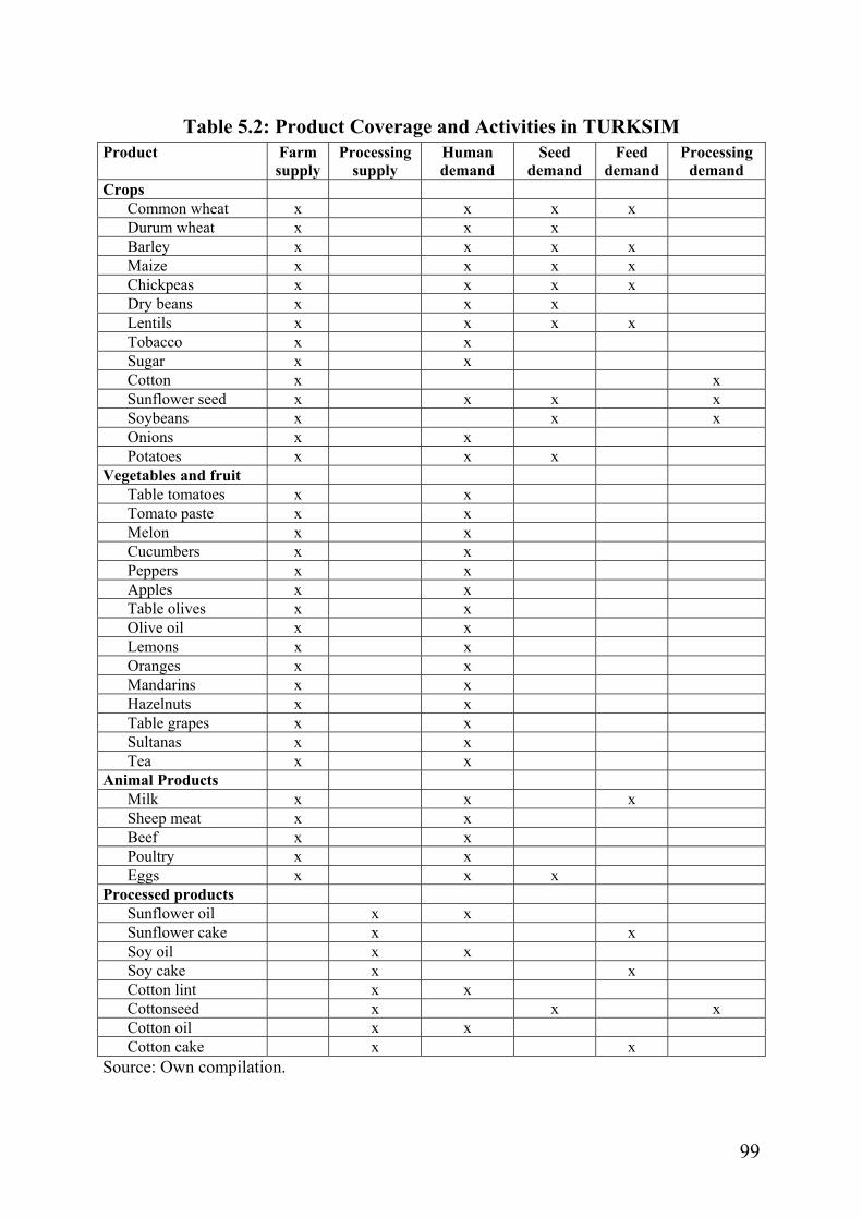
99

Table 5.2: Product Coverage and Activities in TURKSIM Product Farm

supply Processing

supply Human demand

Seed demand

Feed demand

Processing demand

Crops Common wheat x x x x Durum wheat x x x Barley x x x x Maize x x x x Chickpeas x x x x Dry beans x x x Lentils x x x x Tobacco x x Sugar x x Cotton x x Sunflower seed x x x x Soybeans x x x Onions x x Potatoes x x x

Vegetables and fruit Table tomatoes x x Tomato paste x x Melon x x Cucumbers x x Peppers x x Apples x x Table olives x x Olive oil x x Lemons x x Oranges x x Mandarins x x Hazelnuts x x Table grapes x x Sultanas x x Tea x x

Animal Products Milk x x x Sheep meat x x Beef x x Poultry x x Eggs x x x

Processed products Sunflower oil x x Sunflower cake x x Soy oil x x Soy cake x x Cotton lint x x Cottonseed x x x Cotton oil x x Cotton cake x x

Source: Own compilation.

100

For all twelve crops, seventeen vegetables and fruit, and five animal products, supply is defined at farm level. Olive oil and tomato paste, which of course are processed products, are classified as "vegetables and fruit” in TURKSIM as the processing activity is not modeled explicitly, i.e. as for other farm products, the area allocated to the production of tomato paste and olive oil is defined as well as the yield of those products per ha. The processing activity is implicitly covered by the high margin between the farmgate price (e.g. for tomatoes per ton of tomato paste, entering the processing industry) and the wholesale price (for tomato paste).39 Human demand is defined for each of the farm products except cottonseed and soybeans, which directly enter the processing industry for the separation of seed and lint (cotton) and oil and cake/meal (soybeans). Seed demand is defined for those products for which seed accounts for a significant share of production. In the case of eggs, seed demand is to be interpreted as demand for hedging eggs. Processing demand is defined for raw cotton (equation 5.17) as well as for oilseeds (equation 5.18). In the case of sunflower seed, processing demand adds to human demand at the unprocessed level. For the other processing inputs, processing demand is the only demand component except, in some cases, seed demand. Feed demand is defined for various farm products as well as for three processing outputs (oil cake). For oil cake, feed demand is the only demand component. For all other feed products, feed demand adds to human demand.

Table 5.3 shows, that TURKSIM covers a high share of Turkish agricultural production. For the year 1999, TURKSIM covers about 96 percent of Turkish crop production, 78 percent of vegetable production, and 67 percent of fruit production. Altogether 83 percent of plant production and 94 percent of animal production is accounted for.

39 This approach is chosen because, in contrast to the oilseed industry, processing inputs usually are not traded, and the quantity of the raw product produced is therefore identical with the quantity processed. In addition, and in contrast to raw cotton, processing modeled in equation (5.11), these processing activities transform a single product (tomatoes, olives) into a single output (tomato paste, olive oil).

101

Table 5.3: Value Shares of Products Covered by TURKSIM (1999)

Value (mill. €)

Value share

Value (mill. €)

Value share

Crops Fruit Wheat 3,045 28.0% Olives 531 8.1% Barley 1,024 9.4% Lemons 218 3.3% Maize 391 3.6% Oranges 282 4.3% Chickpeas 303 2.8% Mandarins 137 2.1% Dry beans 206 1.9% Grapes 1,429 21.9% Lentils 106 1.9% Apple 834 12.8% Tobacco 848 7.8% Hazelnuts 922 14.1% Sugar beet 1,052 9.7% TURKSIM

fruit 4,353 66.7%

Cotton 898 8.2% Other fruit 2,170 33.3% Sunflower 474 4.4% Total fruit 6,523 100.0% Onions 571 5.2% Potatoes 1,374 12.6% TURKSIM crops 10,392 95.5% Other crops 493 4.5% Total crops 10,885 100.0% Vegetables Animal Tomatoes 1,893 34.6% Milk 3,841 41.2% Watermelons 642 11.8% Beef 1,768 19.0% Melons 415 7.6% Sheep 1,279 13.7% Cucumbers 500 9.2% Poultry 1,035 11.1% Peppers 791 14.5% Eggs 825 8.9% TURKSIM

vegetables 4,241 77.6% TURKSIM

animal 8,748 93.9%

Other vegetables 1,223 22.4% Other animal 569 6.1% Total vegetables 5,464 100.0% Total animal 9,317 100.0% Total value of plant products covered by TURKSIM 18,986 Total value of plant products 22,872 Value share of TURKSIM products 83.0% Total value of agr. products covered by TURKSIM 27,734 Total value of agricultural products 32,189 Value share of TURKSIM products 86.2% Sources: SIS (2000), Agricultural Structure; own calculations. Note: Throughout this study product classification into crops, vegetables, and fruit is done according to the classification used by the SIS.

102

5.3 Integration into the International Trade Environment

5.3.1 Basic Approach

Price formation at the domestic market takes place at the wholesale market level. During model solution, the level of the domestic wholesale price can be determined in three ways:

1. In a net importing situation, the domestic wholesale price is at the import-based level.

2. In a net exporting situation, the domestic wholesale price is at the export-based level.

3. In a no net trade situation, the domestic price is between the export-based and the import-based level. In such a situation the domestic wholesale price is determined by the equilibrium of domestic supply and demand.

Graph 5.1 below depicts these three options modelled in TURKSIM.

Graph 5.1: Domestic Price Formation in Different Net Trade Situations

At the vertical axis various prices and margins are shown. Due to international transportation cost the cif price exceeds the fob price. In the absence of any border policies at the export side the export based price (Peb) is determined by the fob price plus any margin due to domestic transportation and quality, which

Price D2 D3 D1 S Pib t qual Pcif Peb qual Pfob Quantity

103

is assumed to be positive in this example (qual). The import based price (Pib) is determined by the cif price plus a quality/transportation margin (qual) and any border policies at the import side, in this example a tariff (t).

If the demand curve is at D1, demand exceeds national supply S at Pib, and the country is in an importing situation. If the demand curve shifts left to D2, supply exceeds demand at Peb and the country is in an exporting situation. If the demand curve is at D3 a domestic market equilibrium exists with the price being below Pib but above Peb.

The adjustment of the internal price resulting from a changing net trade situation, whether it results from trade policy, world market price changes, or a shift of the supply or demand curve, takes place smoothly. This is shown in Graph 5.2 for a situation in which increasing domestic demand, ceteris paribus, induces price changes.

Graph 5.2: Domestic Price Formation in Different Net Trade Situations

In an exporting situation, in which net exports (NX) are positive, the internal price is at Peb. If net imports reach zero due to the demand curve shifting to the right, the domestic price increases along the price line, determined by the equilibrium of internal supply and demand. This price change does not necessarily assume a linear course as sketched in Graph 5.2, but rather depends on the selected functional forms of domestic demand and supply as well as on exogenous factors like population or productivity growth which determine their

Price Pib Peb Domestic demand NX > 0 NX = 0 NX <0

104

position. If the price line reaches the import based level, net exports become negative and the domestic price remains constant with increasing net imports.40

5.3.2 The Generation of Border Prices and the Link to the Domestic Price Level in the Base Situation

For the base situation, domestic wholesale prices and import or export prices are observed prices.41 If import-export prices are multiplied by the exchange rate and the relevant border policies (export subsidies, tariffs) are added one would expect these "border prices" to be close to the observed domestic prices. But this is not always the case; considerable margins, positive or negative, can be observed in many cases between domestic and border prices. Various factors can contribute to these margins. They are discussed here in the context of an importing situation, but would be similar in an exporting situation, as well:

• Transportation cost: the location of the domestic price observation can be closer or further from the main consumption regions than is the place of importation. The domestic price can therefore be higher or lower than the import price. In addition, a marketing margin of the importing company could result in the domestic price being above the import price.

• Quality differences: the imported product could be of higher or of lower quality than the average domestic product. The domestic price can therefore be higher or lower than the import price.

• Differences in packaging: the imported product can be packaged more or less ready for consumption than the product for which a domestic price is reported. For example, vegetable oil may be imported in tanks, while domestic wholesale oil is in 1 or 5 liter containers. The domestic price can therefore be higher or lower than the import price.

40 In order to solve TURKSIM such that the resulting net export position is in accordance with the wholesale price level chosen (Pib, Peb, or domestic), an iterative procedure is applied. First, all domestic wholesale prices are set at Peb level and the model is solved. In a loop over all products the domestic price is then set at Pib level if results of the first run indicate net exports below zero, and the model is solved again. If the resulting net exports are positive, net exports are fixed to zero and the model is solved again such that domestic demand equals domestic supply. The change of the net trade position of any product can, due to various cross-price relations at the demand as well as at the supply side, cause a change in the net trade position for any other product. Therefore this procedure is repeated several times until the net trade position remains stable.

41 In some cases the farmgate prices are the observed prices and wholesale prices are calculated by adding a processing margin. See Subchapter 7.2.

105

• Indirect import restrictions, e.g. restrictive import licensing can raise the domestic price above the border price.

How are these price margins to be handled in a model? For TURKSIM, product specific assumptions are made about the size of the transportation margin and, in some cases, about indirect border measures like implicit export subsidies financed by budgetary losses of state trading enterprises. The residual is considered a quality margin. Before explaining the procedure in detail, Table 5.4 presents the parameters and sets used for establishing the link between domestic and border prices.

Table 5.4: Parameters and Sets Used for Establishing a Link between Domestic and Border Price

Price parameters Margins

p_ws Domestic wholesale price cfsp Cif-fob spread

p_eb Export-based price tr_im Transportation cost in an importing situation

p_ib Import-based price tr_ex Transportation cost in an exporting situation

p_ex Export price qual Quality margin

p_im Import price Policy parameters

p_wm World market price t_av Ad valorem tariff

chg_wm World market price change t_sp Specific tariff

pr_tr Price transmission es Export subsidy

er Exchange rate

Sets

Abbrev. Description External parameter Calculated parameter

ib Products for which the domestic price in the base situation is linked to the import price

p_ws, p_im, cfsp, tr_im, tr_ex, er

p_ex, qual, p_eb

eb Products for which the domestic price in the base situation is linked to the export price

p_ws, p_ex, cfsp, tr_im, tr_ex, er

p_im, qual, p_ib

dom_ib Products for which the domestic price is not linked to a border price in the base situation, import price observed

p_ws, p_im, cfsp, tr_im, tr_ex, er, qual

p_ex, p_ib, p_eb

dom_eb Products for which the domestic price is not linked to a border price in the base situation, export price observed

p_ws, p_ex, cfsp, tr_im, tr_ex, er, qual

p_im, p_ib, p_eb

sc Scenarios (base and simulations) Source: Own compilation.

106

The top of Table 5.4 presents price, margin and policy parameters which are used in establishing the link between domestic and border prices. The lower part shows the four categories into which tradable products are classified, and indicates which parameters are external parameters and which are calculated internally for each of these categories. For each of the categories, the establishment of border prices is described in detail below.

The category ib includes products for which significant net imports are observed in the base period, and therefore the domestic wholesale price (p_ws) is assumed to be linked to the import price (p_im). In such a situation, p_ib is set equal to p_ws. The quality margin, the export price, and the border price, which would occur in an exporting situation (p_eb) under the base situation, are then calculated as follows.

The quality margin is determined as the residual of the wholesale price minus the import price multiplied by the exchange rate (er) plus tariffs (ad valorem and specific) and a transport margin in an importing situation (tr_im):

(5.24) qual = p_ws – p_im • er • (1+t_av) + t_sp + tr_im.

The export price equals the import price minus the cif-fob spread (cfsp):

(5.25) p_ex = p_im – cfsp. The border price which would occur in an exporting situation (p_eb) equals the export price multiplied by the exchange rate plus any export subsidy (es), a transport margin (tr_ex), and the quality margin as determined in (5.24):

(5.26) p_eb = p_ex • er +es + tr_ex +qual.

The set eb includes products for which significant net exports are observed in the base period, and therefore the domestic price is assumed to be linked to the export price. In such a situation p_eb is set equal to p_ws. The quality margin, the import price (p_im), and the border price, which would occur in an importing situation (p_ib), are then calculated as follows:

(5.27) qual = p_ws – (p_ex • er + es + tr_ex),

(5.28) p_im = p_ex + cfsp, and

(5.29) p_ib = p_im • er • (1+t_av) + t_sp + tr_im + qual.

For some products, no significant trade exists in the base situation and the domestic wholesale price is therefore assumed to be determined by domestic supply and demand. These products are included in sets dom_ib and dom_eb. Border prices must be established for these products as well to allow for a shift

107

towards a net exporting or a net importing situation in the course of the simulation process. To this end an export price (in case of dom_eb) or an import price (in case of dom_ib) for the product concerned is chosen such that it is as "representative" as possible for the domestic quality. This allows for the omission of the specification of any quality margins in those cases. In the case of dom_ib, border prices are established as follows:

(5.30) p_ib = p_im • er • (1+t_av) + t_sp + tr_im,

p_ex is obtained according to (5.25), and

(5.31) p_eb = p_ex • er +es + tr_ex.

For dom_eb, prices are determined in analogy, the only difference is that the export price is external and the import price is determined according to (5.28).

5.3.3 The Generation of Border Prices and the Link to the Domestic Price Level in Simulations

Changes in border prices between the base situation and the simulations can be caused by two factors: changes in world market prices, and changes in border policies. These changes are introduced in TURKSIM as follows. World market price changes for each scenario and product are specified externally and applied to the respective import and export prices in the base period. The relative changes of world market prices under the simulations are also applied to the quality margins. The underlying assumption is that different qualities are very close substitutes and relative prices therefore remain constant.

All border policy parameters (es, t_av, t_sp) are defined for each scenario, and border prices are calculated according to (5.26) and (5.29), based on the respective import/export prices, policy parameters, and quality margins.

Based on these mechanisms the extent of price transmission from changing border prices to domestic prices differs according to the net trade poition:

1. The relative change of the border price is almost fully transmitted to the domestic price if the net trade position does not change (only specific tariffs, export subsidies and transport margins do not vary with the border price). In this case, the price transmission elasticity is close to one.

2. The change of the border price is only partially transmitted to the domestic price if the net trade status changes.

108

3. The change of the border price is not transmitted to the domestic price if price formation is domestic in the base situation and in the respective simulation.

For some products for which transportation costs are high, the mechanism described above seems questionable. This is especially the case for meat and dairy products. Most of these products require chilled transportation and storage from the point of entry to the retail level. These requirements are costly and, in some local markets may be unavailable. As a result, even in a clear net importing situation, price transmission from border price to domestic price may, on national average, be significantly below unity as some local markets are separated from the border price. In order to model this effect, a price transmission parameter (pr_tr) is introduced, which is usually fixed at unity but, in some cases, may be set below one and influences the change in border price:

(5.32) p_ebsc, i = p_ebsc = base, i + pr_tri • (p_ebsc, i - p_ebbase,i),

with the import based price determined accordingly.42

5.4 Farm Supply Model

Domestic price formation takes place at the wholesale price level as described above. But agricultural producers base their production decisions on farmgate prices. Farmgate prices are linked to wholesale prices according to:

(5.33) P_WSfarm = P_FGfarm/(1-waste_perc) • (1+pm_r) + pm_a.

The processing/trade margin between farmgate and wholesale price consists of three elements. First, the wholesale price is higher than the farmgate price due to physical postfarm losses during transportation or processing which must be compensated by higher selling prices. Secondly, a relative margin is added (pm_r), which consists of processing/trade costs relative to the product value, e. g. circulating capital cost or insurance cost for product transactions. Thirdly, an absolute margin (pm_a) is specified per product unit, which includes physical transportation or processing costs.

In addition to the farmgate price as specified above, a government premium directly linked to the unit produced can separate the effective farmgate price on

42 In order to guarantee consistency of the price and policy data fed into the model, import based and export based prices are compared for all scenarios and if p_eb > p_ib for any product, the program is aborted and displays the import- and export-based border prices calculated so that necessary adjustments can be made.

109

which producers base their decisions (P_EFfarm) from the observed farm gate price according to equation (5.19). 5.4.1 Plant Products

5.4.1.1 Basic Mechanisms Farm supply of plant products is defined on a regional level and is separated into allocation of area and yield. Allocation of area is modeled according to:

(5.34) el_arpl,pls,reg

pl,reg pl,regpl,reg pls regpls

= • + • int_ar P_EF ad_ha SHAREAREA ∏ .

Explanatory variables for area allocation are effective own and cross farmgate prices which are determined according to (5.19). The parameter ad_hareg is zero in eight out of nine regions, as the effect of additional irrigation area is only modeled for the Southeast Anatolia irrigation project (see Section 5.3.1.2). Regional own- and cross-price elasticities (elpl,pls,reg), as well as intercepts (int_arpl,reg), are external parameters, the latter calculated within the program code from base data and elasticities. Elasticities, chosen based on literature and plausibility considerations (see Section 6.2.1), are composed such that the conditions resulting from economic theory, namely non-negativity of the own price effect, symmetry of cross price effects and homogeneity of the supply function are met. Symmetry, however, can only be met locally due to the functional form chosen. For a detailed description of the implementation of the conditions following from economic theory (see Subchapter 6.2).

TURKSIM allows for the modeling of products which are restricted by supply quotas. In its current version, sugar is the only product concerned and supply is modeled as follows. Sugar supply in the base situation is restricted and an assumption on the level of the shadow price in the base situation enters the model as an exogenous parameter (e.g. p_shpl, sc = base = p_fg pl, sc = base • 0.8).43 All area allocation functions are calibrated with respect to the shadow price of the product restricted instead of the effective farmgate price. Scenarios are divided into those with (sc_q) and without (sc_nq) a restrictive quota. For the former, the national quantity quota enters the model as exogenous parameter and is allocated to regions according to the production share in the base situation, and regional area restrictions are defined according to equation (5.2) above. In quota scenarios, area allocation for quota products is determined as equalling the regional area quota and a shadow price is calculated for each region by substituting the area restriction (QU_R) for AREA according to equation (5.35):

43 The assumption of the shadow price for sugar being at 80 percent of the farmgate price is crucial for modeling changes in the quota regime, but the empirical foundation is weak.

110

1el_ar pl_q,pl_q,reg

pl_q,reg

pl_q,regel_ar pl_nq,pl_nqs,reg

pl_q,reg pl_nqspl_nqs

QU_R = P_SH

int_ar P_EF •

∏

(5.35)

The calculation of shadow prices in quota scenarios is necessary to allow for correct area allocation for cross products, and for the precise calculation of welfare effects from changes in the quota system (see Section 5.7.1). In nonquota scenarios, area allocation for all products is assumed to take place according to (5.34).

Explanatory variables for area allocation do not include input prices. This is because reliable data is difficult to collect and variable inputs make up a relatively low share of the product price. In addition, no policy simulations are intended for variable inputs. Production factors capital, land, and labor, in the main family labor, are assumed to be relatively fixed in Turkey and therefore are not considered. Nonetheless, the cost share of variable inputs is implicitly considered by implementing the homogeneity condition for supply functions (see Subchapter 6.2).

Regional yield is modeled as

(5.36) el_yipl,regpl,reg pl,reg pl pl = • • int_yi P_EF prodYIELD .

The only explanatory variable is the own effective farmgate price. Exogenous parameters are a product specific productivity shifter (prodpl), the elasticity of yield with respect to the own price (el_yipl,reg) and the intercept (int_yipl,reg), which is calibrated based on the base period data. Other possible explanatory variables would be the prices of variable inputs (fertilizer, pesticides). However, the same argument as for area allocation applies: average cost shares of variable inputs in Turkish agricultural production are so low that resulting elasticities and impact on yield are very low (GRETHE, 1999, p. 37). Therefore input prices are not included as explanatory variables in TURKSIM. Regional supply of plant products is defined according to equation (5.4) as the product of regional yield and regional area.

5.4.1.2 Additional Irrigation Area The additional irrigated agricultural area which will be available under the Southeastern Anatolia Project (Güneydogu Anadolu Projesi, GAP) in the years to come is expected to have a major impact and must therefore be considered

111

when projecting future agricultural production. The GAP is a large scale regional development project covering six provinces with about 10 percent of national land area. The core element of the GAP is the use of the Euphrates and Tigris rivers for irrigation and hydropower generation. At the final stage of the project almost 1.7 million ha of agricultural land will be irrigated compared to about 200,000 ha in the model base period (1997/99). This includes about 1.5 million ha to be converted from dry agricultural land to irrigated land, an additional 40 percent compared to the national irrigated area in the base period. There have been different views on the timetable of implementation of the GAP irrigation scheme and the implementation schedule has been postponed repeatedly. The Southeastern Anatolia Project Master Plan Study (STATE PLANNING ORGANIZATION, 1990, Vol. I, p. 10) scheduled priority irrigation schemes of 894,000 ha to be completed by the year 2005. Another study presumed 1,400,000 ha under irrigation by the year 2005, expecting the irrigation scheme to be fully realized in 2010.44 Experts in the GAP Regional Development Administration and in the Ministry of Agriculture and Rural Affairs (MARA) currently expect some additional 300,000 ha to be irrigated in 2006 compared to the 1997/99 base situation of TURKSIM. This will change Turkey's agricultural production in 2006 if compared to the base situation for various reasons: i) land will be shifted from traditionally grown crops to crops with higher water requirements, ii) yield will increase, and iii) secondary crops will be grown on part of the land.

It is difficult to accurately assess the impact of additional irrigated area in TURKSIM because the difference between production on irrigated and on nonirrigated area is not explicitly modeled. A simple approach to shift supply curves right for selected products is chosen which allows for the inclusion of a priori knowledge, e.g. specific studies on future production programes in the GAP region, and at the same time, lets relative prices under different scenarios have an impact on allocation of newly irrigated area.

To this end the set of regions is divided into two subsets, those covered by the GAP project (reg_irr) (Southeast Anatolia) and those not covered by the GAP project (reg_n_irr). As only one region is covered by the GAP project, the variables SHARE, AR_PRE, and AR_PRE_T below are not indexed with respect to regions, as they apply only to one region in the current version. In case of Southeast Anatolia, ad_ha (see equation 5.34) is an external parameter

44 Southeastern Anatolia Project Regional Development Administration, (1992) Agricultural Commodities Marketing Survey, Planning of Crop Pattern and Integration of Marketing and Crop Pattern Studies; for simplicity, hereafter referred to as Marketing Survey and Crop Pattern Study.

112

indicating the irrigation area available for additional production, which is set at zero in the base run and takes a positive value in all simulations.45 The SHARE variable indicates which share of ad_ha is allocated to each product. Plant products are divided into three subsets in order to determine SHARE:

1. non_irr Products which do not take a share of ad_ha

2. irr1 Products for which strong a priori assumptions on area coverage exist from external sources

3. irr2 Other products For subset non_irr SHARE equals zero. For subset irr1 SHARE is determined as follows:

(5.37) SHAREirr1 = irr_wirr1 • AR_PREirr1 / AR_PRE_T,

with AR_PREirr1 being the area allocated to product irr1, which would occur in the respective scenario with ad_ha equaling zero and AR_PRE_T defined as:

(5.38) AR_PRE_T = ∑irr1 AR_PREirr1.

The term irr_w is an external parameter defined for each product ∈ {irr1}, which is multiplied by the share, the respective product covers under the respective scenario, without additional area (AR_PREirr1 / AR_PRE_T).

For subset irr2, SHARE is determined by dividing the remaining irrigated area available among irr2 products according to the shares they would cover under the respective scenario with ad_ha equaling zero:

(5.39) SHAREirr2 = (1 - ∑irr1 SHAREirr1) • AR_PREirr2 / ∑irr2 AR_PREirr2.

Should any products restricted by a binding supply quota be elements of sets irr1 or irr2, SHARE for the respective product is set at zero and the calculation of SHARE for other products is adjusted accordingly. For details, see the GAMS code; for the determination of ad_ha and irr_w, see Subchapter 8.4.

5.4.2 Animal Products

Animal supply is modeled on a regional level according to equation (5.40):

(5.40) el_sa el_sfan,ans,reg an

anan,reg an,reg ans anans

= • • • F_SUP int_sa P_EF prodFCI∏ .

45 ad_ha is not identical with the total additional irrigated area, as part of this area is assumed to be used to maintain current production. See subchapter 8.4 below.

113

Explanatory variables are own and cross effective farm gate prices (P_EF) as well as a feed cost index (FCI). The regional elasticities of animal product supply with respect to animal product prices (el_saan,ans,reg) and the feed price (el_sfan), as well as the productivity shifter (prod), enter the model as exogenous parameters. The intercept of the supply function (int_saan, literature reg) is calibrated according to base period data. Elasticities, chosen based on and plausibility considerations (see Section 6.2.2), are composed such that non-negativity of the own price effect and homogeneity of the supply function in all prices hold globally, and symmetry of cross price effects holds locally.

114

5.5 Feed Model

An overview of the feed model in TURKSIM is shown in Figure 5.1.

Figure 5.1: Schematic Overview of the Feed Model

Demand for feed components per unit of animal product (1) is dependent on wholesale prices of feed components.46 This relationship is shown in equation (5.41):

(5.41) el_fdfe,fes

fe,an fe,an fesfes

= • F_DEM int_fd P_WS∏ .

Own and cross price elasticities of feed demand (el_fdfe,fes) as well as intercepts (int_fdan) are external parameters, the latter calibrated from base data. Elasticities are chosen based on literature and plausibility considerations (see Section 6.3.3), and are composed such that nonpositivity of the own price effect and homogeneity of the feed demand function in all feed prices (including fodder and pasture for ruminants) hold globally and symmetry of cross price

46 This probably represents the situation well for poultry and egg production, which is organized industrially and mainly relies on purchased compound feed. For red meat and milk production, however, it may be more appropriate to use farmgate prices of feed components as explanatory variables, as a large share of animal feed is produced on the farm.

(4 ) R e g io n a l fe e d d e m an d = (1 ) • (3 )

(3 ) A n im a l s u p p ly

(2 ) F C I ( fe e d p r ic e p e r to n )

(1 ) F e e d c o m p o n e n t d e m an d /an im a l

p ro d u c t u n it

C o m p o n e n t p ric e s

A n im a l p ro d u c t p r ic e s

115

effects holds locally. From the resulting feed composition and component prices a feed cost index (FCI) is calculated according to (5.42):

(5.42) FCIan = ∑fe (P_WSfe • F_DEMfe,an/∑fe F_DEMfe,an).

The feed cost index and effective farmgate prices for animal products determine animal supply (3) as defined in equation (5.40) above. Regional feed demand (4) is the product of (1) and (3), as defined in equation (5.9).

Due to this modeling approach, an increasing feed price for any feed component results in reduced demand for this component due to two effects. First, the substitution effect, which results in other components substituting for the more expensive one according to (5.41), and second, the output effect which results, via an increasing FCI, in lower animal production and therefore lower feed demand.

5.6 Processing Model

Two different kinds of processing activities are defined. Processing demand for inputs which are nontradable (set pr_in1; only raw cotton in the current version) is defined according to equation (5.11) above. Processing demand for tradable inputs (set pr_in2; three oilseeds in the current version) is defined as:

(5.43) el_po el_pipr_in2, pr_out2 pr_in2

pr_in2 pr_in2 pr_out2 pr_in2pr_out2

= • • P_DEM int_pd P_WS P_WS∏ .

Explanatory variables are wholesale prices for processing inputs and outputs. The intercept (int_pd), as well as the elasticities of processing demand with respect to output prices (el_po) and input prices (el_pi), are exogenous parameters, the former calibrated according to base data. Equation (5.43) is restricted to be homogenous of degree zero in all input prices (price elasticities with respect to inputs other than oilseeds are taken into account, see Section 6.3.4).

Processing supply is defined as processing demand multiplied by the respective extraction factor:

(5.44) PR_SUPpr_out = PR_DEMpr_in • exfpr_out.

5.7 Demand Model

Human demand is modeled for income quintiles according to equation (5.45).

(5.45) el_hd el_inci,j,inc i,inc

i,inc i,inc jj

= • • • popH_DEM int_hd P_WS income∏ .

116

Explanatory variables are own and cross prices. Income group-specific elasticities of demand with respect to own and cross prices (el_hdi,j,inc), and to income (el_inci,inc), as well as income and population shifters (income, pop) and the intercept, are exogenous parameters, the latter calibrated according to the base data set. Elasticities are based on own estimates, literature, and plausibility considerations (see Sections 6.3.1 and 6.3.2) and are composed such that nonpositivity of the own price effect and homogeneity of degree zero of demand functions in compensated price elasticities hold globally and symmetry of cross price effects, as well as the adding up condition, hold locally.

Processing demand and feed demand are explained in Subchapters 5.4 and 5.5 above. Seed demand is defined according to equations (5.13) and (5.14) and total demand according to equation (5.15) above.

5.8 Welfare Calculations

Welfare effects under each simulation scenario are evaluated as welfare changes compared to a reference simulation. In the current TURKSIM version, the status quo scenario simulating a situation with unchanged agricultural policies at the end of the projection period, is chosen as the reference scenario. Welfare effects are calculated at farm level, at the level of human consumption, and at the level of the processing industry, and, together with budgetary effects, are summed as total welfare effects.

5.8.1 Welfare Changes at Farm Level

If only a single price change of one input or output is considered, the change in producer surplus measured as the definite integral of the supply function from p0 to p1 is the correct measurement for the change in producer welfare (JUST et al. 1982, pp. 55 ff.). For the evaluation of welfare changes in TURKSIM, however, multiple simultaneous price changes must be taken into account. Consider, for example, the case of two substitutes whose prices change simultaneously as presented in Graph 5.3:

117

Graph 5.3: Welfare Changes with Simultaneous Price Changes

If the price for wheat (left hand panel) rises from Pw0 to Pw1 and wheat supply rises, the supply curve for barley (Sb), a close substitute, shifts left as more area is allocated to wheat and the barley price increases due to lower barley supply. The increasing barley price, in turn, results in the wheat supply curve shifting left. For a correct determination of the resulting welfare change, price changes must be evaluated stepwise. First, the change in producer surplus for one product must be evaluated under the original supply curve (e.g. the grey shaded area in the left hand panel), and second, the price change for the next product is evaluated under the new supply curve for the product concerned (e.g. the grey shaded area in the right hand panel). This sequential approach can be extended to input prices and the results are not dependent on the path of integration if cross effects are symmetrical.47 As a result, welfare changes at the producer side are determined:

(5.46)

where Pi is the price of product i, SUPi is the supply function of product i, Wj is the price for input j, and FDj is the factor demand function for input j.

47 For an algebraic deduction see JUST et al. (1982, pp. 338 ff).

Pw1

Pw0

Wheat quantity

Sw1

Sw0

Pb1

Pb0

Barley quantity

Sb1

Sb0

ji

i j

11n m

i ji=1 j=10 0

W P• dW • dP - ,FDSUP ji

P W∑ ∑∫ ∫

118

In TURKSIM, supply functions for plant products include product prices as independent variables only. Therefore equation (5.46), with abbreviations as used in TURKSIM, reduces to:

(5.47) .

In TURKSIM, changes in producer surplus are calculated according to (5.47) with prices changed sequentially. The respective definite integrals are multiplied by 1-(seedpl_nq/yieldpl_nq). This is because seed production is assumed to stay at the farm. Therefore welfare changes should not be calculated for this part of production, as the farmer is also the consumer.

Initially, price changes are introduced and definite integrals are calculated for all nonquota products. As a final step, welfare changes for quota products are calculated (only sugar in the current TURKSIM version). Starting from a situation in which the quota is binding (scenario s_quo), i.e. the shadow price is below the effective farmgate price for sugar, there are different possibilities for the resulting welfare effects. Should the quota system be abolished, the calculation of the welfare effects depends on whether the new price is below or above the shadow price of the reference scenario (see Graph 5.4).

Graph 5.4: Welfare Changes Resulting from an Abolition of a Quota System

The left hand panel of Graph 5.4 shows a situation where the new price is above the shadow price of the reference situation. The resulting welfare effects are composed of a loss in quota rent (area "-") and a gain in producer surplus due to

P0

P1

Supply

S

P_SH0

-+

Price

a

P0

P1

Supply

S

P_SH0

-

Price

--

1,

pl n

pl plpl=10

, pl

P_EF•F_SUP dP_EF

P_EF∑∫

119

the expansion of production (area "+"). Area "+" is determined in TURKSIM by taking the definite integral of S between P1 and P_SH0 and subtracting area "a".

The right hand panel of Graph 5.4 shows a situation in which the new price is below the shadow price of the reference situation. In such a case the welfare effect is composed of the loss in quota rent resulting from the market price decreasing until it reaches the level of the shadow price (upper rectangle "-"), and the loss in producer surplus resulting from a further decreasing market price (lower area "-"), that is, the definite integral of S between P_SH0 and P1.

In the case of a binding quota in the new situation, possible effects are also manifold. Graph 5.5, as an example, shows a situation where a welfare loss due to a decreased market price (area "-") is combined with a welfare gain due to an expanded quota quantity (area "+").48

Graph 5.5: Welfare Changes Resulting from a Change in the Quota System

Welfare changes which result from production on newly irrigated areas (see Section 5.3.1.1) are linearly approximated by multiplying the price change by the average supply quantity on the newly irrigated area:

(5.48) (P_EFpl, sc_wf - P_EFpl, s_quo) • (ad_ha •SHAREpl, s_quo • YIELDpl, s_quo / 1000 + ad_ha •SHAREpl, sc_wf • YIELDpl, sc_wf / 1000)/2.

48 The automatic calculation of welfare effects in a scenario with a binding quota for all possible combinations of price and quota changes is not yet programmed in TURKSIM. The CU scenario is the only scenario for which the change in producer surplus is calculated with the quota system maintained, and the respective calculation is included in the code.

P0

P1

Supply

S

P_SH0

-

Price

+

Q0 Q1

120

Welfare changes for animal producers are also calculated by introducing changes in product prices sequentially and summing up the definite integrals below the supply curves. Welfare changes of changing feed prices are taken into account by linear approximation (multiplying the change in FCI by the average feed quantity). This is for computational simplicity as feed demand functions for individual components, following from equations (5.40), (5.41), and (5.42) are rather complex:

(5.49)

The sequential introduction of price changes for the evaluation of welfare effects means that results for individual products cannot be interpreted and compared properly. This is because the size of the welfare change for individual products depends on how many cross prices have already been changed, and thus on the path of integration. Therefore welfare changes in TURKSIM are also calculated as definite integrals under supply and demand curves with only the own price changing. These results cannot be used to evaluate the total welfare change, as cross prices are not considered, but it allows for the comparison of welfare changes for individual products due to own price changes.

If supply and demand functions are derivatives of a profit/indirect utility function, the resulting cross effects are automatically symmetric, as they are second derivatives of the same function. This is not the case for the systems of supply and demand functions applied in TURKSIM, as they are not derivatives of any profit/indirect utility function. For this reason, symmetry can be introduced only locally. Symmetry, however, is required for the path independence of the sequential approach of analysis of the welfare effect in case of multiple price changes applied in TURKSIM (JUST et al., 1982, p. 340). A sensitivity analysis with respect to the path of integration was therefore applied. Maximal changes in total consumer welfare or producer surplus due to a change in the path of integration were found to be 0.4 percent. This is significantly below the deviation of the results of the nonsequential approach from the sequential approach, which was up to 3 percent of the compensating variation and the change in producer surplus. As a result, the nonsequential approach was found to overestimate the welfare gains from liberalization by about 18 percent whereas the welfare gain under the liberalization scenario according to the

( )el_sael_fd an,ans,regfe,fes

fe,an fes an,reg ans anfes ans

el_sf ananel_fd el_fdfe,fes fe,fes

fe fe,an fes fe,an fesfefefes fes

• • • • int_fd P_WS int_sa P_EF prod

• P_WS int_fd P_WS int_fd P_WS• • / •

∏ ∏

∑ ∑∏ ∏∑

121

sequential approach differed no more than 2.7 percent with respect to the path of integration. Therefore, the results of the sequential approach are used as the indicator of choice for total welfare effects throughout this study even if they are not completely unequivocal.

5.8.2 Welfare Changes at the Consumer Level

At the demand side, welfare changes should not be evaluated as definite integrals below the ordinary demand curves, as this measure would, for superior goods, underestimate welfare losses and overestimate welfare gains as the income effects are not adequately treated. A correct measure, instead, is the calculation of the compensating variation which is the definite integral below the compensated demand curve (LAYARD and WALTERS, 1978, p. 146). In case of multiple simultaneous price changes, welfare changes should be evaluated with the stepwise introduction of price changes as has been described for the supply side above (LAYARD and WALTERS, 1978, p. 147). Therefore welfare changes at the human demand level are calculated in TURKSIM according to

(5.50)

1,

i n

i ii=10

, i

P_WS•H_DEM_C dP_WS

P_WS∑∫ ,

with prices changes being introduced sequentially and H_DEM_Ci being the compensated demand curves. The respective compensated demand curves are calibrated based on compensated demand elasticities (see Chapter 6), and based on prices after introduction of each sequential price change.

5.8.3 Welfare Changes at the Level of the Processing Industry

Welfare changes for the processing sector are evaluated only for that part of the processing industry for which processing demand varies according to the processing margin (equation 5.43; oilseed crushing industry) and thus not for cotton gins. Price changes for inputs and outputs are introduced sequentially and definite integrals are taken of the respective processing demand (5.43) and processing supply functions (5.44) which are derived from processing demand functions (5.43). The resulting welfare changes are calculated as the sum of definite integrals according to (5.46) for each processing industry.

5.8.4 Budgetary Effects

Budgetary outlays are calculated for each scenario as tariff revenue minus budgetary outlays for export subsidies and producer premiums. Welfare effects are calculated for each scenario as the difference between the budget of the respective scenario and the reference scenario.

123

6 BEHAVIORAL PARAMETERS

6.1 Basic Approach

As all behavioral functions are of the isoelastic type, only supply and demand elasticities enter the model code as exogenous parameters, intercepts are calibrated from base data. The systems of supply and demand elasticities used in TURKSIM are synthetic in the sense that they are not estimated as systems, but individual elasticities stem from various sources such as literature, own estimates, and expert interviews. Nonetheless they are composed such that they have system character as they fulfil most of the requirements of economic theory that apply to interdependent equations, e.g. symmetry of cross price effects and the adding up condition.

Several reasons contributed to the decision not to estimate the full sector model. First, the workload required exceeded the time available for this study as the main focus was on building a simulation model. Second, many estimates, single equations, and supply or demand systems are documented in the literature. This study can partially draw on existing work. Third, the estimation of complete supply or demand systems requires high quality data. In the area of supply analysis, however, data quality in Turkey is limited due to extremely high inflation (around 100 per cent in many years), very limited availability of some data (e.g. input prices and quantities), and political instability influencing production decisions.49 This is especially problematic in the case of simultaneous estimation of supply systems, as any shortcomings of the data do "distribute" through the whole model because of interdependency of supply equations. Even when the available data is of relatively high quality, this can lead to implausible parameter estimates in many cases. For an example of such a case see GRINGS (1985, pp. 188-95).

Many of the data shortcomings at the supply side apply on the demand side, too. This is the case especially for the inflation problem and the political environment. In addition, no time-series data on consumption is available for Turkey. The solution is to generate a time series of demand quantities by adding production and imports minus exports. This data is readily available from the SIS. Changes in stock levels as well as postharvest losses, however, are thus not accounted for and cause distortions. A possible way to include these positions would be to use estimates from FAO commodity balances, which explicitly cover stock changes and losses. Another potential source for distortion of

49 The political instability in south-east Anatolia has contributed heavily to declining ruminant flocks (USDA GAIN Report TU 1034, 21.08.2001, p. 2).

124

consumption data generated in such a way is border trade not covered by official statistics. Especially for trade with former Soviet Union countries, observers estimate this effect to be significant for some products.

Two budget surveys for 1987 and 1994 (SIS, 1990, 1997) are the only available data sets on consumption, which can be used to estimate a set of income elasticities. Because the sample method, classification of income groups and product aggregation are vastly different in these two surveys, they cannot be integrated into one time series. Therefore, no complete demand system including price elasticities can be estimated due to missing time series data. An alternative approach would be the estimation of a linear expenditure system (LES) based on cross section data, for which only one parameter would need to be chosen in order to determine the missing parameters from the income elasticities for the ratio between consumers’ excess income and the income necessary for a minimum consumption basket (TAYLOR, 1979, pp. 220-1). This approach, however, seems questionable when one considers that the level of this parameter is arbitrary and differs heavily among different income groups (PHLIPS, 1983, p. 131). Furthermore, inferior products cannot, due to functional form, be estimated in the LES. Against the background of the high consumption of wheat, especially among the poorer population, a negative income elasticity for wheat seems plausible for lower income groups. In addition, the incapability to represent complementary relations between goods and the linear relationship between income and consumption are disadvantages of the LES (SADOULET and DE JANVRY, 1995, p. 42).

In order to provide some empirical backbone for the framework of demand elasticities, with a view to the crucial importance of the size of income elasticities for projection results over a period with high income growth, a set of demand elasticities with respect to income is estimated based on the 1994 cross section data (see Section 6.3.1). Price elasticities of demand used in TURKSIM are based on literature, plausibility considerations, and the implementation of theoretical requirements (see Section 6.3.2).

For some products, limited transmission of border prices to domestic wholesale prices is included in TURKSIM (see Section 5.2.2 above). The estimation of the respective price transmission elasticities is documented in Subchapter 6.4.

6.2 Supply Side

6.2.1 Plant Products

A matrix is built containing price elasticities of area allocation for all plant products covered by TURKSIM with respect to all prices for plant products covered by TURKSIM, the price of the aggregate of all other plant products, and

125

to the price of variable inputs. This matrix fulfils the symmetry condition and the condition of supply for each product being homogeneous of degree zero in all prices. The price elasticities with respect to the price of other products and with respect to the input price are not used in TURKSIM as they are not variables in the respective area allocation equations (see Subchapter 5.2). Their inclusion in the process of building elasticity matrices, however, is necessary in order to check for fulfilment of the homogeneity condition which applies to all output and input prices.

Own and cross price elasticities of area allocation and yield in TURKSIM are derived according to the following steps:

1. Own price elasticities of area allocation (el_arpl,pl,reg) and of yield (el_yipl,reg) are determined based on literature, expert interviews, and plausibility considerations.

2. Supply elasticities with respect to the price level of variable inputs (el_inpl,reg) are determined for each product based on the cost shares of variable inputs.

3. Plant products are divided into groups of more or less close substitutes.

4. Allen elasticities of substitution (σpl,pls), which are measures for the degree of technical substitutability of products, are determined for each pair of products based on the classification above (3) for one region such that the homogeneity condition of supply is fulfilled for all products:

(6.1) ((el_arpl,pl,reg +1) • (el_yipl,reg +1) – 1) + ∑pls≠pl el_arpl,pls,reg + el_inpl,reg = 0,

with

(6.2) el_arpl,pls,reg = σpl, pls • vpls,reg,

and vpls,reg being the value share of plant product pls in the respective region.

This step is done simultaneously for all products as the homogeneity condition restricts the overall size of Allen elasticities of substitution per product.

5. The resulting Allen elasticities are then transformed into cross price elasticities for the other eight production regions by multiplication with the respective value shares.

6. In case of the homogeneity condition (6.1) being negatively affected, all Allen elasticities for the respective region and product are scaled up or down uniformly in relative terms.

126

Based on this approach, cross elasticities differ among regions only due to the different value shares of the respective products. Further information on differing possibilities of technical substitution among production regions could be introduced in elasticity matrices, but is not included in the current TURKSIM version.

6.2.1.1 Determination of Own Price Elasticities and Cost Shares of Variable Inputs

Table 6.1 presents the own price elasticities, the cost shares of variable inputs, and the resulting supply elasticities with respect to the price of variable inputs. Own price elasticities used in TURKSIM are between 0.22 for tea and 1.73 for several vegetables. Underlying sources and assumptions for the determination of own price elasticities are listed per product below.

Cereals: Elasticities for wheat are long run elasticities taken from the FAO World Food Model (WFM) and are roughly in line with estimates from KASNAKOGLU and GURKAN (1986), BAYANER and HALLAM (1996), and KOC et al. (1998) as well as with elasticities from the SWOPSIM database (USDA, 2002). For barley, the own price elasticity of yield is taken from the FAO WFM. The fact that it is somewhat above the elasticity of yield for wheat is in conformance with estimates from BAYANER and HALLAM. The long run price elasticity of area allocation reported by FAO, however, is 0.71 which is significantly above that for wheat. This ratio of the elasticity of barley area being significantly above that of wheat is not confirmed by estimates of KASNAKOGLU and GURKAN, BAYANER (1996), and KOC et al. Therefore the elasticity of barley area is assumed to be at 0.45, only about 15 percent above that of the area in common wheat. The same approach is applied for corn, where FAO reports an area elasticity of 0.52.

Pulses: BAYANER and HALLAM estimate price elasticities of yield to between 0.56 (lentils) and 0.21 (dry beans), about two to five times those of wheat and barley. BAYANER finds high price elasticities of supply for chickpeas and lentils (around 4.5) but a much lower elasticity for dry beans (0.43). Experts in Turkey believe the price elasticity of area allocation to be relatively low, as rotational considerations are a major factor in determining the area of pulses. For this study the price elasticities of yield are set at 0.24 (twice the yield elasticity of wheat), and the price elasticities of area are set at 0.45, the same level as cereals.

Tobacco: BAYANER and HALLAM find the elasticity of yield being at the same level as for barley. This ratio is also applied for this study. The area elasticity applied in this study is calculated based on an output elasticity being 30 percent below the 1.34 estimated by KASNAKOGLU and GURKAN. This is because alternative estimates (BAYANER) are considerably lower.

127

Table 6.1: Own Price Elasticities, Cost Shares of Variable Inputs, and the Resulting Supply Elasticities with Respect to the Variable

Input Prices Product el_arpl,pl el_yipl el_supplypl,

pl

vpl el_inpl

Crops Common wheat 0.39 0.12 0.56 0.35 -0.19 Durum wheat 0.45 0.12 0.62 0.35 -0.22 Barley 0.45 0.14 0.65 0.35 -0.23 Maize 0.45 0.12 0.62 0.35 -0.22 Chickpeas 0.50 0.24 0.86 0.35 -0.30 Dry beans 0.50 0.24 0.86 0.35 -0.30 Lentils 0.50 0.24 0.86 0.35 -0.30 Tobacco 0.70 0.14 0.94 0.60 -0.56 Sugar 0.70 0.14 0.94 0.60 -0.56 Cotton 0.47 0.19 0.75 0.60 -0.45 Sunflower seed 0.62 0.16 0.88 0.35 -0.31 Soybeans 0.50 0.17 0.76 0.35 -0.26

Vegetables and fruits Onions 0.70 0.14 0.94 0.60 -0.56 Potatoes 0.70 0.14 0.94 0.60 -0.56 Table tomatoes 1.10 0.30 1.73 0.70 -1.21 Tomato paste 1.10 0.30 1.73 0.70 -1.21 Melon 0.90 0.30 1.47 0.70 -1.03 Cucumbers 1.10 0.30 1.73 0.70 -1.21 Peppers 1.10 0.30 1.73 0.70 -1.21 Apples 0.50 0.20 0.80 0.70 -0.56 Table olives 0.30 0.20 0.56 0.70 -0.39 Olive oil 0.30 0.20 0.56 0.70 -0.39 Lemons 0.50 0.20 0.80 0.70 -0.56 Oranges 0.50 0.20 0.80 0.70 -0.56 Mandarins 0.50 0.20 0.80 0.70 -0.56 Hazelnuts 0.20 0.20 0.44 0.70 -0.31 Table grapes 0.30 0.20 0.56 0.70 -0.39 Sultanas 0.30 0.20 0.56 0.70 -0.39 Tea 0.16 0.05 0.22 0.70 -0.15

Sources: Own compilation; various sources, see text.

Sugar: KASNAKOGLU and GURKAN, and KOC et al. report estimates of the price elasticity of area and yield. But none of these studies discuss the fact that sugar production in Turkey is limited by quotas and the observed price/quantity

128

combinations may therefore not be on the supply curve in years of binding quotas. Therefore, for this study supply elasticities for sugar are assumed to be the same as for tobacco.

Cotton: BAYANER and HALLAM find the elasticity of yield being 36 percent above that for barley. This ratio is also applied in this study. The area elasticity applied in this study is taken from estimates performed by KOC et al.

Sunflower seed: The elasticity of area is taken from the FAO WFM and is supported by an estimate of KOC et al. The elasticity of yield reported by FAO is 0.77, KOC et al. report 0.47 whereas BAYANER and HALLAM report 0.105, 10 percent above the elasticity of yield reported for barley. For this analysis it is assumed that the elasticity of yield for sunflower seed is 14 percent above that of barley, or 0.16.

Soybeans: The area and yield elasticities applied in the FAO WFM are 0.29 and 0.36, respectively. The resulting elasticity of output is 0.75. As it seems illogical that the elasticity of area would be so much lower than that for other products, for this study the elasticities of yield and area are adjusted, keeping the elasticity of output constant.

Potatoes and onions: The supply response of potatoes and onions in Turkey seems to be relatively inelastic if one looks at existing estimates. ALTUNDAG and GÜNES (1992) estimate supply elasticities of 0.158 and 0.196, respectively. BAYANER finds the elasticity of supply with respect to gross return at 1.17 for potatoes and 0.37 for onions (compared to elasticities around 2.5 for wheat and barley). BAYANER and HALLAM report elasticities of yield being about 44 percent of that of barley in the case of onions, and 36 percent of that of barley in the case of potatoes. However, experts in Turkey are convinced that these low elasticities do not reflect supply response adequately. The overall view is that supply response of potatoes and onions is relatively elastic in Turkey, at least comparable to sugarbeet. For this study therefore the same supply elasticities as for sugarbeet are assumed for potatoes and onions.

Vegetables and fruits: No elasticity estimates for these products were available when this study was prepared. People knowing the sector well confirm that supply elasticities are high, at "around 1.5," or "significantly above 1 but below 2." The fact that it is relatively easy to shift additional area to fruit and vegetables from other crops, and that fruit and vegetable farmers are more market oriented than farmers on average, supports the view of high supply elasticities. Also labor supply in Turkey is elastic and labor in fruit and vegetable production can be easily increased if prices rise. All this supports the assumption of an elastic fruit and vegetable supply. The supply elasticity for

129

vegetables is therefore assumed to be at 1.73, 1.1 for area and 0.3 for yield. The supply elasticity for melons is assumed to be somewhat lower (1.43), due to the large area already covered. For fruit the supply elasticity is assumed to be much lower (0.8), as farmers are less flexible in planting new trees than in shifting land to vegetables. For olives, grapes, and hazelnuts the supply elasticity is assumed to be even lower (0.56, 0.56, and 0.44, respectively). This is because of the special climatic requirements and, in the case of olives, the long time period required before young trees bear fruit.

Tea: No elasticity estimate for tea was available when this study was prepared. Some factors speak in favor of the assumption of relatively low supply elasticities. The area where tea is grown is geographically limited. The quality of tea, traditionally grown in mountainous areas on the eastern Black Sea coast, declines if it is grown on flat land. Quality reasons limit yield, as quality is higher if the harvest is at an earlier growth stage. Faced with declining prices, producers have few alternatives to shift to other products. For these reasons, the elasticity of area is assumed to be 0.16, the elasticity of yield 0.05.

The share of variable cost in total production cost is assumed to be between 0.35 for cereals, pulses, and oilseeds; and 0.7 for fruit and vegetables. The reason for this differentiation is the extent of variable input use (e.g. fertilizer and pesticides), which is much higher for fruits and vegetables, and the extent of paid nonfamily labor, also much higher in fruit and vegetable production. The resulting elasticities of supply with respect to input prices are roughly approximated by multiplying the cost share by the own price elasticity and are between -0.15 and -1.21.50

6.2.1.2 Determination of Cross Price Elasticities For the choice of Allen elasticities of substitution, products were first grouped in more or less close substitutes. Figure 6.1 displays the results of this grouping schematically with the distance between products representing the closeness of substitutability.

50 The resulting elasticities are not used in TURKSIM, but they are used for implementing the homogeneity condition in the determination of Allen elasticities of substitution.

130

Figure 6.1: Groups of Substitutes in Production

Figure 6.1 shows that the cereals are considered to be close substitutes. Within this group, maize also has high substitutability with some of those products, which, like maize, are often grown on irrigated area (cotton, tobacco, soybeans and sugarbeet). Pulses are another group of close substitutes, also close to cereals and sunflower seed, as these products are grown in similar production systems. The group of vegetables is quite distant from crops, as production systems differ considerably. Vegetables are, however, closer to the group

Cereals

Maize

Cotton Tobacco Soybeans Sugar

Pulses

Vegetables

Fruit

Citrus

Sunflower seed

Tomatoes + tomato paste

Distance

Distance

131

containing cotton than to cereals, because in most cases they are also grown in well irrigated areas. Within the group of vegetables, some products are better substitutes than others, e.g. tomatoes for fresh consumption and those for paste production. Fruit is somewhat more distant from crops than vegetables, as production systems differ even more, although fruit is relatively close to vegetables, as the requirements with respect to climatic conditions and labor availability are somewhat similar.

The Allen substitution elasticities chosen are between 5 (olive oil and olives for fresh consumption) and 0.01 (hazelnuts and cereals). Their overall size is restricted by the homogeneity condition, i. e. if any product is considered a better substitute for some product, any other product must be a less good substitute for the same product. All plant products are linked by substitution elasticities as they all are competing for area. The full table of Allen elasticities is presented in the Annex, Table A-6.1. Only the upper triangle of the product matrix is filled, as Allen elasticities are symmetric:

(6.3) σpl, pls = σpls, pl.

Resulting cross price elasticities vary in size between close to zero and –0.44 for tomato paste area with respect to the table tomato price in the Mediterranean and east Anatolian regions. The full matrices of price elasticities for the nine production regions are presented in the Annex, Tables A-6.2 to A-6.10. Only cross price elasticities exceeding the absolute value of 0.05 are presented in the tables to facilitate readability.

6.2.2 Animal Products

The approach to analyze the animal product sector is similar to that for plant products. First, own price elasticities are collected from literature and cost shares for feed and other variable inputs are estimated. The results are shown in Table 6.2.

Table 6.2: Own Price Elasticities, Cost Shares of Variable Inputs and Feed, and the Resulting Supply Elasticities with Respect to the

Variable Input Prices and the Feed Price Product el_supan v_varan el_inan v_feedan el_fean

Milk 0.6 0.8 -0.48 0.40 0.24 Sheep meat 0.4 0.4 -0.16 0.17 0.07 Beef 0.5 0.7 -0.35 0.43 0.22 Poultry 1.5 0.8 -1.20 0.21 0.32 Eggs 1.5 0.8 -1.20 0.45 0.67

Sources: Own compilation and calculations; various sources, see text.

132

Own price elasticities used in TURKSIM are between 0.4 for sheep meat and 1.5 for poultry and eggs. Underlying sources and assumptions for the determination of own price elasticities are listed for each product below.

Milk: The long run supply elasticity of milk used in the FAO WFM is 0.14. KASNAKOGLU and CAKMAK (1995) report 0.4 from "FAO files," KOC et al. (1998) estimate 0.13, and the SWOPSIM database (USDA, 2002) reports 0.5. Experts in Turkey believe the supply elasticity of cow milk to be close to 1. For the purpose of this study it is assumed to be at 0.6.

Beef and sheep meat: The long run supply elasticity of beef and sheep meat applied in the FAO WFM is 0.27 and the SWOPSIM database reports 0.21 for beef. KASNAKOGLU and CAKMAK report 0.5 from "FAO files." KASNAKOGLU and GURKAN (1986) found a supply elasticity of 1.78 for mutton. KOC et al. estimated supply elasticities of 0.05 and 0.33 for sheep meat and beef, respectively. The significant decline in animal flocks during the early eighties when the import regime for red meat was liberalized would support the assumption of significant, positive price elasticities. For this study, meat supply elasticities are assumed to be at 0.5 (beef) and 0.4 (sheep meat).

Poultry and eggs: The long run supply elasticity of poultry applied in the FAO WFM is 0.7, and the SWOPSIM database contains 0.5 for poultry and 0.4 for eggs. These values seem rather low if one considers that most poultry and egg production in Turkey is industrialized and not linked to land. For this study, the supply elasticities are assumed to be at 1.5.

The shares of variable cost are assumed to be between 0.4 for sheep meat and 0.8 for milk, poultry, and eggs. The resulting rough approximations for the supply elasticities which are used only to imply the homogeneity condition are in the range of –0.35 and –1.2 and do not enter TURKSIM. The shares of feed cost are calculated from the base period model data (see Section 7.1.3.2) and include only the feed components, which are explicitly covered by TURKSIM. The supply elasticities with respect to the feed price (el_fean) are approximated by multiplying the own price elasticity of the animal product concerned by the feed cost share. This approach covers the (animal) output effect of a changing feed price, and the implicit assumption is that the substitution effect between feed components covered by TURKSIM and other feed components is negligible.

Cross price elasticities are deducted as described for plant products above. Allen elasticities of substitution are presented in Table 6.3.

133

Table 6.3: Allen Elasticities of Cross Substitution in Production of Animal Products

Milk Sheep meat Bovine meat Poultry meat Eggs Milk 0.2 0.2 Sheep meat -0.6 Bovine meat Poultry meat Symmetric -0.5 Eggs Source: Own compilation.

Milk and sheep, as well as bovine, meat are assumed to be complements in production. This is because most of the Turkish cattle herd consists of domestic or crossbreds, which are usually kept for meat and milk. Sheep and bovine meat are considered substitutes as ruminant production competes for the same feed base. Poultry meat and eggs are considered substitutes in production as production management is relatively similar and producers could therefore shift between these products.

Resulting cross price elasticities vary between zero and -0.43 for poultry production with respect to the egg price in the central south region. The full matrices of price elasticities for the nine production regions are presented in Tables A-6.12 to A-6.20 of the Annex. Only cross price elasticities exceeding the absolute value of 0.05 are included in the tables.

6.3 Demand Side

6.3.1 Estimation of Income Elasticities from Expenditure Survey Data

The published results of the 1994 expenditure surveys include expenditures for 13 groups of food commodities for seven regions and five income quintiles as well as per type of settlement (urban or rural). After some basic consideration regarding the use of income elasticity estimates based on cross section expenditure data for agricultural sector models (see Section 6.3.1.1), the choice was made to base estimates on the quantity data collected per food item on which the published data are based. 1994 data was used for two reasons. First, the data is more recent and therefore better represents actual consumption patterns in Turkey than the 1987 survey. Second, the inflation problem was neglected in the collection of data during the 1987 survey. The method established nominal income groups at the beginning of the year. Households were grouped according to their nominal income at the moment of their first interview. As a result, in 1987 when the annual inflation rate was 51 percent, a household interviewed at the end of the year was in a much higher income group than if its real income had been calculated. In the 1994 survey, however,

134

inflation was much higher, at 116 percent, so households were not classified by absolute income groups, but by income quintiles, which were established for each month and aggregated for the generation of annual data. Therefore, data consistency improved, although considerable degrees of freedom are lost for estimation compared to the 20 income groups in the 1987 survey. A detailed description of the data set used for estimation is given in Section 6.3.1.2, and the estimation procedure as well as results are described in Section 6.3.1.3.

6.3.1.1 Basic Considerations on the Use of Income Elasticity Estimates Based on Cross-Section Expenditure Data for Agricultural Sector Models

In the estimation of Engel curves, the choice between expenditures or expenditure shares, or quantities as the dependent variable has significant impact on the size of the resulting elasticities. PRAIS AND HOUTHAKKER (1955) as well as THEIL (1952) were the first to shed light on the difference between these "two Engel curves," showing the income elasticity of expenditure for each product as equal to the sum of the income elasticities of quantity and quality (price). It follows from the definition of expenditures (x) being the product of quantity (q) and price (p) that:

(6.4) log x = log q + log p,

and thus

(6.5) δδ

δδ

δδ

loglog

loglog

loglog

xy

qy

py

= + ,

or

(6.6) ηxy = ηqy + ηpy.

The first term of (6.6) is the income elasticity of expenditures, the second term the income elasticity of quantity and the last term is referred to as the income elasticity of quality, where quality is measured by price. In empirical analysis the price effect potentially includes, along with demand-induced quality aspects, supply-induced price variations, e.g. regional differences due to transportation or price discrimination between different income groups.

The income elasticity of quality is different from zero due to the aggregation of goods. If different qualities are specified as different goods, i. e. ham is distinguished from sausages and high quality sausages are distinguished from low quality sausages, or ηqy = ηxy. In practice, however, disaggregated microdata are usually not available and the resulting estimates would not be of much use for policy simulation models using aggregated product groups.

135

An empirically interesting issue is the ratio between quality and quantity component, especially in cases where only expenditure data is available. This is the case with published data of Turkish expenditure surveys. It would be interesting to have information on the size of the quantity component, which cannot be estimated directly. Surprisingly little literature can be found on this issue. PRAIS and HOUTHAKKER (p. 116) estimate an aggregated income elasticity of quality of 0.11 based on 75 percent of the products of a British expenditure survey among British working class households in 1938. For individual commodities, they estimate quality elasticities between 0.01 for butter as an extremely homogenous product up to 0.33 for a product as heterogeneous as cake mixtures (p. 124). Also the share of the quality component in the income elasticity of expenditures differs widely, ranging from 3 percent for butter and 72 percent for frozen beef. International comparisons of income elasticities of quality performed by PRAIS and HOUTHAKKER show, however, that these differ largely, depending on the nature of the market. An elasticity of 0.2 was found for cheese in Holland, for example, where a high variety of cheese is commonly bought, whereas the elasticity for Britain was only 0.05, reflecting the predominance of Cheddar (PRAIS and HOUTHAKKER, p. 124).

THEIL estimates income elasticities of food quality and quantity based on an expenditure survey among families of clerical and manual workers in 1934/35 in Amsterdam, with clerical workers having about twice the income of manual workers. For clerical workers the average elasticities of quantity and quality were 0.126 and 0.146, respectively. For manual workers, the elasticity of quantity is higher being 0.479 versus 0.295 for the quality elasticity. These results support i) a saturation effect for the quality as well as the quantity effect, and ii) the quantity effect declining faster than the quality effect with increasing income. Looking at the elasticities found for the individual products one finds the latter effect in quite an extreme form in the case of meat, where the quality component accounts for only 26 percent of the income elasticity of expenditures of manual workers, but for as much as 75 percent for clerical workers. Overall the size of the quality components is very heterogeneous between products as well as between the different socioeconomic groups, and results differ significantly in most cases from those found by PRAIS and HOUTHAKKER.

Very little literature on the ratio between quality and quantity components of income elasticities of expenditure can be found since these "early investigations." CRAMER (1973, p. 353) reports income elasticities of quality for 150 foodstuff items from eight budget surveys varying from 0.4 to close to zero, depending on the heterogeneity of the aggregate. HICKS and JOHNSON (1968) developed a simple model of food expenditures being dependent on a quantity variable (calories consumed) and a quality variable (ratio of calories from nonstarchy products to calories from starchy products). Based on a cross country

136

data set they found the quality component varying between 36 percent for a low income country like Ecuador up to 74 percent for an industrialized country like Canada. Of course, results of such an approach can not be compared to those cited above, as a major part of the quality component so specified reveals a shift from plant products to animal products. In a less aggregated model, this effect would not need to be covered by a quality component but by the quantity components of the respective product groups.

Considerably more literature examines whether food expenditure elasticities are useful to determine the effect of income on the nutritional status of consumers. BEHRMAN and DEOLALIKAR (1987) argue that the widespread use of income elasticities of food demand expenditures for the estimation of the impact of income on nutritional status is misleading, as the quality component, i. e. the higher price per nutrient with increasing income, is neglected. Based on a panel data set of 240 households in rural south India, they estimate income elasticities of food expenditures and compare them to income elasticities of nutrient intake based on a parallel nutrient intake survey. The weighted average of the income elasticities of food expenditures is close to one, in accordance with other estimates for poor consumer groups. The income elasticities of nutrient intake, however, do not significantly differ from zero for eight out of nine nutrients, including all-important calories and protein. Also BEHRMAN and WOLFE (1984) find very low income elasticities of nutrient intake (<0.1) for a sample of Nicaraguan households. BOUIS (1994) compares estimates of income elasticities of total calorie intake based on i) expenditure/quantity data, and ii) nutrient intake data for rural Kenya and the Philippines. Elasticities based on quantity data from the expenditure survey are around 0.4-0.5, those estimated based on the nutrient intake survey are around 0.15. BOUIS argues that the estimates from expenditure surveys are biased upwards by underestimating the unrecorded transfer of food from high to low income groups (BOUIS, pp. 205-6). If this is true, demand projections based on income elasticities estimated from expenditure survey data are biased as these transfers are not likely to increase with increasing income (BOUIS, p. 217). BOUIS also argues that high income elasticities estimated from cross section expenditure surveys are not plausible if compared to time series data of income and food consumption which suggest much lower income elasticities (pp. 219-20).

Another area of research interested in quality effects among cross-sectional data is the estimation of price elasticities based on cross-sectional data (see e. g. SADOULET and DE JANVRY, 1995, pp. 38-41, and COX and WOHLGENANT, 1986). The idea is to divide price variability found in cross-section data (as it is implicit in expenditures and quantities bought) into a supply-induced component (local markets/high transportation costs) and a demand-induced quality component. The first step is to estimate the demand-induced component by regressing the

137

deviation from the average price on income and other household characteristics. Prices are then corrected for the quality component and the remaining price variability is used for the estimation of price elasticities. COX and WOHLGENANT apply this approach to data from a 1977/78 US food consumption survey. For their analysis they chose a set of quite disaggregated homogeneous goods (fresh vegetables, frozen vegetables, canned vegetables). In contrast to previously mentioned studies, the demand-induced price variability found is very small. This is surprising as the composition of an aggregate like "vegetables" could theoretically vary significantly with income ("asparagus against cabbages").

From this empirical work it can be concluded that a quality component of the income elasticity exists for aggregated commodities, that this quality component is normally positive (although it could theoretically be negative in rare cases; THEIL, 1952, p. 131), and that it is of a size relevant to applied consumption analysis in many cases, yet very heterogeneous between products and markets. What then are the relevant income elasticities of demand to be incorporated in an agricultural sector model aimed at depicting the effect of different agricultural policies on market balances and welfare effects of agricultural producers and consumers? Clearly, the income elasticities of quantity demand are the relevant elasticities for accurately depicting quantity effects in an agricultural sector model.

With regard to the assessment of welfare effects, the exclusion of the quality component of increasing demand due to increasing income leads to an incomplete welfare assessment at the producer level. Welfare effects at the producer level, however, are largely to be found in the downstream sector and are ambiguous at farm level. Two components of the quality effect should be distinguished in the context of this discussion.

1. "Off farm quality differences" are those which result from the way farm products are processed, packed, and distributed after they have left the farm. For example, wheat can reach the consumer in various forms including meal, bread, pasta, or pastry. Although a changing degree of processing with increasing income has a strong impact on the average price and thereby the quality component, it has no impact on farm income, as the price difference is completely paid to the downstream sectors of agriculture and not to agricultural producers.

2. "On farm quality differences" are those which result from i) quality differences per product, e. g. high quality tomatoes against low quality tomatoes, and ii) shifts within aggregated product groups which are modelled as "one product," e. g. a shift from cabbages towards asparagus within the product group "vegetables." These shifts are of course relevant for farmer

138

income; profits, or producer surplus in the comparative static model, vary by product/product quality. There are good reasons to assume that such changes, on average, lead to increasing producer income. This is especially the case if the supply of certain production factors, which are increasingly used in high quality products and owned by farmers, is limited. In such a case factor prices, e.g. skilled labor or management skills, do increase. Unfortunately, nothing can be said about the size of the impact on farmer income as long as these products are not modeled individually.

Returning to the original question, that is, the relevant income elasticities of demand to be incorporated into a sector model dealing with quantities, it is clear that only the income elasticities of quantity should be used for a sector model. Welfare effects which result from higher prices being paid for higher quality products in a situation of increasing income cannot be captured without explicitly modeling these products/product qualities (see (2) above). In any case, a large part of the income effects at the production side resulting from increasing demand for high qualities is not captured by the farm sector but by downstream processing activities.

As a result of these considerations the choice has been made to base the estimation of income elasticities in TURKSIM on quantities purchased per income quintile provided by the SIS. This approach may still include some overestimation of the "true" income elasticity in the course of increasing GDP in Turkey because the transfer of food from high to low income groups found by BOUIS (pp. 205-6) is not accounted for.

6.3.1.2 Data Set In the 1994 expenditure survey, data on income, socioeconomic criteria, expenditures, and purchased quantities per item were collected in seven regions and differentiated by type of settlement (urban/rural). The population was first stratified by region, type, and size of settlement as well as socioeconomic status and a sample of 1522 urban and 666 rural households was then taken from 89 rural and 50 urban settlements. Households were interviewed once every three days and households rotated once a month. Consumption of own household production (e.g. from vegetable gardens or agricultural activity) was included and valued at respective market prices.

The set of unpublished consumption and expenditure data obtained from SIS and used for this study includes quantity and expenditure data for about 750 food items differentiated according to income quintiles and for seven regions.

To aggregate the data such that the quantity of beef or wheat consumed per income quintile and region was obtained, two difficulties had to be overcome.

139

First, for many food items the unit collected was pieces rather than kilograms. In those cases the weight per piece had to be estimated. Secondly, the content of the relevant raw product in the respective food item had to be estimated. This was done by interviewing several experts (retailers, processors) in Germany as well as in Turkey.

In order to limit the work load of collection of information and data processing the analysis is limited to products which have been proved to be exceptionally sensitive to policy changes in Turkey (GRETHE, 1999) and which could be relatively well isolated from the large number of processed food items. The set of products chosen for estimation of income elasticities is therefore not identical to the set of products covered by TURKSIM. Column (1) of Table 6.4 shows the products included in the analysis.

Table 6.4: Products Covered by Demand Analysis (1) (2) (3) (4)

Product Processed products taken into account

Processed products not taken into

account

Share of quantity covered in

"synthetic" consumption

quantity

Wheat Bread, flour, pasta, pastry, etc. Starch in tinned soup

72%

Sunflower oil Margarine, pastry 98%

Olive oil Vegetable preparations

158%

Beef Sausages, meat prep., etc. Meat in tinned soup 120%

Sheep meat Sausages, meat prep., etc. Meat in tinned soup 54%

Poultry meat Sausages, meat prep., etc. Meat in tinned soup 41%

Milk All kinds of dairy products Pastry 96%

Eggs Pastry 65% Sources: SIS; own calculations.

Column (2) displays examples of processed products, taken into account when aggregating food items, and column (3) shows examples of processed products which are not taken into account. Column (4) gives the share of the total quantity of the respective product in the "synthetic" consumption quantity, which is calculated by adding net exports and production minus losses and feed demand. This synthetic consumption quantity is only a rough indicator for comparison, as it can deviate from true consumption due to illegal border trade, stock changes, and unaccounted for losses.

140

In the case of wheat, which is considered sensitive due to its high share in the Turkish diet and the high level of current protection, many processed products including various kinds of pastry and pasta are taken into account. Some part of total wheat consumption however, is not included, for example the starch potentially included in tinned soup. Total wheat consumption from the expenditure survey accounts for about 72 percent of the synthetic consumption quantity. For sunflower seed and olive oil, only oils are taken into account and various processed products are not considered due to a lack of information. For olive oil, the consumption quantity from the expenditure survey exceeds the synthetic consumption quantity by almost 60 percent. This is somewhat surprising and may indicate that olive oil production in Turkey is higher than the estimates used for this study (see Section 7.1.1). For meats, all kind of cuts (bone in and boneless) and meat preparations are taken into account for aggregating total meat consumption. But some meat, for example meat in soup preparations, is not included. The fact that beef consumption according to the expenditure survey exceeds the synthetic beef consumption quantity by 20 percent whereas sheep meat and poultry consumption fall short by about 50 percent, is surprising and raises questions as to the assumed production quantities of these products (see Section 7.1.1) as well as the representativeness of the expenditure survey. For milk the consumption quantity from the expenditure survey is close to the synthetic consumption quantity, and for eggs it is about 35 percent lower. This can be explained by the high share of eggs being consumed in processed form, which are not included in the aggregate from the expenditure survey.

To design the final dependent variables for the estimation process, total consumption quantities per household income quintiles and region were converted to consumption quantities per effective household member and region by dividing by the number of effective household members per quintile and region. Effective household members were calculated by weighting household members above twelve years of age with unity, and household members below twelve years of age according to the Amsterdam scale with a factor 0.52 (DEATON and MUELLBAUER, 1980, p. 193).

As the independent variable, total expenditure per effective household member is chosen instead of income. A reason traditionally cited in favor of this approach is that total expenditure is a better indicator of long term income, as income varies considerably in time (see e.g. PRAIS and HOUTHAKKER, 1955, p. 80 f.). This point, however is not the primary consideration of this study. The main reason for choosing total expenditure as the independent variable is that using income elasticities estimated based on cross section data with income as the independent variable would systematically underestimate the effect of a rising GDP on consumption projections generated by TURKSIM. The reason for

141

this effect is that the savings ratio can usually be observed to be constant in the process of economic development, but it differs considerably among income groups, as shown below.

The relationship of consumption of good i (qi) being a function of income (y) can be separated into qi being a function of total expenditure (ex) and ex being a function of y. Therefore,

(6.7) ηqi,y = ηqi,ex • ηex,y¸

with ηqi,y being the elasticity of qi with respect to y.

Cross section data usually show ηex,y as below unity. This is the case for Turkey as shown in Table 6.5.

Table 6.5: Income and Total Expenditure Per Capita by Income Quintile (1994, mill. TL)

Quintile 1 Quintile 2 Quintile 3 Quintile 4 Quintile 5

Income 1.0 1.5 2.1 2.8 6.7

Total expenditure 1.2 1.5 1.9 2.4 4.4

Savings ratio -22.8% -2.2% 7.9% 14.9% 34.9% Source: SIS; own calculations.

Table 6.5 also shows that the rich save relatively more than the poor. Time series data, however, typically show ηex,y being close to one. In the case of Turkey, real GDP has increased by more than 40 percent between 1990 and 2000, but the savings ratio was close to 20 percent during the whole period (IMF, 2001). Obviously the savings ratio of income groups is determined by their relative rather than absolute welfare position in society.

Therefore, in TURKSIM, ηex,y is assumed to be unity. Thus the expected GDP growth rates are identical with the growth rates of total expenditure (see Subchapter 8.3). And ηqi,ex, which are higher when estimated from cross section data than ηqi,y, are the relevant parameters needed in TURKSIM.

In order to get a first overview of the data set on which estimations are based, Graphs 6.1 to 6.8 show the results of aggregation from expenditure survey data.

142

Graph 6.1: Annual Wheat Consumption per Effective Household Member per Year, Region, and Income Quintile

0.0

50.0

100.0

150.0

200.0

250.0

300.0

0 10 20 30 40 50 60 70

Consumption Expenditures (million TL/year)

Con

sum

ptio

n Q

uant

ity (k

g/ye

ar)

Marmara Aegean Mediterranean Central Anatolia

Black Sea Coast East Anatolia South East Anatolia

Sources: SIS (unpublished data of 1994 expenditure survey); own calculations.

Graph 6.1 shows that wheat consumption declines with total consumption expenditure. Only between the first and the second income quintile, consumption increases in six out of seven regions. These observations seem plausible as wheat is extremely important in the Turkish diet (about 200 kg per capita per year compared to 100 kg per capita per year in the EU), and becomes an inferior good with increasing income. Especially in the low income quintiles wheat consumption is considerably higher in the Black Sea region than in other regions.

143

Graph 6.2: Annual Sunflower Oil Consumption per Effective Household Member per Year, Region, and Income Quintile

Sources: SIS (unpublished data of 1994 expenditure survey); own calculations.

Graph 6.2 shows that sunflower oil consumption differs greatly among regions and is especially low in east and southeast Anatolia. Furthermore, income level seems to have no significant impact on sunflower oil consumption. Only between the first and the second income quintile does sunflower oil consumption increase in six out of seven regions, but this trend does not continue with increasing income. This observation seems plausible, as sunflower oil is a cheap oil compared to normally preferred olive oil for most purposes.

0.0

2.0

4.0

6.0

8.0

10.0

12.0

14.0

16.0

18.0

0 10 20 30 40 50 60 70

Consumption Expenditures (mill. TL/year)

Con

sum

ptio

n Q

uant

ity (k

g/ye

ar)

Marmara Aegean Mediterranean Central Anatolia

Black Sea Coast East Anatolia South East Anatolia

144

Graph 6.3: Annual Olive Oil Consumption per Effective Household Member per Year, Region, and Income Quintile

Sources: SIS (unpublished data of 1994 expenditure survey); own calculations.

Graph 6.3 shows that, on average, olive oil consumption increases with increasing total consumption expenditures. Against this trend, the Aegean and the Mediterranean region both display the striking pattern of strongly decreasing olive oil consumption between the first and the second income quintile. As the Mediterranean and especially the Aegean region are the main production regions in Turkey this seems plausible. Many low income households in these regions are involved in olive production and part of this production is used for subsistence. This effect was also confirmed by Turkish sector experts. Among regions consumption differs considerably and it is lowest in the Black Sea and the east Anatolia region, both being regions without significant local production and relatively low income levels.

0.0

0.5

1.0

1.5

2.0

2.5

3.0

3.5

4.0

4.5

0 10 20 30 40 50 60 70

Consumption Expenditures (mill. TL/year)

Con

sum

ptio

n Q

uant

ity (k

g/ye

ar)

Marmara Aegean MediterraneanCentral Anatolia Black Sea Coast East AnatoliaSouth East Anatolia

145

Graph 6.4: Annual Beef Consumption per Effective Household Member per Year, Region, and Income Quintile

Sources: SIS (unpublished data of 1994 expenditure survey); own calculations.

Graph 6.4 shows that beef consumption increases with increasing total consumption expenditures over all income quintiles. This seems plausible as current beef consumption is very low in Turkey (6 kg per capita per year compared to 19 kg in the EU) and red meat is considered a luxury. Beef consumption diverges strongly among regions and is highest in the Aegean region.

0.0

5.0

10.0

15.0

20.0

25.0

0 10 20 30 40 50 60 70

Consumption Expenditures (mill. TL/year)

Con

sum

ptio

n Q

uant

ity (k

g/ye

ar)

Marmara Aegean MediterraneanCentral Anatolia Black Sea Coast East AnatoliaSouth East Anatolia

146

Graph 6.5: Annual Sheep Meat Consumption per Effective Household Member per Year, Region, and Income Quintile

Sources: SIS (unpublished data of 1994 expenditure survey); own calculations.

Graph 6.5 shows that sheep meat consumption increases with increasing total consumption expenditures over all income quintiles. Similar to beef, this seems plausible. Regional differences are considerable and consumption is highest in southeast Anatolia, the region with the lowest consumption of beef and a high share of sheep meat production.

0.0

2.0

4.0

6.0

8.0

10.0

12.0

14.0

0 10 20 30 40 50 60 70

Consumption Expenditures (mill. TL/year)

Con

sum

ptio

n Q

uant

ity (k

g/ye

ar)

Marmara Aegean MediterraneanCentral Anatolia Black Sea Coast East AnatoliaSouth East Anatolia

147

Graph 6.6: Annual Poultry Consumption per Effective Household Member per Year, Region, and Income Quintile

Sources: SIS (unpublished data of 1994 expenditure survey); own calculations.

Graph 6.6 shows that poultry meat consumption increases with increasing total consumption expenditures over all income quintiles. This seems reasonable as poultry meat has a low share in the Turkish diet (9 kg per capita per year compared to 21 kg in the EU) and, although less costly than red meat, is considered a luxury in Turkey.

0.0

1.0

2.0

3.0

4.0

5.0

6.0

7.0

8.0

9.0

10.0

0 10 20 30 40 50 60 70

Consumption Expenditures (mill. TL/year)

Con

sum

ptio

n Q

uant

ity (k

g/Y

ear)

Marmara Aegean MediterraneanCentral Anatolia Black Sea Coast East AnatoliaSouth East Anatolia

148

Graph 6.7: Annual Milk Consumption per Effective Household Member per Year, Region and Income Quintile

Sources: SIS (unpublished data of 1994 expenditure survey); own calculations.

Graph 6.7 shows that milk consumption also increases with increasing total consumption expenditure. This relationship, however, is less significant than in the case of meat, especially between higher income quintiles. This seems plausible, as dairy products are a cheaper source of animal protein than is meat.

0.0

50.0

100.0

150.0

200.0

250.0

0 10 20 30 40 50 60 70

Consumption Expenditures (mill. TL/year)

Con

sum

ptio

n Q

uant

ity (k

g/ye

ar)

Marmara Aegean MediterraneanCentral Anatolia Black Sea Coast East AnatoliaSouth East Anatolia

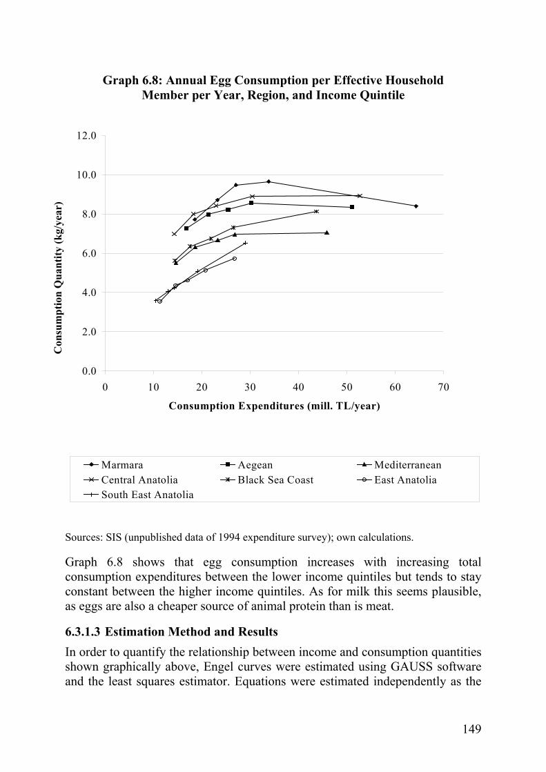
149

Graph 6.8: Annual Egg Consumption per Effective Household Member per Year, Region, and Income Quintile

Sources: SIS (unpublished data of 1994 expenditure survey); own calculations.

Graph 6.8 shows that egg consumption increases with increasing total consumption expenditures between the lower income quintiles but tends to stay constant between the higher income quintiles. As for milk this seems plausible, as eggs are also a cheaper source of animal protein than is meat.

6.3.1.3 Estimation Method and Results In order to quantify the relationship between income and consumption quantities shown graphically above, Engel curves were estimated using GAUSS software and the least squares estimator. Equations were estimated independently as the

0.0

2.0

4.0

6.0

8.0

10.0

12.0

0 10 20 30 40 50 60 70

Consumption Expenditures (mill. TL/year)

Con

sum

ptio

n Q

uant

ity (k

g/ye

ar)

Marmara Aegean MediterraneanCentral Anatolia Black Sea Coast East AnatoliaSouth East Anatolia

150

adding up condition could not be applied due to limited product coverage, and consumption quantity, not expenditure, as the dependent variable. The functional form applied in all but one case is the half-logarithmic form as it well depicts the expected and observed pattern of falling income elasticities with increasing income. Alternatively, the linear and double logarithmic forms have been tested. In two cases, the double logarithmic form performed slightly better than the half-logarithmic form in terms of R-square, and in three cases it performed better with respect to nonspherical disturbances. Nonetheless, results of the half-logarithmic form were chosen for their better consistency with theory. Regional level dummies (D1-D6) were included in order to depict regional differences in consumption patterns previously described in Section 6.3.1.2. Regional level dummies with t-values below unity were removed.

No regional slope dummies were included because degrees of freedom are very limited. In addition, data mainly displays level differences among regions and slight differences in slope. Also differences in slope among regions is not of great interest, as in this study national income elasticities are needed because human demand is modeled at the national level. Including slope dummies would result in differences of income elasticities among regions, and the calculation of a national average income elasticity would then be required. Without slope dummies, this "averaging" procedure is performed by the least squares estimator.

The statistical model for estimation is:

(6.8) qt = α + γ1 • D1 + γ2 • D2 + γ3 • D3 + γ4 • D4 + γ5 • D5 + γ6 • D6 + β • ln ext + εt.

For wheat consumption, the linear form was chosen in order to depict the consumption pattern described above. For this purpose two linear equations were estimated, one based upon data of income quintiles one and two, and one based on income quintiles two to five. The statistical model in that case is

(6.9) qt = α + γ1 • D1 + γ2 • D2 + γ3 • D3 + γ4 • D4 + γ5 • D5 + γ6 • D6 + β • ext + εt.

Results of estimations are presented in Table 6.6 below.The explanatory power of the chosen model is high: all adjusted R-squares are above 0.83 and F-values

151

are high. Except for sunflower seed oil, all slope parameters are significant at one percent level.51

Table 6.6: Results of Estimation of Engel Curves Wheat1 Wheat2 Sunoil Ol. oil Beef Sheep Poultry Milk Eggs

Functional form

linear linear h.-log h.-log h.-log h.-log h.-log h.-log h.-log

Constant (α) (t-value)

11.112 (12.3)

17.192 (52.8)

1.797 (3.6)

-0.705 (3.0)

-5.866(10.7)

-3.161(6.4)

-3.418 (12.2)

-36.86 (6.0)

-1.156(4.1)

Slope variable (β)

0.194 -0.111 -0.043 0.055 0.485 0.224 0.265 3.238 0.127

(t-value) (3.9) (8.8) (1.4) (3.4) (13.0) (6.6) (14.0) (7.6) (6.6) ** ** ** ** ** ** ** **

Degrees of freedom

6 25 29 27 27 28 27 28 28

Adj. R2 0.97 0.84 0.95 0.85 0.96 0.86 0.93 0.83 0.91

F 63.6 72.1 120.0 28.1 109.4 35.5 70.1 29.5 56.8 ** = significant at 1 percent level. Source: Own estimates.

Based on the estimation results of slope parameters, elasticities of demand with respect to total expenditure are calculated for each income quintile according to

(6.10) ηq, ex= β/ex for the half-logarithmic cases,

and

(6.11) ηq, ex= β • ex/q in the case of wheat elasticities,

51 Autocorrelation and heteroskedasticity was tested for and results are heterogeneous. Due to low degrees of freedom the Durbin-Watson test is inconclusive at five percent significance level in eight out of nine cases, and in one case the null hypothesis of no autocorrelation is rejected. Therefore the Breusch and Godfrey test on autocorrelation is also applied. Due to the limited number of observations, only up to third degree autocorrelation is tested for and cannot be rejected in five out of nine observations at five percent significance level. Heteroskedasticity can not be rejected at 5 percent significance level in three out of nine cases according to the White test. Notwithstanding these results, parameters are used for calculation of elasticities as underlying data is considered the best available basis and limited degrees of freedom do not allow to correct for autocorrelation and heteroscedasticity.

152

with ex being the regional average of total expenditure per effective household member in the respective income quintile.

No elasticities are calculated for sunflower seed oil as estimated slope parameters, in the half-logarithmic as well as the linear form, are close to zero and not significant. The resulting elasticities are presented in Table 6.7

Table 6.7: Elasticities of Demand with Respect to Total Expenditures, Estimation Results

Quintile 1 Quintile 2 Quintile 3 Quintile 4 Quintile 5

Wheat 0.09 -0.08 -0.14 -0.18 -0.38

Olive oil 0.39 0.35 0.33 0.31 0.26

Beef 0.80 0.67 0.59 0.52 0.39

Sheep meat 0.94 0.76 0.65 0.57 0.42

Poultry meat 1.26 0.96 0.80 0.67 0.48

Milk 0.32 0.29 0.28 0.26 0.22

Eggs 0.23 0.22 0.20 0.19 0.18 Source: Own calculations.

Income elasticities reach from -0.38 for the upper income quintile for wheat and around unity for meat in lower income quintiles. Due to the high share of wheat in the Turkish diet and the high protection level for this product, the low demand elasticity found for wheat is of special empirical relevance. Also the fact that sunflower seed oil consumption was found to be independent of income is an interesting result which contrasts with other empirical studies (KOC et al., 1998). It seems plausible, however, if one takes into account that with increasing income it is mainly consumption of more expensive fats (olive oil and butter) which increases.

6.3.2 Development of Elasticity Matrices of Human Demand for Each Income Quintile

A matrix of compensated price elasticities of human demand for all products covered by TURKSIM with respect to all prices of products covered by TURKSIM and the price for other products is built. This matrix fulfils the conditions of symmetry and adding up locally, and the condition of homogeneity of degree zero in all prices globally. The elasticities of demand with respect to the price for the aggregate of other products do not enter TURKSIM but are necessary to ensure the fulfilment of the conditions of homogeneity and adding up. Income, own and cross price elasticities of demand in TURKSIM are

153

derived according to the following steps, which are explained in more detail below.

1. Income and own price elasticities of demand (el_inci,inc and el_hdi,inc) for each income quintile (inc) are determined on the basis of own estimates, literature, expert interviews, and plausibility considerations.

2. Products are classified into groups of more or less close substitutes in consumption.

3. Allen elasticities of substitution (σi,j), which are measures for the degree of technical substitutability of products independent of their current budget shares, are determined simultaneously for each pair of products based on the classification in (2) above. The determination of Allen elasticities is restricted by the homogeneity condition of demand:

(6.11) el_inci,inc + ∑j (el_hdi, j,inc ) = 0, or

(6.12) ∑j (el_hd_ci, j,inc ) = 0

with el_hd_c being the compensated price elasticities of demand. In order to take into account the homogeneity condition in the selection of Allen elasticities, compensated cross price elasticities for one of the quintiles are derived from Allen-elasticities according to

(6.13) el_hd_ci, j,inc = σi, j • vj,inc,

with vj being the value share of product j in quintile inc.

4. The resulting Allen elasticities are then transformed into compensated cross price elasticities for the other four income quintiles by multiplication with the respective value shares.

5. In case of the homogeneity condition (6.11) being hurt, all Allen elasticities for the respective quintile and product are scaled down or up uniformly in relative terms.

6.3.2.1 Determination of Income and Own Price Elasticities Table 6.8 presents the income elasticities used in TURKSIM for all income quintiles as well as the national average and the sources used.

154

Table 6.8: Income Elasticities in TURKSIM Quin1 Quin2 Quin3 Quin4 Quin5 Nat. Source Common wheat 0.09 -0.08 -0.14 -0.18 -0.38 -0.15 Own estimate Durum wheat 0.09 -0.08 -0.14 -0.18 -0.38 -0.15 Own estimate Barley 0.94 0.76 0.65 0.57 0.42 0.65 As sheep meat Maize 0.09 -0.08 -0.14 -0.18 -0.38 -0.15 As wheat Chickpeas 0.09 -0.08 -0.14 -0.18 -0.38 -0.15 As wheat Dry beans 0.09 -0.08 -0.14 -0.18 -0.38 -0.15 As wheat Lentils 0.09 -0.08 -0.14 -0.18 -0.38 -0.15 As wheat Tobacco 1.03 0.84 0.72 0.63 0.46 0.72 1.1 * sheep meat (KOC et al.) Sugar 0.28 0.23 0.20 0.17 0.13 0.20 0.3 * sheep meat (KOC et al.) Cotton Sunflower seed 0.28 0.23 0.20 0.17 0.13 0.20 0.3 * sheep meat Soybeans Onions 0.28 0.23 0.20 0.17 0.13 0.20 0.3 * sheep meat Potatoes 0.09 -0.08 -0.14 -0.18 -0.38 -0.15 As wheat Table tomatoes 0.56 0.46 0.39 0.34 0.25 0.39 0.6 * sheep (KOC et al.) Tomato paste 0.56 0.46 0.39 0.34 0.25 0.39 0.6 * sheep (KOC et al.) Melon 0.56 0.46 0.39 0.34 0.25 0.39 0.6 * sheep (KOC et al.) Cucumbers 0.56 0.46 0.39 0.34 0.25 0.39 0.6 * sheep (KOC et al.) Peppers 0.56 0.46 0.39 0.34 0.25 0.39 0.6 * sheep (KOC et al.) Apples 0.56 0.46 0.39 0.34 0.25 0.39 0.6 * sheep (KOC et al.) Table olives 0.56 0.46 0.39 0.34 0.25 0.39 0.6 * sheep (KOC et al.) Olive oil 0.39 0.35 0.33 0.31 0.26 0.32 Own estimate Lemons 0.56 0.46 0.39 0.34 0.25 0.39 0.6 * sheep (KOC et al.) Oranges 0.56 0.46 0.39 0.34 0.25 0.39 0.6 * sheep (KOC et al.) Mandarins 0.56 0.46 0.39 0.34 0.25 0.39 0.6 * sheep (KOC et al.) Hazelnuts 0.75 0.61 0.52 0.46 0.34 0.52 0.8 * sheep Table grapes 0.56 0.46 0.39 0.34 0.25 0.39 0.6 * sheep (KOC et al.) Sultanas 0.56 0.46 0.39 0.34 0.25 0.39 0.6 * sheep (KOC et al.) Tea 0.56 0.46 0.39 0.34 0.25 0.39 0.6 * sheep (KOC et al.) Milk 0.32 0.29 0.28 0.26 0.22 0.27 Own estimate Sheep meat 0.94 0.76 0.65 0.57 0.42 0.65 Own estimate Beef 0.80 0.67 0.59 0.52 0.39 0.58 Own estimate Poultry 1.25 0.96 0.79 0.67 0.45 0.80 Own estimate Eggs 0.23 0.22 0.21 0.20 0.18 0.20 Own estimate Sunflower oil 0.00 0.00 0.00 0.00 0.00 0.00 Own estimate Sunflower cake Soybean oil 0.00 0.00 0.00 0.00 0.00 0.00 As sunflower oil Soy cake - Cotton lint 1.25 0.96 0.79 0.67 0.45 0.80 As poultrymeat (SWOPSIM) Cottonseed - Cotton oil 0.00 0.00 0.00 0.00 0.00 0.00 As sunflower oil Cottonseed cake - Other 1.81 1.70 1.57 1.45 1.26 1.54 Residual acc. to adding up Sources: Own calculations; KOC et al. (1998); USDA (2002).

155

For some products, income elasticities used in TURKSIM are based on own estimates, e.g. wheat and animal products. Some other products are considered to be similar with respect to their relative superiority and therefore similar elasticities are applied. This is the case, for example, for pulses and potatoes, which are low income, basic food commodities and are therefore considered to be subject to the same income elasticities; or for barley, which for human consumption is used mainly for beer production and is therefore considered to be subject to income elasticities higher than for basic food commodities. The degree of "luxuriousness" of barley was therefore assumed to be as high as that of sheep meat. For some products, estimates from other analyses are taken into account. In those cases results are often taken in relation to products for which own estimates are available. This is because estimates from other analyses usually include the quality component not included in own estimates. For example, the income elasticity of for sheep meat demand is as high as the one for poultry according to the SWOPSIM database, and the income elasticity for tobacco is somewhat higher than the one for sheep meat according to KOC et al. (1998). The income elasticity for the aggregate of other products is a residual which is determined based on the adding up restriction:

(6.14) ∑i el_inci,inc • vi,inc = 1.

This does not enter TURKSIM, but is calculated as a consistency check. The aggregate "other products" includes agricultural products not covered by this analysis as well as the quality component of the products covered, and all nonagricultural products like housing and clothes. All in all, this product group is a luxury with an income elasticity above Unity for all income quintiles, whereas the agricultural products included are, on aggregate, a necessity.

Own price elasticities in TURKSIM are determined according to the following steps.

1. A national average, uncompensated, own price elasticity is chosen based on literature, expert interviews, and plausibility considerations. This is chosen as a first step, as uncompensated own price elasticities are reported in most published results of econometric analyses and are easiest to grasp intuitively. Plausibility considerations are based mainly on the estimated degree of substitutability (products which can be expected to be substituted easily are assumed to have a high own price elasticity) and the level of the income elasticity (products with a high income elasticity are expected to be subject to a relatively high own price elasticity, too).

2. An Allen elasticity of substitution is calculated from this own price elasticity according to

156

(6.15) σi, i = (el_hdi, i +vi•el_inci)/vi .

3. Allen elasticities of substitution are assumed to be equal for all income quintiles, and compensated own price elasticities are calculated for each quintile by dividing σi, j by the respective value share (vj,inc).52 The implicit assumption is that technical substitutability does not depend on income level, an assumption which may be questioned; but no additional information was available.

The determination of uncompensated own price elasticities was based on KOC et al. (1998) and, in a few cases, BROSIG (2000) and the SWOPSIM database. Table 6.9 presents an overview of the resulting own price elasticities.

52 Later this assumption was somewhat relaxed in order to fulfill the homogeneity condition.

157

Table 6.9: Own Price Elasticities in TURKSIM Compensated Uncompensated

Quin1 Quin2 Quin3 Quin4 Quin5 National National Common wheat -0.17 -0.16 -0.13 -0.12 -0.06 -0.11 -0.10 Durum wheat -0.16 -0.15 -0.13 -0.11 -0.06 -0.10 -0.10 Barley -1.01 -1.09 -1.14 -1.13 -0.97 -1.00 -1.00 Maize -0.16 -0.15 -0.13 -0.11 -0.06 -0.10 -0.10 Chickpeas -0.16 -0.15 -0.13 -0.11 -0.06 -0.10 -0.10 Dry beans -0.16 -0.15 -0.13 -0.11 -0.06 -0.10 -0.10 Lentils -0.16 -0.15 -0.13 -0.11 -0.06 -0.10 -0.10 Tobacco -1.01 -1.08 -1.13 -1.12 -0.97 -1.00 -1.00 Sugar -0.19 -0.18 -0.17 -0.15 -0.10 -0.14 -0.14 Cotton Sunflower seed -0.70 -0.65 -0.61 -0.55 -0.37 -0.50 -0.50 Soybeans Onions -0.28 -0.26 -0.24 -0.22 -0.15 -0.20 -0.20 Potatoes -0.33 -0.30 -0.26 -0.22 -0.12 -0.20 -0.20 Table tomatoes -1.22 -1.19 -1.17 -1.10 -0.83 -0.99 -1.00 Tomato paste -1.23 -1.20 -1.18 -1.11 -0.84 -1.00 -1.00 Melon -1.23 -1.20 -1.17 -1.10 -0.84 -0.99 -1.00 Cucumbers -1.23 -1.20 -1.18 -1.11 -0.84 -1.00 -1.00 Peppers -1.23 -1.20 -1.18 -1.11 -0.84 -1.00 -1.00 Apples -1.23 -1.20 -1.17 -1.11 -0.84 -1.00 -1.00 Table olives -1.23 -1.20 -1.18 -1.11 -0.84 -1.00 -1.00 Olive oil -1.28 -1.06 -1.31 -1.09 -0.83 -1.00 -1.00 Lemons -0.62 -0.60 -0.59 -0.55 -0.42 -0.50 -0.50 Oranges -1.23 -1.20 -1.18 -1.11 -0.84 -1.00 -1.00 Mandarins -1.23 -1.20 -1.18 -1.11 -0.84 -1.00 -1.00 Hazelnuts -1.23 -1.20 -1.17 -1.11 -0.84 -1.00 -1.00 Table grapes -1.23 -1.20 -1.17 -1.10 -0.84 -0.99 -1.00 Sultanas -1.24 -1.21 -1.18 -1.11 -0.84 -1.00 -1.00 Tea -0.61 -0.60 -0.59 -0.55 -0.42 -0.50 -0.50 Milk -0.49 -0.49 -0.48 -0.42 -0.29 -0.38 -0.40 Sheep meat -1.18 -1.27 -1.33 -1.32 -1.13 -1.17 -1.18 Beef -1.08 -1.23 -1.39 -1.34 -1.15 -1.17 -1.18 Poultry -0.99 -1.15 -1.36 -1.43 -1.16 -1.17 -1.18 Eggs -0.65 -0.65 -0.62 -0.57 -0.34 -0.49 -0.49 Sunflower oil -0.73 -0.64 -0.58 -0.50 -0.30 -0.47 -0.47 Sunflower cake Soybean oil -1.13 -0.99 -0.89 -0.78 -0.47 -0.72 -0.72 Soy cake Cotton lint -0.16 -0.18 -0.22 -0.23 -0.18 -0.19 -0.20 Cottonseed Cotton oil -1.13 -0.99 -0.89 -0.78 -0.47 -0.72 -0.72 Cottonseed cake Other -0.18 -0.20 -0.20 -0.21 -0.23 -0.23 -1.20 Sources: KOC et al. (1998); USDA (2002); BROSIG (2000); own calculations.

158

6.3.2.2 Determination of Cross Price Elasticities For the determination of Allen elasticities of substitution, products were at first grouped in more or less close substitutes. The full table of Allen elasticities is presented in Table A-6.21 of the Annex. Only the upper triangle of the product matrix is filled, as Allen-elasticities are symmetric. Carbohydrate products like cereals, potatoes, and, to a lesser degree, sugar, are assumed to be substitutes. Within the fruit and vegetable groups, substitutability is assumed to be high as well. Strong substitutability also exists between red meats and, to a lesser extent, poultry and other sources of animal protein. Also oils and, to a lesser extent, milk are assumed to be substitutes. The Allen elasticities of substitution are set between zero (for many products, for example cereals and vegetables) and 30 (for example cottonseed oil and sunflower seed oil). Their total size is restricted by the homogeneity condition, i.e. when a product is considered a better substitute for some product, some other product must be a less good substitute.

Resulting cross price elasticities vary between zero and 0.73 for tomato paste with respect to the table tomato price in income quintile 1. The full matrices of compensated price elasticities of demand per income quintile are presented in Tables A-6.22-26 of the Annex. Only cross price elasticities exceeding the absolute value of 0.05 are included in the tables.

6.3.3 Development of Elasticity Matrices of Feed Demand

Results of empirical work on price dependency of demand for feed components are very heterogeneous (PEETERS and SURRY, 1997) and, for Turkey, rather limited (FULLER et al., 1999). FULLER et al. estimate feed component demand functions for Turkish milk and meat production derived from a translog cost function. Unfortunately, formula feed is included as a single aggregate which results in estimates of limited use for this study in which components of formula feed are analyzed separately. Helpful, however, is the estimation of own price elasticities for forage, which is excluded from most other studies on feed demand. The own price elasticities for forage are found to lie between –0.63 for cow milk production and –0.84 for sheep meat production. Various econometric estimations of feed demand (SURRY, 1990, 1993; PEETERS and SURRY 1994) report compensated price elasticities of feed demand between –0.3 and –3.3 for cereals, -0.37 and –0.57 for soybean meal, and –0.37 and –0.96 for other protein components. For this study compensated own price elasticities of feed demand are assumed to lie between –0.38 and –1.5 for cereals, between –0.56 and –1.13 for oilseeds and pulses, and –0.4 and –0.65 for coarse feed. The own price elasticity for milk as feed for ruminants is considered to be extremely low (-0.01) as almost no possibilities for substitution exist.

159

Cross price elasticities are determined by grouping products into more or less close substitutes and choosing symmetric Allen-elasticities of substitution which are then transformed into compensated cross price elasticities subject to the homogeneity condition. Feed demand per unit of output is homogeneous of degree zero in component prices: If all prices vary by the same relative magnitude, feed composition does not change. In order to properly apply the homogeneity condition, coarse feed, not included in TURKSIM, is included in the elasticity matrices. This is because coarse feed is a clear substitute for other feed components, and the implementation of the homogeneity condition without considering coarse feed would overestimate the size of cross price elasticities for other substitutes.

The resulting Allen elasticities, which lie between zero and 10.2 in the case of lentils and chickpeas in sheep meat production, are presented in Tables A-6.27 to A-6.31 of the Annex. The resulting cross price elasticities, between zero and 1.13 in the case of cereals with respect to coarse feed in milk production, are presented in Tables A-6.32 to A-6.36 of the Annex.

6.3.4 Determination of Processing Demand Elasticities

As processing activities are modeled only rudimentarily without explicitly depicting the dependency of the amount of processing on the relative and the absolute processing margin (see Subchapter 5.5), elasticities are set relatively low in order to avoid a strong influence of changing prices on the degree of domestic processing. This may also be adequate, as TURKSIM is used for midterm projections whereas the amount of domestic processing strongly depends on long term investments. For TURKSIM, the elasticity of processing demand with respect to total cost is assumed to be -0.5 for all oil crushing industries. As processing demand is assumed to be homogeneous of degree zero in all prices and, in a competitive industry, profit does not exist, the elasticity of processing demand with respect to all output prices must therefore be 0.5. In order to calculate elasticities with respect to individual input and output prices, cost and revenue for each processing industry has been decomposed, as shown in Table 6.10 for the sunflower seed crushing industry. Row 2 of Table 6.10 presents prices for the input (sunflower seed) and the outputs (cake and oil) as used for the calibration of TURKSIM in the base period. Row 3 shows the physical input and output shares of the respective products as used in TURKSIM and taken from the FAO supply utilization accounts. Row 4 presents the value per ton of seed processed as the price per ton multiplied by the physical share. The amount of other cost (Column 5, Row 4) is calculated by deduction of seed cost (82.23) from total revenue (10.01 + 82.84). The value shares (Row 5) are then calculated by expressing seed and other cost as shares in total cost (with a negative sign) and by expressing cake and oil revenue as shares in total revenue.

160

The processing demand elasticities (Row 6) are calculated by multiplying the respective value shares by 0.5 and only the elasticities of Columns 2 to 4 are used in TURKSIM as other cost is not explicitly modeled.

Table 6.10: Calculation of Processing Demand Elasticities of the Sunflower Seed Crushing Industry

1 2 3 4 5

1 Seed Cake Oil Other cost

2 Price (mill. TL/t) 82.23 22.44 220.32

3 Physical share 1 0.446 0.376

4 Value (2 • 3) 82.23 10.01 82.84 10.62

5 Value share -88.6% 10.8% 89.2% -11.4%

6 Elasticity (value share • 0.5) -0.44 0.05 0.45 -0.06 Sources: FAO (2002a); own calculations.

Processing demand elasticities for all three crushing industries are presented in Table 6.11.

Table 6.11: Processing Demand Elasticities Seed Cake Oil

Sunflower seed -0.44 0.05 0.45

Cottonseed -0.35 0.15 0.35

Soybeans -0.45 0.20 0.30 Source: Own calculations.

6.4 Estimation of Price Transmission Elasticities for Animal Products

Turkey has been a significant importer of two animal products in recent years: milk and beef. For these products, a time series of duty paid border prices and domestic prices has been generated in order to check the working hypothesis that changes in the duty paid import price are not fully transmitted to the internal price.

Turkey has been an importer of beef since 1985 when trade barriers were lowered, until 1996. In 1997, an import ban came into effect and prohibited significant imports. From 1985 to 1996 imports covered between 3 and 15 percent of domestic consumption. For this period, a price series of import prices was calculated from Turkish import statistics. For 1989 to 1996, import unit values of frozen compensated beef quarters were taken as indicators for the average import price, as significant quantities of this product were imported in each of these years. For the years 1985 through 1988, import unit values for

161

fresh meat of bovine animals were taken, as no significant quantities of frozen quarters were traded. This approach is justified by the fact that the unit value for the two products were reasonably close in the years 1989 to 1991. Table 6.12 presents price data for beef.

Table 6.12: Turkish Import, Border, and Domestic Prices for Beef (US$/t)

1985 1986 1987 1988 1989 1990 1991 1992 1993 1994 1995 1996

Im. price (unit value)

1,108 958 1,216 1,016 871 1,458 1,275 1,010 967 1,046 1,666 1,325

Ad valorem tariff

1% 1% 1% 1% 1% 1% 1% 1% 15% 15% 15% 105%

Specific tariff

50 250 400 400 600 600 900 1,300 1,500 1,500 1,000

Transport margin

47 47 47 47 47 47 47 47 47 47 47 47

Border price

1,216 1,265 1,675 1,473 1,527 2,120 2,235 2,367 2,659 2,750 2,963 2,763

Farmgate price

1,183 1,495 2,157 1,894 2,105 2,933 3,264 3,510 3,572 2,424 3,913 3,077

Wholesale margin

305 305 305 305 305 305 305 305 305 305 305 305

Wholesale price

1,488 1,800 2,462 2,199 2,410 3,238 3,569 3,815 3,877 2,729 4,218 3,382

Sources: SIS (import statistics); UFT (tariffs); OECD (farmgate price); own calculations.

Tariffs and a transportation margin (as applied in TURKSIM) are added to the import price in order to generate a duty paid border price at wholesale level to be compared to the internal price, which is generated by adding a wholesale margin (as applied in TURKSIM) to the OECD reported farmgate price.53 The border price and the internal wholesale price are presented graphically in Graph 6.9.

53 There is no reason, of course, to assume that such a margin should stay constant over time. No empirical information, however, on the development of such a margin was available.

162

Graph 6.9: Turkish Border and Internal Wholesale Prices for Beef, 1985-1996 (US$/t)

Sources: Various sources (see below); own calculations.

Graph 6.9 shows that the internal price usually lies above the border price and follows, to a certain extent, the movement of the border price. This positive price correlation can especially be observed, independently of the overall trend of increasing beef prices, in the years 1987 to 1990 and 1995 to 1996, when prices deviate from the overall increasing trend. The 1994 internal price is distorted due to a strong devaluation of the Turkish Lira in 1994, so 1994 is not included in the data set for estimation.

The years 1990 to 2000 were a period of dairy product imports exceeding one percent of raw milk equivalent of domestic milk consumption in most years. A price series of duty paid border prices was created for this period using Turkish import unit values for SMP (CN position 04021019) and butter (CN position 04050011) as indicators for the average price level of imported dairy products. The results are presented in Table 6.13. The tariff-paid border prices for butter and SMP are aggregated by weighting them with their relative extraction factors, and a transportation margin is added as applied in TURKSIM in order to create a border price per ton of raw milk equivalent at wholesale level. A processing margin as applied in TURKSIM is added to the farmgate price in order to create an internal price at wholesale level for comparison to the border price. The

0

500

1,000

1,500

2,000

2,500

3,000

3,500

4,000

4,500

1985 1986 1987 1988 1989 1990 1991 1992 1993 1994 1995 1996

Year

US$

/t Border PriceInternal Price

163

processing margin is rather large and even exceeds the farmgate price in one year. This wholesale margin was calculated for the base period of TURKSIM (see Subchapter 7.2 below); for the purpose of this analysis it is assumed to be constant in dollar terms over the period 1990 to 2000. Therefore the internal price at wholesale level could be distorted, as the reasons for such a high margin and its development over time are obscure. An alternative would be the direct use of observed, internal SMP and butter wholesale prices. This approach, however, has not been followed as SMP prices in Turkey are neither collected nor published. Rather TURKSIM base period data were collected from individual companies (see Subchapter 7.2).

Table 6.13: Turkish Import, Border, and Domestic Prices for Dairy Products (US$/t)

1990 1991 1992 1993 1994 1995 1996 1997 1998 1999 2000

Im. price butter 1,291 814 921 1,193 1,435 1,902 1,962 1,756 2,003 1,669 1,687

Ad valorem tariff butter

30% 30% 30% 5% 5% 5% 50% 70% 70% 70% 100%

Sp. tariff butter 400 400 400 900 900 500

Tariff paid border price butter

2,078 1,458 1,597 2,153 2,407 2,497 2,943 2,985 3,405 2,837 3,374

Import price SMP 879 813 1,269 1,577 1,384 1,746 1,805 1,752 1,656 1,351 1,556

Ad val. tariff SMP 1% 1% 1% 26% 20% 20% 75% 130% 130% 130% 150%

Sp. tariff SMP 700 1,000 1,200 1,200 1,300 1,300 30

Tariff paid border price SMP

1,588 1,821 2,482 3,187 2,961 3,395 3,189 4,030 3,809 3,107 3,890

Transport margin 24 24 24 24 24 24 24 24 24 24 24

Weighted border price

259 253 320 408 399 442 443 522 520 431 526

Farmgate price 285 274 306 286 223 283 317 359 341 275 264

Wholesale margin 246 246 246 246 246 246 246 246 246 246 246

Wholesale price 531 520 552 532 469 529 563 605 587 521 510Sources: SIS (import statistics); UFT (tariffs); OECD (farmgate price); own calculations.

The border price and the internal wholesale price are presented graphically in Graph 6.10. Graph 6.10 shows that the internal price is above the border price for the whole period, except for the year 2000. The correlation, however, is less clear than in the case of beef. During periods 1992 to 1993 and 1999 to 2000 prices, move in opposite directions, whereas correlation is positive in other periods.

164

Graph 6.10: Border Price and Internal Wholesale Price for Milk, 1989-2000 (US$/t)

Sources: Various sources (see below); own calculations.

In order to quantify the relationship between the internal price and the border price the following statistical model was estimated in GAUSS using the least squares estimator.

(6.16) ln PIt = α + β • ln PBt + γ • t + εt,

with PI being the internal price, PB being the border price and t being the respective year. The trend parameter γ is included as a simple approach to account for the nonstationarity of price series. β is the price transmission elasticity of the internal price with respect to the border price. Estimation results are presented in Table 6.14. In the case of beef, the price transmission elasticity is estimated at 0.66, significant at a 5 percent level. The explanatory value of the chosen model is high, as the adjusted R-square is at 0.93 and the F-value is at 69. The Durbin Watson test is inconclusive but the Breusch and Godfrey test for autocorrelation rejects first order autocorrelation at the five percent significance level. The result is in accordance with a priori assumptions that domestic prices are linked to border prices, but price transmission is not complete. Price transmission elasticities for meat in TURKSIM are therefore set at 0.66.

0

100

200

300

400

500

600

700

1990 1991 1992 1993 1994 1995 1996 1997 1998 1999 2000

Year

US$

/t Border PriceInternal Price

165

Table 6.14: Estimation of Price Transmission Elasticities for Beef and Milk

Beef Milk

Functional form log-linear log-linear

Period covered 1985-1996 excl. 1994 1993-1999

Degrees of freedom 8 4

Constant 2.696 1.459 (t-value) (1.7) (1.1)

Price transmission elasticity 0.657 0.796 (t-value) (2.8) (3.4) * *

Trend parameter 0.169 -0.02

(t-value) (1.7) (0.6)

Adj. R2 0.931 0.708

F 68.7 8.3 * = significant at 5 percent level. Source: Own estimates.

In the case of milk, no significant results are obtained from full period data 1990 to 2000. If, however, periods 1990-1993 and 1999-2000 are excluded, the resulting price transmission elasticity is at 0.8 and significant at five percent, and first order autocorrelation is rejected by the Durbin Watson as well as the Breusch and Godfrey tests. The exclusion of 1999-2000 can be justified by the sudden devaluation of the Turkish Lira, but not so the exclusion the period 1990-1993. Nonetheless the price transmission elasticity for milk and eggs in TURKSIM is set at 0.8. This is because no better a priori assumption exists and it seems plausible that price transmission for milk products and eggs is somewhat higher than that for meat due to lower transportation cost for these products (e.g. in the form of SMP or dried eggs).

167

7 DATA SET FOR MODEL CALIBRATION

The base period for TURKSIM with respect to the quantitative framework (yield, area, supply, trade, and demand) is the average of the years 1997 through 1999 for plant products and the average of the years 1998 through 1999 for animal products. A two year average is considered sufficient for animal products; animal production is much less volatile than plant production as it depends less on climatic conditions of the respective year. For prices, wholesale as well as farmgate, and the relevant price margins, the average of the years 1996/98 was chosen in order to make allowance for some lagged adjustment at the supply side, which is of course more distinct in animal production due to the respective production cycles and long-term investment decisions. For some products the base period was adjusted for specific reasons which are explained below in the respective sections.

7.1 Supply, Trade, and Demand

7.1.1 Supply

7.1.1.1 Standard Approach Area and yield of plant products and supply of animal products are taken from Agricultural Structure yearbooks (SIS, various issues) for 81 provinces and data is aggregated at the level of nine agricultural regions (sum for area and supply; area weighted average for yield). In some cases, when published data include obvious errors of data collection or processing, adjustments are made based on plausibility considerations. Resulting national totals are checked for consistentcy with published national data. Annex Table A-7.1 presents base yield, area, and supply for all regions as well as national totals. For the processing outputs supply is based on Agricultural Structure for cotton lint and cottonseed and on FAO commodity balances (FAO, 2002a, b) for oils and oil cakes.

7.1.1.2 Specific Cases Vegetables: SIS publishes production quantities of vegetables, but not product specific area and yield data. Product-specific area data is obtained by SIS on a national level but is not available at regional level. In order to depict regional competition for area with crops and fruit in TURKSIM, regional area and yield data is generated by calculating national yield data from national area and production quantities, and assuming yield to be similar across regions. Regional area is calculated from regional quantity data divided by national yield data.

Fruit: For fruit, SIS publishes only numbers of trees and supply quantities, not area and yield data. Estimates of the national average number of trees per ha are

168

obtained from MARA and are assumed to be similar across regions. Table 7.1 shows the number of trees per ha.

Table 7.1: Number of Fruit Trees Product Number of trees/ha

Olives

Oranges, lemons, mandarins

Apples

Hazelnuts

100

300

150

300 Source: Interviews at MARA.

In order to consider competition for area with crops and vegetables in TURKSIM, product specific regional area and yield data is calculated by dividing the regional number of trees by the average national number of trees per ha and by dividing the regional production quantity by the resulting regional area.

Durum wheat: Area and yield data for wheat are published by SIS for total wheat, including common and durum wheat. Based on interviews with officials of the Turkish Grain Board, the assumption is made that 20 percent of Turkey's total wheat area is allocated to durum wheat uniformly across all regions, and yield is assumed to be as high for durum as for common wheat.

Sugar: Sugar beet yield reported by SIS is transformed into sugar using an extraction factor of 12 percent based on FAO (2002b).

Tomato paste: Production of tomato paste is not published by SIS. Production data therefore comes from USDA (various issues) and is broadly in line with data published by TOMATO NEWS (2002). 22,000 tons of estimated home production are added to the USDA data (TOMATO NEWS 10/94). As shown in Table 7.2 tomato paste production is highly volatile.

169

Table 7.2: Tomato Paste Production Quantities and Prices, 1997-2001 1997 1998 1999 2000 2001

USDA production estimate (tons) 185,000 310,000 320,000 265,000 170,000

Estimated home production 22,000 22,000 22,000 22,000 22,000

Total 207,000 332,000 342,000 287,000 192,000 Sources: Tomato News (1994); USDA (GAIN Reports, various issues); own calculations.

As the average of tomato paste production in the TURKSIM base period 1997 to 1999 is close to the average of the longer period 1997 to 2001, it is taken as base quantity for TURKSIM. The yield of paste tomatoes is assumed to equal the yield of table tomatoes and the area for paste tomatoes is calculated by assuming an extraction factor of 1 kg paste out of 5.5 kg tomatoes, which is reported by USDA (various issues). 80 percent of tomato paste area is allocated to the Aegean agricultural region (USDA GAIN Report TU1028, 19.05.2001, p. 2). The other 20 percent are allocated to the other regions according to their shares in total tomato area. The regional area for table tomatoes is calculated as the residual of total regional tomato area minus the area for paste production.

Olive oil: Production of olive oil is not published by SIS. Production data therefore comes from the IOOC (2002) and is broadly in line with data published by USDA (various issues). Due to the high volatility of production (see Table 7.3) a four year average of the years 1997 to 2000 is used for calibration of production (as well as consumption and trade) in TURKSIM.

Table 7.3: Olive Oil Production Quantities, 1997-2001 1997 1998 1999 2000 Av. 97/00 2001

IOOC production estimate (tons, marketing year)

40,000 170,000 70,000 190,000 117,500 60,000

Sources: IOOC (2002); own calculations.

The yield of olives for oil is assumed to equal the yield of table olives, and the area for olive oil is calculated by assuming an extraction factor of 1 kg oil out of 6 kg olives. FAO (2002b) reports an extraction factor of 7 in its commodity balances, but experts from the industry in Turkey report a factor of 5. National area for oil olives is allocated to regions according to their area shares in total olive area. The regional area for table olives is calculated as the residual of total regional olive area minus the area for oil production.

Sultanas: Production of sultanas is not published by SIS. Production data therefore comes

170

from GAIN Reports of the USDA (various issues). Due to data availability an average of the years 1999 to 2000 was taken for calibration. The yield of sultana grapes is assumed to equal the yield of table grapes and the area for sultana grapes is calculated by assuming an extraction factor of 1 kg sultanas out of 4.5 kg grapes. National area for sultanas is allocated completely to the Aegean region.54

Red meat: Data published by SIS for red meat underestimates total production as only data of municipal slaughterhouses and estimates for slaughtering for religious festivals are included. This underestimation is especially significant in the case of sheep meat, for which more than half of total production falls outside the SIS statistics. Therefore FAO (2002a) estimates of total production are used. Indigenous meat production is calculated by adding the meat equivalent of live animals exported minus the meat equivalent of live animals imported. Production is allocated to agricultural regions by applying the shares resulting from provincial production data reported by SIS.

Poultry and eggs: For poultry meat and eggs estimates of BESD-BIR, the Association of Turkish Poultry Producers are used, which are about 20 percent above official data for poultry and about 20 percent below official data for eggs. Production is allocated to agricultural regions by applying the shares resulting from SIS reported provincial production data.

7.1.2 Trade

Trade data is for the same period as production data and is taken from FAO and identical with the data provided from SIS. For a few products trade data is directly taken from SIS trade statistics. If the relevant processed products are not modeled explicitly and if data is available, trade data is taken from FAO commodity balances. For these balances, trade data of the primary products as well as relevant processed products is aggregated to its primary equivalent. For example wheat trade includes the traded wheat equivalent of flour, pasta, bulgur, and so on. This approach is especially important as human demand in Turkey is calculated as a residual (see below) and therefore consumption figures would be distorted without consideration of trade in processed products. All trade data is presented in Table A-7.2 of the Annex.

54 USDA (various issues), GAIN Report TU2018, 22.04.2002, p. 2.

171

7.1.3 Demand

7.1.3.1 Processing Demand, Seed Demand and Waste Seed demand is fixed as a quantity per area unit for plant products, and per supply unit for eggs and waste is defined as a fixed percentage in TURKSIM. All data, except processing demand for cotton, which equals farm supply of cotton, is taken from FAO commodity balances (2002a, b). Processing demand, seed demand, and waste are presented in Table A-7.2 of the Annex.

7.1.3.2 Feed Demand The relevant input for the calibration of TURKSIM are the quantities of feed components per animal unit produced. This data is obtained in three steps:

1. The national total feed quantities per feed component are determined.

2. The shares of individual animal products in total feed component demand are determined.

3. The national quantities per animal product are divided by the animal product quantity produced in order to get the quantity per animal product unit.

National total feed component quantities are taken from FAO commodity balances. The shares of individual animal products in total component demand are based on OECD data used for PSE calculations and on several USDA GAIN reports on poultry and livestock production (USDA, various issues) reporting total feed use and feed ratios. Table 7.4 presents total feed demand, feed demand per animal product, and feed demand per animal product unit. Table 7.4 shows, that about 10.5 million tons of the products covered by TURKSIM are used for feed consumption with about 45 percent covered by barley. About 40 percent of total feed is used in milk production. When looking at feed demand per animal unit it is interesting to note that the use of grains in bovine meat production is relatively high compared to European averages. This is due to the low use of fodder in cattle feeding in Turkey and is confirmed by specific rations (Grethe and Uzmay, 2000, p.40). The use of feed components in poultry and egg production, on the other hand, is close to international averages.

172

Table 7.4: Base Period Feed Demand Wheat Barley Maize Chick

-peasLen-tils

Milk Sunflower seed cake

Soybean cake

Cotton cake

Total feed

Total feed demand (1000 t)

967 4,534 1,633 150 100 1,321 689 671 531 10,596

Feed demand per animal product (1000 t) Milk 222 1,949 229 30 20 1,189 186 94 255 4,174

Sheep meat

77 635 82 30 20 0 34 13 43 934

Bovine meat

184 1,541 180 30 20 132 96 47 128 2,358

Poultry 193 136 490 30 20 0 172 235 53 1,329

Eggs 290 272 653 30 20 0 200 282 53 1,800

Feed demand per product unit (kg/t) Milk 22 194 23 3 2 119 19 9 25 416

Sheep meat

243 1,993 256 94 63 0 108 42 133 2,933

Bovine meat

501 4,202 490 82 55 360 263 128 348 6,427

Poultry 285 201 723 44 30 0 254 347 78 1,963

Eggs 426 400 961 44 29 0 294 414 78 2,647Sources: FAO (2002b); OECD (unpublished); USDA (various issues); own calculations.

For the determination of cross-price elasticities, value shares of feed components are calculated (see Section 6.3.3). Based on USDA published ratios about 8 percent of the total value of feed for poultry and egg production are assumed to stem from other products than those covered by TURKSIM. For ruminants much of total feed requirements are covered by coarse feed, but no publications with respect to quantities and the value share of coarse feed in total animal feed were found. Therefore a simple three step approach is followed in order to roughly estimate the value share of coarse feed in ruminant production:

1. The total nutrient requirement per animal product unit is estimated based on a standard procedure, taking into account only the entergy component.

2. The nutrient content of the above calculated feed ratios is deducted from total feed requirements in order to obtain the nutrient input from coarse feed.

3. It is assumed that the production cost per nutrient unit of coarse feed is about 50 percent of the market price per nutrient unit of feed components covered

173

by TURKSIM. This is because a high share of the production factors used in coarse feed production has low opportunity cost (e.g. extensive pasture land and unpaid family labor).

In order to illustrate the calculation of nutrient requirement and the resulting value share of coarse feed in total feed, the example of milk is presented below. For milk the daily nutrient requirement per cow is calculated according to

NEL MJ/day = 0.293 • kg live weight0.75 + 3.37 • liter milk. 55

For Turkey milk production per animal is around 1620 liter per animal per year and live weight is about 400 kg. Therefore the nutrient requirement in NEL MJ is about 9300 per ton of milk. About 2100 NEL MJ are covered by the ration presented in Table 7.4 which is about 23 percent of total nutrient intake. Thus, 77 percent of nutrient intake are covered by coarse feed and as the value per nutrient unit is assumed to be 50 percent of the value of nutrient from other feeds the resulting value share is about 63 percent.

For bovine meat and for sheep meat production, the calculation of nutrient requirement is also based on KIRCHGESSNER (1992). Resulting nutrient shares and value shares are presented in Table 7.5.

Table 7.5: Nutrient and Value Shares of Coarse Feed in Total Feed for Ruminants

Milk Bovine meat Sheep meat

Nutrient share coarse feed 77% 37% 74%

Value share coarse feed 63% 23% 59% Source: Own calculations.

7.1.3.3 Human Demand Human demand is calculated as the residual of production minus waste, seed demand, feed demand, processing demand and net trade. Total human demand is allocated to income quintiles according to data observed for some products and assumptions made for others. Human demand per income quintile as well as the base principles for allocation to quintiles are presented in Table A-7.3 of the Annex.

For some products such as wheat and all animal products, allocation to quintiles is done according to the data from the 1994 expenditure survey. For other products the allocation to quintiles is assumed to be the same as for products

55 Kirchgessner (1992, pp. 281 and 284). NEL = Nettoenergie Laktation; MJ = Megajoule.

174

observed. For example in the case of basic food commodities like pulses, maize, and potatoes, the distribution is assumed to equal that observed for wheat, and a product with a higher income elasticity like cotton lint is assumed to be distributed like poultry meat. For some products, like fruit and vegetables, the distribution is assumed to equal that of an observed product with the total spread being lower, because the income elasticity used in TURKSIM is lower. For all oils except olive oil, the distribution among quintiles is assumed to be equal relative to the effective household members, as no significant income dependency of the quantity consumed was found from the observed data. The fact that the distribution among household quintiles for these products of "equal distribution" is not equal across quintiles (see Table A-7.3) is due to quintiles containing an equal number of households each, but the number of effective household members per quintile being different due to household size.

For the establishment of cross-price elasticities of demand, the respective value shares of consumption are used (see Section 6.3.2.2). Thus total expenditure per income quintile is required. Total expenditure per income quintile is taken from the 1994 expenditure survey, adjusted for GDP growth between 1994 and 1998, the average base year of the quantity framework, and expressed in 1997 TL, like all other monetary parameters and variables in TURKSIM. The results are shown in Table 7.6.

Table 7.6: Total Expenditure and Food Expenditure per Income Quintile

National Quintile 1

Quintile 2

Quintile 3

Quintile 4

Quintile 5

Total expenditure (bill. 1997 TL)

12,178 1,039 1,535 1,991 2,684 4,928

Share of food ex. in TURKSIM

35.5% 57.2% 49.8% 43.2% 36.1% 23.1%

Share of food ex. in 1994 survey

37.4% 51.6% 58.3% 43.1% 37.2% 25.8%

Sources: SIS (1997); own calculations.

Table 7.6 shows that overall expenditure in the base period was about one billion TL in quintile 1 and five billion TL in quintile 5. The value shares of food expenditure in total expenditure, which result from multiplying base consumption quantities in TURKSIM by base wholesale prices, are between 57 percent in quintile 1 and 23 percent in quintile 5. These shares are surprisingly high compared to the shares of food expenditures published in the 1994 survey and shown in row three of Table 7.6. One would expect the shares resulting from TURKSIM base data to be much lower than those from the 1994

175

expenditure survey for two important reasons: i) some food products like fish and goat meat are not included, and ii) the processing share is only partially included as products are valued with their respective wholesale prices, while many products are sold to households as higher processed products (e.g. cookies, sausages). On the other hand, consumption data in TURKSIM includes out-of-home consumption as consumption is determined as a residual, in contrast to food consumption in the expenditure survey which excluded out-of-home consumption. One other possible explanation of the low share of food expenditure reported in the 1994 survey could be a significant underestimation of subsistence production. Finally, the reason for the somewhat high shares of food expenditure in TURKSIM resulting from the combination of 1994 expenditure data and 1997 to 1999 consumption data is not clarified. Therefore data is used as presented in the first two rows of Table 7.6.

7.2 Domestic Prices, Trade Prices, and Margins

Annex Table A-7.4 presents all prices, price margins, and price policies expressed in €/t which apply in the base period. The trade position in the base period is indicated in Column 20, and shows whether the import or the export price was an observed price in the base period.

7.2.1 Domestic Prices

Domestic farmgate prices are presented in Column 1 and sources are presented in Column 21 of Table A-7.4. In most cases prices stem from published farmgate price statistics in Agricultural Structure (SIS, various issues), and, for common and durum wheat, from unpublished SIS farmgate price statistics. Red meat prices are from OECD (2002a) PSE data as SIS published prices are distorted due to the collection method.56 For tomato paste the observation of raw input accounting for 40 percent of the wholesale price reported by USDA (various issues) is used for calculation of the farm gate price. For sugar the SIS observed farmgate price for sugar beet is divided by 0.12, the Turkish extraction rate, in order to determine the farmgate price for sugar equivalent. The farmgate price for olive oil equivalent is calculated by deducting a processing margin of €350 from the wholesale price and the farmgate price for table olives is calculated from the SIS reported average price for total olives and the resulting price for oil olives. The farmgate price for sultana grapes is determined by deducting a processing margin of €120 from the SIS reported wholesale price,

56 SIS data is collected at the end of the year from slaughterhouses. In a situation with yearly inflation rates between 50 and 100 percent, the application of average yearly exchange rates/price indices to this data is distortive. More precise information on the period of validity of collected price data would be necessary.

176

and the price for dried tea is the SIS-reported price for green tea divided by the SIS-reported extraction rate of 18.3 percent.

Wholesale prices are reported in Column 7 of Table A-7.4 and sources are given in Column 22. For most products they are taken from Wholesale Price Statistics (SIS, various issues). For some others the processing margin is based on assumptions and the wholesale prices are calculated as farmgate prices plus processing margin. This is due to the fact that for some products no wholesale data is available, and for some products wholesale prices reported are not consistent with farmgate prices (i.e. farmgate prices higher for some products without any specific policies, like food subsidies, in place). For oil cakes, cottonseed, and soybean oil, for which no domestic prices are available, import or export unit values (IUV, EUV) and the respective border policies are used to approximate the domestic wholesale price. The cotton wholesale price is calculated by weighting the wholesale prices of seed and lint with the respective extraction shares. For milk the wholesale price is calculated by weighting the wholesale prices of butter and SMP with their respective extraction shares.57 The butter price is from the SIS and the SMP price is from Turkish dairy companies as no official price statistic exists.

7.2.2 Trade Prices

Import or export prices are calculated for each product dependent on the net trade position as unit values from unpublished external trade statistics obtained from the SIS, and are presented in Columns 8 and 14 of Table A-7.4. Standard CN-positions are chosen in order to reflect average trade qualities which are as comparable as possible to domestic products. For sheep meat, only small quantities are exported and reported export unit values are far above international prices. Therefore the import unit value of the EU is chosen as the relevant international price. Also for sugar, barley, and durum wheat, Turkish export unit values are far above international prices and EU export unit values are therefore chosen as world market prices. The assumed cif-fob spread is presented in Column 13 of Table A-7.4 and it is added or subtracted from the observed trade price in order to create an international price for the reverse trade position.

7.2.3 Margins

The total processing margin, which separates the farmgate price from the wholesale price, is presented in Column 6 of Table A-7.4. This margin is an observed margin in those cases, where farmgate price and wholesale price are

57 For butter, 0.0442; for SMP, 0.091.

177

observed prices. In other cases, in which only the farmgate price or the wholesale price is observed, the processing margin is fixed based on assumptions. The processing margin consists of three elements (see Section 5.2). The part resulting from waste of the raw product is not presented separately in Table A-7.4. The other two components are presented in Columns 4 and 5.

The quality margins in the base situation, which are calculated by TURKSIM as residuals (see Section 5.2.1), are presented in Columns 10 and 17 of Table A-7.4 and are identical for importing and exporting situations.

7.3 Base Period Policies

7.3.1 Tariffs

Specific and ad valorem tariffs of the base situation are taken from Tariff Schedules obtained from the Undersecretariat of Foreign Trade (various issues), and are presented in Columns 15 and 16 of Table A-7.4.

7.3.2 Export Subsidies

Explicit export subsidies applied for part of the base period for potatoes, onions, tomatoes, processed tomatoes, citrus fruit, olive oil, poultry, and eggs. The total outlays per product category are taken from notifications at the WTO (various issues), and are divided by total base period exports in order to calculate the per unit rates presented in Column 9 of Table A-7.4. Per unit rates are rather low with about €53 per ton being the highest rate (tomato paste).

For some products, however, high differences between low export prices and high domestic prices are difficult to explain by quality differences. As state trading enterprises were actively involved in exports of the products concerned during the TURKSIM base period, part of the difference is considered an implicit export subsidy covered by budgetary losses through state trading enterprises. These products and the respective price differences implemented in TURKSIM are presented in Table 7.7.

Table 7.7: Products with Implicit Export Subsidies 1 2 3 4 = 3-(1+2) 5 6 Export

price Transport

margin Wholesale

price Price gap Quality

margin Implicit ex.

subsidy Barley 100 -5.9 172 78 19 58Tobacco 3,215 -17.6 4,284 1,086 272 815Sugar 290 -17.6 484 211 0 211Tea 674 -17.6 3,776 3,120 1920 1200Source: Various sources; own calculations.

178

For barley and for tobacco the assumption is made that 25 percent of the price gap is due to quality (Column 5 of Table 7.7), and the other 75 percent is an implicit export subsidy. For sugar, no quality margin is assumed due to the homogeneity of the product. For tea, the assumption is made that 62 percent of the price gap is due to quality, and the rest is an implicit export subsidy.

7.3.3 Producer Premiums

As for prices, the base period 1996 to 1998 is chosen for producer premiums as producers usually get information on the level of payments after having made their production decisions. In this period, direct payments were granted only for milk and tobacco, and product-specific budgetary outlays were obtained by the Agricultural Ministry. Only for milk the rate per product unit is significant. It is at €3.9 per ton as presented in Column 2 of Table A-7.4.

179

8 PROJECTION SCENARIOS

Several parameters are necessary in order to project production, consumption, and trade for the year 2006. Assumptions on changes of world market prices between the base period and 2006 are described in Subchapter 8.1 and shifters applied to production and consumption are discussed in Subchapters 8.2 and 8.3. The assumptions made for the projection of effects resulting from the development of the Southeast Anatolia irrigation project are presented in Subchapter 8.4.

Finally, along with these projections which are assumed not to be affected by Turkish agricultural policies, three agricultural policy scenarios are defined and analyzed for their effects in the year 2006. First, a status quo scenario with largely unchanged policies provides a reference for comparison with other options. Second a liberalization scenario is defined in which Turkey abolishes all market policies like tariffs, export subsidies, and coupled premiums. Third a CU scenario with agriculture being in the CU with the EU is analyzed:

Status Quo • Tariffs remain at the base period level, except for adjustments in order to

comply with WTO commitments.58 • Export quantities are reduced through price reductions if necessary because

of WTO limits. • Producer premiums are unchanged.

Liberalization • Abolition of all tariffs, export subsidies, and premiums.

Customs Union • Abolition of all border measures between Turkey and the EU. • Turkey's MFN tariffs are adjusted to those of the EU. • Turkey's prices are adjusted to EU prices; full implementation of the

Agenda 2000 package in the EU; EU support prices decline by 14 percent in real terms between 1997 and 2006.59

58 WTO commitments stem from the Uruguay Round only and no assumptions are made with respect to outcomes of the current Doha Round of WTO negotiations. This is because the beginning of any further reduction commitments seems implausible before 2006 (the TURKSIM projection horizon) as Turkey's current commitments will not be fully implemented before 2004 and, at the time of finishing this study in February 2003, an agricultural agreement still seems distant.

180

• If an increase in the domestic price in Turkey generates an export surplus for a product for which the EU is projected to be a net exporter and to which it applies supply control measures, Turkey would have to constrain supply in order not to exceed domestic demand.

Detailed assumptions on Turkish and EU agricultural policies and their effects on Turkish border prices are discussed below in Subchapters 8.5 and 8.6.

8.1 World Market Prices

Turkish import and export prices in 2006 are calculated based on base period 1996/98 border prices adjusted for projected changes in real world market prices. The world market price changes assumed for TURKSIM are based on projections of the FAPRI, the OECD and the World Bank. World market price projections and assumptions for TURKSIM are presented in Table 8.1. Price projections are also reported for some products not covered by TURKSIM but with close substitution relationships with those in TURKSIM, for example rapeseed and rapeseed oil. For most products, changes in TURKSIM are based on the average of available projections. In some cases, changes in TURKSIM are based on projected changes for other products (e.g. sunflower seed cake). In the case of barley, where only one projection is available which would result in a major change of relative cereal prices, a smaller change is assumed. For products where no projections are available, like fruits and vegetables, real prices are assumed to stay constant in real terms.

59 This assumption is based on the observation that nominal EU support prices have not been adjusted for inflation during recent years.

181

Table 8.1: World Market Price Projections and Assumed Changes in Real World Market Prices for TURKSIM, 1996/98 to 2006

(percent)

Products OECD FAPRI World Bank

Average TURK-SIM

Basic assumption

Wheat -0.5 -1.6 -7.3 -3.1 -3 Average Barley n.a. 13.7 n.a. 13.7 7 Half of average Maize 0.4 -0.2 -6.2 -2.0 -2 Average Pulses n.a. n.a. n.a. n.a. 0 Constant Tobacco n.a. n.a. -7.0 -7.0 -7 World Bank Sugar n.a. -0.9 -9.0 -5.0 -5 Average Cotton n.a. n.a. n.a. n.a. n.a. Sunflower seed n.a. n.a. n.a. n.a. -10 Like soybeans Rape seeda n.a. -31.0 n.a. -31.0 n.a. Soybeans -3.5 -16.4 -9.6 -9.8 -10 Average Vegetables n.a. n.a. n.a. n.a. 0 Constant Oranges n.a. n.a. -0.3 -0.3 0 Constant Fruit n.a. n.a. n.a. n.a. 0 Constant Tea n.a. n.a. -13.0 -13.0 -13 World Bank Butter 0.6 -6.5 n.a. -2.9 -3 Average SMP 11.9 7.7 n.a. 9.8 10 Average Sheep meat (NZ lamb) 28.1 n.a. n.a. 28.1 n.a. Sheep (Aus. wethers) -4.5 n.a. n.a. -4.5 n.a. Sheep meat 12 Av. lamb & wethers Beef 17.9 12.8 11.3 14.0 14 Average Poultry n.a. n.a. n.a. n.a. 0 Constant Eggs n.a. n.a. n.a. n.a. 0 Constant Sunflower seed oil n.a. n.a. n.a. n.a. -24 Like soybean oil Palm oila -11.8 n.a. -31.9 -21.8 n.a. Rape oila n.a. -32.9 n.a. -32.9 n.a. Sunflower seed cake n.a. n.a. n.a. n.a. 0 Av. rapeseed &

soybean cake Rapeseed meala n.a. 5.0 n.a. 5.0 n.a. Soybean oil n.a. -19.7 -27.7 -23.7 -24 Average Soybean cake -4.1 -4.4 -9.5 -6 -6 Average Cotton lint n.a. 9.8 -20.0 -5.1 -5 Average Cottonseed n.a. n.a. n.a. n.a. -10 Like soybeans Cottonseed oil n.a. n.a. n.a. n.a. -24 Like soybean oil Cottonseed cake n.a. n.a. n.a. n.a. 0 Constant n.a.: Not available. a Product not covered by TURKSIM. Sources: FAPRI (2002); World Bank (various issues); OECD (2001d); own calculations.

182

8.2 Shifters at the Supply Side

Table 8.2 shows the observed growth rates of yield, milk production per cow, carcass weight of sheep and cattle, and egg weight, as well as the productivity growth rates assumed for TURKSIM.

Table 8.2: Growth Rates 1968 to 1998 and Assumed Productivity Shifter

1968-78 1978-88 1988-98 1968-98 TURKSIM Common wheat 4.2% 0.9% 0.5% 1.9% 0.5% Durum wheat 4.2% 0.9% 0.5% 1.9% 0.5% Barley 3.1% 0.1% 1.9% 1.7% 0.9% Maize 3.9% 6.1% 0.2% 3.4% 0.2% Chickpeas 0.4% -2.0% -0.3% -0.7% 0.0% Dry beans 1.9% -2.9% 1.9% 0.3% 0.9% Lentils 0.2% -1.7% 0.7% -0.3% 0.0% Tobacco 5.1% -0.1% -0.1% 1.6% 0.0% Sugar -0.4% 0.1% 1.8% 0.5% 0.9% Cotton 2.3% 1.7% 2.9% 2.3% 2.9% Sunflower seed 1.8% 2.1% 0.8% 1.6% 0.8% Soybeans -0.7% 7.7% 0.8% 2.5% 0.8% Onions 4.7% 1.7% 1.2% 2.5% 1.2% Potatoes 2.8% 3.3% 1.4% 2.5% 1.4% Table tomatoes 3.2% 1.8% 1.4% 2.1% 1.4% Paste tomatoes 3.2% 1.8% 1.4% 2.1% 1.4% Total melon 1.2% 2.7% 0.9% 1.6% 0.9% Cucumbers 1.3% 2.0% 3.7% 2.3% 1.8% Total pepper 0.0% 0.0% 0.0% 0.0% 1.6% Apples 2.5% 3.0% 2.9% 2.8% 2.9% Table olives 0.8% 0.6% 1.5% 1.0% 1.5% Olive oil 0.8% 0.6% 1.5% 1.0% 1.5% Lemons 1.7% -1.2% -0.9% -0.1% 0.0% Oranges 3.0% -0.2% 0.7% 1.2% 0.4% Mandarins 3.3% 2.5% 1.8% 2.5% 1.8% Hazelnuts 6.6% 2.2% 1.5% 3.4% 1.5% Table grapes -0.1% 2.9% 1.5% 1.4% 1.5% Sultana grapes -0.1% 2.9% 1.5% 1.4% 1.5% Tea 4.5% 0.1% 2.5% 2.3% 1.2% Milk 0.4% 0.9% 3.5% 1.6% 3.5% Sheep meat 0.3% 1.2% 0.6% 0.7% 0.6% Beef -1.2% 6.9% 3.4% 3.0% 1.0% Poultry 1.0% Eggs 0.4% 0.2% 3.1% 1.2% 1.6% Sources: FAO database; own calculations.

183

In most cases, yield growth rates have been high for plant products in the 1970s and 1980s, and slowed down in the 1990s. In those cases, the growth rates observed in the 1990s are assumed to continue until 2006. In some cases however, like cotton, for which growth rates in the 1990s were especially high, growth rates are assumed to decline until 2006. Ad hoc assumptions are made for beef, poultry, and eggs.

8.3 Shifters at the Demand Side

Average yearly population growth for the period 1998 (quantity base) to 2006 in Turkey is assumed to be at 1.4 percent and is based on observations and projections published by the World Bank (2002). Average annual GDP growth for the period 1998 to 2006 is assumed to be 1.8 percent and is based on OECD (2002a, 2002c). This is rather low because periods of shrinking real GDP in the years 1999/98 (-4.7 percent) and 2001/2000 (-7.4 percent) fall within this period.

8.4 Development of the Southeast Anatolian Irrigation Project

In order to allocate newly irrigated area to plant production various sources have been used. Both the Master Plan Study (STATE PLANNING ORGANIZATION, 1990) and the more detailed Marketing Survey and Crop Pattern Study (SOUTHEASTERN ANATOLIA PROJECT REGIONAL DEVELOPMENT ADMINISTRATION, 1992) come up with projected cropping patterns which differ significantly. In addition to existing projections, the first cropping patterns established by farmers on newly irrigated land in the GAP region can be observed. The most striking result of such observations is that cotton accounts for about 80 percent of the newly irrigated area. Another fact observed is that farmers plant fewer perennials than expected, demonstrating a higher preference for direct money for cash crops over long-term investments.

For TURKSIM the parameter ad_ha is determined according to the following steps.

• Estimates by experts in MARA and the GAP Regional Development Administration put the amount of additionally irrigated area in 2006 at about 300,000 ha and the cropping intensity (CI) increases from 90 to 125 per cent compared to 1997/99.

• It is assumed that yield on irrigated area increases by 50 percent.

• Therefore 144,000 ha of newly irrigated area is enough to produce the production program of the base period: 144,000 ha • 1.25 (CI) • 1.5 (yield) = 270,000 ha = 300,000 ha • 0.9 (CI).

184

• 156,000 ha are available for additional production of products included in the TURKSIM index irr. Therefore ad_ha is 156,000 • 1.25 (CI) • 1.5 (yield) = 292,500 ha.

In order to allocate this area TURKSIM products are allocated to the irrigation indices (see Section 5.2.1.1) as follows:

Table 8.3: Classification of Products into Irrigation Indices irr1 (strong a priori assumptions) irr2 (no strong a priori assumptions)

Common wheat, durum wheat, barley, maize, chickpeas, beans, lentils, cotton, sunflower seed, soybeans

Tobacco, sugar, onions, potatoes, table tomatoes, tomato paste, melons, cucumbers, peppers, apples, table olives, olive oil, table grapes, sultana grapes

Source: Own compilation.

The irr_w parameters, which determine the share taken at the additionally irrigated area compared to the current area share, are set as shown in Table 8.4.

Table 8.4: Parameters irr_w Product irr_w Product irr_w

Common wheat 0.2 Beans 0.2

Durum wheat 0.2 Lentils 0.2

Barley 0.2 Cotton 6.0

Maize 6.0 Sunflower seed 5.0

Chickpeas 0.2 Soybeans 100.0 Source: Own compilation.

Parameters are set so as to represent results of projections in the Master Plan Study and, especially, the Marketing Survey and Crop Pattern Study (as well as current observations mentioned above, like the high cotton share).

In order to get an impression of the implications of these assumptions, the resulting crop pattern under the status quo scenario is presented in Table 8.5 and compared to projections made in the Master Plan Study and the Marketing Survey and Crop Pattern Study. As in the latter study, projections are also made for various points in time before project completion, and projections for the year 2000 are also presented. This may be the most fitting comparison, as 650,000 ha are assumed to be irrigated by 2000 under that study, comparable to the extent of project implementation now assumed to be realized in 2006.

185

Table 8.5: Projections of Crop Pattern on Irrigated GAP Area (percent)

Product This Study (2006, Status Quo scenario)

Master Plan (2005, 900,000 ha irrigated)

M. Survey/Crop Pattern (full

project implem.)

M.Survey/Crop Pattern (2000)

Pulses 11.1 8.0 19.1 22.7

Cereals other than corn

44.1 40.0 41.8 33.0

Corn 4.5 8.0 5.9 13.1

Cotton 44.9 25.0 11.7 24.6

Soybeans 2.3 10.0 8.0 1.6

Sugar beet 0.4 4.8 1.4

Vegetablesa 10.2 8.0 8.7 15.6

Perennials 2.6 20.0 11.9 7.7

Other 4.8 15.0 1.0 1.4

Cropping intensity (sum of column)

125.0 134.0 115.3 120.1

a Including potatoes and onions.

Sources: State Planning Organization (1990, volume I, p. 8); Southeastern Anatolia Project Regional Development Administration (1992, volume I, p.25; volume IV); own calculations.

Projections of this analysis are largely in line with the comparable Marketing Survey and Crop Pattern Study projections for the year 2000. The main differences are the much higher share of cotton and the lower share of perennials assumed in this study, based on observations at the irrigated area already available.

8.5 Policies and Price Formation under the Status Quo and the Liberalization Scenarios

Annex Tables A-8.1 and A-8.2 show prices, price margins and policies under the status quo and the liberalization scenario. Under the status quo scenario, tariffs are reduced compared to their base level if necessary to comply with the 2004 final bound WTO level. Implicit export subsidies for products, for which effectively zero export subsidies are bound in the WTO, are abolished. Other export subsidies are maintained but lowered such that the 2004 final bound levels are not exceeded. The milk producer premium applied in the base period is fully maintained. The sugar quota is set at a level to maintain the domestic price level of the base situation. In the liberalization scenario all market policies are abolished.

186

8.6 Policies and Price Formation under the CU Scenario

Table A-8.3 of Annex 8 shows prices, price margins and policies under the CU scenario. The general assumptions made on the process of Turkish price formation in a situation wherein agriculture is included in the CU with the EU are discussed above in Sections 4.3.1 and 4.3.2. Specific assumptions made for price formation for each of the products covered are summarized in Table 8.6 and some cases are explained in detail below.

Cereals: For cereals the nominal intervention price is at €101. If inflation is taken into account this will be about €89/t in 2006 (in real 1997 €), which is below all world market price projections for cereals. As the EU is assumed to stay a net exporter of cereals, cereal prices in the EU will not be kept significantly above world market prices in such a situation, and the price in the EU and Turkey will be determined by the world market price and not by the intervention price.

Pulses, oil cakes, oilseeds, cotton lint: As the EU applies no tariffs, prices are assumed to be at world market level.

Tobacco: In an importing situation, Turkey would charge the EU tariff of about 15 percent for imports originating from third countries or import from the EU at a level of 15 percent above world market price. As the EU is a clear net importer of tobacco the assumption is made that Turkey would import from third countries. In the exporting situation no difference would occur with the non-EU scenarios, as Turkey already has free access to the EU market.

Sugar: The sugar price is assumed to be 10 percent below the projected EU intervention price in the exporting situation and 10 percent above the EU intervention price in the importing situation. This situation of market prices in individual EU member countries above or below the intervention price, depending on the net trade situation, has been observed in the past and is also assumed to be valid in the Turkish case.

Onions: For an exporting situation, prices are derived as for potatoes with a resulting increase of the export price of 7.0 percent. In an importing situation, Turkey would probably import from the EU, a major exporter of onions. Therefore, the import price is also assumed to increase by 7.0 percent compared to the liberalization scenario.

187

Table 8.6: Assumptions on Policies and Price Formation under the CU Scenario

Product Assumptions Common wheat As liberalization scenario Durum wheat As liberalization scenario Barley As liberalization scenario Maize As liberalization scenario Chickpeas As liberalization scenario Dry beans As liberalization scenario Lentils As liberalization scenario Tobacco Imports: EU tariff; exports: as liberalization scenario Sugar EU intervention price Cotton As liberalization scenario Sunflower seed As liberalization scenario Soybeans As liberalization scenario Onions Dependent on EU tariffs Potatoes Dependent on EU tariffs Table tomatoes Entry price: as liberalization scenario Tomato paste EU tariffs and prices Total melon EU tariffs Cucumbers Entry price: as liberalization scenario Total peppers Imports: EU tariffs; exports: as liberalization scenario Apples Entry price: as liberalization scenario Table olives Imports: EU tariffs; exports: as liberalization scenario Olive oil Projected EU price Lemons Entry price: as liberalization scenario Oranges Entry price: as liberalization scenario Mandarins Entry price: as liberalization scenario Hazelnuts EU tariff Table grapes Entry price: as liberalization scenario & EU tariffs Sultana grapes Imports: EU tariffs; exports: as liberalization scenario Tea As liberalization scenario Milk Ex: as liberalization scenario; imports: fixed at EU intervention level Sheep meat EU market price Beef As liberalization scenario Poultry As liberalization scenario Eggs As liberalization scenario Sunflower seed oil Imports: EU tariff; exports: as liberalization scenario Sunflower seed cake As liberalization scenario Soybean oil As liberalization scenario Soybean cake As liberalization scenario Cotton lint As liberalization scenario Cottonseed As liberalization scenario Cottonseed oil As liberalization scenario Cottonseed cake As liberalization scenario

188

Potatoes: In the importing situation, Turkey would charge the EU tariff (11.5 percent in 2006) for imports originating from third countries, of which the EU itself is an importer, or import at world market price level late potatoes from the EU, as the EU is an exporter of late potatoes. As imports of early as well as late potatoes have been observed for Turkey in the past, it is assumed that Turkey would charge an average tariff of 5.75 percent in an importing situation. For the exporting situation, the resulting price for Turkey is derived as follows. Turkish potato exports to the EU are currently tariff free except for the period 1 April through 30 June, in which the average MFN tariff of 11.5 percent is charged. Without a CU, Turkey would also pay the MFN tariff in 2006 during this period. If this tariff were abolished, Turkey's export price would increase by 11.5 percent in the period concerned. In addition, this would also raise Turkey's market price during the rest of the year as producers and consumers in Turkey would adjust to the new situation. Producers would shift resources to the period in which exports to the EU would become more favorable, and this would reduce supply during the rest of the year. Consumers would substitute some consumption in the period in which exports to the EU would become more favorable for consumption during the rest of the year; demand in that period would increase. As a result, the domestic price in Turkey would also increase in the period not directly affected by the EU tariff reduction. This effect, of course, is difficult to quantify. The approach adopted for this study is to assume the price effect to be the average of the total tariff reduction (11.5 percent) and the tariff reduction multiplied by the share of the year in which the tariff reduction does occur (11.5 percent * 3/12 (months) = 2.875). As a result Turkey's export price under the CU scenario is assumed to be 7.2 percent higher than under the liberalization scenario.

Tomato paste: In an importing situation, Turkey would import tomato paste from the EU, which is a major net exporter of tomato paste, at a price of 14.4 percent above world market level (MFN tariff). According to traders, the price received for paste destined for the EU is about €50/t higher than for exports to third countries. As 25 percent of Turkey's current exports go to the EU, the export price of Turkey is €37.5/t below the EU price. Turkey's export price under the CU scenario is therefore assumed to increase by €37.5/t versus the non-EU scenarios. This approach, however, may overestimate the advantage for Turkey because Turkish exporters were unable to make full use of the EU tariff free TRQ of 30,000 t of paste in the years 2000 and 2001.

Melons: In an importing situation, Turkey is assumed to apply the EU-tariff of 8.8 percent to imports from third countries, as the EU is a major net importer itself. As Turkish exports of melons are tariff free from 1 April to 15 June, and Turkey has never fully utilized its tariff free TRQ for the balance of the year, the export price is not assumed to be different from the non-EU scenarios.

189

Fruits and vegetables covered by the entry price system: table tomatoes, cucumbers, table grapes, apples, oranges, lemons, and mandarins: The abolition of the entry price system is assumed to have no effect on Turkish prices (see Section 2.2.3). In the case of Turkey being a net importer, the 2007 EU tariffs apply for imports from third countries.

In addition to the entry price system, table grapes are subject to the MFN tariff in the period from 1 May to 17 June and 1 August to 14 November. The average EU tariff for 2006 during this period is 16.7 percent. Export prices are derived like for potatoes. The expected increase in export price is (16.7 percent + 5/12 * 16.7 percent)/2 = 11.8. percent.

Peppers, sultanas, table olives: For all these products, the tariffs applied are WTO bound EU rates. In the exporting situation no difference would occur with the non-EU scenarios, as Turkey has already free access to the EU market.

Olive oil: The EU price projection for 2006 is below the Turkish domestic price in a free trade situation. Therefore world market prices would apply in Turkey, too. This is consistent with price comparisons made above (see Section 2.2.3). On the other hand, Turkey exports significant quantities of olive oil to the EU at only partially reduced tariffs. This supports the assumption, that Turkey would gain from a CU. For this study the assumption is made that Turkey could export olive oil in a CU with the EU for a five percent higher price than outside the CU.

Hazelnuts: In an importing situation, Turkey would apply the EU MFN tariff of 3.2 percent to imports from third countries as the EU is a net importer. In an exporting situation, Turkey's export price would increase by 3.0 percent as this is the preferential tariff currently charged by the EU on Turkish hazelnut imports.

Milk: The Turkish wholesale price in a net export situation is assumed to be at world market level as the EU has a quota system and would probably not accept tariff free imports. In a net import situation, the Turkish import price is assumed to be 5 percent above the projected EU milk equivalent intervention price in 2006 deducted from butter and SMP intervention prices, and the quality margin is assumed to stay constant compared to the status quo scenario. In 2006 the first step of lowering the milk price as part of the Agenda 2000 process will have taken place. Another two reductions by 2008 are foreseen and a further reduction of 10 percent after that. In such a case the EU price would come closer to the world market price projected for this study.

Bovine meat: The EU replaced its intervention price system for bovine meat in July 2002 by a system in which the market price will be supported by private storage aid and border policies. Private storage aid can be opened if the market

190

price falls below 103 percent of the basic price of €2,224/t. In the year 2006 this will be €2,003, below projected world market prices. Furthermore, additional cuts in the basic price are proposed by the EU Commission in its Mid Term Review proposals. Therefore, beef prices are assumed to be at world market level.

Sheep meat: In an importing situation, the Turkish price is assumed to be at the projected level in Greece, and in an exporting situation it is assumed to be 10 percent lower.

Poultry and Eggs: EU prices for poultry and eggs are close to the world market level. Therefore world market prices are also applied in TURKSIM in the CU scenario.

Sunflower seed oil, soybean oil, cottonseed oil: For soybean and cottonseed oils, the EU is a clear net exporter. Prices are therefore assumed to be at world market level in the CU scenario. For sunflower seed oil the EU is a net importer at an average tariff of 8 percent. However, Turkey already has free access to the EU market under the preferential arrangements. Therefore, a CU would not change Turkey's export price. In an importing situation, Turkey would apply the EU tariff to imports from third countries.

191

9 RESULTS OF POLICY SIMULATIONS

In this chapter the main results are presented and discussed in a summarized form. Product-specific simulation results under all scenarios can be found in detail in Annex Table A-9.1. In many tables throughout this chapter, changes between scenarios are expressed in relative terms only. In most cases the status quo scenario (2006) is compared to the base situation (1997/99) in order to cover the effects of increasing supply and demand as well as projected changes in world market prices until 2006. The liberalization and the CU scenarios are then compared to the status quo scenario in order to depict the impact of policy parameters on model variables.

First, Subchapter 9.1 describes the development of prices, production, and consumption under the different scenarios. Subchapter 9.2 then depicts the effects on trade and Subchapter 9.3 describes welfare changes under the liberalization and the CU scenarios compared to the status quo scenario. In Section 9.3.3, when aspects of income distribution are discussed, some supplementary data on farm size, which is not part of the model output, is provided in order to analyze effects on income distribution among producers. Finally, in Subchapter 9.4, the impact of reduced marketing margins and changes in the real exchange rate on model results is discussed.

9.1 Effects on Agricultural Prices, Production, and Consumption

9.1.1 National Effects Aggregated per Product Group

Table 9.1 below presents a summarizing overview of the changes of prices, quantities and values under the status quo scenario (2006) compared to the base situation (1997/99) per product group. They reflect the impact of supply and demand shifters as well as projected changes in world market prices and policy adjustments necessary to comply with WTO rules. The most important policy adjustments are the abolition of export subsidies for tea and the significant reduction of export subsidies for barley, tobacco, and table tomatoes.

The first column of Table 9.1 shows average changes in farmgate prices for product groups, where price changes for individual products are weighted by domestic supply quantities under the status quo scenario. The strong decline of the farmgate price for the product group of other crops by 4.8 percent is mainly due to projected declining world market prices for cottonseed and lint, and tobacco (see Subchapter 8.1), and the reduction of the export subsidy for tobacco. The rise in the fruit price is due to some products moving from a net export situation to a situation of domestic price formation (oranges, table grapes, tea). The fall of the vegetable price is due to the reduction of the export subsidy for table tomatoes. On average farmgate prices for plant products in the status

192

quo scenario are 2.2 percent below the base level. Also for animal products, farmgate prices are on average 2.2 percent below the base level with large differences between products. For sheep meat and beef, prices increase by more than 10 percent in a situation of domestic price formation. This increase is mainly induced by demand shifters (income, population) exceeding supply shifters (productivity). For milk, on the other hand, the farmgate price decreases by almost 16 percent because Turkey moves from a net import position in the base situation to a situation of domestic price formation under the status quo scenario. This is mainly induced by the productivity shifter of supply exceeding the demand shifters for milk.

Table 9.1: Price, Production, and Consumption Changes: Status Quo Scenario (2006) Compared to the Base Situation (1997/99),

(percent) Change in Farmgat

e price (quantity weight.)

Output quantity

(price weighted)

Output value

Whole- sale price (quantity weight.)

Consumption quantity

(price weighted)

Con-sum-ption value

Columns 1 2 3 4 5 6 7 8

Shifter Total Total Shifter Total Total

Cereals -2.8 5.0 4.9 2.0 -2.7 10.0 10.6 7.5

Other crops -4.8 17.1 12.6 7.1 -3.5 13.8 17.5 14.3

Fruit 0.7 13.9 14.5 15.2 0.6 18.5 17.8 18.6

Vegetables -0.7 16.3 16.2 15.3 -0.7 18.2 19.0 18.3

Total plant prod. -2.2 13.0 11.7 9.2 -1.4 15.5 16.5 15.1

Animal products -2.2 17.0 16.6 14.6 -0.9 18.9 16.9 16.2

Processed prod. -12.0 19.5 24.4 9.4

Total products -2.2 14.1 13.1 10.7 -2.3 17.0 17.3 14.9 Note: See Table 9.10 for specific products in these product groups. Source: Own calculations.

Columns 2 and 3 of Table 9.1 present average quantity effects per product group which are weighted by status quo farmgate prices and consist of two components. First, the supply shifters (productivity and additional irrigation area) result in increasing output quantities in the status quo scenario compared to the base. This effect of shifters only, without any adjustments to new prices, is given in Column 2. Column 3 presents the total effects, including shifter and price effects. The difference between Columns 2 and 3 is the pure effect of

193

changing producer prices.60 For the product group of plant products, shifters induce supply to rise by 13 percent. But as the price for plant products falls by 2.2 percent, the total increase of plant supply is only 11.7 percent. For animal products, the effect of shifters is 17 percent and the total increase of production is 16.6 percent. The price effect of animal production is composed of a decrease brought by decreasing product price, and an increase due to a decreasing feed price compared to the base situation. Column 4 shows the change in production value in the status quo scenario compared to the base situation which amounts to 10.7 percent for all agricultural products. The supply side of processed products is not included in Table 9.1 because this would lead to double counting as products are already included in the unprocessed form.

Columns 5 to 8 of Table 9.1 show price, quantity, and value changes at the consumption side under the status quo scenario compared to the base situation. Wholesale price changes (Column 5), which are weighted by consumption quantities, are typically somewhat lower than farmgate price changes. This is due to that part of the processing/trade margin which is fixed in absolute terms. The difference between farmgate and wholesale price changes is higher for animal than for plant products as the absolute processing margin is higher for animal products on average, and is particularly caused by the high margin for milk (see Sections 7.2.1 and 7.2.3). Column 6 shows that effects of shifters at the demand side exceed those at the supply side except for the product group of other crops. This drives the model in the direction of higher prices due to changes in the net trade situation with higher prices in an importing situation, or a situation of domestic price formation, than in an exporting situation (see Section 5.3.1). Surprisingly, the price effect of the animal consumption quantity is negative, although the price change of -0.9 percent would suggest an increasing consumption quantity. The reasons for this effect are strongly decreasing prices for vegetable oils (-12 to -14 percent), which are considered substitutes for some animal products. The decrease of vegetable oil prices results from projected world market price changes. On average, wholesale prices for agricultural products decrease by 2.3 percent, the consumption quantity increases by 17.3 percent and the consumption value increases by 14.9 percent under the status quo scenario compared to the base situation.

Table 9.2 shows changes of farmgate prices, production quantity, and production value under the liberalization and the CU scenarios compared to the status quo scenario. With this comparison, quantity changes are purely due to

60 For all product groups the effect of shifters strongly dominates the price effect. Therefore, the comparison of any projection scenario to the base period mainly reflects the assumptions made on shifters which enter the model exogenously.

194

policy-induced price changes (and the production restricting policy in the case of sugar) as shifters and world market price projections are equal under all projection scenarios.

Table 9.2: Price and Production Changes at Farm Level: Liberalization and CU Scenarios Compared to the Status Quo

Scenario (2006), (percent) Farmgate price

(quantity weighted) Output quantity (price weighted)

Output value

Lib CU Lib CU Lib CU Columns 1 2 3 4 5 6 Cereals -12.2 -11.1 -4.5 -4.5 -16.0 -14.9 Other crops -7.2 2.0 -0.6 2.4 -7.4 4.6 Fruit -4.1 0.0 -1.1 0.5 -4.3 1.6 Vegetables -0.8 -0.4 -1.1 -0.3 -1.9 -0.6 Total plant products

-6.4 -2.3 -1.8 -0.4 -7.7 -2.1

Animal products -25.2 -10.6 -13.8 -4.4 -34.0 -13.7 Total products -11.8 -4.7 -5.2 -1.5 -15.2 -5.4 Source: Own calculations.

As Column 1 of Table 9.2 shows, farmgate prices for all product groups decline in the liberalization scenario compared to the status quo scenario. For cereals the decline of 12.2 percent is the highest among plant products, and mainly results from the abolition of tariffs and the export subsidy for barley. In the product group other crops, the average price decrease of 7.2 percent in a liberalization situation results from the abolition of the export subsidy for tobacco, and the tariffs for sunflower seed and sugar. The fall of the average fruit price by 4.1 percent mainly results from the abolition of the tariff and a strong decline of the price for tea, which falls into this product group, by 65 percent. On average, prices for plant products decline by 6.4 percent compared to the status quo scenario. For animal products the average price decline is 25.2 percent, mainly resulting from strongly decreasing milk and red meat prices whereas poultry meat and egg prices decline only modestly. The degree of price decline is conditional upon the assumptions made with respect to the price transmission elasticities (see Subchapter 6.4). If price transmission elasticities for red meat and milk are set to unity, the average price decline for animal products is even 33.5 percent. The total average decline of farmgate prices in the liberalization scenario compared to the status quo scenario is 11.8 percent.

Under the CU scenario, plant prices decrease by almost the same level for cereals and vegetables whereas they remain constant for fruit and increase by 2

195

percent for other crops. The large difference for other crops compared to the liberalization scenario results from a much higher sugar price and slightly higher prices for onions and potatoes. For animal products the average decline in farmgate prices in the CU scenario is 10.6 percent compared to the status quo scenario, which is still about 15 percentage points above the liberalization scenario. This is due to the protection granted for sheep meat and for milk in a CU scenario. The overall price decline for agricultural products under the CU scenario is 4.7 percent, less than half the level of the liberalization scenario.

Column 3 of Table 9.2 shows that the farm supply quantity of all product groups falls in the liberalization scenario which is in conformity with the decreasing price level for all products. Compared to the significant price reduction of 7.2 percent for other crops, the decrease in quantity of 0.6 percent is surprisingly small. This is because the price reduction for other crops is mainly due to the decreasing sugar price, which has only a limited production effect because the shadow price is 31 percent below the farmgate price in the status quo scenario. For fruit, the reduction of quantity is as much as that for vegetables (1.1 percent), although the price reduction for fruit is more significant. This can be explained by the fact that most of the price reduction for fruit is due to tea, which has a very low supply elasticity (see Section 6.2.2.1). Altogether plant production decreases by 1.8 percent under the liberalization scenario compared to the status quo scenario, almost completely due to a decrease of total agricultural area by about 1.7 percent.61 For animal products, farm production under the liberalization scenario is 13.8 percent below the status quo scenario. Under the CU scenario (Column 4), the overall decrease in production is smaller due to less significant price reductions. Especially in the case of animal products, the decrease is only 4.4 percent compared to 13.8 percent under the liberalization scenario. This result is mainly due to smaller reductions for sheep meat and milk prices. In value terms (Columns 5 and 6), agricultural production decreases by 15.2 percent under the liberalization and by 5.4 percent under the CU scenario, if compared to the status quo.

Whereas the results of the comparison of the CU with the status quo scenario for plant products are quite similar to those of CAKMAK and KASNAKOGLU, at least at an aggregate level, results for animal products differ heavily with respect to the order of their magnitude (2001, see Subchapter 4.2). CAKMAK and KASNAKOGLU project Turkish prices for animal products to decline by about 35 percent under the CU scenario, whereas they are projected to decline by only 10.6 percent in this study. Consequently, the decline in production projected by

61 The choice has been made to allow for a modest change in total area instead of keeping it constant. This is because the substitution with fallow land is a real alternative for farmers.

196

CAKMAK and KASNAKOGLU of 31.5 percent exceeds that found here by several times (4.4 percent, see Table 9.2). These differences seem to result mainly from assumptions made on exogenous parameters rather than the technical nature of the models used. First, CAKMAK and KASNAKOGLU (p. 46) use base period prices for model calibration for bovine and sheep meat which are 51 percent and 34 percent above those used in TURKSIM. This may result from taking SIS reported red meat prices, which are considered distorted (see footnote 56 above). Second, CAKMAK and KASNAKOGLU project the price index for animal products to rise by 17.8 percent between the base period and the status quo scenario (p. 34), whereas it is projected to decline by 2.2 percent for almost the same period in this study (see Table 9.1 above). This may be partially due to the fact that CAKMAK and KASNAKOGLU obviously limit supply shifters to the effect of additional irrigation area (p. 31) with the result that demand shifters (population and income growth) drive Turkey in the direction of higher prices in an importing situation. Third, the price transmission elasticities set below unity for animal products in TURKSIM limit the impact of liberalizing agricultural trade on domestic prices.

Table 9.3 shows changes of wholesale prices, consumption quantity, and consumption value under the liberalization and the CU scenarios compared to the status quo scenario.

Table 9.3: Price and Consumption Changes at Wholesale Level: Liberalization and CU Scenarios Compared to the Status Quo

Scenario (2006), (percent) Wholesale price

(quantity weighted) Consumption

quantity (price weighted)

Consumption value

Lib CU Lib CU Lib CU Columns 1 2 3 4 5 6 Cereals -11.9 -11.6 1.5 1.4 -10.6 -10.4 Other crops -10.5 3.6 4.1 -0.1 -7.2 3.5 Fruit -5.3 -1.9 6.3 2.9 -0.9 -1.1 Vegetables -0.5 -0.3 2.4 2.3 1.8 2.0 Total plant prod. -6.6 -2.3 3.7 1.8 -3.7 -1.2 Animal products -18.0 -7.9 13.3 6.7 -8.4 -3.1 Processed products -5.6 -4.9 2.5 2.5 -3.1 -2.6 Total products -10.4 -4.4 6.9 3.5 -5.2 -2.0 Source: Own calculations.

197

For all individual products, wholesale price changes are smaller than farmgate price changes in relative terms due to the absolute component of the price margin between wholesale and farmgate price. For product groups, however, this is not necessarily the case as can be seen above in the categories of other crops and fruit, for which average wholesale price changes under the liberalization and CU scenarios are above average farmgate price changes. This is a result of wholesale price changes weighted by consumption quantities in contrast to farmgate prices weighted by production quantities. The weighting framework can thus differ due to trade, waste, feed, processing, and seed demand, which make the difference between farm supply and human demand quantities. On average, wholesale prices for agricultural products decline by 10.4 percent under the liberalization scenario, and 4.4 percent under the CU scenario if compared to the status quo scenario (columns 1 and 2).

Quantity effects (columns 3 and 4 of Table 9.3) are consistent with price changes except the somewhat surprising result that demand for other crops decreases by only -0.1 percent in a situation of prices increasing by 3.6 percent under the CU scenario. This is because the strong rise in prices of onions and potatoes leads to relatively low quantity adjustments due to low own price elasticities whereas the decreasing tobacco price leads to a high quantity effect due to the high price elasticity applied (see Section 6.3.2.1). The quantity response to cereal price changes is low, as the own price elasticities of demand for cereals are assumed to be very low. Under the liberalization scenario, total consumption of plant products increases by 3.7 percent, total consumption of animal products increases by 13.3 percent and total consumption of processed products increases by 2.5 percent compared to the status quo scenario. Under the CU scenario, quantities of animal and plant products decrease less strongly due to higher prices for these products. As a result, food expenditure (at wholesale price level) decreases by 5.2 percent under the liberalization scenario and by 2 percent under the CU scenario compared to the status quo scenario.

9.1.2 National Effects per Product

Table 9.4 below shows product-specific changes of farmgate prices, production quantities, and production values as well as changes of wholesale prices, consumption quantities, and values under the liberalization and the CU scenarios compared to the status quo scenario.

198

Table 9.4: Price, Production and Consumption Changes: Liberalization and CU Scenarios Compared to the Status Quo Scenario (2006), (percent)

Farmgate price

Output quantity

Output value

Wholesale price

Consump-tion quant.

Consump-tion value

Lib CU Lib CU Lib CU Lib CU Lib CU Lib CU Crops

Common wheat -15.3 -15.3 -6.8 -7.6 -21.1 -21.8 -14.9 -14.9 1.3 1.8 -13.8 -13.4Durum wheat -0.3 -0.3 4.1 3.3 3.8 3.0 -0.3 -0.3 -2.7 -2.2 -3.0 -2.5Barley -12.2 -7.5 -4.3 -1.8 -15.9 -9.2 -11.8 -7.3 17.5 9.4 3.6 1.5Maize -13.3 -13.3 -5.5 -6.0 -18.0 -18.4 -12.9 -12.9 -0.2 0.3 -13.0 -12.6Chickpeas 0.0 0.0 3.3 2.5 3.3 2.5 0.0 0.0 -1.2 -0.9 -1.2 -0.9Dry beans 0.0 0.0 3.2 2.3 3.2 2.3 0.0 0.0 -1.2 -0.9 -1.2 -0.9Lentils 0.0 0.0 3.0 2.4 3.0 2.4 0.0 0.0 -1.2 -0.9 -1.2 -0.9Tobacco -8.4 -3.7 -8.1 -3.0 -15.8 -6.6 -8.1 -3.6 13.3 5.6 4.1 1.7Sugar -32.7 2.9 -3.5 0.0 -35.1 2.9 -32.0 2.9 7.1 0.0 -27.1 2.8Cotton 0.0 0.0 2.0 1.5 2.0 1.5 Sunflower seed -10.1 -10.1 -4.8 -5.6 -14.4 -15.1 -9.8 -9.8 7.1 6.7 -3.4 -3.8Soybeans 0.0 0.0 2.0 1.6 2.0 1.6 Onions 0.0 8.6 1.7 8.2 1.7 17.5 0.0 8.0 0.9 -1.4 0.9 6.5Potatoes -0.5 8.6 1.2 8.5 0.6 17.8 -0.5 7.9 -0.9 -2.6 -1.4 5.1

Vegetables, fruit Table tomatoes -1.6 -1.6 -1.6 -1.9 -3.2 -3.5 -1.5 -1.5 3.5 3.1 2.0 1.5Tomato paste -13.1 -1.8 -17.2 -2.0 -28.1 -3.8 -5.4 -0.7 7.5 1.1 1.7 0.4Melon 0.8 1.1 -0.5 1.2 0.4 2.4 0.8 1.1 1.2 2.9 2.0 4.0Cucumbers 0.0 0.0 0.7 0.8 0.7 0.8 0.0 0.0 1.3 0.7 1.3 0.7Peppers 0.0 0.0 1.0 1.0 1.0 1.0 0.0 0.0 1.3 0.7 1.3 0.7Apples 0.0 0.0 0.2 -0.6 0.2 -0.6 0.0 0.0 2.5 4.8 2.5 4.8Table olives 0.0 0.0 0.2 -0.4 0.2 -0.4 0.0 0.0 1.3 0.8 1.3 0.8Olive oil -0.3 5.4 0.1 2.6 -0.2 8.2 -0.2 4.8 -2.9 -8.2 -3.1 -3.8Lemons -3.7 -3.7 -2.3 -3.0 -5.9 -6.6 -2.8 -2.8 3.8 3.7 0.8 0.8Oranges 1.1 2.8 1.5 2.2 2.6 5.0 0.8 2.1 1.5 2.2 2.4 4.3Mandarins -5.4 -5.4 -3.5 -4.0 -8.7 -9.2 -4.2 -4.2 7.5 9.6 3.0 5.1Hazelnuts 0.0 3.2 0.1 1.3 0.1 4.5 0.0 3.1 2.8 -1.1 2.8 2.0Table grapes 1.5 15.2 1.0 7.5 2.5 23.8 1.1 11.3 1.0 -9.6 2.1 0.5Sultanas 0.0 0.0 0.0 -2.1 0.0 -2.1 0.0 0.0 2.4 4.0 2.4 4.0Tea -65.2 -65.2 -19.7 -19.7 -72.0 -72.0 -39.6 -39.6 33.9 32.4 -19.1 -20.0

Animal products Milk -36.5 -5.5 -22.5 -3.8 -50.8 -9.1 -18.8 -2.1 9.0 0.2 -11.5 -2.0Sheep meat -30.3 -16.0 -13.7 -2.8 -39.9 -18.4 -29.2 -15.4 39.2 10.9 -1.5 -6.2Beef -29.5 -29.5 -14.8 -13.6 -39.9 -39.1 -28.3 -28.3 37.2 43.4 -1.6 2.9Poultry -6.7 -5.5 -7.0 -5.3 -13.2 -10.6 -6.2 -5.1 -7.0 -5.3 -12.7 -10.2Eggs -0.4 -0.4 8.6 7.7 8.2 7.3 -0.3 -0.3 -3.2 -1.1 -3.5 -1.5

Processed prod. Sunflower s. oil -3.7 -2.4 -3.7 -2.4 -16.7 -14.1 1.0 4.3 -15.8 -10.4Sunfl. seed cake -3.7 -2.4 -3.7 -2.4 -2.0 -2.0 Soybean oil -4.8 -4.8 -4.8 -4.8 -12.9 -12.9 -3.0 3.0 -15.6 -10.4Soybean cake -4.8 -4.8 -4.8 -4.8 -3.6 -3.6 Cotton lint 2.0 1.5 2.0 1.5 0.0 0.0 3.9 1.6 3.9 1.6Cottonseed 2.0 1.5 2.0 1.5 0.0 0.0 Cottonseed oil -5.3 -5.3 -5.3 -5.3 -13.6 -13.6 -2.2 3.7 -15.5 -10.4Cottonseed cake -5.3 -5.3 -5.3 -5.3 -1.9 -1.9

Source: Own calculations.

199

Not all results presented in Table 9.4 are analyzed here but some points of special interest are discussed in the following paragraphs.

Table 9.4 shows many quantity changes which can be attributed to cross-price effects on the production as well as at the consumption side. For example the production of durum wheat increases under the liberalization and CU scenarios, although prices are decreasing. This is due to the much stronger price decline of important substitutes like barley and common wheat. Also, increasing production of cucumbers and peppers in cases of constant or declining prices is due to decreasing prices for the substitutes table tomatoes and tomato paste.

The enormous price decline for sugar of 32.7 percent under the liberalization scenario results in only 3.5 percent reduction of production. This result is conditional on the assumption that the shadow price for sugar is at a level of 80 percent of the farmgate price in the base situation (see Section 5.4.1.1). If the shadow price is assumed to be at 90 percent of the farmgate price level the reduction of quantity in the liberalization scenario would be 11 percent. Under the CU scenario the farmgate price increases even by 2.9 percent compared to the status quo scenario, but the production quantity does not increase as the quota restricts Turkish supply to not exceed Turkish domestic demand. The price for tomato paste decreases in the liberalization scenario due to the abolition of the export subsidy. In the CU scenario, this decrease is much smaller as the abolition of the export subsidy is almost completely compensated by a higher export price to the EU. The price reduction for tea is 65.2 percent under the liberalization and CU scenarios as the EU does not apply any support policies for tea producers. The degree of price reductions is conditional on how the huge difference between domestic price and export price in the base situation is interpreted (see Section 7.3.2). The quantitative response to the price reduction is relatively small (a negative 19.7 percent) because the supply elasticity is assumed to be quite small due to limited possibilities for substitution (see Section 6.2.1.1).

Prices for animal products decrease significantly under the liberalization and CU scenarios. Output effects are comparably small as decreasing output prices are partially offset by lower feed prices. Table 9.5 shows the changes in the FCI in the status quo scenario compared to the base scenario, and in the liberalization and the CU scenarios compared to the status quo. FCIs decline by 9.5 to 17.5 percent under the liberalization scenario. The strong decline for milk is due to a high share of feed components, for which prices decline particularly strong (especially milk, see Section 7.1.3.2). Under the CU scenario, FCIs decline less significantly, mainly because of higher barley and milk prices. For eggs, the declining FCI in combination with declining prices for poultry, which is

200

considered a substitute in production due to similar production technology, lead to increasing egg production despite declining egg prices (Table 9.4).

Table 9.5: Changes in Feed Cost Indices (percent) Status quo/base Liberalization/status

quo CU/status quo

FCI milk -6.9 -17.5 -6.8

FCI sheep meat -2.4 -10.7 -7.6

FCI beef -3.6 -12.2 -7.0

FCI poultry -2.3 -9.5 -9.0

FCI eggs -2.4 -10.1 -9.4 Source: Own calculations.

The development of the oilseed crushing industry is presented in Table 9.6.

Table 9.6: Changes in Prices and Quantities of Products of the Oil Seed Crushing Industry (percent)

Status quo/base

Liberalisation/ status quo

CU/ status quo

Oilseed price (processing demand weighted) -10.3 -6.5 -6.5

Oil price (processing supply weighted) -21.6 -15.8 -13.9

Cake price (processing supply weighted) -0.2 -2.2 -2.2

Oilseed production 1.3 -4.4 -5.1

Oilseed processing -3.9 -4.5 -3.9

Oil demand 20.9 -0.3 3.9

Cake demand 17.4 -8.4 -1.9 Source: Own calculations.

Although oilseed prices decline under the status quo scenario compared to the base situation and farm production of oilseeds increases, oilseed crushing declines by 3.9 percent as oil prices decline so much that they overcompensate the effect of declining oilseed prices. This result is due to the world market price projections which enter TURKSIM as exogenous parameters. Demand for oil and oilcake increases strongly and imports of these products increase.

Under the liberalization and CU scenarios prices for oilseeds, oilcake, and oils decline, mainly due to the abolition of import protection. Again, the decline in oil prices overcompensate the decline in oilseed prices, and oilseed crushing declines by 4.5 and 3.9 percent, in the respective scenarios. Although oil prices under the liberalization scenario decline by 15.8 percent, oil demand stays

201

almost constant. This is because prices for animal products, especially milk, which are considered substitutes for vegetable oils decrease even more.

9.1.3 Production Effects per Region and Consumption Effects per Income Quintile

As price formation in TURKSIM is modelled at a national level and the resulting prices are valid for all regions, effects of regional price differences on production cannot be captured by this analysis. But regional differences of changes in production result from different product composition per region. Table 9.7 presents changes in production value of plant products, animal products, and total agricultural products under the status quo scenario compared to the base situation, and under the liberalization and the CU scenarios compared to the status quo scenario.

Table 9.7: Changes of Production Value, per Region (percent) Status quo/base Liberalization/status

quo CU/status quo

Plant Animal Total Plant Animal Total Plant Animal Total

National 9.2 14.6 10.7 -7.7 -34.0 -15.2 -2.1 -13.7 -5.4

North central 4.2 18.3 8.7 -10.3 -28.3 -16.6 -3.0 -13.7 -6.7

Aegean 6.1 15.7 8.7 -4.0 -29.9 -11.4 -0.1 -12.3 -3.6

Europe 4.8 17.1 9.1 -7.5 -28.9 -15.5 -4.2 -12.7 -7.4

Mediterranean 7.8 11.9 8.4 -4.2 -41.8 -10.1 -1.6 -14.0 -3.5

Northeast 5.4 11.5 8.9 -15.6 -43.7 -32.2 -6.2 -16.6 -12.4

Southeast 39.4 13.5 32.8 -6.1 -42.4 -14.0 -1.7 -15.9 -4.8

Black Sea 7.5 10.7 8.4 -15.4 -40.5 -22.8 -11.1 -15.3 -12.3

East 2.0 12.0 5.2 -9.9 -41.5 -20.6 -1.5 -16.2 -6.5

South central 7.5 14.2 9.1 -9.8 -27.3 -14.1 1.6 -10.6 -1.4 Source: Own calculations.

For plant products the increase of production value under the status quo scenario compared to the base situation is lowest in east Anatolia at only 2 percent. This is due to the high share of tobacco, for which the productivity shifter is zero and the price declines by 17.2 percent, and the high share of cereals for which the productivity shifters are low and prices do decline slightly. The production value increases by almost 40 percent in southeast Anatolia, which is mainly due to the newly irrigated area (see Sections 5.4.1.2 and 8.4). For animal products, the increase in production value under the status quo scenario is lowest in the Black Sea region due to the high share of milk for which the price decreases by 15.3

202

percent, whereas prices for all other animal products increase or remain constant. The increase of production value is highest in the north central region because of a relatively high share of red meat and poultry meat for which prices and production quantities rise significantly. At 5.2 percent, the increase of total agricultural production value is lowest in east Anatolia, and, mainly due to newly irrigated area, it is highest in southeast Anatolia at 32.8 percent.

Compared to the status quo scenario, the Aegean and the Mediterranean regions lose least from declining plant prices under the liberalization scenario due to their high production shares of fruits and vegetables, for which Turkey is a competitive producer. The decline of plant production value is highest in northeast Anatolia with 15.6 percent, which is the region with the highest value share of sugar in plant production, and in the Black Sea region where the value share of tea production is 14.4 percent in total plant production. Sugar and tea are the plant products for which producer prices decrease most under the liberalization scenario. For animal products the decline in production value is between 27 and 44 percent. Regions in which poultry and eggs cover a high share of animal production display a lower decline in production value than others, as poultry and egg prices decline less than those for other animal products. The decline of total agricultural production value is lowest in the Mediterranean region with 10.1 percent due to the favorable composition of plant products there, coupled with a relatively low share of animal products in total production value. It is highest in the north central region, 32.2 percent, due to an unfavorable composition of plant and animal production and a relatively high share of animal products in total production value.

Under the CU scenario, plant production value rises by 1.6 percent in the south central region due to the high value share of potatoes and table grapes, whereas it decreases in all other regions. The decline is highest in the Black Sea region at 11.1 percent due to the high value share of tea, for which the EU does not apply protection. For animal products, the decline in production value varies between 10.6 percent in the south central region and 16.6 percent in the northeast region. Regions which have a high share of milk, poultry, and eggs are relatively better off, as prices for these products decline less under the CU scenario than those for red meat. Total agricultural production value declines least in the south central with 1.4 percent, and most in northeast Anatolia and the Black Sea region, with about 12.4 percent.

Due to differing price and income elasticities per income quintile, consumption quantity reactions to price changes vary among quintiles. Table 9.8 shows changes in food consumption quantity (weighted by wholesale prices of the status quo scenario) and food expenditure (at wholesale price level) under the

203

status quo scenario compared to the base scenario and under the liberalization and the CU scenarios compared to the status quo scenario.

Table 9.8: Changes in Food Consumption Quantity and Expenditure, per Income Quintile (percent)

Status quo/base Liberalization/status quo

CU/status quo

Quantity (price weigh.)

Expen-diture

Quantity (price weigh.)

Expen-diture

Quantity (price weigh.)

Expen-diture

Average 17.3 14.9 6.9 -5.2 3.5 -2.0

Quintile 1 20.7 17.6 7.4 -4.5 3.3 -1.9

Quintile 2 18.7 15.9 7.2 -4.9 3.3 -2.0

Quintile 3 17.7 15.1 7.4 -4.9 3.7 -1.9

Quintile 4 16.7 14.4 7.0 -5.2 3.7 -1.9

Quintile 5 14.9 13.1 6.1 -6.0 3.5 -2.2 Source: Own calculations.

The strong increase in food consumption quantity under the status quo scenario, mainly induced by population and income growth (see Table 9.1), is at 20.7 percent in income quintile 1 and decreases to 14.9 percent in income quintile 5. This is due to lower income elasticities in higher income quintiles (see Table 6.8). The increase in food expenditure is lower, because the average price level for agricultural products under the status quo scenario is lower than in the base situation. Under the liberalization and CU scenarios, food expenditure decreases more in higher than in lower income quintiles, caused by a higher share of animal products for which prices decrease more than for plant products. This effect is partially offset by the fact that own price elasticities are lower in higher income quintiles (see Table 6.9).

9.2 Effects on Trade

The effects on trade volume of the above discussed changes in consumption and production quantities and the changing world market price pattern between the base situation and the projection scenarios together with the changing import and export price pattern under the CU scenario are summarized per product group in Table 9.9.62

62 For the pure quantity effects on net trade, i.e. net of changes in import and export prices, see Table 9.10.

204

Table 9.9: Net Trade by Product Group under Different Scenarios (mill. €)

Base Status quo Liberalization CU

Cereals -35.4 -264.8 -396.6 -466.8

Other crops 364.4 66.7 -78.2 183.1

Fruit 683.9 691.4 550.1 795.2

Vegetables 364.2 313.9 142.5 204.4

Total plant prod. 1,377.2 807.2 217.8 715.9

Animal products -3.9 14.0 -1,520.9 -702.0

Processed products -610.0 -489.5 -512.7 -517.2

Total products 763.3 331.7 -1,815.7 -503.3 Source: Own calculations.

Turkey is an importer of cereals under all scenarios and imports increase by about €230 mill. under the status quo scenario. In case of complete liberalization or a CU, imports increase even more. The higher import level under the CU scenario compared to the liberalization scenario is mainly due to higher feed demand in a situation of significantly higher prices for milk and sheep meat. Net exports of other crops decrease under the status quo scenario, mainly due to the abolition of the export subsidy for sugar and the reduction of the export subsidy for tobacco. Under the liberalization scenario, Turkey is a net importer of other crops, mainly due to the complete liberalization of the sugar market. Under the CU scenario, Turkey is a significant net exporter of other crops as prices for sugar, onions, and potatoes are significantly above those under the liberalization scenario. For fruit and vegetables, as well as for the sum of all plant products, Turkey is a net exporter under all scenarios.

For animal products, Turkey's trade situation is almost balanced in the base situation as well as under the status quo scenario. Under the liberalization scenario, Turkey becomes a net importer of about €1.5 billion of animal products, which decline to about €0.7 billion under the CU scenario due to higher prices for milk and sheep meat.

For processed products, Turkey is a net importer under all scenarios. For agricultural products in total, Turkey is a net exporter in the base situation and under the status quo scenario, but a net importer under the liberalization and the CU scenario.

Table 9.10 shows quantities of net trade per product under all scenarios.

205

Table 9.10: Net Trade, per Product (1,000 t) Base Status quo Liberalization CU

Common wheat -202 -904 -1,923 -2,177Durum wheat 131 0 208 169Barley 747 107 0 -63Maize -808 -1,080 -1,168 -1,290

Total cereals -131 -1,877 -2,883 -3,361Chickpeas 174 143 185 168Dry beans 17 20 30 27Lentils 55 27 58 47Tobacco 100 18 -27 0Sugar 358 0 -239 0Cotton 0 0 0 0Sunflower seed -574 -464 -458 -482Soybeans -287 -266 -250 -251Onions 195 183 202 390Potatoes 85 372 479 939

Total other crops 123 33 -21 839Table tomatoes 659 350 57 65Tomato paste 163 181 112 172Melon 23 95 0 0Cucumbers 15 50 41 53Peppers 30 47 42 52

Total vegetables 890 721 252 342Apples 237 442 384 306Table olives 20 6 1 1Olive oil 66 76 78 85Lemons 130 85 66 64Oranges 80 0 0 0Mandarins 119 126 86 77Hazelnuts 65 39 26 52Table grapes 44 0 0 451Sultanas 185 208 207 202Tea 11 0 -102 -99

Total fruit 958 982 746 1,137Milk -136 0 -3,137 -381Sheep meat 0 0 -181 -47Beef 0 0 -212 -233Poultry 4 0 0 0Eggs 22 17 100 80

Total animal products -109 17 -3,430 -581Sunflower seed oil -53 -234 -260 -277Sunflower seed cake -67 -223 -173 -217Soybean oil -105 -147 -144 -155Soybean cake -418 -573 -565 -592Cotton lint -284 -165 -195 -170Cottonseed -32 546 647 637Cottonseed oil 10 -6 -12 -26Cottonseed cake 6 -68 2 -64

Total processed products -943 -869 -700 -865Source: Own calculations.

206

Changes in traded quantities under the status quo and the liberalization scenario compared to the base situation are modest in most cases compared to the world market volume. Therefore the assumption of Turkey being a small country in a world market context seems justified. Only for milk this assumption could be questioned as the increase in net imports under the liberalization scenario makes up about 4 percent of the world market volume in 2001 and could therefore have a slight effect on world market prices. However, as such an effect would be small, it is neglected in this study. Under the CU scenario, Turkish exports of onions, potatoes, and table grapes to the EU market increase strongly. Also in these cases it is maintained that EU prices stay constant as the change in trade quantity is equivalent to only 5 percent of EU production of onions, 2 percent of EU production of potatoes, and 1.6 percent of EU production of table grapes

Cotton production increases strongly under the status quo scenario compared to the base situation mainly due to the newly irrigated area (see Annex Table 9). Cottonseed processing, however, declines due to the worsening price ratio between processing inputs and outputs (see Table 9.6 above and Annex Table 9). As a result, Turkey becomes a net exporter of cottonseed and a net importer of cottonseed oil and cottonseed cake (Table 9.10). This result is conditional on the world market price projections, and can be questioned as Turkey is an importer for other oilseeds and it seems probable that, in the long run, Turkish cottonseed would at least partially be processed in Turkey.

9.3 Welfare Effects

9.3.1 Effects on Producer and Consumer Welfare

Changes in producer surplus are chosen as welfare measures at the supply side and they are calculated sequentially as integrals below supply curves. At the demand side, the compensating variation is calculated sequentially as integrals below compensated demand curves. For details, see Section 5.8.2 above. Table 9.11 presents results of welfare changes for producers and consumers under the liberalization and the CU scenarios compared to the base situation.

207

Table 9.11: Change in Total Producer Surplus and Consumer Welfare Change in producer surplus Change in consumer welfare

Liberalization/ status quo

CU/ status quo Liberalization/ status quo

CU/ status quo

mill. € % of prod. value

mill. € % of prod. value

mill. € % of food exp.

mill. € % of food exp.

Plant products -1,201 -5.9% -373 -1.8%

Animal products

-1,497 -18.5% -624 -7.7%

Oilseed ind. -51 -39

Total products -2,749 -9.7% -1,036 -3.7% 3,470 11.2% 1,523 4.9%Source: Own calculations.

Under the liberalization scenario, producers of plant products lose about €1.2 billion, which is equivalent to 5.9 percent of production value under the status quo scenario. Losses for animal producers are higher in relative terms due to higher price reductions and account for about €1.5 billion which is equivalent to 18.5 percent of production value. Together with €51 million in losses for the oilseed crushing industry, total losses for producers amount to about €2.8 billion, equivalent to almost 10 percent of agricultural production value. Consumers, on the other hand, gain from the price reductions under the liberalization scenario. Total gains for consumers amount to about €3.5 billion, equivalent to 11.2 percent of total food expenditure, and exceeding the losses in producer surplus by more than €0.7 billion.63

Under the CU scenario, the total loss in producer surplus is about €1 billion, equivalent to 3.7 percent of production value, and is exceeded by the improvement in consumer welfare of about €1.5 billion.

Comparing the size of price changes (see Tables 9.2 and 9.3) to the changes in producer surplus and consumer welfare, it turns out that welfare changes are smaller than price changes at the production side and larger at the consumption side. This is logical, because price changes lead to substitution effects as producers and consumers adjust to the new situation according to their profit/utility maximizing behavior. Nonetheless, final welfare changes are

63 Due to the sequential approach of determining the compensating variation, the components resulting from animal and plant price changes cannot be separated correctly as plant and animal products are linked by cross-elasticities on the demand side. This is not the case on the supply side.

208

surprisingly close to price changes (relative deviation between 7.7 percent for the compensating variation under the liberalization scenario and 26.6 percent for the change in producer surplus for animal products under the liberalization scenario). This is because price changes are in the same direction for most products and substitution effects are therefore limited at the supply as well as at the demand side.

In order to look at the shares individual products have in total welfare changes, effects are also calculated for each product. This is done by taking integrals below each supply and demand curve without taking into account changes in cross prices. With this approach, the overall welfare effects are overestimated (see Section 5.8.1), and therefore, the totals differ from those calculated with the sequential approach. Nonetheless they give a good impression of the contribution of individual products. Product-specific results are presented in Table 9.12 below.

209

Table 9.12: Change in Producer Surplus and Consumer Welfare, per Product

Change in producer surplus Change in consumer welfare Liberalization/

status quo CU/ status quo Liberalization/

status quo CU/ status quo

1,000 € % of value

1,000 € % of value

1,000 € % of exp.

1,000 € % of exp.

C. wheat -368,003 -13.5 -368,002 -13.5 381,980 15.1 381,980 15.1Durum wheat -1,972 -0.3 -1,972 -0.3 1,980 0.3 1,980 0.3Barley -130,389 -10.7 -81,604 -6.7 30,121 12.6 18,089 7.6Maize -48,712 -12.5 -48,707 -12.5 32,532 13.0 32,532 13.0

Total cereals -549,076 -10.8 -500,285 -9.9 446,613 12.0 434,581 11.7Chickpeas 0 0.0 0 0.0 0 0.0 0 0.0Dry beans 0 0.0 0 0.0 0 0.0 0 0.0Lentils 0 0.0 0 0.0 0 0.0 0 0.0Tobacco -58,190 -8.0 -26,646 -3.7 59,728 8.5 25,952 3.7Sugar -341,384 -32.8 30,433 2.9 356,692 32.9 -30,974 -2.9Cotton 0 0.0 0 0.0 0 0 Sunfl. seed -34,172 -9.5 -34,172 -9.5 537 10.1 537 10.1Soybeans 0 0.0 0 0.0 0 0 Onions 0 0.0 51,381 8.9 0 0.0 -45,991 -7.9Potatoes -5,987 -0.5 100,625 8.3 5,638 0.5 -90,170 -7.8

Tot. oth. crops -439,734 -7.1 121,622 2.0 422,595 10.8 -140,646 -3.6Table tom. -28,387 -1.6 -28,438 -1.6 27,844 1.5 27,844 1.5Tomato paste -15,876 -11.9 -2,398 -1.8 8,418 5.5 1,142 0.8Melon 10,697 0.8 14,453 1.1 -10,771 -0.8 -14,381 -1.0Cucumbers 0 0.0 0 0.0 0 0.0 0 0.0Peppers 0 0.0 0 0.0 0 0.0 0 0.0

Tot. vegetab. -33,566 -0.8 -16,383 -0.4 25,491 0.5 14,604 0.3Apples 0 0.0 0 0.0 0 0.0 0 0.0Table olives 0 0.0 0 0.0 0 0.0 0 0.0Olive oil -838 -0.3 17,195 5.5 363 0.2 -7,150 -4.7Lemons -6,018 -3.6 -6,018 -3.6 4,803 2.9 4,803 2.9Oranges 2,866 1.1 7,208 2.8 -2,899 -0.8 -7,201 -2.1Mandarins -7,333 -5.3 -7,333 -5.3 5,608 4.3 5,608 4.3Hazelnuts 0 0.0 25,985 3.2 0 0.0 -24,030 -3.0Table grapes 15,412 1.5 162,443 15.8 -15,569 -1.1 -150,785 -10.6Sultanas 0 0.0 0 0.0 0 0.0 0 0.0Tea -175,372 -59.6 -175,372 -59.6 326,846 45.0 326,846 45.0

Total fruit -171,282 -3.7 24,108 0.5 319,151 6.1 148,091 2.8Milk -763,402 -24.4 -72,270 -2.3 1,020,607 19.7 111,517 2.1Sheep meat -336,779 -26.7 -180,329 -14.3 495,994 36.0 234,872 17.0Beef -307,307 -22.5 -335,478 -24.5 518,931 34.6 518,931 34.6Poultry -67,314 -4.5 -52,696 -3.5 109,050 6.5 89,188 5.3Eggs 34,966 4.2 32,247 3.9 2,931 0.3 2,931 0.3

Tot. an. prod. -1,439,836 -17.8 -608,526 -7.5 2,147,514 20.2 957,440 9.0Sunflower oil 121,951 17.5 102,083 14.7Sunfl. cake 0 0 Soybean oil 19,231 13.7 19,231 13.7Soybean cake 0 0 Cotton lint 0 0.0 0 0.0Cottonseed 0 0 Cotton oil 22,080 14.4 22,080 14.4Cotton cake 0 0

Tot. processed -51,360 -39,286 -1.4 163,261 5.9 143,394 5.2Total products -2,684,854 -9.5 -1,018,750 -3.6 3,524,625 11.4 1,557,464 5.0

Source: Own calculations.

210

Under the liberalization scenario, common wheat, sugar, and tea account for about 80 percent of the total loss in producer surplus for plant products. These are also the products with the highest losses in producer surplus in relative terms, differing between 13.5 percent of production value of wheat and 59.6 percent of the production value of tea. Among animal products more than half of the loss in producer surplus accrues from milk, although the loss in producer surplus for beef is slightly higher in relative terms. Under the CU scenario, the most significant losses in producer surplus among plant products occur for wheat and tea, in relative as well as in absolute terms. Among animal products beef producers lose most and account for more than 55 percent of the loss of producer surplus for animal products.

At the consumption side, the relative importance of individual products is, in most cases, similar to that at the production side. Exemptions, however, exist due to several reasons. For example, the gains in consumer surplus for barley are much lower than the losses in producer surplus because only a small part of barley supply is used for human demand. The largest part is used for animal feed, and the gains resulting from lower feed prices are part of the change in producer surplus for animal products and do not appear as part of the change in consumer welfare. Another reason for a strong deviation of the dimension of changes in producer surplus and change in consumer welfare can be a very pronounced trade situation. For example, 40 percent of human demand for tea under the liberalization scenario is covered by imports and the change in consumer welfare therefore significantly exceeds the change of producer surplus.

9.3.2 Effects on Budgetary Outlays and Revenue and Overall Welfare Effects

Changes in budgetary outlays and revenue among the scenarios are due to changes in tariff revenue and in outlays for export subsidies and producer premiums. Table 9.13 shows budgetary outlays and revenue for each scenario in absolute terms. Changes between scenarios are derived from these values.

Table 9.13: Budgetary Revenue (mill. €) Base Status quo Liberalisation CU

Tariffs 108.1 128.6 0.0 49.1

Export subsidies -233.9 -27.0 0.0 0.0

Producer premiums -38.8 -47.3 0.0 0.0

Total -164.5 54.3 0.0 49.1 Note: Negative figures indicate budgetary outlays. Source: Own calculations.

211

In the base situation, budgetary outlays exceed tariff revenue. Under the status quo scenario, tariff revenue increases due to increasing imports. Outlays for export subsidies are lower than in the base situation because of the reductions made in order to comply with commitments in the WTO; premiums increase although rates are kept constant because production increases. Under the liberalization scenario, all market policies are abolished and outlays and revenue for the policy categories covered reduce to zero. Under the CU scenario, some tariff revenue results from sunflower oil and sheep meat being imported from third countries because the EU is a net importer for these products itself.

The resulting total welfare effects are presented in Table 9.14

Table 9.14: Total Welfare Effects (mill. €) Liberalization/status quo CU/status quo

Change in producer surplus -2,749 -1,036

Change in consumer welfare 3,470 1,523

Budgetary effects -54 -5

Total 667 482 Source: Own calculations.

Under the liberalization scenario, total comparative static welfare gains amount to €667 million, or about 2.3 percent of agricultural production value under the status quo scenario. Under the CU scenario, the total welfare gain is €482 million, which is €185 million less than under the liberalization scenario. This difference stems from two effects: the allocation effect and the terms of trade effect, as defined in Section 4.1.1. The allocation effect can be captured by assuming Turkey applies exactly the same protection level as results from a CU with the EU by introducing MFN trade measures (tariffs, export subsidies), without entering a CU. The terms of trade effect results from Turkey paying higher import prices for some products, which come from the EU instead of the world market, and from receiving higher export prices for some products, which can be exported to the EU instead of the world market. Table 9.15 presents effects of the CU.

212

Table 9.15: Terms of Trade and Allocation Effect of a CU, (mill. €) Turkey's advantage resulting from higher export prices

58.8 Onions, potatoes, tomato paste, olive oil, hazelnuts, table grapes

Turkey's disadvantage resulting from higher import prices

-47.7 Milk only

Total terms of trade effect 11.1

Allocation effect -196.1

Total disadvantage of a CU compared to the liberalization scenario

-185.0

Source: Own calculations.

Table 9.15 shows that Turkey's gains from higher export prices for some fruits and vegetables exceed the losses from higher import prices for milk by about €11 million. The overall terms of trade effect, however, is small compared to the allocation effect of a CU, which is at €196 million. This is the welfare loss for Turkey if it were to apply the protection level resulting from the CU without any change in import and export prices compared to the liberalization scenario. It can be calculated as the total welfare effect (-€185 mill.) minus the terms of trade effect (€11 mill.). Alternatively, the allocation effect can be calculated by comparing the hypothetical scenario of Turkey applying the EU protection level without a CU to the liberalization scenario:

Table 9.16: Calculation of the Allocation Effect of a CU, (mill. €) Higher producer surplus -1,036 - (-2,749); see Table 9.14 1,713.0

Lower consumer surplus 1,523 - 3,470; see Table 9.14 -1,947.0

Tariffs to be raised in order to achieve the same price level as in the CU

49.1 + 47.7; see Tables 9.13 and 9.15 96.8

Export subsidies to be paid in order to achieve the same price level as in the CU

see Table 9.15 -58.8

Total 196.0 Source: Own calculations.

The size of the terms of trade effect depends heavily on the assumptions made about shifters of supply and demand and the resulting net trade position of the products concerned. If supply shifters turn out to be higher or demand shifters turn out to be lower than assumed here, the terms of trade effects would be higher for the export products fruit and vegetables and lower in absolute terms for the import product milk. Table 9.17 shows the impact of assumptions on shifters on the terms of trade effect.

213

Table 9.17: Impact of Shifters on Terms of Trade Effect under a CU Assumptions 1 2 3

Demand shiftera As specified in Subchapter 8.3

Low High

Supply shifter: fruits, vegetables and animal productsb

As specified in Subchapter 8.2

High Low

Terms of trade effect (mill. €)

Fruits and vegetables 58.8 81.4 33.2

Milk -47.7 0.0 -132.9

Total 11.1 81.4 -99.7 a For demand shifters "low” represents 1.2 instead of 1.4 percent of annual population

growth, and 1.0 instead of 1.8 percent yearly income growth. "High” represents 1.6 and 2.6 percent, respectively.

b For supply shifters "low” stands for yearly productivity growth rates lowered by 0.5 percentage points and the additional irrigation area set at 200,000 instead of 270,000 ha. "High” represents productivity growth rates rising by 0.5 percentage points and the irrigation area at 340,000 ha.

Source: Own calculations.

Table 9.17 shows that under the assumption of higher supply shifters and lower demand shifters the terms of trade effect would be at €81.4 million accruing from fruit and vegetable exports, only because in such a situation no imports of milk products would occur. In case of low supply and high demand shifters, the positive terms of trade effect of fruit and vegetable exports would reduce to about €33 million, and the negative effect resulting from highly priced imports of milk products from the EU would increase to almost €133 million. As a result, the terms of trade effect would amount to about a negative €100 million.

9.3.3 Effects on Welfare Distribution

9.3.3.1 Changes in Producer Surplus per Region Table 9.18 shows changes in producer surplus per region. For plant producers, the north central, south central, and the Black Sea regions account for more than 50 percent of welfare losses. In relative terms, losses are highest in the northeast and the Black Sea regions, where losses amount to about 13 percent of the production value. This is mainly due to the high shares of sugar (northeast) and tea (Black Sea) in total plant production. Losses are lowest in the Aegean, Mediterranean, and southeast regions due to the high shares of fruits and vegetables and cotton, for which prices decline only modestly or remain constant. Absolute welfare changes for animal producers are distributed more equally among regions than those for plant producers. In relative terms they vary from 15 percent of production value in the north central region and 24.5 percent

214

in the southeast. Determining factors are discussed above in Section 9.1.3, as the regional distribution of welfare changes is quite similar to that of changes in production value (Table 9.7).

Table 9.18: Change in Regional Producer Surplus (mill. € and percent of production value)

Liberalization/status quo CU/status quo

Plant Animal Total Plant Animal Total

mill. € % mill. € % mill. € % mill. €

% mill. €

% mill. €

%

Nation. -1,253 -6.2 -1,497 -18.5 -2,698 -9.5 -373 -1.8 -624 -7.7 -997 -3.5

North central

-201 -8.5 -188 -15.0 -389 -10.8 -62 -2.6 -92 -7.3 -155 -4.3

Aegean -109 -2.8 -248 -15.9 -357 -6.6 -1 0.0 -103 -6.7 -105 -1.9

Europe -106 -5.6 -173 -15.2 -279 -9.2 -55 -2.9 -76 -6.7 -131 -4.3

Medit. -116 -3.2 -161 -23.3 -276 -6.3 -45 -1.2 -56 -8.2 -101 -2.3

North-east

-52 -12.9 -141 -24.2 -193 -19.6 -22 -5.5 -57 -9.8 -79 -8.0

South-east

-74 -3.1 -162 -24.5 -236 -7.8 -24 -1.0 -66 -10.0 -90 -3.0

Black Sea

-216 -13.1 -148 -21.6 -365 -15.6 -164 -10.0 -58 -8.4 -222 -9.5

East -90 -7.9 -133 -22.7 -224 -12.9 -14 -1.2 -55 -9.3 -69 -4.0

South central

-236 -8.2 -143 -15.3 -379 -9.9 15 0.5 -60 -6.4 -45 -1.2

Source: Own calculations.

Under the CU scenario, about 44 percent of losses in producer surplus for plant products occur in the Black Sea region, mainly due to low tea prices. For underlying reasons of regional distribution of welfare changes under the CU scenario, see Section 9.1.3 above.

In order to interpret these results with respect to the effects of different policy scenarios on intrasectoral income distribution, it is necessary to conclude from model results to what extent rich or poor farmers gain or lose under the respective model results. The data base on which such a discussion can be based is limited. Nonetheless, preliminary investigations are carried out below.

A first task is to relate regional welfare changes to the regional farm income level. Unfortunately, no data on farm income per farm household and region is

215

available. It is therefore, unknown whether a region has relatively rich or poor farmers. But if farm size is taken as an indicator for income status, some conclusions can be drawn as regional data on farm size exists from the 1991 agricultural census (SIS, 1994). However, the basic assumption that farmers on physically large farms are more wealthy than those on small farms is subject to severe limitations. For example the share of irrigated area, the extent of animal husbandry, and the composition of plant production have a strong impact on farm income in addition to farm size. In order to give an impression of regional farm size distribution, Table 9.19 shows shares of small, medium, and large farms in the number of farms and the agricultural area per region.

Table 9.19: Distribution of Farms by Area and Region, 1991 0-5 ha 5-20 ha > 20 ha

% of farms

% of area % of farms % of area

% of farms

% of area

National 67.0 22.1 27.6 40.9 5.4 37.0

North central 53.4 15.8 37.6 45.6 9.0 38.6

Aegean 77.9 40.8 20.6 46.4 1.5 12.8

Europe 63.2 25.1 33.5 55.3 3.3 19.6

Mediterranean 73.5 28.6 23.0 42.0 3.5 29.4

Northeast 62.6 19.6 31.1 45.2 6.3 35.2

Southeast 45.1 6.1 38.1 24.2 16.8 69.7

Black Sea 85.8 55.1 13.4 36.1 0.8 8.8

East 63.4 23.9 31.6 46.3 5.0 29.8

South central 51.4 12.9 39.0 45.7 9.6 41.4 Source: SIS (1994); own calculations.

Table 9.19 shows that in 1991 37 percent of Turkish farm land was farmed by 5.4 percent of farmers at farms larger than 20 ha whereas 67 percent of farmers were farming about 22 percent of farm area on farms below 5 ha. The extent of inequality of farm land distribution differed strongly among regions. For example in the Black Sea region farm land was distributed quite equally among the farming population with 86 percent of farmers farming about 55 percent of farm area on farms smaller than 5 ha. Only about 9 percent of farm area belonged to farms larger than 20 ha. In southeast Anatolia, on the other hand, only 6 percent of area belonged to farms smaller than 5 ha, and almost 70 percent of area belonged to farms larger than 20 ha and was farmed by only 17 percent of south east Anatolian farmers. No generalizing statements can be made based on these figures with respect to the effect of agricultural policy

216

liberalization on intrasectoral income distribution. Regions with relatively equal distribution are subject to high losses of producer surplus (Black Sea, compare Table 9.18) as well as low losses of producer surplus (Aegean region). Regions with relatively unequally distributed area, on the other hand, are subject to low (Mediterranean region) as well as high (north east Anatolia) relative changes in producer surplus.

This approach could be extended to the provincial level. Although provincial welfare changes are not an output of TURKSIM, the base period production level of products covered by TURKSIM for all provinces is known (SIS, Agricultural Structure, various issues). As changes of producer surplus are known for individual products (see Table 9.12), welfare changes for each province could be estimated roughly based on provincial composition of production. Provincial farm size distribution is also known (SIS, 1994) and welfare changes could thus be related to the distribution of farm size as has been done on a regional level above. This approach is not pursued here.

A second approach for drawing conclusions on intrasectoral income distribution is to relate welfare changes for individual products (Table 9.12) directly to farm size. The information necessary to do so is the distribution of product-specific production with respect to farm size. For plant production, the area allocated to individual plant products per farm size group is published for some products on a national and a regional level (SIS, 1994). Unfortunately, the distribution of sugar and tea production, two of the three plant products with the highest contribution to changes in producer surplus under the liberalization scenario, is not published. But for wheat, for which prices decrease considerably under both scenarios, data is available.

Under the assumption that yield does not differ among different farm size groups, Table 9.20 shows the distribution of numbers of wheat producing farms and wheat production, and thus changes of producer surplus, among different farm size groups on a national level and for the southeast Anatolian region. On a national level, 38.4 percent of the change in producer surplus for wheat under the liberalization scenario falls within the farm size group above 20 ha, and is captured by only 7.1 percent of farmers. In a region in which large farms prevail like south east Anatolia even more than 68 percent of the change of producer surplus falls within the farm size group larger than 20 ha and is captured by 18.5 percent of farmers. These results show the well-known fact that agricultural support policies which are coupled to the production level are usually unable to achieve a more equal income distribution pattern, as they increase intra-sectoral inequality in absolute terms.

217

Table 9.20: Distribution of Changes in Producer Surplus for Wheat among Farm Size Groups (percent)

National Southeast Anatolia

% farmsa % change in producer surplus

% farmsa % change in producer surplus

0-5 ha 58.1 19.9 39.5 6.2

5-20 ha 34.8 41.7 42.0 25.4

> 20 ha 7.1 38.4 18.5 68.4 a Figures differ from those in Tables 9.19 and 9.21 as only wheat producing farms are included in the sample. Source: SIS (1994); own calculations.

For animal production, estimates of the numbers of cattle, as well as sheep and goats per farm size group on a provincial level, are published (SIS, 1994). Table 9.21 presents a summary of this data.

Table 9.21: Distribution of Farms, Area, and Ruminants, by Farm Size and Region, 1991

0-5 ha 5-20 ha > 20 ha % of

farms % of area

% of cattle

% of sheep

+ goat

% of farms

% of area

% of cattle

% of sheep

+ goat

% of farms

% of area

% of cattle

% of sheep

+ goat

National 67.0 22.1 41.8 53.9 27.6 40.9 40.5 36.3 5.4 37.0 17.7 9.8

North central

53.4 15.8 35.1 45.4 37.6 45.6 44.8 42.0 9.0 38.6 20.1 12.6

Aegean 77.9 40.8 65.5 64.7 20.6 46.4 29.4 30.2 1.5 12.8 5.1 5.0

Europe 63.2 25.1 50.9 43.1 33.5 55.3 39.5 47.0 3.3 19.6 9.7 9.9

Medit. 73.5 28.6 61.1 63.3 23.0 42.0 32.6 32.3 3.5 29.4 6.4 4.4

North-east

62.6 19.6 37.8 49.2 31.1 45.2 46.0 40.4 6.3 35.2 16.1 10.4

South-east

45.1 6.1 30.2 33.9 38.1 24.2 40.1 38.4 16.8 69.7 29.7 27.7

Black Sea

85.8 55.1 53.9 71.9 13.4 36.1 39.4 24.9 0.8 8.8 6.7 3.2

East 63.4 23.9 41.9 50.7 31.6 46.3 43.7 39.9 5.0 29.8 14.5 9.4

South central

51.4 12.9 30.4 41.6 39.0 45.7 47.5 44.2 9.6 41.4 22.1 14.1

Source: SIS (1994); own calculations.

218

Table 9.21 shows that ruminants are more equally distributed among farm size groups than is farm area. On a national level, for example, 67 percent of farmers account for only 22 percent of farm area, but own 42 percent of national cattle stocks and 54 percent of national sheep and goats. The interpretation with respect to the distribution of welfare effects of changing ruminant product prices is somewhat ambiguous. This is because no information is provided on the herd size per farm. The high share of stocks covered by small farms in terms of area could result from two reasons: many small farms keeping few animals, or a few farms of small size keeping large numbers of ruminants, i.e. feedlots. The incidence of such farms, however, is small in Turkey (USDA GAIN Report TU 1034, 21.08.2001, p.2). The interpretation of Table 9.21 as indicating a more equal distribution of ruminants than farm area among farms is also supported by the fact that only 3.4 percent of Turkish farms are exclusively engaged in animal production and account for 6.5 percent of the national sheep and goat herd, and 4 percent of the national cattle herd. More than 70 percent of farms are engaged in animal husbandry as well as crop production. These farms account for more than 90 percent of the national ruminant herd (SIS, 1994). As a result, price changes for ruminant products still affect large farms most in absolute terms; but as ruminants are more equally distributed among farms than area, this effect is not as distinct as for wheat.

9.3.3.2 Change in Consumer Welfare per Income Group At the consumption side, welfare changes can be attributed to income quintiles due to the specification of human demand functions for each quintile in TURKSIM. The change in consumer welfare for each quintile under the liberalization and the CU scenarios compared to the status quo scenario is presented in Table 9.22.

Table 9.22: Change in Consumer Welfare by Income Quintile Liberalization/status quo CU/status quo

Column 1 2 3 4 5 6

mill. € % of food exp.

% of total exp.

mill. € % of food exp.

% of total exp.

Total 3,470 11.2 2.5 1,523 4.9 1.1

Quintile 1 472 11.1 3.9 200 4.7 1.7

Quintile 2 612 11.2 3.5 262 4.8 1.5

Quintile 3 696 11.3 3.0 303 4.9 1.3

Quintile 4 775 11.2 2.5 343 4.9 1.1

Quintile 5 916 11.2 1.6 416 5.1 0.7 Source: Own calculations.

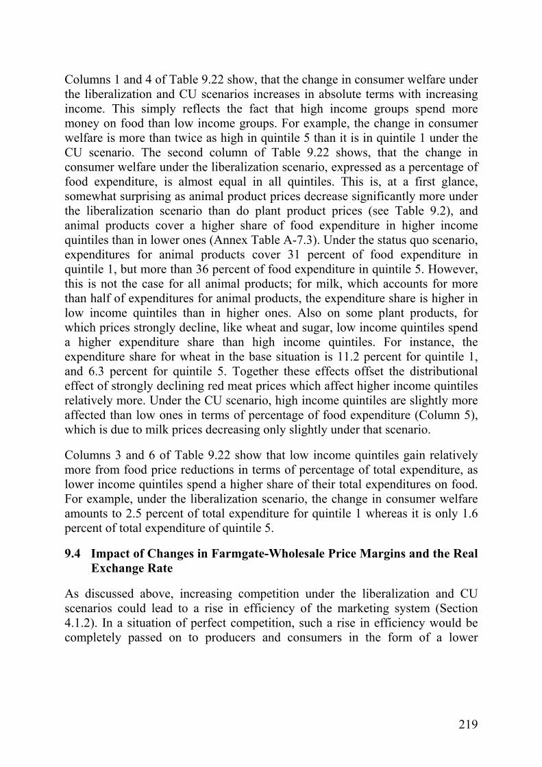
219

Columns 1 and 4 of Table 9.22 show, that the change in consumer welfare under the liberalization and CU scenarios increases in absolute terms with increasing income. This simply reflects the fact that high income groups spend more money on food than low income groups. For example, the change in consumer welfare is more than twice as high in quintile 5 than it is in quintile 1 under the CU scenario. The second column of Table 9.22 shows, that the change in consumer welfare under the liberalization scenario, expressed as a percentage of food expenditure, is almost equal in all quintiles. This is, at a first glance, somewhat surprising as animal product prices decrease significantly more under the liberalization scenario than do plant product prices (see Table 9.2), and animal products cover a higher share of food expenditure in higher income quintiles than in lower ones (Annex Table A-7.3). Under the status quo scenario, expenditures for animal products cover 31 percent of food expenditure in quintile 1, but more than 36 percent of food expenditure in quintile 5. However, this is not the case for all animal products; for milk, which accounts for more than half of expenditures for animal products, the expenditure share is higher in low income quintiles than in higher ones. Also on some plant products, for which prices strongly decline, like wheat and sugar, low income quintiles spend a higher expenditure share than high income quintiles. For instance, the expenditure share for wheat in the base situation is 11.2 percent for quintile 1, and 6.3 percent for quintile 5. Together these effects offset the distributional effect of strongly declining red meat prices which affect higher income quintiles relatively more. Under the CU scenario, high income quintiles are slightly more affected than low ones in terms of percentage of food expenditure (Column 5), which is due to milk prices decreasing only slightly under that scenario.

Columns 3 and 6 of Table 9.22 show that low income quintiles gain relatively more from food price reductions in terms of percentage of total expenditure, as lower income quintiles spend a higher share of their total expenditures on food. For example, under the liberalization scenario, the change in consumer welfare amounts to 2.5 percent of total expenditure for quintile 1 whereas it is only 1.6 percent of total expenditure of quintile 5.

9.4 Impact of Changes in Farmgate-Wholesale Price Margins and the Real Exchange Rate

As discussed above, increasing competition under the liberalization and CU scenarios could lead to a rise in efficiency of the marketing system (Section 4.1.2). In a situation of perfect competition, such a rise in efficiency would be completely passed on to producers and consumers in the form of a lower

220

marketing margin.64 The results of such a decrease in margins are presented in Table 9.23.

Table 9.23: Effects of Decreasing Farmgate-Wholesale Price Margins (mill. €)

Liberalization scenario CU scenario

Margin –10% Margin + waste –10%

Margin –10% Margin + waste –10%

Absolute change

Relative change

Absolute change

Relative change

Abs. change

Relative change

Abs. change

Relative change

Change in agr. net imports

273 -15.0% 607 -33.7% 274 -54.5% 603 -119.9%

Change in prod. surplus

488 -18.1% 693 -25.7% 506 -49.2% 687 -66.9%

Change in cons. welfare

26 0.7% 52 1.5% 72 4.7% 132 8.7%

Change in total welfare

514 75.5% 745 109.6% 577 110.7% 819 157.2%

Source: Own calculations.

Table 9.23 shows that a relatively small reduction of the relative and the absolute components of the processing margin (see Section 5.3) by 10 percent has a significant impact on trade and welfare. Under the liberalization scenario, a decrease of 10 percent of the processing margin leads to a reduction of net imports by €273 million, or 15 percent of total net imports. The positive effect of decreasing margins on producer surplus is €488 million and the change in consumer welfare of decreasing margins is €26 million. Overall welfare effects are €514 million, which is 77 percent of the welfare effects of the liberalization scenario, without any change in margins. If also the share of waste, which contributes to the total margin between farmgate and wholesale price (see above Section 5.3), is reduced by 10 percent, trade and welfare effects are even higher; total welfare increases by €745 million under the liberalization scenario.

64 A decrease of the marketing margin coupled with real improvements in technical efficiency, could also result from firms in the marketing chain being forced to pass on part of their producer rent to consumers and farmers. This effect would have mainly distributional rather than allocational effects and is not analyzed in this study.

221

Turkey is a country with a highly volatile exchange rate and strong inflation. Between the TURKSIM base period and January 2003 the nominal exchange rate of the Turkish Lira against the Euro increased by more than 1000 percent. Under the TURKSIM scenarios presented above, the assumption is that the real exchange rate remains constant over the projection period. This, however, is somewhat questionable as the Turkish Lira declined against the Euro by 6.6 percent in real terms between the TURKSIM base period and January 2003.65 Therefore TURKSIM is again solved under the assumptions of the real exchange rate increasing by 10 percent and the real exchange rate decreasing by 10 percent over the projection period. Table 9.24 shows results of these calculations. Agricultural prices increase with a real devaluation of the Turkish Lira by 6.1 to 8.9 percent under the different scenarios. The increase of production value is somewhat higher due to increased production quantities. In contrast, with a constant real exchange rate, Turkey is a net exporter of agricultural products under all scenarios. In the case of real appreciation of the Turkish Lira, domestic prices and agricultural production value decrease and Turkey is a net importer of agricultural products under all scenarios.

Welfare effects under both the liberalization and the CU scenarios are somewhat lower in the case of devaluation, and somewhat higher with an appreciation of the Turkish Lira than they are with a constant real exchange rate. This is because prices fall more significantly as a result of liberalization or a CU with appreciation scenario; protection under the status quo scenario is higher. Aggregate welfare results, however, are in the same order of magnitude under differing assumptions with respect to the real exchange rate.

65 The real exchange rate is calculated as the nominal exchange rate multiplied by the EU Harmonised Consumer Price Index (as provided by the EUROPEAN CENTRAL BANK), divided by the Turkish Consumer Price Index (as provided by SIS).

222

Table 9.24: Effects of Real Devaluation and Appreciation of the Turkish Lira

Average farmgate

price

Pro-duction value

Net trade

Change in prod. surplus

Change in cons.

welfare

Change in total welfare

(€/t, quantity weighted)

(mill. €) (mill. €) (mill. €) (mill. €) (mill. €)

Standard Status quo 315 28,328 332 Liberalization 278 24,027 -1,816 -2,745 3,470 667CU 301 26,796 -503 -1,063 1,523 482

Devaluation 10 percent

Status quo 335 31,051 1,961 Absolute change 19 2,724 1,630 Relative change 6.1% 9.6% 491.3%

Liberalization 303 27,298 243 -2,430 3,006 525Absolute change 25 3,271 2,059 315 -464 -141Relative change 8.9% 13.6% -113.4% -11.5% -13.4% -21.1%

CU 323 29,954 1,431 -854 1,245 410Absolute change 23 3,158 1,935 209 -278 -72Relative change 7.5% 11.8% -384.4% -19.6% -18.3% -14.9%

Appreciation 10 percent

Status quo 304 26,745 -619 Absolute change -12 -1,582 -951 Relative change -3.7% -5.6% -286.7%

Liberalization 260 21,905 -3,197 -3,067 3,974 908Absolute change -18 -2,123 -1,382 -322 504 241Relative change -6.5% -8.8% 76.1% 11.7% 14.5% 36.1%

CU 281 24,360 -1,998 -1,509 2,059 560Absolute change -19 -2,435 -1,494 -446 536 78Relative change -6.4% -9.1% 296.9% 42.0% 35.2% 16.1%

Source: Own calculations.

223

10 CONCLUSIONS

Turkey has liberalized its agricultural markets significantly in recent years. For future policy design, several options exist, three of which are analyzed in the framework of this study. First, the maintenance of the degree of market intervention at the level of 1996/98 is analyzed. This option is somewhat outdated by actual policy developments as Turkey has, under the World Bank-supported agricultural policy reform program, lowered protection levels for some products, and intends to continue on this path. Second and third, scenarios of complete agricultural trade liberalization or unilateral agricultural trade liberalization in the CU with the EU are analyzed. It appears that the option of an inclusion of agriculture in the CU with the EU is very similar to the option of complete liberalization of agricultural trade for most products. This is because the EU has, in recent years, significantly liberalized its agricultural markets and is projected to continue to do so for many reasons, including the WTO process, Eastern enlargement, and an interest in further liberalizing trade in the framework of bilateral agreements.

At first, the principal question of whether or not to liberalize the Turkish agricultural sector is discussed because such a liberalization would also be part of the CU option for most products, too. Then, the question as to whether the agricultural sector should be liberalized completely or whether it should be liberalized within a CU with the EU is addressed.

10.1 Liberalization of the Agricultural Sector

The complete liberalization of the agricultural sector leads to significant static comparative welfare gains as shown above. For the year 2006, these welfare gains are estimated at about €670 million or about 2.3 percent of projected agricultural production value, or 0.4 percent of projected GDP. If one adds the assumption that, due to increased competition, marketing margins decrease by 10 percent, welfare gains could even be about €1,400 million. These results have shown to be relatively stable even in the face of variation of critical exogenous parameters like the real exchange rate, the shadow price for sugar, and supply and demand shifters. Other dynamic gains, like enhanced productivity growth rates, are not covered by simulations in the framework of this study.

However, aside from aggregated welfare gains, distributional aspects are important. At the consumption side, the liberalization of the agricultural sector leads to a more equal distribution of real income in relative terms because lower income groups spend a higher share of their income on food and therefore gain relatively more from lower food prices. At the production side, the liberalization of the agricultural sector reduces intrasectoral income inequality in absolute

224

terms, as large and wealthy farms receive most of the gains in producer surplus resulting from current price support due to their high share in production.

One other major distributional effect of liberalization of agricultural policies, however, may conflict with the interests of Turkish policy makers: the distribution from producers to consumers and thus from rural to urban areas. The 1994 income survey shows the mean income in rural areas as 24 percent lower than in urban areas (SIS, 1997). In 1994 the poverty gap in rural areas, indicating the share of total income that has to be transferred to the poor in order to raise all poor to the poverty line, was about 30 percent higher than in urban areas, with the poverty line set at half the median income (Cakmak, 1998).

TURKSIM results overestimate the effect of shifting income from producers to consumers because agricultural producers also act as consumers and do therefore capture part of the loss of producer surplus in the form of the compensating variation at the consumption side. Nonetheless, land owners and agricultural producers of most products clearly lose from liberalization in the comparative static framework of TURKSIM. Even if one reduces total losses of €2,749 million by one-third due to the share of agricultural producers in total food consumption, the resulting losses of about €1,833 million still account for about 6.4 percent of projected production value in 2006. As about 90 percent of agricultural producers in Turkey operate exclusively on their own land (SIS, 1994), and tenancy of land is of low significance in Turkey, most of these losses must be borne by farmers and would not be passed on to land owners due to lower land leasing prices.

Various options for poverty reduction measures and measures to support rural areas exist as alternatives to shifting money from taxpayers and consumers mainly to large producers by price supporting policies. Policies aiming better at social and regional development objectives include enhanced public investment in rural infrastructure such as schools, roads, medical care, and so on. People in rural areas benefit from such policies more equally, independent of their farm size or income source. Furthermore productivity in agriculture has the potential to increase significantly through investments in education of farmers, as almost no training opportunities for farmers exist in the current situation. Finally, for the purpose of poverty reduction, direct payments to small farmers are an alternative which is currently implemented under the agricultural policy reform package. Major drawbacks of such payments are the administrative and budgetary requirements. The budget revenue required to finance direct payments could be generated by imposing a low tax on food consumers in order to avoid the possibly negative distributional effects of additional income taxation (see below). If transaction costs of direct payments are not too high, consumers would still be better off with the introduction of such a tax under liberalization

225

because the gross price of food would fall by more than the tax required to finance income transfers to needy groups of producers.

One last distributional effect of liberalizing agricultural markets in Turkey should at least be mentioned. Subsidizing agriculture withdraws resources from other parts of the economy directly by shifting taxpayers’ money, and indirectly via the impact on factor markets and the real exchange rate. Therefore, liberalizing the agricultural sector will have positive effects on other sectors of the economy. These general equilibrium effects could indeed generate positive welfare effects significantly larger than those resulting from the partial equilibrium model used in this study.

In terms of policy priorities it seems reasonable for Turkey to first do away with all remains of budget-financed agricultural market policies, such as intervention buying, export subsidies, input subsidies, and producer premiums. This is because, in addition to the negative comparative static negative welfare effects of such measures, budget-financed support is subject to transaction costs in the context of collecting and distributing taxpayers money. Some of these transaction costs are unavoidable, but for Turkey these transaction costs are especially problematic:

"...the tax system in Turkey is believed to be very inefficient, limited in its coverage, full of leakages and critically depends on the income taxes from fixed income wage and salary earners and indirect taxes collected from consumers. Different estimates show that the size of the untaxed/unrecorded economy in Turkey reaches 30 to 50 per cent of total GNP. It is therefore not too unrealistic to expect that the transfers to agriculture from taxpayers have a relatively larger burden on middle and lower income groups than on higher income groups..." (Cakmak, 1998, p. 9).

In such a situation the collection of taxes itself probably has a negative effect on income distribution and it is of special importance to limit budgetary outlays to efficient policies well aimed at socially accepted goals.

The second step of liberalizing the agricultural sector after abolition of budget-financed market policies would be the reduction of tariffs. Several considerations play a role when thinking about the timing of tariff abolition. Cereals are protected strongly in the current situation. To reduce cereal tariffs at an early stage of the reform process would have two advantages. First, cereals cover a high share of consumption expenditures in low income groups. Price reductions would, therefore, especially relieve the situation of poor consumer groups. Secondly, reductions of cereal prices would increase competitiveness of

226

animal production. An early commitment not to rise domestic price levels for cereals significantly above the international price level could therefore increase the willingness of producers to invest especially in the relatively competitive poultry and egg sectors. Tariff reductions for animal products should be carried out according to a long-term, transparent schedule as animal production often requires long-term investments of farmers and sudden price movements can endanger the ability of farmers to pay off these investments.

Furthermore from an economic point of view, it would make sense to decrease tariffs first for products which are more highly subsidized in order to reduce intrasectoral distortions of the production program. In the area of plant products, this is especially the case for sugar. Welfare effects of a reduced sugar price could be considerable, dependent on the current shadow price for sugar; competitiveness of other products for which Turkey has a comparative advantage in production would increase. Another product for which there is an enormous peak in protection is tea. In that case, however, production is geographically concentrated and limited to the Black Sea region, and producers are highly specialized and generally small-scale farmers. Options for the diversification of agricultural production should therefore be investigated and for a limited period of time tariff protection may be the best solution for the Turkish government to transfer money to tea producers as an alternative to direct payments which have to be financed from the budget.

10.2 Extension of the CU with the EU to Cover Agricultural Products

As discussed above, the degree of liberalization does not differ much between the liberalization and the CU scenarios for most products. The most important price differences are higher prices for sugar, milk, and sheep meat under the CU scenario. The total welfare gain under the customs union scenario is about €200 million lower than under the liberalization scenario. This is mainly due to lower welfare gains for milk, and somewhat less to sheep meat. The welfare difference for sugar is relatively low as the price reduction under the liberalization scenario has little effect on allocation because of the shadow price being significantly below the market price under the status quo scenario, together with a low price elasticity of demand for sugar. Dependent on the assumptions made on the shadow price for sugar in the base situation, the difference in welfare gains for sugar under the liberalization and the CU scenarios could be more significant.

Compared to the status quo and the liberalization scenario, the CU scenario would be equivalent to a "partial liberalization" of the Turkish milk and sheep meat market as prices would be lower than under the status quo scenario, with the resulting "partial welfare gains." Still EU reform of agricultural markets will

227

proceed, and for milk and sugar, options for further price reductions are currently under discussion.

The pure terms of trade effect of a CU as defined above is surprisingly small. Turkey would gain about €60 million of export revenue because of export prices above world market level for some fruits and vegetables, and would lose about €50 million because of import prices above world market level for milk products. This result, however, is conditional on several assumptions made. First, it depends on the assumptions made about shifters of supply and demand (see Table 9.17). If supply shifters turn out to be higher, or demand shifters turn out to be lower than assumed here, the terms of trade effects would be higher for exported fruits and vegetables and lower for the import product milk.

Secondly, an important assumption made above influencing the terms of trade effect is that the abolition of the entry price system for fruits and vegetables would have no significant impact on Turkish prices due to high transportation cost and highly priced Turkish supply of high quality products (Section 2.2.3). But Turkey's currently disadvantageous geographic location for exports of fresh products to the EU could considerably improve if Central European countries join the EU from 2004 on, and their import demand increases due to increasing income. Central European markets may also be more suitable for somewhat lower qualities at lower prices than north European markets.

Finally it is maintained that the degree of policy harmonization between Turkey and the EU, as potentially "... required to establish freedom of movement of agricultural products" (Art. 23:1, Customs Union Decision) is, from a purely economic point of view, very limited. As discussed above (Section 4.3.2) all kinds of direct payments, input subsidies, and rural development measures could remain under purely national/EU responsibility. Sugar is projected to be the only product for which Turkey would probably need to apply a supply control system not to exceed 100 percent self-sufficiency.

A problem might arise from the fact that tariff revenue for third country (i.e. non-EU) imports coming into Turkey would still accrue to the Turkish budget. This would be a strong incentive for the Turkish government to promote imports from third countries (rather than from the EU) for those products where the EU price is much above world market level (for example dairy products). This could even lead to a situation where Turkey, being a net importer of the product concerned, would export some of its domestic production to the EU while importing the same product from third countries at a lower price. The most straightforward way to deal with this problem would be to have a common budget with the EU for tariff revenue. An alternative, possibly easier to implement, would be that Turkey's tariff revenue for agricultural products would

228

directly accrue to the EU budget. The EU, on the other hand, could compensate Turkey by a lump sum to be paid each year which would be independent from actual tariff revenue. The incentive for Turkey to import products from third countries for which the EU is a net exporter would thus be removed.

Based on simulations made in this study, it seems that comparative static welfare effects do not clearly favor or disfavor an inclusion of agriculture in the CU with the EU, compared to a unilateral liberalization. The relevance of higher export prices and lower import prices for some products is estimated to be small, if determining factors are varied (see Table 9.17). The main difference is that liberalization would be slower for some products in the CU (sheep, sugar, milk) than it could be in the event of reduction of Turkish MFN trade policies.

There are other reasons that could be relevant for Turkey when determining the intensity of its efforts for further liberalization of agricultural trade with the EU. If Turkish policy makers intend to liberalize agricultural markets due to motives of efficiency, budgetary austerity, and income distribution, it may be easier to do so in a CU than on a MFN basis. This is because liberalization may be easier to defend to the Turkish public if it "must be done" because of the CU. The CU could therefore have the same self-binding function for Turkish policymakers as the WTO process has had for many politicians in industrialized countries.

The stabilization of agricultural trade policies because of their long-term binding in a CU could also have positive effects on the disposition for domestic and foreign investments in the Turkish food processing industry. Also, the further harmonization of product and processing standards, which would probably go along with a CU, may enhance this disposition and could result in gains from trade for Turkey as well as for the EU.

It may also be of importance to know how Turkey's position in the negotiating process with the EU on further integration would be influenced by its position with respect to the integration of agricultural markets. In other words, if the EU is interested in agricultural integration, would Turkey's negotiating capital increase with a readiness to remove agricultural trade barriers? Or would Turkey have to pay a political price for the further integration of agricultural markets?

Finally, as Turkish membership draws closer, the integration of agricultural markets would include the possibility of a smooth transition period instead of a sudden adjustment in the event of full membership. This argument, however, is considered premature as full EU membership of Turkey will probably not take place before 2010, and the CAP is a rapidly moving target. Turkey should therefore base its policy on the expected short- to mid-term advantages and disadvantages of a CU in agriculture.

229

REFERENCES

AgraEurope (London) Ltd. (2003), CAP Monitor. Akder, H. et al. (1990), Turkish Agriculture and European Community Policies,

Issues, Strategies and Institutional Adaptation. Report of a study for the United Nations Development Programme, executed by the United Nations Conference on Trade and Development.

Aksoy, I. (2000), Programi Iki Projeyle Devam Ediyor Süt ve Süt ürünleri. Dunya (ekonomi-politika) Gazetesi. 21 August.

Altundag, S. and T. Günes (1992), Tükyie' de Patatesve Soganin Üretim Miktari Ile Fiyat Iliskileri. Published by Ankara University.

Anderson, K. and R. Tyers (1993), Implication of EU Expansion for European Agricultural Policies, Trade and Welfare. CEPR Discussion Paper No. 829, Centre for Economic Policy Research.

Balkhausen, O. (2003), Agrarpolitische Maßnahmen zur Erhaltung nationaler Tier- und Verbraucherschutzstandards im Zuge fortschreitender Handelsliberalisierung. Masterarbeit im wissenschaftlichen Studiengang Agrarwissenschaften an der Georg-August-Universität Göttingen, Fakultät für Agrarwissenschaften, Institut für Agrarökonomie.

Bayaner, A. (1996), Supply Response for Major Crops in Turkey. University of Reading.

Bayaner, A., and D. Hallam (1996), The Effects of Macroeconomic Changes on Turkish Agriculture. Discussion Paper 4/96, University of Reading, UK.

Beghin, J. (1997), Final Report. FAO Final Report of Project TCP/TUR/4552, Assistance for Agricultural Policy Reform in Turkey in Relation to EU and WTO Agreements, 2 May.

Behrman, J. R. and A. B. Deolalikar (1987), Will Developing Country Nutrition Improve with Income? A Case Study for Rural South India. Journal of Political Economy. Vol. 95, pp. 492-507.

Behrman, J. R. and B. L. Wolfe (1984), More Evidence on Nutrition Demand, Income Seems Overrated and Women's Schooling Underemphasized. Journal of Development Economics. Vol. 14, pp. 105-28.

Bouis, H. E. (1994), The Effect of Income on Demand for Food in Poor Countries: Are our Food Consumption Databases Giving us Reliable Estimates? Journal of Development Economics. Vol. 44, pp. 199-226.

Brosig, S. (2000), Die Private Nachfrage nach Nahrungsmitteln im Transformationsprozess Tschechiens und Polens.

230

Cakmak, E. (1998), Agricultural Policy Reforms and Rural Development in Turkey. Economic Development and Poverty Reduction Workshop. Mediterranean Development Forum, September 3-6, Marrakech, Morocco. Online version at http://www.worldbank.org/mdf/mdf2/papers/econdev/cakmak.pdf

Cakmak, E and H. Kasnakoglu (2001), Tarim Sektöründe Türkiye ve Avrupa Birligi Etkilesimi: Türkiye 'nin AB'ye Üyeliginin Analizi. Proje Raporu 2001-18. Agricultural Economics Research Institute. Ankara, August.

Cox, T. L. and M. K. Wohlgenant (1986), Prices and Quality Effects in Cross-Sectional Demand Analysis. American Journal of Agricultural Economics. Vol. 68, pp. 908-19.

Cramer, J. S. (1973), Interaction of Income and Price in Consumer Demand. International Economic Review. Vol. 14, pp. 351-63.

Deaton, A. and J. Muellbauer (1980), Economics and Consumer Behaviour. European Commission (1999), Agricultural Prices, Price Indices and Absolute

Prices, Data 1989-1998. European Commission (2003), Explanatory Memorandum and Legislative

Proposals for CAP Reform. COM(2003) 23 final, 21. January. Online version at http://europa.eu.int/comm/agriculture/mtr/memo_en.pdf

European Commission (various issues), Agricultural Markets, Prices. European Commission (various issues), The Agricultural Situation in the

European Union. European Communities (2002), Agricultural Prices – Price Indices and

Absolute Prices. Electronic version. Eurostat (various issues), Intra- and Extra-EU Trade. Electronic version. FAO (2002a), FAOSTAT database. http://apps.fao.org/cgi-bin/nph-

db.pl?subset=agriculture

FAO (2002b), FAO commodity balances 1996-2000. Electronic version, unpublished.

FAPRI (2002), Agricultural Outlook 2002. Feger, F. (2000), A Behavioral Model of the German Compound Feed Industry –

Functional Form, Flexibility and Regularity. Published at http://webdoc.sub.gwdg.de/diss/2000/feger/

Förster, M. F. (2000), Trends and Driving Factors in Income Distribution and Poverty in the OECD Area. Labor Market and Social Policy-Occasional Papers No. 42. OECD Document DEELSA/ELSA/WD(2000)3.

231

Frohberg, K. and G. Weber (2002), Auswirkung der EU-Osterweiterung im Agrarbereich. Discussion Paper Nr. 42, Institute of Agricultural Development in Central and Eastern Europe.

Fuller, F., A. A. Koc, H. Sengül and A. Bayaner (1999), Farm-Level Feed Demand in Turkey. Working Paper 99-WP 226, Center for Agricultural and Rural Development, Iowa State University.

GATT (1993), Modalities for the Establishment of Specific Binding Commitments under the Reform Programme: Note by the Chairman of the Market Access Group Document MTN.GNG/MA/W/24. Geneva, December 20.

GATT (1994), Schedules of Market Access Concessions. Electronic version, Geneva.

Gehrels, F. (1956-57), Customs Union from a Single-Country Viewpoint. In: Review of Economic Studies, 24 (1), pp. 61-4. Also published in Kowalczyk, C. (ed.) (1999), Economic Integration and International Trade. The International Library of Critical Writings in Economics 115, pp. 72-5.

Grethe, H. (1999), The potential extension of the Customs Union between Turkey and the EU – A report on the impact of including agricultural products in the Customs Union on the Turkish agricultural sector. In: FAO Agricultural Policy and Economic Development Series. No. 5.

Grethe, H. (2002a), Optionen für die Verlagerung von Haushaltsmitteln aus der ersten in die zweite Säule der EU-Agrarpolitik. In: Ländlicher Raum. No. 5 (53), pp. 9-15. Also published as Diskussionsbeitrag 0201, Institute of Agricultural Economics, Göttingen.

Grethe, H. (2002b), Potentielle Auswirkungen der ökologischen Agrarwende in der EU auf die Entwicklungsländer. Kurzstudie für das BMZ. DIE, Bonn.

Grethe, H. and A. Uzmay (2000), Entwicklung und gegenwärtiger Stand der Agrarprotektion in der Türkei und der EU am Beispiel ausgewählter Produkte. In: Verband deutsch-türkischer Agrar- und Naturwissenschaftler e. V. (Ed.), Deutsch-Türkische Agrarforschung – 6. Symposium, 27. September – 2. Oktober 1999, Justus-Liebig Universität Gießen.

Grethe, H. and S. Tangermann (1999a), The EU Import Regime for Fresh Fruit and Vegetables after Implementation of the Results of the Uruguay Round. Diskussionsbeitrag 9901 des Instituts für Agrarökonomie, Universität Göttingen.

Grethe, H. and S. Tangermann (1999b), The New Euro-Mediterranean Agreements, An Analysis of Trade Preferences. Diskussionsbeitrag 9902 des Instituts für Agrarökonomie, Universität Göttingen.

232

Grings, M. (1985), Ein Angebotsmodell für den Agrarsektor der Bundesrepublik Deutschland: Ökonometrische Schätzung auf der Grundlage der Dualitätstheorie. Schriften zur angewandten Ökonometrie, Heft 15.

Harrison, G. W., T. F. Rutherford and D. G. Tarr (1996), Economic Implications for Turkey of a Customs Union with the European Union. Policy Research Working Paper No. 1599, World Bank, International Economics Department, International Trade Division.

Heckelei, T. (2002), Calibration and Estimation of Programming Models for Agricultural Supply Analysis. Habilitationsschrift, Landwirtschaftliche Fakultät Bonn.

Hicks, W. W. and S. R. Johnson (1968), Quantity and Quality Components for Income Elasticities of Demand for Food. American Journal of Agricultural Economics. Vol. 50, pp. 1512-17.

Howitt, R. E. (1995), Positive Mathematical Programming. American Journal of Agricultural Economics. Vol. 77, pp. 329-42.

International Monetary Fund (2001), International Financial Statistics Yearbook 2001.

IOOC (2002), Production, Consumption and Trade Figures at http://www.internationaloliveoil.org/eng/EconomicalArea.html

Just, R. E., D. L. Hueth and A. Schmitz (1982), Applied Welfare Economics and Public Policy.

Kasnakoglu, H. and Cakmak, E. H. (1995), The Impact of the Uruguay Round on Agricultural Policies in Turkey.

Kasnakoglu, H. and A. A. Gurkan (1986), Output, Demand and Foreign Exchange Effects of Agricultural Price Policies in Turkey. Mimeo document for the World Bank project on Political Economy of Agricultural Price Policies.

Kirchgessner, M. (1992), Tierernährung. Koc, Ali A., B. D. B. Smith, F. Fuller and J. Fabiosa (1998), The Turkish

Agricultural Policy Analysis Model. Technical Report 98-TR 42. Center for Agricultural and Rural Development.

Kowalczyk, C. (1999), Introduction. In: Kowalczyk, C. (ed) Economic Integration and International Trade. The International Library of Critical Writings in Economics 115.

Layard, P. R. G. and A. A. Walters (1978), Microeconomic Theory. Lipsey, R. G. (1968), Economic Unions. In Sills, D. L. (ed.), International

Encyclopedia of the Social Sciences, pp. 541-7, New York.

233

McClatchy, D. (1997), Agricultural Policy Reform in Turkey Relating to WTO and EU Agreements – Findings and Conclusions. Report prepared for the FAO project "Assistance for Agricultural Policy Reform in Turkey in Relation to EU and WTO Agreements". November.

Manegold, D. (1988), Agrarpolitische Probleme einer Mitgliedschaft der Türkei in der Europäischen Gemeinschaft. Arbeitsbericht des Instituts für landwirtschaftliche Marktforschung der Bundesforschungsanstalt für Landwirtschaft Braunschweig-Völkenrode (FAL).

Meinheit, E. (1995), Handelspolitik als Umweltpolitik im Agrarbereich? Mercenier, J. and E. Yeldan (1996), On Turkey's Trade Policy: Is a Customs

Union With Europe Enough? Discussion Paper 96-4, Department of Economics, Bilkent University.

Münch, W. (2002), Effects of EU Enlargement to the Central European Countries on Agricultural Markets. CEGE-Schriften Band 4, Center for Globalization and Europeanization of the Economy, Georg-August-Universität Göttingen.

OECD (1987), National Policies and Agricultural Trade. OECD (1989), Impacts of Agricultural Reform on Production Inputs. Working

Party on Agricultural Policies and Markets of the Committee for Agriculture. Joint Working Party of the Committee for Agriculture and the Trade Committee.

OECD (1992), AGLINK: Introduction and Overview of the Main Characteristics. Working Party on Agricultural Policies and Markets of the Committee for Agriculture.

OECD (1998), Statwise PSE/CSE Database. OECD (2001a), PSE and CSE Database. Electronic version. OECD (2001b), Agricultural Policies in OECD Countries, Monitoring and

Evaluation 2001. OECD (2001c), OECD Economic Surveys, Turkey, February 2001. OECD (2001d), Agricultural Outlook 2001-2006. OECD (2002a), Agricultural Databases (electronic version). OECD (2002b), Agricultural Policies in OECD Countries, Monitoring and

Evaluation 2002. OECD (2002c), OECD Economic Outlook. No. 71. OJ, Official Journal of the European Communities (various issues).

234

Peeters, L. and Y. Surry (1994), Un modèle d'agrégation du secteur de l'alimentation animale au Benelux: une analyse préliminaire. Cahiers d'Economie et Sociologie Rurales. Vol. 30, pp. 50-70.

Peeters, L. and Y. Surry (1997), A Review of the Arts of Estimating Price-Responsiveness of Feed Demand in the European Union. Journal of Agricultural Economics. Vol. 48, pp. 379-92.

Phlips, L. (1983), Applied Consumption Analysis. Prais, S. J. and H. S. Houthakker (1955), The Analysis of Family Budgets. Robinson, S. and K. Thierfelder (1998), Trade Liberalization and Regional

Integration: The Search for Large Numbers. Paper presented to the meetings of the International Agricultural Trade Research Consortium (IATRC), Florida, December.

Roningen, V. O., J. Sullivan and P. M. Dixit (1991), Documentation of the Static World Policy Simulation (SWOPSIM) Modeling Framework. Staff Report AGES 9151, Economic Research Service, USDA.

Sadoulet, E. und Alain de Janvry (1995), Quantitative Development Policy Analysis.

Siebert, H. (1982), Zollunionen und Präferenzzonen. In: Handwörterbuch der Wirtschaftswissenschaften, pp. 666-78.

Southeastern Anatolia Project Regional Development Administration (1992), Agricultural Commodities Marketing Survey, Planning of Crop Pattern and Integration of Marketing and Crop Pattern Studies.

SIS (various issues), Agricultural Structure (Production, Price Value). SIS (various issues), External Trade Statistics (electronic version). SIS (various issues), Statistical Yearbook of Turkey. SIS (various issues), Wholesale Price Statistics. SIS (1990), 1987 Household Income and Consumption Expenditures Survey

Results. SIS (1994), General Agricultural Census, Results of the Agricultural Holdings

(Households) Survey. SIS (1997), 1994 Household Income and Consumption Expenditures Survey

Results. State Planning Organization (1990), The Southeastern Anatolia Project Master

Plan Study. State Planning Organization (1995), Seventh Five Year Development Plan

(1996-2000).

235

State Planning Organization (2001), Long-Term Strategy and Eight Five-Year Development Plan 2001-2005. Online version at http://ekutup.dpt.gov.tr/plan/viii/plan8i.pdf

Surry, Y. (1990), Econometric Modelling of the Compound Feed Sector. Journal of Agricultural Economics. Vol. 41, pp. 404-21.

Surry, Y. (1993), The "Constant Difference of Elasticities" Function with Applications to the EC Animal Feed Sector. Journal of Agricultural Economics. Vol. 44, pp. 110-25.

Tangermann, S. (1995), Implementation of the Uruguay Round Agreement on Agriculture by Major Developed Countries. Report prepared for UNCTAD. Document UNCTAD/ITD/16. Geneva, 3 October 1995.

Tangermann, S. (2000), Widening the EU to Central and Eastern European Countries: WTO and the Perspectives of the New Member States. In: Burrell, A, and A. Oskam (eds.), Agricultural Policy and Enlargement of the European Union, pp. 233-246.

Taylor, L. (1979), Macro Models for Developing Countries. Theil, H. (1952), Qualities, Prices and Budget Enquiries. The Review of

Economic Studies. Vol. 19, pp. 129-47. Tomato News (1994), Tomato News, 10/1994. Tomato News (2002), online production data at http://www.tomato-

news.com/tableau.htm

Twesten, H. (1999), Regional Trade Agreement in the GATT: An Assessment of the Legal Provisions. Supporting material for the "Training Session on WTO Issues in Preparation for the Next Round of Multilateral Trade Negotiations" organised by FAO, Prague, October 4-8.

Undersecretariat of Foreign Trade (various issues), Tariff Schedules (electronic version).

USDA (various issues), USDA GAIN Reports. http://www.fas.usda.gov/scriptsw/attacherep/default.asp

USDA (2002), SWOPSIM database. Electronic version at http://usda.mannlib.cornell.edu/data-sets/trade/92011/

Viner, J. (1950), The Customs Unions Issue. New York. Weise, C., M. Banse, W. Bode, B. Lippert, F. Nölle and S. Tangermann (2002),

Die Finanzierung der Osterweiterung der EU. Wahl, O., G. Weber and K. Frohberg (2000), Documentation of the Central and

Eastern European Countries Agricultural Simulation Model. Discussion

236

Paper No. 27, Institute of Agricultural Development in Central and Eastern Europe.

World Bank (2002), WDI online database. http://publications.worldbank.org/ecommerce/catalog/product?item_id=631625

World Bank (various issues), Global Commodity Markets. WTO (1996), Accession to the World Trade Organization, Information to be

Provided on Domestic Support and Export Subsidies in Agriculture. Technical Note by the Secretariat, Document WT/ACC/4, 18 March 1996.

WTO (2003), Negotiations on Agriculture, First Draft of Modalities for the Further Commitments. Document TN/AG/W/1, 17. February 2003.

WTO (various issues), Turkish WTO Notifications. Electronic versions at http://docsonline.wto.org/gen_search.asp

Annex

Ann

ex to

Cha

pter

3: O

verv

iew

of E

xist

ing

Pref

eren

ces G

rant

ed b

y th

e E

U fo

r Agr

icul

tura

l Im

port

s Ori

gina

ting

in

Turk

ey (a

s of A

pril

2001

),

CN

Cha

pter

1 -

Liv

e A

nim

als

No

MFN

bar

rier

M

FN b

arrie

r, no

pre

fere

nce

MFN

bar

rier,

parti

al p

refe

renc

e

MFN

bar

rier,

no b

arrie

r for

Tur

key

CN

cod

e Pr

oduc

t C

N c

ode

CN

cod

e Pr

oduc

t C

N c

ode

Prod

uct

0101

11

0101

1910

0102

10

0102

9090

0103

10

0103

9190

0103

9290

0104

1010

0106

0090

Pure

-bre

d br

eedi

ng h

orse

s H

orse

s for

slau

ghte

r Pu

re-b

red

bree

ding

bov

ines

Li

ve b

ovin

e an

imal

s Pu

re-b

red

bree

ding

swin

e Li

ve n

on-d

omes

tic sw

ine

" "

Pu

re-b

red

shee

p fo

r bre

edin

g

Oth

er li

ve a

nim

als

All

othe

r pr

oduc

ts

0102

9005

-79

Li

ve b

ovin

e an

imal

s01

0119

90

0101

20

0104

2010

01

0600

10

0106

0020

Hor

ses

Live

ass

es, m

ules

& h

inni

es

Pure

-bre

d br

eedi

ng g

oats

Li

ve d

omes

tic ra

bbits

Li

ve p

igeo

ns

Sour

ce: T

AR

IC, O

ffici

al J

ourn

al o

f the

Eur

opea

n C

omm

uniti

es, C

119

A, 2

3.04

.200

1.

239

Ann

ex to

Cha

pter

3, c

ontin

ued

CN

Cha

pter

2 -

Mea

t

No

MFN

bar

rier

M

FN

barr

ier,

no

pref

eren

ce

MFN

bar

rier,

parti

al p

refe

renc

e

MFN

bar

rier,

no b

arrie

r for

Tur

key

CN

cod

e Pr

oduc

t

CN

cod

e Pr

oduc

t C

N c

ode

Prod

uct

0203

1190

0203

1290

0203

1990

0203

2190

0203

2290

0203

2990

0206

1010

0206

1091

0206

1099

0206

21

0206

22

0206

2910

0206

2999

0206

3010

0206

4110

0206

49

0206

8010

0206

8099

0206

9010

0206

9099

0207

3410

0207

3490

0207

3681

0207

3685

0208

1090

0208

9020

0208

9040

Mea

t of s

win

e, n

ot

dom

estic

"

"

" "

"

"

" "

V

ario

us e

dibl

e of

fal

" "

"

"

" "

"

"

" "

"

"

" "

"

"

" "

"

"

" "

"

"

" "

M

eat a

nd o

ffal

of

poul

try

" "

"

"

Oth

er m

eat a

nd m

eat

offa

l "

"

All

othe

r pr

oduc

ts

0201

02

02

ex. 0

204

0206

1095

02

0629

91

0207

2510

02

0725

90

0207

2730

-70

02

1020

02

1090

41

0210

9090

Bov

ine

mea

t "

"

Goa

t & sh

eep

mea

t (a

bove

q. o

f 200

t)

Var

ious

edi

ble

offa

l "

"

With

in q

uota

of 1

,000

t:

Mea

t and

off

al o

f pou

ltry

" "

"

"

Bov

ine

mea

t "

"

Mea

t flo

ur

ex 0

204

0205

02

0680

9102

0690

9102

0713

9102

0714

9102

0726

9102

0727

9102

0735

9102

0810

1102

0810

1902

0820

0002

0890

5002

0890

6002

0890

80ex

021

0:

0210

1190

0210

1290

0210

1990

0210

9010

0210

9021

0210

9029

0210

9049

0210

9060

0210

9071

0210

9079

0210

9080

Goa

t & sh

eep

(with

in q

. of 2

00 t)

H

orse

mea

t V

ario

us e

dibl

e of

fal

" "

M

eat a

nd e

dibl

e of

fal o

f pou

ltry

" "

"

"

" "

"

"

Oth

er m

eat a

nd e

dibl

e m

eat o

ffal

"

"

" "

"

"

" "

"

"

Pres

erve

d:

Mea

t of s

win

e, n

ot d

omes

tic

" "

"

"

Hor

se m

eat

Mea

t of r

eind

eer

Oth

er...

O

ther

...

Shee

p an

d go

at m

eat

Pres

erve

d po

ultry

live

r "

"

Oth

er

240

Ann

ex to

Cha

pter

3, c

ontin

ued

CN

Cha

pter

4 -

Dai

ry P

rodu

cts,

Egg

s, H

oney

No

MFN

bar

rier

M

FN

barr

ier,

no

pref

eren

ce

MFN

bar

rier,

parti

al p

refe

renc

e

MFN

bar

rier,

no b

arrie

r for

Tur

key

CN

cod

e Pr

oduc

t

CN

cod

e Pr

oduc

t C

N c

ode

Prod

uct

0408

1120

0408

1920

0408

9120

0408

9920

Egg

yolk

s, no

t for

co

nsum

ptio

n "

"

Drie

d eg

gs, n

ot fo

r co

nsum

ptio

n Eg

gs, n

ot fo

r co

nsum

ptio

n

All

othe

r pr

oduc

ts

0403

1051

-99

0403

9071

-99

0405

2010

04

0520

30

Che

ese

abov

e qu

ota

(1,5

00 t)

: ex

040

6902

9 ex

040

6903

1 ex

040

6905

0 ex

040

6908

6 ex

040

6908

7 ex

040

6908

8

Flav

oure

d yo

gurt

But

term

ilk...

, fla

vour

edD

airy

spre

ads

"

"

Abo

ve q

uota

che

ese

" "

"

"

" "

"

"

" "

0406

2010

04

0690

19

0407

0090

04

09

0410

C

hees

e w

ithin

qu

ota

(1,5

00 t)

: ex

040

6902

9

ex 0

4069

031

ex 0

4069

050

ex

040

6908

6 ex

040

6908

7 ex

040

6908

8

Gre

ated

or p

owd.

che

ese

Oth

er c

hees

e Eg

gs (e

xcl.

poul

try e

ggs)

H

oney

Tu

rtles

' egg

s & o

ther

s W

ithin

quo

ta c

hees

e "

"

" "

"

"

" "

"

"

CN

Cha

pter

5 -

Prod

ucts

of A

nim

al O

rigi

n no

t Els

ewhe

re S

peci

fied

No

MFN

bar

rier

M

FN b

arrie

r, no

pre

fere

nce

MFN

bar

rier,

parti

al p

refe

renc

e

MFN

bar

rier,

no b

arrie

r for

Tur

key

CN

cod

e Pr

oduc

t

CN

cod

e Pr

oduc

t C

N c

ode

Prod

uct

All

othe

r pr

oduc

ts

0509

0090

N

atur

al sp

onge

s

241

Ann

ex to

Cha

pter

3, c

ontin

ued

CN

Cha

pter

6 -

Liv

e Pl

ants

and

Flo

wer

s

No

MFN

bar

rier

MFN

bar

rier,

no p

refe

renc

eM

FN b

arrie

r, pa

rtial

pre

fere

nce

MFN

bar

rier,

no b

arrie

r for

Tur

key

CN

cod

e Pr

oduc

t

CN

cod

e Pr

oduc

t C

N c

ode

Prod

uct

0601

2010

06

0210

10

0602

2010

06

0290

20

0604

1010

06

0499

10

Chi

cory

pla

nts a

nd ro

ots

Unr

oote

d vi

ne c

uttin

gs

Vin

e sl

ips

Pine

appl

e pl

ants

M

osse

s and

lich

ens

" "

A

ll ot

her

prod

ucts

242

Ann

ex to

Cha

pter

3, c

ontin

ued

CN

Cha

pter

7 -

Veg

etab

les

No

MFN

bar

rier

M

FN b

arrie

r, no

pre

fere

nce

M

FN b

arrie

r, pa

rtial

pre

fere

nce

M

FN

barr

ier,

no

barr

ier f

or

Turk

ey

CN

cod

e Pr

oduc

t C

N c

ode

Prod

uct

CN

cod

e Pr

oduc

t

0709

6091

07

0960

95

0712

9011

07

1310

-40

Cap

sicu

m

Cap

sicu

m

Cor

n (f

or

sow

ing)

D

ried

leg.

ve

geta

bles

spec

ific

tari

ffs:

0709

9039

07

0990

60

0711

2090

07

1190

30

0712

9019

07

1410

10

0714

1091

07

1410

99

0714

9011

-19

Ad v

alor

em ta

riffs

:ex

070

1905

0 ex

070

3101

1, -1

9 ex

070

820

ex 0

7089

0 ex

070

930

ex 0

7094

0 ex

070

9907

0 ex

070

9909

0 ex

070

9909

0

Oliv

es fo

r oil

prod

uctio

n Fr

esh

swee

tcor

n O

lives

, pro

visi

onal

ly p

rese

rved

Sw

eetc

orn,

pro

visi

onal

ly p

rese

rved

D

ried

swee

tcor

n Pe

llets

of m

anio

c flo

ur

Froz

en m

anio

c Fr

esh

man

ioc

Arr

owro

ot

Pota

toes

, 1.4

-31.

12

Oni

ons,1

6.5-

14.2

, abo

ve q

. of 2

,000

t B

eans

, 1.5

-31.

10

Bea

ns, 1

.5-3

0.6

Eggp

lant

, 1.5

-14.

01, a

bove

q. o

f 1,0

00 t

Cel

ery,

1.5

-31.

12

Cou

rget

tes,

1.3-

30.1

1, a

bove

q. o

f 500

tPu

mpk

in, 1

.3-3

0.11

W

ild o

nion

s, 16

.5-1

4.2

0702

07

07 (e

xcl.

0707

0090

) 07

0910

ex

070

930

ex 0

7093

0 ex

070

9907

0 ex

070

9907

0

Tom

atoe

s (EP

) C

ucum

bers

(EP)

A

rtich

okes

, 1.1

1-30

.6

(EP)

Eg

gpla

nt, 1

5.1-

30.4

(E

P)

Eggp

lant

, 1.5

-14.

1 in

qu

ota

of 1

,000

t (E

P)

Cou

rget

tes,

1.12

-28.

2 (E

P)

Cou

rget

tes,

1.3-

30.1

1 in

quo

ta o

f 500

t (E

P)

All

othe

r pr

oduc

ts

243

Ann

ex to

Cha

pter

3, c

ontin

ued

CN

Cha

pter

8 -

Frui

t and

Nut

s

No

MFN

bar

rier

M

FN b

arrie

r, no

pre

fere

nce

M

FN b

arrie

r, pa

rtial

pre

fere

nce

M

FN

barr

ier,

no

barr

ier f

or

Turk

ey

CN

cod

e Pr

oduc

t C

N c

ode

Prod

uct

CN

cod

e Pr

oduc

t

0801

08

0211

10

0802

1210

08

0290

20

0804

50

0807

20

0810

4010

08

1090

30-

40

0813

4060

-70

Coc

onut

s, ca

shew

B

itter

alm

onds

in

shel

l B

itter

alm

onds

A

reka

nut

s G

uava

s, m

ango

es

Papa

yas

Cow

berr

ies

Oth

er fr

uit

Drie

d ta

mar

inds

...

0803

0019

ex

080

6101

0ex

080

711

ex 0

8071

9 ex

080

9400

5

Ban

anas

G

rape

s, 1.

5-17

.6, 1

.8-1

4.11

W

ater

mel

ons,

16.6

-31.

3,

abov

e q.

of 1

4,00

0 t

Mel

ons,

1.6-

31.1

0,

Plum

s, 16

.6-3

0.4

0802

21-2

2 ex

080

510

(exc

l. 08

0510

80)

ex 0

8052

0

0805

3010

ex

080

6101

0 08

0810

20-9

0 ex

080

8205

0 ex

080

910

ex 0

8092

0 ex

080

930

ex 0

8094

005

ex 0

8111

011,

ex

081

1201

1,

ex 0

8119

019

0811

9011

Haz

elnu

ts

Ora

nges

(EP)

, 1.1

2-31

.5

Man

darin

s, 1.

11-2

8.2

(EP)

Le

mon

s (EP

) G

rape

s, 21

.7-3

1.7,

15.

11-

20.1

1 (E

P)

App

les (

EP)

Pear

s, 1.

7-30

.4 (E

P)

Apr

icot

s, 1.

6-31

.7 (E

P)

Che

rrie

s, 21

.5-1

0.8

(EP)

Pe

ache

s, 11

.6-3

0.09

(EP)

Pl

ums,

11.6

-15.

6 (E

P)

Froz

en st

raw

berr

ies,

abov

e qu

ota

of 1

00 t

"…"

"…"

Oth

er...

All

othe

r pr

oduc

ts

244

Ann

ex to

Cha

pter

3, c

ontin

ued

CN

Cha

pter

9 -

Cof

fee,

Tea

, Mat

e

No

MFN

bar

rier

M

FN b

arrie

r, no

pr

efer

ence

M

FN b

arrie

r, pa

rtial

pre

fere

nce

M

FN b

arrie

r, no

bar

rier f

or T

urke

y

CN

cod

e Pr

oduc

t

CN

cod

e Pr

oduc

t C

N c

ode

Prod

uct

0902

20

0902

30

0902

40

0903

09

0411

09

0420

30

0906

09

08

0909

09

1010

09

2010

09

1030

09

1040

11

0910

50

0910

9910

09

1091

10

0910

9991

Gre

en te

a, >

3 kg

B

lack

ferm

ente

d te

a, <

3 kg

B

lack

ferm

ente

d te

a, >

3 kg

M

ate

Pepp

er

Cap

sicu

m &

pim

enta

C

inna

mon

N

utm

eg, m

ace,

car

dam

oms

Ani

se a

nd o

ther

seed

s G

inge

r Sa

fran

Tu

rmer

ic c

urcu

ma

Wild

thym

e C

urry

Fe

nugr

eek

seed

O

ther

spic

es

Oth

er sp

ices

, nei

ther

cru

shed

no

r gro

und

A

ll ot

her p

rodu

cts

245

Ann

ex to

Cha

pter

3, c

ontin

ued

CN

Cha

pter

10

- Cer

eals

N

o M

FN b

arrie

r

MFN

bar

rier,

no p

refe

renc

e M

FN b

arrie

r, pa

rtial

pre

fere

nce

M

FN b

arrie

r, no

bar

rier f

or T

urke

y

CN

cod

e Pr

oduc

t

CN

cod

ePr

oduc

t C

N c

ode

Prod

uct

1005

1011

-19

1008

30

Hyb

rid m

aize

seed

C

anar

y se

ed

All

othe

r pr

oduc

ts

1001

10

1002

Dur

um w

heat

R

ye

1001

9010

10

0610

10

1007

0010

Spel

t for

sow

ing

Ric

e in

hus

k fo

r sow

ing

Hyb

rid so

rghu

m, f

or so

win

g

CN

Cha

pter

11

- Pro

duct

s of t

he M

illin

g In

dust

ry

No

MFN

bar

rier

M

FN b

arrie

r, no

pre

fere

nce

MFN

bar

rier,

parti

al p

refe

renc

e

MFN

bar

rier,

no b

arrie

r for

Tur

key

CN

cod

e Pr

oduc

t

CN

cod

ePr

oduc

t C

N c

ode

Prod

uct

All

othe

r pr

oduc

ts

1107

10

1107

20

Mal

t, no

t roa

sted

R

oast

ed m

alt

1105

11

0610

11

0630

11

0820

Pota

to fl

our a

nd m

eal,

flake

s...

Flou

r and

mea

l of p

eas,

bean

s...

Flou

r, m

eal o

f pow

der o

f fru

it In

ulin

246

Ann

ex to

Cha

pter

3, c

ontin

ued

CN

Cha

pter

12

- Oils

eeds

and

Ole

agin

ous F

ruit

No

MFN

bar

rier

M

FN b

arrie

r, no

pre

fere

nce

MFN

bar

rier,

parti

al

pref

eren

ce

MFN

bar

rier,

no b

arrie

r for

Tu

rkey

CN

cod

e Pr

oduc

t C

N c

ode

Prod

uct

1201

12

02

1203

12

04

1205

12

06

1207

12

0890

12

0922

12

0923

11

1209

2315

12

0924

-120

926

1209

2910

12

0999

10

1211

10

1211

20

1211

9070

-99

1212

1091

12

1220

12

1230

12

1299

12

13

1214

10

1214

90

Soya

bea

ns

Gro

undn

uts

Cop

ra

Lins

eed

Rap

e or

col

za se

eds

Sunf

low

er se

eds

Oth

er o

ilsee

ds

Flou

rs a

nd m

eal o

f oils

eeds

Se

eds,

frui

ts a

nd sp

ores

, for

so

win

g "

"

" "

"

"

" "

Fo

rest

-tree

seed

for s

owin

g Li

quor

ice

root

s G

inse

ng ro

ots

Oth

er ro

ots

Locu

st b

eans

Se

awee

ds a

nd o

ther

alg

ae

Frui

t sto

nes a

nd k

erne

ls...

"

"

Cer

eal s

traw

and

hus

ks

Alfa

lfa m

eal a

nd p

elle

ts

Oth

er

1212

91

1212

92

Suga

r bee

t Su

gar c

ane

All

othe

r pro

duct

s

247

Ann

ex to

Cha

pter

3, c

ontin

ued

CN

Cha

pter

13

- Lac

s, G

ums,

Res

ins a

nd o

ther

Veg

etab

le S

aps a

nd E

xtra

cts

No

MFN

bar

rier

M

FN b

arrie

r, no

pre

fere

nce

MFN

bar

rier,

parti

al p

refe

renc

eM

FN b

arrie

r, no

bar

rier f

or

Turk

ey

CN

cod

e Pr

oduc

t C

N c

ode

Prod

uct

1301

13

0211

13

0214

13

0219

30

1302

1991

13

0219

98

1302

31

1302

32

1302

39

Lac,

nat

ural

gum

s O

pium

Sa

p an

d ex

tract

of p

yret

hrum

In

term

ixtu

res o

f veg

etab

le e

xtra

cts

Med

icin

al v

eget

able

saps

and

ext

ract

s V

eget

able

saps

and

ext

ract

s M

ucila

ges a

nd th

icke

ners

"

"

" "

All

othe

r pro

duct

s

CN

Cha

pter

14

- Veg

etab

le P

laiti

ng M

ater

ials

and

Veg

etab

le P

rodu

cts n

ot E

lsew

here

Spe

cifie

d

No

MFN

bar

rier

M

FN b

arrie

r, no

pre

fere

nce

MFN

bar

rier,

parti

al

pref

eren

ce

MFN

bar

rier,

no b

arrie

r for

Tu

rkey

CN

cod

e Pr

oduc

t C

N c

ode

Prod

uct

All

prod

ucts

248

Ann

ex to

Cha

pter

3, c

ontin

ued

CN

Cha

pter

15

- Ani

mal

and

Veg

etab

le F

ats a

nd O

ils

No

MFN

bar

rier

M

FN b

arrie

r, no

pre

fere

nce

MFN

bar

rier,

parti

al

pref

eren

ce

MFN

bar

rier,

no b

arrie

r for

Tu

rkey

C

N c

ode

Prod

uct

CN

cod

e Pr

oduc

t C

N c

ode

Prod

uct

15

0100

11

1502

0010

15

0300

11

1503

0030

15

0410

91

1504

1099

15

0420

90

1504

3090

15

0590

15

06

1508

1010

15

1110

10

1515

3010

15

1540

15

1560

15

1590

10

1515

9021

15

1590

31

1520

15

2110

15

2190

10

1521

9091

15

2200

99

Pig

fat (

incl

udin

g la

rd)

Fats

of b

ovin

e an

imal

s, sh

eep

or g

oats

La

rd st

earin

Ta

llow

oil

for i

ndus

trial

use

s Fi

sh-li

ver o

ils

Fish

-live

r oils

Fi

sh fa

ts a

nd o

ils

Mar

ine

mam

mal

fats

and

oils

O

ther

woo

lgre

ase

Oth

er a

nim

al fa

ts a

nd o

ils a

nd th

eir f

ract

ions

C

rude

pea

nut o

il C

rude

pal

moi

l C

asto

r oil

and

frac

tions

ther

eof

Tung

oil a

nd it

s fra

ctio

ns

Cru

de jo

joba

oil

Oth

er fi

xed

vegt

able

fats

and

oils

and

thei

r fr

actio

ns

"..."

".

.."

Gly

cero

l, cr

ude;

glyc

erol

wat

ers a

nd ly

es

Cru

de v

eget

able

wax

es

Oth

er v

eget

able

wax

es

"..."

O

ther

deg

ras

1501

0019

1522

0031

1522

0039

Lard

, oth

er p

ig fa

t So

apst

ocks

O

ther

...

1509

15

10

1517

1010

1517

9010

Oliv

e oi

l O

live

oil

Mar

garin

e M

ixtu

res o

f fat

s

All

othe

r pr

oduc

ts

249

Ann

ex to

Cha

pter

3, c

ontin

ued

CN

Cha

pter

16

- Pre

para

tions

of M

eat,

Fish

or

Cru

stac

eans

, Mol

lusc

s or

othe

r A

quat

ic In

vert

ebra

tes

No

MFN

bar

rier

M

FN b

arrie

r, no

pre

fere

nce

MFN

ba

rrie

r, pa

rtial

pr

efer

ence

MFN

ba

rrie

r, no

ba

rrie

r for

Tu

rkey

C

N c

ode

Prod

uct

CN

cod

e Pr

oduc

t

16

0300

80

1605

3010

Ex

tract

s & ju

ices

of m

eat,

fish.

..Lo

bste

r, pr

epar

ed o

r pre

serv

ed

1601

0091

16

0100

99

1602

3211

16

0239

21

1602

4110

16

0242

10

1602

4911

-50

1602

5010

16

0290

51

1602

9061

Unc

ooke

d sa

usag

es...

Sa

usag

es...

Po

ultry

mea

t "

"

Ham

s and

cut

s the

reof

, of d

omes

tic sw

ine

Prep

. or p

res.

shou

lder

s of d

omes

tic sw

ine.

.. V

ario

us m

eat p

repa

ratio

ns o

f dom

estic

swin

e M

ixtu

res o

f unc

ooke

d bo

vine

mea

t Pr

ep. o

f mea

t con

tain

ing

mea

t of d

om. s

win

e...

Prep

. of m

eat c

onta

inin

g m

eat o

f bov

ine

anim

als..

.

All

othe

r pr

oduc

ts

CN

Cha

pter

17

- Sug

ar a

nd S

ugar

Pro

duct

s

No

MFN

bar

rier

M

FN b

arrie

r, no

pre

fere

nce

MFN

bar

rier,

parti

al p

refe

renc

e

MFN

bar

rier,

no b

arrie

r for

Tur

key

CN

co

de

Prod

uct

C

N c

ode

Prod

uct

CN

cod

e Pr

oduc

t

All

othe

r pr

oduc

ts

1704

1011

-99

1704

9030

-99

Che

win

g gu

m

Var

ious

suga

r con

fect

ione

ry

1702

11

1702

2090

17

0250

17

0290

10

1704

9010

Lact

ose

and

lact

ose

syru

p O

ther

than

map

le su

gar a

nd m

aple

syru

p Fr

ucto

se

Mal

tose

Li

quor

ice

extra

ct, >

10 %

sucr

ose

250

Ann

ex to

Cha

pter

3, c

ontin

ued

CN

Cha

pter

18

- Coc

oa a

nd C

ocoa

Pre

para

tions

No

MFN

bar

rier

M

FN b

arrie

r, no

pre

fere

nce

MFN

bar

rier,

parti

al p

refe

renc

e

MFN

bar

rier,

no

barr

ier f

or T

urke

y

CN

cod

e Pr

oduc

t

CN

cod

e Pr

oduc

t

1802

18

01

Coc

oa sh

ells

and

oth

er w

aste

C

ocoa

bea

ns, w

hole

or b

roke

n,

raw

or r

oast

ed

1806

1020

-90

1806

20-9

0 C

ocoa

pow

der,

>5%

sucr

ose

Coc

oa p

repa

ratio

ns o

ther

than

pow

der

All

othe

r pro

duct

s

CN

Cha

pter

19

- Pre

para

tions

of C

erea

ls, F

lour

, Sta

rch

or M

ilk; P

astr

ycoo

ks' P

rodu

cts

No

MFN

ba

rrie

r M

FN b

arrie

r, no

pre

fere

nce

MFN

bar

rier,

parti

al

pref

eren

ce

MFN

bar

rier,

no b

arrie

r for

Tur

key

CN

cod

e Pr

oduc

t C

N c

ode

Prod

uct

CN

cod

e Pr

oduc

t

19

0220

30

Past

a, st

uffe

d w

ith m

eat

All

othe

r pr

oduc

ts

19

0190

91

1902

2010

Pr

epar

atio

ns o

f flo

ur, m

eal..

. Pa

sta,

stuf

fed

with

mea

t

251

Annex to Chapter 3, continued

CN Chapter 20 - Preparations of Vegetables, Fruit, Nuts or other Parts of Plants No MFN barrier

MFN barrier, no preference

MFN barrier, partial preference

CN code Product CN code Product CN code Product

MFN barr., no barrier for Turkey

20019010 20060010 20089941

Mango chutney Ginger Ginger

ex 200210 22029011-19, 20029031-99 ex 20085092-94

Prepared tomatoes (above q. of 8,000 t) Tomato paste (above q. of 30,000 t) Abricot pulp (above q. of 600 t)

20019030-40 20031020,-3020041091 20049010 20052010 200580 20060031-38 20071010 20079110 ex 20079130 20079920-35 ex 20079939 20079951-58 20082011,-3120083019 20084019,-3120085019,-5120086019 20087019,-5120088019 20089216-18 20089921 20089932-34 20089985-91 20091111,-9120091911,-9120092011 20092091 20093011 20093051 20093091 20094011 20094091 200960 20097011 20097091 20098011 20098032-35 20098061 20098083-86 20099011 20099021 20099031 20099071 20099092-94

Sweetcorn, sweet potatoes... Mushrooms Froz. potato flour, meal Sweetcorn..., frozen Potatoe flour, meal or flakes Sweetcorn Cherries, guavas, mangoes Preparations of marmalades Citrus fruit jams, marmalades Citr. jams (above q. of 100 t) Various jams, jellies, purees.. Oth. prep. (above q. of 100 t) Various jams... Various prepared fruit " " " " " " " " " " " " " " " " " " " " Various fruit & veget. juices " " " " " " " " " " " " " " " " Grape juice (EP) Various fruit & veget. juices " " " " " " " " " " " " " " " " " " " "

All other products

252

Ann

ex to

Cha

pter

3, c

ontin

ued

CN

Cha

pter

21

- Mis

cella

neou

s Edi

ble

Prep

arat

ions

No

MFN

bar

rier

MFN

bar

rier,

no

pref

eren

ce

MFN

bar

rier,

parti

al p

refe

renc

e M

FN b

arrie

r, no

ba

rrie

r for

Tur

key

CN

cod

e Pr

oduc

t C

N c

ode

Prod

uct

CN

cod

e Pr

oduc

t

2103

3010

2103

9010

2103

9030

Mus

tard

flou

r Li

quid

Man

go

chut

ney

Aro

mat

ic b

itter

s

2106

9030

-59

Suga

r sy

rups

2101

1298

21

0120

98

2101

3019

21

0130

99

2105

21

0610

80

2106

9010

,-98

Prep

arat

ions

with

a b

asis

of c

offe

e Pr

epar

atio

ns w

ith a

bas

is o

f tea

or m

ate

Roa

sted

cof

fee

subs

tit. (

excl

. chi

cory

) Ex

tract

s of r

oast

ed c

offe

e su

bstit

utes

Ic

e cr

eam

Pr

otei

n co

ncen

trate

s O

ther

food

pre

para

tions

All

othe

r pro

duct

s

CN

Cha

pter

22

- Bev

erag

es, S

piri

ts a

nd V

ineg

ar

No

MFN

bar

rier

MFN

bar

rier,

no p

refe

renc

e M

FN b

arrie

r, pa

rtial

pre

fere

nce

CN

cod

e Pr

oduc

t C

N c

ode

Prod

uct

CN

cod

e Pr

oduc

t M

FN b

arrie

r, no

bar

rier f

or

Turk

ey

2201

22

0820

12-8

9 22

0830

22

0850

-22

0890

78

Min

eral

wat

ers

Spiri

ts fr

om d

istil

ling

grap

es

Whi

skie

s O

ther

alc

ohol

s

2204

1011

,-19,

-91

2204

1099

22

0421

11-7

8 ex

220

4217

9-80

22

0421

81-8

2 ex

220

4218

3-84

22

0421

87-9

3 22

0421

95-9

7 22

0429

12-6

4 22

0429

71-7

2 22

0429

81-8

2 22

0429

87-9

3 22

0429

95-9

7 22

0430

92-9

8 ex

220

8909

1,-9

9

Spar

klin

g w

ine

" "

Q

ualit

y w

ines

, <2

l "

"

" "

"

"

" "

"

"

Qua

lity

win

es, >

2 l

" "

"

"

" "

"

"

Oth

er g

rape

mus

t Et

hyl a

lcoh

ol

2202

9091

-99

2204

3092

-98

(EP)

Oth

er n

on

alco

holic

be

vera

ges

Gra

pe m

ust,

nonf

erm

ente

d

All

othe

r pr

oduc

ts

253

Ann

ex to

Cha

pter

3, c

ontin

ued

CN

Cha

pter

23

- Res

idue

s and

Was

te fr

om th

e Fo

od In

dust

ries

; Pre

pare

d A

nim

al F

odde

r

No

MFN

bar

rier

M

FN

barr

ier,

no

pref

eren

ce

MFN

bar

rier,

parti

al

pref

eren

ce

MFN

bar

rier,

no b

arrie

r for

Tur

key

CN

cod

e Pr

oduc

t

C

N c

ode

Prod

uct

2301

23

0310

19-9

0 23

0320

23

0330

23

04

2305

23

0610

-70

2306

9011

23

0690

90

2307

0011

23

0700

90

2308

10

2308

9011

23

0890

30

2309

1011

23

0910

31

2309

9020

Flou

rs, m

eals

and

pel

lets

of m

eat

Res

idue

s fro

m th

e m

anuf

actu

re o

f sta

rch

Bee

t pul

p, b

agas

se a

nd o

ther

was

te o

f sug

ar

Bre

win

g or

dis

tillin

g dr

egs a

nd w

aste

O

il-ca

ke a

nd o

ther

... fr

om th

e ex

tr. o

f soy

a-be

an o

ilO

il-ca

ke a

nd o

ther

... fr

om th

e ex

tr. o

f gro

undn

ut o

ilO

il-ca

ke a

nd o

ther

... fr

om th

e ex

tr. o

f var

ious

oils

O

il-ca

ke a

nd o

ther

... fr

om th

e ex

tr. o

f oliv

e oi

l O

il-ca

ke a

nd o

ther

... fr

om th

e ex

tr. o

f var

ious

oils

W

ine

lees

A

rgol

A

corn

s and

hor

se-c

hest

nuts

for a

nim

al fe

edin

g G

rape

mar

c of

a k

ind

used

in a

nim

al fe

edin

g M

arc

for a

nim

al fe

edin

g D

og o

r cat

food

D

og o

r cat

food

D

og o

r cat

food

All

othe

r pr

oduc

ts

2302

50

2308

9090

2309

1090

2309

9010

2309

9091

-97

Bra

n, sh

arps

of l

egum

inou

s...

Mai

ze st

alks

...

Dog

or c

at fo

od

Fish

or m

arin

e m

amm

als

solu

bles

V

ario

us a

nim

al fe

eds

CN

Cha

pter

24

- Tob

acco

and

Man

ufac

ture

d T

obac

co S

ubst

itute

s

No

MFN

bar

rier

M

FN

barr

ier,

no

pref

eren

ce

MFN

bar

rier,

parti

al

pref

eren

ce

MFN

bar

rier,

no b

arrie

r for

Tur

key

CN

cod

e Pr

oduc

t

C

N c

ode

Prod

uct

All

prod

ucts

254

255

Annex to Chapter 5: TURKSIM GAMS Code option limrow =1; option limcol = 0; option solprint = off; 1 2 Sets 3 $onempty; 4 sc Simulations 5 /base Base run for calibration 6 s_quo Unchanged policy parameters (except WTO requirements) 7 liberal Abolition of all agricultural market policies 8 ch_lib Internal scenario for analysis of parameter variation 9 eu1 Customs Union, Mid Term Review fully implemented/ 10 sc_q(sc) Simulations for which a sugar quota is restricting production 11 /base, s_quo, eu1/ 12 sc_wf(sc) Simulations for which welfare effects are compared to the status quo scenario 13 /liberal, ch_lib, eu1/ 14 wf Different welfare measures 15 /seq,n_seq,l_ap/ 16 i All products 17 /cwheat, dwheat, barley, maize_, chpeas, drbean, lentil, tobacc, sugar_, cotton, sunsee, soybea, 18 onions, potato, ttomat, ptomat, tmelon, cucumb, pepper, apples, tolive, olioil, lemons, orange, 19 mandar, hazeln, tgrape, sgrape, tea___, milk__, sheepm, bovine, poultr, eggs__, sunoil, suncak, 20 soyoil, soycak, cotlin, cotsee, cotoil, cotcak/ 21 pl(i) All plant products (products for which supply equals yield * area) 22 /cwheat, dwheat, barley, maize_, chpeas, drbean, lentil, tobacc, sugar_, cotton, sunsee, soybea, 23 onions, potato, ttomat, ptomat, tmelon, cucumb, pepper, apples, tolive, olioil, lemons, orange, 24 mandar, hazeln, tgrape, sgrape, tea___/ 25 an(i) Animal products (products without area explicitly modeled) 26 /milk__, sheepm, bovine, poultr, eggs__/ 27 28 Subindices to model supply for quota products 29 pl_q(pl) Products with a supply limit 30 /sugar_/ 31 pl_nq(pl) Products without supply limit - complemetary set 32 /cwheat, dwheat, barley, maize_, chpeas, drbean, lentil, tobacc, cotton, sunsee, soybea, onions, 33 potato, ttomat, ptomat, tmelon, cucumb, pepper, apples, tolive, olioil, lemons, orange, mandar, 34 hazeln, tgrape, sgrape, tea___/ 35 36 Subindices for solving the two stage processing problem for cotton 37 cot(i) /cotton/ 38 i_excot(i) All products except cotton (in order to exclude cotton from the border price 39 mechanism) - complemetary set 40 41 Subindices to structure the feed problem 42 fe(i) All feed products 43 /cwheat, barley, maize_, chpeas, lentil, suncak, soycak, cotcak, milk__/ 44 i_non_fe(i) All non-feed products - complementary set 45 46 Subindices to structure the processing problem 47 pr_in(i) Inputs for the processing industry 48 /cotton, cotsee, sunsee, soybea/ 49 pr_in1(pr_in) Inputs for the first stage (cotton) processing industry 50 /cotton/51

256

pr_in2(pr_in) Inputs for the second stage (seed-crushing) processing industry 52 /cotsee, sunsee, soybea/ 53 pr_out(i) 54 /sunoil, suncak, soyoil, soycak, cotoil, cotcak, cotsee,cotlin/ 55 pr_out1(pr_out) Outputs of the first stage of cotton processing 56 /cotlin, cotsee/ 57 pr_out2(pr_out) Outputs of the oilseed-crushing industry 58 /sunoil, suncak, soyoil, soycak, cotoil, cotcak/ 59 out_sun(pr_out2) Outputs of the sunseed processing industry 60 /sunoil, suncak/ 61 out_soy(pr_out2) Outputs of the soybean processing industry 62 /soyoil, soycak/ 63 out_cotseed(pr_out2) Outputs of the cottonseed processing industry 64 /cotoil, cotcak/ 65 farm(i) All farm products 66 /cwheat,dwheat,barley,maize_,chpeas,drbean,lentil,tobacc,sugar_,cotton,sunsee, 67 soybea,onions,potato,ttomat,ptomat,tmelon,cucumb,pepper,apples,tolive,olioil, 68 lemons,orange,mandar,hazeln,tgrape,sgrape,tea___ 69 milk__,sheepm,bovine,poultr,eggs__/ 70 farm_non_pr(farm) All farm products which do not enter the processing industry - 71 complementary set 72 73 Irrigation 74 irr(pl) Products which are grown on the additional irrigated area in the southeast 75 /cwheat, dwheat, barley, maize_, chpeas, drbean, lentil, tobacc, sugar_, cotton, sunsee, soybea, 76 onions, potato, ttomat, ptomat, tmelon, cucumb, pepper, apples, tolive, olioil, tgrape, sgrape/ 77 irr_nq(irr) Nonquota products 78 /cwheat, dwheat, barley, maize_, chpeas, drbean, lentil, tobacc, cotton, sunsee, soybea, onions, 79 potato, ttomat, ptomat, tmelon, cucumb, pepper, apples, tolive, olioil, tgrape, sgrape/ 80 irr_q(irr) Quota products 81 /sugar_/ 82 irr1(irr) Products for which a priori weighting factors are fixed 83 /cwheat, dwheat, barley, maize_, chpeas, drbean, lentil, cotton, sunsee, soybea, apples, tolive, 84 olioil, tgrape, sgrape/ 85 irr2(irr) Prod. which share the remaining irr. area at the same ratio as on the "old area" 86 /tobacc, sugar_, onions, potato, ttomat, ptomat, tmelon, cucumb, pepper/ 87 irr2_nq(irr2) Nonquota products 88 /tobacc, onions, potato, ttomat, ptomat, tmelon, cucumb, pepper/ 89 non_irr(pl) Products which are not grown on the add. irr. area in the southeast 90 /lemons,orange,mandar,hazeln,tea___/ 91 92 Subindices to indicate whether the domestic price in the observed base period is import based 93 (ib), export based (eb), or not linked to a trade price (dom). In the case of a domestic price, 94 whether the import price (dom_im) or the export price (dom_ex) is observed is indicated. 95 ib(i) Farmgate price in the base situation linked to the import price 96 /cwheat, maize_, cotlin, cotsee, sunsee, soybea, soycak, suncak,milk__,sunoil,soyoil/ 97 eb(i) Farmgate price in the base situation linked to the export price - complementary set 98 dom_im(i) No link between farmgate and trade price in the base period - import price observed 99 /bovine, sheepm/ 100 dom_ex(i) No link between farmgate and trade price in the base period, export price observed 101 /cotton/ 102 103 Subindices introduced to specify cif-fob spreads for different products 104 cer(i) Cereals pulses and oilseeds105

257

/cwheat, dwheat, barley, maize_, chpeas, drbean, lentil, sunsee, soybea/ 106 fru_veg(i) Fruit and vegetables 107 /onions, potato, ttomat, tmelon, cucumb, pepper, apples, lemons, orange, mandar, tgrape/ 108 oprod(i) Other products 109 /tobacc, sugar_, cotton, ptomat, tolive, olioil, hazeln, sgrape, tea___/ 110 111 Subindices introduced for the aggregation of results 112 ce(i) Cereals 113 /cwheat, dwheat, barley, maize_/ 114 oc(i) Other crops 115 /chpeas, drbean, lentil, tobacc, sugar_, cotton, sunsee, soybea, onions, potato/ 116 fr(i) Fruit 117 /apples, tolive, olioil, lemons, orange, mandar, hazeln, tgrape, sgrape, tea___/ 118 ve(i) Vegetables 119 /ttomat, ptomat, tmelon, cucumb, pepper/ 120 os(i) Oilseeds 121 /sunsee, soybea, cotsee/ 122 oi(i) Oils 123 /sunoil, cotoil, soyoil/ 124 ca(i) Oilcakes 125 /suncak, soycak, cotcak/ 126 127 iteration Specifies the number of loops to check the trade situation for all products 128 /1/ 129 reg Production regions 130 /cno, aeg, eur, med, nea, sea, bse, eas, cso/ 131 reg_irr(reg) Regions with additional irrigation area 132 /sea/ 133 inc Income quintiles 134 /quin1, quin2, quin3, quin4, quin5/ 135 res Variables for which starting and base scenario values are compared in order to check for 136 correct reproduction of base data 137 /area_t, f_sup_t, pr_sup, h_dem_t, pr_dem, fe_dem_t, nx, p_fg/; 138 139 Complementary sets 140 i_excot(i) = not cot(i); 141 i_non_fe(i) = not fe(i); 142 eb(i) = not ib(i) and not dom_im(i) and not dom_ex(i); 143 farm_non_pr(farm) = not pr_in(farm); 144 145 alias (i,ii,iii); alias (an,ans); alias (pl,pls); alias (farm,farms); alias (pl_nq,pls_nq); alias 146 (irr,irrs); alias (irr2,irr2s); alias (irr2_nq,irr2s_nq); alias (fe,fes); alias (pr_out2,pr_out2s); alias 147 (out_cotseed,out_cotseeds); alias (out_sun,out_suns); alias (out_soy,out_soys); alias (reg,regs); 148 alias (pr_out,pr_outs); alias (ce,ces); alias (oc,ocs); alias (fr,frs); alias (ve,ves); alias (os,oss); 149 alias (oi,ois); alias (ca,cas); 150 151 Parameters 152 Price parameters 153 p_im(sc,i) Import price in € per ton 154 p_im_tl(sc,i) Import price in 1997 mill TL 155 p_ex(sc,i) Export price in € per ton 156 p_ex_tl(sc,i) Export price in 1997 mill TL 157 p_wm(sc,i) World market price (average of p_im and p_ex) 158 p_eb(sc,i) Farmgate price in an exporting situation159

258

p_ib(sc,i) Farmgate price in an importing situation 160 er(sc) Exchange rate: mio TL per Euro (1997) 161 162 Policy parameters 163 t_av(sc,i) Ad valorem tariff 164 t_sp(sc,i) Specific tariff (per unit) 165 es(sc,i) Export subsidy (per unit) 166 prem(i) Producer premium (per unit) 167 quota_nat(pl_q) National quota in 1000 tons 168 quota(pl_q,sc) National quota in 1000 tons 169 quota_share(pl_q,reg) Share of regions in national quota in the base and all quota scenarios 170 171 Price margins 172 tr_im(i) Transport margin between farmgate and import price in an importing situation 173 tr_ex(i) Transport margin between farmgate and export price in an exporting situation 174 qual(sc,i) Quality margin (calculated in the base situation: residue not explained by policy 175

parameters, transportation or processing margin) 176 pm_a(i) Absolute difference between farmgate and wholesale price 177 pm_r(i) Relative difference between farmgate and wholesale price 178 cfsp(i) Spread between cif and fob price 179 pr_tr(i) Price transmission coefficient 180 181 Calibrated intercepts 182 int_ar(pl,reg) Intercept of the area allocation function (only plant products) 183 int_yi(pl,reg) Intercept of the yield function (only plant products) 184 int_sa(an,reg) Intercept of the supply function (only ans) 185 int_hd(i,inc) Intercept of the demand function (all final products) 186 int_pd(pr_in2) Intercept of the proc. demand function (inputs crushing industry) 187 int_fd(fe,an) Intercept of the feed demand function 188 int_hd_c(i,inc) Intercept of the compensated demand curve 189 190 Elasticities 191 el_yi(pl,reg) Elast. of yield with respect to own price 192 el_ar(pl,pls,reg) Elast. of area alloc. with respect to own and cross prices 193 el_sa(an,ans,reg) Elast. of an. supply with respect to own and cross prices 194 el_de(i,ii,inc) Elast. of human demand with respect to own and cross prices 195 el_de_c(i,ii,inc) Compensated own and cross price elast. of demand 196 el_in(i,inc) Elast. of human demand with respect to income 197 el_po(pr_in2,pr_out2) Elast. of proc. demand for the raw prod. with respect to prices of outputs 198 el_pi(pr_in2) Elast. of proc. demand for the raw prod. with respect to raw product p. 199 el_fd(fe,fes,an) Elast. of feed demand with respect to the price of feed components 200 201 Technical coefficients 202 exf(pr_out) Share of processing output in the raw material input 203 waste_perc(i) Percentage waste per product 204 seed(i) Seed demand per ha (kg) 205 exp(inc) Total expenditure per inc. group (for calc. of compensated elasticities) 206 exp_share(i,inc) Expenditure share (for calc. of compensated elasticities) 207 exp_share_t(inc) Expenditure share of all products covered by this analysis 208 209 Vectors to save results of different simulations 210 a) Regional supply variables 211 r_area(sc,i,reg) Regional area (1000 ha) 212 r_yield(sc,i,reg) Regional yield (kg) 213

259

r_f_sup(sc,i,reg) Regional supply (1000 t) 214 r_t_area_reg(sc,reg) Total area grown to plant products ("pl") per region (1000 ha) 215 r_qu_r(sc,pl_q,reg) Regional area quota 216 r_share(sc,pl) Shares of plant products in the newly irrigated area 217 218 a1) Regional supply variables used to solve the irrigation problem 219 r_area_pre_irr(sc,i) Regional area per crop without any add. irr. (1000 ha) 220 r_area_pre_irr_t(sc) Total regional area without additional irrigation (1000 ha) 221 222 b) National supply variables aggregated from regions 223 r_area_t(sc,i) National area (1000 ha) 224 r_yield_t(sc,i) National average yield (kg) 225 r_f_sup_t(sc,i) National supply (1000 t) 226 r_t_area_nat(sc) Total national area (1000 ha) 227 228 c) National supply variables 229 r_pr_sup(sc,i) Processing supply (1000 t) 230 r_waste(sc,i) Total waste (waste_perc*supply)(1000 t) 231 r_t_sup(sc,i) Total supply (1000 t) 232 233 d) Regional demand variables 234 r_fe_dem(sc,fe,an) Feed demand per ton of animal output (kg) 235 r_fe_dem_reg(sc,fe,reg) Regional feed demand (1000 t) 236 237 e) National demand variables from aggregation over regions 238 r_fe_dem_t(sc,i) National feed demand (1000 t) 239 240 f) Demand variables (national) 241 r_h_dem(sc,i,inc) Human demand per income group (1000 t) 242 r_h_dem_t(sc,i) Total human demand (1000 t) 243 r_pr_dem(sc,i) Processing demand (1000 t) 244 r_s_dem(sc,i) Seed demand (1000 t) 245 r_t_dem(sc,i) Total demand (1000 t) 246 247 g) Price variables (national) 248 r_p_fg(sc,i) Farmgate price (mill. 1997 TL) 249 r_p_ef(sc,i) Farmgate price plus premium (mill. 1997 TL) 250 r_p_ws(sc,i) Wholesale price (mill. 1997 TL) 251 r_fci(sc,an) Feed cost index (mill. 1997 TL) 252 r_p_shadow(sc,pl_q,reg) Shadow price for quota products (mill. 1997 TL) 253 254 h) Other variables (national) 255 r_nx(sc,i) Net exports (1000 t) 256 r_sup_unrestrict_t(sc, pl_q) Supply quant. which would occur without quota restr. (for 257

checking whether quota is binding) 258 259 i) Parameters that are saved per scenario 260 r_pm_a(sc,i) Fixed element of processing margin (mill. 1997 TL) 261 r_procmarg(sc,i) Total processing margin (mill. 1997 TL) 262 r_productivity(sc,i) Productivity factor relative to base 263 r_income(sc,inc) Income relative to base 264 r_pop(sc) Population relative to base 265 266

260

Vectors to check whether the base run reproduces the base data 267 ch_base(i,res) Vector of base values directly taken from calibration data 268 results(i,res) Vector of results of the base scenario 269 ch_calib(i,res) Vector of ch_calib-results; If larger than 0: automatically abort program 270 271 Parameter to scan for exceptionally high quality margins 272 qual_size_check(i) 273 274 Shifters 275 years Projection period 276 pop_growth(sc) Yearly population growth (in %) 277 pop Population in the scenario concerned ((1+pop_growth)**years ) 278 inc_growth(sc) Yearly income growth (in %) 279 income(inc) Inc. in the scen. concerned (rel. to base: (1+inc_growth)**years) 280 prod_chg(sc,i) Yearly yield (plants) or supply (animals) growth (in %) due to increased 281

productivity 282 productivity(i) Prod. in the scen. concerned (rel. to base: (1+prod_chg)**years) 283 irr_w(i) Ratio of the share of "i" in total area grown to "irr"-products on the newly 284

irrigated area relative to the share on the former area grown to "irr"-products 285 ad_ha Parameter which indicates the add. irr. area for "irr"-products 286 ha Actual add. irr. area for "irr"-products in all scen. exc. base (1000 ha) 287 chg_wm(sc,i) Change in world market prices; 288 289 Input data tables 290 $include turkdata arbeitsversion.gms 291 292 Positive variables 293 Regional supply variables 294 area(pl,reg) Regional area 295 yield(pl,reg) Regional yield 296 f_sup(i,reg) Regional farm supply of plant products and animal products 297 t_area_reg(reg) Total regional area 298 299 a1) Regional supply variables to solve the irrigation problem 300 area_pre_irr(i) Regional area per crop without any additional irrigation 301 area_pre_irr_t Total regional area without any additional irrigation 302 share(pl) Shares for the distribution of newly irrigated area among plant products 303 304 a2) Supply variables for modeling quota products 305 qu_r(pl_q,reg) Regional quota for sugar area 306 sup_unrestrict(pl_q,reg) Regional area which would occur without quota restriction 307 sup_unrestrict_t(pl_q) National area which would occur without quota restriction 308 p_sh(pl_q,reg) Shadow price for quota products 309 310 National supply variables from aggregation over regions 311 area_t(pl) National area per crop 312 yield_t(pl) National yield average 313 f_sup_t(i) National farm supply 314 t_area_nat Total national area 315 316 National supply variables 317 pr_sup(i) National processing supply 318 waste(i) Total waste per product 319 t_sup(i) Total national supply 320

261

Regional demand variables 321 fe_dem(fe,an) Feed per animal 322 fe_dem_reg(fe,reg) Total feed per region 323 324 National demand variables from aggregation over regions 325 fe_dem_t(i) National feed demand 326 327 National demand variables 328 h_dem(i,inc) Human demand per income group 329 h_dem_t(i) Total human demand 330 pr_dem(i) Processing demand 331 s_dem(i) Seed demand 332 t_dem(i) Total national demand 333 334 Price variables (national) 335 p_fg(i) Farmgate price 336 p_ws(i) Wholesale price (p_fg + pm_a) 337 p_ef(i) Effective producer price (p_fg + premium) 338 fci(an) Feed cost index 339 340 Free variables 341 Other national variables 342 nx(i) Net exports 343 obj Objective function (artificial); 344 345 Read technical coefficients 346 seed(i) = start_nat (i,"seed"); 347 pr_tr(i) = start_nat (i,"pr_tr"); 348 349 Read start vectors 350 area.l(pl,reg) = start_area(pl,reg); 351 yield.l(pl,reg) = start_yield(pl,reg); 352 f_sup.l(pl,reg) = area.l(pl,reg)*yield.l(pl,reg)/1000; 353 f_sup.l(an,reg) = start_sup(an,reg); 354 area_t.l(pl) = sum(reg, area.l(pl,reg)); 355 t_area_reg.l(reg) = sum(pl, area.l(pl,reg)); 356 t_area_nat.l = sum(reg, t_area_reg.l(reg)); 357 h_dem.l(i,inc) = start_h_dem (i,inc); 358 pr_dem.l(i) = start_nat(i,"pr_dem"); 359 fe_dem.l(fe,an) = start_fe_dem(fe,an); 360 p_fg.l(i) = start_nat (i,"p_fg"); 361 waste_perc(i) = start_nat (i,"waste_perc"); 362 p_ef.l(i) = start_nat (i,"p_fg")+premium(i,"base"); 363 p_ws.l(i) = start_nat (i,"p_fg")*(1+start_nat(i,"pm_r"))/(1-waste_perc(i))+start_nat(i,"pm_a"); 364 fci.l(an) = sum(fe,p_ws.l(fe)*fe_dem.l(fe,an)/sum(fes,fe_dem.l(fes,an))); 365 p_sh.l(pl_q,reg) = 0.8*p_ef.l(pl_q); 366 area_pre_irr.l("soybea") = 100; 367 area_pre_irr.l("cotton") = 300; 368 area_pre_irr.l("maize_") = 200; 369 area_pre_irr.l("sugar_") = 150; 370 area_pre_irr_t.l = 750; 371 372

262

Calculation of start values 373 fe_dem_t.l(fe) = sum(reg, sum(an,fe_dem.l(fe,an)*f_sup.l(an,reg)/1000)); 374 h_dem_t.l(i) = sum(inc, h_dem.l(i,inc)); 375 pr_sup.l(out_sun) = exf(out_sun)*pr_dem.l("sunsee"); 376 pr_sup.l(out_soy) = exf(out_soy)*pr_dem.l("soybea"); 377 pr_sup.l(out_cotseed) = exf(out_cotseed)*pr_dem.l("cotsee"); 378 pr_sup.l(pr_out1) = exf(pr_out1)*pr_dem.l("cotton"); 379 f_sup_t.l(farm) = sum(reg, f_sup.l(farm,reg)); 380 t_sup.l(i) = f_sup_t.l(i)+pr_sup.l(i); 381 s_dem.l(pl) = seed(pl)*area_t.l(pl)/1000; 382 s_dem.l(an) = seed(an)*f_sup_t.l(an)/1000; 383 t_dem.l(i) = h_dem_t.l(i)+pr_dem.l(i)+fe_dem_t.l(i)+s_dem.l(i); 384 waste.l(i) = t_sup.l(i)*(waste_perc(i)); 385 nx.l(i) = t_sup.l(i) - waste.l(i) - t_dem.l(i); 386 387 Read elasticities 388 el_ar(pl,pls,"cno") = el_ar_cno(pl,pls); 389 el_ar(pl,pls,"aeg") = el_ar_aeg(pl,pls); 390 el_ar(pl,pls,"eur") = el_ar_eur(pl,pls); 391 el_ar(pl,pls,"med") = el_ar_med(pl,pls); 392 el_ar(pl,pls,"nea") = el_ar_nea(pl,pls); 393 el_ar(pl,pls,"sea") = el_ar_sea(pl,pls); 394 el_ar(pl,pls,"bse") = el_ar_bse(pl,pls); 395 el_ar(pl,pls,"eas") = el_ar_eas(pl,pls); 396 el_ar(pl,pls,"cso") = el_ar_cso(pl,pls); 397 el_yi(pl,reg) = el_yi(pl,reg); 398 el_sa(an,ans,"cno") = el_sa_cno(an,ans); 399 el_sa(an,ans,"aeg") = el_sa_aeg(an,ans); 400 el_sa(an,ans,"eur") = el_sa_eur(an,ans); 401 el_sa(an,ans,"med") = el_sa_med(an,ans); 402 el_sa(an,ans,"nea") = el_sa_nea(an,ans); 403 el_sa(an,ans,"sea") = el_sa_sea(an,ans); 404 el_sa(an,ans,"bse") = el_sa_bse(an,ans); 405 el_sa(an,ans,"eas") = el_sa_eas(an,ans); 406 el_sa(an,ans,"cso") = el_sa_cso(an,ans); 407 el_sa_fe(an,reg) = el_sa_fe(an,reg); 408 el_de_c(i,ii,"quin1") = el_de_1(i,ii); 409 el_de_c(i,ii,"quin2") = el_de_2(i,ii); 410 el_de_c(i,ii,"quin3") = el_de_3(i,ii); 411 el_de_c(i,ii,"quin4") = el_de_4(i,ii); 412 el_de_c(i,ii,"quin5") = el_de_5(i,ii); 413 el_in(i,inc) = el_in(i,inc); 414 el_fd (fe,fes,"milk__") = el_fd_milk(fe,fes); 415 el_fd (fe,fes,"bovine") = el_fd_bovine(fe,fes); 416 el_fd (fe,fes,"sheepm") = el_fd_sheep(fe,fes); 417 el_fd (fe,fes,"poultr") = el_fd_poultry(fe,fes); 418 el_fd (fe,fes,"eggs__") = el_fd_eggs(fe,fes); 419 420 Calculation of compensated price elasticities 421 exp_share(i,inc) = p_ws.l(i)*h_dem.l(i,inc)/exp(inc); 422 el_de(i,ii,inc) = el_de_c(i,ii,inc)-exp_share(ii,inc)*el_in(i,inc); 423 exp_share_t(inc) = sum(i, exp_share(i,inc)); 424 425

263

Read price and policy parameters 426 p_im("base",i) = start_nat (i,"p_im"); 427 p_ex("base",i) = start_nat (i,"p_ex"); 428 pm_a(i) = start_nat (i,"pm_a"); 429 pm_r(i) = start_nat (i,"pm_r"); 430 t_av(sc,i) = ad_valorem_tariffs(i,sc); 431 t_sp(sc,i) = specific_tariffs(i,sc); 432 es(sc,i) = export_subsidies(i,sc); 433 chg_wm(sc,i) = wm_price_changes(i,sc); 434 er(sc) = var_chg("er",sc); 435 income(inc) = 1; 436 437 Read shift parameters 438 prod_chg(sc,i) = change_productivity(i,sc); 439 pop_growth(sc) = var_chg("pop_growth",sc); 440 inc_growth(sc) = var_chg("inc_growth",sc); 441 irr_w(i) = start_nat (i,"irr_w"); 442 443 Read other parameters 444 quota(pl_q,"base") = sum(reg, f_sup.l(pl_q,reg)); 445 quota(pl_q,"s_quo") = 2244; 446 quota(pl_q,"liberal") = 3*quota(pl_q,"base"); 447 quota(pl_q,"ch_lib") = 3*quota(pl_q,"base"); 448 quota(pl_q,"eu1") = 2243; 449 quota_share(pl_q,reg) = f_sup.l(pl_q,reg)/sum(regs, f_sup.l(pl_q,regs)); 450 451 Read the ch_base values 452 ch_base(pl,"area_t") = sum(reg, start_area (pl,reg)); 453 ch_base(pl,"f_sup_t") = sum(reg, start_area (pl,reg)*start_yield (pl,reg)/1000); 454 ch_base(an,"f_sup_t") = sum(reg, start_sup (an,reg)); 455 ch_base(out_sun,"pr_sup") = start_nat("sunsee","pr_dem")*exf(out_sun); 456 ch_base(out_soy,"pr_sup") = start_nat("soybea","pr_dem")*exf(out_soy); 457 ch_base(out_cotseed,"pr_sup") = start_nat("cotsee","pr_dem")*exf(out_cotseed); 458 ch_base(pr_out1,"pr_sup") = ch_base("cotton","f_sup_t")*(1-waste_perc("cotton")) 459

*exf(pr_out1); 460 ch_base(i,"h_dem_t") = sum(inc, start_h_dem(i,inc)); 461 ch_base(pr_in,"pr_dem") = start_nat(pr_in, "pr_dem"); 462 ch_base(fe,"fe_dem_t") = sum(an, fe_dem.l(fe,an)*sum(regs, start_sup(an,regs))/1000); 463 ch_base(farm_non_pr,"nx") = ch_base(farm_non_pr,"f_sup_t")*(1-waste_perc 464

(farm_non_pr))-ch_base(farm_non_pr,"h_dem_t") – 465 ch_base(farm_non_pr,"fe_dem_t")-s_dem.l(farm_non_pr); 466

ch_base(pr_out1,"nx") = ch_base(pr_out1,"pr_sup")*(1-waste_perc(pr_out1))- 467 ch_base(pr_out1,"h_dem_t")-ch_base(pr_out1,"pr_dem")-468 ch_base(pr_out1,"fe_dem_t"); 469

ch_base(pr_out2,"nx") = ch_base(pr_out2,"pr_sup")*(1-waste_perc(pr_out2))- 470 ch_base(pr_out2,"h_dem_t")-ch_base(pr_out2,"fe_dem_t"); 471

ch_base(pr_in2,"nx") = ch_base(pr_in2,"f_sup_t")*(1-waste_perc(pr_in2)) +ch_base 472 (pr_in2,"pr_sup")*(1-waste_perc(pr_in2))-start_nat 473 (pr_in2,"pr_dem")-ch_base(pr_in2,"h_dem_t")-474 seed(pr_in2)*ch_base(pr_in2,"area_t")/1000; 475

ch_base("cotton","nx") = 0; 476 ch_base(i,"p_fg") = start_nat (i,"p_fg"); 477 478

264

Calibration of intercepts 479 int_ar(pl_nq,reg) = area.l(pl_nq,reg)/(Prod(pls_nq, p_ef.l(pls_nq) **el_ar(pl_nq,pls_nq,reg)) 480

*Prod(pl_q, p_sh.l(pl_q,reg) **el_ar(pl_nq,pl_q,reg))); 481 int_ar(pl_q,reg) = area.l(pl_q,reg)/(Prod(pls_nq, p_ef.l(pls_nq)** el_ar(pl_q,pls_nq,reg)) 482

*p_sh.l(pl_q,reg)**el_ar(pl_q,pl_q,reg)); 483 int_yi(pl,reg) = yield.l(pl,reg)/p_ef.l(pl)**el_yi(pl,reg); 484 int_sa(an,reg) = f_sup.l(an,reg)/(Prod(ans, p_ef.l(ans) **el_sa(an,ans,reg))*fci.l(an) 485

**el_sa_fe(an,reg)); 486 int_hd(i,inc) = h_dem.l(i,inc)/(Prod(ii, p_ws.l(ii)**el_de(i,ii,inc))*income(inc) 487

**el_in(i,inc)); 488 int_pd("sunsee") = pr_dem.l("sunsee")/(Prod(out_sun, p_ws.l(out_sun)** 489

el_po("sunsee",out_sun))*p_ws.l("sunsee")**el_pi("sunsee")); 490 int_pd("soybea") = pr_dem.l("soybea")/(Prod(out_soy, p_ws.l(out_soy)** 491

el_po("soybea",out_soy))*p_ws.l("soybea")**el_pi("soybea")); 492 int_pd("cotsee") = pr_dem.l("cotsee")/(Prod(out_cotseed, p_ws.l(out_cotseed)** 493

el_po("cotsee",out_cotseed))*p_ws.l("cotsee")**el_pi("cotsee")); 494 int_fd(fe,an) = fe_dem.l(fe,an)/Prod(fes, p_ws.l(fes)**el_fd(fe,fes,an)); 495 496 Calculation of start value 497 area_pre_irr.l(irr_nq) = int_ar(irr_nq,"sea")*Prod(pls_nq,p_ef.l(pls_nq) **el_ar 498 (irr_nq,pls_nq,"sea"))*Prod(pl_q, p_sh.l(pl_q,"sea")**el_ar(irr_nq,pl_q,"sea")); 499 500 Equations 501 1) Regional supply equations 502 1.1) Regional area allocation equations in scenarios without sugar quota 503 1.1.1) Area allocation without sugar quota 504 q_area1(pl,reg) Regional area allocation for GAP region 505 q_area2(pl,reg) Regional area allocation for other regions 506 507 1.1.2) Distribution of newly irr. area under sc gt 1 without sugar quota 508 q_area_pre_irr1(irr) Regional area per crop without any additional irrigation 509 q_share2(irr2) Shares for the distr. of irr. area among plant products based on old sh. 510 511 1.2) Regional area allocation equations in scenarios with sugar quota 512 1.2.1) Area allocation in case of binding sugar quota 513 q_area3(pl_nq,reg) Regional area allocation for GAP region 514 q_area4(pl_nq,reg) Regional area allocation for other regions 515 q_area5(pl_q,reg) Determination of regional area for quota products 516 517 1.2.2) Distrib. of newly irr. area under sc gt 1 in case of sugar quota 518 q_area_pre_irr2(irr_nq) Reg. area per cr. without any add. irr. for nq products 519 q_area_pre_irr3(irr_q) Reg. area per cr. without any add. irr. for quota prod. 520 q_share4(irr2_nq) Shares for distr. of newly irr. area among plant prod. based on old shares 521 q_share5(pl_q) Shares for distr. of newly irr. area among plant prod. based on old shares 522 523 1.2.3) Determination of the sugar shadow price 524 q_p_shadow(pl_q,reg) 525 526 1.3) Regional supply equations for the distribution of newly irrigated area which apply in quota 527 and nonquota scenarios 528 1.3.1) Determination of area allocation in case of no quota (to determine allocation shares) 529 q_area_pre_irr_t Total regional area without any additional irrigation 530 531

265

1.3.2) Determination of area allocation shares for additional irrigated area 532 q_share1(irr1) Shares for the distribution of newly irrigated area among plant products 533

(based on old shares (variables) and weighting factors (parameters)) 534 q_share3(non_irr) Shares for the distrib. of newly irrigated area (=0 for "non-irr"-products) 535 536 1.4) Quota equations 537 1.4.1) Determ. of regional area quotas based on national quantity quotas 538 q_qu_r(pl_q,reg) 539 540 1.4.2) Determination of the quantities which would occur without quota (for comparison) 541 q_sup_unrestrict1(pl_q,reg) 542 q_sup_unrestrict2(pl_q,reg) 543 q_sup_unrestrict_t(pl_q) 544 545 1.5) Regional yield function 546 q_yield(pl,reg) Regional yield 547 548 1.6) Regional supply function for plant products 549 q_f_sup_pl(pl,reg) Regional crop supply 550 551 1.7) Regional supply function for animal products 552 q_f_sup_an(an,reg) Regional supply of animal products 553 554 1.8) Determination of total crop area per region 555 q_t_area_reg(reg) 556 557 2) Aggregation of regional supply equations to a national level 558 q_area_t(pl) National area per crop as sum of regional area 559 q_yield_t(pl) National yield per crop as weighted av. of regional yield 560 q_f_sup_t(farm) National supply per crop as sum of regional supply 561 q_t_area_nat Total national area as sum of regional area 562 563 3) National supply equations 564 3.1) National processing supply 565 q_pr_sup1(out_sun) Processing supply of sunseed outputs 566 q_pr_sup2(out_soy) Processing supply of soybean outputs 567 q_pr_sup3(out_cotseed) Processing supply of cottonseed outputs 568 q_pr_sup4(pr_out1) Processing supply of cotton outputs (seed & lint) 569 570 3.2) Total supply as sum of farm and processing supply 571 q_t_sup(i) Total national supply (f_supply_t + pr_supply) 572 573 4) Regional feed demand equations 574 q_fe_dem(fe,an) Feed demand per ton of animal product 575 q_fe_dem_reg(fe,reg) Total feed demand per region 576 577 5) National feed demand from aggregation over regions 578 q_fe_dem_t(i) National feed demand 579 580 6) National demand equations 581 6.1) Human demand 582 q_h_dem(i,inc) Human demand per income group 583 q_h_dem_t(i) Total human demand (sum of income groups) 584 585

266

6.2) Processing demand 586 q_pr_dem_1(pr_in1) Processing demand for cotton 587 q_pr_dem_2(pr_in2) Processing demand for oilseeds which are processed 588 589 6.3) Seed demand 590 q_s_dem(pl) Seed demand (seed*ha) 591 q_s_dem_1(an) Seed demand (seed*animal quantity) 592 593 6.4) Total demand 594 q_t_dem(i) Total national demand (h_demand_t + pr_demand) 595 596 7) Price equations (national) 597 q_p_ws(i) Wholesale price (p_fg + pm_a) 598 q_p_ef(i) Effective farmgate price(p_fg + premium) 599 q_fci(an) Feed cost index 600 q_p_ws_cotton Cotton price as weighted average of seed & lint price 601 602 8) Other national equations 603 q_waste(i) Total national waste 604 q_nx(i) Net exports 605 q_obj Objective function (artificial); 606 607 Restrictions on variables 608 s_dem.fx("milk__") = 0; s_dem.fx("bovine") = 0; s_dem.fx("sheepm") = 0; 609 s_dem.fx("poultr") = 0; s_dem.fx(pr_out2) = 0; s_dem.fx(pr_out2) = 0; 610 s_dem.fx(pr_out1) = 0; pr_sup.fx(farm) = 0; pr_dem.fx(farm_non_pr) = 0; 611 pr_dem.fx(pr_out2) = 0; pr_dem.fx("cotlin") = 0; f_sup_t.fx(pr_out2) = 0; 612 f_sup_t.fx(pr_out1) = 0; fe_dem_t.fx(i_non_fe) = 0; 613 614 Definition of Equations 615 1) Regional supply equations 616 1.1) Regional area allocation equations in scenarios without sugar quota 617 1.1.1) Area allocation without sugar quota 618 q_area1(pl,reg)$(ORD(reg) eq 6) area(pl,reg) =E= 619 int_ar(pl,reg)* Prod(pls, p_ef(pls)**el_ar(pl,pls,reg))+ad_ha*share(pl); 620 q_area2(pl,reg)$(ORD(reg) ne 6).. area(pl,reg) =E= 621 int_ar(pl,reg)* Prod(pls, p_ef(pls)**el_ar(pl,pls,reg)); 622 623 1.1.2) Distribution of newly irr. area under sc gt 1 without sugar quota 624 q_area_pre_irr1(irr).. area_pre_irr(irr) =E= 625 int_ar(irr,"sea")* Prod(pls, p_ef(pls)**el_ar(irr, pls,"sea")); 626 q_share2(irr2).. share(irr2) =E= 627 (1-sum(irr1, share(irr1)))*area_pre_irr(irr2)/sum(irr2s, area_pre_irr(irr2s)); 628 629 1.2) Regional area allocation equations in scenarios with sugar quota 630 1.2.1) Area allocation in case of binding sugar quota 631 q_area3(pl_nq,reg)$(ORD(reg) eq 6).. area(pl_nq,reg) =E= 632 int_ar(pl_nq,reg)* Prod(pls_nq, p_ef(pls_nq)**el_ar(pl_nq,pls_nq,reg))* 633 Prod(pl_q, p_sh(pl_q,reg)**el_ar(pl_nq,pl_q,reg))+ad_ha*share(pl_nq); 634 q_area4(pl_nq,reg)$(ORD(reg) ne 6).. area(pl_nq,reg) =E= 635 int_ar(pl_nq,reg)* Prod(pls_nq, p_ef(pls_nq)**el_ar(pl_nq,pls_nq,reg))* 636 Prod(pl_q, p_sh(pl_q,reg)**el_ar(pl_nq,pl_q,reg)); 637 q_area5(pl_q,reg).. area(pl_q,reg) =E= qu_r(pl_q,reg); 638 639

267

1.2.2) Distribution of newly irr. area under sc gt 1 in case of sugar quota 640 q_area_pre_irr2(irr_nq).. area_pre_irr(irr_nq) =E= 641 int_ar(irr_nq,"sea")*Prod(pls_nq,p_ef(pls_nq)**el_ar(irr_nq,pls_nq,"sea"))* 642 Prod(pl_q, p_sh(pl_q,"sea")**el_ar(irr_nq,pl_q,"sea")); 643 q_area_pre_irr3(irr_q).. area_pre_irr(irr_q) =E= qu_r("sugar_","sea"); 644 q_share4(irr2_nq).. share(irr2_nq) =E= 645 (1-sum(irr1, share(irr1)))*area_pre_irr(irr2_nq)/sum(irr2s_nq, area_pre_irr(irr2s_nq)); 646 q_share5(pl_q).. share(pl_q) =E= 0; 647 648 1.2.3) Determination of p_sh for sugar 649 q_p_shadow(pl_q,reg).. qu_r(pl_q,reg) =E= 650 int_ar(pl_q,reg)*Prod(pl_nq, p_ef(pl_nq)**el_ar(pl_q, pl_nq,reg))* 651 p_sh(pl_q,reg)**el_ar(pl_q,pl_q,reg); 652 653 1.3) Regional supply equations for distribution of irr. area which apply in q and nq scen. 654 1.3.1) Determ. of area alloc. in case of nq (for determ. of alloc. shares) 655 q_area_pre_irr_t.. area_pre_irr_t =E= sum(irr, area_pre_irr(irr)); 656 657 1.3.2) Determination of area allocation shares for additional irrigated area 658 q_share1(irr1) share(irr1) =E= irr_w(irr1)*area_pre_irr(irr1)/area_pre_irr_t; 659 q_share3(non_irr) share(non_irr) =E= 0; 660 661 1.4) Quota equations 662 1.4.1) Determination of regional area quotas based on national quantity quotas 663 q_qu_r(pl_q,reg).. qu_r(pl_q,reg) =E= 664 quota_nat(pl_q)*quota_share(pl_q,reg)/yield(pl_q,reg)*1000; 665 666 1.4.2) Determination of the quantities which would occur without quota 667 q_sup_unrestrict1(pl_q,reg)$(ORD(reg)eq 6).. sup_unrestrict(pl_q,reg) =E= 668 (int_ar(pl_q,reg)* Prod(pls, p_ef(pls)**el_ar(pl_q,pls,reg)) +ad_ha*share(pl_q)) 669 *yield(pl_q,reg)/1000; 670 q_sup_unrestrict2(pl_q,reg)$(ORD(reg)ne 6).. sup_unrestrict(pl_q,reg) =E= 671 (int_ar(pl_q,reg)* Prod(pls, p_ef(pls)**el_ar(pl_q,pls,reg)))*yield(pl_q,reg)/1000; 672 q_sup_unrestrict_t(pl_q) sup_unrestrict_t(pl_q) =E= sum(reg, sup_unrestrict(pl_q,reg)); 673 674 1.5) Regional yield function 675 q_yield(pl,reg). yield(pl,reg) =E= int_yi(pl,reg)*p_ef(pl)**el_yi(pl,reg)*productivity(pl); 676 677 1.6) Regional supply function for plant products 678 q_f_sup_pl(pl,reg) f_sup(pl,reg) =E= area(pl,reg)*yield(pl,reg)/1000; 679 680 1.7) Regional supply function for animals 681 q_f_sup_an(an,reg).. f_sup(an,reg) =E= 682 int_sa(an,reg)* Prod(ans, p_ef(ans)**el_sa(an,ans,reg))* productivity(an)*fci(an) 683 **el_sa_fe(an,reg); 684 685 1.8) Determination of total crop area per region 686 q_t_area_reg(reg).. t_area_reg(reg) =E= sum(pl, area(pl,reg)); 687 688 2) Aggregation of regional supply equations to a national level 689 q_area_t(pl).. area_t(pl) =E= sum(reg, area(pl,reg)); 690 q_yield_t(pl).. yield_t(pl) =E= sum(reg, yield(pl,reg)*area(pl,reg))/area_t(pl); 691 q_f_sup_t(farm).. f_sup_t(farm) =E= sum(reg, f_sup(farm,reg)); 692 q_t_area_nat.. t_area_nat =E= sum(reg, t_area_reg(reg)); 693

268

3) National supply equations 694 3.1) National processing supply 695 q_pr_sup1(out_sun).. pr_sup(out_sun) =E= exf(out_sun)*pr_dem("sunsee"); 696 q_pr_sup2(out_soy).. pr_sup(out_soy) =E= exf(out_soy)*pr_dem("soybea"); 697 q_pr_sup3(out_cotseed).. pr_sup(out_cotseed) =E= exf(out_cotseed)*pr_dem("cotsee"); 698 q_pr_sup4(pr_out1).. pr_sup(pr_out1) =E= exf(pr_out1)*pr_dem("cotton"); 699 700 3.2) Total supply as sum of farm and processing supply 701 q_t_sup(i).. t_sup(i) =E= f_sup_t(i)+pr_sup(i); 702 703 4) Regional feed demand equations 704 q_fe_dem(fe,an).. fe_dem(fe,an) =E= int_fd(fe,an)* Prod(fes,p_ws(fes)**el_fd(fe,fes,an)); 705 q_fe_dem_reg(fe,reg).. fe_dem_reg(fe,reg) =E= sum(an,fe_dem(fe,an)*f_sup(an,reg)/1000); 706 707 5) National feed demand from aggregation over regions 708 q_fe_dem_t(fe).. fe_dem_t(fe) =E= sum(reg,fe_dem_reg(fe,reg)); 709 710 6) National demand equations 711 6.1) Human demand 712 q_h_dem (i,inc).. h_dem(i,inc) =E= 713 int_hd(i,inc)* Prod(ii, p_ws(ii)**el_de(i,ii,inc))*income(inc)**el_in(i,inc)*pop; 714 q_h_dem_t(i).. h_dem_t(i) =E= sum(inc, h_dem(i,inc)); 715 716 6.2) Processing demand 717 q_pr_dem_1(pr_in1).. pr_dem(pr_in1) =E= f_sup_t(pr_in1)-waste(pr_in1); 718 q_pr_dem_2(pr_in2).. pr_dem(pr_in2) =E= 719 int_pd(pr_in2)*(Prod(pr_out2, p_ws(pr_out2)**el_po(pr_in2,pr_out2))*p_ws(pr_in2) 720 **el_pi(pr_in2)); 721 722 6.3) Seed demand 723 q_s_dem(pl).. s_dem(pl) =E= seed(pl)*area_t(pl)/1000; 724 q_s_dem_1(an).. s_dem(an) =E= seed(an)*f_sup_t(an)/1000; 725 726 6.4) Total demand 727 q_t_dem(i).. t_dem(i) =E= h_dem_t(i)+pr_dem(i)+fe_dem_t(i)+s_dem(i); 728 729 7) Price equations (national) 730 q_p_ws(i).. p_fg(i) =E= (p_ws(i)-pm_a(i))*(1-waste_perc(i))/(1+pm_r(i)); 731 q_p_ef(i).. p_ef(i) =E= p_fg(i)+prem(i); 732 qfci(an).. fci(an) =E= 733 sum(fe,p_ws(fe)*fe_dem(fe,an)/sum(fes,fe_dem(fes,an))); 734 q_p_ws_cotton.. p_ws("cotton") =E= sum(pr_out1, exf(pr_out1)*p_ws(pr_out1)); 735 736 8) Other equations (national) 737 q_waste(i).. waste(i) =E= t_sup(i)*(waste_perc(i)); 738 q_nx(i).. nx(i) =E= t_sup(i) - waste(i) - t_dem(i); 739 q_obj.. obj =E= sum(i, t_sup(i)); 740 741 The following loop creates ib and eb prices for all scenarios. 742 Loop(sc, 743 744 The following loops calculate the qual. margins and the missing ib/eb prices for the base 745 If(ord(sc)eq 1, 746 Loop(ib, 747

269

qual("base",ib)=p_ws.l(ib)-(P_im("base",ib)*er(sc)*(1+t_av("base",ib)) 748 +t_sp("base",ib)+tr_im(ib)); 749 p_ex("base",ib)=p_im("base",ib)-cfsp(ib); 750 p_eb("base",ib)=p_ex("base",ib)*er(sc)+ES("base",ib)+tr_ex(ib)+qual("base",ib); 751 p_ib("base",ib)=p_ws.l(ib)); 752 Loop(eb, 753 qual("base",eb)=p_ws.l(eb)-(P_ex("base",eb)*er(sc)+ES("base",eb)+tr_ex(eb)); 754 p_im("base",eb)=p_ex("base",eb)+cfsp(eb); 755 p_ib("base",eb)=P_im("base",eb)*er(sc)*(1+t_av("base",eb))+t_sp("base",eb) 756 +tr_im(eb)+ qual("base",eb); 757 p_eb("base",eb)=p_ws.l(eb)); 758 Loop(dom_im, 759 p_ib("base",dom_im)=P_im("base",dom_im)*er(sc)*(1+t_av("base",dom_im))+t_sp("base",dom760 _im) 761 +tr_im(dom_im); 762 p_ex("base",dom_im)=p_im("base",dom_im)-cfsp(dom_im); 763 p_eb("base",dom_im)=p_ex("base",dom_im)*er(sc)+ES("base",dom_im)+tr_ex(dom_im)); 764 Loop(dom_ex, p_eb("base",dom_ex)=(P_ex("base",dom_ex)*er(sc)+ES("base",dom_ex) 765 +tr_ex(dom_ex)); 766 p_im("base",dom_ex)=p_ex("base",dom_ex)+cfsp(dom_ex); 767 p_ib("base",dom_ex)=P_im("base",dom_ex)*er(sc)*(1+t_av("base",dom_ex))+t_sp("base",dom768 _ex)+tr_im(dom_ex))); 769 p_wm("base",i)=(p_im("base",i)+p_ex("base",i))/2; 770 771 The following loop calculates the ib/eb prices for the other scenarios 772 If(ord(sc)gt 1, 773 Loop(i, 774 If(ord(sc)gt 1, 775 776 Import-based price 777 p_ib(sc,i)=(p_im("base",i)+p_wm("base",i)*(chg_wm(sc,i)))*er(sc)* 778 (1+t_av(sc,i))+t_sp(sc,i)+tr_im(i)+qual("base",i)*(1+chg_wm(sc,i)); 779 780 Special case milk EU 781 p_ib("eu1","milk__") = 782 (p_im("base","milk__")+p_wm("base","milk__")*(chg_wm("eu1","milk__")))*er("eu1")* 783 (1+t_av("eu1","milk__"))+t_sp("eu1","milk__")+tr_im("milk__")+qual("s_quo","milk__"); 784 785 Incomplete price transmission 786 p_ib(sc,i) = p_ib("base",i)+pr_tr(i)*(p_ib(sc,i)-p_ib("base",i)); 787 788 Adjustment for products for which the domestic price is not linked to the trade price in the base 789 Set back of incomplete price transmission in the importing situation 790 p_ib(sc,"sheepm") = (p_im("base","sheepm")+p_wm("base","sheepm")* 791 (chg_wm(sc,"sheepm")))*er(sc)*(1+t_av(sc,"sheepm"))+t_sp(sc,"sheepm")+tr_im("sheepm")+q792 ual("base","sheepm")* (1+chg_wm(sc,"sheepm")); 793 p_ib(sc,"bovine") = (p_im("base","bovine")+p_wm("base","bovine")* 794 (chg_wm(sc,"bovine")))*er(sc)*(1+t_av(sc,"bovine"))+t_sp(sc,"bovine")+tr_im("bovine")+qual(795 "base","bovine")*(1+chg_wm(sc,"bovine")); 796 797 Conditional incomplete price transmission in the importing situation 798 If((p_ib(sc,"sheepm")-p_ib("base","sheepm")) gt (p_ws.l("sheepm")-p_ib("base","sheepm")), 799 p_ib(sc,"sheepm") = p_ib(sc,"sheepm") 800 else 801

270

p_ib(sc,"sheepm") = p_ib("base","sheepm")+ p_ws.l("sheepm")-p_ib("base","sheepm")+ 802 pr_tr("sheepm")*(p_ib(sc,"sheepm")-p_ws.l("sheepm"))); 803 If((p_ib(sc,"bovine")-p_ib("base","bovine")) gt (p_ws.l("bovine")-p_ib("base","bovine")), 804 p_ib(sc,"bovine") = p_ib(sc,"bovine") 805 else 806 p_ib(sc,"bovine") = p_ib("base","bovine")+ p_ws.l("bovine")-p_ib("base","bovine")+ 807 pr_tr("bovine")*(p_ib(sc,"bovine")-p_ws.l("bovine"))); 808 809 Export-based price 810 p_eb(sc,i) = (p_ex("base",i)+p_wm("base",i)*(chg_wm(sc,i)))*er(sc)+ 811 es(sc,i)+tr_ex(i)+qual("base",i)*(1+chg_wm(sc,i)); 812 813 Incomplete price transmission 814 p_eb(sc,i) = p_eb("base",i)+pr_tr(i)*(p_eb(sc,i)-p_eb("base",i)); 815 816 No set back of incomplete price transmission at the export side, as no exporting situation exists 817 in the current scenario formulation; special case milk not necessary 818 819 Other parameters 820 p_ex(sc,i) = p_ex("base",i)+p_wm("base",i)*(chg_wm(sc,i)); 821 p_im(sc,i) = p_im("base",i)+p_wm("base",i)*(chg_wm(sc,i)); 822 qual(sc,i) = qual("base",i)*(1+chg_wm(sc,i)); 823 qual("eu1","milk__") = qual("s_quo","milk__");)));); 824 825 Fixed eb/ib prices for the EU scenario 826 p_eb("eu1","sugar_") = 84.85; 827 p_ib("eu1","sugar_") = 103.71; 828 p_eb("eu1","sheepm") = 521.97; 829 p_ib("eu1","sheepm") = 579.96; 830 831 Ensures that ib and eb prices are consistent 832 Parameter 833 inconsistency(sc,i); 834 Loop(sc,Loop(i, 835 inconsistency(sc,i) = p_ib(sc,i)-p_eb(sc,i); 836 Abort$(p_eb(sc,i) gt p_ib(sc,i)) "ib and eb prices inconsistent", inconsistency;)); 837 838 Model Turkey_q / 839 q_area3, q_area4, q_area5, q_p_shadow, q_qu_r, q_yield, q_f_sup_pl, q_f_sup_an, 840 q_t_area_reg, q_area_pre_irr2, q_area_pre_irr3, q_area_pre_irr_t, q_share1, q_sup_unrestrict1, 841 q_sup_unrestrict2, q_sup_unrestrict_t, q_share4, q_share5, q_share3, q_area_t, q_yield_t, 842 q_f_sup_t, q_t_area_nat, q_pr_sup1, q_pr_sup2, q_pr_sup3, q_pr_sup4, q_t_sup, q_fe_dem, 843 q_fe_dem_reg, q_fe_dem_t, q_h_dem, q_h_dem_t, q_pr_dem_1, q_pr_dem_2, q_s_dem, 844 q_s_dem_1, q_t_dem, q_p_ws, q_p_ef, q_fci, q_p_ws_cotton, q_waste, q_nx, q_obj/; 845 Model Turkey_nq/ 846 q_area1, q_area2, q_qu_r, q_yield, q_f_sup_pl, q_f_sup_an, q_t_area_reg, q_area_pre_irr1, 847 q_area_pre_irr_t, q_share1, q_share2, q_share3, q_area_t, q_yield_t, q_f_sup_t, q_t_area_nat, 848 q_pr_sup1, q_pr_sup2, q_pr_sup3, q_pr_sup4, q_t_sup, q_fe_dem, q_fe_dem_reg, q_fe_dem_t, 849 q_h_dem, q_h_dem_t, q_pr_dem_1, q_pr_dem_2, q_s_dem, q_s_dem_1, q_t_dem, q_p_ws, 850 q_p_ef, q_fci, q_p_ws_cotton, q_waste, q_nx, q_obj/; 851 852 Irrigated area and shifters are set to zero for the base 853 ad_ha = 0; 854 pm_a(i) = start_nat (i,"pm_a"); 855

271

pm_r(i) = start_nat (i,"pm_r"); 856 pop = 1; 857 productivity(i) = 1; 858 859 The following loop takes the actual "sc" prices and the model is solved 860 LOOP(sc, 861 quota_nat(pl_q) = quota(pl_q,sc); 862 prem(i) = premium(i,sc); 863 864 The following loop sets various parameters at the value of the scenario to be solved 865 If(ord(sc)gt 1, 866 ad_ha = ha; 867 pm_a(i) = start_nat(i,"pm_a")+change_pm_a(i,sc)*start_nat (i,"pm_a"); 868 pm_r(i) = start_nat(i,"pm_r")+change_pm_a(i,sc)*start_nat (i,"pm_r"); 869 pop = (1+pop_growth(sc))**years; 870 productivity(i) = (1+prod_chg(sc,i))**years; 871 income(inc) = (1+inc_growth(sc))**years;); 872 p_ws.fx(i_excot) = p_eb(sc,i_excot); 873 nx.fx("cotton") = 0; 874 IF(sc_q(sc), 875 solve Turkey_q using NLP maximizing obj 876 ELSE solve Turkey_nq using NLP maximizing obj); 877 878 The following loop screens the net trade position for all products and the relevant border price 879 or internal price formation mechanism is chosen 880 Loop(iii, 881 IF(nx.l(iii) lt 0, 882 p_ws.fx(iii) = P_ib(sc,iii); 883 IF(sc_q(sc), 884 solve Turkey_q using NLP maximizing obj 885 ELSE solve Turkey_nq using NLP maximizing obj); 886 IF(nx.l(iii) gt 0, 887 nx.fx(iii) = 0; 888 p_ws.up(iii) = +inf; 889 p_ws.lo(iii) = -inf; 890 IF(sc_q(sc), 891 solve Turkey_q using NLP maximizing obj 892 ELSE solve Turkey_nq using NLP maximizing obj); 893 ););); 894 895 Loop(Iteration, 896 Loop(iii, IF(nx.l(iii) lt 0, 897 p_ws.fx(iii) = P_ib(sc,iii); 898 IF(sc_q(sc), 899 solve Turkey_q using NLP maximizing obj 900 ELSE solve Turkey_nq using NLP maximizing obj); 901 IF(nx.l(iii) gt 0, 902 p_ws.fx(iii) = P_eb(sc,iii); 903 IF(sc_q(sc), 904 solve Turkey_q using NLP maximizing obj 905 ELSE solve Turkey_nq using NLP maximizing obj); 906 IF(nx.l(iii) lt 0, 907 nx.fx(iii) = 0; 908 p_ws.up(iii) = +inf; 909

272

p_ws.lo(iii) = -inf; 910 IF(sc_q(sc), 911 solve Turkey_q using NLP maximizing obj 912 ELSE solve Turkey_nq using NLP maximizing obj); 913 );););); 914 915 Loop(iii, IF(nx.l(iii) gt 0, 916 p_ws.fx(iii) = P_eb(sc,iii); 917 IF(sc_q(sc), 918 solve Turkey_q using NLP maximizing obj 919 ELSE solve Turkey_nq using NLP maximizing obj); 920 IF(nx.l(iii) lt 0, 921 p_ws.fx(iii) = P_ib(sc,iii); 922 IF(sc_q(sc), 923 solve Turkey_q using NLP maximizing obj 924 ELSE solve Turkey_nq using NLP maximizing obj); 925 IF(nx.l(iii) gt 0, 926 nx.fx(iii) = 0; 927 p_ws.up(iii) = +inf; 928 p_ws.lo(iii) = -inf; 929 IF(sc_q(sc), 930 solve Turkey_q using NLP maximizing obj 931 ELSE solve Turkey_nq using NLP maximizing obj); 932 );););); 933 934 Loop(iii, If(p_ws.l(iii) gt p_ib(sc,iii), 935 nx.up(iii) = +inf; 936 nx.lo(iii) = -inf; 937 p_ws.fx(iii) = p_ib(sc,iii); 938 IF(sc_q(sc), 939 solve Turkey_q using NLP maximizing obj 940 ELSE solve Turkey_nq using NLP maximizing obj););); 941 Loop(iii, If(p_ws.l(iii) lt p_eb(sc,iii), 942 nx.up(iii) = +inf; 943 nx.lo(iii) = -inf; 944 p_ws.fx(iii) = p_eb(sc,iii); 945 IF(sc_q(sc), 946 solve Turkey_q using NLP maximizing obj 947 ELSE solve Turkey_nq using NLP maximizing obj); 948 ););); 949 950 The following saves the results of the loops 951 a) Regional supply variables 952 r_area(sc,pl,reg) = area.l(pl,reg); 953 r_yield(sc,pl,reg) = yield.l(pl,reg); 954 r_f_sup(sc,i,reg) = f_sup.l(i,reg); 955 r_t_area_reg(sc,reg) = t_area_reg.l(reg); 956 r_area_pre_irr(sc, i) = area_pre_irr.l(i); 957 r_area_pre_irr_t(sc) = area_pre_irr_t.l; 958 r_sup_unrestrict_t(sc, pl_q) = sup_unrestrict_t.l(pl_q); 959 If(sc_q(sc),r_p_shadow(sc, pl_q,reg) = p_sh.l(pl_q,reg) 960 else r_p_shadow(sc, pl_q,reg) = 0); 961 r_qu_r(sc,pl_q,reg) = qu_r.l(pl_q,reg); 962 r_share(sc,pl) = share.l(pl); 963

273

b) National supply variables aggregated from regions 964 r_area_t(sc,pl) = area_t.l(pl); 965 r_yield_t(sc,pl) = yield_t.l(pl); 966 r_f_sup_t(sc,i) = f_sup_t.l(i); 967 r_t_area_nat(sc) = t_area_nat.l; 968 969 c) National supply variables 970 r_pr_sup(sc,i) = pr_sup.l(i); 971 r_t_sup(sc,i) = t_sup.l(i); 972 973 d) Regional demand variables 974 r_fe_dem(sc,fe,an) = fe_dem.l(fe,an); 975 r_fe_dem_reg(sc,fe,reg) = fe_dem_reg.l(fe,reg); 976 977 e) National demand variables from aggregation over regions 978 r_fe_dem_t(sc,i) = fe_dem_t.l(i); 979 980 f) Demand variables (national) 981 r_h_dem(sc,i,inc) = h_dem.l(i,inc); 982 r_h_dem_t(sc,i) = h_dem_t.l(i); 983 r_pr_dem(sc,i) = pr_dem.l(i); 984 r_s_dem(sc,i) = s_dem.l(i); 985 r_t_dem(sc,i) = t_dem.l(i); 986 987 g) Price variables (national) 988 r_p_fg(sc,i) = p_fg.l(i); 989 r_p_ef(sc,i) = p_ef.l(i); 990 r_p_ws(sc,i) = p_ws.l(i); 991 r_fci(sc,an) = fci.l(an); 992 993 h) Other variables (national) 994 r_waste(sc,i) = waste.l(i); 995 r_nx(sc,i) = nx.l(i); 996 997 i) Parameters that must be saved per scenario 998 r_pm_a(sc,i) = pm_a(i); 999 r_productivity(sc,i) = productivity(i); 1000 r_income(sc,inc) = income(inc); 1001 r_pop(sc) = pop; 1002 1003 The following saves "results" to check the base run 1004 results(pl,"area_t") = area_t.l(pl); 1005 results(farm,"f_sup_t") = f_sup_t.l(farm); 1006 results(out_sun,"pr_sup") = pr_sup.l(out_sun); 1007 results(out_soy,"pr_sup") = pr_sup.l(out_soy); 1008 results(out_cotseed,"pr_sup") = pr_sup.l(out_cotseed); 1009 results(pr_out1,"pr_sup") = pr_sup.l(pr_out1); 1010 results(i,"h_dem_t") = h_dem_t.l(i); 1011 results(pr_in,"pr_dem") = pr_dem.l(pr_in); 1012 results(i,"fe_dem_t") = fe_dem_t.l(i); 1013 results(i,"nx") = nx.l(i); 1014 results(i,"p_fg") = p_fg.l(i); 1015 1016

274

Loosen bounds for the next scenario 1017 Loop(ii, 1018 nx.up(ii) = +inf; 1019 nx.lo(ii) = -inf;) 1020 display ch_base, results; 1021 1022 The following if-loop checks for the correct representation of base data 1023 If(Ord(sc)eq 1, 1024 ch_calib(i,res) = ch_base(i,res)-results(i,res); 1025 qual_size_check(i) = qual("base",i)/er("base")/p_wm("base",i); 1026 Loop(i, Loop(res, 1027 Abort$(abs(ch_calib(i,res))gt 1.E-4) "Calibration does not return base data",ch_calib;); 1028 Abort$(qual_size_check(i) gt 0.2) "Check reason for size of quality margin", qual_size_check; 1029 ););); 1030 1031 The following loop checks the technical feasibility of the irrigation weights. If the sum of new 1032 shares becomes > 1 the program is aborted. 1033 Loop(sc, 1034 If(Ord(sc)gt 1, 1035 Abort$(sum(irr1, irr_w(irr1)*r_area_pre_irr(sc,irr1))gt r_area_pre_irr_t(sc)) 1036 "Irrigation weights are not feasible as the share of irr1 products becomes >1");); 1037 1038 Welfare calculations, reference: status quo 1039 Parameter 1040 Parameters used for the calculation of integrals (upper and lower limit) 1041 new(i,reg), old(i,reg), new1(i,inc), old1(i,inc), new2(i), old2(i) 1042 1043 Parameters used for the calculation of producer surplus changes for sugar 1044 a(reg), b(reg), c(reg) 1045 1046 Price parameters (for stepwise introd. of price changes in the sequ. approach) 1047 p_ef_ps(i) Effective farmgate price used in the calc. of integrals 1048 fci_ps(an) Effective feed cost index used in the calc. of integrals 1049 p_ws_cv(i) Effective wholesale price used in the calc. of integrals 1050 p_sh_ps(pl_q,reg) Effective shadow price used in the calc. of integrals 1051 1052 Parameter for the calc. of prod. surplus changes due to feed cost changes 1053 fe_per_ton(sc,an) Ton feed per ton of animal output 1054 1055 Welfare measures (all in billion 1997 TL) 1056 Change in producer surplus (ps) compared to the status quo scenario 1057 Regional measures 1058 d_ps_out(wf,sc_wf,i,reg) Change in ps due to ch. output prices per prod. 1059 d_ps_out_t(wf,sc_wf,reg) Change in ps due to ch. output prices 1060 d_ps_in(wf,sc_wf,i,reg) Change in ps due to ch. input prices per prod. 1061 d_ps_in_t(wf,sc_wf,reg) Change in ps due to ch. input prices 1062 d_ps_irr(wf,sc_wf,i,reg) Change in ps due to distr. of irr. area per prod. 1063 d_ps_irr_t(wf,sc_wf,reg) Change in ps due to distr. of irr. area 1064 d_ps(wf,sc_wf,i,reg) Total change in ps per product per region 1065 d_ps_t(wf,sc_wf,reg) Total change in ps per region 1066 1067 National measures 1068 d_ps_out_nat(wf,sc_wf,i) Change in ps due to changing output prices 1069 d_ps_out_t_nat(wf,sc_wf) Change in ps due to changing output prices 1070

275

d_ps_in_nat(wf,sc_wf,i) Change in ps due to changing input prices 1071 d_ps_in_t_nat(wf,sc_wf) Change in ps due to changing output prices 1072 d_ps_nat(wf,sc_wf,i) Total change in ps per prod. per region 1073 d_ps_t_nat(wf,sc_wf) Total change in ps per region 1074 1075 Aggregation 1076 d_ps_an_reg(wf,sc_wf,reg) 1077 d_ps_an_nat(wf,sc_wf) 1078 d_ps_pl_reg(wf,sc_wf,reg) 1079 d_ps_pl_nat(wf,sc_wf) 1080 1081 Calculation of the compensating variation (reference: status quo scenario) 1082 Measures per income group 1083 cv(wf,sc_wf,i,inc) Compensating variation per product and per income group 1084 cv_t(wf,sc_wf,inc) Total compensating variation and per income group 1085 1086 Measures for total population 1087 cv_nat(wf,sc_wf,i) Compensating variation per product 1088 cv_t_nat(wf,sc_wf) Total compensating variation 1089 1090 Welfare measures for the oilseed-crushing industry 1091 d_proc_out(wf,sc_wf,i,i) Change in ps due to the price of cake or oil 1092 d_proc_out_t(wf,sc_wf,pr_in2) Ch. in ps due to the price of cake and oil 1093 d_proc_in(wf,sc_wf,i) Change in ps due to the price of seed and beans 1094 d_proc(wf,sc_wf,i) Total change in ps per processing industry 1095 d_proc_t(wf,sc_wf) Total change in ps in the crushing industry 1096 1097 Budget 1098 Budget per product per scenario 1099 b_prem(sc,i) Outlays for producer premiums 1100 b_tariff(sc,i) Tariff revenue 1101 b_es(sc,i) Outlays for export subsidies 1102 1103 National totals per scenario 1104 b_prem_t(sc) Outlays for producer premiums 1105 b_tariff_t(sc) Tariff revenue 1106 b_es_t(sc) Outlays for export subsidies 1107 1108 Budgetary effects compared to the status quo scenario 1109 Effects per product 1110 d_b_prem(sc_wf,i) Change in outlays for producer premiums 1111 d_b_tariff(sc_wf,i) Change in tariff revenue 1112 d_b_es(sc_wf,i) Change in outlays for export subsidies 1113 d_budget(sc_wf,i) Total budgetary effects per product 1114 1115 National totals 1116 d_b_prem_t(sc_wf) Change in outlays for producer premiums 1117 d_b_tariff_t(sc_wf) Change in tariff revenue 1118 d_b_es_t(sc_wf) Change in outlays for export subsidies 1119 d_budget_t(sc_wf) Total budgetary effects 1120 1121 Total welfare compared to the status quo scenario 1122 d_twf_i(wf,sc_wf,i) Total welfare change per product 1123 d_twf(wf,sc_wf) Total national welfare change 1124

276

Calculation of welfare measures 1125 Loop over the different methodologies of welfare calc. (sequ./nonsequential) 1126 Loop(wf, 1127 1128 Loop over scenarios, for which welfare changes relative to the status quo scen. are calc. 1129 Loop(sc_wf, 1130 1131 1. Setting prices at the reference scenario "status quo" 1132 p_ef_ps(i) = r_p_ef("s_quo",i); 1133 fci_ps(an) = r_fci("s_quo",an); 1134 p_ws_cv(i) = r_p_ws("s_quo",i); 1135 p_sh_ps(pl_q,reg) = r_p_shadow("s_quo",pl_q,reg); 1136 1137 2 Calculation of welfare measures at the supply side 1138 2.1 Calculation of producer surplus for animal products 1139 Loop(an, 1140 1141 Integral with status_quo price of product as limit of integration 1142 old(an,reg) = 1143 1/(1+el_sa(an,an,reg))* 1144 int_sa(an,reg)* 1145 p_ef_ps(an)**(1+el_sa(an,an,reg))* 1146 Prod(ans, p_ef_ps(ans)**el_sa(an,ans,reg))/ 1147 (p_ef_ps(an)**el_sa(an,an,reg))* 1148 fci_ps(an)**el_sa_fe(an,reg)* 1149 r_productivity("s_quo",an); 1150 1151 Replacement of the status_quo price of the product concerned by the price of the actual 1152 scenario. In the sequential approach this price "remains" the p_ef_ps for the following products, 1153 which may have cross-price relationships with the product concerned 1154 p_ef_ps(an)= r_p_ef(sc_wf,an); 1155 1156 Integral with "new" price of product as limit of integration 1157 new(an,reg) = 1158 1/(1+el_sa(an,an,reg))* 1159 int_sa(an,reg)* 1160 p_ef_ps(an)**(1+el_sa(an,an,reg))* 1161 Prod(ans, p_ef_ps(ans)**el_sa(an,ans,reg))/ 1162 (p_ef_ps(an)**el_sa(an,an,reg))* 1163 fci_ps(an)**el_sa_fe(an,reg)* 1164 r_productivity("s_quo",an); 1165 1166 Calculation of the definite integral 1167 d_ps_out(wf,sc_wf,an,reg) = new(an,reg)-old(an,reg); 1168 1169 Setting price back to status_quo state for non-sequential approach 1170 IF(ord(wf) eq 2, p_ef_ps(an)= r_p_ef("s_quo",an)); 1171 1172 Calculation of welfare change due to changing input prices (only feed cost) 1173 Integral below supply curve with feed cost index as limit of integration 1174 new(an,reg)= 1175 1/(1+el_sa_fe(an,reg))* 1176 int_sa(an,reg)* 1177 Prod(ans, p_ef_ps(ans)**el_sa(an,ans,reg))* 1178

277

r_fci(sc_wf,an)**(1+el_sa_fe(an,reg))* 1179 r_productivity("s_quo",an); 1180 old(an,reg)= 1181 1/(1+el_sa_fe(an,reg))* 1182 int_sa(an,reg)* 1183 Prod(ans, p_ef_ps(ans)**el_sa(an,ans,reg))* 1184 r_fci("s_quo",an)**(1+el_sa_fe(an,reg))* 1185 r_productivity("s_quo",an); 1186 1187 Change in producer surplus as sum of integral below supply curve and linear approximation of 1188 the effect due to more feed per product unit 1189 fe_per_ton(sc,an)= 1190 sum(fe,r_fe_dem(sc,fe,an))/1000; 1191 d_ps_in(wf,sc_wf,an,reg) = 1192 -(new(an,reg)-old(an,reg))* 1193 (fe_per_ton("s_quo",an)+fe_per_ton(sc_wf,an))/2); 1194 1195 2.2 Calculation of producer surplus for nonquota plant products 1196 Loop(pl_nq, 1197 1198 Integral with status_quo price of product as limit of integration 1199 old(pl_nq,reg) = 1200 1/(1+el_ar(pl_nq,pl_nq,reg)+el_yi(pl_nq,reg))* 1201 int_ar(pl_nq,reg)*int_yi(pl_nq,reg)* 1202 p_ef_ps(pl_nq)**(1+el_ar(pl_nq,pl_nq,reg)+el_yi(pl_nq,reg))* 1203 Prod(pls_nq, p_ef_ps(pls_nq)**el_ar(pl_nq,pls_nq,reg))/ 1204 (p_ef_ps(pl_nq)**el_ar(pl_nq,pl_nq,reg))* 1205 Prod(pl_q, p_sh_ps(pl_q,reg)**el_ar(pl_nq,pl_q,reg))* 1206 r_productivity("s_quo",pl_nq)/1000; 1207 1208 Replacement of the status_quo price of the product concerned by the price of the actual 1209 scenario. In the sequential approach this price "remains" the p_ef_ps for the following products, 1210 which may have cross-price relationships with the product concerned 1211 p_ef_ps(pl_nq)= r_p_ef(sc_wf,pl_nq); 1212 1213 Integral with "new" price of product concerned as limit of integration 1214 new(pl_nq,reg) = 1215 1/(1+el_ar(pl_nq,pl_nq,reg)+el_yi(pl_nq,reg))* 1216 int_ar(pl_nq,reg)*int_yi(pl_nq,reg)* 1217 p_ef_ps(pl_nq)**(1+el_ar(pl_nq,pl_nq,reg)+el_yi(pl_nq,reg))* 1218 Prod(pls_nq, p_ef_ps(pls_nq)**el_ar(pl_nq,pls_nq,reg))/ 1219 (p_ef_ps(pl_nq)**el_ar(pl_nq,pl_nq,reg))* 1220 Prod(pl_q, p_sh_ps(pl_q,reg)**el_ar(pl_nq,pl_q,reg))* 1221 r_productivity("s_quo",pl_nq)/1000; 1222 1223 Calculation of the definite integral 1224 d_ps_out(wf,sc_wf,pl_nq,reg)=(new(pl_nq,reg)-old(pl_nq,reg))*(1-1225 seed(pl_nq)/r_yield(sc_wf,pl_nq,reg)); 1226 1227 Setting price back to status_quo state for nonsequential approach 1228 IF(ord(wf) eq 2, p_ef_ps(pl_nq)= r_p_ef("s_quo",pl_nq)); 1229 ); 1230 1231 2.3 Calculation of producer surplus changes for sugar 1232

278

2.3.1 In case of a binding sugar quota under sc_wf (EU scenario) 1233 If the quota size does not change the welfare change is the price diff. multiplied by the quota size 1234 IF(sc_q(sc_wf), 1235 d_ps_out(wf,sc_wf,"sugar_",reg)= 1236 (r_p_ef(sc_wf,"sugar_")-1237 r_p_ef(sc_wf,"sugar_"))*quota("sugar_","s_quo")*quota_share("sugar_",reg); 1238 1239 2.3.2 In case of abolition of sugar quota under sc_wf ("Liberalization") 1240 Else 1241 1242 In case of the new price being below the shadow price in the s_quo-scenario 1243 Provisionally, this check is done with the shadow price in 1244 Loop(reg, 1245 If(r_p_ef(sc_wf,"sugar_") lt p_sh_ps("sugar_",reg), 1246 1247 Calculation of p_sh at the status_quo with all cross prices already changed 1248 p_sh_ps(pl_q,reg) = (r_qu_r("s_quo",pl_q,reg)/ 1249 (int_ar(pl_q,reg)*Prod(pl_nq, p_ef_ps(pl_nq)**el_ar(pl_q, 1250 pl_nq,reg))))**(1/el_ar(pl_q,pl_q,reg)); 1251 1252 Setting p_sh back to the original status_quo for the nonseq. approach 1253 IF(ord(wf) eq 2, p_sh_ps(pl_q,reg)= r_p_shadow("s_quo",pl_q,reg)); 1254 1255 Calculation of change in quota-rent above the p_sh-line ("a") 1256 Loop(pl_q, 1257 a(reg) = (p_sh_ps(pl_q,reg)-p_ef_ps(pl_q))*quota(pl_q,"s_quo")*quota_share(pl_q,reg); 1258 1259 Calculation of change in producer surplus below the shadow price line ("b") 1260 Integral with status_quo price of product as limit of integration 1261 old(pl_q,reg) = 1262 1/(1+el_ar(pl_q,pl_q,reg)+el_yi(pl_q,reg))* 1263 int_ar(pl_q,reg)*int_yi(pl_q,reg)* 1264 p_sh_ps(pl_q,reg)**(1+el_ar(pl_q,pl_q,reg)+el_yi(pl_q,reg))* 1265 Prod(pls_nq, p_ef_ps(pls_nq)**el_ar(pl_q,pls_nq,reg))* 1266 r_productivity("s_quo",pl_q)/1000; 1267 1268 Integral with "new" price of product as limit of integration 1269 new(pl_q,reg) = 1270 1/(1+el_ar(pl_q,pl_q,reg)+el_yi(pl_q,reg))* 1271 int_ar(pl_q,reg)*int_yi(pl_q,reg)* 1272 r_p_ef(sc_wf,pl_q)**(1+el_ar(pl_q,pl_q,reg)+el_yi(pl_q,reg))* 1273 Prod(pls_nq, p_ef_ps(pls_nq)**el_ar(pl_q,pls_nq,reg))* 1274 r_productivity("s_quo",pl_q)/1000; 1275 1276 Calculation of the definite integral 1277 b(reg) = new(pl_q,reg)-old(pl_q,reg); 1278 d_ps_out(wf,sc_wf,pl_q,reg) = a(reg)+b(reg); 1279 )else 1280 1281 When the new price is above the shadow price in the s_quo-scenario 1282 Loop(pl_q, 1283 Calc. of change in quota rent above the p_sh-line ("a") 1284 a(reg) = (r_p_ef(sc_wf,pl_q)-p_ef_ps(pl_q))*quota(pl_q,"s_quo")*quota_share(pl_q,reg); 1285 1286

279

Calculation of change in producer surplus below the shadow price line ("b") 1287 Integral with status_quo price of product as limit of integration 1288 old(pl_q,reg) = 1289 1/(1+el_ar(pl_q,pl_q,reg)+el_yi(pl_q,reg))* 1290 int_ar(pl_q,reg)*int_yi(pl_q,reg)* 1291 p_sh_ps(pl_q,reg)**(1+el_ar(pl_q,pl_q,reg)+el_yi(pl_q,reg))* 1292 Prod(pls_nq, p_ef_ps(pls_nq)**el_ar(pl_q,pls_nq,reg))* 1293 r_productivity("s_quo",pl_q)/1000; 1294 1295 Integral with "new" price of product as limit of integration 1296 new(pl_q,reg) = 1297 1/(1+el_ar(pl_q,pl_q,reg)+el_yi(pl_q,reg))* 1298 int_ar(pl_q,reg)*int_yi(pl_q,reg)* 1299 r_p_ef(sc_wf,pl_q)**(1+el_ar(pl_q,pl_q,reg)+el_yi(pl_q,reg))* 1300 Prod(pls_nq, p_ef_ps(pls_nq)**el_ar(pl_q,pls_nq,reg))* 1301 r_productivity("s_quo",pl_q)/1000; 1302 1303 Calculation of the definite integral 1304 b(reg) = new(pl_q,reg)-old(pl_q,reg); 1305 1306 Calculation of area to be deducted from definite integral 1307 c(reg) = (r_p_ef(sc_wf,pl_q)-p_sh_ps(pl_q,reg))*quota(pl_q,"s_quo")*quota_share(pl_q,reg); 1308 d_ps_out(wf,sc_wf,pl_q,reg) = a(reg)+(b(reg)-c(reg)); 1309 )))); 1310 1311 2.4 Calculation of welfare changes on newly irr. area, lin. approx., nonsequ. 1312 Loop(reg, 1313 If(reg_irr(reg), 1314 1315 For quota scenarios 1316 If(sc_q(sc_wf), 1317 d_ps_irr(wf,sc_wf,pl,reg) = 1318 (r_p_ef(sc_wf,pl)-r_p_ef("s_quo",pl))* 1319 ((ad_ha*r_share(sc_wf,pl)*r_yield(sc_wf,pl,reg)/1000)+ 1320 (ad_ha*r_share("s_quo",pl)*r_yield("s_quo",pl,reg)/1000))/2; 1321 d_ps_irr(wf,sc_wf,"sugar_",reg) = 0 1322 1323 For other scenarios 1324 Else 1325 d_ps_irr(wf,sc_wf,pl,reg)= 1326 (r_p_ef(sc_wf,pl)-r_p_ef("s_quo",pl))* 1327 ((ad_ha*r_share(sc_wf,pl)*r_yield(sc_wf,pl,reg)/1000)+ 1328 (ad_ha*r_share("s_quo",pl)*r_yield("s_quo",pl,reg)/1000))/2;) 1329 1330 For regions without additional irrigation 1331 Else 1332 d_ps_irr(wf,sc_wf,pl,reg)=0 1333 )); 1334 1335 2.5 Calculation of changes in producer surplus for plant products due to input price changes 1336 d_ps_in(wf,sc_wf,pl,reg)=0; 1337 1338 2.6 Calculation of compensating variation 1339 Loop(i, 1340

280

Calibration of the compensated demand curves for the sequential approach 1341 int_hd_c(i,inc) = 1342 int_hd(i,inc)* Prod(ii, p_ws_cv(ii)**el_de(i,ii,inc))* 1343 r_income("s_quo",inc)**el_in(i,inc)*r_pop("s_quo")/ 1344 (Prod(ii, p_ws_cv(ii)**el_de_c(i,ii,inc))* 1345 r_income("s_quo",inc)**el_in(i,inc)*r_pop("s_quo")); 1346 1347 Calibration of the compensated demand curves for the nonsequential approach 1348 IF(ord(wf) eq 2, 1349 int_hd_c(i,inc) = 1350 r_h_dem("s_quo",i,inc)/ 1351 (Prod(ii, r_p_ws("s_quo",ii)**el_de_c(i,ii,inc))* 1352 r_income("s_quo",inc)**el_in(i,inc)*r_pop("s_quo"))); 1353 1354 Integral with status_quo price of product as limit of integration 1355 old1(i,inc) = 1356 1/(1+el_de_c(i,i,inc))* 1357 int_hd_c(i,inc)* 1358 p_ws_cv(i)**(1+el_de_c(i,i,inc))* 1359 Prod(ii, p_ws_cv(ii)**el_de_c(i,ii,inc))/ 1360 (p_ws_cv(i)**el_de_c(i,i,inc))* 1361 r_income("s_quo",inc)**el_in(i,inc)* 1362 r_pop("s_quo"); 1363 1364 Replacement of the status_quo price of the product by the price of the actual scenario. In the 1365 sequential approach this price "remains" the p_ef_ps for the following products, which may 1366 have crossprice relationships with the product concerned 1367 p_ws_cv(i)= r_p_ws(sc_wf,i); 1368 1369 Integral with "new" price of product as limit of integration 1370 new1(i,inc) = 1371 1/(1+el_de_c(i,i,inc))* 1372 int_hd_c(i,inc)* 1373 p_ws_cv(i)**(1+el_de_c(i,i,inc))* 1374 Prod(ii, p_ws_cv(ii)**el_de_c(i,ii,inc))/ 1375 (p_ws_cv(i)**el_de_c(i,i,inc))* 1376 r_income("s_quo",inc)**el_in(i,inc)* 1377 r_pop("s_quo"); 1378 1379 Calculation of the definite integral 1380 cv(wf,sc_wf,i,inc)=-(new1(i,inc)-old1(i,inc)); 1381 Setting the price back to the status_quo state for the non-sequential approach 1382 IF(ord(wf) eq 2, p_ws_cv(i)= r_p_ws("s_quo",i)); 1383 ); 1384 1385 3. Calculation of welfare effects for the oilseed-crushing industry 1386 p_ws_cv(i)=r_p_ws("s_quo",i); 1387 1388 3.1 Welfare effects due to output prices 1389 3.1.1 Cottonseed 1390 Loop(out_cotseed, 1391 Integral with status_quo price of product as limit of integration 1392 old2(out_cotseed) = 1393 1/(1+el_po("cotsee",out_cotseed))* 1394

281

int_pd("cotsee")* 1395 p_ws_cv(out_cotseed)**(1+el_po("cotsee",out_cotseed))* 1396 Prod(out_cotseeds, p_ws_cv(out_cotseeds)**el_po("cotsee",out_cotseeds))/ 1397 (p_ws_cv(out_cotseed)**el_po("cotsee",out_cotseed))* 1398 p_ws_cv("cotsee")**el_pi("cotsee"); 1399 1400 Replacement of the status_quo price of the product by the price of the actual scenario. In the 1401 sequential approach this price "remains" the p_ef_ps for the following products, which may 1402 have cross-price relationships with the product concerned 1403 p_ws_cv(out_cotseed)= r_p_ws(sc_wf,out_cotseed); 1404 1405 Integral with "new" price of product concerned as limit of integration 1406 new2(out_cotseed) = 1407 1/(1+el_po("cotsee",out_cotseed))* 1408 int_pd("cotsee")* 1409 p_ws_cv(out_cotseed)**(1+el_po("cotsee",out_cotseed))* 1410 Prod(out_cotseeds, p_ws_cv(out_cotseeds)**el_po("cotsee",out_cotseeds))/ 1411 (p_ws_cv(out_cotseed)**el_po("cotsee",out_cotseed))* 1412 p_ws_cv("cotsee")**el_pi("cotsee"); 1413 1414 Calculation of the definite integral 1415 d_proc_out(wf,sc_wf,"cotsee",out_cotseed) = 1416 (new2(out_cotseed)-old2(out_cotseed))*exf(out_cotseed); 1417 1418 Setting the price back to the status_quo state for the non-sequential approach 1419 IF(ord(wf) eq 2, p_ws_cv(out_cotseed)= r_p_ws("s_quo",out_cotseed)); 1420 ); 1421 1422 3.1.2 Soybeans 1423 Loop(out_soy, 1424 Integral with status_quo price of product concerned as limit of integration 1425 old2(out_soy) = 1426 1/(1+el_po("soybea",out_soy))* 1427 int_pd("soybea")* 1428 p_ws_cv(out_soy)**(1+el_po("soybea",out_soy))* 1429 Prod(out_soys, p_ws_cv(out_soys)**el_po("soybea",out_soys))/ 1430 p_ws_cv(out_soy)**el_po("soybea",out_soy)* 1431 p_ws_cv("soybea")**el_pi("soybea"); 1432 1433 Replacement of the status_quo price of the product by the price of the actual scenario. In the 1434 sequential approach this price "remains" the p_ef_ps for the following products, which may 1435 have cross-price relationships with the product concerned 1436 p_ws_cv(out_soy)= r_p_ws(sc_wf,out_soy); 1437 1438 Integral with "new" price of product as limit of integration 1439 new2(out_soy) = 1440 1/(1+el_po("soybea",out_soy))* 1441 int_pd("soybea")* 1442 p_ws_cv(out_soy)**(1+el_po("soybea",out_soy))* 1443 Prod(out_soys, p_ws_cv(out_soys)**el_po("soybea",out_soys))/ 1444 p_ws_cv(out_soy)**el_po("soybea",out_soy)* 1445 p_ws_cv("soybea")**el_pi("soybea"); 1446 1447

282

Calculation of the definite integral 1448 d_proc_out(wf,sc_wf,"soybea",out_soy) = 1449 (new2(out_soy)-old2(out_soy))*exf(out_soy); 1450 1451 Setting the price back to the status_quo for the nonsequential approach 1452 IF(ord(wf) eq 2, p_ws_cv(out_soy)= r_p_ws("s_quo",out_soy)); 1453 ); 1454 1455 3.1.3 Sunseed 1456 Loop(out_sun, 1457 Integral with status_quo price of product as limit of integration 1458 old2(out_sun) = 1459 1/(1+el_po("sunsee",out_sun))* 1460 int_pd("sunsee")* 1461 p_ws_cv(out_sun)**(1+el_po("sunsee",out_sun))* 1462 Prod(out_suns, p_ws_cv(out_suns)**el_po("sunsee",out_suns))/ 1463 (p_ws_cv(out_sun)**el_po("sunsee",out_sun))* 1464 p_ws_cv("sunsee")**el_pi("sunsee")*exf(out_sun); 1465 1466 Replacement of the status_quo price of the product by the price of the actual scenario. In the 1467 sequential approach this price "remains" the p_ef_ps for the following products, which may 1468 have crossprice relationships with the product concerned 1469 p_ws_cv(out_sun)= r_p_ws(sc_wf,out_sun); 1470 1471 Integral with "new" price of product as limit of integration 1472 new2(out_sun) = 1473 1/(1+el_po("sunsee",out_sun))* 1474 int_pd("sunsee")* 1475 p_ws_cv(out_sun)**(1+el_po("sunsee",out_sun))* 1476 Prod(out_suns, p_ws_cv(out_suns)**el_po("sunsee",out_suns))/ 1477 (p_ws_cv(out_sun)**el_po("sunsee",out_sun))* 1478 p_ws_cv("sunsee")**el_pi("sunsee")*exf(out_sun); 1479 1480 Calculation of the definite integral 1481 d_proc_out(wf,sc_wf,"sunsee",out_sun) = 1482 (new2(out_sun)-old2(out_sun)); 1483 1484 Setting the price back to the status_quo for the nonsequential approach 1485 IF(ord(wf) eq 2, p_ws_cv(out_sun)= r_p_ws("s_quo",out_sun)); 1486 ); 1487 1488 3.2 Welfare effects due to input prices 1489 Loop(pr_in2, 1490 Integral with status_quo price of product as limit of integration 1491 old2(pr_in2) = 1492 1/(1+el_pi(pr_in2))* 1493 int_pd(pr_in2)* 1494 Prod(pr_out2, p_ws_cv(pr_out2)**el_po(pr_in2,pr_out2))* 1495 p_ws_cv(pr_in2)**(1+el_pi(pr_in2)); 1496 1497 Replacement of the status_quo price of the product by the price of the actual scenario. In the 1498 sequential approach this price "remains" the p_ef_ps for the following products, which may 1499 have cross-price relationships with the product concerned 1500 p_ws_cv(pr_in2)= r_p_ws(sc_wf,pr_in2); 1501

283

Integral with "new" price of product as limit of integration 1502 new2(pr_in2) = 1503 1/(1+el_pi(pr_in2))* 1504 int_pd(pr_in2)* 1505 Prod(pr_out2, p_ws_cv(pr_out2)**el_po(pr_in2,pr_out2))* 1506 p_ws_cv(pr_in2)**(1+el_pi(pr_in2)); 1507 1508 Calculation of the definite integral 1509 d_proc_in(wf,sc_wf,pr_in2) = -(new2(pr_in2)-old2(pr_in2)); 1510 );) 1511 1512 Welfare effects calculated with the linear approximation method 1513 If(ord(wf)eq 3, 1514 d_ps_out(wf,sc_wf,farm,reg) = 1515 (r_p_ef(sc_wf,farm)-r_p_ef("s_quo",farm))* 1516 (r_f_sup(sc_wf,farm,reg)+r_f_sup("s_quo",farm,reg))/2; 1517 d_ps_in(wf,sc_wf,an,reg) = 1518 -(r_fci(sc_wf,an)-r_fci("s_quo",an))* 1519 (fe_per_ton(sc_wf,an)*r_f_sup(sc_wf,an,reg)+ 1520 fe_per_ton("s_quo",an)*r_f_sup("s_quo",an,reg))/2; 1521 d_ps_irr(wf,sc_wf,i,reg) = 0; 1522 d_proc_out(wf,sc_wf,"cotsee",pr_out1) = 1523 (r_p_ws(sc_wf,pr_out1)-r_p_ws("s_quo",pr_out1))* 1524 (r_pr_sup(sc_wf,pr_out1)+r_pr_sup("s_quo",pr_out1))/2; 1525 d_proc_out(wf,sc_wf,"sunsee",out_sun) = 1526 (r_p_ws(sc_wf,out_sun)-r_p_ws("s_quo",out_sun))* 1527 (r_pr_sup(sc_wf,out_sun)+r_pr_sup("s_quo",out_sun))/2; 1528 d_proc_out(wf,sc_wf,"soybea",out_soy) = 1529 (r_p_ws(sc_wf,out_soy)-r_p_ws("s_quo",out_soy))* 1530 (r_pr_sup(sc_wf,out_soy)+r_pr_sup("s_quo",out_soy))/2; 1531 d_proc_in(wf,sc_wf,pr_in2) = 1532 -(r_p_ws(sc_wf,pr_in2)-r_p_ws("s_quo",pr_in2))* 1533 (r_pr_dem(sc_wf,pr_in2)+r_pr_dem("s_quo",pr_in2))/2; 1534 cv(wf,sc_wf,i,inc) = 1535 -(r_p_ws(sc_wf,i)-r_p_ws("s_quo",i))* 1536 (r_h_dem(sc_wf,i,inc)+r_h_dem("s_quo",i,inc))/2; 1537 );); 1538 1539 4) Budgetary effects 1540 b_prem(sc,i)= 1541 premium(i,sc)*r_f_sup_t(sc,i); 1542 Loop(sc, 1543 Loop(i, 1544 If(r_nx(sc,i)lt 0, 1545 b_tariff(sc,i)= -1*r_nx(sc,i)*(p_im(sc,i)*t_av(sc,i)*er(sc)+t_sp(sc,i)); 1546 b_es(sc,i) = 0; 1547 else 1548 b_tariff(sc,i)=0; 1549 b_es(sc,i)= r_nx(sc,i)*es(sc,i); 1550 ))); 1551 d_b_prem(sc_wf,i) = b_prem("s_quo",i) - b_prem(sc_wf,i); 1552 d_b_tariff(sc_wf,i) = b_tariff(sc_wf,i) - b_tariff("s_quo",i); 1553 d_b_es(sc_wf,i) = b_es("s_quo",i) - b_es(sc_wf,i); 1554 d_budget(sc_wf,i) = d_b_prem(sc_wf,i)+d_b_tariff(sc_wf,i)+d_b_es(sc_wf,i); 1555

284

5) Aggregation over welfare components at the supply side 1556 5.1) At farm level 1557 d_ps(wf,sc_wf,i,reg) = d_ps_out(wf,sc_wf,i,reg)+ d_ps_in 1558

(wf,sc_wf,i,reg)+d_ps_irr(wf,sc_wf,i,reg); 1559 5.2) At oilseed-crushing industry level 1560 d_proc_out_t(wf,sc_wf,pr_in2) =1561 sum(pr_out2s,d_proc_out(wf,sc_wf,pr_in2,pr_out2s)); 1562 d_proc(wf,sc_wf,pr_in2) = 1563 sum(pr_out2, d_proc_out(wf,sc_wf,pr_in2,pr_out2)) +d_proc_in(wf,sc_wf,pr_in2); 1564 1565 6) Aggregation over products 1566 6.1) Supply side 1567 d_ps_out_t(wf,sc_wf,reg) = sum(i,d_ps_out(wf,sc_wf,i,reg)); 1568 d_ps_in_t(wf,sc_wf,reg) = sum(i,d_ps_in(wf,sc_wf,i,reg)); 1569 d_ps_irr_t(wf,sc_wf,reg) = sum(i,d_ps_irr(wf,sc_wf,i,reg)); 1570 d_ps_t(wf,sc_wf,reg) = sum(i,d_ps(wf,sc_wf,i,reg)); 1571 1572 6.2) Demand side 1573 cv_t(wf,sc_wf,inc) = sum(i,cv(wf,sc_wf,i,inc)); 1574 1575 6.3) Processing 1576 d_proc_t(wf,sc_wf) = sum(i,d_proc(wf,sc_wf,i)); 1577 1578 6.4) Budget 1579 b_prem_t(sc) = sum(i,b_prem(sc,i)); 1580 b_tariff_t(sc) = sum(i,b_tariff(sc,i)); 1581 b_es_t(sc) = sum(i,b_es(sc,i)); 1582 d_b_prem_t(sc_wf) = sum(i,d_b_prem(sc_wf,i)); 1583 d_b_tariff_t(sc_wf) = sum(i,d_b_tariff(sc_wf,i)); 1584 d_b_es_t(sc_wf) = sum(i,d_b_es(sc_wf,i)); 1585 d_budget_t(sc_wf) = sum(i,d_budget(sc_wf,i)); 1586 1587 7) Aggregation over regions and income groups 1588 7.1) Supply side 1589 d_ps_out_nat(wf,sc_wf,i) = sum(reg, d_ps_out(wf,sc_wf,i,reg)); 1590 d_ps_out_t_nat(wf,sc_wf) = sum(reg, d_ps_out_t(wf,sc_wf,reg)); 1591 d_ps_in_nat(wf,sc_wf,i) = sum(reg, d_ps_in(wf,sc_wf,i,reg)); 1592 d_ps_in_t_nat(wf,sc_wf) = sum(reg, d_ps_in_t(wf,sc_wf,reg)); 1593 d_ps_nat(wf,sc_wf,i) = sum(reg, d_ps(wf,sc_wf,i,reg)); 1594 d_ps_t_nat(wf,sc_wf) = sum(reg, d_ps_t(wf,sc_wf,reg)); 1595 1596 7.2) Demand side 1597 cv_nat(wf,sc_wf,i) = sum(inc, cv(wf,sc_wf,i,inc)); 1598 cv_t_nat(wf,sc_wf) = sum(inc, cv_t(wf,sc_wf,inc)); 1599 1600 8) Calculation of total national welfare effects 1601 d_twf_i(wf,sc_wf,i) = 1602 d_ps_nat(wf,sc_wf,i)+cv_nat(wf,sc_wf,i)+d_budget(sc_wf,i)+d_proc(wf,sc_wf,i); 1603 d_twf(wf,sc_wf) = 1604 d_ps_t_nat(wf,sc_wf)+cv_t_nat(wf,sc_wf)+d_budget_t(sc_wf)+d_proc_t(wf,sc_wf); 1605

Tabl

e A

-6.1

: Alle

n Su

bstit

utio

n El

astic

ities

of A

rea

Allo

catio

ncw

dwba

ma

chdb

letb

suco

ssso

onpo

ttpt

tmcu

peap

tooo

leor

ma

hatg

sgte

cwheat

1.01.00.40.70.70.70.40.40.40.80.40.40.40.10.10.10.10.10.03

0.03

0.03

0.03

0.03

0.03

0.01

0.03

0.03

dwheat

1.00.40.70.70.70.40.40.40.80.40.40.40.10.10.10.10.10.03

0.03

0.03

0.03

0.03

0.03

0.01

0.03

0.03

barley

0.40.70.70.70.40.40.40.80.40.40.40.10.10.10.10.10.03

0.03

0.03

0.03

0.03

0.03

0.01

0.03

0.03

maize_

0.40.40.40.80.80.80.40.80.40.40.30.30.30.30.30.09

0.09

0.09

0.09

0.09

0.09

0.04

0.09

0.09

0.20

chpeas

2.52.50.40.40.41.30.40.40.40.10.10.10.10.10.03

0.03

0.03

0.03

0.03

0.03

0.01

0.03

0.03

drbean

2.50.40.40.41.30.40.40.40.10.10.10.10.10.03

0.03

0.03

0.03

0.03

0.03

0.01

0.03

0.03

lentil

0.40.40.41.30.40.40.40.10.10.10.10.10.03

0.03

0.03

0.03

0.03

0.03

0.01

0.03

0.03

tobacc

0.80.80.40.80.40.40.30.30.30.30.30.09

0.09

0.09

0.09

0.09

0.09

0.04

0.09

0.09

sugar_

0.80.40.80.40.40.30.30.30.30.30.09

0.09

0.09

0.09

0.09

0.09

0.04

0.09

0.09

cotton

0.40.80.40.40.30.30.30.30.30.09

0.09

0.09

0.09

0.09

0.09

0.04

0.09

0.09

sunsee

0.40.40.40.10.10.10.10.10.03

0.03

0.03

0.03

0.03

0.03

0.01

0.03

0.03

soybea

0.40.40.30.30.30.30.30.09

0.09

0.09

0.09

0.09

0.09

0.04

0.09

0.09

onions

2.20.10.10.10.10.10.03

0.03

0.03

0.03

0.03

0.03

0.01

0.03

0.03

potato

0.10.10.10.10.10.03

0.03

0.03

0.03

0.03

0.03

0.01

0.03

0.03

ttomat

3.02.02.02.00.10

0.10

0.10

0.10

0.10

0.10

0.04

0.10

0.10

0.20

ptomat

2.02.02.00.10

0.10

0.10

0.10

0.10

0.10

0.04

0.10

0.10

0.20

tmelon

2.02.00.10

0.10

0.10

0.10

0.10

0.10

0.04

0.10

0.10

0.20

cucumb

2.00.10

0.10

0.10

0.10

0.10

0.10

0.04

0.10

0.10

0.20

pepper

0.10

0.10

0.10

0.10

0.10

0.10

0.04

0.10

0.10

0.20

apples

0.7

0.7

0.7

0.7

0.7

0.1

0.7

0.7

tolive

5.0

0.7

0.7

0.7

0.1

0.7

0.7

olioil

0.7

0.7

0.7

0.1

0.7

0.7

lemons

2.2

2.2

0.1

0.7

0.7

orange

2.2

0.1

0.7

0.7

mandar

0.1

0.7

0.7

hazeln

0.1

0.7

tgrape

3.0

sgrape

tea___

285

286

Tabl

e A

-6.2

: Pric

e El

astic

ities

of A

rea

Allo

catio

n, N

orth

Cen

tral

cwdw

bama

chdb

letb

suco

ssso

onpo

ttpt

tmcu

peap

tooo

leor

ma

hatg

sgte

cwheat

0.39

-0.06-0.14

dwheat

-0.23

0.45

-0.13

barley

-0.23-0.06

0.45

maize_-0.08

0.45

-0.08

chpeas

-0.16

-0.10

0.45

drbean

-0.16

-0.10

-0.08

0.45

lentil

-0.16

-0.10

-0.08

0.45

tobacc

-0.08

0.70

-0.08

sugar_

-0.08

0.70

cotton

0.47

sunsee

-0.18

-0.11

0.62

soybea

0.50

-0.08-0.06-0.05

-0.07

onions

-0.09

-0.06

0.70

-0.10

potato

-0.09

-0.06

-0.13

0.70

ttomat

1.10

-0.22

ptomat

-0.26

1.10

-0.13

tmelon

-0.17

0.90

cucumb

-0.17

-0.14

1.10

pepper

-0.17

-0.14

1.10

apples

0.50

tolive

0.30

olioil

0.30

lemons

0.50

-0.05

orange

0.50

-0.05

mandar

0.50

-0.05

hazeln

0.20

tgrape

0.30

sgrape

0.30

tea___

0.16

Tabl

e A

-6.3

: Pric

e El

astic

ities

of A

rea

Allo

catio

n, A

egea

ncw

dwba

ma

chdb

letb

suco

ssso

onpo

ttpt

tmcu

peap

tooo

leor

ma

hatg

sgte

cwheat

0.39

-0.05

dwheat

-0.08

0.45

-0.05

barley

-0.08

0.45

-0.05

maize_

0.45

-0.09

-0.08

chpeas

-0.06

0.45

-0.08

-0.06

drbean

-0.06

0.45

-0.08

-0.06

lentil

-0.06

0.45

-0.07

-0.06

tobacc

0.70

-0.08

sugar_

-0.09

0.70

-0.08

cotton

-0.09

0.47

sunsee

-0.07

0.62

soybea

-0.09

-0.08

0.50

onions

0.70

-0.05

potato

0.70

ttomat

1.10

-0.07-0.14

-0.06

ptomat

-0.23

1.10

-0.14

-0.06

tmelon

-0.15

0.90

-0.06

cucumb

-0.15

-0.14

1.10

-0.06

pepper

-0.15

-0.14

1.10

apples

0.50

-0.06

tolive

0.30

-0.07

olioil

-0.13

0.30

lemons

0.50

orange

0.50

mandar

0.50

hazeln

0.20

tgrape

0.30

-0.09

sgrape

-0.16

0.30

tea___

0.16

287

288

Tabl

e A

-6.4

: Pric

e El

astic

ities

of A

rea

Allo

catio

n, E

urop

ecw

dwba

ma

chdb

letb

suco

ssso

onpo

ttpt

tmcu

peap

tooo

leor

ma

hatg

sgte

cwheat

0.39

-0.05

dwheat

-0.19

0.45

barley

-0.19

0.45

maize_-0.07

0.45

-0.09

-0.08

chpeas

-0.14

0.45

-0.06

-0.05

drbean

-0.14

0.45

-0.06

lentil

-0.14

0.45

-0.05

tobacc

-0.07

0.70

-0.08

sugar_

-0.07

-0.09

0.70

-0.08

cotton

-0.07

-0.09

0.47

sunsee

-0.16

0.62

soybea

-0.07

-0.09

-0.08

0.50

onions

-0.08

0.70

-0.05

potato

-0.08

0.70

ttomat

1.10

-0.07-0.14

-0.06

ptomat

-0.23

1.10

-0.10

tmelon

-0.15

0.90

-0.06

cucumb

-0.15

-0.14

1.10

-0.06

pepper

-0.15

-0.14

1.10

apples

0.50

-0.06

tolive

0.30

-0.07

olioil

-0.13

0.30

lemons

0.50

orange

0.50

mandar

0.50

hazeln

0.20

tgrape

0.30

-0.09

sgrape

-0.16

0.30

tea___

0.16

Tabl

e A

-6.5

: Pric

e El

astic

ities

of A

rea

Allo

catio

n, M

edite

rran

ean

cwdw

bama

chdb

letb

suco

ssso

onpo

ttpt

tmcu

peap

tooo

leor

ma

hatg

sgte

cwheat

0.39

dwheat

-0.16

0.45

barley

-0.16

0.45

maize_-0.06

0.45

-0.06

chpeas

-0.11

0.45

-0.05

drbean

-0.11

0.45

lentil

-0.11

0.45

tobacc

-0.06

0.70

-0.06

sugar_

-0.06

0.70

-0.06

cotton

-0.06

0.47

sunsee

-0.13

0.62

soybea

-0.06

-0.06

0.50

onions

-0.06

0.70

potato

-0.06

-0.06

0.70

ttomat

1.10

-0.12-0.10-0.10

ptomat

1.10

tmelon

0.90

-0.06-0.06

cucumb

-0.07

1.10

-0.10

pepper

-0.07-0.10

1.10

apples

0.50

tolive

0.30

olioil

-0.09

0.30

lemons

0.50

-0.13

orange

-0.09

0.50

mandar

-0.09-0.13

0.50

hazeln

0.20

tgrape

0.30

sgrape

0.30

tea___

0.16

289

290

Tabl

e A

-6.6

: Pric

e El

astic

ities

of A

rea

Allo

catio

n, N

orth

east

cwdw

bama

chdb

letb

suco

ssso

onpo

ttpt

tmcu

peap

tooo

leor

ma

hatg

sgte

cwheat

0.39

-0.06-0.15

-0.05

-0.05

dwheat

-0.22

0.45

-0.13

barley

-0.22-0.05

0.45

-0.05

-0.05

maize_-0.08

-0.05

0.45

-0.12

chpeas

-0.15

-0.10

0.45

-0.07

-0.05

-0.05

drbean

-0.15

-0.10

0.45

-0.05

-0.05

lentil

-0.15

-0.10

-0.07

0.45

-0.05

-0.05

tobacc

-0.08

-0.05

0.70

-0.12

sugar_

-0.08

-0.05

0.70

-0.06

cotton

-0.08

-0.05

-0.14

0.47

sunsee

-0.18

-0.12

-0.07

0.62

-0.05

soybea

0.50

-0.20

onions

-0.09

-0.06

-0.07

0.70

-0.19

potato

-0.09

-0.06

-0.07

0.70

ttomat

-0.05

1.10

-0.11-0.10

ptomat

-0.05

-0.24

1.10

tmelon

-0.05

-0.16

0.90

cucumb

-0.05

-0.16

1.10

pepper

-0.05

-0.16

-0.10

1.10

apples

0.50

tolive

0.30

olioil

0.30

lemons

0.50

orange

0.50

mandar

0.50

hazeln

0.20

tgrape

0.30

sgrape

0.30

tea___

0.16

Tabl

e A

-6.7

: Pric

e El

astic

ities

of A

rea

Allo

catio

n, S

outh

east

cwdw

bama

chdb

letb

suco

ssso

onpo

ttpt

tmcu

peap

tooo

leor

ma

hatg

sgte

cwheat

0.39

-0.07

-0.06

-0.08

dwheat

-0.15

0.45

-0.07

-0.06

-0.08

barley

-0.15

0.45

-0.06

-0.08

maize_-0.05

0.45

-0.06

-0.19

chpeas

-0.11

-0.05

0.45

-0.20

-0.09

drbean

-0.11

-0.05

0.45

-0.20

-0.09

lentil

-0.11

-0.05

0.45

-0.10

tobacc

-0.05

0.70

-0.19

sugar_

-0.05

-0.06

0.70

-0.19

cotton

-0.05

-0.06

0.47

sunsee

-0.12

-0.06

-0.11

-0.09

0.62

soybea

-0.05

-0.06

-0.19

0.50

onions

-0.06

-0.09

0.70

potato

-0.06

-0.09

0.70

ttomat

-0.07

1.10

-0.21

ptomat

-0.07

-0.09

1.10

-0.21

tmelon

-0.07

-0.06

0.90

-0.06

cucumb

-0.07

-0.06

-0.39

1.10

pepper

-0.07

-0.06

-0.39

1.10

apples

0.50

-0.07

tolive

0.30

olioil

0.00

0.30

lemons

0.50

-0.10

orange

0.50

-0.10

mandar

0.50

-0.10

hazeln

0.20

tgrape

0.30

sgrape

0.30

tea___

0.16

291

292

Tabl

e A

-6.8

: Pric

e El

astic

ities

of A

rea

Allo

catio

n, B

lack

Sea

cwdw

bama

chdb

letb

suco

ssso

onpo

ttpt

tmcu

peap

tooo

leor

ma

hatg

sgte

cwheat

0.39

dwheat

-0.10

0.45

barley

-0.10

0.45

maize_

0.45

-0.06

chpeas

-0.07

0.45

drbean

-0.07

0.45

-0.06

-0.06

lentil

-0.07

-0.06

0.45

tobacc

-0.05

0.70

sugar_

-0.05

-0.06

0.70

cotton

0.47

sunsee

-0.08

0.62

-0.08

soybea

-0.05

-0.06

0.50

onions

0.70

-0.12

potato

0.70

ttomat

1.10

-0.09-0.13

ptomat

-0.20

1.10

-0.06-0.09

tmelon

-0.13

0.90

-0.06-0.09

cucumb

-0.13

1.10

-0.10

pepper

-0.13

-0.07

1.10

apples

0.50

-0.05

tolive

0.30

olioil

0.30

lemons

0.50

-0.05

orange

0.50

-0.05

mandar

0.50

-0.05

hazeln

0.20

tgrape

-0.08

0.30

sgrape

0.30

tea___

0.16

Tabl

e A

-6.9

: Pric

e El

astic

ities

of A

rea

Allo

catio

n, E

ast

cwdw

bama

chdb

letb

suco

ssso

onpo

ttpt

tmcu

peap

tooo

leor

ma

hatg

sgte

cwheat

0.39

-0.05

dwheat

-0.19

0.45

barley

-0.19-0.05

0.45

maize_-0.07

0.45

-0.09-0.08

chpeas

-0.13

0.45

drbean

-0.13

0.45

lentil

-0.13

0.45

tobacc

-0.07

0.70

-0.08

sugar_

-0.07

-0.09

0.70

cotton

-0.07

-0.09-0.08

0.47

sunsee

-0.15

0.62

soybea

0.50

-0.10-0.05-0.08

onions

-0.07

0.70

-0.10

potato

-0.07

-0.18

0.70

ttomat

1.10

-0.15-0.05

ptomat

-0.44

1.10

tmelon

-0.29

0.90

cucumb

-0.29

-0.09

1.10

pepper

-0.29

-0.09

1.10

apples

0.50

tolive

-0.02

0.30

olioil

0.30

lemons

0.50

-0.06

orange

0.50

-0.06

mandar

0.50

-0.06

hazeln

0.20

tgrape

0.30

sgrape

0.30

tea___

0.16

293

294

Tabl

e A

-6.1

0: P

rice

Elas

ticiti

es o

f Are

a A

lloca

tion,

Sou

th C

entr

alcw

dwba

ma

chdb

letb

suco

ssso

onpo

ttpt

tmcu

peap

tooo

leor

ma

hatg

sgte

cwheat

0.39

-0.13

-0.05

-0.08

dwheat

-0.16

0.45

-0.13

-0.05

-0.08

barley

-0.16

0.45

-0.05

-0.08

maize_-0.06

0.45

-0.11

-0.08

chpeas

-0.11

-0.09

0.45

-0.05

-0.08

drbean

-0.11

-0.09

0.45

-0.05

-0.08

lentil

-0.11

-0.09

0.45

-0.05

-0.08

tobacc

0.70

-0.13

-0.08

sugar_

-0.06

0.70

-0.09

cotton

0.47

-0.11

sunsee

-0.13

-0.10

-0.06

0.62

-0.08

soybea

0.50

-0.23

onions

-0.06

-0.05

-0.06

0.70

-0.22

potato

-0.06

-0.05

-0.06

0.70

ttomat

-0.05

1.10

-0.10-0.06

ptomat

-0.05

-0.26

1.10

tmelon

-0.05

-0.17

0.90

cucumb

-0.05

-0.17

1.10

pepper

-0.05

-0.17

1.10

apples

0.50

-0.07

tolive

0.30

olioil

0.30

lemons

0.50

-0.10

orange

0.50

-0.10

mandar

0.50

-0.10

hazeln

0.20

tgrape

0.30

sgrape

0.30

tea___

0.16

Tabl

e A

-6.1

1: P

rice

Elas

ticiti

es o

f Ani

mal

Sup

ply,

Nor

th C

entr

alTa

ble

A-6

.12:

Pric

e El

astic

ities

of A

nim

al S

uppl

y, A

egea

n

milk__sheepm

bovine

poultreggs__

milk__sheepm

bovine

poultreggs__

milk__

0.60

0.05

milk__

0.60

sheepm

0.11

0.40

-0.16

sheepm

0.12

0.40

-0.13

bovine

0.11

-0.11

0.50

bovine

0.12

-0.11

0.50

poultr

1.50

-0.10

poultr

1.50

-0.17

eggs__

-0.40

1.50

eggs__

-0.33

1.50

Tabl

e A

-6.1

3: P

rice

Elas

ticiti

es o

f Ani

mal

Sup

ply,

Eur

ope

Tabl

e A

-6.1

4: P

rice

Elas

ticiti

es o

f Ani

mal

Sup

ply,

Med

iterr

anea

n

milk__sheepm

bovine

poultreggs__

milk__sheepm

bovine

poultreggs__

milk__

0.60

milk__

0.60

0.05

sheepm

0.12

0.40

-0.13

sheepm

0.12

0.40

-0.07

bovine

0.12

-0.11

0.50

bovine

0.12

-0.16

0.50

poultr

1.50

-0.12

poultr

1.50

-0.26

eggs__

-0.38

1.50

eggs__

-0.24

1.50

Tabl

e A

-6.1

5: P

rice

Elas

ticiti

es o

f Ani

mal

Sup

ply,

Nor

thea

stTa

ble

A-6

.16:

Pric

e El

astic

ities

of A

nim

al S

uppl

y, S

outh

east

milk__sheepm

bovine

poultreggs__

milk__sheepm

bovine

poultreggs__

milk__

0.60

milk__

0.60

0.07

sheepm

0.12

0.40

-0.13

sheepm

0.10

0.40

-0.09

bovine

0.12

-0.11

0.50

bovine

0.10

-0.21

0.50

poultr

1.50

-0.19

poultr

1.50

-0.40

eggs__

-0.31

1.50

eggs__

-0.10

1.50

295

296

Tabl

e A

-6.1

7: P

rice

Elas

ticiti

es o

f Ani

mal

Sup

ply,

Bla

ck S

eaTa

ble

A-6

.18:

Pric

e El

astic

ities

of A

nim

al S

uppl

y, E

ast

milk__sheepm

bovine

poultreggs__

milk__sheepm

bovine

poultreggs__

milk_ _

0.60

0.05

milk__

0.60

sheepm

0.14

0.40

-0.16

sheepm

0.12

0.40

-0.14

bovine

0.14

-0.04

0.50

bovine

0.12

-0.09

0.50

poultr

1.50

-0.35

poultr

1.50

-0.21

e ggs__

-0.15

1.50

eggs__

-0.29

1.50

Tabl

e A

-6.1

9: P

rice

Elas

ticiti

es o

f Ani

mal

Sup

ply,

Sou

th C

entr

a l

milk__

sheepm

bovine

poultreggs__

milk_ _

0.60

sheepm

0.11

0.40

-0.14

bovine

0.11

-0.14

0.50

poultr

1.50

-0.43

e ggs__

-0.07

1.50

Tabl

e A

-6.2

0: A

llen

Subs

titut

ion

Elas

ticiti

es o

f Hum

an D

eman

dcw

dwba

mach

dble

tbsu

sson

pott

pttm

cupe

apto

oole

ormaha

tgsg

temish

bopo

egsl

ylli

clcwheat

3.00.51.80.90.90.9

0.1

0.6

dwheat

0.51.80.90.90.9

0.1

0.6

barley

0.50.50.50.5

0.1

maize

0.90.90.9

0.1

0.6

chpeas

3.03.0

0.3

drbean

3.0

0.3

lentil

0.3

tobac

sugar

sunsee

9.0

onion

3.6

1.81.1

3.6

3.6

3.6

potato

1.8

0.90.5

1.8

1.8

1.8

tomat

22.06.321.021.0

21.0

ptomat

0.6

2.1

2.1

2.1

tmelon

6.3

6.317.0

6.3

5.117.017.0

17.013.6

cucum

21.0

21.0

pepper

21.0

apple

5.117.017.05.117.013.6

tolive

10.0

olioil

18.018.0

18.0

lemons

5.1

5.15.1

5.1

4.1

orange

22.15.117.013.6

mandar

5.117.013.6

hazeln

5.1

5.1

tgrape

13.6

sgrape

tea

milk

0.6

0.6

0.61.6

2.9

2.9

2.9

sheepm

17.015.81.6

1.6

1.6

1.6

bovine

15.81.6

1.6

1.6

1.6

poultry

1.6

1.6

1.6

1.6

eggs

sunoil

30.0

30.0

soyoil

30.0

cotlin

cotoil

297

Tabl

e A

-6.2

1: C

ompe

nsat

ed P

rice

Elas

ticiti

es o

f Hum

an D

eman

d, Q

uint

ile 1

cwdw

bama

chdb

letb

suss

onpo

ttpt

tmcu

peap

tooo

leor

ma

hatg

sgte

mish

bopo

egsl

ylli

clcwheat

-0.170.05

dwheat

0.20

-0.16

barley

-1.01

maize

0.12

-0.16

chpea

0.06

-0.16

drbean

0.06

-0.16

lentil

0.06

-0.16

tobac

-1.01

sugar

-0.19

sunsee

-0.70

0.16

onion

-0.28

potato

-0.33

tomat

0.05

-1.230.06

0.20

0.25

ptomat

0.73

-1.23

tmelon

-1.230.05

0.23

0.05

0.09

cucum

0.05

0.70

-1.23

pepper

0.05

0.70

0.15

-1.23

apple

-1.230.06

0.11

0.07

tolive

0.05

0.70

0.08

-1.23

olioil

0.12

-1.28

0.38

0.08

0.08

lemon

0.08

-0.62

0.07

orange

0.26

-1.23

0.06

mandar

0.26

0.12

-1.240.06

hazeln

0.08

-1.23

tgrap

0.26

0.09

0.11

-1.23

sgrap

0.21

0.08

0.11

-1.24

tea

-0.61

milk

-0.49

0.06

sheep

0.07

-1.180.33

0.31

bovine

0.07

0.34

-1.080.28

poultr

0.07

0.31

0.28

-0.99

eggs

0.18

-0.65

sunoil

0.06

0.33

-0.740.12

0.13

soyoil

0.06

0.33

0.61

-1.13

0.11

cotlin

-0.16

cotoil

0.06

0.33

0.61

0.10

-1.13

298

Tabl

e A

-6.2

2: C

ompe

nsat

ed P

rice

Elas

ticiti

es o

f Hum

an D

eman

d, Q

uint

ile 2

cwdw

bama

chdb

letb

suss

onpo

ttpt

tmcu

peap

tooo

leor

ma

hatg

sgte

mish

bopo

egsl

ylli

clcwheat

-0.16

dwheat

0.16

-0.15

barley

-1.09

maize

0.10

-0.15

chpea

-0.15

drbean

-0.15

lentil

-0.15

tobac

-1.08

sugar

-0.18

sunsee

-0.65

0.11

onion

-0.26

0.10

potato

-0.300.05

tomat

-1.200.05

0.14

0.17

0.26

0.22

ptomat

0.63

-1.20

tmelon

0.18

-1.20

0.07

0.21

0.05

0.09

0.36

cucum

0.60

0.13

-1.200.22

pepper

0.60

0.13

0.15

-1.20

apple

0.35

-1.200.05

0.09

0.06

0.38

tolive

0.60

0.10

0.07

-1.20

olioil

0.10

-1.06

0.28

0.06

0.06

lemon

0.10

0.07

-0.60

0.06

0.11

orange

0.35

0.23

-1.20

0.06

0.38

mandar

0.35

0.23

0.12

-1.200.06

0.35

hazeln

0.07

-1.200.13

tgrap

0.35

0.23

0.09

0.07

-1.20

sgrap

0.28

0.18

0.07

0.07

0.31

-1.21

tea

-0.60

milk

-0.49

sheep

0.06

-1.270.34

0.32

bovine

0.06

0.32

-1.230.32

poultr

0.06

0.30

0.31

-1.15

eggs

0.15

-0.65

sunoil

0.28

-0.650.10

0.10

soyoil

0.28

0.48

-0.99

0.10

cotlin

-0.18

cotoil

0.28

0.48

0.10

-0.99

299

Tabl

e A

-6.2

3: C

ompe

nsat

ed P

rice

Elas

ticiti

es o

f Hum

an D

eman

d, Q

uint

ile 3

cwdw

bama

chdb

letb

suss

onpo

ttpt

tmcu

peap

tooo

leor

ma

hatg

sgte

mish

bopo

egsl

ylli

clcwheat

-0.13

dwheat

0.13

-0.13

barley

-1.14

maize

0.08

-0.13

chpea

-0.13

drbean

-0.13

lentil

-0.13

tobac

-1.13

sugar

-0.17

sunsee

-0.61

0.10

onion

-0.24

0.09

potato

-0.26

tomat

-1.17

0.12

0.15

0.23

0.19

ptomat

0.56

-1.18

tmelon

0.16

-1.17

0.07

0.20

0.08

0.34

cucum

0.53

0.12

-1.180.23

pepper

0.53

0.12

0.15

-1.18

apple

0.32

-1.17

0.08

0.06

0.34

tolive

0.53

0.10

0.06

-1.18

olioil

0.09

-1.31

0.23

0.05

lemon

0.10

0.06

-0.59

0.06

0.10

orange

0.32

0.20

-1.18

0.06

0.34

mandar

0.32

0.20

0.11

-1.180.06

0.34

hazeln

0.06

-1.170.10

tgrap

0.32

0.20

0.08

0.06

-1.17

sgrap

0.26

0.16

0.07

0.06

0.27

-1.18

tea

-0.59

milk

-0.48

sheep

0.05

-1.330.34

0.34

bovine

0.05

0.30

-1.390.34

poultr

0.05

0.28

0.32

-1.36

eggs

0.13

-0.62

sunoil

0.24

-0.580.08

0.08

soyoil

0.24

0.38

-0.89

0.08

cotlin

-0.22

cotoil

0.24

0.38

0.08

-0.89

300

Tabl

e A

-6.2

4: C

ompe

nsat

ed P

rice

Elas

ticiti

es o

f Hum

an D

eman

d, Q

uint

ile 4

cwdw

bama

chdb

letb

suss

onpo

ttpt

tmcu

peap

tooo

leor

ma

hatg

sgte

mish

bopo

egsl

ylli

clcwheat

-0.12

dwheat

0.10

-0.11

barley

-1.13

maize

0.06

-0.11

chpea

-0.11

drbean

-0.11

lentil

-0.11

tobac

-1.12

sugar

-0.15

sunsee

-0.55

0.08

onion

-0.22

0.08

potato

-0.22

tomat

-1.100.04

0.10

0.13

0.20

0.16

ptomat

0.48

-1.11

tmelon

0.14

-1.10

0.06

0.17

0.07

0.29

cucum

0.45

0.10

-1.110.20

pepper

0.45

0.10

0.13

-1.11

apple

0.28

-1.11

0.07

0.29

tolive

0.45

0.08

0.05

-1.11

olioil

0.08

-1.09

0.18

lemon

0.08

0.05

-0.55

0.09

orange

0.28

0.17

-1.11

0.29

mandar

0.28

0.17

0.09

-1.11

0.29

hazeln

0.05

-1.110.09

tgrap

0.28

0.17

0.07

-1.10

sgrap

0.22

0.14

0.06

0.23

-1.11

tea

-0.55

milk

-0.42

sheep

0.04

-1.320.30

0.32

bovine

0.04

0.27

-1.340.32

poultr

0.04

0.25

0.28

-1.43

eggs

0.11

-0.57

sunoil

0.19

-0.510.06

0.07

soyoil

0.19

0.30

-0.78

0.07

cotlin

-0.23

cotoil

0.19

0.30

0.06

-0.78

301

Tabl

e A

-6.2

5: C

ompe

nsat

ed P

rice

Elas

ticiti

es o

f Hum

an D

eman

d, Q

uint

ile 5

cwdw

bama

chdb

letb

suss

onpo

ttpt

tmcu

peap

tooo

leor

ma

hatg

sgte

mish

bopo

egsl

ylli

clcwheat

-0.06

dwheat

-0.06

barley

-0.97

maize

-0.06

chpea

-0.06

drbean

-0.06

lentil

-0.06

tobac

-0.96

sugar

-0.10

sunsee

-0.37

onion

-0.15

0.05

potato

-0.12

tomat

-0.83

0.07

0.09

0.14

0.11

ptomat

0.33

-0.84

tmelon

0.09

-0.84

0.12

0.20

cucum

0.32

0.07

-0.840.13

pepper

0.32

0.07

0.09

-0.84

apple

0.19

-0.84

0.20

tolive

0.32

0.06

-0.84

olioil

0.05

-0.83

0.07

lemon

0.06

-0.42

0.06

orange

0.19

0.12

-0.84

0.20

mandar

0.19

0.12

0.06

-0.84

0.20

hazeln

-0.84

tgrap

0.19

0.12

-0.84

sgrap

0.15

0.09

0.16

-0.84

tea

-0.42

milk

-0.29

sheep

-1.130.22

0.22

bovine

0.20

-1.150.23

poultr

0.19

0.21

-1.16

eggs

0.05

-0.34

sunoil

0.09

-0.30

soyoil

0.09

0.17

-0.47

cotlin

-0.18

cotoil

0.09

0.17

-0.47

302

Tabl

e A

-6.2

6: A

llen

Subs

titut

ion

Elas

ticiti

es o

f Fee

d D

eman

d, M

ilkTa

ble

A-6

.27:

Alle

n Su

bstit

utio

n El

astic

ities

of F

eed

Dem

and,

She

ep

cacw

bam

am

isc

yccc

chle

cacw

bam

am

isc

yccc

chle

coar

se1.

81.

81.

80.

80.

80.

80.

50.

8co

arse

1.3

1.3

1.3

0.5

0.5

0.5

0.5

0.5

cwhe

at

3.0

3.0

0.8

0.8

0.8

0.5

0.8

cwhe

at

2.2

2.2

0.5

0.5

0.5

0.5

0.5

barle

y 3.

00.

80.

80.

80.

50.

8ba

rley

2.2

0.5

0.5

0.5

0.5

0.5

mai

ze_

0.8

0.8

0.8

0.5

0.8

mai

ze_

0.5

0.5

0.5

0.5

0.5

milk

__

milk

__

sunc

ak

2.8

4.0

1.0

1.0

sunc

ak

3.5

5.0

3.0

3.0

soyc

ak

2.8

1.0

1.0

soyc

ak

3.5

3.0

3.0

cotc

ak

1.0

1.0

cotc

ak

3.0

3.0

chpe

as

4.0

chpe

as

6.5

lent

il le

ntil

Tabl

e A

-6.2

8: A

llen

Subs

titut

ion

Elas

ticiti

es o

f Fee

d D

eman

d, B

eef

Tabl

e A

-6.2

9: A

llen

Subs

titut

ion

Elas

ticiti

es o

f Fee

d D

eman

d, P

oultr

y ca

cwba

ma

mi

scyc

ccch

leca

cwba

ma

mi

scyc

ccch

leco

arse

1.2

1.2

1.2

0.4

0.4

0.4

0.4

0.4

Oth

er E

2.0

2.0

1.5

0.2

0.2

cwhe

at

2.0

2.0

0.4

0.4

0.4

0.4

0.4

cwhe

at

2.5

1.5

0.2

0.2

barle

y 2.

00.

40.

40.

40.

40.

4ba

rley

1.5

0.2

0.2

mai

ze_

0.4

0.4

0.4

0.4

0.4

mai

ze_

0.2

0.2

milk

__

milk

__

sunc

ak

2.8

4.0

2.4

2.4

sunc

ak

2.9

3.8

2.7

2.7

soyc

ak

2.8

2.4

2.4

soyc

ak

2.9

2.7

2.7

cotc

ak

2.4

2.4

cotc

ak

2.7

2.7

chpe

as

4.0

chpe

as

3.8

lent

il le

ntil

Tabl

e A

-6.3

0: A

llen

Subs

titut

ion

Elas

ticiti

es o

f Fee

d D

eman

d, E

ggs

cacw

bam

am

isc

yccc

chle

Oth

er E

1.8

1.8

1.4

0.2

0.2

cwhe

at

2.3

1.4

0.2

0.2

barle

y 1.

40.

20.

2m

aize

_ 0.

20.

2m

ilk__

su

ncak

3.

14.

43.

13.

1so

ycak

3.

13.

13.

1co

tcak

3.

13.

1ch

peas

4.

4le

ntil

303

Tabl

e A

-6.3

1: P

rice

Elas

ticiti

es o

f Fee

d D

eman

d, M

ilkTa

ble

A-6

.32:

Pric

e El

astic

ities

of F

eed

Dem

and,

Bee

fca

cwba

ma

mi

scyc

ccch

leca

cwba

ma

mi

scyc

ccch

leco

arse

-0.4

00.

23co

arse

-0.4

00.

31cw

heat

1.

13-1

.50

0.38

0.05

cwhe

at

0.76

-1.3

00.

520.

08ba

rley

1.13

0.05

-1.3

50.

05ba

rley

0.76

0.08

-1.0

40.

08m

aize

_ 1.

130.

050.

38-1

.50

mai

ze_

0.76

0.08

0.52

-1.3

0m

ilk__

-0

.01

milk

__

-0.0

1su

ncak

0.

470.

09-0

.70

0.07

sunc

ak

0.32

0.13

-0.7

00.

080.

07so

ycak

0.

470.

09-0

.70

0.05

soyc

ak

0.32

0.13

-0.7

00.

060.

07co

tcak

0.

470.

09-0

.70

cotc

ak

0.32

0.13

0.06

-0.7

00.

07ch

peas

0.

890.

18-1

.13

chpe

as

0.14

0.06

-0.5

00.

16le

ntil

0.47

0.09

0.07

-0.7

0le

ntil

0.32

0.13

0.11

-0.6

3

Tabl

e A

-6.3

3: P

rice

Elas

ticiti

es o

f Fee

d D

eman

d, S

heep

Ta

ble

A-6

.34:

Pric

e El

astic

ities

of F

eed

Dem

and,

Pou

ltry

cacw

bam

am

isc

yccc

chle

cacw

bam

am

isc

yccc

chle

coar

se-0

.65

0.08

0.53

0.07

Oth

er E

-0.9

60.

280.

160.

52cw

heat

0.

28-1

.30

0.88

0.12

cwhe

at

0.08

-0.8

00.

200.

52ba

rley

0.28

0.13

-0.6

50.

12ba

rley

0.08

0.36

-0.9

60.

52m

aize

_ 0.

280.

130.

88-1

.30

mai

ze_

0.06

0.21

0.12

-0.3

8m

ilk__

-0

.01

milk

__

-0.0

1su

ncak

0.

090.

18-0

.70

0.15

0.09

sunc

ak

-0.8

00.

380.

120.

080.

10so

ycak

0.

090.

180.

07-0

.70

0.10

0.09

soyc

ak

0.26

-0.5

60.

090.

080.

10co

tcak

0.

090.

180.

10-0

.70

0.09

cotc

ak

0.35

0.38

-0.9

60.

080.

10ch

peas

0.

120.

240.

080.

12-0

.70

0.07

chpe

as

0.14

0.20

-0.8

00.

14le

ntil

0.09

0.18

0.06

0.09

0.15

-0.7

0le

ntil

0.25

0.35

0.08

0.12

-0.9

6

Tabl

e A

-6.3

5: P

rice

Elas

ticiti

es o

f Fee

d D

eman

d, E

ggs

cacw

bam

am

isc

yccc

chle

Oth

er E

-0.9

60.

290.

220.

48cw

heat

0.

07-0

.80

0.28

0.48

barle

y 0.

070.

37-0

.96

0.48

mai

ze_

0.06

0.22

0.17

-0.3

8m

ilk__

-0

.01

sunc

ak

-0.8

00.

370.

100.

070.

09so

ycak

0.

25-0

.56

0.07

0.07

0.09

cotc

ak

0.35

0.37

-0.9

60.

070.

09ch

peas

0.

140.

20-0

.80

0.12

lent

il 0.

250.

370.

070.

10-0

.96

304

Tabl

e A

-7.1

: Bas

e A

rea,

Yie

ld a

nd P

rodu

ctio

n pe

r Reg

ion

and

Nat

iona

l Tot

als

Nor

th C

entr

alA

egea

nEu

rope

Med

iterr

anea

nN

orth

east

Are

aY

ield

Sup

ply

Are

aY

ield

Sup

ply

Are

aY

ield

Sup

ply

Are

aY

ield

Sup

ply

Are

aY

ield

Sup

ply

(100

0 ha

)(k

g/ha

)(1

000

t)(1

000

ha)

(kg/

ha)

(100

0 t)

(100

0 ha

)(k

g/ha

)(1

000

t)(1

000

ha)

(kg/

ha)

(100

0 t)

(100

0 ha

)(k

g/ha

)(1

000

t)C

omm

on w

heat

1,56

42,

043

3,19

562

22,

395

1,48

963

32,

850

1,80

387

52,

590

2,26

538

81,

311

508

Dur

um w

heat

391

2,04

379

915

52,

395

372

158

2,85

045

121

92,

590

566

971,

311

127

Bar

ley

960

2,53

22,

430

235

2,45

957

789

3,17

628

219

32,

100

405

277

1,54

742

9M

aize

194,

120

7938

4,10

015

782

5,33

943

916

06,

357

1,01

64

2,16

210

Chi

ckpe

as19

194

618

090

999

904

1,11

34

119

802

954

1,12

75

Dry

bea

ns25

1,27

932

171,

453

259

1,46

612

191,

825

3510

1,52

716

Lent

ils74

835

622

748

20

1,10

90

4687

640

298

12

Toba

cco

1182

49

153

876

134

293

62

1496

613

01,

248

0S

ugar

100

5,22

952

520

4,76

696

195,

880

114

205,

232

104

343,

732

127

Cot

ton

00

025

32,

915

738

196

51

190

2,98

456

81

1,96

61

Sun

seed

701,

084

7658

1,31

176

381

1,72

265

78

1,70

613

31,

428

4S

oybe

ans

00

00

472

00

1,05

60

192,

588

500

00

Oni

ons

2326

,713

625

1118

,710

207

1820

,034

357

1622

,426

361

118

,903

24P

otat

oes

2423

,405

565

2023

,578

480

1017

,181

166

623

,406

142

1516

,844

261

Tabl

e to

mat

oes

1239

,660

475

3039

,660

1,19

731

39,6

601,

244

5439

,660

2,12

61

39,6

6053

Tom

ato

past

e1

7,29

65

327,

296

235

27,

296

143

7,29

624

07,

296

1To

tal m

elon

3424

,954

840

6124

,954

1,51

617

24,9

5442

048

24,9

541,

195

224

,954

49C

ucum

bers

233

,652

818

33,6

5226

12

33,6

5263

2033

,652

664

133

,652

31To

tal p

eppe

r3

19,7

7358

1619

,773

315

1019

,773

188

2319

,773

458

019

,773

3A

pple

s25

5,52

313

743

18,8

4480

817

6,89

911

829

11,5

1233

97

4,68

032

Tabl

e ol

ives

177

71

262

1,12

229

339

1,17

146

601,

509

911

1,19

61

Oliv

e oi

l1

130

042

418

779

6319

512

9825

125

119

90

Lem

ons

00

02

10,3

7317

00

017

22,1

6137

60

1,64

20

Ora

nges

00

06

10,0

0357

00

035

25,1

0787

80

2,54

80

Man

darin

s0

00

1310

,370

132

00

016

20,0

8531

20

4,75

81

Haz

elnu

ts10

155

856

01,

652

013

171

694

015

,562

08

555

4Ta

ble

grap

es45

3,78

317

258

10,6

0361

824

9,05

321

610

84,

883

527

26,

986

14S

ulta

na g

rape

s0

00

952,

356

225

00

00

00

00

0Te

a0

00

00

00

00

00

09

1,60

914

Milk

1,07

51,

679

1,10

81,

124

1,00

0S

heep

mea

t34

4632

4828

Bee

f55

6042

2235

Pou

ltry

218

196

183

158

Egg

s85

160

8826

8S

ourc

es: V

ario

us s

ourc

es, s

ee S

ectio

n 7.

1.1.

305

Tabl

e A

-7.1

(con

tinue

d): B

ase

Are

a (1

,000

ha)

, Yie

ld (k

g/ha

) and

Pro

duct

ion

(1,0

00 t)

per

Reg

ion

and

Nat

iona

l Tot

als

Sout

heas

tB

lack

Sea

East

Sout

h C

entr

alN

atio

nal

Are

aY

ield

Sup

ply

Are

aY

ield

Sup

ply

Are

aY

ield

Sup

ply

Are

aY

ield

Sup

ply

Are

aY

ield

Sup

ply

Sup

ply

Com

mon

whe

at1,

002

1,56

11,

564

333

1,84

861

572

51,

835

1,32

91,

280

2,03

42,

603

7,42

02,

072

15,3

72S

unflo

wer

oil

528

Dur

um w

heat

250

1,56

139

183

1,84

815

418

11,

835

332

320

2,03

465

11,

855

2,07

23,

843

Sun

flow

er c

ake

626

Bar

ley

545

1,75

295

411

81,

961

232

198

2,09

041

41,

029

2,50

52,

577

3,64

42,

278

8,30

0S

oya

oil

56M

aize

33,

612

1121

62,

221

481

103,

000

312

1,70

33

536

4,15

72,

226

Soy

a ca

ke25

0C

hick

peas

7997

978

21,

019

256

1,08

461

120

993

119

665

954

635

Cot

ton

lint

835

Dry

bea

ns5

1,46

87

3173

723

171,

467

2540

1,53

561

173

1,36

923

6C

otto

n se

ed1,

229

Lent

ils36

289

632

41

1,17

71

221,

062

2427

838

2353

689

047

7C

otto

n oi

l21

3To

bacc

o23

1,63

038

3088

727

4191

237

00

027

494

926

0C

otto

n ca

ke53

3S

ugar

203,

036

6228

4,31

112

360

4,67

928

015

95,

533

877

461

5,00

52,

307

Cot

ton

277

2,92

981

00

00

112,

447

260

00

733

2,92

82,

145

Sun

seed

1092

39

101,

941

209

1,99

518

261,

200

3257

51,

572

903

Soy

bean

s0

726

02

2,06

45

00

00

00

222,

515

55O

nion

s3

14,1

6145

210

,987

2422

21,0

6346

810

17,3

7417

910

821

,294

2,29

0P

otat

oes

614

,592

8732

14,9

3947

614

20,7

9028

284

35,5

962,

991

211

25,8

105,

450

Tabl

e to

mat

oes

539

,660

212

839

,660

309

1139

,660

417

839

,660

301

160

39,6

606,

334

Tom

ato

past

e0

7,29

62

07,

296

41

7,29

65

07,

296

340

7,29

629

4To

tal m

elon

4024

,954

989

624

,954

142

1224

,954

296

1024

,954

249

228

24,9

545,

697

Cuc

umbe

rs2

33,6

5267

533

,652

184

233

,652

633

33,6

5297

4533

,652

1,50

8To

tal p

eppe

r3

19,7

7368

1019

,773

190

219

,773

301

19,7

7320

6719

,773

1,33

1A

pple

s4

3,45

015

243,

772

9114

6,21

986

909,

724

874

253

9,87

22,

500

Tabl

e ol

ives

11,

454

11

561

01

118

00

4,28

92

365

1,19

343

5O

live

oil

124

20

194

01

200

171

51

591

199

118

Lem

ons

00

00

845

00

00

00

019

21,0

2139

3O

rang

es0

00

04,

278

10

00

00

041

22,8

4693

7M

anda

rins

00

01

4,37

74

00

00

00

2915

,331

448

Haz

elnu

ts1

712

073

747

635

12

190

00

293

098

051

750

7Ta

ble

grap

es71

4,89

634

52

4,25

87

373,

535

132

985,

342

523

445

5,74

22,

554

Sul

tana

gra

pes

00

00

00

00

00

00

952,

356

225

Tea

00

068

2,32

715

90

00

00

077

2,24

617

2M

ilk93

61,

215

961

928

10,0

26S

heep

mea

t60

1022

3831

8B

eef

2747

3742

367

Pou

ltry

314

1724

677

Egg

s19

4920

225

680

Sou

rces

: Var

ious

sou

rces

, see

Sec

tion

7.1.

1.

306

Table A-7.2: Base Commodity Balances (1,000 t)Pro- Waste Seed Feed Process. Human Net

duction demand demand demand demand tradeCommon wheat 0 2,307 1,336 967 0 10,969 -206Durum wheat 0 577 334 0 0 2,802 130Barley 0 1,200 729 4,534 0 1,133 705Maize 0 90 54 1,633 0 1,256 -807Chickpeas 0 19 80 150 0 212 173Dry beans 0 8 16 0 0 197 16Lentils 0 15 43 100 0 265 54Tobacco 0 26 0 0 0 134 100Sugar 0 0 0 0 0 1,949 358Cotton 0 0 0 0 2,145 0 0Sunseed 0 44 17 0 1,405 10 -573Soybeans 0 14 3 0 325 9 -296Onions 0 343 0 0 0 1,752 194Potatoes 0 550 422 0 0 4,399 78Table tomatoes 0 1,052 0 0 0 4,599 684Tomato paste 0 0 0 0 0 131 163Total melon 0 855 0 0 0 4,821 21Cucumbers 0 121 0 0 0 1,378 10Total pepper 0 200 0 0 0 1,101 30Apples 0 175 0 0 0 2,090 235Table olives 0 35 0 0 0 380 20Olive oil 0 0 0 0 0 51 66Lemons 0 28 0 0 0 236 129Oranges 0 38 0 0 0 819 79Mandarins 0 58 0 0 0 271 119Hazelnuts 0 25 0 0 0 416 66Table grapes 0 255 0 0 0 2,254 45Sultana grapes 0 23 0 0 0 17 185Tea 0 0 0 0 0 162 10Milk 0 561 0 1,321 0 8,235 -92Sheep meat 0 0 0 0 0 318 0Beef 0 0 0 0 0 367 0Poultry 0 0 0 0 0 673 4Eggs 0 31 20 0 0 603 26Sunflower oil 528 0 0 0 0 582 -54Sunflower cake 626 0 0 689 0 0 -62Soya oil 56 0 0 0 0 162 -105Soya cake 250 0 0 671 0 0 -421Cotton lint 835 0 0 0 0 1,118 -283Cotton seed 1,229 39 44 0 1,224 0 -79Cotton oil 213 0 0 0 0 203 10Cotton cake 533 0 0 531 0 0 1Sources: Various sources, see Subchapter 7.1.

307

Table A-7.3: Human Demand (1,000 t) per Quintile and TotalQuin 1 Quin 2 Quin 3 Quin 4 Quin 5 Total Assumptions on distribution

Common wheat 1,891 2,277 2,282 2,410 2,109 10,969 Own quantity dataDurum wheat 483 582 583 616 539 2,802 Own quantity dataBarley 122 173 211 257 371 1,133 Like sheep meatMaize 216 261 261 276 241 1,256 Like wheatChickpeas 37 44 44 47 41 212 Like wheatDry beans 34 41 41 43 38 197 Like wheatLentils 46 55 55 58 51 265 Like wheatTobacco 15 20 25 30 44 134 Like sheep meatSugar 292 353 386 428 490 1,949 0.3 of sheep meat spreadCottonSunseed 1 2 2 2 3 10 0.3 of sheep meat spreadSoybeansOnions 262 317 347 385 441 1,752 0.3 of sheep meat spreadPotatoes 758 913 915 967 846 4,399 Like wheatTable tomatoes 606 776 887 1,024 1,306 4,599 0.6 of sheep meat spreadTomato paste 17 22 25 29 37 131 0.6 of sheep meat spreadTotal melon 635 814 930 1,073 1,369 4,821 0.6 of sheep meat spreadCucumbers 182 233 266 307 391 1,378 0.6 of sheep meat spreadTotal pepper 145 186 212 245 312 1,101 0.6 of sheep meat spreadApples 275 353 403 465 593 2,090 0.6 of sheep meat spreadTable olives 50 64 73 85 108 380 0.6 of sheep meat spreadOlive oil 7 8 11 11 14 51 Own quantity dataLemons 31 40 46 53 67 236 0.6 of sheep meat spreadOranges 108 138 158 182 233 819 0.6 of sheep meat spreadMandarins 36 46 52 60 77 271 0.6 of sheep meat spreadHazelnuts 55 70 80 93 118 416 0.6 of sheep meat spreadTable grapes 297 381 435 502 640 2,254 0.6 of sheep meat spreadSultana grapes 2 3 3 4 5 17 0.6 of sheep meat spreadTea 21 27 31 36 46 162 0.6 of sheep meat spreadMilk 1,116 1,494 1,695 1,836 2,094 8,235 Own quantity dataSheep meat 34 49 59 72 104 318 Own quantity dataBeef 36 54 71 84 122 367 Own quantity dataPoultry 61 93 129 165 225 673 Own quantity dataEggs 85 112 125 140 141 603 Own quantity dataSunflower oil 97 113 118 126 127 582 Equal distributionSunflower cakeSoya oil 27 31 33 35 35 162 Equal distributionSoya cakeCotton lint 102 155 214 274 374 1,118 Like poultrymeatCotton seedCotton oil 34 39 41 44 44 203 Equal distributionCotton cakeSources: Various sources (see Subchapter 7.1), own calculations.

308

Table A-7.4: Prices and Price Margins in the Base Period (in €/t)Column Nr. 1 2 3 4 5 6 7 8 9 10 11 12

p_fg prem p_eff pm_a pm_r tot. pm p_ws p_ex es qual tr_ex p_ebCommon wheat 175.8 175.8 5.3 2% 40.4 216.3 134.0 24.1 -5.9 152.2Durum wheat 187.6 187.6 5.3 2% 42.8 230.4 217.0 19.2 -5.9 230.4Barley 140.7 140.7 5.3 2% 31.4 172.1 100.0 58.0 20.0 -5.9 172.1Maize 170.0 170.0 5.3 2% 15.9 185.9 113.0 23.1 -5.9 130.2Chickpeas 445.5 445.5 5.3 2% 28.2 473.7 425.0 54.6 -5.9 473.7Dry beans 662.4 662.4 5.3 2% 39.4 701.8 648.0 59.6 -5.9 701.8Lentils 445.5 445.5 5.3 2% 28.2 473.7 472.0 7.6 -5.9 473.7Tobacco 3,587.3 3,587.3 100.2 2% 578.5 4,165.9 3,215.0 814.8 153.7 -17.6 4,165.9Sugar 463.1 463.1 11.1 2% 20.4 483.5 290.0 208.2 2.8 -17.6 483.5Cotton 533.4 533.4 72.8 2% 83.4 616.8 100.0 -17.6 82.4Sunseed 439.6 439.6 10.0 2% 42.4 482.0 217.0 191.7 -5.9 402.9Soybeans 281.4 281.4 10.0 2% 111.3 392.6 244.0 122.8 -5.9 360.9Onions 222.7 222.7 19.9 2% 64.5 287.2 136.0 162.9 -11.7 287.2Potatoes 193.4 193.4 19.9 2% 45.7 239.2 174.0 1.2 75.7 -11.7 239.2T-tomatoes 257.9 257.9 18.2 2% 77.2 335.1 336.0 10.6 0.3 -11.7 335.1Paste-tomatoes 398.6 398.6 586.2 2% 594.1 992.7 686.0 53.3 271.0 -17.6 992.7Total melon 187.6 187.6 14.7 2% 52.2 239.7 197.0 54.5 -11.7 239.7Cucumbers 281.4 281.4 5.9 2% 36.4 317.8 479.0 -149.5 -11.7 317.8Total pepper 392.7 392.7 135.4 2% 214.0 606.7 642.0 -23.6 -11.7 606.7Apples 281.4 281.4 32.8 2% 60.1 341.4 490.0 -136.9 -11.7 341.4Table-olives 1,219.2 1,219.2 90.9 2% 223.4 1,442.6 1,044.0 416.2 -17.6 1,442.6Olive oil 2,356.4 2,356.4 303.0 2% 350.2 2,706.6 1,550.0 6.4 1,167.7 -17.6 2,706.6Lemons 422.0 422.0 134.8 2% 175.7 597.7 452.0 17.0 140.4 -11.7 597.7Oranges 252.1 252.1 91.4 2% 107.2 359.2 337.0 17.0 17.0 -11.7 359.2Mandarins 269.6 269.6 91.4 2% 137.9 407.6 368.0 17.0 34.3 -11.7 407.6Hazelnuts 1,418.5 1,418.5 58.6 2% 163.1 1,581.7 1,695.0 -95.8 -17.6 1,581.7Table-grape 345.8 345.8 138.9 2% 185.0 530.9 449.0 93.6 -11.7 530.9Sultana-grape 580.3 580.3 49.8 2% 127.2 707.5 958.0 -232.9 -17.6 707.5Tea 1,518.2 1,518.2 1,495.3 50% 2,254.4 3,772.6 674.0 1,199.9 1,916.3 -17.6 3,772.6Milk 304.8 3.9 308.7 246.2 2% 272.1 576.9 186.0 182.2 -46.9 321.3Sheepmeat 3,194.6 3,194.6 150.1 5% 309.8 3,504.4 2,100.0 -46.9 2,053.1Beef 3,001.2 3,001.2 150.1 5% 300.1 3,301.3 1,872.0 -46.9 1,825.1Poultry 1,699.9 1,699.9 150.1 5% 235.1 1,934.9 1,280.0 28.1 673.7 -46.9 1,934.9Eggs 1,072.7 1,072.7 139.5 2% 218.5 1,291.2 834.0 5.3 498.9 -46.9 1,291.2Sunoil 1,266.1 1,266.1 1,266.1 516.0 538.6 1,054.6Suncake 129.0 129.0 129.0 128.0 -1.6 126.4Soyoil 920.3 920.3 920.3 518.0 283.1 801.1Soycake 134.8 134.8 134.8 243.0 -113.0 130.0Cotton lint 1,336.5 1,336.5 1,336.5 1,480.0 -143.5 1,336.5Cotton seed 164.1 164.1 5.1 169.2 130.0 34.0 164.0Cotton oil 791.3 791.3 791.3 540.0 251.3 791.3Cotton cake 140.7 140.7 140.7 138.0 2.7 140.7Sources: Various sources (see Section 7.2), own calculations.

309

Table A-7.4 (continued): Prices and Price Margins in the Base Period (in €/t)Column Nr. 13 14 15 16 17 18 19 20 21 22

cf_sp p_im t_av t_sp qual tr_im p_ib Trade Source SourceCommon wheat 20.0 154.0 21% 0.0 24.1 5.9 216.3 ib SIS calculatedDurum wheat 20.0 237.0 19% 0.0 19.2 5.9 307.1 eb SIS unpubl. calculatedBarley 20.0 120.0 17% 58.6 20.0 5.9 224.8 eb SIS unpubl. calculatedMaize 20.0 133.0 18% 0.0 23.1 5.9 185.9 ib SIS calculatedChickpeas 20.0 445.0 17% 0.0 54.6 5.9 581.1 eb SIS calculatedDry beans 20.0 668.0 6% 0.0 59.6 5.9 773.6 eb SIS calculatedLentils 20.0 492.0 17% 0.0 7.6 5.9 589.1 eb SIS calculatedTobacco 40.0 3,255.0 25% 0.0 153.7 11.7 4,234.2 eb SIS calculatedSugar 40.0 330.0 126% 0.0 2.8 11.7 760.4 eb SIS /0.12 SIS refinedCotton 40.0 140.0 0.0 0.0 11.7 851.7 dom SIS Seed & lintSunseed 20.0 237.0 20% 0.0 191.7 5.9 482.0 ib SIS calculatedSoybeans 20.0 264.0 0% 0.0 122.8 5.9 392.6 ib SIS calculatedOnions 60.0 196.0 45% 0.0 162.9 17.6 464.7 eb SIS calculatedPotatoes 60.0 234.0 23% 0.0 75.7 17.6 381.1 eb SIS calculatedT-tomatoes 60.0 396.0 52% 0.0 0.3 17.6 619.8 eb SIS SISPaste-tomatoes 40.0 726.0 146% 0.0 271.0 11.7 2,068.7 eb 40% of p_ws SISTotal melon 60.0 257.0 77% 0.0 54.5 17.6 526.9 eb SIS SISCucumbers 60.0 539.0 28% 0.0 -149.5 17.6 558.0 eb SIS SISTotal pepper 60.0 702.0 23% 0.0 -23.6 17.6 857.5 eb SIS SISApples 60.0 550.0 59% 0.0 -136.9 17.6 755.2 eb SIS SISTable-olives 40.0 1,084.0 18% 0.0 416.2 11.7 1,707.0 eb SIS adj. for oil SISOlive oil 40.0 1,590.0 37% 0.0 1,167.7 11.7 3,357.7 eb calculated SISLemons 60.0 512.0 53% 0.0 140.4 17.6 941.4 eb SIS SISOranges 60.0 397.0 53% 0.0 17.0 17.6 642.0 eb SIS SISMandarins 60.0 428.0 53% 0.0 34.3 17.6 706.7 eb SIS calculatedHazelnuts 40.0 1,735.0 42% 0.0 -95.8 11.7 2,379.7 eb SIS SISTable-grape 60.0 509.0 51% 0.0 93.6 17.6 879.8 eb SIS SISSultana-grape 40.0 998.0 51% 0.0 -232.9 11.7 1,285.8 eb calculated SISTea 40.0 714.0 55% 1,817.1 1,916.3 11.7 4,851.8 eb SIS dried SISMilk 20.0 206.0 103% 0.0 182.2 -23.4 576.9 ib SIS calculatedSheepmeat 100.0 2,200.0 157% 0.0 0.0 46.9 5,700.9 dom_im OECD calculatedBeef 100.0 1,972.0 157% 0.0 0.0 46.9 5,114.9 dom_im OECD calculatedPoultry 100.0 1,380.0 65% 0.0 673.7 46.9 2,997.6 eb SIS calculatedEggs 50.0 884.0 70% 0.0 498.9 46.9 2,048.5 eb SIS SISSunoil 0.0 516.0 41% 0.0 538.6 0.0 1,266.1 ib SISSuncake 0.0 128.0 2% 0.0 -1.6 0.0 129.0 ib IUV & tariffSoyoil 0.0 518.0 23% 0.0 283.1 0.0 920.3 ib IUV & tariffSoycake 0.0 243.0 2% 0.0 -113.0 0.0 134.8 ib Av. Sun- & cottoncakeCotton lint 0.0 1,480.0 0% 0.0 -143.5 0.0 1,336.5 ib SISCotton seed 0.0 130.0 4% 0.0 34.0 0.0 169.2 ib IUV & tariffCotton oil 0.0 540.0 23% 0.0 251.3 0.0 915.5 eb SISCotton cake 0.0 138.0 2% 0.0 2.7 0.0 143.4 eb EUVSources: Various sources (see Section 7.2), own calculations

310

Tabl

e A

-8.1

: Pric

es a

nd P

rice

Mar

gins

und

er th

e St

atus

Quo

Sce

nario

(in

€/t)

Col

umn

Nr.

12

34

5

6

78

910

1112

1314

1516

1718

19p_

fgpr

emp_

eff

pm_a

pm_r

tota

l pm

p_w

sp_

exes

qual

tr_e

xp_

ebcf

_sp

p_im

t_av

t_sp

qual

tr_i

mp_

ibC

omm

on w

heat

170.

917

0.9

5.3

2%39

.521

0.3

129.

723

.4-5

.914

7.2

20.0

149.

721

%23

.45.

921

0.3

Dur

um w

heat

182.

018

2.0

5.3

2%41

.722

3.6

210.

218

.6-5

.922

3.0

20.0

230.

219

%18

.65.

929

8.4

Bar

ley

136.

413

6.4

5.3

2%30

.716

7.0

107.

743

.821

.4-5

.916

7.0

20.0

127.

717

%58

.621

.45.

923

5.2

Mai

ze16

6.8

166.

85.

32%

15.7

182.

511

0.5

22.6

-5.9

127.

320

.013

0.5

18%

22.6

5.9

182.

5C

hick

peas

445.

544

5.5

5.3

2%28

.247

3.7

425.

054

.6-5

.947

3.7

20.0

445.

017

%54

.65.

958

1.1

Dry

bea

ns66

2.4

662.

45.

32%

39.4

701.

864

8.0

59.6

-5.9

701.

820

.066

8.0

6%59

.65.

977

3.6

Lent

ils44

5.5

445.

55.

32%

28.2

473.

747

2.0

7.6

-5.9

473.

720

.049

2.0

17%

7.6

5.9

589.

1To

bacc

o2,

969.

42,

969.

410

0.2

2%49

6.2

3,46

5.6

2,98

8.6

351.

714

2.9

-17.

63,

465.

640

.03,

028.

625

%14

2.9

11.7

3,94

0.4

Suga

r46

3.1

463.

111

.12%

20.4

483.

527

4.5

2.7

-17.

625

9.6

40.0

314.

512

6%2.

711

.772

5.2

Cot

ton

495.

849

5.8

72.8

2%82

.757

8.5

100.

0-1

7.6

82.4

40.0

140.

011

.785

1.7

Suns

eed

396.

439

6.4

10.0

2%39

.243

5.6

194.

317

2.5

-5.9

361.

020

.021

4.3

20%

172.

55.

943

5.6

Soyb

eans

253.

725

3.7

10.0

2%10

1.3

354.

921

8.6

110.

5-5

.932

3.2

20.0

238.

611

0.5

5.9

354.

9O

nion

s22

2.7

222.

719

.92%

64.5

287.

213

6.0

162.

9-1

1.7

287.

260

.019

6.0

45%

162.

917

.646

4.7

Pota

toes

193.

419

3.4

19.9

2%45

.723

9.2

174.

01.

275

.7-1

1.7

239.

260

.023

4.0

19%

75.7

17.6

372.

5T-

tom

atoe

s25

3.4

253.

418

.22%

76.2

329.

633

6.0

5.0

0.3

-11.

732

9.6

60.0

396.

049

%0.

317

.660

6.3

Past

e-to

mat

oes

398.

639

8.6

586.

22%

594.

199

2.7

686.

053

.327

1.0

-17.

699

2.7

40.0

726.

013

6%27

1.0

11.7

1,99

5.3

Tota

l mel

on18

7.6

187.

614

.72%

52.2

239.

719

7.0

54.5

-11.

723

9.7

60.0

257.

077

%54

.517

.652

6.9

Cuc

umbe

rs28

1.4

281.

45.

92%

36.4

317.

847

9.0

-149

.5-1

1.7

317.

860

.053

9.0

28%

-149

.517

.655

8.0

Tota

l pep

per

392.

739

2.7

135.

42%

214.

060

6.7

642.

0-2

3.6

-11.

760

6.7

60.0

702.

023

%-2

3.6

17.6

857.

5A

pple

s28

1.4

281.

432

.82%

60.1

341.

449

0.0

-136

.9-1

1.7

341.

460

.055

0.0

59%

-136

.917

.675

5.2

Tabl

e-ol

ives

1,21

9.2

1,21

9.2

90.9

2%22

3.4

1,44

2.6

1,04

4.0

416.

2-1

7.6

1,44

2.6

40.0

1,08

4.0

18%

416.

211

.71,

707.

0O

live

oil

2,35

6.4

2,35

6.4

303.

02%

350.

22,

706.

61,

550.

06.

41,

167.

7-1

7.6

2,70

6.6

40.0

1,59

0.0

31%

1,16

7.7

11.7

3,26

2.3

Lem

ons

422.

042

2.0

134.

82%

175.

759

7.7

452.

017

.014

0.4

-11.

759

7.7

60.0

512.

053

%14

0.4

17.6

941.

4O

rang

es25

9.9

259.

991

.42%

107.

736

7.5

337.

017

.017

.0-1

1.7

359.

260

.039

7.0

53%

17.0

17.6

642.

0M

anda

rins

269.

626

9.6

91.4

2%13

7.9

407.

636

8.0

17.0

34.3

-11.

740

7.6

60.0

428.

053

%34

.317

.670

6.7

Haz

elnu

ts1,

418.

51,

418.

558

.62%

163.

11,

581.

71,

695.

0-9

5.8

-17.

61,

581.

740

.01,

735.

042

%-9

5.8

11.7

2,37

9.7

Tabl

e-gr

ape

352.

035

2.0

138.

92%

185.

953

7.8

449.

093

.6-1

1.7

530.

960

.050

9.0

51%

93.6

17.6

879.

8Su

ltana

-gra

pe58

0.3

580.

349

.82%

127.

270

7.5

958.

0-2

32.9

-17.

670

7.5

40.0

998.

051

%-2

32.9

11.7

1,28

5.8

Tea

1,54

4.7

1,54

4.7

1,49

5.3

50%

2,26

7.7

3,81

2.4

583.

81,

667.

2-1

7.6

2,23

3.3

40.0

623.

855

%1,

817.

11,

667.

211

.74,

462.

9M

ilk25

6.1

3.9

260.

024

6.2

2%26

8.0

524.

119

7.8

193.

1-4

6.9

339.

520

.021

7.8

103%

193.

1-2

3.4

604.

8Sh

eepm

eat

3,68

3.5

3,68

3.5

150.

15%

334.

24,

017.

82,

358.

0-4

6.9

2,22

3.4

100.

02,

458.

015

7%46

.96,

364.

0B

eef

3,35

3.0

3,35

3.0

150.

15%

317.

73,

670.

82,

141.

1-4

6.9

2,00

2.7

100.

02,

241.

115

7%46

.95,

806.

5Po

ultr

y1,

819.

61,

819.

615

0.1

5%24

1.0

2,06

0.6

1,28

0.0

28.1

673.

7-4

6.9

1,93

4.9

100.

01,

380.

065

%67

3.7

46.9

2,99

7.6

Eggs

1,07

2.7

1,07

2.7

139.

52%

218.

51,

291.

283

4.0

5.3

498.

9-4

6.9

1,29

1.2

50.0

884.

070

%49

8.9

46.9

2,04

8.5

Suno

il96

2.3

962.

396

2.3

392.

240

9.3

801.

539

2.2

41%

409.

396

2.3

Sunc

ake

129.

012

9.0

129.

012

8.0

-1.6

126.

412

8.0

2%-1

.612

9.0

Soyo

il69

9.4

699.

469

9.4

393.

721

5.2

608.

939

3.7

23%

215.

269

9.4

Soyc

ake

126.

712

6.7

126.

722

8.4

-106

.312

2.2

228.

42%

-106

.312

6.7

Cot

ton

lint

1,26

9.6

1,26

9.6

1,26

9.6

1,40

6.0

-136

.41,

269.

61,

406.

0-1

36.4

1,26

9.6

Cot

ton

seed

143.

214

3.2

4.4

147.

611

7.0

30.6

147.

611

7.0

4%30

.615

2.3

Cot

ton

oil

695.

869

5.8

695.

841

0.4

191.

060

1.4

410.

423

%19

1.0

695.

8C

otto

n ca

ke14

3.4

143.

414

3.4

138.

02.

714

0.7

138.

02%

2.7

143.

4So

urce

: Ow

n ca

lcul

atio

ns.

311

Tabl

e A

-8.2

: Pric

es a

nd P

rice

Mar

gins

und

er th

e Li

bera

lisat

ion

Scen

ario

(in

€/t)

Col

umn

Nr.

12

34

5

6

78

910

1112

1314

1516

1718

19p_

fgpr

emp_

eff

pm_a

pm_r

tota

l pm

p_w

sp_

exes

qual

tr_e

xp_

ebcf

_sp

p_im

t_av

t_sp

qual

tr_i

mp_

ibC

omm

on w

heat

144.

714

4.7

5.3

2%34

.217

8.9

129.

723

.4-5

.914

7.2

20.0

149.

723

.45.

917

8.9

Dur

um w

heat

181.

418

1.4

5.3

2%41

.622

3.0

210.

218

.6-5

.922

3.0

20.0

230.

218

.65.

925

4.7

Bar

ley

119.

811

9.8

5.3

2%27

.614

7.4

107.

721

.4-5

.912

3.2

20.0

127.

721

.45.

915

4.9

Mai

ze14

4.7

144.

75.

32%

14.3

159.

011

0.5

22.6

-5.9

127.

320

.013

0.5

22.6

5.9

159.

0C

hick

peas

445.

544

5.5

5.3

2%28

.247

3.7

425.

054

.6-5

.947

3.7

20.0

445.

054

.65.

950

5.4

Dry

bea

ns66

2.4

662.

45.

32%

39.4

701.

864

8.0

59.6

-5.9

701.

820

.066

8.0

59.6

5.9

733.

5Le

ntils

445.

544

5.5

5.3

2%28

.247

3.7

472.

07.

6-5

.947

3.7

20.0

492.

07.

65.

950

5.4

Toba

cco

2,72

0.3

2,72

0.3

100.

22%

462.

93,

183.

22,

988.

614

2.9

-17.

63,

113.

940

.03,

028.

614

2.9

11.7

3,18

3.2

Suga

r31

1.6

311.

611

.12%

17.4

328.

927

4.5

2.7

-17.

625

9.6

40.0

314.

52.

711

.732

8.9

Cot

ton

495.

849

5.8

72.8

2%82

.757

8.5

100.

0-1

7.6

82.4

40.0

140.

011

.785

1.7

Suns

eed

356.

535

6.5

10.0

2%36

.239

2.7

194.

317

2.5

-5.9

361.

020

.021

4.3

172.

55.

939

2.7

Soyb

eans

253.

725

3.7

10.0

2%10

1.3

354.

921

8.6

110.

5-5

.932

3.2

20.0

238.

611

0.5

5.9

354.

9O

nion

s22

2.7

222.

719

.92%

64.5

287.

213

6.0

162.

9-1

1.7

287.

260

.019

6.0

162.

917

.637

6.5

Pota

toes

192.

419

2.4

19.9

2%45

.623

8.0

174.

075

.7-1

1.7

238.

060

.023

4.0

75.7

17.6

327.

3T-

tom

atoe

s24

9.3

249.

318

.22%

75.2

324.

633

6.0

0.3

-11.

732

4.6

60.0

396.

00.

317

.641

3.9

Past

e-to

mat

oes

346.

334

6.3

586.

22%

593.

193

9.4

686.

027

1.0

-17.

693

9.4

40.0

726.

027

1.0

11.7

1,00

8.7

Tota

l mel

on18

9.1

189.

114

.72%

52.5

241.

619

7.0

54.5

-11.

723

9.7

60.0

257.

054

.517

.632

9.1

Cuc

umbe

rs28

1.4

281.

45.

92%

36.4

317.

847

9.0

-149

.5-1

1.7

317.

860

.053

9.0

-149

.517

.640

7.1

Tota

l pep

per

392.

739

2.7

135.

42%

214.

060

6.7

642.

0-2

3.6

-11.

760

6.7

60.0

702.

0-2

3.6

17.6

696.

0A

pple

s28

1.4

281.

432

.82%

60.1

341.

449

0.0

-136

.9-1

1.7

341.

460

.055

0.0

-136

.917

.643

0.7

Tabl

e-ol

ives

1,21

9.2

1,21

9.2

90.9

2%22

3.4

1,44

2.6

1,04

4.0

416.

2-1

7.6

1,44

2.6

40.0

1,08

4.0

416.

211

.71,

511.

9O

live

oil

2,35

0.1

2,35

0.1

303.

02%

350.

02,

700.

11,

550.

01,

167.

7-1

7.6

2,70

0.1

40.0

1,59

0.0

1,16

7.7

11.7

2,76

9.4

Lem

ons

406.

540

6.5

134.

82%

174.

258

0.7

452.

014

0.4

-11.

758

0.7

60.0

512.

014

0.4

17.6

670.

0O

rang

es26

2.8

262.

891

.42%

107.

937

0.6

337.

017

.0-1

1.7

342.

260

.039

7.0

17.0

17.6

431.

6M

anda

rins

255.

125

5.1

91.4

2%13

5.4

390.

636

8.0

34.3

-11.

739

0.6

60.0

428.

034

.317

.647

9.9

Haz

elnu

ts1,

418.

51,

418.

558

.62%

163.

11,

581.

71,

695.

0-9

5.8

-17.

61,

581.

740

.01,

735.

0-9

5.8

11.7

1,65

1.0

Tabl

e-gr

ape

357.

235

7.2

138.

92%

186.

654

3.8

449.

093

.6-1

1.7

530.

960

.050

9.0

93.6

17.6

620.

2Su

ltana

-gra

pe58

0.3

580.

349

.82%

127.

270

7.5

958.

0-2

32.9

-17.

670

7.5

40.0

998.

0-2

32.9

11.7

776.

8Te

a53

8.2

538.

21,

495.

350

%1,

764.

42,

302.

758

3.8

1,66

7.2

-17.

62,

233.

340

.062

3.8

1,66

7.2

11.7

2,30

2.7

Milk

165.

116

5.1

246.

22%

260.

242

5.3

197.

819

3.1

-46.

933

9.5

20.0

217.

819

3.1

-23.

442

5.3

Shee

pmea

t2,

566.

32,

566.

315

0.1

5%27

8.4

2,84

4.7

2,35

8.0

-46.

92,

223.

410

0.0

2,45

8.0

46.9

2,84

4.7

Bee

f2,

364.

22,

364.

215

0.1

5%26

8.3

2,63

2.5

2,14

1.1

-46.

92,

002.

710

0.0

2,24

1.1

46.9

2,63

2.5

Poul

try

1,69

7.6

1,69

7.6

150.

15%

234.

91,

932.

61,

280.

067

3.7

-46.

91,

916.

410

0.0

1,38

0.0

673.

746

.92,

405.

6Eg

gs1,

068.

81,

068.

813

9.5

2%21

8.3

1,28

7.0

834.

049

8.9

-46.

91,

287.

050

.088

4.0

498.

946

.91,

553.

5Su

noil

801.

580

1.5

801.

539

2.2

409.

380

1.5

392.

240

9.3

801.

5Su

ncak

e12

6.4

126.

412

6.4

128.

0-1

.612

6.4

128.

0-1

.612

6.4

Soyo

il60

8.9

608.

960

8.9

393.

721

5.2

608.

939

3.7

215.

260

8.9

Soyc

ake

122.

212

2.2

122.

222

8.4

-106

.312

2.2

228.

4-1

06.3

122.

2C

otto

n lin

t1,

269.

61,

269.

61,

269.

61,

406.

0-1

36.4

1,26

9.6

1,40

6.0

-136

.41,

269.

6C

otto

n se

ed14

3.2

143.

24.

414

7.6

117.

030

.614

7.6

117.

030

.614

7.6

Cot

ton

oil

601.

460

1.4

601.

441

0.4

191.

060

1.4

410.

419

1.0

601.

4C

otto

n ca

ke14

0.7

140.

714

0.7

138.

02.

714

0.7

138.

02.

714

0.7

Sour

ce: O

wn

calc

ulat

ions

.

312

Tabl

e A

-8.3

: Pric

es a

nd P

rice

Mar

gins

und

er th

e C

usto

ms

Uni

on S

cena

rio (i

n €/

t)C

olum

n N

r.1

23

45

67

89

1011

1213

1415

1617

1819

p_fg

prem

p_ef

fpm

_apm

_rto

tal p

mp_

ws

p_ex

esqu

altr

_ex

p_eb

cf_s

pp_

imt_

avt_

spqu

altr

_im

p_ib

Com

mon

whe

at14

4.7

144.

75.

32%

34.2

178.

912

9.7

23.4

-5.9

147.

220

.014

9.7

23.4

5.9

178.

9D

urum

whe

at18

1.4

181.

45.

32%

41.6

223.

021

0.2

18.6

-5.9

223.

020

.023

0.2

18.6

5.9

254.

7B

arle

y12

6.2

126.

25.

32%

28.7

154.

910

7.7

21.4

-5.9

123.

220

.012

7.7

21.4

5.9

154.

9M

aize

144.

714

4.7

5.3

2%14

.315

9.0

110.

522

.6-5

.912

7.3

20.0

130.

522

.65.

915

9.0

Chi

ckpe

as44

5.5

445.

55.

32%

28.2

473.

742

5.0

54.6

-5.9

473.

720

.044

5.0

54.6

5.9

505.

4D

ry b

eans

662.

466

2.4

5.3

2%39

.470

1.8

648.

059

.6-5

.970

1.8

20.0

668.

059

.65.

973

3.5

Lent

ils44

5.5

445.

55.

32%

28.2

473.

747

2.0

7.6

-5.9

473.

720

.049

2.0

7.6

5.9

505.

4To

bacc

o2,

858.

42,

858.

410

0.2

2%48

1.4

3,33

9.8

2,98

8.6

142.

9-1

7.6

3,11

3.9

40.0

3,02

8.6

15%

142.

911

.73,

631.

4Su

gar

476.

747

6.7

11.1

2%20

.749

7.4

274.

52.

7-1

7.6

497.

440

.031

4.5

2.7

11.7

607.

9C

otto

n49

5.8

495.

872

.82%

82.7

578.

510

0.0

-17.

682

.440

.014

0.0

11.7

851.

7Su

nsee

d35

6.5

356.

510

.02%

36.2

392.

719

4.3

172.

5-5

.936

1.0

20.0

214.

317

2.5

5.9

392.

7So

ybea

ns25

3.7

253.

710

.02%

101.

335

4.9

218.

611

0.5

-5.9

323.

220

.023

8.6

110.

55.

935

4.9

Oni

ons

241.

924

1.9

19.9

2%68

.331

0.2

147.

617

4.4

-11.

731

0.2

60.0

207.

617

4.4

17.6

399.

6Po

tato

es21

0.1

210.

119

.92%

47.9

258.

118

8.7

81.2

-11.

725

8.1

60.0

248.

781

.217

.634

7.4

T-to

mat

oes

249.

324

9.3

18.2

2%75

.232

4.6

336.

00.

3-1

1.7

324.

660

.039

6.0

0.3

17.6

413.

9Pa

ste-

tom

atoe

s39

1.3

391.

358

6.2

2%59

4.0

985.

371

9.2

283.

7-1

7.6

985.

340

.075

9.2

283.

711

.71,

054.

6To

tal m

elon

189.

718

9.7

14.7

2%52

.624

2.3

197.

054

.5-1

1.7

239.

760

.025

7.0

54.5

17.6

329.

1C

ucum

bers

281.

428

1.4

5.9

2%36

.431

7.8

479.

0-1

49.5

-11.

731

7.8

60.0

539.

0-1

49.5

17.6

407.

1To

tal p

eppe

r39

2.7

392.

713

5.4

2%21

4.0

606.

764

2.0

-23.

6-1

1.7

606.

760

.070

2.0

7%-2

3.6

17.6

746.

5A

pple

s28

1.4

281.

432

.82%

60.1

341.

449

0.0

-136

.9-1

1.7

341.

460

.055

0.0

-136

.917

.643

0.7

Tabl

e-ol

ives

1,21

9.2

1,21

9.2

90.9

2%22

3.4

1,44

2.6

1,04

4.0

416.

2-1

7.6

1,44

2.6

40.0

1,08

4.0

6%41

6.2

11.7

1,58

1.3

Oliv

e oi

l2,

484.

32,

484.

330

3.0

2%35

2.7

2,83

7.0

1,62

8.5

1,22

6.1

-17.

62,

837.

040

.01,

668.

51,

226.

111

.72,

906.

3Le

mon

s40

6.5

406.

513

4.8

2%17

4.2

580.

745

2.0

140.

4-1

1.7

580.

760

.051

2.0

140.

417

.667

0.0

Ora

nges

267.

126

7.1

91.4

2%10

8.1

375.

233

7.0

17.0

-11.

734

2.2

60.0

397.

017

.017

.643

1.6

Man

darin

s25

5.1

255.

191

.42%

135.

439

0.6

368.

034

.3-1

1.7

390.

660

.042

8.0

34.3

17.6

479.

9H

azel

nuts

1,46

3.8

1,46

3.8

58.6

2%16

6.5

1,63

0.2

1,74

6.5

-98.

6-1

7.6

1,63

0.2

40.0

1,78

6.5

-98.

611

.71,

699.

5Ta

ble-

grap

e40

5.5

405.

513

8.9

2%19

3.0

598.

450

5.5

104.

6-1

1.7

598.

460

.056

5.5

2%10

4.6

17.6

701.

3Su

ltana

-gra

pe58

0.3

580.

349

.82%

127.

270

7.5

958.

0-2

32.9

-17.

670

7.5

40.0

998.

0-2

32.9

11.7

776.

8Te

a53

8.2

538.

21,

495.

350

%1,

764.

42,

302.

758

3.8

1,66

7.2

-17.

62,

233.

340

.062

3.8

1,66

7.2

11.7

2,30

2.7

Milk

245.

824

5.8

246.

22%

267.

151

2.9

323.

2-5

86.2

193.

1-4

6.9

64.2

20.0

343.

219

3.1

-23.

451

2.9

Shee

pmea

t3,

094.

73,

094.

715

0.1

5%30

4.8

3,39

9.5

2,35

8.0

-46.

93,

059.

610

0.0

2,45

8.0

46.9

3,39

9.5

Bee

f2,

364.

22,

364.

215

0.1

5%26

8.3

2,63

2.5

2,14

1.1

-46.

92,

002.

710

0.0

2,24

1.1

46.9

2,63

2.5

Poul

try

1,71

9.1

1,71

9.1

150.

15%

236.

01,

955.

11,

280.

067

3.7

-46.

91,

916.

410

0.0

1,38

0.0

673.

746

.92,

405.

6Eg

gs1,

068.

81,

068.

813

9.5

2%21

8.3

1,28

7.0

834.

049

8.9

-46.

91,

287.

050

.088

4.0

498.

946

.91,

553.

5Su

noil

826.

682

6.6

826.

639

2.2

409.

380

1.5

392.

26%

409.

382

6.6

Sunc

ake

126.

412

6.4

126.

412

8.0

-1.6

126.

412

8.0

-1.6

126.

4So

yoil

608.

960

8.9

608.

939

3.7

215.

260

8.9

393.

721

5.2

608.

9So

ycak

e12

2.2

122.

212

2.2

228.

4-1

06.3

122.

222

8.4

-106

.312

2.2

Cot

ton

lint

1,26

9.6

1,26

9.6

1,26

9.6

1,40

6.0

-136

.41,

269.

61,

406.

0-1

36.4

1,26

9.6

Cot

ton

seed

143.

214

3.2

4.4

147.

611

7.0

30.6

147.

611

7.0

30.6

147.

6C

otto

n oi

l60

1.4

601.

460

1.4

410.

419

1.0

601.

441

0.4

191.

060

1.4

Cot

ton

cake

140.

714

0.7

140.

713

8.0

2.7

140.

713

8.0

2.7

140.

7So

urce

: Ow

n ca

lcul

atio

ns.

313

Annex Table A-9: Results per ProductAbsolute values Changes in percent

Base S. Quo Lib. CU SQ/Base Lib/SQ CU/SQCommon Wheat

Effective farmgate price (€/t) 175.8 170.9 144.7 144.7 -3% -15% -15%Wholesale price (€/t) 216.3 210.3 178.9 178.9 -3% -15% -15%Export price (€/t) 134.0 129.7 129.7 129.7 -3%Export subsidy (€/t)Export based wholesale price (€/t) 152.2 147.2 147.2 147.2 -3%Import price (€/t) 154.0 149.7 149.7 149.7 -3%Ad valorem tariff 21% 21% -100% -100%Specific tariff (€/t)Import based wholesale price (€/t) 216.3 210.3 178.9 178.9 -3% -15% -15%Total area (1,000 ha) 7,420 7,451 7,085 7,023 0% -5% -6%Newly irrigated area (1,000 ha) 10 10 10 -4% -4%Farm supply (1,000 t) 15,373 16,003 14,910 14,783 4% -7% -8%Processing supply (1,000 t)Total supply (1,000 t) 15,373 16,003 14,910 14,783 4% -7% -8%Human demand (1,000 t) 10,969 12,031 12,192 12,248 10% 1% 2%Processing demand (1,000 t)Feed demand (1,000 t) 965 1,134 1,129 1,231 18% 0% 9%Seed demand (1,000 t) 1,336 1,341 1,275 1,264 0% -5% -6%Total demand (1,000 t) 13,269 14,506 14,596 14,743 9% 1% 2%Post harvest losses (1,000 t) 2,306 2,400 2,236 2,218 4% -7% -8%Net exports (1,000 t) -202 -904 -1,923 -2,177 348% 113% 141%Change in prod. surpl. (output) (1,000 €) -367,592 -367,592Change in prod. surpl. (input) (1,000 €)Change in prod. surpl. (total) (1,000 €) -368,003 -368,002Change in welfare (process.) (1,000 €)Compensating variation (1,000 €) 381,980 381,980Change in tariff revenue (1,000 €) -28,417 -28,417Change in ex. subsidy outlays (1,000 €)Total change in budget (1,000 €) -28,417 -28,417Total welf. change (exc. feed) (1,000 €) -14,441 -14,439

Durum WheatEffective farmgate price (€/t) 187.6 182.0 181.4 181.4 -3% 0% 0%Wholesale price (€/t) 230.4 223.6 223.0 223.0 -3% 0% 0%Export price (€/t) 217.0 210.2 210.2 210.2 -3%Export subsidy (€/t)Export based wholesale price (€/t) 230.4 223.0 223.0 223.0 -3%Import price (€/t) 237.0 230.2 230.2 230.2 -3%Ad valorem tariff 19% 19% -100% -100%Specific tariff (€/t)Import based wholesale price (€/t) 307.1 298.4 254.7 254.7 -3% -15% -15%Total area (1,000 ha) 1,855 1,864 1,942 1,926 0% 4% 3%Newly irrigated area (1,000 ha) 2 3 3 5% 5%Farm supply (1,000 t) 3,843 4,002 4,166 4,132 4% 4% 3%Processing supply (1,000 t)Total supply (1,000 t) 3,843 4,002 4,166 4,132 4% 4% 3%Human demand (1,000 t) 2,802 3,066 2,984 2,997 9% -3% -2%Processing demand (1,000 t)Feed demand (1,000 t)Seed demand (1,000 t) 334 335 350 347 0% 4% 3%Total demand (1,000 t) 3,136 3,402 3,334 3,344 8% -2% -2%Post harvest losses (1,000 t) 576 600 625 620 4% 4% 3%Net exports (1,000 t) 131 208 169 -100%Change in prod. surpl. (output) (1,000 €) -1,969 -1,969Change in prod. surpl. (input) (1,000 €)Change in prod. surpl. (total) (1,000 €) -1,972 -1,972Change in welfare (process.) (1,000 €)Compensating variation (1,000 €) 1,980 1,980Change in tariff revenue (1,000 €)Change in ex. subsidy outlays (1,000 €)Total change in budget (1,000 €)Total welf. change (exc. feed) (1,000 €) 9 9

314

Annex Table A-9: Results per Product (continuedAbsolute values Changes in percent

Base S. Quo Lib. CU SQ/Base Lib/SQ CU/SQBarley

Effective farmgate price (€/t) 140.7 136.4 119.8 126.2 -3% -12% -7%Wholesale price (€/t) 172.1 167.0 147.4 154.9 -3% -12% -7%Export price (€/t) 100.0 107.7 107.7 107.7 8%Export subsidy (€/t) 58.0 43.8 -24% -100% -100%Export based wholesale price (€/t) 172.1 167.0 123.2 123.2 -3% -26% -26%Import price (€/t) 120.0 127.7 127.7 127.7 6%Ad valorem tariff 17% 17% -100% -100%Specific tariff (€/t) 58.6 58.6 -100% -100%Import based wholesale price (€/t) 224.8 235.2 154.9 154.9 5% -34% -34%Total area (1,000 ha) 3,644 3,656 3,563 3,629 0% -3% -1%Newly irrigated area (1,000 ha) 5 5 5 -2% 0%Farm supply (1,000 t) 8,301 8,905 8,525 8,745 7% -4% -2%Processing supply (1,000 t)Total supply (1,000 t) 8,301 8,905 8,525 8,745 7% -4% -2%Human demand (1,000 t) 1,133 1,434 1,685 1,570 27% 17% 9%Processing demand (1,000 t)Feed demand (1,000 t) 4,530 5,385 4,934 5,288 19% -8% -2%Seed demand (1,000 t) 729 731 713 726 0% -3% -1%Total demand (1,000 t) 6,392 7,551 7,332 7,583 18% -3% 0%Post harvest losses (1,000 t) 1,162 1,247 1,194 1,224 7% -4% -2%Net exports (1,000 t) 747 107 -63 -86% -100% -159%Change in prod. surpl. (output) (1,000 €) -130,224 -81,500Change in prod. surpl. (input) (1,000 €)Change in prod. surpl. (total) (1,000 €) -130,389 -81,604Change in welfare (process.) (1,000 €)Compensating variation (1,000 €) 30,121 18,089Change in tariff revenue (1,000 €)Change in ex. subsidy outlays (1,000 €) 4,699 4,699Total change in budget (1,000 €) 4,699 4,699Total welf. change (exc. feed) (1,000 €) -95,569 -58,816

MaizeEffective farmgate price (€/t) 170.0 166.8 144.7 144.7 -2% -13% -13%Wholesale price (€/t) 185.9 182.5 159.0 159.0 -2% -13% -13%Export price (€/t) 113.0 110.5 110.5 110.5 -2%Export subsidy (€/t)Export based wholesale price (€/t) 130.2 127.3 127.3 127.3 -2%Import price (€/t) 133.0 130.5 130.5 130.5 -2%Ad valorem tariff 18% 18% -100% -100%Specific tariff (€/t)Import based wholesale price (€/t) 185.9 182.5 159.0 159.0 -2% -13% -13%Total area (1,000 ha) 535 559 541 539 4% -3% -4%Newly irrigated area (1,000 ha) 18 18 18 -3% -4%Farm supply (1,000 t) 2,225 2,345 2,216 2,205 5% -6% -6%Processing supply (1,000 t)Total supply (1,000 t) 2,225 2,345 2,216 2,205 5% -6% -6%Human demand (1,000 t) 1,256 1,373 1,371 1,377 9% 0% 0%Processing demand (1,000 t)Feed demand (1,000 t) 1,635 1,902 1,870 1,975 16% -2% 4%Seed demand (1,000 t) 54 56 54 54 4% -3% -4%Total demand (1,000 t) 2,944 3,331 3,295 3,406 13% -1% 2%Post harvest losses (1,000 t) 89 94 89 88 5% -6% -6%Net exports (1,000 t) -808 -1,080 -1,168 -1,290 34% 8% 19%Change in prod. surpl. (output) (1,000 €) -47,269 -47,269Change in prod. surpl. (input) (1,000 €)Change in prod. surpl. (total) (1,000 €) -48,712 -48,707Change in welfare (process.) (1,000 €)Compensating variation (1,000 €) 32,532 32,532Change in tariff revenue (1,000 €) -25,383 -25,383Change in ex. subsidy outlays (1,000 €)Total change in budget (1,000 €) -25,383 -25,383Total welf. change (exc. feed) (1,000 €) -41,564 -41,559

315

Annex Table A-9: Results per Product (continuedAbsolute values Changes in percent

Base S. Quo Lib. CU SQ/Base Lib/SQ CU/SQChickpeas

Effective farmgate price (€/t) 445.5 445.5 445.5 445.5Wholesale price (€/t) 473.7 473.7 473.7 473.7Export price (€/t) 425.0 425.0 425.0 425.0Export subsidy (€/t)Export based wholesale price (€/t) 473.7 473.7 473.7 473.7Import price (€/t) 445.0 445.0 445.0 445.0Ad valorem tariff 17% 17% -100% -100%Specific tariff (€/t)Import based wholesale price (€/t) 581.1 581.1 505.4 505.4 -13% -13%Total area (1,000 ha) 666 678 700 695 2% 3% 2%Newly irrigated area (1,000 ha) 1 1 1 4% 4%Farm supply (1,000 t) 635 647 668 663 2% 3% 2%Processing supply (1,000 t)Total supply (1,000 t) 635 647 668 663 2% 3% 2%Human demand (1,000 t) 212 232 229 230 9% -1% -1%Processing demand (1,000 t)Feed demand (1,000 t) 150 171 150 161 14% -12% -6%Seed demand (1,000 t) 80 81 84 83 2% 3% 2%Total demand (1,000 t) 442 484 463 475 10% -4% -2%Post harvest losses (1,000 t) 19 19 20 20 2% 3% 2%Net exports (1,000 t) 174 143 185 168 -17% 29% 17%Change in prod. surpl. (output) (1,000 €)Change in prod. surpl. (input) (1,000 €)Change in prod. surpl. (total) (1,000 €)Change in welfare (process.) (1,000 €)Compensating variation (1,000 €)Change in tariff revenue (1,000 €)Change in ex. subsidy outlays (1,000 €)Total change in budget (1,000 €)Total welf. change (exc. feed) (1,000 €)

Dry BeansEffective farmgate price (€/t) 662.4 662.4 662.4 662.4Wholesale price (€/t) 701.8 701.8 701.8 701.8Export price (€/t) 648.0 648.0 648.0 648.0Export subsidy (€/t)Export based wholesale price (€/t) 701.8 701.8 701.8 701.8Import price (€/t) 668.0 668.0 668.0 668.0Ad valorem tariff 6% 6% -100% -100%Specific tariff (€/t)Import based wholesale price (€/t) 773.6 773.6 733.5 733.5 -5% -5%Total area (1,000 ha) 173 176 181 180 2% 3% 2%Newly irrigated area (1,000 ha) 0 0 0 4% 4%Farm supply (1,000 t) 236 259 267 264 9% 3% 2%Processing supply (1,000 t)Total supply (1,000 t) 236 259 267 264 9% 3% 2%Human demand (1,000 t) 197 215 212 213 9% -1% -1%Processing demand (1,000 t)Feed demand (1,000 t)Seed demand (1,000 t) 16 16 16 16 2% 3% 2%Total demand (1,000 t) 212 231 229 229 9% -1% -1%Post harvest losses (1,000 t) 7 8 8 8 9% 3% 2%Net exports (1,000 t) 17 20 30 27 18% 50% 36%Change in prod. surpl. (output) (1,000 €)Change in prod. surpl. (input) (1,000 €)Change in prod. surpl. (total) (1,000 €)Change in welfare (process.) (1,000 €)Compensating variation (1,000 €)Change in tariff revenue (1,000 €)Change in ex. subsidy outlays (1,000 €)Total change in budget (1,000 €)Total welf. change (exc. feed) (1,000 €)

316

Annex Table A-9: Results per Product (continuedAbsolute values Changes in percent

Base S. Quo Lib. CU SQ/Base Lib/SQ CU/SQLentils

Effective farmgate price (€/t) 445.5 445.5 445.5 445.5Wholesale price (€/t) 473.7 473.7 473.7 473.7Export price (€/t) 472.0 472.0 472.0 472.0Export subsidy (€/t)Export based wholesale price (€/t) 473.7 473.7 473.7 473.7Import price (€/t) 492.0 492.0 492.0 492.0Ad valorem tariff 17% 17% -100% -100%Specific tariff (€/t)Import based wholesale price (€/t) 589.1 589.1 505.4 505.4 -14% -14%Total area (1,000 ha) 536 550 567 564 3% 3% 2%Newly irrigated area (1,000 ha) 4 4 4 4% 4%Farm supply (1,000 t) 477 490 505 502 3% 3% 2%Processing supply (1,000 t)Total supply (1,000 t) 477 490 505 502 3% 3% 2%Human demand (1,000 t) 265 290 286 287 9% -1% -1%Processing demand (1,000 t)Feed demand (1,000 t) 100 114 99 107 14% -13% -6%Seed demand (1,000 t) 43 44 45 45 3% 3% 2%Total demand (1,000 t) 409 448 431 440 10% -4% -2%Post harvest losses (1,000 t) 14 15 15 15 3% 3% 2%Net exports (1,000 t) 55 27 58 47 -50% 115% 73%Change in prod. surpl. (output) (1,000 €)Change in prod. surpl. (input) (1,000 €)Change in prod. surpl. (total) (1,000 €)Change in welfare (process.) (1,000 €)Compensating variation (1,000 €)Change in tariff revenue (1,000 €)Change in ex. subsidy outlays (1,000 €)Total change in budget (1,000 €)Total welf. change (exc. feed) (1,000 €)

TobaccoEffective farmgate price (€/t) 3,587.3 2,969.4 2,720.3 2,858.4 -17% -8% -4%Wholesale price (€/t) 4,165.9 3,465.6 3,183.2 3,339.8 -17% -8% -4%Export price (€/t) 3,215.0 2,988.6 2,988.6 2,988.6 -7%Export subsidy (€/t) 814.8 351.7 -57% -100% -100%Export based wholesale price (€/t) 4,165.9 3,465.6 3,113.9 3,113.9 -17% -10% -10%Import price (€/t) 3,255.0 3,028.6 3,028.6 3,028.6 -7%Ad valorem tariff 25% 25% 0.1 -100% -41%Specific tariff (€/t)Import based wholesale price (€/t) 4,234.2 3,940.4 3,183.2 3,631.4 -7% -19% -8%Total area (1,000 ha) 274 256 240 250 -7% -6% -2%Newly irrigated area (1,000 ha) 13 9 11 -30% -10%Farm supply (1,000 t) 260 245 225 237 -6% -8% -3%Processing supply (1,000 t)Total supply (1,000 t) 260 245 225 237 -6% -8% -3%Human demand (1,000 t) 135 202 229 214 50% 13% 6%Processing demand (1,000 t)Feed demand (1,000 t)Seed demand (1,000 t)Total demand (1,000 t) 135 202 229 214 50% 13% 6%Post harvest losses (1,000 t) 26 24 22 24 -6% -8% -3%Net exports (1,000 t) 100 18 -27 -82% -250% -100%Change in prod. surpl. (output) (1,000 €) -53,999 -24,550Change in prod. surpl. (input) (1,000 €)Change in prod. surpl. (total) (1,000 €) -58,190 -26,646Change in welfare (process.) (1,000 €)Compensating variation (1,000 €) 59,728 25,952Change in tariff revenue (1,000 €)Change in ex. subsidy outlays (1,000 €) 6,280 6,280Total change in budget (1,000 €) 6,280 6,280Total welf. change (exc. feed) (1,000 €) 7,817 5,586

317

Annex Table A-9: Results per Product (continuedAbsolute values Changes in percent

Base S. Quo Lib. CU SQ/Base Lib/SQ CU/SQSugar

Effective farmgate price (€/t) 463.1 463.1 311.6 476.7 0% -33% 3%Wholesale price (€/t) 483.5 483.5 328.9 497.4 0% -32% 3%Export price (€/t) 290.0 274.5 274.5 274.5 -5%Export subsidy (€/t) 208.2 -100%Export based wholesale price (€/t) 483.5 259.6 259.6 497.4 -46% 92%Import price (€/t) 330.0 314.5 314.5 314.5 -5%Ad valorem tariff 126% 126% -100% -100%Specific tariff (€/t)Import based wholesale price (€/t) 760.4 725.2 328.9 607.9 -5% -55% -16%Total area (1,000 ha) 461 417 429 415 -9% 3% 0%Newly irrigated area (1,000 ha) 8Farm supply (1,000 t) 2,307 2,244 2,165 2,243 -3% -4% 0%Processing supply (1,000 t)Total supply (1,000 t) 2,307 2,244 2,165 2,243 -3% -4% 0%Human demand (1,000 t) 1,949 2,244 2,404 2,243 15% 7% 0%Processing demand (1,000 t)Feed demand (1,000 t)Seed demand (1,000 t)Total demand (1,000 t) 1,949 2,244 2,404 2,243 15% 7% 0%Post harvest losses (1,000 t)Net exports (1,000 t) 358 -239 0 -100%Change in prod. surpl. (output) (1,000 €) -339,414Change in prod. surpl. (input) (1,000 €)Change in prod. surpl. (total) (1,000 €) -341,384Change in welfare (process.) (1,000 €)Compensating variation (1,000 €) 356,692 -30,974Change in tariff revenue (1,000 €)Change in ex. subsidy outlays (1,000 €)Total change in budget (1,000 €)Total welf. change (exc. feed) (1,000 €) 15,308 -30,974

CottonEffective farmgate price (€/t) 533.4 495.8 495.8 495.8 -7%Wholesale price (€/t) 616.8 578.5 578.5 578.5 -6%Export price (€/t) 100.0 100.0 100.0 100.0Export subsidy (€/t)Export based wholesale price (€/t) 82.4 82.4 82.4 82.4Import price (€/t) 140.0 140.0 140.0 140.0Ad valorem tariff 500% 500% 5.0 5.0Specific tariff (€/t)Import based wholesale price (€/t) 851.7 851.7 851.7 851.7Total area (1,000 ha) 733 881 899 894 20% 2% 1%Newly irrigated area (1,000 ha) 162 167 166 3% 3%Farm supply (1,000 t) 2,145 3,198 3,263 3,245 49% 2% 1%Processing supply (1,000 t)Total supply (1,000 t) 2,145 3,198 3,263 3,245 49% 2% 1%Human demand (1,000 t)Processing demand (1,000 t) 2,145 3,198 3,263 3,245 49% 2% 1%Feed demand (1,000 t)Seed demand (1,000 t)Total demand (1,000 t) 2,145 3,198 3,263 3,245 49% 2% 1%Post harvest losses (1,000 t)Net exports (1,000 t)Change in prod. surpl. (output) (1,000 €)Change in prod. surpl. (input) (1,000 €)Change in prod. surpl. (total) (1,000 €)Change in welfare (process.) (1,000 €)Compensating variation (1,000 €)Change in tariff revenue (1,000 €)Change in ex. subsidy outlays (1,000 €)Total change in budget (1,000 €)Total welf. change (exc. feed) (1,000 €)

318

Annex Table A-9: Results per Product (continuedAbsolute values Changes in percent

Base S. Quo Lib. CU SQ/Base Lib/SQ CU/SQSunflower Seed

Effective farmgate price (€/t) 439.6 396.4 356.5 356.5 -10% -10% -10%Wholesale price (€/t) 482.0 435.6 392.7 392.7 -10% -10% -10%Export price (€/t) 217.0 194.3 194.3 194.3 -10%Export subsidy (€/t)Export based wholesale price (€/t) 402.9 361.0 361.0 361.0 -10%Import price (€/t) 237.0 214.3 214.3 214.3 -10%Ad valorem tariff 20% 20% -100% -100%Specific tariff (€/t)Import based wholesale price (€/t) 482.0 435.6 392.7 392.7 -10% -10% -10%Total area (1,000 ha) 575 553 535 531 -4% -3% -4%Newly irrigated area (1,000 ha) 5 4 4 -2% -3%Farm supply (1,000 t) 904 908 864 857 0% -5% -6%Processing supply (1,000 t)Total supply (1,000 t) 904 908 864 857 0% -5% -6%Human demand (1,000 t) 10 12 13 13 22% 7% 7%Processing demand (1,000 t) 1,405 1,298 1,250 1,268 -8% -4% -2%Feed demand (1,000 t)Seed demand (1,000 t) 17 17 16 16 -4% -3% -4%Total demand (1,000 t) 1,432 1,327 1,279 1,296 -7% -4% -2%Post harvest losses (1,000 t) 45 45 43 43 0% -5% -6%Net exports (1,000 t) -574 -464 -458 -482 -19% -1% 4%Change in prod. surpl. (output) (1,000 €) -34,000 -34,000Change in prod. surpl. (input) (1,000 €)Change in prod. surpl. (total) (1,000 €) -34,172 -34,172Change in welfare (process.) (1,000 €) -20,009 -8,648Compensating variation (1,000 €) 537 537Change in tariff revenue (1,000 €) -19,899 -19,899Change in ex. subsidy outlays (1,000 €)Total change in budget (1,000 €) -19,899 -19,899Total welf. change (exc. feed) (1,000 €) -73,543 -62,181

SoybeansEffective farmgate price (€/t) 281.4 253.7 253.7 253.7 -10%Wholesale price (€/t) 392.6 354.9 354.9 354.9 -10%Export price (€/t) 244.0 218.6 218.6 218.6 -10%Export subsidy (€/t)Export based wholesale price (€/t) 360.9 323.2 323.2 323.2 -10%Import price (€/t) 264.0 238.6 238.6 238.6 -10%Ad valorem tariffSpecific tariff (€/t)Import based wholesale price (€/t) 392.6 354.9 354.9 354.9 -10%Total area (1,000 ha) 22 31 32 31 40% 2% 2%Newly irrigated area (1,000 ha) 10 10 10 3% 3%Farm supply (1,000 t) 55 63 64 64 14% 2% 2%Processing supply (1,000 t)Total supply (1,000 t) 55 63 64 64 14% 2% 2%Human demand (1,000 t)Processing demand (1,000 t) 325 310 295 295 -5% -5% -5%Feed demand (1,000 t)Seed demand (1,000 t) 3 4 4 4 40% 2% 2%Total demand (1,000 t) 328 313 299 299 -4% -5% -5%Post harvest losses (1,000 t) 14 16 16 16 14% 2% 2%Net exports (1,000 t) -287 -266 -250 -251 -7% -6% -6%Change in prod. surpl. (output) (1,000 €)Change in prod. surpl. (input) (1,000 €)Change in prod. surpl. (total) (1,000 €)Change in welfare (process.) (1,000 €) -5,836 -5,836Compensating variation (1,000 €)Change in tariff revenue (1,000 €)Change in ex. subsidy outlays (1,000 €)Total change in budget (1,000 €)Total welf. change (exc. feed) (1,000 €) -5,836 -5,836

319

Annex Table A-9: Results per Product (continuedAbsolute values Changes in percent

Base S. Quo Lib. CU SQ/Base Lib/SQ CU/SQOnions

Effective farmgate price (€/t) 222.7 222.7 222.7 241.9 9%Wholesale price (€/t) 287.2 287.2 287.2 310.2 8%Export price (€/t) 136.0 136.0 136.0 147.6 9%Export subsidy (€/t)Export based wholesale price (€/t) 287.2 287.2 287.2 310.2 8%Import price (€/t) 196.0 196.0 196.0 207.6 6%Ad valorem tariff 45% 45% -100% -100%Specific tariff (€/t)Import based wholesale price (€/t) 464.7 464.7 376.5 399.6 -19% -14%Total area (1,000 ha) 108 111 113 119 3% 1% 7%Newly irrigated area (1,000 ha) 2 1 2 -26% -2%Farm supply (1,000 t) 2,291 2,586 2,629 2,797 13% 2% 8%Processing supply (1,000 t)Total supply (1,000 t) 2,291 2,586 2,629 2,797 13% 2% 8%Human demand (1,000 t) 1,752 2,015 2,033 1,987 15% 1% -1%Processing demand (1,000 t)Feed demand (1,000 t)Seed demand (1,000 t)Total demand (1,000 t) 1,752 2,015 2,033 1,987 15% 1% -1%Post harvest losses (1,000 t) 344 388 394 419 13% 2% 8%Net exports (1,000 t) 195 183 202 390 -6% 10% 113%Change in prod. surpl. (output) (1,000 €) 50,792Change in prod. surpl. (input) (1,000 €)Change in prod. surpl. (total) (1,000 €) 51,381Change in welfare (process.) (1,000 €)Compensating variation (1,000 €) -45,991Change in tariff revenue (1,000 €)Change in ex. subsidy outlays (1,000 €)Total change in budget (1,000 €)Total welf. change (exc. feed) (1,000 €) 5,391

PotatoesEffective farmgate price (€/t) 193.4 193.4 192.4 210.1 -1% 9%Wholesale price (€/t) 239.2 239.2 238.0 258.1 0% 8%Export price (€/t) 174.0 174.0 174.0 188.7 8%Export subsidy (€/t) 1.2 1.2 -100% -100%Export based wholesale price (€/t) 239.2 239.2 238.0 258.1 0% 8%Import price (€/t) 234.0 234.0 234.0 248.7 6%Ad valorem tariff 23% 19% -16% -100% -100%Specific tariff (€/t)Import based wholesale price (€/t) 381.1 372.5 327.3 347.4 -2% -12% -7%Total area (1,000 ha) 211 218 220 233 3% 1% 7%Newly irrigated area (1,000 ha) 4 3 4 -26% -2%Farm supply (1,000 t) 5,452 6,237 6,312 6,765 14% 1% 8%Processing supply (1,000 t)Total supply (1,000 t) 5,452 6,237 6,312 6,765 14% 1% 8%Human demand (1,000 t) 4,400 4,806 4,761 4,683 9% -1% -3%Processing demand (1,000 t)Feed demand (1,000 t)Seed demand (1,000 t) 423 436 440 467 3% 1% 7%Total demand (1,000 t) 4,822 5,242 5,202 5,150 9% -1% -2%Post harvest losses (1,000 t) 545 624 631 677 14% 1% 8%Net exports (1,000 t) 85 372 479 939 337% 29% 153%Change in prod. surpl. (output) (1,000 €) -5,933 99,618Change in prod. surpl. (input) (1,000 €)Change in prod. surpl. (total) (1,000 €) -5,987 100,625Change in welfare (process.) (1,000 €)Compensating variation (1,000 €) 5,638 -90,170Change in tariff revenue (1,000 €)Change in ex. subsidy outlays (1,000 €) 436 436Total change in budget (1,000 €) 436 436Total welf. change (exc. feed) (1,000 €) 86 10,891

320

Annex Table A-9: Results per Product (continuedAbsolute values Changes in percent

Base S. Quo Lib. CU SQ/Base Lib/SQ CU/SQTable Tomatoes

Effective farmgate price (€/t) 257.9 253.4 249.3 249.3 -2% -2% -2%Wholesale price (€/t) 335.1 329.6 324.6 324.6 -2% -2% -2%Export price (€/t) 336.0 336.0 336.0 336.0Export subsidy (€/t) 10.6 5.0 -53% -100% -100%Export based wholesale price (€/t) 335.1 329.6 324.6 324.6 -2% -2% -2%Import price (€/t) 396.0 396.0 396.0 396.0Ad valorem tariff 52% 49% -7% -100% -100%Specific tariff (€/t)Import based wholesale price (€/t) 619.8 606.3 413.9 413.9 -2% -32% -32%Total area (1,000 ha) 160 161 159 159 1% -1% -1%Newly irrigated area (1,000 ha) 3 2 3 -28% -10%Farm supply (1,000 t) 6,334 7,099 6,983 6,962 12% -2% -2%Processing supply (1,000 t)Total supply (1,000 t) 6,334 7,099 6,983 6,962 12% -2% -2%Human demand (1,000 t) 4,598 5,543 5,739 5,714 21% 4% 3%Processing demand (1,000 t)Feed demand (1,000 t)Seed demand (1,000 t)Total demand (1,000 t) 4,598 5,543 5,739 5,714 21% 4% 3%Post harvest losses (1,000 t) 1,077 1,207 1,187 1,184 12% -2% -2%Net exports (1,000 t) 659 350 57 65 -47% -84% -81%Change in prod. surpl. (output) (1,000 €) -27,896 -27,896Change in prod. surpl. (input) (1,000 €)Change in prod. surpl. (total) (1,000 €) -28,387 -28,438Change in welfare (process.) (1,000 €)Compensating variation (1,000 €) 27,844 27,844Change in tariff revenue (1,000 €)Change in ex. subsidy outlays (1,000 €) 1,741 1,741Total change in budget (1,000 €) 1,741 1,741Total welf. change (exc. feed) (1,000 €) 1,198 1,148

Tomato PasteEffective farmgate price (€/t) 398.6 398.6 346.3 391.3 -13% -2%Wholesale price (€/t) 992.7 992.7 939.4 985.3 -5% -1%Export price (€/t) 686.0 686.0 686.0 719.2 5%Export subsidy (€/t) 53.3 53.3 -100% -100%Export based wholesale price (€/t) 992.7 992.7 939.4 985.3 -5% -1%Import price (€/t) 726.0 726.0 726.0 759.2 5%Ad valorem tariff 146% 136% -7% -100% -100%Specific tariff (€/t)Import based wholesale price (€/t) 2,068.7 1,995.3 1,008.7 1,054.6 -4% -49% -47%Total area (1,000 ha) 40 41 35 40 2% -14% -1%Newly irrigated area (1,000 ha) 0 0 0 -37% -10%Farm supply (1,000 t) 293 334 276 327 14% -17% -2%Processing supply (1,000 t)Total supply (1,000 t) 293 334 276 327 14% -17% -2%Human demand (1,000 t) 131 153 165 155 17% 7% 1%Processing demand (1,000 t)Feed demand (1,000 t)Seed demand (1,000 t)Total demand (1,000 t) 131 153 165 155 17% 7% 1%Post harvest losses (1,000 t)Net exports (1,000 t) 163 181 112 172 11% -38% -5%Change in prod. surpl. (output) (1,000 €) -15,813 -2,388Change in prod. surpl. (input) (1,000 €)Change in prod. surpl. (total) (1,000 €) -15,876 -2,398Change in welfare (process.) (1,000 €)Compensating variation (1,000 €) 8,418 1,142Change in tariff revenue (1,000 €)Change in ex. subsidy outlays (1,000 €) 9,638 9,638Total change in budget (1,000 €) 9,638 9,638Total welf. change (exc. feed) (1,000 €) 2,179 8,381

321

Annex Table A-9: Results per Product (continuedAbsolute values Changes in percent

Base S. Quo Lib. CU SQ/Base Lib/SQ CU/SQMelon

Effective farmgate price (€/t) 187.6 187.6 189.1 189.7 1% 1%Wholesale price (€/t) 239.7 239.7 241.6 242.3 1% 1%Export price (€/t) 197.0 197.0 197.0 197.0Export subsidy (€/t)Export based wholesale price (€/t) 239.7 239.7 239.7 239.7Import price (€/t) 257.0 257.0 257.0 257.0Ad valorem tariff 77% 77% -100% -100%Specific tariff (€/t)Import based wholesale price (€/t) 526.9 526.9 329.1 329.1 -38% -38%Total area (1,000 ha) 228 255 254 258 12% -1% 1%Newly irrigated area (1,000 ha) 24 18 23 -26% -7%Farm supply (1,000 t) 5,699 6,848 6,816 6,931 20% 0% 1%Processing supply (1,000 t)Total supply (1,000 t) 5,699 6,848 6,816 6,931 20% 0% 1%Human demand (1,000 t) 4,821 5,726 5,794 5,892 19% 1% 3%Processing demand (1,000 t)Feed demand (1,000 t)Seed demand (1,000 t)Total demand (1,000 t) 4,821 5,726 5,794 5,892 19% 1% 3%Post harvest losses (1,000 t) 855 1,027 1,022 1,040 20% 0% 1%Net exports (1,000 t) 23 95 309% -100% -100%Change in prod. surpl. (output) (1,000 €) 9,800 13,125Change in prod. surpl. (input) (1,000 €)Change in prod. surpl. (total) (1,000 €) 10,697 14,453Change in welfare (process.) (1,000 €)Compensating variation (1,000 €) -10,771 -14,381Change in tariff revenue (1,000 €)Change in ex. subsidy outlays (1,000 €)Total change in budget (1,000 €)Total welf. change (exc. feed) (1,000 €) -74 72

CucumbersEffective farmgate price (€/t) 281.4 281.4 281.4 281.4Wholesale price (€/t) 317.8 317.8 317.8 317.8Export price (€/t) 479.0 479.0 479.0 479.0Export subsidy (€/t)Export based wholesale price (€/t) 317.8 317.8 317.8 317.8Import price (€/t) 539.0 539.0 539.0 539.0Ad valorem tariff 28% 28% -100% -100%Specific tariff (€/t)Import based wholesale price (€/t) 558.0 558.0 407.1 407.1 -27% -27%Total area (1,000 ha) 45 47 47 47 4% 1% 1%Newly irrigated area (1,000 ha) 1 1 1 -27% -9%Farm supply (1,000 t) 1,514 1,813 1,826 1,828 20% 1% 1%Processing supply (1,000 t)Total supply (1,000 t) 1,514 1,813 1,826 1,828 20% 1% 1%Human demand (1,000 t) 1,378 1,618 1,640 1,629 17% 1% 1%Processing demand (1,000 t)Feed demand (1,000 t)Seed demand (1,000 t)Total demand (1,000 t) 1,378 1,618 1,640 1,629 17% 1% 1%Post harvest losses (1,000 t) 121 145 146 146 20% 1% 1%Net exports (1,000 t) 15 50 41 53 229% -18% 6%Change in prod. surpl. (output) (1,000 €)Change in prod. surpl. (input) (1,000 €)Change in prod. surpl. (total) (1,000 €)Change in welfare (process.) (1,000 €)Compensating variation (1,000 €)Change in tariff revenue (1,000 €)Change in ex. subsidy outlays (1,000 €)Total change in budget (1,000 €)Total welf. change (exc. feed) (1,000 €)

322

Annex Table A-9: Results per Product (continuedAbsolute values Changes in percent

Base S. Quo Lib. CU SQ/Base Lib/SQ CU/SQPeppers

Effective farmgate price (€/t) 392.7 392.7 392.7 392.7Wholesale price (€/t) 606.7 606.7 606.7 606.7Export price (€/t) 642.0 642.0 642.0 642.0Export subsidy (€/t)Export based wholesale price (€/t) 606.7 606.7 606.7 606.7Import price (€/t) 702.0 702.0 702.0 702.0Ad valorem tariff 23% 23% 0.1 -100% -69%Specific tariff (€/t)Import based wholesale price (€/t) 857.5 857.5 696.0 746.5 -19% -13%Total area (1,000 ha) 67 70 71 71 4% 1% 1%Newly irrigated area (1,000 ha) 2 2 2 -27% -9%Farm supply (1,000 t) 1,331 1,576 1,591 1,592 18% 1% 1%Processing supply (1,000 t)Total supply (1,000 t) 1,331 1,576 1,591 1,592 18% 1% 1%Human demand (1,000 t) 1,101 1,293 1,310 1,301 17% 1% 1%Processing demand (1,000 t)Feed demand (1,000 t)Seed demand (1,000 t)Total demand (1,000 t) 1,101 1,293 1,310 1,301 17% 1% 1%Post harvest losses (1,000 t) 200 236 239 239 18% 1% 1%Net exports (1,000 t) 30 47 42 52 54% -9% 11%Change in prod. surpl. (output) (1,000 €)Change in prod. surpl. (input) (1,000 €)Change in prod. surpl. (total) (1,000 €)Change in welfare (process.) (1,000 €)Compensating variation (1,000 €)Change in tariff revenue (1,000 €)Change in ex. subsidy outlays (1,000 €)Total change in budget (1,000 €)Total welf. change (exc. feed) (1,000 €)

ApplesEffective farmgate price (€/t) 281.4 281.4 281.4 281.4Wholesale price (€/t) 341.4 341.4 341.4 341.4Export price (€/t) 490.0 490.0 490.0 490.0Export subsidy (€/t)Export based wholesale price (€/t) 341.4 341.4 341.4 341.4Import price (€/t) 550.0 550.0 550.0 550.0Ad valorem tariff 59% 59% -100% -100%Specific tariff (€/t)Import based wholesale price (€/t) 755.2 755.2 430.7 430.7 -43% -43%Total area (1,000 ha) 253 254 254 253 0% 0% -1%Newly irrigated area (1,000 ha) 0 0 0 2% 0%Farm supply (1,000 t) 2,501 3,150 3,156 3,131 26% 0% -1%Processing supply (1,000 t)Total supply (1,000 t) 2,501 3,150 3,156 3,131 26% 0% -1%Human demand (1,000 t) 2,090 2,488 2,551 2,607 19% 3% 5%Processing demand (1,000 t)Feed demand (1,000 t)Seed demand (1,000 t)Total demand (1,000 t) 2,090 2,488 2,551 2,607 19% 3% 5%Post harvest losses (1,000 t) 175 221 221 219 26% 0% -1%Net exports (1,000 t) 237 442 384 306 87% -13% -31%Change in prod. surpl. (output) (1,000 €)Change in prod. surpl. (input) (1,000 €)Change in prod. surpl. (total) (1,000 €)Change in welfare (process.) (1,000 €)Compensating variation (1,000 €)Change in tariff revenue (1,000 €)Change in ex. subsidy outlays (1,000 €)Total change in budget (1,000 €)Total welf. change (exc. feed) (1,000 €)

323

Annex Table A-9: Results per Product (continuedAbsolute values Changes in percent

Base S. Quo Lib. CU SQ/Base Lib/SQ CU/SQTable Olives

Effective farmgate price (€/t) 1,219.2 1,219.2 1,219.2 1,219.2Wholesale price (€/t) 1,442.6 1,442.6 1,442.6 1,442.6Export price (€/t) 1,044.0 1,044.0 1,044.0 1,044.0Export subsidy (€/t)Export based wholesale price (€/t) 1,442.6 1,442.6 1,442.6 1,442.6Import price (€/t) 1,084.0 1,084.0 1,084.0 1,084.0Ad valorem tariff 18% 18% 0.1 -100% -64%Specific tariff (€/t)Import based wholesale price (€/t) 1,707.0 1,707.0 1,511.9 1,581.3 -11% -7%Total area (1,000 ha) 365 366 367 364 0% 0% 0%Newly irrigated area (1,000 ha) 0 0 0 2% 1%Farm supply (1,000 t) 435 491 493 490 13% 0% 0%Processing supply (1,000 t)Total supply (1,000 t) 435 491 493 490 13% 0% 0%Human demand (1,000 t) 380 447 452 450 17% 1% 1%Processing demand (1,000 t)Feed demand (1,000 t)Seed demand (1,000 t)Total demand (1,000 t) 380 447 452 450 17% 1% 1%Post harvest losses (1,000 t) 35 39 39 39 13% 0% 0%Net exports (1,000 t) 20 6 1 1 -72% -85% -91%Change in prod. surpl. (output) (1,000 €)Change in prod. surpl. (input) (1,000 €)Change in prod. surpl. (total) (1,000 €)Change in welfare (process.) (1,000 €)Compensating variation (1,000 €)Change in tariff revenue (1,000 €)Change in ex. subsidy outlays (1,000 €)Total change in budget (1,000 €)Total welf. change (exc. feed) (1,000 €)

Olive OilEffective farmgate price (€/t) 2,356.4 2,356.4 2,350.1 2,484.3 0% 5%Wholesale price (€/t) 2,706.6 2,706.6 2,700.1 2,837.0 0% 5%Export price (€/t) 1,550.0 1,550.0 1,550.0 1,628.5 5%Export subsidy (€/t) 6.4 6.4 -100% -100%Export based wholesale price (€/t) 2,706.6 2,706.6 2,700.1 2,837.0 0% 5%Import price (€/t) 1,590.0 1,590.0 1,590.0 1,668.5 5%Ad valorem tariff 37% 31% -16% -100% -100%Specific tariff (€/t)Import based wholesale price (€/t) 3,357.7 3,262.3 2,769.4 2,906.3 -3% -15% -11%Total area (1,000 ha) 591 593 594 602 0% 0% 2%Newly irrigated area (1,000 ha) 0 0 0 2% 2%Farm supply (1,000 t) 117 133 133 136 13% 0% 3%Processing supply (1,000 t)Total supply (1,000 t) 117 133 133 136 13% 0% 3%Human demand (1,000 t) 52 56 55 52 9% -3% -8%Processing demand (1,000 t)Feed demand (1,000 t)Seed demand (1,000 t)Total demand (1,000 t) 52 56 55 52 9% -3% -8%Post harvest losses (1,000 t)Net exports (1,000 t) 66 76 78 85 16% 2% 11%Change in prod. surpl. (output) (1,000 €) -838 17,193Change in prod. surpl. (input) (1,000 €)Change in prod. surpl. (total) (1,000 €) -838 17,195Change in welfare (process.) (1,000 €)Compensating variation (1,000 €) 363 -7,150Change in tariff revenue (1,000 €)Change in ex. subsidy outlays (1,000 €) 493 493Total change in budget (1,000 €) 493 493Total welf. change (exc. feed) (1,000 €) 18 10,538

324

Annex Table A-9: Results per Product (continuedAbsolute values Changes in percent

Base S. Quo Lib. CU SQ/Base Lib/SQ CU/SQLemons

Effective farmgate price (€/t) 422.0 422.0 406.5 406.5 -4% -4%Wholesale price (€/t) 597.7 597.7 580.7 580.7 -3% -3%Export price (€/t) 452.0 452.0 452.0 452.0Export subsidy (€/t) 17.0 17.0 -100% -100%Export based wholesale price (€/t) 597.7 597.7 580.7 580.7 -3% -3%Import price (€/t) 512.0 512.0 4.0 512.0 -99%Ad valorem tariff 53% 53% -100% -100%Specific tariff (€/t)Import based wholesale price (€/t) 941.4 941.4 670.0 670.0 -29% -29%Total area (1,000 ha) 19 19 18 18 0% -2% -2%Newly irrigated area (1,000 ha)Farm supply (1,000 t) 394 393 384 382 0% -2% -3%Processing supply (1,000 t)Total supply (1,000 t) 394 393 384 382 0% -2% -3%Human demand (1,000 t) 236 280 291 291 19% 4% 4%Processing demand (1,000 t)Feed demand (1,000 t)Seed demand (1,000 t)Total demand (1,000 t) 236 280 291 291 19% 4% 4%Post harvest losses (1,000 t) 28 28 27 27 0% -2% -3%Net exports (1,000 t) 130 85 66 64 -34% -22% -25%Change in prod. surpl. (output) (1,000 €) -6,018 -6,018Change in prod. surpl. (input) (1,000 €)Change in prod. surpl. (total) (1,000 €) -6,018 -6,018Change in welfare (process.) (1,000 €)Compensating variation (1,000 €) 4,803 4,803Change in tariff revenue (1,000 €)Change in ex. subsidy outlays (1,000 €) 1,453 1,453Total change in budget (1,000 €) 1,453 1,453Total welf. change (exc. feed) (1,000 €) 238 238

OrangesEffective farmgate price (€/t) 252.1 259.9 262.8 267.1 3% 1% 3%Wholesale price (€/t) 359.2 367.5 370.6 375.2 2% 1% 2%Export price (€/t) 337.0 337.0 337.0 337.0Export subsidy (€/t) 17.0 17.0 -100% -100%Export based wholesale price (€/t) 359.2 359.2 342.2 342.2 -5% -5%Import price (€/t) 397.0 397.0 397.0 397.0Ad valorem tariff 53% 53% -100% -100%Specific tariff (€/t)Import based wholesale price (€/t) 642.0 642.0 431.6 431.6 -33% -33%Total area (1,000 ha) 41 42 42 42 2% 1% 2%Newly irrigated area (1,000 ha)Farm supply (1,000 t) 937 989 1,004 1,011 6% 2% 2%Processing supply (1,000 t)Total supply (1,000 t) 937 989 1,004 1,011 6% 2% 2%Human demand (1,000 t) 819 950 964 970 16% 2% 2%Processing demand (1,000 t)Feed demand (1,000 t)Seed demand (1,000 t)Total demand (1,000 t) 819 950 964 970 16% 2% 2%Post harvest losses (1,000 t) 37 40 40 40 6% 2% 2%Net exports (1,000 t) 80 -100%Change in prod. surpl. (output) (1,000 €) 2,866 7,208Change in prod. surpl. (input) (1,000 €)Change in prod. surpl. (total) (1,000 €) 2,866 7,208Change in welfare (process.) (1,000 €)Compensating variation (1,000 €) -2,899 -7,201Change in tariff revenue (1,000 €)Change in ex. subsidy outlays (1,000 €)Total change in budget (1,000 €)Total welf. change (exc. feed) (1,000 €) -33 7

325

Annex Table A-9: Results per Product (continuedAbsolute values Changes in percent

Base S. Quo Lib. CU SQ/Base Lib/SQ CU/SQMandarins

Effective farmgate price (€/t) 269.6 269.6 255.1 255.1 -5% -5%Wholesale price (€/t) 407.6 407.6 390.6 390.6 -4% -4%Export price (€/t) 368.0 368.0 368.0 368.0Export subsidy (€/t) 17.0 17.0 -100% -100%Export based wholesale price (€/t) 407.6 407.6 390.6 390.6 -4% -4%Import price (€/t) 428.0 428.0 428.0 428.0Ad valorem tariff 53% 53% -100% -100%Specific tariff (€/t)Import based wholesale price (€/t) 706.7 706.7 479.9 479.9 -32% -32%Total area (1,000 ha) 29 29 28 28 0% -2% -3%Newly irrigated area (1,000 ha)Farm supply (1,000 t) 447 515 497 495 15% -4% -4%Processing supply (1,000 t)Total supply (1,000 t) 447 515 497 495 15% -4% -4%Human demand (1,000 t) 271 322 347 353 19% 7% 10%Processing demand (1,000 t)Feed demand (1,000 t)Seed demand (1,000 t)Total demand (1,000 t) 271 322 347 353 19% 7% 10%Post harvest losses (1,000 t) 58 67 65 64 15% -4% -4%Net exports (1,000 t) 119 126 86 77 6% -32% -39%Change in prod. surpl. (output) (1,000 €) -7,333 -7,333Change in prod. surpl. (input) (1,000 €)Change in prod. surpl. (total) (1,000 €) -7,333 -7,333Change in welfare (process.) (1,000 €)Compensating variation (1,000 €) 5,608 5,608Change in tariff revenue (1,000 €)Change in ex. subsidy outlays (1,000 €) 2,143 2,143Total change in budget (1,000 €) 2,143 2,143Total welf. change (exc. feed) (1,000 €) 418 418

HazelnutsEffective farmgate price (€/t) 1,418.5 1,418.5 1,418.5 1,463.8 3%Wholesale price (€/t) 1,581.7 1,581.7 1,581.7 1,630.2 3%Export price (€/t) 1,695.0 1,695.0 1,695.0 1,746.5 3%Export subsidy (€/t)Export based wholesale price (€/t) 1,581.7 1,581.7 1,581.7 1,630.2 3%Import price (€/t) 1,735.0 1,735.0 1,735.0 1,786.5 3%Ad valorem tariff 42% 42% -100% -100%Specific tariff (€/t)Import based wholesale price (€/t) 2,379.7 2,379.7 1,651.0 1,699.5 -31% -29%Total area (1,000 ha) 980 980 981 987 0% 0% 1%Newly irrigated area (1,000 ha) 1 1 1 1 0% 0% 1%Farm supply (1,000 t) 506 571 571 578 13% 0% 1%Processing supply (1,000 t)Total supply (1,000 t) 506 571 571 578 13% 0% 1%Human demand (1,000 t) 416 503 517 497 21% 3% -1%Processing demand (1,000 t)Feed demand (1,000 t)Seed demand (1,000 t)Total demand (1,000 t) 416 503 517 497 21% 3% -1%Post harvest losses (1,000 t) 25 29 29 29 13% 0% 1%Net exports (1,000 t) 65 39 26 52 -40% -35% 32%Change in prod. surpl. (output) (1,000 €) 25,985Change in prod. surpl. (input) (1,000 €)Change in prod. surpl. (total) (1,000 €) 25,985Change in welfare (process.) (1,000 €)Compensating variation (1,000 €) -24,030Change in tariff revenue (1,000 €)Change in ex. subsidy outlays (1,000 €)Total change in budget (1,000 €)Total welf. change (exc. feed) (1,000 €) 1,954

326

Annex Table A-9: Results per Product (continuedAbsolute values Changes in percent

Base S. Quo Lib. CU SQ/Base Lib/SQ CU/SQTable Grapes

Effective farmgate price (€/t) 345.8 352.0 357.2 405.5 2% 1% 15%Wholesale price (€/t) 530.9 537.8 543.8 598.4 1% 1% 11%Export price (€/t) 449.0 449.0 449.0 505.5 13%Export subsidy (€/t)Export based wholesale price (€/t) 530.9 530.9 530.9 598.4 13%Import price (€/t) 509.0 509.0 509.0 565.5 11%Ad valorem tariff 51% 51% 0.0 -100% -95%Specific tariff (€/t)Import based wholesale price (€/t) 879.8 879.8 620.2 701.3 -30% -20%Total area (1,000 ha) 445 452 455 472 2% 1% 4%Newly irrigated area (1,000 ha) 4 4 4 2% 6%Farm supply (1,000 t) 2,554 2,929 2,958 3,147 15% 1% 7%Processing supply (1,000 t)Total supply (1,000 t) 2,554 2,929 2,958 3,147 15% 1% 7%Human demand (1,000 t) 2,254 2,636 2,662 2,382 17% 1% -10%Processing demand (1,000 t)Feed demand (1,000 t)Seed demand (1,000 t)Total demand (1,000 t) 2,254 2,636 2,662 2,382 17% 1% -10%Post harvest losses (1,000 t) 255 293 296 315 15% 1% 7%Net exports (1,000 t) 44 451 -100%Change in prod. surpl. (output) (1,000 €) 15,309 161,352Change in prod. surpl. (input) (1,000 €)Change in prod. surpl. (total) (1,000 €) 15,412 162,443Change in welfare (process.) (1,000 €)Compensating variation (1,000 €) -15,569 -150,785Change in tariff revenue (1,000 €)Change in ex. subsidy outlays (1,000 €)Total change in budget (1,000 €)Total welf. change (exc. feed) (1,000 €) -157 11,658

SultanasEffective farmgate price (€/t) 580.3 580.3 580.3 580.3Wholesale price (€/t) 707.5 707.5 707.5 707.5Export price (€/t) 958.0 958.0 958.0 958.0Export subsidy (€/t)Export based wholesale price (€/t) 707.5 707.5 707.5 707.5Import price (€/t) 998.0 998.0 998.0 998.0Ad valorem tariff 51% 51% -100% -100%Specific tariff (€/t)Import based wholesale price (€/t) 1,285.8 1,285.8 776.8 776.8 -40% -40%Total area (1,000 ha) 96 96 96 94 0% 0% -2%Newly irrigated area (1,000 ha)Farm supply (1,000 t) 225 254 254 248 13% 0% -2%Processing supply (1,000 t)Total supply (1,000 t) 225 254 254 248 13% 0% -2%Human demand (1,000 t) 17 20 21 21 19% 2% 4%Processing demand (1,000 t)Feed demand (1,000 t)Seed demand (1,000 t)Total demand (1,000 t) 17 20 21 21 19% 2% 4%Post harvest losses (1,000 t) 22 25 25 25 13% 0% -2%Net exports (1,000 t) 185 208 207 202 12% 0% -3%Change in prod. surpl. (output) (1,000 €)Change in prod. surpl. (input) (1,000 €)Change in prod. surpl. (total) (1,000 €)Change in welfare (process.) (1,000 €)Compensating variation (1,000 €)Change in tariff revenue (1,000 €)Change in ex. subsidy outlays (1,000 €)Total change in budget (1,000 €)Total welf. change (exc. feed) (1,000 €)

327

Annex Table A-9: Results per Product (continuedAbsolute values Changes in percent

Base S. Quo Lib. CU SQ/Base Lib/SQ CU/SQTea

Effective farmgate price (€/t) 1,518.2 1,544.7 538.2 538.2 2% -65% -65%Wholesale price (€/t) 3,772.6 3,812.4 2,302.7 2,302.7 1% -40% -40%Export price (€/t) 674.0 583.8 583.8 583.8 -13%Export subsidy (€/t) 1,199.9 -100%Export based wholesale price (€/t) 3,772.6 2,233.3 2,233.3 2,233.3 -41%Import price (€/t) 714.0 623.8 623.8 623.8 -13%Ad valorem tariff 55% 55% -100% -100%Specific tariff (€/t) 1,817.1 1,817.1 -100% -100%Import based wholesale price (€/t) 4,851.8 4,462.9 2,302.7 2,302.7 -8% -48% -48%Total area (1,000 ha) 77 77 65 65 0% -15% -15%Newly irrigated area (1,000 ha)Farm supply (1,000 t) 173 191 153 153 10% -20% -20%Processing supply (1,000 t)Total supply (1,000 t) 173 191 153 153 10% -20% -20%Human demand (1,000 t) 162 191 255 252 18% 34% 32%Processing demand (1,000 t)Feed demand (1,000 t)Seed demand (1,000 t)Total demand (1,000 t) 162 191 255 252 18% 34% 32%Post harvest losses (1,000 t)Net exports (1,000 t) 11 -102 -99 -100%Change in prod. surpl. (output) (1,000 €) -175,372 -175,372Change in prod. surpl. (input) (1,000 €)Change in prod. surpl. (total) (1,000 €) -175,372 -175,372Change in welfare (process.) (1,000 €)Compensating variation (1,000 €) 326,846 326,846Change in tariff revenue (1,000 €)Change in ex. subsidy outlays (1,000 €)Total change in budget (1,000 €)Total welf. change (exc. feed) (1,000 €) 151,474 151,474

MilkEffective farmgate price (€/t) 308.7 260.0 165.1 245.8 -16% -36% -5%Wholesale price (€/t) 576.9 524.1 425.3 512.9 -9% -19% -2%Export price (€/t) 186.0 197.8 197.8 323.2 6% 63%Export subsidy (€/t) -586.2Export based wholesale price (€/t) 321.3 339.5 339.5 64.2 6% -81%Import price (€/t) 206.0 217.8 217.8 343.2 6% 58%Ad valorem tariff 103% 103% -100% -100%Specific tariff (€/t)Import based wholesale price (€/t) 576.9 604.8 425.3 512.9 5% -30% -15%Total area (1,000 ha)Newly irrigated area (1,000 ha)Farm supply (1,000 t) 10,026 12,239 9,479 11,774 22% -23% -4%Processing supply (1,000 t)Total supply (1,000 t) 10,026 12,239 9,479 11,774 22% -23% -4%Human demand (1,000 t) 8,235 9,900 10,790 9,918 20% 9% 0%Processing demand (1,000 t)Feed demand (1,000 t) 1,325 1,605 1,257 1,530 21% -22% -5%Seed demand (1,000 t)Total demand (1,000 t) 9,560 11,504 12,047 11,448 20% 5% 0%Post harvest losses (1,000 t) 602 734 569 706 22% -23% -4%Net exports (1,000 t) -136 -3,137 -381 -100%Change in prod. surpl. (output) (1,000 €) -1,026,920 -170,955Change in prod. surpl. (input) (1,000 €) 263,517 98,684Change in prod. surpl. (total) (1,000 €) -763,402 -72,270Change in welfare (process.) (1,000 €)Compensating variation (1,000 €) 1,020,607 111,517Change in tariff revenue (1,000 €)Change in ex. subsidy outlays (1,000 €)Total change in budget (1,000 €) 47,348 47,348Total welf. change (1,000 €) 304,553 86,595

328

Annex Table A-9: Results per Product (continuedAbsolute values Changes in percent

Base S. Quo Lib. CU SQ/Base Lib/SQ CU/SQSheep Meat

Effective farmgate price (€/t) 3,194.6 3,683.5 2,566.3 3,094.7 15% -30% -16%Wholesale price (€/t) 3,504.4 4,017.8 2,844.7 3,399.5 15% -29% -15%Export price (€/t) 2,100.0 2,358.0 2,358.0 2,358.0 12%Export subsidy (€/t)Export based wholesale price (€/t) 2,053.1 2,223.4 2,223.4 3,059.6 8% 38%Import price (€/t) 2,200.0 2,458.0 2,458.0 2,458.0 12%Ad valorem tariff 157% 157% -100% -100%Specific tariff (€/t)Import based wholesale price (€/t) 5,700.9 6,364.0 2,844.7 3,399.5 12% -55% -47%Total area (1,000 ha)Newly irrigated area (1,000 ha)Farm supply (1,000 t) 319 343 296 333 8% -14% -3%Processing supply (1,000 t)Total supply (1,000 t) 319 343 296 333 8% -14% -3%Human demand (1,000 t) 319 343 477 380 8% 39% 11%Processing demand (1,000 t)Feed demand (1,000 t)Seed demand (1,000 t)Total demand (1,000 t) 319 343 477 380 8% 39% 11%Post harvest losses (1,000 t)Net exports (1,000 t) -181 -47Change in prod. surpl. (output) (1,000 €) -358,213 -195,210Change in prod. surpl. (input) (1,000 €) 21,434 14,882Change in prod. surpl. (total) (1,000 €) -336,779 -180,329Change in welfare (process.) (1,000 €)Compensating variation (1,000 €) 495,994 234,872Change in tariff revenue (1,000 €)Change in ex. subsidy outlays (1,000 €)Total change in budget (1,000 €)Total welf. change (1,000 €) 159,215 54,544

BeefEffective farmgate price (€/t) 3,001.2 3,353.0 2,364.2 2,364.2 12% -29% -29%Wholesale price (€/t) 3,301.3 3,670.8 2,632.5 2,632.5 11% -28% -28%Export price (€/t) 1,872.0 2,141.1 2,141.1 2,141.1 14%Export subsidy (€/t)Export based wholesale price (€/t) 1,825.1 2,002.7 2,002.7 2,002.7 10%Import price (€/t) 1,972.0 2,241.1 2,241.1 2,241.1 14%Ad valorem tariff 157% 157% -100% -100%Specific tariff (€/t)Import based wholesale price (€/t) 5,114.9 5,806.5 2,632.5 2,632.5 14% -55% -55%Total area (1,000 ha)Newly irrigated area (1,000 ha)Farm supply (1,000 t) 367 408 348 353 11% -15% -14%Processing supply (1,000 t)Total supply (1,000 t) 367 408 348 353 11% -15% -14%Human demand (1,000 t) 367 408 560 585 11% 37% 43%Processing demand (1,000 t)Feed demand (1,000 t)Seed demand (1,000 t)Total demand (1,000 t) 367 408 560 585 11% 37% 43%Post harvest losses (1,000 t)Net exports (1,000 t) -212 -233Change in prod. surpl. (output) (1,000 €) -372,204 -372,204Change in prod. surpl. (input) (1,000 €) 64,897 36,727Change in prod. surpl. (total) (1,000 €) -307,307 -335,478Change in welfare (process.) (1,000 €)Compensating variation (1,000 €) 518,931 518,931Change in tariff revenue (1,000 €)Change in ex. subsidy outlays (1,000 €)Total change in budget (1,000 €)Total welf. change (1,000 €) 211,624 183,453

329

Annex Table A-9: Results per Product (continuedAbsolute values Changes in percent

Base S. Quo Lib. CU SQ/Base Lib/SQ CU/SQPoultry

Effective farmgate price (€/t) 1,699.9 1,819.6 1,697.6 1,719.1 7% -7% -6%Wholesale price (€/t) 1,934.9 2,060.6 1,932.6 1,955.1 6% -6% -5%Export price (€/t) 1,280.0 1,280.0 1,280.0 1,280.0Export subsidy (€/t) 28.1 28.1 -100% -100%Export based wholesale price (€/t) 1,934.9 1,934.9 1,916.4 1,916.4 -1% -1%Import price (€/t) 1,380.0 1,380.0 1,380.0 1,380.0Ad valorem tariff 65% 65% -100% -100%Specific tariff (€/t)Import based wholesale price (€/t) 2,997.6 2,997.6 2,405.6 2,405.6 -20% -20%Total area (1,000 ha)Newly irrigated area (1,000 ha)Farm supply (1,000 t) 677 818 761 775 21% -7% -5%Processing supply (1,000 t)Total supply (1,000 t) 677 818 761 775 21% -7% -5%Human demand (1,000 t) 673 818 761 775 22% -7% -5%Processing demand (1,000 t)Feed demand (1,000 t)Seed demand (1,000 t)Total demand (1,000 t) 673 818 761 775 22% -7% -5%Post harvest losses (1,000 t)Net exports (1,000 t) 4 -100%Change in prod. surpl. (output) (1,000 €) -94,849 -78,845Change in prod. surpl. (input) (1,000 €) 27,535 26,149Change in prod. surpl. (total) (1,000 €) -67,314 -52,696Change in welfare (process.) (1,000 €)Compensating variation (1,000 €) 109,050 89,188Change in tariff revenue (1,000 €)Change in ex. subsidy outlays (1,000 €)Total change in budget (1,000 €)Total welf. change (1,000 €) 41,736 36,492

EggsEffective farmgate price (€/t) 1,072.7 1,072.7 1,068.8 1,068.8 0% 0%Wholesale price (€/t) 1,291.2 1,291.2 1,287.0 1,287.0 0% 0%Export price (€/t) 834.0 834.0 834.0 834.0Export subsidy (€/t) 5.3 5.3 -100% -100%Export based wholesale price (€/t) 1,291.2 1,291.2 1,287.0 1,287.0 0% 0%Import price (€/t) 884.0 884.0 884.0 884.0Ad valorem tariff 70% 70% -100% -100%Specific tariff (€/t)Import based wholesale price (€/t) 2,048.5 2,048.5 1,553.5 1,553.5 -24% -24%Total area (1,000 ha)Newly irrigated area (1,000 ha)Farm supply (1,000 t) 680 773 839 832 14% 9% 8%Processing supply (1,000 t)Total supply (1,000 t) 680 773 839 832 14% 9% 8%Human demand (1,000 t) 603 694 672 686 15% -3% -1%Processing demand (1,000 t)Feed demand (1,000 t)Seed demand (1,000 t) 20 23 25 25 14% 9% 8%Total demand (1,000 t) 624 717 697 711 15% -3% -1%Post harvest losses (1,000 t) 34 39 42 42 14% 9% 8%Net exports (1,000 t) 22 17 100 80 -24% 496% 374%Change in prod. surpl. (output) (1,000 €) -3,029 -3,029Change in prod. surpl. (input) (1,000 €) 37,995 35,276Change in prod. surpl. (total) (1,000 €) 34,966 32,247Change in welfare (process.) (1,000 €)Compensating variation (1,000 €) 2,931 2,931Change in tariff revenue (1,000 €)Change in ex. subsidy outlays (1,000 €) 89 89Total change in budget (1,000 €) 89 89Total welf. change (1,000 €) 37,987 35,267

330

Annex Table A-9: Results per Product (continuedAbsolute values Changes in percent

Base S. Quo Lib. CU SQ/Base Lib/SQ CU/SQSunflower Oil

Effective farmgate price (€/t) 1,266.1 962.3 801.5 826.6 -24% -17% -14%Wholesale price (€/t) 1,266.1 962.3 801.5 826.6 -24% -17% -14%Export price (€/t) 516.0 392.2 392.2 392.2 -24%Export subsidy (€/t)Export based wholesale price (€/t) 1,054.6 801.5 801.5 801.5 -24%Import price (€/t) 516.0 392.2 392.2 392.2 -24%Ad valorem tariff 41% 41% 0.1 -100% -84%Specific tariff (€/t)Import based wholesale price (€/t) 1,266.1 962.3 801.5 826.6 -24% -17% -14%Total area (1,000 ha)Newly irrigated area (1,000 ha)Farm supply (1,000 t)Processing supply (1,000 t) 528 488 470 477 -8% -4% -2%Total supply (1,000 t) 528 488 470 477 -8% -4% -2%Human demand (1,000 t) 582 722 730 753 24% 1% 4%Processing demand (1,000 t)Feed demand (1,000 t)Seed demand (1,000 t)Total demand (1,000 t) 582 722 730 753 24% 1% 4%Post harvest losses (1,000 t)Net exports (1,000 t) -53 -234 -260 -277 338% 11% 18%Change in prod. surpl. (output) (1,000 €)Change in prod. surpl. (input) (1,000 €)Change in prod. surpl. (total) (1,000 €)Change in welfare (process.) (1,000 €)Compensating variation (1,000 €) 121,951 102,083Change in tariff revenue (1,000 €) -37,654 -30,710Change in ex. subsidy outlays (1,000 €)Total change in budget (1,000 €) -37,654 -30,710Total welf. change (exc. feed) (1,000 €) 84,296 71,373

Sunflower CakeEffective farmgate price (€/t) 129.0 129.0 126.4 126.4 -2% -2%Wholesale price (€/t) 129.0 129.0 126.4 126.4 -2% -2%Export price (€/t) 128.0 128.0 128.0 128.0Export subsidy (€/t)Export based wholesale price (€/t) 126.4 126.4 126.4 126.4Import price (€/t) 128.0 128.0 128.0 128.0Ad valorem tariff 2% 2% -100% -100%Specific tariff (€/t)Import based wholesale price (€/t) 129.0 129.0 126.4 126.4 -2% -2%Total area (1,000 ha)Newly irrigated area (1,000 ha)Farm supply (1,000 t)Processing supply (1,000 t) 626 579 558 565 -8% -4% -2%Total supply (1,000 t) 626 579 558 565 -8% -4% -2%Human demand (1,000 t)Processing demand (1,000 t)Feed demand (1,000 t) 693 801 731 783 16% -9% -2%Seed demand (1,000 t)Total demand (1,000 t) 693 801 731 783 16% -9% -2%Post harvest losses (1,000 t)Net exports (1,000 t) -67 -223 -173 -217 233% -22% -2%Change in prod. surpl. (output) (1,000 €)Change in prod. surpl. (input) (1,000 €)Change in prod. surpl. (total) (1,000 €)Change in welfare (process.) (1,000 €)Compensating variation (1,000 €)Change in tariff revenue (1,000 €) -570 -570Change in ex. subsidy outlays (1,000 €)Total change in budget (1,000 €) -570 -570Total welf. change (exc. feed) (1,000 €) -570 -570

331

Annex Table A-9: Results per Product (continuedAbsolute values Changes in percent

Base S. Quo Lib. CU SQ/Base Lib/SQ CU/SQSoybean Oil

Effective farmgate price (€/t) 920.3 699.4 608.9 608.9 -24% -13% -13%Wholesale price (€/t) 920.3 699.4 608.9 608.9 -24% -13% -13%Export price (€/t) 518.0 393.7 393.7 393.7 -24%Export subsidy (€/t)Export based wholesale price (€/t) 801.1 608.9 608.9 608.9 -24%Import price (€/t) 518.0 393.7 393.7 393.7 -24%Ad valorem tariff 23% 23% -100% -100%Specific tariff (€/t)Import based wholesale price (€/t) 920.3 699.4 608.9 608.9 -24% -13% -13%Total area (1,000 ha)Newly irrigated area (1,000 ha)Farm supply (1,000 t)Processing supply (1,000 t) 56 54 51 51 -5% -5% -5%Total supply (1,000 t) 56 54 51 51 -5% -5% -5%Human demand (1,000 t) 162 201 195 206 24% -3% 3%Processing demand (1,000 t)Feed demand (1,000 t)Seed demand (1,000 t)Total demand (1,000 t) 162 201 195 206 24% -3% 3%Post harvest losses (1,000 t)Net exports (1,000 t) -105 -147 -144 -155 39% -2% 6%Change in prod. surpl. (output) (1,000 €)Change in prod. surpl. (input) (1,000 €)Change in prod. surpl. (total) (1,000 €)Change in welfare (process.) (1,000 €)Compensating variation (1,000 €) 19,231 19,231Change in tariff revenue (1,000 €) -13,305 -13,305Change in ex. subsidy outlays (1,000 €)Total change in budget (1,000 €) -13,305 -13,305Total welf. change (exc. feed) (1,000 €) 5,926 5,926

Soy CakeEffective farmgate price (€/t) 134.8 126.7 122.2 122.2 -6% -4% -4%Wholesale price (€/t) 134.8 126.7 122.2 122.2 -6% -4% -4%Export price (€/t) 243.0 228.4 228.4 228.4 -6%Export subsidy (€/t)Export based wholesale price (€/t) 130.0 122.2 122.2 122.2 -6%Import price (€/t) 243.0 228.4 228.4 228.4 -6%Ad valorem tariff 2% 2% -100% -100%Specific tariff (€/t)Import based wholesale price (€/t) 134.8 126.7 122.2 122.2 -6% -4% -4%Total area (1,000 ha)Newly irrigated area (1,000 ha)Farm supply (1,000 t)Processing supply (1,000 t) 250 238 226 226 -5% -5% -5%Total supply (1,000 t) 250 238 226 226 -5% -5% -5%Human demand (1,000 t)Processing demand (1,000 t)Feed demand (1,000 t) 667 810 792 818 21% -2% 1%Seed demand (1,000 t)Total demand (1,000 t) 667 810 792 818 21% -2% 1%Post harvest losses (1,000 t)Net exports (1,000 t) -418 -573 -565 -592 37% -1% 3%Change in prod. surpl. (output) (1,000 €)Change in prod. surpl. (input) (1,000 €)Change in prod. surpl. (total) (1,000 €)Change in welfare (process.) (1,000 €)Compensating variation (1,000 €)Change in tariff revenue (1,000 €) -2,616 -2,616Change in ex. subsidy outlays (1,000 €)Total change in budget (1,000 €) -2,616 -2,616Total welf. change (exc. feed) (1,000 €) -2,616 -2,616

332

Annex Table A-9: Results per Product (continuedAbsolute values Changes in percent

Base S. Quo Lib. CU SQ/Base Lib/SQ CU/SQCotton Lint

Effective farmgate price (€/t) 1,336.5 1,269.6 1,269.6 1,269.6 -5%Wholesale price (€/t) 1,336.5 1,269.6 1,269.6 1,269.6 -5%Export price (€/t) 1,480.0 1,406.0 1,406.0 1,406.0 -5%Export subsidy (€/t)Export based wholesale price (€/t) 1,336.5 1,269.6 1,269.6 1,269.6 -5%Import price (€/t) 1,480.0 1,406.0 1,406.0 1,406.0 -5%Ad valorem tariffSpecific tariff (€/t)Import based wholesale price (€/t) 1,336.5 1,269.6 1,269.6 1,269.6 -5%Total area (1,000 ha)Newly irrigated area (1,000 ha)Farm supply (1,000 t)Processing supply (1,000 t) 834 1,244 1,269 1,262 49% 2% 1%Total supply (1,000 t) 834 1,244 1,269 1,262 49% 2% 1%Human demand (1,000 t) 1,118 1,410 1,464 1,433 26% 4% 2%Processing demand (1,000 t)Feed demand (1,000 t)Seed demand (1,000 t)Total demand (1,000 t) 1,118 1,410 1,464 1,433 26% 4% 2%Post harvest losses (1,000 t)Net exports (1,000 t) -284 -165 -195 -170 -42% 18% 3%Change in prod. surpl. (output) (1,000 €)Change in prod. surpl. (input) (1,000 €)Change in prod. surpl. (total) (1,000 €)Change in welfare (process.) (1,000 €)Compensating variation (1,000 €)Change in tariff revenue (1,000 €)Change in ex. subsidy outlays (1,000 €)Total change in budget (1,000 €)Total welf. change (exc. feed) (1,000 €)

CottonseedEffective farmgate price (€/t) 164.1 143.2 143.2 143.2 -13%Wholesale price (€/t) 169.2 147.6 147.6 147.6 -13%Export price (€/t) 130.0 117.0 117.0 117.0 -10%Export subsidy (€/t)Export based wholesale price (€/t) 164.0 147.6 147.6 147.6 -10%Import price (€/t) 130.0 117.0 117.0 117.0 -10%Ad valorem tariff 4% 4% -100% -100%Specific tariff (€/t)Import based wholesale price (€/t) 169.2 152.3 147.6 147.6 -10% -3% -3%Total area (1,000 ha)Newly irrigated area (1,000 ha)Farm supply (1,000 t)Processing supply (1,000 t) 1,229 1,833 1,870 1,859 49% 2% 1%Total supply (1,000 t) 1,229 1,833 1,870 1,859 49% 2% 1%Human demand (1,000 t)Processing demand (1,000 t) 1,224 1,231 1,167 1,167 1% -5% -5%Feed demand (1,000 t)Seed demand (1,000 t)Total demand (1,000 t) 1,224 1,231 1,167 1,167 1% -5% -5%Post harvest losses (1,000 t) 37 55 56 56 49% 2% 1%Net exports (1,000 t) -32 546 647 637 -1810% 18% 17%Change in prod. surpl. (output) (1,000 €)Change in prod. surpl. (input) (1,000 €)Change in prod. surpl. (total) (1,000 €)Change in welfare (process.) (1,000 €) -21,202 -21,202Compensating variation (1,000 €)Change in tariff revenue (1,000 €)Change in ex. subsidy outlays (1,000 €)Total change in budget (1,000 €)Total welf. change (exc. feed) (1,000 €) -21,202 -21,202

333

Annex Table A-9: Results per Product (continuedAbsolute values Changes in percent

Base S. Quo Lib. CU SQ/Base Lib/SQ CU/SQCotton Oil

Effective farmgate price (€/t) 791.3 695.8 601.4 601.4 -12% -14% -14%Wholesale price (€/t) 791.3 695.8 601.4 601.4 -12% -14% -14%Export price (€/t) 540.0 410.4 410.4 410.4 -24%Export subsidy (€/t)Export based wholesale price (€/t) 791.3 601.4 601.4 601.4 -24%Import price (€/t) 540.0 410.4 410.4 410.4 -24%Ad valorem tariff 23% 23% -100% -100%Specific tariff (€/t)Import based wholesale price (€/t) 915.5 695.8 601.4 601.4 -24% -14% -14%Total area (1,000 ha)Newly irrigated area (1,000 ha)Farm supply (1,000 t)Processing supply (1,000 t) 213 214 203 203 1% -5% -5%Total supply (1,000 t) 213 214 203 203 1% -5% -5%Human demand (1,000 t) 203 220 215 229 9% -2% 4%Processing demand (1,000 t)Feed demand (1,000 t)Seed demand (1,000 t)Total demand (1,000 t) 203 220 215 229 9% -2% 4%Post harvest losses (1,000 t)Net exports (1,000 t) 10 -6 -12 -26 -159% 104% 318%Change in prod. surpl. (output) (1,000 €)Change in prod. surpl. (input) (1,000 €)Change in prod. surpl. (total) (1,000 €)Change in welfare (process.) (1,000 €)Compensating variation (1,000 €) 22,080 22,080Change in tariff revenue (1,000 €) -577 -577Change in ex. subsidy outlays (1,000 €)Total change in budget (1,000 €) -577 -577Total welf. change (exc. feed) (1,000 €) 21,503 21,503

Cottonseed CakeEffective farmgate price (€/t) 140.7 143.4 140.7 140.7 2% -2% -2%Wholesale price (€/t) 140.7 143.4 140.7 140.7 2% -2% -2%Export price (€/t) 138.0 138.0 138.0 138.0Export subsidy (€/t)Export based wholesale price (€/t) 140.7 140.7 140.7 140.7Import price (€/t) 138.0 138.0 138.0 138.0Ad valorem tariff 2% 2% -100% -100%Specific tariff (€/t)Import based wholesale price (€/t) 143.4 143.4 140.7 140.7 -2% -2%Total area (1,000 ha)Newly irrigated area (1,000 ha)Farm supply (1,000 t)Processing supply (1,000 t) 533 536 507 507 1% -5% -5%Total supply (1,000 t) 533 536 507 507 1% -5% -5%Human demand (1,000 t)Processing demand (1,000 t)Feed demand (1,000 t) 527 603 506 571 15% -16% -5%Seed demand (1,000 t)Total demand (1,000 t) 527 603 506 571 15% -16% -5%Post harvest losses (1,000 t)Net exports (1,000 t) 6 -68 2 -64 -1232% -103% -5%Change in prod. surpl. (output) (1,000 €)Change in prod. surpl. (input) (1,000 €)Change in prod. surpl. (total) (1,000 €)Change in welfare (process.) (1,000 €)Compensating variation (1,000 €)Change in tariff revenue (1,000 €) -187 -187Change in ex. subsidy outlays (1,000 €)Total change in budget (1,000 €) -187 -187Total welf. change (exc. feed) (1,000 €) -187 -187

334

336

Lebenslauf

Name: Harald Grethe

Familienstand: verheiratet, drei Kinder

25. März 1965: geboren als Sohn der Eheleute Ingo und Christa Grethe, geb. Kägeler,

in Buchholz in der Nordheide

1984 Allgemeine Hochschulreife am Gymnasium Glückstädter Weg in

Hamburg

1984-1986 Verschiedene Praktika im landwirtschaftlichen und medizinischen

Bereich

1986-1989 Landwirtschaftliche Schulausbildung mit Abschluß Diploma

Middelbaar Landbouwonderwijs A-Leergang, MLTS

Warmonderhof, Tiel, Niederlande

1990-1993 Studium der Medizin an der Universität Witten Herdecke mit Abschluß

erstes Staatsexamen

1992-1996 Studium der Agrarwissenschaften an der Universität Göttingen,

Fachrichtung Wirtschafts- und Sozialwissenschaften des Landbaus, mit

Abschluß Diplom-Agraringenieur

1996-2003 wissenschaftlicher Angestellter am Institut für Agrarökonomie der

Universität Göttingen