DOT HS 813 170-A August 2021

Effectiveness of Dynamic Speed Feedback Signs Volume I: Literature Review and Meta-Analysis

DISCLAIMER

This publication is distributed by the U.S. Department of Transportation, National Highway Traffic Safety Administration, in the interest of information exchange. The opinions, findings and conclusions expressed in this publication are those of the authors and not necessarily those of the Department of Transportation or the National Highway Traffic Safety Administration. The United States Government assumes no liability for its contents or use thereof. If trade or manufacturers’ names are mentioned, it is only because they are considered essential to the object of the publication and should not be construed as an endorsement. The United States Government does not endorse products or manufacturers.

Suggested APA Format Citation: Fisher, D. L., Breck, A., Gillham, O., & Flynn, D. (2021, August). Effectiveness of dynamic

speed feedback signs, Volume I: Literature review and meta-analysis (Report No. DOT HS 813 170-A). National Highway Traffic Safety Administration.

This reported is accompanied by a second volume, Fisher, D. L., Breck, A., Gillham, O., & Flynn, D. (2021, August). Effectiveness of dynamic

speed feedback signs, Volume II: Technical appendices and annotated bibliography (Report No. DOT HS 813 170-B). National Highway Traffic Safety Administration.

i

Technical Report Documentation Page 1. Report No. DOT HS 813 170-A

2. Government Accession No.

3. Recipient's Catalog No.

4. Title and Subtitle Effectiveness of Dynamic Speed Feedback Signs Volume I: Literature Review and Meta-Analysis

5. Report Date August 2021 6. Performing Organization Code

7. Authors Donald L. Fisher, Andrew Breck, Olivia Gillham, Daniel Flynn

8. Performing Organization Report No.

9. Performing Organization Name and Address John A. Volpe National Transportation Systems Center 55 Broadway Cambridge, MA 02142

10. Work Unit No. (TRAIS) 11. Contract or Grant No.

12. Sponsoring Agency Name and Address

National Highway Traffic Safety Administration 1200 New Jersey Avenue SE Washington, DC 20590

13. Type of Report and Period Covered Final Report

14. Sponsoring Agency Code 15. Supplementary Notes Randolph Atkins, was the contracting officer’s representative. 16. Abstract This study uses published research to perform a comprehensive, quantitative review of the effectiveness of dynamic speed feedback signs (DSFSs) where effectiveness was measured by vehicle speed reductions. In 2019 over one-quarter (26%) of all fatal crashes were speeding-related, and speeding-related vehicle crashes cost society hundreds of billions of dollars each year. Lowering excess speeds to reduce these human, societal, and economic costs is therefore a major focus of safety officials and highway engineers. This study focuses on DSFSs, which present drivers with real-time feedback on their speed. This report presents evidence that DSFSs can be effective in reducing mean speeds, 85th percentile speeds, and the percentages of drivers over the speed limit in a range of contexts. Across all types of vehicles and different installation locations, the clear majority of studies found significant reductions in speeds at the DSFSs when the DSFSs are activated. Overall, reductions of 4 mph at the DSFS were estimated for passenger vehicles as a result of DSFS installation, and reductions between 2- to 4 mph at the DSFS were estimated across all vehicle types in the different contexts assessed. As reductions in speed of just a few mph can significantly reduce injury from crashes, these effects demonstrate that DSFSs can be effective tools in saving lives. This reported is accompanied by a second volume, Effectiveness of Dynamic Speed Feedback Signs, Volume II: Technical Appendices and Annotated Bibliography. 17. Key Words speeding, speeding countermeasures, dynamic speed feedback signs, DSFS

18. Distribution Statement Document is available to the public from the National Technical Information Service, www.ntis.gov.

19. Security Classif. (of this report) Unclassified

20. Security Classif. (of this page) Unclassified

21. No. of Pages 81

22. Price

Form DOT F 1700.7 (8-72) Reproduction of completed page authorized

ii

Table of Contents 1. Executive Summary .......................................................................................................... iv

1.1. Rationale ...................................................................................................................... iv 1.2. Dynamic Speed Feedback Signs................................................................................... v 1.3. Literature Review ......................................................................................................... v 1.4. Meta-Analysis .............................................................................................................. vi 1.5. Results ......................................................................................................................... vi

1.5.1. Aggregate Results .................................................................................................... vi 1.5.2. Safety Focus ........................................................................................................... viii 1.5.3. Vehicle Type ............................................................................................................ ix

1.6. Annotated Bibliography ............................................................................................... x 1.7. Discussion and Limitations ......................................................................................... xi 1.8. Summary .................................................................................................................... xiii

2. Introduction ........................................................................................................................... 1

2.1. Background ................................................................................................................... 1

2.1.1. Reductions in Speed at the DSFS Location: Activation Hypothesis ........................ 1 2.1.2. Reductions in Speed Downstream of the DSFS: Downstream Hypothesis .............. 3 2.1.3. Reductions in Speed After Deactivation of the DSFS: Deactivation Hypothesis .... 4

2.2. Objectives of Study ...................................................................................................... 5

3. Literature Review ................................................................................................................. 6

3.1. Literature Review Summary ......................................................................................... 6 3.2. Literature Search Methods............................................................................................ 7

3.2.1. Search Words and Phrases ........................................................................................ 8 3.2.2. Results of Search....................................................................................................... 9 3.2.3. Types of Dynamic Feedback Signs ......................................................................... 10 3.2.4. Article Review Template ........................................................................................ 10

3.3. Vote Count Methods ................................................................................................... 10 3.4. Hypotheses.................................................................................................................. 11

3.4.1. Hypothesis 1: Activation Effect at DSFS ............................................................... 11 3.4.2. Hypothesis 2: Downstream Activation Effect ........................................................ 14 3.4.3. Hypothesis 3: Deactivation Effect at the DSFS ...................................................... 16

3.5. Dependent Variables ................................................................................................... 17 3.6. DSFS Implementation Characteristics........................................................................ 18

3.6.1. Studied Implementation Characteristics ................................................................. 18 3.6.2. Additional Implementation Characteristics ............................................................ 19

3.7. Study Design Characteristics ...................................................................................... 20

3.7.1. Studied Design Characteristics ............................................................................... 21 3.7.2. Additional Design Characteristics .......................................................................... 21

iii

3.8. Vote Count Results Overall ........................................................................................ 23

3.8.1. H1: Activation Hypothesis ...................................................................................... 23 3.8.2. H2: Downstream Activation Hypothesis ................................................................ 24 3.8.3. H3: Deactivation Hypothesis .................................................................................. 25 3.8.4. Limitations .............................................................................................................. 25

3.9. Vote Count Results by Safety Focus .......................................................................... 25

3.9.1. Work Zone .............................................................................................................. 27 3.9.2. School Zone ............................................................................................................ 32 3.9.3. Transition Zone ....................................................................................................... 34 3.9.4. Curved Section ........................................................................................................ 36 3.9.5. Straight Section ....................................................................................................... 38

3.10. Discussion ................................................................................................................... 40

3.10.1. Safety Focus ............................................................................................................ 40 3.10.2. Limitations .............................................................................................................. 41

4. Meta-Analysis ...................................................................................................................... 42

4.1. Meta-Analysis Summary ............................................................................................ 42 4.2. Introduction ................................................................................................................ 43 4.3. Methods ...................................................................................................................... 44

4.3.1. Data collection ........................................................................................................ 44 4.3.2. Calculating Effect Size ........................................................................................... 44 4.3.3. Hypothesis testing ................................................................................................... 47

4.4. Results ........................................................................................................................ 49

4.4.1. Summary of data ..................................................................................................... 49 4.4.2. H1: Activation hypothesis ....................................................................................... 51 4.4.3. H2: Downstream Hypothesis .................................................................................. 54 4.4.4. H3: Deactivation Hypothesis .................................................................................. 56

4.5. Conclusions ................................................................................................................ 59

5. Bibliography ........................................................................................................................ 61

iv

1. Executive Summary

1.1. Rationale This study uses published research to perform a comprehensive, quantitative review of the effectiveness of dynamic speed feedback signs (DSFSs) in different contexts where effectiveness was measured by vehicle speed reductions. The results include a literature review and statistical meta-analysis (Volume I), and an annotated bibliography (Volume II). This report presents evidence that a DSFS can be an effective tool for managing speeds and improving safety; results show statistically and practically significant speed reductions across a range of circumstances.

In 2019 over one-quarter (26%) of all fatal crashes were speeding-related (National Center for Statistics and Analysis, 2021). Speeding-related vehicle crashes cost society hundreds of billions of dollars each year (Blincoe, Miller, Zaloshnja, & Lawrence, 2015). Lowering excess speeds to reduce these human, societal, and economic costs is therefore a major focus of safety officials and highway engineers. A variety of tools are available to increase compliance with posted speeds, including educational interventions such as social media campaigns and billboards; enforcement tools such as uniformed officer presence and automated speed enforcement; and engineering tools such as speed bumps and rumble strips. This study focuses on DSFSs, which present drivers with real-time feedback on their speed, and can combine features of all three of these types of tools, education, enforcement, and engineering.

A DSFS measures the speed of an approaching vehicle with radar and displays the speed to the driver. The key function of the DSFS is to allow a driver to “self-enforce” speed by comparing the driver’s operating speed with the posted speed limit (Cruzado & Donnell, 2009). In some cases, DSFSs are combined with automated enforcement technologies. In addition, DSFSs can be considered engineering tools, as added display elements on the roadway, and as an educational tool by informing drivers how their driving behavior aligns with the posted speed limit and expected norms.

This report presents evidence that DSFSs can be effective in reducing mean speeds, 85th percentile speeds, and the percentages of drivers over the speed limit in a range of contexts. Across all types of vehicles and different installation locations, the clear majority of studies found significant reductions in speeds at the DSFSs when the DSFSs are activated. Overall, reductions of 4 mph at the DSFS were estimated1 as a result of DSFS installation for passenger cars, and reductions of 2 to 4 mph at the DSFS were estimated across all vehicle types in the different contexts assessed. Reductions in speed of just 5 percent, such as lowering speeds by 2 mph from 40 to 38 mph, can reduce fatal vehicle-pedestrian strikes by 20 percent (Nilsson, 2004). Lowering speeds by 4 mph, for example from 42 to 38 mph, can reduce the risk of fatal vehicle-pedestrian strikes from 50 percent to 37 percent (Tefft, 2011). These effects demonstrate that DSFSs can be effective tools in saving lives.

1 The meta-analysis models provide estimates of average reductions in speed that are a function of the sample sizes of the different sites where speed is measured and the variability in the observations at those sites.

v

1.2. Dynamic Speed Feedback Signs

Dynamic speed feedback signs come in many shapes and combinations. For purposes of this report, they include portable, changeable message signs (PCMSs), speed monitoring displays (SMDs), and speed display trailers (SDTs). For example, in a typical, simple installation a speed limit sign is located upstream of the DSFS (say the posted speed is 25 mph) and the message on the DSFS is activated when the vehicle’s speed is greater than 30 mph: “Reduce Speed to 25 mph” (Bullough et al., 2012). Other messages may be activated for drivers at or under the speed limit, such as “Give us a brake” (Brewer et al., 2006); for drivers over the speed limit a sequence of messages would appear as the speeding drivers approach the DSFSs: (a) “Slow Down,” (b) “Your Speed” and (c) “driver’s actual speed.”

1.3. Literature Review A number of studies have assessed the effectiveness of DSFSs, but to date no comprehensive, quantitative review has been conducted on the overall effectiveness of DSFSs in different contexts. Given the large number of previous studies, end users in the highway safety community are faced with the challenge of sifting through the existing studies to locate appropriate research that addresses their safety needs. As consequence a literature review was initiated. The search for documents that report the effect of DSFS on driver behavior was undertaken from March 9 to March 16, 2016, by Volpe and MIT library staff. A total of 106 national and international publications were identified. Focusing on domestic studies, 77 publications were reviewed, of which 43 passed the relevance and quality screening.

The literature review (Section 3, Volume I) begins with a discussion of the characteristics of studies important to people thinking about implementing similar studies, factors important to consider to those interested in evaluating the effectiveness of a DSFS installation, and the major safety focal points, dependent variables, and hypotheses.

Five safety focal points were identified: work zones, school zones, transition zones, straight sections, and curves. Three dependent variables were dominant: the mean speed, the 85th percentile speed, and the percentages of vehicles traveling over the speed limit. Finally, in deciding if and in what situation to install a DSFS, traffic engineers must consider what type of speed reduction is desired. Three effects (and associated hypotheses) were considered. First, the installation of a DSFS can influence speeds at the DSFS when it is activated. Second, the activation of the DSFS can also affect the speed of vehicles downstream of the DSFS. And third, the deactivation of the DSFS can have a lingering effect on the speed of vehicles at the DSFS and downstream of the DSFS sometime after the DSFS has been deactivated (also called the halo effect). In this study, we refer to tests of these three effects on vehicle speeds as the activation hypothesis, the downstream hypothesis, and the deactivation hypothesis. Published studies consider different combinations of these hypotheses by different names, and this study combines them all into a unified framework for the first time (Section 3.4, Volume I).

The literature review concludes with a vote count across sites for each dependent variable and each hypothesis, both overall and for each of the five safety focal points. The vote count tabulates the number of studies with statistically significant results in support of a given hypothesis. The major findings of the vote count are presented together with the major findings of the meta-analysis after a discussion below of the rationale and methodology used in the meta-analysis (Sections 1.5 – 1.7, Volume I).

vi

1.4. Meta-Analysis The meta-analysis (Section 4, Volume I) builds on the vote count in the literature review by analyzing the data from the published literature to assess not just the number of studies that report a significant change in the speed after the installation of DSFS, but also the estimated change in speed across all studies. This meta-analysis can also be used to identify the differences in the estimated size of the change in speed across different installation contexts (safety focal points), vehicle types, and methods of measuring DSFS effectiveness.

The statistical approach of the meta-analysis requires detailed data on the number of vehicles sampled, mean speeds, and the variability of these speeds. To carry out this analysis, data from 43 publications were compiled. A single publication can include more than one study, each of which can contain observations for more than one DSFS site. For example, a single publication might include two studies, one of the effects of a DSFS at work zones and one of the effects at school zones. The study of work zones might have reported observations on the changes in the mean speed and 85th percentile speed at four sites while the study on school zones might have reported observations on just mean speed from six sites. Thus, the one publication would include 2 studies, 10 sites and 14 observations (4 sites × 2 observations in the first study, 6 sites × 1 observation in the second study). Each speed measurement at a site is considered an observation. In total, there were 57 studies reviewed, which included over 5,000 observations.

1.5. Results

1.5.1. Aggregate Results We begin with a discussion of the aggregate results for each of the three hypotheses and three dependent variables. We present information from the vote count, the meta-analysis or both, depending on what was available.

1.5.1.1. Activation Hypothesis

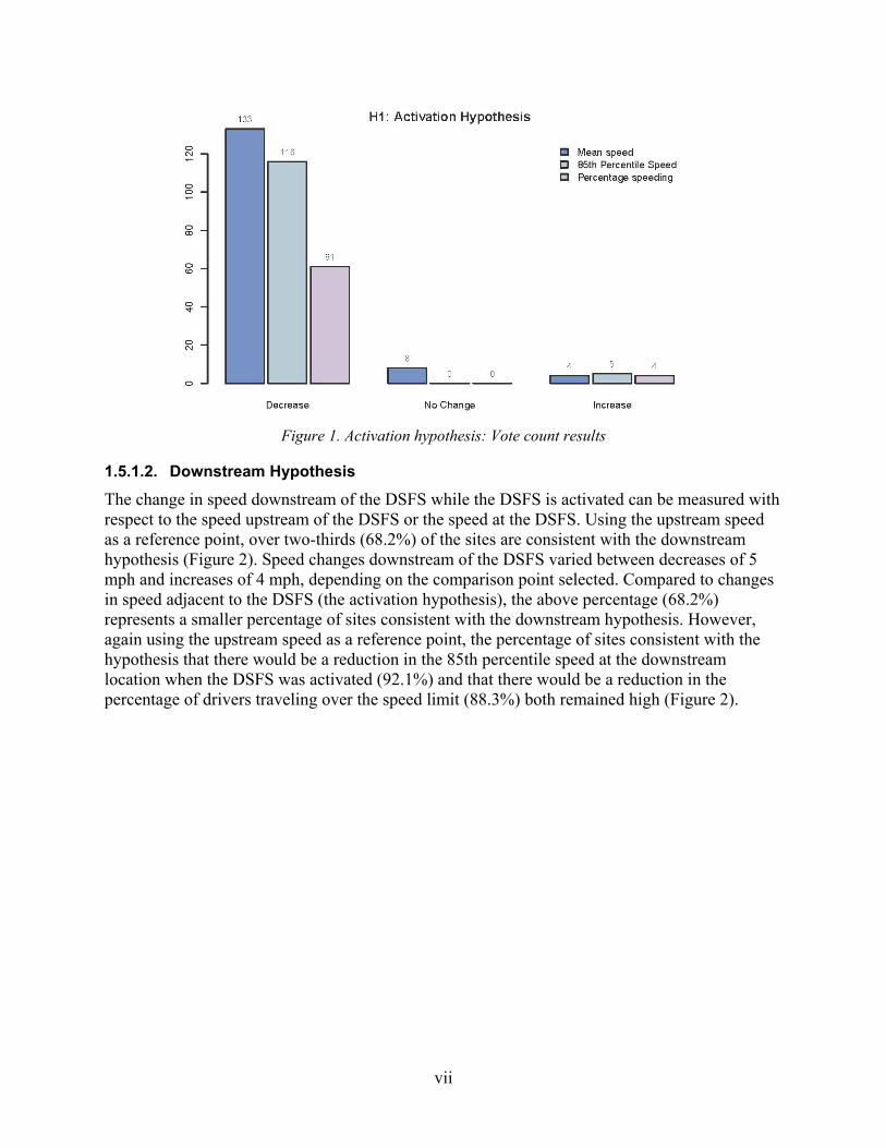
Out of 145 statistical evaluations of the decrease in mean speed at the DSFSs, 133 showed significant decreases, 8 showed no change, and 4 showed increases (Figure 1). The results at the overwhelming majority of sites, 92 percent, were consistent with the activation hypothesis that the speed would decrease at the DSFS. The meta-analysis was consistent with the vote count results. Overall, significant reductions of 2 to 4 mph at the DSFS were estimated across all vehicle types in the different contexts assessed. Although there were fewer analyses of changes in the 85th percentile speed and changes in the percentage of drivers traveling over the speed limit, in both cases the number of sites consistent with the hypothesis that there would be a reduction was clearly much larger than the alternative hypothesis (Figure 1).

vii

Figure 1. Activation hypothesis: Vote count results

1.5.1.2. Downstream Hypothesis

The change in speed downstream of the DSFS while the DSFS is activated can be measured with respect to the speed upstream of the DSFS or the speed at the DSFS. Using the upstream speed as a reference point, over two-thirds (68.2%) of the sites are consistent with the downstream hypothesis (Figure 2). Speed changes downstream of the DSFS varied between decreases of 5 mph and increases of 4 mph, depending on the comparison point selected. Compared to changes in speed adjacent to the DSFS (the activation hypothesis), the above percentage (68.2%) represents a smaller percentage of sites consistent with the downstream hypothesis. However, again using the upstream speed as a reference point, the percentage of sites consistent with the hypothesis that there would be a reduction in the 85th percentile speed at the downstream location when the DSFS was activated (92.1%) and that there would be a reduction in the percentage of drivers traveling over the speed limit (88.3%) both remained high (Figure 2).

viii

Figure 2. Downstream hypothesis: Vote count results

1.5.1.3. Deactivation Hypothesis

There were many fewer sites that reported information relevant to the deactivation hypothesis. The change in speed at the DSFS after deactivation can be measured relative to the DSFS sensor before activation or relative to the DSFS during activation. For the sites that measured the speed at the DSFSs after deactivation relative to the speed at the DSFS sensor before activation, all three showed significant decreases in speed. The magnitude of the mean speed change following DSFS removal varied between a decrease of 2 mph and increase of 1 mph, depending on the point of comparison used (the upstream speed before activation or the speed at the DSFS during activation). A decrease would be expected at the DSFS after deactivation relative to the upstream speed before activation if there was a continuing effect of the activation of the DSFS on the speed of the drivers, even following the removal of the sign.

1.5.2. Safety Focus The major vote count and meta-analysis findings for the five safety focal points are presented below as they bear on an evaluation of reductions in mean speed at the DSFS (the activation hypothesis). Results that are more detailed are presented in the literature review and the meta-analysis.

1.5.2.1. Work Zones

In work zones drivers are required to increase their attention not only to address the reduced speed of other vehicles, but also to address the added dangers of construction equipment, roadway design and markings, and pedestrian activity. The literature review found that 45 of 52 sites showed a significant decrease in speeds in work zones when DSFSs were installed, with mean speed reductions at the DSFS during activation of 2.75 mph being estimated in the meta-analysis.2

2 This reduction was estimated under Hypothesis 1A; activation effect normalized.

ix

1.5.2.2. School Zones

School zones showed a similar effectiveness for DSFS, with 24 of 28 sites showing significant reductions in mean vehicle speed at the DSFSs during sign activation. Speed reductions at the DSFS of 3.21 mph were estimated overall in school zones across all vehicle types, during DSFS activation.3 Studies found that speeds were reduced in school zones at the DSFS during activation for time periods of up to 12 months (O'Brien & Simpson, 2012), and by up to 9 mph (Ullman & Rose, 2005).

1.5.2.3. Transition Zones

Rural roads are the most dangerous roadway functional class in terms of speeding-related fatal crashes, with 41 percent of all speeding-related fatal crashes in 2018 (National Center for Statistics and Analysis, 2020) occurring on rural non-interstate roads. As drivers transition from rural roads to more densely settled areas, the required reductions in speed may be substantial. DSFS installations were effective in significantly reducing vehicle speeds at the DSFSs during activation in all 29 sites that examined their effect in transition zones, with speeds reductions estimated of 2.79 mph.4

1.5.2.4. Curves

Horizontal curves require the full attention of drivers, with some sites showing that longer reaction times are required to maintain safe vehicle operation on curves (Tribbett et al, 2000). DSFSs are effective in reducing speeds in this context, with all 29 sites that assessed mean speeds presenting significant reductions at the DSFS during activation. The meta-analysis estimated that speed reductions were 2.27 mph overall along curves.5

1.5.3. Vehicle Type The activation hypothesis was also evaluated for different classes of vehicles and the results suggest that vehicle type in addition to safety focus is an important consideration in measuring DSFS effectiveness. Across all of the safety focal points, passenger cars demonstrated larger reductions in mean vehicle speed at the DSFS than trucks. Considering just the effect of DSFS activation, the magnitude of the speed decrease for passenger cars was estimated as approximately double (4.7 mph) that of trucks (2.9 mph).6

3 This reduction was estimated under Hypothesis 1B; activation effect at the site of the DSFS. 4 This reduction was estimated under Hypothesis 1A; activation effect normalized. 5 This reduction was estimated under Hypothesis 1A; activation effect normalized. 6 This reduction was estimated under Hypothesis 1B; activation effect at the site of the DSFS.

x

1.6. Annotated Bibliography Finally, an annotated bibliography (Volume II) presents the details of each of the 43 publications reviewed in a consistent format, allowing an in-depth examination of the sign types, study designs, and unique characteristics of each study. We begin each review of an article with information on the study identifying information, relevance screening, and quality screening. We continue the review with a simple list of information relevant to the study, in five categories:

1. What hypotheses were evaluated;

2. What dependent variables were used to evaluate the hypotheses;

3. What were the results of those evaluations;

4. What were the characteristics of the study the practitioner needs to know to implement the DSFS in a particular setting, and

5. What are the aspects of the experimental design the researcher needs to know to evaluate the goodness of the study?

We have already discussed the first three of these categories. Details of a study that a practitioner needs to know to determine whether the study is relevant includes information such as:

• safety focus,

• classes of vehicles,

• posted speeds,

• type of DFS display,

• level of service,

• roadway type,

• roadway environment,

• presence of sidewalks, and

• sensor type.

Details of the study a researcher needs to know to evaluate the quality of or conduct a study include

• sensor positions;

• timing of the speed measurements prior to, during, and after activation of the DSFS; and

• experimental design.

xi

1.7. Discussion and Limitations There are several factors that must be considered when interpreting the results, the primary one of which is the way in which each of the three hypotheses are evaluated. We can best make this clear by way of an example (a complete discussion is included in Section 3.4, Volume I). As an example, we will choose the activation hypothesis.

First, the activation hypothesis can be directly tested as the change in vehicle speeds at the location where the DSFS will be installed, comparing the speeds of cars prior to installation of a DSFS (Car 1, 56 mph) to the speeds of cars when the sign is installed and active (Car 2, 46 mph) (Figure 3). Here there is a reduction of 10 mph. We refer to this as the “same site” measurement. This measure is commonly made in the literature, and is adequate for a considering, in general, how much a DSFS can reduce driver speed. One consideration, however, is that roadway conditions may have changed between the two time points that are measured, so vehicle speeds may differ for reasons other than the DSFS installation.

46

56

Figure 3. Activation hypothesis, same site. (Car 1 before activation, Car 2 during activation)

There are three ways to evaluate the activation hypothesis. To meaningfully interpret our findings on the activation hypothesis, one needs to understand the three different ways one can evaluate this hypothesis. Researchers generally choose only one way of evaluating the hypothesis and do not mention the alternatives or the limitations of the one that they choose.

An alternative method that studies have used to address the activation hypothesis is to measure speeds during the same trip, comparing vehicle speeds upstream of the site of DSFS installation (Car 2 at position before DSFS, 56 mph) to speeds adjacent to the DSFS (same car at DSFS, 46 mph) (Figure 4). This example also shows a speed reduction of 10 mph. As with the “same site” measurement, this “same trip” measurement method also may include changes in speed driven by factors besides the DSFS installation. This is particularly true since DSFSs are installed at sites where vehicle speeds are expected to decrease, such as prior to school zones or along horizontal curves. Thus this “same trip” measurement of the activation hypothesis is expected to only partly reflect the effect of the DSFS itself. Both these first two measures of the activation

xii

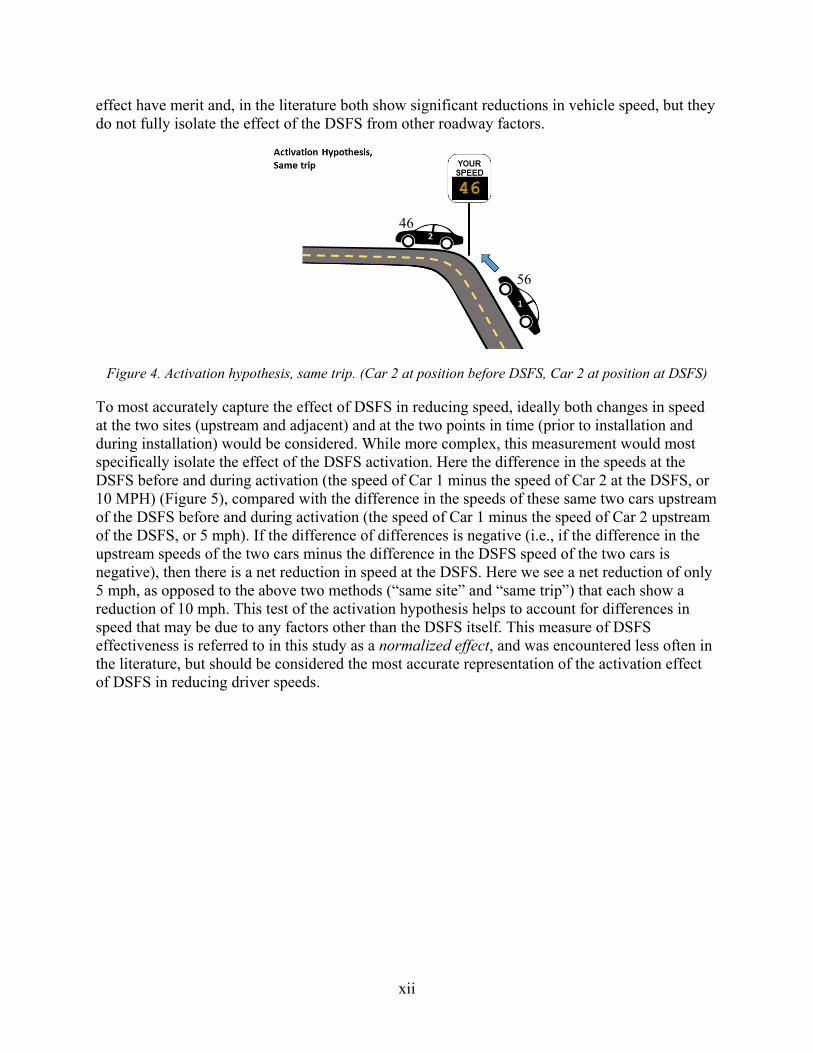
effect have merit and, in the literature both show significant reductions in vehicle speed, but they do not fully isolate the effect of the DSFS from other roadway factors.

46

56

Figure 4. Activation hypothesis, same trip. (Car 2 at position before DSFS, Car 2 at position at DSFS)

To most accurately capture the effect of DSFS in reducing speed, ideally both changes in speed at the two sites (upstream and adjacent) and at the two points in time (prior to installation and during installation) would be considered. While more complex, this measurement would most specifically isolate the effect of the DSFS activation. Here the difference in the speeds at the DSFS before and during activation (the speed of Car 1 minus the speed of Car 2 at the DSFS, or 10 MPH) (Figure 5), compared with the difference in the speeds of these same two cars upstream of the DSFS before and during activation (the speed of Car 1 minus the speed of Car 2 upstream of the DSFS, or 5 mph). If the difference of differences is negative (i.e., if the difference in the upstream speeds of the two cars minus the difference in the DSFS speed of the two cars is negative), then there is a net reduction in speed at the DSFS. Here we see a net reduction of only 5 mph, as opposed to the above two methods (“same site” and “same trip”) that each show a reduction of 10 mph. This test of the activation hypothesis helps to account for differences in speed that may be due to any factors other than the DSFS itself. This measure of DSFS effectiveness is referred to in this study as a normalized effect, and was encountered less often in the literature, but should be considered the most accurate representation of the activation effect of DSFS in reducing driver speeds.

xiii

56

46

56

61

Figure 5. Activation hypothesis, normalized

Other factors must also be considered when interpreting the results from a given study beside the exact hypotheses that were evaluated. We describe these factors in the literature review. They include, as noted above, the DSFS implementation characteristics (Section 3.6, Volume I) and the study design characteristics (Section 3.7, Volume I). Importantly, for every study in the literature review where a result was not consistent with the activation hypothesis and mean speed was the dependent measure, the reasons why such might have been the case are described. The simple vote count is just that, a vote count, and does not reflect the subtleties inherent in some studies. For example, we see in some studies that the vehicle speeds were already at or below the posted speed limit before the installation of the DSFS. In such studies, there is no reason to expect an effect of DSFS on a reduction in the vehicle speed and, indeed, there was none.

1.8. Summary By reviewing results and re-analyzing the data from the published literature (Volume I), the vote count and meta-analysis show that DSFSs are effective in reducing average vehicle speeds in all cases with sufficient data, as indicated either by the vote count or meta-analysis. The overall speed reductions of 4 mph for passenger cars at the DSFS can lead to substantial reductions in speeding-related crashes, reducing the human toll of fatal crashes. The annotated bibliography (Volume II) provides a summary of each study, with index tables to allow readers to quickly find relevant studies supporting this review.

1

2. Introduction

2.1. Background Speeding-related crashes continue to be a serious problem. Over the last decade, more than a quarter (26% in 2019) of all fatal crashes have been speeding-related (NCSA, 2021). NHTSA’s 2011 National Survey of Speeding Attitudes and Behaviors found that 30 percent of drivers were regular speeders and another 40 percent of drivers sped at least some of the time (Schroeder et al., 2013). In this same survey, the most widely approved countermeasure for speeding were DSFSs. The use of these signs was supported by 87 percent of speeders and 91 percent of sometime-speeders. Similarly, focus groups in NHTSA’s Motivations for Speeding study were also very supportive of DSFSs (Richard et al., 2013).

There have been many studies focusing on the effectiveness of DSFSs in reducing vehicle speeds. These studies vary substantially in roadway context, design, and study goal. An initial scan of the literature by NHTSA indicated that the studies focusing on DSFSs have included conditions with varying safety focal points (roadway departures, pedestrians, intersections, work zones), roadway types (collector, arterial, interstate, local), speed limits (from 25 to 65 mph), DSFS characteristics (e.g., stationary versus mobile units), and locations (urban, suburban, rural). At least one study looked at the use of DSFSs in conjunction with speed enforcement (Bloch & Automobile Club of Southern California, 2007). There was also at least one literature synthesis (Donnell & Cruzado, 2007) that covered 12 research studies on the effectiveness of DSFSs. Although most studies that were reviewed showed reductions in both mean speeds and 85th percentile speeds while the DSFSs are deployed, with one study (Tribbett et al., 2000) showing a reduction in crashes, the results were mixed, with some studies showing no reduction in speed and others an actual increase in speed.

It is important to keep in mind throughout this report that reductions in speed of even a few miles an hour can have a large impact on fatalities and injuries to pedestrians (Kloeden et al., 1997). For example, at relatively low speeds the risk of severe injury for 30-year-old pedestrians decreases from 50 percent to 25 percent as the speed at impact decreases by 6.5 mph from 33.5 mph to 26.0 mph (Tefft, 2011). The risk of severe injury for 70-year-old pedestrians decreases from 81 percent to 57 percent when the speeds at impact are decreased similarly. At slightly higher speeds, the risk of death for 30-year-olds decreases from 50 percent to 37 percent as the speed at impact decreases by 4 mph from 44.5 mph to 40.5 mph. The risk of death for 70-year-olds decreases from 81 percent to 71 percent as the speed at impact decreases by the same amount. Reductions in speed of even 4 to 6 mph can be of large practical significance when it comes to reducing the frequency of severe injuries and fatalities.

2.1.1. Reductions in Speed at the DSFS Location: Activation Hypothesis There are three ways to evaluate the activation hypothesis. To interpret meaningfully our findings on the activation hypothesis, one needs to understand the three different ways one can evaluate this hypothesis. Researchers generally choose only one way of evaluating the hypothesis and do not mention the alternatives or the limitations of the one that they do choose. First, the activation hypothesis can be directly tested as the change in vehicle speeds at a given location, comparing speeds prior to installation of a DSFS (Car 1, 56 mph) to speeds when the sign is installed and active (Car 2, 46 mph) (Figure 6). Here there is a reduction of 10 mph. This measure is commonly made in the literature, and is adequate for a considering, in general, how

2

much a DSFS can reduce driver speed. One consideration, however, is that roadway conditions may have changed between the two time points that are measured, so that vehicle speeds may differ for reasons other than the DSFS installation.

46

56

Figure 6. Activation hypothesis, same site

An alternative method that studies have used to address the activation hypothesis is to measure speeds during the same trip, comparing vehicle speeds upstream of the site of DSFS installation (Car position 1, 56) to speeds adjacent to the DSFS (Car position 2, 46) (Figure 7). This example also shows a speed reduction of 10 mph. As with the “same site” measurement, this measurement method also may include changes in speed driven by factors besides the DSFS installation. This is particularly true since DSFS are installed at sites where vehicle speeds are expected to decrease, such as prior to a school zone or along a horizontal curve. Thus this “same trip” measurement of the activation hypothesis is expected to only partly reflect the effect of the DSFS itself. Both of these first two measures of the activation effect have merit and, in the literature, both show significant reductions in vehicle speed, but they do not fully isolate the effect of the DSFS from other roadway factors.

46

56

Figure 7. Activation hypothesis, same trip

3

To most accurately capture the effect of DSFS in reducing speed, ideally both changes in speed at the two sites (upstream and adjacent) and at the two points in time (prior to installation and during installation) would be considered. While more complex, this measurement would most specifically isolate the effect of the DSFS activation. Here the difference in the speeds at the DSFS before and during activation (the speed of Car 4 minus the speed of Car 2 (Figure 8. activation hypothesis, normalized, compared with the difference in the speeds upstream of the DSFS before and during activation (the speed of Car 3 minus the speed of Car 1). If the difference of differences is negative, then there is a net reduction in speed at the DSFS. Here we see a net reduction of only 5 mph, as opposed to the above two methods that each show a reduction of 10 mph. This test of the activation hypothesis helps to account for differences in speed that may be due to any factors other than the DSFS itself. This measure of DSFS effectiveness is referred to in this study as a normalized effect, and was encountered less often in the literature, but should be considered the most accurate representation of the activation effect of DSFS in reducing driver speeds.

46

56 56

61

Figure 8. Activation hypothesis, normalized

2.1.2. Reductions in Speed Downstream of the DSFS: Downstream Hypothesis Safety officials may also consider using a DSFS to reduce speeds at a downstream location. For instance, it may be desired to begin tapering vehicle speeds well upstream of a transition zone between a rural highway and a more densely settled area. In this case, considering the downstream hypothesis would be appropriate. If the sign is placed too far upstream of the location of interest, vehicle speeds may recover to prior levels, so assessing the distance between the sign and the measurement location is critical. Just as for the activation hypothesis, considerations of the baseline comparison case are important, and in the literature both comparisons at the same time (Figure 9) and same site are presented. The downstream hypothesis has more variations than the activation hypothesis, since it is possible to consider both the site adjacent to the DSFS or upstream of the DSFS as baseline comparisons. These considerations are discussed further in the literature review and meta-analysis sections of this report.

4

Location of interest

Figure 9. Downstream hypothesis, same trip.

With respect just to reductions in speed downstream of the DSFS, using the upstream speed as the baseline, over two-thirds (68.2%) of the studies are consistent with the hypothesis that there would be a reduction in the mean speed downstream of the DSFS during the activation of the DSFS (H2). Compared to changes in speed adjacent to the DSFS (H1), this represents a smaller percentage of studies. However, the percentage of studies consistent with the hypothesis that there would be a reduction in the 85th percentile speed at the downstream location when the DSFS was activated (92.1%) and that there would be a reduction in the percentage of drivers traveling over the speed limit (88.3%) both remained high.

2.1.3. Reductions in Speed After Deactivation of the DSFS: Deactivation Hypothesis Finally, safety officials may consider temporarily installing a DSFS, for example, as part of a mobile operation in a work zone or as a test case to evaluate DSFS effectiveness. Upon removal of the DSFS, it is possible that a “halo effect” of continued reductions in driver speed may be observed. Some authors have tested this deactivation hypothesis. As with the downstream hypothesis, there are number of combinations of measurement in time (Figure 10) and space that are possible. For deactivation effects as shown in Figure 10, the published literature indicates that these halo effects can occur, although too few studies have been conducted to assess the statistical significance of this effect.

5

Figure 10. Deactivation hypothesis, same time. Removed DSFS indicated in grey.

2.2. Objectives of Study Given the large number of previous studies, end users in the highway safety community are faced with the challenge of sifting through the existing studies to locate appropriate research that addresses their needs. To reduce that burden, the Volpe National Transportation Systems Center (Volpe) was asked to conduct a comprehensive review of the existing literature on DSFS from 2000 to the present, produce an annotated bibliography of all studies found, and undertake a systematic and quantitative review of these studies, including a meta-analysis. This report aims to provide an important resource for both highway safety practitioners interested in reducing speeding and speeding-related crashes and researchers interested in doing further research on this important and widely accepted traffic safety countermeasure.

The remainder of this report is divided into three sections: the literature review (Volume I, Section 3), the meta-analysis (Volume I, Section 4), and the annotated bibliography (Volume II). Material in these sections is necessarily linked and we will make clear the interconnections where it is important to do such.

6

3. Literature Review

3.1. Literature Review Summary Speed has long been known to be a major contributor to crashes. This report addresses the effect that DSFSs can have on lowering speeds. The Volpe National Transportation Systems Center undertook a literature search for studies of DSFS effectiveness, focusing on domestic publications that reported changes in speed in terms of mean speed, 85th percentile speed, or percentage of vehicles in excess of posted speed limits. For each study that met the initial relevance and quality screening criteria, a detailed review was written and data were collected. These reviews are included in the annotated bibliography in Volume II. The data were used for the meta-analysis in Section 4 of this volume.

A total of 108 national and international publications were identified in the initial literature search. Focusing on the domestic studies, 77 publications were reviewed, of which 43 passed the relevance and quality screening.

This literature review summarizes the results of each publication using a vote-counting approach. A single publication can include more than one study, each of which can contain measurements for more than one DSFS site. A total of 725 sites were included in this review. Vote-counting here refers to summing the number of sites across all studies that show significant support for each outcome of the three hypotheses: the activation hypothesis -- the change in the mean speed at the DSFS when it was activated (labeled here as H1), the downstream hypothesis -- the change in the mean speed downstream of the DSFS when the DSFS is activated (H2), and the deactivation hypothesis -- the change in the mean speed at the DSFS after it is activated (H3). Vote counts are given for the change in the mean speed, the 85th percentile speed, and the percentage of drivers traveling over the posted speed limit for each of the three hypotheses.

In this summary of the literature review, we report only on the vote counts for mean speed; results for 85th percentile speed and percent of drivers speeding are found in the literature review. With respect to the change in the mean speed at the DSFS when it was activated (H1), measurements for 145 separate sites were reported. Of these, 133 were consistent with decreases in speed at the DSFS when it was activated; 8 showed no change; and 4 showed increases. With respect to the change in the mean speed downstream of the DSFS when the DSFS was activated (H2), 88 separate analyses were reported. Sixty of these were consistent with decreases in the mean speed downstream of the DSFS, 22 showed no change, and 6 showed increases in speed. Finally, with respect to the change in the mean speed after the DSFS was deactivated (H3), 3 studies were found, all of which reported significant decreases in the mean vehicle speed.

Additionally, the report separates out for each safety focus (work zone, school zone, transition zone, horizontal curve, or straight section) the vote count for the three main hypotheses. Critically, the safety focus summary includes a discussion of why those studies that were not consistent with the hypotheses might have included elements in the installation of a DSFS that are things to avoid when implementing a DSFS.

The vote count shows only the number of studies that provide evidence consistent with or not consistent with a given hypothesis. One would also like to know the exact size of the reduction in speed in order to predict the effect on crashes (Tefft, 2011). The meta-analysis (Section 4) shows the quantitative reductions in speed to be expected under different circumstances, for each of the hypotheses tested.

7

We have referred above to three main hypotheses, because each of the main hypotheses (activation hypothesis, downstream hypothesis, and deactivation hypothesis) has several ways of being evaluated, based on where and when the vehicle speeds are measured. The literature review discusses in detail the rationale for the different ways in which each of the three main hypotheses were evaluated and points to the advantages and disadvantages of each different method.

Based on the positive results, as reported above, traffic engineers may decide that it is useful to implement a DSFS in a particular location or that further study is needed. Not surprisingly, each of the studies reviewed vary greatly in terms of how the DSFS is implemented and how the experimental evaluation of the effect of the DSFS is undertaken. These characteristics were recorded for each study and are discussed in the literature review as well. Taken together, these results provide traffic engineers with the information that they need for planning a successful DSFS installation and provide researchers with the information that they require in determining exactly how the effects of the DSFS were evaluated.

This report is the first systematic synthesis of the numerous hypotheses, dependent and implementation variables, and experimental design characteristics that have been reported in studies of the effects of DSFS. As such, we hope that it paves the way for some standardization in the reporting of the experimental studies. This standardization can make it easier for future researchers to understand exactly what was done in each study and undertake additional analyses or new studies.

We continue below with a discussion of

• Methods used in the literature search and vote count,

• Typology of the characteristics of the studies including:

o Three different hypotheses that were evaluated,

o Three dependent variables that were used to evaluate those hypotheses,

o Variables that define a DSFS implementation, and

o Different experimental designs that were used to evaluate the hypotheses, and

• Detailed report (vote count) of the effectiveness of DSFSs with each of the five different safety focal points for each of the three different hypotheses and three different dependent variables along with an in-depth discussion of those studies that showed no effect of the DSFS on the mean speed at the DSFS or an actual increase in speed at the DSFS after activation.

3.2. Literature Search Methods The search for documents that report the effect of DSFS on driver behavior was undertaken from March 9 to March 16, 2016, by Volpe and MIT library staff. A total of 108 national and international publications were identified. Focusing on domestic studies, 77 publications were reviewed, of which 43 passed the relevance and quality screening.

8

3.2.1. Search Words and Phrases The words and phrases used in the literature search were relevant to the project’s key research questions:

• How are DSFSs being used to regulate speed?

• What are the extant findings regarding the effectiveness of DSFSs?

Searches started with the keywords (including the word variations) listed in Group 1 in the box below (Table 1). If the number of items retrieved was too large with the keywords used from Group 1, then the search words from Group 1 were combined one at a time with the keywords listed in Group 2. Only one of the Group 1 terms met these criteria, “speed limit signs,” with over 2,660 records. Any of the search terms in the tables that ended in “s” were wildcards with *. Wildcards allow one to search for all variants of a term. For example, “warning sign*” includes “warning sign,” “warning signs,” and “warning signage.” The reader will notice that many keywords are placed into groups (e.g., speed contains a number of keywords). Where keywords were listed under a group term, only the subordinate keywords were used in searches. However, in the one case where a group term had no subordinate keywords, “Traffic Calming Measures,” it was used as the search term along with “Traffic Calming” (TRID, TRB’s database, uses traffic calming as a thesaurus term).

Table 1. Search Words

Group 1 Group 2 • Speed

o Dynamic speed display signs (DSDS)

o Speed display signs o Dynamic warning signs o Dynamic speed feedback signs

(DSFS) o Speed feedback signs o Driver feedback signs o Speed monitoring displays (SMD) o Speed displays o Speed display trailer o Dynamic displays o Speed warning signs o Variable message speed limit signs o Speed limit signs o Speed minders o Speed indicator device (SID) o Speed reduction treatments o Radar speed signs o Radar speed check signs o Photo-radar displays

• Curves o Dynamic curve warning signs o Advance curve warnings

• Traffic calming measures

• Locations o Curves o School zones o Work zones o Intersections o Transition zones

• Treatment effects o Speed reduction o Speed decreases o 85th percentile speed reductions

9

Seven extensive databases were searched: Transportation Research International Documentation (TRID), National Transportation Library, WorldCat, Academic Search Complete, PsychINFO, Web of Science, and Science Direct. Together, these databases provide a comprehensive coverage of academic and governmental transportation-related research.

3.2.2. Results of Search The search yielded 106 references, placed into different categories (Table 2). It was decided initially to review only domestic studies given the differences in roadway design, traffic regulations, and driving cultures around the world. This led to the exclusion of 30 studies; however, one of those studies had already been reviewed prior to the decision to focus on just domestic articles. This review is included in the annotated bibliography, but it was not used for the other components of this study. Of the 76 remaining domestic sources, 19 were redundant. For example, a study that appeared as a “proceedings” article with one set of authors and title might also appear as a journal article with different authors, different titles, or seemingly different content. Of the remaining 57 articles, 3 could not be located (retrieved from the URL or other internet searches), leaving 54 articles to be screened for relevance and quality.

Table 2. Summary of publications evaluated for literature review.

Decision Number Included 43 Data article (42) Review article (1) Redundant 19 International 29 No speed data 5 Sign not relevant to speeds 6 Not able to retrieve 3 Synthesis (included) 1 Total 106

The screening process was two-tiered. First, a study was reviewed for relevance. If it passed this screening, the study was then reviewed for quality. To measure study relevance, two questions were asked of a study, following a standard practice in systematic literature reviews (Cooper et al., 2009). The relevance criteria were as follows.

1. Is this study an empirical investigation of the effectiveness of DSFSs?

2. Is the outcome measure crashes, fatal crashes, and/or some function of traffic speeds?

In 6 of the studies, the signs that were used did not report driver speed. That left 49 studies to review for quality.

10

To measure the quality of the studies that made it through the relevance screening, three questions were asked of each study.

1. Were the study population and the context of the study well described?

2. Were the exposure variables valid implementations of the conditions that they were meant to represent?

3. Was the outcome variable both a reliable and valid measure of the outcome of interest?

In 5 of the studies no speed data were reported. That left 43 studies, one of which was a literature review. The literature review was not included in the set of 42 studies that were used for the vote count.

3.2.3. Types of Dynamic Feedback Signs Across these publications, different types of DSFSs were employed, including portable changeable message signs (PCMSs), speed monitoring displays (SMDs), and speed display trailers (SDTs). The configurations of signs and messages, which are included as part of a DSFS deployment, varied widely across installations. Examples of the types of configurations commonly encountered are presented in Appendix B (Volume II), and details on the configurations of signs in each publication are presented in the annotated bibliography (Volume II).

3.2.4. Article Review Template The 43 included articles were reviewed in detail and are included in a separate annotated bibliography (Volume II). Each review has four sections:

1. A list of the features of the study, including details on the implementation of the DSFS and the design of the study;

2. A summary of the study or studies included in the article;

3. A schematic diagram indicating the location of the speed sensors and DSFS as well as the geometry of the roadway where the treatment was applied at each site; and

4. A graphic of the DSFSs used.

A detailed description of each section is included in Appendix C of Volume II.

3.3. Vote Count Methods For each of the three hypotheses and each dependent variable, we counted the number of sites where a decrease, an increase, or no change in speed was noted. Complete descriptions of the hypotheses are described below in Section 3.4. We then present these summaries as a vote count (Koricheva & Gurevitch, 2016). In a vote count, the number of significant results for each alternative hypothesis is simply summed across studies. This type of review is quantitative in the sense that significant results are summed, but does not take into account the size of the effect (i.e., how many mph speeds were reduced as a result of the DSFS), the sample size, or the variability of the effect size. These factors require more data to consider and are included in the meta-analysis in Section 4.

11

The specifics of the vote count are as follows. Assume a study had n sites with one statistical evaluation at each site. Suppose that for a particular hypothesis and particular dependent variable, the results from m of the n sites were consistent with a particular hypothesis, m < n. Then, m votes were tallied as consistent with the hypothesis and n – m votes as not consistent with the hypothesis. The n – m were further partitioned into those that showed no change in speed and those that showed an increase in speed.

Consider a single hypothetical study. Suppose the mean speed was measured at the DSFS before activation and then again at the DSFS during activation (H1B, a particular variation of the DSFS activation hypothesis; see Section 3.4.1). Suppose there were 12 sites. Suppose significant reductions in speed were recorded at 9 of the 12 sites, no significance change in speeds were recorded at 2 sites, and an increase in speed was recorded at 1 site. Then, Volpe would add 9 votes as supporting the DSFS activation hypothesis (a reduction in speed at the DSFS when it is activated), 2 votes as showing no change in speed, and 1 vote as showing an increase in speed.

In the unusual case that several vehicle classes were measured at one site, these were counted separately. So, for example suppose there were 2 sites and the speed of both trucks and cars were recorded at both sites. Then, if the speeds were reduced at the DSFS for cars and there was no change for trucks, this would be recorded as 2 votes for a decrease and 2 votes for no change.

3.4. Hypotheses There are three major hypotheses evaluated in the studies. The DSFS activation hypothesis (H1) is used to evaluate the following question: At the location of the DSFS, are speeds reduced after the DSFS is activated? The DSFS downstream activation hypothesis (H2) answers the following question: Downstream of the DSFS, are speeds reduced after the DSFS is activated? The DSFS deactivation hypothesis (H3) answers the question: After removal of the DSFS, are speeds reduced at the DSFS from what they were when the DSFS was activated? Upon further inspection, it became clear that there were three different variations of H1, five different variations of H2, and five different variations of H3. Use of this typology would help future researchers by standardizing the terminology, facilitating the search for a study relevant to a hypothesis of particular interest.

3.4.1. Hypothesis 1: Activation Effect at DSFS There are three different variations on the activation hypothesis H1. These variations can lead to very different conclusions about the effectiveness of a DSFS. One might wish it were simply a matter of answering the question: Is the speed reduced or is it not reduced at the DSFS when the DSFS is activated? However, because studies often used different ways of answering this question, and because there are different ways of evaluating the hypothesis, it is important that the reader understand the different variations of the DSFS activation hypothesis.

First, consider the ideal measurement. To assess how the activation of a DSFS reduces driver speed, the ideal measurement would account for the change in vehicle speed from prior to the sign installation to during sign activation. The ideal measurement would also account for any change in the upstream speeds that occurred prior to the sign installation and during the sign installation. Such a measurement is given on the following page in Equation 1:

12

H1A: (𝐷𝐷𝐷𝐷𝐷𝐷𝐷𝐷𝐷𝐷𝐷𝐷𝐷𝐷𝐷𝐷𝐷𝐷𝐷𝐷 − 𝐵𝐵𝐵𝐵𝐵𝐵𝐵𝐵𝐷𝐷𝐵𝐵𝐷𝐷𝐷𝐷𝐷𝐷𝐷𝐷) − �𝐷𝐷𝐷𝐷𝐷𝐷𝐷𝐷𝐷𝐷𝐷𝐷𝑈𝑈𝑈𝑈𝑈𝑈𝑈𝑈𝑈𝑈𝑈𝑈𝑈𝑈𝑈𝑈 − 𝐵𝐵𝐵𝐵𝐵𝐵𝐵𝐵𝐷𝐷𝐵𝐵𝑈𝑈𝑈𝑈𝑈𝑈𝑈𝑈𝑈𝑈𝑈𝑈𝑈𝑈𝑈𝑈�

Equation 1

In Equation 1 the measured quantity is negative if the reduction in speed observed between measurements made at the DSFS before and during activation is larger than the change in speed observed upstream before and during activation.

This is made clear in Figure 11. Rows in the tables in the Required Data column represent locations of the sensor measuring speed (upstream of the DSFS, adjacent to the DSFS, or downstream of the DSFS), and column represent times during which the measurements of speed are made (before activation of the DSFS, during activation of the DSFS, or after deactivation of the DSFS). The first in Equation 1, in blue, is the difference that occurs in the speeds of the cells labelled B and A in Figure 11. The second value in Equation 1, in green, is the difference that occurs in the speeds of the cells labelled D and C in Figure 11. Note that the difference of differences is negative if there is a reduction in speed.

Hypothesis Code Hypotheses Speed Reduction Formula Required Data

H1A

Activation Effect at DSFS, normalized relative to upstream

(𝐷𝐷𝐷𝐷𝐷𝐷𝐷𝐷𝐷𝐷𝐷𝐷𝐷𝐷𝐷𝐷𝐷𝐷𝐷𝐷 − 𝐵𝐵𝐵𝐵𝐵𝐵𝐵𝐵𝐷𝐷𝐵𝐵𝐷𝐷𝐷𝐷𝐷𝐷𝐷𝐷) − �𝐷𝐷𝐷𝐷𝐷𝐷𝐷𝐷𝐷𝐷𝐷𝐷𝑈𝑈𝑈𝑈𝑈𝑈𝑈𝑈𝑈𝑈𝑈𝑈𝑈𝑈𝑈𝑈− 𝐵𝐵𝐵𝐵𝐵𝐵𝐵𝐵𝐷𝐷𝐵𝐵𝑈𝑈𝑈𝑈𝑈𝑈𝑈𝑈𝑈𝑈𝑈𝑈𝑈𝑈𝑈𝑈�

Timing

Before During After Lo

catio

n

Upstream C D

Adjacent A B

Downstream

H1B

Activation Effect at DSFS, relative to before

(𝐷𝐷𝐷𝐷𝐷𝐷𝐷𝐷𝐷𝐷𝐷𝐷𝐷𝐷𝐷𝐷𝐷𝐷𝐷𝐷 − 𝐵𝐵𝐵𝐵𝐵𝐵𝐵𝐵𝐷𝐷𝐵𝐵𝐷𝐷𝐷𝐷𝐷𝐷𝐷𝐷)

Before During After

Loca

tion

Upstream

Adjacent A B

Downstream

H1C

Activation Effect at DSFS, relative to upstream

�𝐷𝐷𝐷𝐷𝐷𝐷𝐷𝐷𝐷𝐷𝐷𝐷𝐷𝐷𝐷𝐷𝐷𝐷𝐷𝐷− 𝐷𝐷𝐷𝐷𝐷𝐷𝐷𝐷𝐷𝐷𝐷𝐷𝑈𝑈𝑈𝑈𝑈𝑈𝑈𝑈𝑈𝑈𝑈𝑈𝑈𝑈𝑈𝑈�

Before During After

Loca

tion

Upstream D

Adjacent B

Downstream

Figure 11. Hypotheses H1A, H1B, and H1C. The locations upstream, adjacent, and downstream are all relative to the DSFS.

13

Second, one can compare the speed at the DSFS during activation to the speed at the DSFS before activation. We can represent this quantitatively as the difference in the speed at the DSFS during the activation of the DSFS (𝐷𝐷𝐷𝐷𝐷𝐷𝐷𝐷𝐷𝐷𝐷𝐷𝐷𝐷𝐷𝐷𝐷𝐷𝐷𝐷 ) and the speed at the DSFS before the activation of the DSFS ( 𝐵𝐵𝐵𝐵𝐵𝐵𝐵𝐵𝐷𝐷𝐵𝐵𝐷𝐷𝐷𝐷𝐷𝐷𝐷𝐷)7:

H1B: (𝐷𝐷𝐷𝐷𝐷𝐷𝐷𝐷𝐷𝐷𝐷𝐷𝐷𝐷𝐷𝐷𝐷𝐷𝐷𝐷 − 𝐵𝐵𝐵𝐵𝐵𝐵𝐵𝐵𝐷𝐷𝐵𝐵𝐷𝐷𝐷𝐷𝐷𝐷𝐷𝐷)

Equation 2

We refer to this as hypothesis H1B (measures made at same location at different times). This is made clear graphically in Figure 11. Note the result in Equation 2 is negative if there is a reduction in speed.

Third, one can compare the speed at the sensor upstream of the DSFS during activation of the DSFS with the speed at the DSFS during the activation of the DSFS (H1C; measures made at different locations at the same time). This appears in Figure 11 and is expressed quantitatively as:

H1C: �𝐷𝐷𝐷𝐷𝐷𝐷𝐷𝐷𝐷𝐷𝐷𝐷𝐷𝐷𝐷𝐷𝐷𝐷𝐷𝐷 − 𝐷𝐷𝐷𝐷𝐷𝐷𝐷𝐷𝐷𝐷𝐷𝐷𝑈𝑈𝑈𝑈𝑈𝑈𝑈𝑈𝑈𝑈𝑈𝑈𝑈𝑈𝑈𝑈�

Equation 3

Again, the difference is negative if there is a reduction in speed.

Either of the second and third measures has limitations. H1B does not control for differences in the upstream speed before and during activation. H1C does not control for differences in the speed before activation that may exist between the sensor upstream of the DSFS and at the DSFS. Algebraically, controlling for the differences in H1B leads to a quantity that is identical to what is obtained when one controls for the differences in H1C; either way results in H1A.

An example shows how these methods of assessing the activation effect of the DSFS differ in critical ways. Assume the following values for the speeds measured before and after the activation of the DSFS both upstream of the DSFS and adjacent to the DSFS:

• 𝐷𝐷𝐷𝐷𝐷𝐷𝐷𝐷𝐷𝐷𝐷𝐷𝐷𝐷𝐷𝐷𝐷𝐷𝐷𝐷 = 30

• 𝐵𝐵𝐵𝐵𝐵𝐵𝐵𝐵𝐷𝐷𝐵𝐵𝐷𝐷𝐷𝐷𝐷𝐷𝐷𝐷 = 40

• 𝐷𝐷𝐷𝐷𝐷𝐷𝐷𝐷𝐷𝐷𝐷𝐷𝑈𝑈𝑈𝑈𝑈𝑈𝑈𝑈𝑈𝑈𝑈𝑈𝑈𝑈𝑈𝑈 = 45

• 𝐵𝐵𝐵𝐵𝐵𝐵𝐵𝐵𝐷𝐷𝐵𝐵𝑈𝑈𝑈𝑈𝑈𝑈𝑈𝑈𝑈𝑈𝑈𝑈𝑈𝑈𝑈𝑈 = 50

Evaluating H1A we find a reduction in speed of 5 mph (Figure 12), evaluating H1B we find a reduction in speed of 10 mph, and evaluating H1C we find a reduction in speed of 15 mph. Any negative value for the change in speed is consistent with the desired outcome. However, the different ways of evaluating H1 could lead to large differences in the effect sizes computed in a meta-analysis.

7 Note that we could also have written 𝐷𝐷𝐷𝐷𝐷𝐷𝐷𝐷𝐷𝐷𝐷𝐷𝐷𝐷𝐷𝐷𝐷𝐷𝐷𝐷 as 𝐷𝐷𝐷𝐷𝐷𝐷𝐷𝐷𝐷𝐷𝐷𝐷𝐴𝐴𝐴𝐴𝐴𝐴𝑈𝑈𝐴𝐴𝑈𝑈𝐴𝐴𝑈𝑈 and 𝐵𝐵𝐵𝐵𝐵𝐵𝐵𝐵𝐷𝐷𝐵𝐵𝐷𝐷𝐷𝐷𝐷𝐷𝐷𝐷 as 𝐵𝐵𝐵𝐵𝐵𝐵𝐵𝐵𝐷𝐷𝐵𝐵𝐴𝐴𝐴𝐴𝐴𝐴𝑈𝑈𝐴𝐴𝑈𝑈𝐴𝐴𝑈𝑈 (see Figure 11).

14

Hypothesis Code

Hypotheses Speed Reduction Formula Required Data

H1A

Activation effect at DSFS, normalized relative to upstream

(𝐷𝐷𝐷𝐷𝐷𝐷𝐷𝐷𝐷𝐷𝐷𝐷𝐷𝐷𝐷𝐷𝐷𝐷𝐷𝐷 − 𝐵𝐵𝐵𝐵𝐵𝐵𝐵𝐵𝐷𝐷𝐵𝐵𝐷𝐷𝐷𝐷𝐷𝐷𝐷𝐷)−

�𝐷𝐷𝐷𝐷𝐷𝐷𝐷𝐷𝐷𝐷𝐷𝐷𝑈𝑈𝑈𝑈𝑈𝑈𝑈𝑈𝑈𝑈𝑈𝑈𝑈𝑈𝑈𝑈− 𝐵𝐵𝐵𝐵𝐵𝐵𝐵𝐵𝐷𝐷𝐵𝐵𝑈𝑈𝑈𝑈𝑈𝑈𝑈𝑈𝑈𝑈𝑈𝑈𝑈𝑈𝑈𝑈�

= −5

Timing

Before During After

Loca

tion

Upstream 50 45

Adjacent 40 30

Downstream

H1B

Activation effect at DSFS, relative to before

(𝐷𝐷𝐷𝐷𝐷𝐷𝐷𝐷𝐷𝐷𝐷𝐷𝐷𝐷𝐷𝐷𝐷𝐷𝐷𝐷 − 𝐵𝐵𝐵𝐵𝐵𝐵𝐵𝐵𝐷𝐷𝐵𝐵𝐷𝐷𝐷𝐷𝐷𝐷𝐷𝐷)= −10

Before During After

Loca

tion

Upstream

Adjacent 40 30

Downstream

H1C

Activation effect at DSFS, relative to upstream

�𝐷𝐷𝐷𝐷𝐷𝐷𝐷𝐷𝐷𝐷𝐷𝐷𝐷𝐷𝐷𝐷𝐷𝐷𝐷𝐷− 𝐷𝐷𝐷𝐷𝐷𝐷𝐷𝐷𝐷𝐷𝐷𝐷𝑈𝑈𝑈𝑈𝑈𝑈𝑈𝑈𝑈𝑈𝑈𝑈𝑈𝑈𝑈𝑈� = −15

Before During After

Loca

tion

Upstream 45

Adjacent 30

Downstream

Figure 12. Quantitative example: Activation hypotheses H1.

3.4.2. Hypothesis 2: Downstream Activation Effect To test whether vehicles reduce speeds downstream of the DSFS, there are now three possible comparisons: the downstream sensor before activation with the downstream sensor during activation; the upstream sensor during activation with the downstream sensor during activation, and the DSFS sensor during activation with the downstream sensor during activation.

Consider the first two comparisons: the speed at the downstream sensor before activation with the speed at the downstream sensor during activation (labeled H2B) and the speed at the upstream sensor during activation with the speed at the downstream sensor during activation (H2C). If we subtract the comparison sensor speed from the downstream sensor speed during activation the result should be negative. Moreover, when we control either for changes in speed that might have occurred simply as a function of differences in the time of the two measurements that are used to evaluate H2B or for the changes in speed that occurred simply as a function of differences in the locations of the two measurements that are used to evaluate H2C, we get one and the same algebraic quantity (which we label as H2A). These three hypotheses and their corresponding formulas are represented in Figure 13 (H2A, H2B, and H2C, parallels of H1A, H1B and H1C). It is clear from the computations why, as before, it is important to be certain about just what hypothesis one is evaluating. Any computation that produces a significant negative result is associated with a favorable outcome.

15

Hypothesis Code Hypotheses Speed Reduction Formula Required Data

H2A

Activation Effect Downstream of DSFS, normalized relative to upstream

(𝐷𝐷𝐷𝐷𝐷𝐷𝐷𝐷𝐷𝐷𝐷𝐷𝐷𝐷𝐷𝐷𝐷𝐷𝐴𝐴𝑈𝑈𝑈𝑈𝑈𝑈𝑈𝑈𝑈𝑈𝑈𝑈− 𝐵𝐵𝐵𝐵𝐵𝐵𝐵𝐵𝐷𝐷𝐵𝐵𝐷𝐷𝐷𝐷𝐷𝐷𝐴𝐴𝑈𝑈𝑈𝑈𝑈𝑈𝑈𝑈𝑈𝑈𝑈𝑈) −

�𝐷𝐷𝐷𝐷𝐷𝐷𝐷𝐷𝐷𝐷𝐷𝐷𝑈𝑈𝑈𝑈𝑈𝑈𝑈𝑈𝑈𝑈𝑈𝑈𝑈𝑈𝑈𝑈 −𝐵𝐵𝐵𝐵𝐵𝐵𝐵𝐵𝐷𝐷𝐵𝐵𝑈𝑈𝑈𝑈𝑈𝑈𝑈𝑈𝑈𝑈𝑈𝑈𝑈𝑈𝑈𝑈� = -5

Timing

Before During After

Loca

tion

Upstream 50 45

Adjacent

Downstream 35 25

H2B

Activation Effect Downstream of DSFS, relative to before

(𝐷𝐷𝐷𝐷𝐷𝐷𝐷𝐷𝐷𝐷𝐷𝐷𝐷𝐷𝐷𝐷𝐷𝐷𝐴𝐴𝑈𝑈𝑈𝑈𝑈𝑈𝑈𝑈𝑈𝑈𝑈𝑈− 𝐵𝐵𝐵𝐵𝐵𝐵𝐵𝐵𝐷𝐷𝐵𝐵𝐷𝐷𝐷𝐷𝐷𝐷𝐴𝐴𝑈𝑈𝑈𝑈𝑈𝑈𝑈𝑈𝑈𝑈𝑈𝑈) = −10

Before During After

Loca

tion

Upstream

Adjacent

Downstream 35 25

H2C

Activation Effect Downstream of DSFS, relative to upstream

�𝐷𝐷𝐷𝐷𝐷𝐷𝐷𝐷𝐷𝐷𝐷𝐷𝐷𝐷𝐷𝐷𝐷𝐷𝐴𝐴𝑈𝑈𝑈𝑈𝑈𝑈𝑈𝑈𝑈𝑈𝑈𝑈− 𝐷𝐷𝐷𝐷𝐷𝐷𝐷𝐷𝐷𝐷𝐷𝐷𝑈𝑈𝑈𝑈𝑈𝑈𝑈𝑈𝑈𝑈𝑈𝑈𝑈𝑈𝑈𝑈� = −20

Before During After

Loca

tion

Upstream 45

Adjacent

Downstream 25

H2A'

Activation Effect Downstream of DSFS, normalized relative to adjacent

(𝐷𝐷𝐷𝐷𝐷𝐷𝐷𝐷𝐷𝐷𝐷𝐷𝐷𝐷𝐷𝐷𝐷𝐷𝐴𝐴𝑈𝑈𝑈𝑈𝑈𝑈𝑈𝑈𝑈𝑈𝑈𝑈− 𝐵𝐵𝐵𝐵𝐵𝐵𝐵𝐵𝐷𝐷𝐵𝐵𝐷𝐷𝐷𝐷𝐷𝐷𝐴𝐴𝑈𝑈𝑈𝑈𝑈𝑈𝑈𝑈𝑈𝑈𝑈𝑈) −

(𝐷𝐷𝐷𝐷𝐷𝐷𝐷𝐷𝐷𝐷𝐷𝐷𝐷𝐷𝐷𝐷𝐷𝐷𝐷𝐷 − 𝐵𝐵𝐵𝐵𝐵𝐵𝐵𝐵𝐷𝐷𝐵𝐵𝐷𝐷𝐷𝐷𝐷𝐷𝐷𝐷)= 0

Before During After

Loca

tion

Upstream

Adjacent 40 30

Downstream 35 25

H2C'

Activation Effect Downstream of DSFS, relative to adjacent

(𝐷𝐷𝐷𝐷𝐷𝐷𝐷𝐷𝐷𝐷𝐷𝐷𝐷𝐷𝐷𝐷𝐷𝐷𝐴𝐴𝑈𝑈𝑈𝑈𝑈𝑈𝑈𝑈𝑈𝑈𝑈𝑈− 𝐷𝐷𝐷𝐷𝐷𝐷𝐷𝐷𝐷𝐷𝐷𝐷𝐷𝐷𝐷𝐷𝐷𝐷𝐷𝐷) = −5

Before During After

Loca

tion

Upstream

Adjacent 30

Downstream 25

Figure 13. Quantitative example: Downstream hypotheses H2.

Finally, consider the third comparison, the speed at the adjacent sensor during activation with the speed at the downstream sensor during activation (H2C′). The desirable outcome is no change in the speed at the downstream sensor, the hope being that the effect of the DSFS will not dissipate with distance from the DSFS. If we control for the differences in speed that might occur simply because of a difference in location, we get the normalized quantity we label as H2A′. These last hypotheses and their corresponding formulas are represented in Figure 13 (H2A′ and H2C′).

Note that we can normalize H2B either with respect to the changes in speed across time at the upstream sensors or the changes in speed across time at the adjacent sensors. The normalized quantity, H2A, for H2B with respect to changes in speed across time at the upstream sensors,

16

will not necessarily be the same as the normalized quantity, H2A′, for H2B with respect to the changes in speed across time at the adjacent sensors (compare the speed reduction formula in Row 1 of Figure 13 with the speed reduction formula in Row 4 of the same figure). Also note that H2B is the same as H2B′ and therefore it is not listed in Figure 13.

An example can help make clear of the difference between H2 unprimed and H2 primed hypotheses (Figure 13). Note that the results are all negative for the three variations of H2: H2A, H2B and H2C. If the result were negative and significant, the result is consistent with the hypothesis that there is an effect of the activation of the DSFS on the downstream sensor when the comparison point is the upstream sensor. However, look now at the results for H2 primed where the comparison point is adjacent to the DSFS. If we look only at the difference in the speed of the vehicles at the DSFS and the downstream sensor while the DSFS is activated, then we see a reduction of 5 mph (H2C′). If we look only at the difference in speed at the downstream sensors across time we see a reduction in speed of 10 mph (H2B or H2B′). However, consider the normalized versions of H2B′ and H2C′, what we refer to as H2A′. In this example, no change in speed is observed.

Finally, we should note that, as discussed above, the normalization of H2B with respect to the upstream sensors shows a reduction in speed of 4 mph (H2A = -5) whereas the normalization of H2B with respect to the adjacent sensors shows no change in speed (H2A′ = 0). Both answers are correct as normalizations of H2B (a reduction in speed of 5 mph, H2A, or no reduction in speed, H2A′), they just reference different questions or hypotheses.

3.4.3. Hypothesis 3: Deactivation Effect at the DSFS Just as there are three pairwise comparisons for the downstream sensor, so too there are three pairwise comparisons for evaluating the effect of the deactivation of the DSFS: the speed at the DSFS after its deactivation compared to the speed at the DSFS before its activation; the speed upstream of the DSFS after its deactivation with the speed at the DSFS after its deactivation; and the speed at the DSFS during the activation to the speed at the DSFS after its activation. Note that as with hypothesis 2, for hypothesis 3 the first two pairwise comparisons should be negative if the speed at the DSFS after its deactivation is slower than it was before its activation. Similarly, the third pairwise comparison should show no change if the speed at the DSFS after its deactivation does not increase from what the speed was at the DSFS during its activation. Again, there are different ways of making the computations with the un-normalized (H2B, H2C, H2B′) and normalized (H3A, H3A′) hypotheses (Figure 14).

17

Hypothesis Code Hypotheses Speed Reduction Formula Required Data

H3A

Deactivation effect at DSFS, normalized relative to upstream

(𝐴𝐴𝐵𝐵𝐴𝐴𝐵𝐵𝐷𝐷𝐷𝐷𝐷𝐷𝐷𝐷𝐷𝐷 − 𝐵𝐵𝐵𝐵𝐵𝐵𝐵𝐵𝐷𝐷𝐵𝐵𝐷𝐷𝐷𝐷𝐷𝐷𝐷𝐷) −

�𝐴𝐴𝐵𝐵𝐴𝐴𝐵𝐵𝐷𝐷𝑈𝑈𝑈𝑈𝑈𝑈𝑈𝑈𝑈𝑈𝑈𝑈𝑈𝑈𝑈𝑈−𝐵𝐵𝐵𝐵𝐵𝐵𝐵𝐵𝐷𝐷𝐵𝐵𝑈𝑈𝑈𝑈𝑈𝑈𝑈𝑈𝑈𝑈𝑈𝑈𝑈𝑈𝑈𝑈�

= −10

Timing

Before During After

Loca

tion Upstream 50 55

Adjacent 40 35

Downstream

H3B

Deactivation effect at DSFS, relative to before

(𝐴𝐴𝐵𝐵𝐴𝐴𝐵𝐵𝐷𝐷𝐷𝐷𝐷𝐷𝐷𝐷𝐷𝐷 − 𝐵𝐵𝐵𝐵𝐵𝐵𝐵𝐵𝐷𝐷𝐵𝐵𝐷𝐷𝐷𝐷𝐷𝐷𝐷𝐷) = −5

Before During After

Loca

tion Upstream

Adjacent 40 35

Downstream

H3C

Deactivation effect at DSFS, relative to after

�𝐴𝐴𝐵𝐵𝐴𝐴𝐵𝐵𝐷𝐷𝐷𝐷𝐷𝐷𝐷𝐷𝐷𝐷 − 𝐴𝐴𝐵𝐵𝐴𝐴𝐵𝐵𝐷𝐷𝑈𝑈𝑈𝑈𝑈𝑈𝑈𝑈𝑈𝑈𝑈𝑈𝑈𝑈𝑈𝑈� = −20

Before During After

Loca

tion Upstream 55

Adjacent 35

Downstream

H3A′

Deactivation effect at DSFS, normalized relative to upstream

(𝐴𝐴𝐵𝐵𝐴𝐴𝐵𝐵𝐷𝐷𝐷𝐷𝐷𝐷𝐷𝐷𝐷𝐷 − 𝐷𝐷𝐷𝐷𝐷𝐷𝐷𝐷𝐷𝐷𝐷𝐷𝐷𝐷𝐷𝐷𝐷𝐷𝐷𝐷 ) −�𝐴𝐴𝐵𝐵𝐴𝐴𝐵𝐵𝐷𝐷𝑈𝑈𝑈𝑈𝑈𝑈𝑈𝑈𝑈𝑈𝑈𝑈𝑈𝑈𝑈𝑈 − 𝐷𝐷𝐷𝐷𝐷𝐷𝐷𝐷𝐷𝐷𝐷𝐷𝑈𝑈𝑈𝑈𝑈𝑈𝑈𝑈𝑈𝑈𝑈𝑈𝑈𝑈𝑈𝑈�

= −5

Before During After

Loca

tion Upstream 45 55

Adjacent 30 35

Downstream

H3B'

Deactivation effect at DSFS, relative to during

(𝐴𝐴𝐵𝐵𝐴𝐴𝐵𝐵𝐷𝐷𝐷𝐷𝐷𝐷𝐷𝐷𝐷𝐷 − 𝐷𝐷𝐷𝐷𝐷𝐷𝐷𝐷𝐷𝐷𝐷𝐷𝐷𝐷𝐷𝐷𝐷𝐷𝐷𝐷) = 5

Before During After

Loca

tion Upstream

Adjacent 30 35

Downstream

Figure 14. Quantitative example: Deactivation hypotheses H3.

3.5. Dependent Variables Three dependent variables were selected: the mean speed, the 85th percentile speed and the percentage of drivers traveling above the speed limit. The mean speed, 85th percentile speed and percentage of drivers traveling above the speed limit could be evaluated in three separate ways for H1, five ways for H2 and five ways for H3, as described above:

1. Mean speed: H1, H2, H3 – report of difference in the mean speed for each hypothesis (column 3, Figure 12, Figure 13, Figure 14) and the statistical significance of the evaluation of the difference in the mean speeds for each hypothesis

2. 85th percentile speed: H1, H2, H3 – report of difference in the 85th percentile speed for each hypothesis and the statistical significance of the evaluation of the difference in the 85th percentile speeds for each hypothesis; and

18

3. Percentage of drivers over the speed limit: H1, H2, H3 – report of difference in the percentage of drivers over the speed limit for each hypothesis and the statistical significance of the evaluation of the percentage of drivers over the speed limit for each hypothesis.

The dependent variables described above, all different functions of speed, are the ones most often reported in the studies and most closely tied to crashes (National Center for Statistics and Analysis, 2020). By indicating for each hypothesis and each dependent variable whether there was a significant effect, we are able to provide the information on the number of studies showing a significant effect in the overall vote count analyses above (Section 3.3) and in the vote count analyses for each separate safety focus below (Section 3.6.1). Moreover, in the later report on meta-analyses (Section 4, Volume I) we also incorporate the effect size and sample size into the resulting analyses.

3.6. DSFS Implementation Characteristics The characteristics that define the particular context in which a DSFS is implemented are important to consider when evaluating DSFS effectiveness. The DSFS implementation characteristics that are reported most commonly across all studies are the safety focus, class of vehicle, and posted speed. These are the DSFS implementation characteristics that are the focus of this literature review and the meta-analysis. In addition, numerous implementation characteristics, such as DSFS display or roadway type, may contribute to the effectiveness of DSFS. These additional characteristics are not commonly reported across all studies, so it is challenging to generalize how they contribute to DSFS effectiveness. These additional characteristics are discussed here, and further details for individual studies are available in the annotated bibliography (Volume II).

3.6.1. Studied Implementation Characteristics Safety focus: work zone, school zone, transition zone, curve, straight section. The safety focus refers to the element of the traffic system that is the target of safety improvement. There is no standard definition of safety focus. We identified five safety focal points: work zone, school zone, transition zone, curved section, and straight section. An example of a transition zone would be the area between the end of a high-speed rural highway and the beginning of a town center. There are no agreed upon national definitions of some of the safety focal points such as work zones (Turner, 2015).

The reductions in speed that one can expect as a function of the safety focus because of either the geometry (curved versus straight sections) and context (work zone versus school zone) may vary greatly. For example, we have found that the DSFS leads to more dramatic reductions in speed at transition zones than it does in straight sections.

Classes of vehicles: passenger, truck, multiple, unspecified. Four vehicle classes are considered in the literature: passenger, trucks, multiple, or unspecified. In this context, multiple would mean that at some sites there are trucks only, while other sites are passenger vehicles only. There are clear standards for the definition of these different vehicles and within each class there are many subclasses. For example, the Federal Motor Carrier Safety Administration has many different subclasses of trucks (e.g., Class A, Class B and Class C) (Federal Motor Carrier Administration, 2014). We relied on the authors to indicate whether passenger vehicles, trucks, or both were being considered in an evaluation. Some previous authors reported in the literature

19

that DSFS have a different effect on trucks and passenger vehicles in speed reductions, but no comprehensive review of this has been conducted.

Posted speed: upstream speed (mph), DSFS speed (mph), downstream speed (mph), multiple, unspecified. There is often only one posted speed limit upstream of the DSFS and at the DSFS. Sometimes there is one posted speed limit downstream of the DSFS. However, sometimes there will be several posted speeds upstream or downstream of a DSFS. We chose the posted speed limits closest to the upstream sensor, the DSFS, and the downstream sensor. If there is not an upstream sensor, we chose the posted speed limit that is closest to a location on the road where the DSFS first becomes visible, but is not yet visible. Since it is generally the case that a sign with numbers 1 inch high are visible at 30 feet (Bertucci, 2006), the numerals on a speed limit sign that are 11.7 inches high (Federal Highway Administration, 2012) should be legible at 386 feet. If there is not a downstream sensor, we use the downstream posted speed limit that is closest to the point at which the speed needed to be reduced the most (e.g., for school zone, this would typically be the crosswalk). By multiple posted speeds, we mean a study where there are several sites and the posted speed limits at the various locations with respect to the DSFS vary. The differences in the posted speed limits upstream of the DSFS and at the DSFS appear to have a large effect on the change in speed that a DSFS might generate. This is especially clear in transition zones from a rural highway to a rural local road running through a small town.

3.6.2. Additional Implementation Characteristics Besides the commonly reported implementation characteristics above, additional characteristics were reported less consistently for some individual studies. Still, the characteristics are relevant for assessing DSFS effectiveness and are described here for future consideration for both analyzing and implementing DSFS. Additional detail on individual studies is available in the annotated bibliography.

DSFS Display. DSFSs at a minimum must display speeds. In addition, some DSFSs are unlit, relying on reflective surfaces only to display the speeds, while others flash the speed or flash an additional graphic. The flashing element could be an additional signal to drivers to call attention to the sign, such as alternately flashing lights. There is reason to believe that the effectiveness of the DSFS may vary with the above descriptions. For example, it is well known that flashing displays attract attention (Christ & Abrams, 2006). That alone could make a study with a flashing DSFS more effective than one without a flashing DSFS.

Level of service: free flow, other, multiple, not specified. The level-of-service (LOS) is noted as free flow, other, or not specified. There are standard definitions for defining different levels of service (Transportation Research Board, 2010). When available, results from free flow data are used, as these most accurately represent the behavior of individual drivers.

The activation effect at the DSFS, as measured by the difference in speeds between the time before it was activated and the time after it was activated, could be due solely to differences in the level of service. Thus, it is important to know the LOS from the standpoint of validating the experimental design. But, more generally, there may be very different reductions one might expect in free flow conditions than one would expect in congested conditions. Specifically, in congested conditions one would expect a DSFS to have little effect.

20

Roadway type: freeway, arterial, collector, local, multiple, unspecified. The roadway type feature can assume any one of six values: freeway, arterial, collector and local, along with multiple types in some studies and unspecified in still other studies. The FHWA (2012) defines the classification of roadway networks. Sometimes highway is not differentiated from arterial. While no studies have focused on the influence of roadway type on the effectiveness of a DSFS, and this was not a principal focus of this study, roadway types were collected when available to serve future analyses.

Roadway area: urban, suburban, rural, multiple, unspecified. The roadway area feature has five values: urban, suburban, rural, multiple, and unspecified. The FHWA (2013) typically uses just the first three classifications; however, some studies additionally refer to exurbs. Urban areas are typically defined as communities with more than 100,000 people. The population range in the suburbs is anywhere from 10,000 to over a 1,000,000. Exurbs are defined as communities with 1,000 to 20,000 people that are largely inhabited by commuters. Rural areas are settled places outside of towns and cities and usually have fewer than 10,000 people.

Sidewalk: present, absent, unspecified. A number of articles mention whether sidewalks are present where the DSFS is positioned. It is arguably the case the sidewalks should have a speed calming effect on drivers (South Carolina Department of Transportation, 2006). Whether that means that effect will interact with the effect of the DSFS or not remains unknown.

Sensor type: pneumatic, radar, lidar, ANPR, multiple, not specified. There are typically four ways in which speed is measured: pneumatic tubes, radar, lidar, and automatic number plate recognition cameras. The effectiveness of particular sensor types in measuring speed reductions was considered to be of interest in assessing DSFS effectiveness. It is important to note that the reports of the studies typically do not address the reliability or accuracy of the units that are being used to record speed.

Mobile units: yes, no (fixed), multiple, not specified. The DSFS units are almost always mobile, though occasionally they are fixed. With locations that require a continuing DSFS presence (in essence a permanent placement), there may be economic and other considerations about whether to use a mobile DSFS or a fixed DSFS.

Types of treatment: DSFS, DSFS + police, DSFS + other. Some studies include additional enforcement interventions. Since our focus is on DSFS, we review only interventions that include a DSFS, e.g., a DSFS plus a police car presence. If more than one intervention is applied at the same site at the same time or in close succession, this can affect the results and either needs to be captured or be treated as a disqualifying factor for the study.

3.7. Study Design Characteristics The studies vary greatly in the way they are designed. The details of the design are critical to evaluate, both for assessing why a particular study did or did not show significant results, and for the design of future studies. As with the DSFS implementation characteristics, there is a distinction between study design characteristics that are commonly reported and thus allow generalization across studies, and additional characteristics that are less commonly reported or are not easily generalizable.

21

3.7.1. Studied Design Characteristics Sensor Positions. The three main hypotheses and their variations presented in Section 3.4 are distinguished by the timing and location of the speed measurements. Sensor position is therefore critical in assessing the effectiveness of DSFS. There are two descriptors considered in this review, the position and number of the sensors. In addition, a graphic of the sensor, posted speed limit, and DSFS positions is included for each study in the annotated bibliography.

There are often sensors upstream or downstream of the DSFS, just as there are several posted speed limits. Rarely are there several sensors at the DSFS. We record the number of sensors upstream of the DSFS, at the DSFS, and downstream of the DSFS. We consider upstream sensors to be sensors closest to the DSFS at the point at which the speed limit on the DSFS becomes visible, but is still not recognizable using the standard relation between legibility distance and letter size (Bertucci, 2006). We consider downstream sensors to be sensors closest to the point where the speeds need to be reduced the most. The sensor positions can have a critical impact on the effect of the DSFS. For example, if the upstream sensor is close to the DSFS, so close that the DSFS is visible, then the effect of the DSFS may be reduced some.

3.7.2. Additional Design Characteristics In addition to the sensor position characteristics, additional study design characteristics can have a large influence on the strength of the speed reduction effect of a DSFS. These characteristics, namely the timing of when signs are activated or deactivated and the experimental design, are essentially unique to each study. Therefore, they do not present opportunities for generalizing how they influence DSFS effectiveness. Given the importance of these characteristics, they are described here. Further detail on each feature is available for individual studies in the annotated bibliography.

3.7.2.1. Timing of speed measurement prior, during, and after activation

Two aspects of the timing of speed measurements are important to consider prior to activation of the DSFS:

i. Over how long a period is speed measured before the activation of the DSFS: O1(interval)?

ii. How long before activation of the DSFS were speed measures taken: T1(interval)?

For example, if the speed was measured for one week at a point three weeks before the DSFS was activated, we would indicate O1(1 week), T1(3 weeks). There can be several experimental designs in a single study. We indicate only the intervals associated with the first experimental design for a particular study (or specify which experimental design is being detailed).

If the DSFS activation hypothesis is measured by the difference in the speeds at the upstream sensor before activation and DSFS sensor during activation, then the long difference in time between the speed measurements upstream and the speed measurements at the DSFS could be a potential confound (e.g., weather might change radically and therefore speeds).

22

Four features of the timing of speed measurement were considered during DSFS activation:

i. Over how long a period is speed measured: DSFS(interval, measurement 1, measurement 2, ….)?

ii. Times after activation of DSFS when speed is measured: DSFS(interval, measurement 1, measurement 2, ….)

iii. Time of day when speed measured: a.m./p.m.; and

iv. Peak when speed measured: peak/off peak.

The first value of the first feature (i) is the period of time (interval) over which the DSFS is activated. The entries for the values of the second feature (ii) (measurement 1, measurement 2) are the points in time during the activation of the DSFS that measurements are recorded. So, for example, the DSFS might be activated for a month and the speeds would be measured at the end of weeks 1, 2, 3 and 4: DSFS(one month, week 1, week 2, week 3, week 4). Measurements would have been taken for just the last day of each week or for the entire week. The DSFS may become less effective as the period of time over which it is installed increases. In addition, the times at which the measurements are taken would appear to be critical (ii).

In addition to the timing of the activation, two features were considered for the timing of measurements following deactivation of a DSFS:

i. How long a time period after the DSFS was deactivated intervened between deactivation of the DSFS and the measurement of vehicle speeds at the DSFS: T2(interval)?

ii. How long after DSFS removal/deactivation were the measurements of speed taken: O2(interval)

The effects of the DSFS, once it is deactivated, may dissipate as the interval between its deactivation and the measurement of speeds after the deactivation is increased.

3.7.2.2. Experimental Design

The experimental design is a complex feature. At least five components are required to specify for a single treatment at a single location the details of the feature. In particular, with just one treatment in a given location, there are three measurement periods: before the DSFS has been activated (before), during the time when the DSFS is activated (during), and after the DSFS is deactivated or removed (after). The experimental design includes:

• the duration of the period O1(duration) over which measurements are taken of the dependent variable before the DSFS is activated,

• the interval T1(duration) between the end of the before measurement period and the beginning of the activation of the DSFS,

• the period of time for which the DSFS is activated and when measurements of the dependent variable are taken DSFS(duration, measurement 1, measurement 2,…),

• the interval T2(duration) between the end of the activation of the DSFS and the first measurement of the dependent variable after the deactivation, and

• the duration of the period O2(duration) during which measurements are taken after the deactivation.

23

So, for example, for Cruzado and Donnell (2009), the experimental design is indicated as:

i. O1(ns) – T1(ns) -- DSFS(1 week, 1st week) – T2(0) – O2(1 week); and

ii. O1(ns) – T1(ns) – DSFS(2 weeks, 1st week, 2nd week) – T2(0) – O2(1 week, 2 weeks).

There are two treatments in separate locations. The above design indicates that neither the duration of the first measurement period nor the time between the first measurement period and the activation of the DSFS were specified (ns): O1(ns), T1(ns). In the first condition, the DSFS was activated for a week and the measurements of speed were taken during this first week DSFS(1 week, 1st week), and then the measurements after deactivation were taken immediately after, T2(0), for a period of 1 week, O2(1 week). In the second condition, the DSFS was activated for 2 weeks and measurements of speed were taken during the first week and second week DSFS(2 weeks, 1st week, 2nd week). The measurements were taken after the DSFS was deactivated exactly, T2(0), one week and two weeks later, O2(1 week, 2 weeks).

In another example (Walter and Broughton, 2011), there were three conditions in separate locations:

i. O1(1 week) – T1(0) – DSFS(1 week, 1st week) –T2(0) – O2(1 week, 2 weeks);

ii. O1(1 week) – T1(0) – DSFS(2 weeks, continuously) –T2(0) – O2(1 week, 2 weeks); and

iii. O1(1 week) – T1(0) – DSFS(3 weeks, continuously) –T2(0) – O2(1 week, 2 weeks).

At some sites the DSFS was operational for one week, for some two weeks, and for some three weeks. Measurements were taken one week before the DSFS was operational and one and two weeks after the DSFS was deactivated. Measurements were taken continuously while the DSFS was in operation. Thus, as compared with the first design, separate measurements were not reported for the first, second and third weeks of operation of the DSFS.

We include durations whenever possible because, in the studies reviewed, these time spans between measurements and over which measurements are taken can vary greatly (from minutes to years). The many variations of experimental design limit generalization across designs, but are presented in a consistent fashion in the annotated bibliography.

3.8. Vote Count Results Overall The vote count approach to reviewing the literature summarizes the number of significant results for each hypothesis, generalizing across these aspects of DSFS implementation characteristics and study design characteristics. The evidence from the vote count is consistent with the conclusion that speeds are reduced when a DSFS is activated at the DSFS (H1), are reduced downstream of the DSFS when the DSFS is activated (H2), and are reduced at the DSFS after the DSFS is activated. For example, we found 133 sites where a statistically significant reduction in speed was recorded as a result of activation of the DSFS (H1). Only eight sites showed no change in speed, and only four sites showed a statistically significant increase in speed.

3.8.1. H1: Activation Hypothesis The vote count for the DSFS activation hypothesis, aggregated across all three variations in this hypothesis (see Section 3.4), is presented in Figure 15 separately for the mean speed, the 85th percentile speed, and the percentage of drivers over the speed limit. Out of 145 evaluations of the decrease in speed at the DSFS, 133 showed a significant decrease, eight showed no change, and

24

four showed an actual increase. The overwhelming majority of studies, 92 percent, were consistent with the hypothesis that the speed would decrease at the DSFS. Although there were fewer analyses of changes in the 85th percentile speed and changes in the percentage of drivers traveling over the speed limit, in both cases the number of studies consistent with the hypothesis that there would be a reduction in the 85th percentile speed and the percentage of drivers traveling over the speed limit was clearly much larger than the alternative hypothesis. With respect to reductions in the 85th percentile speed, 116 of the 121 analyses showed a significant reduction (95.9%). With respect to reductions in the percentage of drivers traveling over the speed limit, 61 of the 65 statistical analyses showed a significant reduction in this percentage (93.8%).

Figure 15. H1: Activation hypothesis

3.8.2. H2: Downstream Activation Hypothesis The change in speed downstream of the DSFS while the DSFS is activated can be measured with respect to the speed upstream of the DSFS or the speed at the DSFS. The vote count for the downstream activation hypothesis (H2) is based on the upstream speed as the reference (H2A, H2B and H2C; see Section 3.4.2) and is presented in Figure 16. Over two-thirds (68.2%) of the studies are consistent with the hypothesis that there would be a reduction in the mean speed downstream of the DSFS during the activation of the DSFS (H2). Compared to changes in speed adjacent to the DSFS (H1), this represents a smaller percentage of studies. However, the percentage of studies consistent with the hypothesis that there would be a reduction in the 85th percentile speed at the downstream location when the DSFS was activated (92.1%) and that there would be a reduction in the percentage of drivers traveling over the speed limit (88.3%) both remained high.

25

Figure 16. H2: Downstream activation hypothesis

3.8.3. H3: Deactivation Hypothesis There were many fewer studies that reported information relevant to the deactivation hypothesis. The change in speed at the DSFS after deactivation can be measured relative to the DSFS sensor before activation or relative to the DSFS during activation. For the studies that measured the speed at the DSFS after deactivation relative to the speed at the DSFS sensor before activation (H3A, H3B, H3C; see Section 3.4.3), all three showed significant decreases in speed. A decrease would be expected if there was a continuing effect of the activation of the DSFS on the speed of the drivers, even following the removal of the sign.

3.8.4. Limitations The reader should be aware that there are clear limitations to using a vote count to determining the relative support for or against a particular hypothesis (Koricheva & Gurevitch, 2016). Among other things, the vote count does not weight the studies by the number of observations, measure the size of the effect, or show the variability around that effect size. This information is contained below in the meta-analysis.

3.9. Vote Count Results by Safety Focus Above, we have presented a vote count overall (Section 3.8), which provides a summary of the effect of DSFSs on speed. While the vast majority of the studies were consistent with the DSFS having a positive effect on safety, some studies indicated there was no effect or, in some cases, a negative effect. It may be that DSFS work best for one set of safety focal points, but not others. Additionally, by identifying the reason that in some cases the DSFS does not produce the desired results, common explanations of why a given implementation did not work other than the safety focus may arise.

This section begins with a discussion of the vote count by each safety focus with respect to the effect of the DSFS on a reduction in the mean speed, the 85th percentile speed at the DSFS, and the percentage of drivers over the speed limit for hypotheses H1, H2 and H3. An example of the

26

installation is provided for each category (e.g., an actual example of a work zone for the work zone safety focus). Details on individual installations are described in the annotated bibliography. Finally, within a safety focus is a discussion of any studies that are not consistent with the primary hypothesis, H1, showing no effect of the DSFS on the mean speed at the DSFS. The mean speed at the DSFS is used to understand unexpected results, as many more studies analyzed the change in the mean speed at the DSFS after it was activated (H1) than analyzed either the change in the mean speed downstream of the DSFS (H2) or the change in speed at the DSFS after it was deactivated (H3).

Overall, the safety focus most commonly studied was work zones. For all of the speed measures examined and all hypotheses tested, DSFS reduced driver speed significantly in the overwhelming majority of cases. School zones were the next most commonly studied, followed by transition zones, curved sections, and straight sections of a roadway. A summary of all the results is presented in Table 3 and analysis of each of the safety focal points follows.

Table 3. Count of significant results for reductions in driver speed for the three hypotheses (H1: Activation effect, H2: Downstream activation effect, H3: Deactivation effect) by speed measure, across

the five safety focal points.

Safety Focus Hypothesis Measures Decrease No Decrease Proportion Work Zone H1 Mean Speed 45 7 0.87

85th Percentile 30 5 0.86

% Over Speed Limit 37 4 0.90

H2 Mean Speed 45 19 0.70

85th Percentile 29 2 0.94

% Over Speed Limit 32 5 0.86

H3 Mean Speed 3 0 1.00

85th Percentile 3 0 1.00

% Over Speed Limit 3 0 1.00 School Zone H1 Mean Speed 24 4 0.86

85th Percentile 17 0 1.00

% Over Speed Limit 16 0 1.00

H2 Mean Speed 1 3 0.25

85th Percentile 1 0 1.00

% Over Speed Limit 0 0 -

H3 Mean Speed 0 0 -

85th Percentile 0 0 -

% Over Speed Limit 0 0 - Transition Zone H1 Mean Speed 29 0 1.00

85th Percentile 11 0 1.00

% Over Speed Limit 3 0 1.00

H2 Mean Speed 1 1 0.50

85th Percentile 0 1 0.00

% Over Speed Limit 1 0 1.00

H3 Mean Speed 0 0 -

85th Percentile 0 0 -

% Over Speed Limit 0 0 -

27

Safety Focus Hypothesis Measures Decrease No Decrease Proportion Curved Section H1 Mean Speed 29 0 1.00

85th Percentile 27 0 1.00

% Over Speed Limit 3 0 1.00

H2 Mean Speed 10 5 0.67

85th Percentile 3 0 1.00

% Over Speed Limit 3 0 1.00

H3 Mean Speed 0 0 -

85th Percentile 0 0 -

% Over Speed Limit 0 0 - Straight Zone H1 Mean Speed 3 1 0.75

85th Percentile 31 0 1.00

% Over Speed Limit 0 0 -

H2 Mean Speed 0 0 -

85th Percentile 0 0 -

% Over Speed Limit 0 0 -

H3 Mean Speed 0 0 -

85th Percentile 0 0 -

% Over Speed Limit 0 0 -

3.9.1. Work Zone The following articles focused in part or in whole on work zones (see reference section).

1. Bowie, 2003

2. Brewer et al., 2006

3. Fontaine & Carlson, 2001

4. Fontaine, 2008

5. Gambatese & Jafarnejad, 2015

6. Gambatese & Zhang, 2014

7. Hajbabie et al., 2011

8. Mattox et al, 2007

9. McCoy & Pesti, 2001

10. McCoy et al., 1995

11. Medina et al., 2009

12. Meyer, 2000

13. Pesti & McCoy, 2011

14. Reddy et al., 2008

15. Roberts & Smaglik, 2012

28

16. Sarasua et al., 2006

17. Teng et al., 2009

The particular hypotheses and significant findings for each study are reported in Table A1 in Appendix A in Volume II.

3.9.1.1. Vote-count

Seventeen articles were reviewed that focused on the effect of the DSFS in work zones. With respect to the changes in the mean speed at the DSFS, 52 analyses were undertaken of changes in the mean speed at the DSFS (H1). Of the 52 analyses, 45 were consistent with a reduction in the mean speed at the DSFS (86.5%). Seven of the analyses indicated no change in the mean speed. These 7 analyses were spread over 3 studies (Gambatese & Zhang, 2014; Fontaine, 2008; Sarasua, Ogle, & Chowdhury, 2006) (Figure 17). The relative number of studies favoring H2 (85.7%) and H3 (90.2%) were roughly consistent with those favoring H1.

Figure 17. Work Zones: H1 Activation Hypothesis

With respect to changes in the mean speed at the downstream sensor, while the DSFS was activated, a total of 64 analyses were reported (H2). Of these, 45 were consistent with decreases in the mean speed at the downstream sensor (70.3%), 13 with no change in the mean speed (20.3%), and 6 with an actual increase in the mean speed (9.4%). Similar changes are noted in the 85th percentile speed and the percentage of drivers traveling over the speed limit (Figure 18).

29

Figure 18. Work Zones: H2 Downstream Activation Hypothesis

Finally, with respect to changes in the mean speed at the DSFS after the DSFS is deactivated, there were very few such analyses, in fact only three such analyses (H3). All showed a halo effect (a continued reduction in the mean speed at the DSFS after deactivation below what it was before activation). The halo effect existed as well for the 85th percentile speed and the percentage of drivers traveling over the speed limit (Figure 19).

Figure 19. Work Zones: H3 Deactivation Hypothesis

30

3.9.1.2. Implementation Characteristics

Effectiveness measurements of DSFS in work zones can be influenced by how the DSFS is implemented. An example of an implementation of a mobile DSFS in a work zone is displayed in Figure 20 (Gambatese & Jafarnejad, 2015). The mobile unit was mounted on a truck. A number of different maintenance operations were being undertaken at the time the mobile unit was present including: (a) inspecting light poles with a stop at each light pole and a lane closure and (b) cleaning the drains along the right shoulder of the roadway, also with stops but without a complete lane closure. Within the maintenance work zone, the truck equipped with the DSFS moved at a slow speed (usually 5 to 10 mph) behind the maintenance equipment conducting the work to provide a warning to approaching vehicles about the work zone and to advise drivers of decreases in speed (Shadow Vehicle 2 in Figure 20). Importantly, there was a vehicle upstream of the vehicle with the DSFS that provided warning information (either a four-dot pattern or an arrow when encroaching a lane with a narrow shoulder; Shadow Vehicle 1 in Figure 20). Additionally, a work vehicle that was still further upstream itself had the capability of displaying the same information as the Shadow Vehicle 1. These additional vehicles are unlikely to influence the effect of the activation of the DSFS at the DSFS (H1) or the deactivation of the DSFS at the DSFS (H3). But there is reason to believe that the presence of the information on Shadow Vehicle 1 and the work vehicle may have influenced the speed of drivers downstream of the DSFS when the DSFS was activated.

Figure 20. Example work zone implementation of DSFS. (Gambatese & Jafarnejad, 2015)

31

3.9.1.3. Exceptions

Three studies reported no change in speeds in some work zones at the DSFS (H1). First, in one study there was no statistically significant effect of the DSFS on the mean speed at each of the two work zone sites analyzed in the study (Gambatese & Zhang, 2014). In this study, the DSFS was evaluated by itself only on Day 3 of the first case study (on other days, the DSFS was evaluated in combination with a portable changeable message sign, PCMS, which displayed messages such as, “slow for workers,” “workers in roadway,” and “narrow lane”). There were two travel lanes in one direction on a section of highway that was being paved. The two lanes tapered to one lane where the paving began somewhere downstream. On Day 3 of the first case study, the contractor paved the roadway shoulder and fully closed the slow lane, moving the passing traffic farther away from the actual work taking place. One might expect that the vehicle speeds would be greater in this case than if the work were directly adjacent to the travel lane. That is, when a closed, buffer lane is provided, vehicle speeds tend to increase.

In a second study, the results were mixed (Fontaine, 2008). There were two sites. The speeds of trucks and cars were measured separately. Thus, there are four measurements of speed over the two sites. Broken out by vehicle class, significant reductions in speed were observed at only one of two sites for trucks. No significant reductions in speed were observed for cars. However, importantly, at all five sensors, the speeds were lower for all vehicles when the DSFS was present. At the location with a reverse curve, the reduction in speed for cars and trucks at the curve when the DSFS was present compared to when standard work zone signage was present was large, respectively -9 and -7 mph. At the location with an activity area, the reduction in speed was smaller for cars than it was for trucks, but still in evidence (respectively -1.4 and -9.8 mph). The authors themselves suggest that it may be the location of the DSFS that is critical. Also, a factor here is that the observations were collected for only one day, thus making a small effect size difficult to detect.

In the third study, only two of the 17 sites that were analyzed showed no reduction in speed (Sarasua et al., 2006). These occurred in maintenance sites where the driver’s speed was displayed along with a changeable message sign that told the driver to stay alert if the driver was traveling at or below the speed limit and displayed one of two signs depending on whether a police officer was posted downstream of the sign: “Watch Speed” – no officer – or “Fines Ahead” – officer present. The authors themselves present a convincing case for why speeds were not reduced significantly in the maintenance sites: “A primary reason for this is the inability of the vehicles to speed in the maintenance sites studied due to lane closures, shifting of traffic, and the maintenance activity. The speed reduction range… was from 0.20 to 3.7 mph. In many cases, the actual speeds of vehicles traveling through the maintenance work zone were not high enough to trigger the warning message and thus the vehicles tend to travel at their original speed.”

In summary, the seven exceptions to the finding of decreases in the mean speed at the DSFS when it was activated are all arguably reasonable ones. A buffer lane may well serve to decrease the effect of a DSFS (Gambatese & Zhang, 2014). Small sample sizes could easily reduce the power of the statistical test (Fontaine, 2008). And when there is very little ability to speed in a maintenance site as a function of the road geometry, a DSFS would not be expected to slow down the vehicles by much if anything (Sarasua, Ogle, & Chowdhury, 2006). Moreover, it is worth noting that in all seven exceptions there was a non-statistically significant decrease in speed.

32

3.9.2. School Zone The following articles focused in part or in whole on school zones (see reference section)

1. Jeihani et al., 2012

2. Lee et al., 2005

3. O'Brien & Simpson, 2012

4. Saito & Ash, 2005

5. Ullman & Rose, 2005

The particular hypotheses and significant findings for each of the studies on school zones are in Table A2 of Appendix A in Volume II.

3.9.2.1. Vote-count

Five publications were reviewed focusing on school zones. With respect to the mean speed at the DSFS, a significant decrease in speed was recorded at 12 sites and increases in speed at three sites (Saito & Ash, 2005) (H1). Importantly, the measures that captured the drivers who were traveling the fastest, the 85th percentile measures and the percentage of drivers of drivers over the speed limit measures, showed significant decreases in speed, as well, except for one site that showed no change in the mean speed (Ullman & Rose, 2005).

Figure 21. School Zone: H1 Activation Hypothesis

Two studies looked at the change in speed downstream of the DSFS after it was activated (H2). One showed a decrease at the one site analyzed (Lee et al., 2005). The other showed increases at the three sites analyzed (Jeihani et al., 2012). Lee et al. also reported a decrease in the 85th percentile speed .

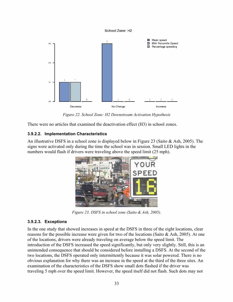
33

Figure 22. School Zone: H2 Downstream Activation Hypothesis

There were no articles that examined the deactivation effect (H3) in school zones.

3.9.2.2. Implementation Characteristics

An illustrative DSFS in a school zone is displayed below in Figure 23 (Saito & Ash, 2005). The signs were activated only during the time the school was in session. Small LED lights in the numbers would flash if drivers were traveling above the speed limit (25 mph).

Figure 23. DSFS in school zone (Saito & Ash, 2005).

3.9.2.3. Exceptions

In the one study that showed increases in speed at the DSFS in three of the eight locations, clear reasons for the possible increase were given for two of the locations (Saito & Ash, 2005). At one of the locations, drivers were already traveling on average below the speed limit. The introduction of the DSFS increased the speed significantly, but only very slightly. Still, this is an unintended consequence that should be considered before installing a DSFS. At the second of the two locations, the DSFS operated only intermittently because it was solar powered. There is no obvious explanation for why there was an increase in the speed at the third of the three sites. An examination of the characteristics of the DSFS show small dots flashed if the driver was traveling 5 mph over the speed limit. However, the speed itself did not flash. Such dots may not

34

be effective as an indication that the driver is above the speed limit. Across the four measurement periods during the day, the increase was 1.2 mph.

3.9.3. Transition Zone The following articles focused in part or in whole on transition zones.

1. Cruzado & Donnell, 2009

2. Hallmark, et al., 2007

3. Hallmark & Hawkins, 2015

4. Hallmark et al., 2013

5. Kamyab et al., 2002

6. Schoenecker et al., n.d.

7. Ullman & Rose, 2005

8. Williamson & Fries, 2015

The particular hypotheses and significant findings for each of the studies on school zones are in Table A2 in Appendix A in Volume II.

3.9.3.1. Vote Count

Of the 29 sites where the change in the mean speed was measured at the DSFS in transition zones, all reported a significant reduction in speed. The 11 analyses of the 85th percentile speed at the DSFS reported a significant reduction. All three analyses of the percentage of travelers over the speed limit reported a significant reduction.

Figure 24. Transition Zone: H1 activation hypothesis

35

There were too few studies of the effect of the DSFS on the reduction in speed downstream of the DSFS to draw general conclusions regarding transition zones. With respect to the mean speed, the studies were split, one indicating a reduction (Williamson & Fries, 2015), one no change . With respect to the 85th percentile speed, the one analysis available found significant increase in the speed downstream of the DSFS. Finally, with respect to the percentage of travelers over the speed limit, the one analysis reported a reduction (Kamyab et al, 2002).

Figure 25. Transition Zone: H2 Downstream Activation hypothesis

There were no analyses of the deactivation effect (H3) in transition zones.

3.9.3.2. Implementation Characteristics

An example implementation of DSFS in a transition zone is given below in Figure 26. In this study, dynamic feedback speed signs were installed at 12 sites in rural Pennsylvania (Cruzado & Donnell, 2009). The sites included both curved and straight sections of roadway where a transition was being made from a two-lane highway to a rural community. The posted speed limits of the highway upstream of the transition zone were 45 mph to 55 mph. The posted speed limits in the transition zone were 25 mph to 35 mph. Figure 26 shows the distance of the speed limit signs to the DSFS (labeled DSDS in the figure) and the location of the sensors and their distance from the DSFS. Often this information needed to be determined from a description written purely in text that could be difficult to piece together.

36

Figure 26. Data collection site setup. (SL = speed limit sign). (Cruzado & Donnell, 2009)

3.9.3.3. Exceptions

All analyses that reported a change in the mean speed at the DSFS when the DSFS was activated indicated a significant reduction.

3.9.4. Curved Section The following articles focused in part or in whole on curved sections of roadways (see reference section).

1. Bertini et al., 2006)

2. Bullough et al., 2012

3. Drakopoulos & Uprety, 2003

4. Hallmark et al., 2015

5. Knapp & Robinson, 2012

6. Tribbett et al., 2000

7. Ullman & Rose, 2005

8. Western Transportation Institute, 2003

The particular hypotheses and significant findings for each of the studies on curved sections are in Table A4, Appendix A of Volume II. Vote count. Thirty-four analyses were undertaken of the change in the mean speed at the DSFS after the DSFS was activated on curved sections of roadways. Of these, there was a significant reduction in the mean speed in 29 analyses, and similarly 27 sites showed decreases in the 85th

37

percentile speed. There were many fewer analyses of the change in the percentage of drivers exceeding the speed limit. All three the analyses indicated a reduction in this percentage.

Figure 27. Horizontal Curve: H1 Activation hypothesis

Relatively speaking, there was less support for a decrease in speed downstream of the DSFS after it was activated, 10 analyses showing decreases and five showing no change (Tribbett, McGowen, & Mounce, 2000). The three analyses of the 85th percentile speed and the percentage of drivers traveling over the speed limit showed decreases.

Figure 28. Horizontal Curves: H2 Downstream Activation hypothesis

There were no analyses of the effect of deactivating the DSFS on the speed at the DSFS (H3).

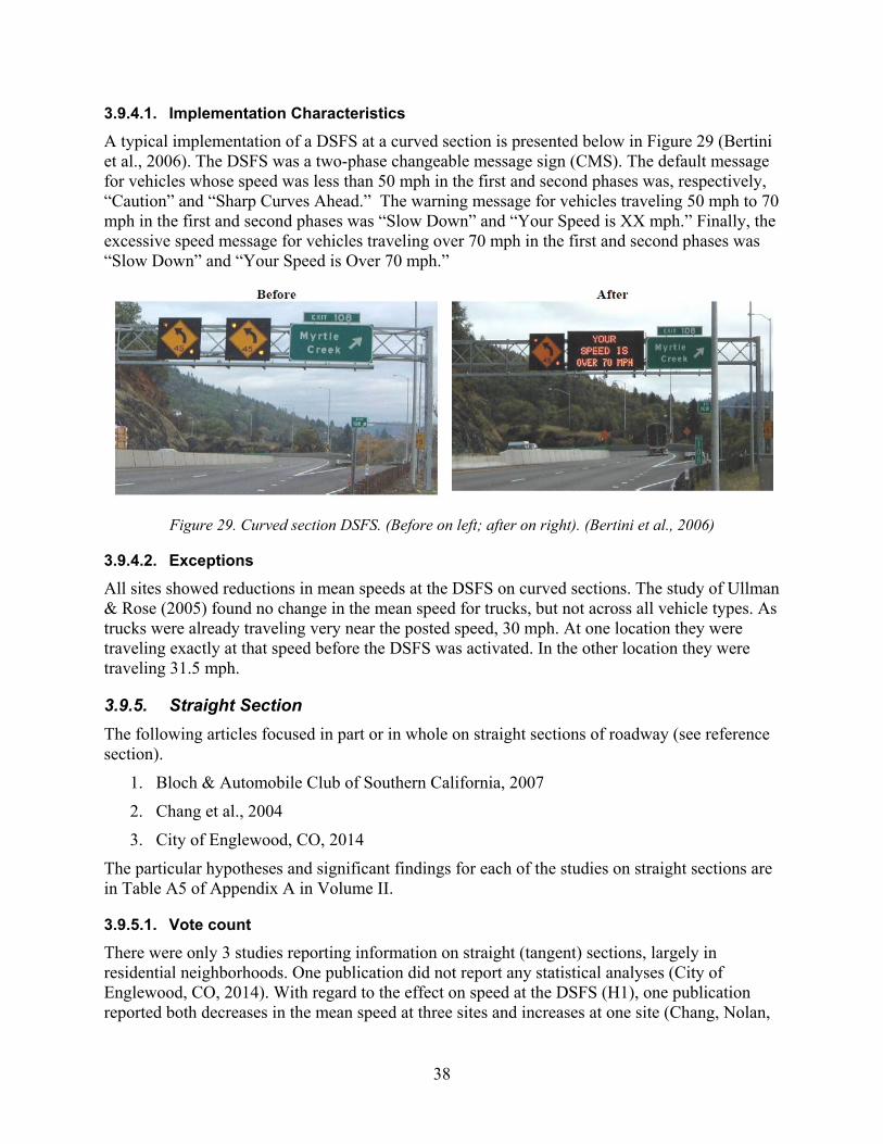
38

3.9.4.1. Implementation Characteristics

A typical implementation of a DSFS at a curved section is presented below in Figure 29 (Bertini et al., 2006). The DSFS was a two-phase changeable message sign (CMS). The default message for vehicles whose speed was less than 50 mph in the first and second phases was, respectively, “Caution” and “Sharp Curves Ahead.” The warning message for vehicles traveling 50 mph to 70 mph in the first and second phases was “Slow Down” and “Your Speed is XX mph.” Finally, the excessive speed message for vehicles traveling over 70 mph in the first and second phases was “Slow Down” and “Your Speed is Over 70 mph.”

Figure 29. Curved section DSFS. (Before on left; after on right). (Bertini et al., 2006)

3.9.4.2. Exceptions

All sites showed reductions in mean speeds at the DSFS on curved sections. The study of Ullman & Rose (2005) found no change in the mean speed for trucks, but not across all vehicle types. As trucks were already traveling very near the posted speed, 30 mph. At one location they were traveling exactly at that speed before the DSFS was activated. In the other location they were traveling 31.5 mph.

3.9.5. Straight Section The following articles focused in part or in whole on straight sections of roadway (see reference section).

1. Bloch & Automobile Club of Southern California, 2007

2. Chang et al., 2004

3. City of Englewood, CO, 2014

The particular hypotheses and significant findings for each of the studies on straight sections are in Table A5 of Appendix A in Volume II.

3.9.5.1. Vote count

There were only 3 studies reporting information on straight (tangent) sections, largely in residential neighborhoods. One publication did not report any statistical analyses (City of Englewood, CO, 2014). With regard to the effect on speed at the DSFS (H1), one publication reported both decreases in the mean speed at three sites and increases at one site (Chang, Nolan,

39

& Nihan, 2004). The third publication (Bloch & Automobile Club of Southern California, 2007) reported statistically significant reductions in 85th percentile speeds along straight sections for all 31 sites examined.

Figure 30. Straight Section: H1 Activation hypothesis

With regard to the effect of the activation of the DSFS on speed downstream of the DSFS (H2) or the halo effect of deactivation of the DSFS, no statistically significant results were reported.

3.9.5.2. Implementation Characteristics

A typical layout for a DSFS on a residential street is displayed below in Figure 31 (Chang et al., 2004). The DSFS is located directly below the speed limit sign.

Figure 31. Chang, Nolan, and Nihan (2004)

40

3.9.5.3. Exceptions

No studies indicated failure to produce a decrease in speed at the DSFS when it was activated (H1). Given that, we went on to look at possible exceptions to H2. One study found an increase in the speed downstream of the DSFS after it was activated (Chang et al., 2004). Again, we asked why this might have occurred. The authors speculate that it is the fact that this location already had lower speeds: “Because of this sign’s close proximity to Helen Keller Elementary School, this location had the lowest average speed of the four locations before installation. It can be speculated that drivers were already respecting the rules of the road, and this suggests that these signs may be better suited for locations with higher average speeds from the outset.” However, another explanation is possible. It appears that there is an outlier in the before data in the month of April. The speeds in the 3 months prior to the activation of the DSFS were 21.9 (April 2001), 27.6 (February 2002), and 27.0 mph (June 2002). The speeds in the 4 months during activation were 26.3 (June 2002), 25.9 (August 2002), 26.2 (January 2003), and 25.4 mph (April 2004). The authors did not explore the reason for this possible outlier.

3.10. Discussion Strong support for the effectiveness of DSFS was found when a vote count is used as the basis for support. Signs reduce the mean speed, the 85th percentile speed and the percentage of drivers traveling above the speed limit at the DSFS (H1, Figure 15), and downstream of the DSFS in large numbers (H2, Figure 16). There are indications of a significant halo effect after the DSFS is deactivated, although the sample size is limited to 3 studies (H3).

The support for the downstream hypothesis is substantial, although less overwhelming than support for the activation hypothesis. Fully 92 percent of the analyses show a significant reduction in speed at the DSFS whereas 68 percent of the analyses show a significant reduction in speed downstream of the DSFS. Importantly, this support is equally strong both adjacent to and downstream of the DSFS for reductions in the 85th percentile speed and reductions in the percentage of drivers traveling over the speed limit (Table 3).

3.10.1. Safety Focus We identified five primary safety focal points: work zones, school zones, transition zones, curved sections and straight sections. There was a clear variation in the effectiveness of the DSFS on the reduction in speed at the DSFS (H1), with the smallest proportion of studies showing an effect (80%) in school zones and the most in transition zones (100%, Table 3).

The finding that only 80 percent of studies showed significant effects in school zones results partly from the sample size of studies, and particular design features of the studies showing no significant effect. Fifteen studies looked at the effect of the DSFS at school zones, of which 3 reported negative results, all from the same publication (Saito & Ash, 2005). However, 2 of these negative results were easily explained. In one case, vehicles were already traveling at the posted speed limit. In the other case, the signs were not functioning consistently across days given that they were solar powered. In the third case, the speed did not flash if drivers were traveling above the posted speed limit. Instead lights flashed above either side of the posted speed limit. Regardless, as was noted above, the change in speed, although not reduced with the DSFS in, was minimal.

41

More generally, three factors appeared to reduce the effect of the DSFS on the speed of vehicles. First, it would appear that a DSFS will be less effective at reducing the speeds of trucks than of automobiles. However, this is because the trucks are already traveling at the posted speed limits, thus there is little reason to reduce speed (Ullman & Rose, 2005). Second, it was noticed that a DSFS was less effective if the geometry of the roadway moved the potential for conflict further away from the drivers. So, for example, in one case, a work zone, the travel lane was separated from the workers by a buffer lane (Gambatese & Zhang, 2014). Drivers may well have felt that there was a safe margin separating them from the workers and therefore believed that there was less of a need to reduce their speed. Finally, if drivers of whatever vehicle, not just trucks, were already traveling at the posted speed limits, the DSFS was not likely to reduce the speed of the drivers (Saito & Ash, 2005). In fact, it could increase it, though still keeping it within the posted speed limits.

3.10.2. Limitations The primary limitation of this review is that many studies did not control for the fact that the observations were taken at different locations or at different times, and thus did not clearly state if they were testing activation, downstream, or deactivation hypotheses. Observations taken at the same location at different times might simply reflect changes across time, not changes introduced by the DSFS. Observations taken at the same time, but across different locations, might simply reflect changes in location, not changes introduced by the DSFS. Thus, many of the studies have results that may be affected by changes in time or location. In this literature review, we point out that there are 13 ways to answer the seemingly straightforward question, does a DSFS have an effect on speed. However, we find that the analyses that control for both confounding factors, report effect sizes that are similar (though not identical) to analyses that do not control for space or time. We hope that in the future, researchers can refer to this report to identify the precise hypotheses they are hoping to test and, ideally, take measures that allow a normalized hypothesis to be evaluated.

The second limitation of this study is that we could not provide an analysis of the effect of the details of the implementation that are most critical to producing the largest reductions in speed. This is primarily a consequence of the studies not reporting what a priori seem critical details, say, how far an upstream posted speed limit is from the DSFS. Without this information, it is not possible to recommend whether the DSFS should be placed, say 600 feet from the last posted speed limit, or say half a mile from the last posted speed limit. If researchers referred to a standard list of study design elements, both those that discussed the details of the DSFS implementation and those that discussed the details of the experimental design, not only would this improve the understanding of the characteristics that influence the effectiveness of a DSFS in a particular study, but it would allow for a meta-analysis aggregating results across studies in order to arrive at a much more general statement as to the effectiveness of the DSFS.

Ultimately, what is most encouraging is that, despite the large variation in so many of the critical details that define each study, the results overall, as measured by a vote count (this section), clearly support the use of DSFS to reduce traffic speeds. The meta-analysis (Section 4, below) informs which of these various details are the most likely to impact the various functions of speed for each of the three different ways of evaluating the effect of a dynamic speed feedback sign.

42

4. Meta-Analysis

4.1. Meta-Analysis Summary Each publication from the literature review that measured the effectiveness of DSFS was assessed for availability of the underlying data on vehicle speeds. These data were compiled, along with accompanying data on the location and timing of the speed measurements, vehicle type, safety focus, and any other relevant data. The compiled database was then used to carry out a statistical analysis across all the published studies, a meta-analysis, to estimate the size of the speed reduction effects.

For each of the three major hypotheses, the activation hypothesis, downstream hypothesis, and deactivation hypothesis, reductions in speed were observed when the speeds at the DSFS and downstream of the DSFS were compared with the speeds upstream of the DSFS before activation (H1C, H2C, H3C, Table 5). Although the reductions in speed were observed, these reductions were statistically significant only for the activation hypothesis (Table 8).

For the three variations of the activation hypothesis (Volume I, Section 1.7) the size of the estimated reduction ranged from 2 to 4 mph depending on the actual hypothesis being evaluated (Table 6, Table 7, Table 8), with the largest estimated reduction obtained when the speeds of passenger cars at the DSFS before and during activation were observed (4.14 mph reduction, Figure 3, Table 7). All such reductions were statistically significant.

Safety focal points, surprisingly, did not show consistent differences in the size of the estimated speed reduction. There were only enough observations to compare the different estimates of the size of the estimated speed reduction across safety focal points for studies that evaluated the activation hypothesis using normalized estimates. The smallest speed reduction within a safety focus was for horizontal curves (2.27 mph) and the largest for school zones (3.21 mph, Table 6).

The speed differences in response to DSFS for passenger cars and trucks showed a consistent trend, with trucks less responsive to DSFS than passenger cars. Passenger cars slowed down by approximately 4 mph at the DSFS when it was active, with effects persisting downstream and to some extent even after signs were removed. Trucks exhibited smaller speed reductions in response to DSFS installations. As trucks are traveling more slowly than passenger cars on average, DSFS have smaller effects on their vehicle speed.

Overall, these results indicate that DSFS installations were consistently effective in reducing driver speeds at the DSFS. Speeds also decreased downstream of DSFS installations when measured with respect to the upstream speeds. Following removal of the DSFS, the few studies available indicated that vehicle speeds at the former site of the DSFS remained lower than the speeds were prior to the installation, giving evidence for a “halo effect.” As noted earlier, reductions in speed of even a few miles per hour can be of large practical significance when it comes to reducing the frequency of severe injuries and fatalities (Kloeden et al., 1997). For example, at relatively low speeds the risk of severe injury to pedestrians decreases from 50 percent to 25 percent as the speed at impact decreases from 31 mph to 23 mph (Tefft, 2011). Therefore, the reductions observed here as a result of DSFS installation would be expected to have a substantial effect on public safety.

43

4.2. Introduction

Following the literature review, it was clear that a sufficient number of publications were available in the literature to carry out a statistical analysis of DSFS effectiveness. While the literature review provided encouraging results about the effectiveness of DSFS installations, it cannot be determined from a simple count whether the results across all studies within a given safety focus are statistically significant. Nor can it be determined how large a reduction in speed is observed and whether that reduction is not only statistically, but also practically significant. The purpose of this research is to conduct a meta-analysis of the studies described above for each of the five safety focal points and for both heavy and light duty vehicles.

The direct and indirect advantages of such a meta-analysis are threefold. First, a meta-analysis allows one to draw general conclusions about the overall statistical significance of an intervention that has been evaluated in several studies, some of which are consistent with the hypothesis one is evaluating and some of which are not (the case with DSFS). Second, a meta-analysis allows one to compute appropriately weighted estimated effect sizes so that one can determine the practical significance of any given effect in different contexts. Specifically, one can estimate the reduction in speed attributable to the installation of a DSFS and then use appropriate tables (or formulas) to map this reduction in speed to a reduction in pedestrian-vehicle injuries and fatalities. Third, in performing a meta-analysis one needs to be very careful to make sure when one is combining studies that the studies are all evaluating the same hypothesis. The last point is especially relevant for DSFS effectiveness studies, as there is not a single hypothesis being tested to evaluate the effect of a DSFS, but rather 13 different hypotheses, as explained in Section 3.4. In addition to contributing to what is known about the effect of a DSFS in different contexts and with different vehicle types, this study provides a novel conceptual framework for identifying and categorizing the 13 different hypotheses. This conceptual framework facilitates the comparison between and among studies, as the hypotheses being evaluated in previous comparisons have typically been unidentified.

To carry out the meta-analysis, publications were reviewed for availability of the underlying data on vehicle speeds, in tabular or graphical form, and data were compiled in a database. The data were then analyzed using a meta-analysis. Meta-analysis is a statistical technique used to draw general conclusions from a set of related studies focused on similar experimental treatments and responses (Glass, 1976). Given sufficiently similar study designs, the sizes of the treatment effects can be pooled to create a meta-data set, which is then analyzed with appropriate weighting based on the variability and number of observations in each study. This meta-analysis aims to provide decision-makers with a quantitative estimate of how much vehicle speed is reduced following installation of a DSFS. Factors such as location, timing, vehicle type, posted speed, safety focus, and others are all considered in the meta-analysis model.

44

4.3. Methods

4.3.1. Data collection

Literature review publications (above) were assessed for availability of the underlying data on vehicle speeds. Data were entered at two levels.

(a) The descriptor level, which describes the characteristics of each study (the features that identify how the DSFS was implemented, the hypotheses that were evaluated, and the experimental design)

(b) The data level, which was the least-aggregated level of data reported either in tabular or graphical format in the publication. For calculations of effect size, at a minimum, a study would have to report the mean and standard deviation (SD) of vehicle speeds, as well as the number of vehicles observed, at either two points in time or two locations. The difference in whether studies focused on different timing or location of vehicle speed data collection determines that hypotheses can be tested (Section 3.4).

Publications in some cases included more than one study, meaning they tested DSFS with different safety focal points or in combinations with additional treatments such as police cruisers or speed radar enforcement; these are treated as separate studies in the data collection, grouped under the same publication ID. Studies could also include different sites (locations). Publications employed many different combinations of descriptors in the study design (and sometimes at the different sites within a study), and an effort was made to enter data from any relevant descriptor that could be expected to appear in several studies. Key descriptors, including posted speed, safety focus, vehicle type, sign type, and distance from sign the vehicle speeds, were measured.

4.3.2. Calculating Effect Size

Historically, meta-analyses were initially used primarily to assess the odds of a particular outcome, such as the odds a drug treatment would result in a favorable outcome for a patient, and then were expanded to more generally test the size and direction of the outcome across different studies. Both types of tests, assessing the odds of a categorical outcome or the size of a continuous outcome, are dependent on calculating the effect size. For the meta-analysis of DSFS, the outcomes are vehicle speeds at different points in time or at the same point in time and different locations. Three sets of hypotheses regarding the effectiveness of DSFS can be tested, and each requires a different calculation of effect size. These hypotheses are discussed in detail in the literature review (Section 3.4), and summarized here.

1. H1. Activation of the DSFS: adjacent. The extent to which the DSFS reduces driver speed at the DSFS (or immediately adjacent to the DSFS) is the central question for this analysis. The studies tested activation in three ways.

A. Compute a difference of differences: Compare the difference between the upstream and adjacent vehicle speeds before activation to the difference between the upstream and adjacent vehicle speeds during activation of the DSFS. This is the ideal comparison, or the true effect (Cruzado & Donnell 2009); we refer to it as the normalized version of H1;

45

B. Compare vehicle speeds adjacent to the DSFS before activation and then during activation; and

C. Compare vehicle speeds upstream (of the DSFS) and adjacent (to the DSFS).

2. H2. Activation of the DSFS: downstream. Safety officials may also consider installing a DSFS upstream of a zone of safety focus. For instance, well upstream of a transition zone between a rural highway and a settled area, it may be desired to begin tapering vehicle speeds. In this case, considering the downstream hypothesis (H2) would be appropriate. The downstream hypothesis is the same as the activation hypothesis except that it assesses the effectiveness of the DSFS on reducing vehicle speeds downstream of the DSFS, rather than adjacent to it. If the sign is placed too far upstream of the location of interest, vehicle speeds may recover to prior levels, so assessing the distance between the sign and the measurement location is critical. The studies tested the activation effect downstream in five ways.

A. (Normalize to upstream). Compute a difference of differences: Compare the difference between the speeds upstream of the DSFS (upstream) and speeds downstream of the DSFS (downstream) before activation with the difference between the upstream and downstream speeds after activation. This controls for variations in both the time at which the vehicle speeds (before and during activation) are measured and the location at which the vehicle speeds are measured (upstream and downstream of the DSFS);

B. Compare downstream vehicle speeds during activation to downstream vehicle speeds before activation;

C. Compare downstream vehicle speeds to upstream vehicle speeds during activation,

A’. (Normalize to adjacent). Compute a difference of differences: Compare the difference between the speeds adjacent to the DSFS (adjacent) and speeds downstream of the DSFS (downstream) before activation with the difference between the adjacent and downstream speeds after activation. This controls for variations in both the time at which the vehicle speeds (before and during activation) are measured and the location at which the vehicle speeds are measured (adjacent to the DSFS and downstream of the DSFS); and

C’. Compare downstream vehicle speed to adjacent speeds during activation.

Note that “H2B'” would compare vehicle speeds downstream of the DSFS during activation to vehicle speeds downstream of the DSFS before activation; this is identical to H2B, so is not listed as a separate hypothesis.

3. H3. Deactivation of the DSFS. Safety officials may consider temporarily installing a DSFS, for example as part of a mobile operation in a work zone or as a test case to evaluate DSFS effectiveness. Upon removal of the DSFS, it is possible that a halo effect of continued reductions in driver speed may be observed. Some authors have tested this deactivation hypothesis. As with the downstream hypothesis, there are five combinations of measurement in time and space that are possible. The first hypothesis (A) normalizes the adjacent speeds after deactivation to the upstream speeds before activation. The second (B) and third (C) hypotheses are subcomponents used in the calculation of A. The fourth hypothesis (A') normalizes the adjacent speeds after deactivation to the upstream speeds

46

during activation. The third (C) and fifth (B') hypotheses are subcomponents used in the calculation of A'.

A. (Normalize to before activation). Compute a difference of differences: Compare the difference between the speeds upstream of the DSFS (upstream) and speeds adjacent to the DSFS (adjacent) before activation with the difference between the upstream and adjacent speeds after deactivation.

B. Compare vehicle speeds adjacent to the DSFS before activation to vehicle speeds adjacent to the DSFS after deactivation.

C. Compare upstream vehicle speeds to adjacent vehicle speeds after deactivation.

A'. (Normalize to during activation). Compute a difference of differences: Compare the difference between the speeds upstream of the DSFS (upstream) and speeds adjacent to the DSFS (adjacent) during activation with the difference between the upstream and adjacent speeds after deactivation.

B'. Compare adjacent vehicle speeds during activation to adjacent vehicle speeds after deactivation.

We calculate the effect size (ES) associated with activation of the DSFS appropriately for each hypothesis. The calculation of effect sizes is based on, at minimum, measurements of speeds at two locations at the same time, or at two points in time at the same location. For the hypothesis H1B, for example, the effect size is based on the difference between the mean speeds adjacent to the DSFS during the period in which it is active, 𝑋𝑋𝐷𝐷𝐷𝐷𝑈𝑈𝐷𝐷𝐴𝐴𝐷𝐷𝐷𝐷𝐷𝐷𝐷𝐷𝐷𝐷 and the sample mean speed adjacent to the DSFS before activation 𝑋𝑋𝐵𝐵𝑈𝑈𝐵𝐵𝐷𝐷𝑈𝑈𝑈𝑈𝐷𝐷𝐷𝐷𝐷𝐷𝐷𝐷.

The ES is this difference, placed relative to units of the pooled standard deviation. The value is negative if there is a reduction in speed at the site of the DSFS installation.

𝐸𝐸𝐸𝐸 =𝑋𝑋𝐷𝐷𝐷𝐷𝑈𝑈𝐷𝐷𝐴𝐴𝐷𝐷𝐷𝐷𝐷𝐷𝐷𝐷𝐷𝐷 − 𝑋𝑋𝐵𝐵𝑈𝑈𝐵𝐵𝐷𝐷𝑈𝑈𝑈𝑈𝐷𝐷𝐷𝐷𝐷𝐷𝐷𝐷

𝐸𝐸𝐷𝐷𝑃𝑃𝐷𝐷𝐷𝐷𝑃𝑃𝑈𝑈𝐴𝐴 ,

where the pooled standard deviation for this calculation is defined as follows.

𝐸𝐸𝐷𝐷𝑃𝑃𝐷𝐷𝐷𝐷𝑃𝑃𝑈𝑈𝐴𝐴 = �(𝑁𝑁𝐷𝐷𝐷𝐷𝐷𝐷𝐷𝐷𝐷𝐷𝐷𝐷𝐷𝐷𝐷𝐷𝐷𝐷𝐷𝐷−1)𝐷𝐷𝐷𝐷𝐷𝐷𝐷𝐷𝐷𝐷𝐷𝐷𝐷𝐷𝐷𝐷𝐷𝐷𝐷𝐷𝐷𝐷𝐷𝐷𝑁𝑁𝐷𝐷𝐷𝐷𝐷𝐷𝐷𝐷𝐷𝐷𝐷𝐷𝐷𝐷𝐷𝐷𝐷𝐷𝐷𝐷+𝑁𝑁𝐵𝐵𝐵𝐵𝐵𝐵𝐵𝐵𝐷𝐷𝐵𝐵𝐷𝐷𝐷𝐷𝐷𝐷𝐷𝐷−2

+ (𝑁𝑁𝐵𝐵𝐵𝐵𝐵𝐵𝐵𝐵𝐷𝐷𝐵𝐵𝐷𝐷𝐷𝐷𝐷𝐷𝐷𝐷−1)𝐷𝐷𝐷𝐷𝐵𝐵𝐵𝐵𝐵𝐵𝐵𝐵𝐷𝐷𝐵𝐵𝐷𝐷𝐷𝐷𝐷𝐷𝐷𝐷𝑁𝑁𝐷𝐷𝐷𝐷𝐷𝐷𝐷𝐷𝐷𝐷𝐷𝐷𝐷𝐷𝐷𝐷𝐷𝐷𝐷𝐷+𝑁𝑁𝐵𝐵𝐵𝐵𝐵𝐵𝐵𝐵𝐷𝐷𝐵𝐵𝐷𝐷𝐷𝐷𝐷𝐷𝐷𝐷−2

.

This effect size calculation is also referred to as the standardized mean difference (SMD) (Hedges & Olkin, 1985).

For other hypotheses based on the comparison of two groups, such as comparing the effect of DSFS at two locations, adjacent to the DSFS and upstream of the DSFS (hypothesis H1A), the effect size calculation is similar. These normalized ES require a slightly modified calculation, where differences in means rather than means themselves are compared. For example, when the activation effect of the DSFS on vehicle speed is normalized for differences during and before installation, at both the site adjacent to the sign and upstream of the sign, the effect size is calculated on the next page.

47

𝐸𝐸𝐸𝐸 =(𝑋𝑋𝐷𝐷𝐷𝐷𝑈𝑈𝐷𝐷𝐴𝐴𝐷𝐷𝐷𝐷𝐷𝐷𝐷𝐷𝐷𝐷 − 𝑋𝑋𝐵𝐵𝑈𝑈𝐵𝐵𝐷𝐷𝑈𝑈𝑈𝑈𝐷𝐷𝐷𝐷𝐷𝐷𝐷𝐷) − (𝑋𝑋𝐷𝐷𝐷𝐷𝑈𝑈𝐷𝐷𝐴𝐴𝐷𝐷𝑈𝑈𝑈𝑈𝑈𝑈𝑈𝑈𝑈𝑈𝑈𝑈𝑈𝑈𝑈𝑈 − 𝑋𝑋𝐵𝐵𝑈𝑈𝐵𝐵𝐷𝐷𝑈𝑈𝑈𝑈𝑈𝑈𝑈𝑈𝑈𝑈𝑈𝑈𝑈𝑈𝑈𝑈𝑈𝑈𝑈𝑈)

𝐸𝐸𝐷𝐷𝑃𝑃𝐷𝐷𝐷𝐷𝑃𝑃𝑈𝑈𝐴𝐴 .

The pooled standard deviation in this case is computed as follows.

𝐸𝐸𝐷𝐷𝑃𝑃𝐷𝐷𝐷𝐷𝑃𝑃𝑈𝑈𝐴𝐴 = �(𝑁𝑁1 − 1)𝐸𝐸𝐷𝐷1 + (𝑁𝑁2 − 1)𝐸𝐸𝐷𝐷2 + (𝑁𝑁3 − 1)𝐸𝐸𝐷𝐷3 + (𝑁𝑁4 − 1)𝐸𝐸𝐷𝐷4

𝑁𝑁1 + 𝑁𝑁2 + 𝑁𝑁3 + 𝑁𝑁4 − 4 .

The subscripts on each variable identify the relevant time and location at which the variable is measured: 1. Adjacent to the DSFS, during activation; 2. Adjacent to the DSFS location but before activation; 3. Upstream of the DSFS during activation; and 4. Upstream of the DSFS location, but before activation. Figure 12, Figure 13, and Figure 14 in the literature review provide the detailed speed reduction formulas for each of the 13 possible combinations of timing and location of vehicle speeds in response to DSFS installation. The specific calculations follow the two forms above, for either the direct or normalized measurement of effect size.

4.3.3. Hypothesis testing This meta-analysis investigates a single continuous outcome (speed of vehicles) across several studies, with both fixed effects, two moderating variables (posted speed, distance from DSFS at which the speed is measured) and random effects. The random effects are safety focal points (five levels) and vehicle classes (two levels), and studies within publications. The use of several moderating and independent variables along with fixed and random effects in a meta-analysis has also been called meta-regression (van Houwelingen et al., 2002). This type of analysis is best conducted using a mixed-effect model, where the intercepts for the publications and for the studies within publications are the random effects and the moderating and independent variables are the fixed effects. "Random effects" refers to variables in the model that are assumed to be representatives of a larger population (Raudenbush, 2009; Hedges & Vevea, 1998), and are useful as grouping variables when sample sizes are unbalanced between groups.

When possible, the full model was employed as follows. 𝑦𝑦𝐷𝐷 = 𝛽𝛽0 + 𝛽𝛽1𝑝𝑝𝐵𝐵𝑝𝑝𝐴𝐴𝐵𝐵𝑝𝑝. 𝑝𝑝𝑝𝑝𝐵𝐵𝐵𝐵𝑝𝑝𝐷𝐷 + 𝛽𝛽2𝑝𝑝𝐷𝐷𝑝𝑝𝐴𝐴𝑖𝑖𝐷𝐷𝑖𝑖𝐵𝐵. 𝐵𝐵𝐷𝐷𝐵𝐵𝑓𝑓. 𝑝𝑝𝐷𝐷𝐷𝐷𝐷𝐷𝐷𝐷 + 𝑈𝑈𝐷𝐷 + 𝐵𝐵𝐷𝐷

where i indexes the site. 𝛽𝛽0 refers to the overall intercept, while the terms 𝛽𝛽1 and 𝛽𝛽2 refer to the coefficients for each of the predictor variables. Each hypothesis did not always include the moderator variables. When no information was available, the moderator variable was dropped from the analysis for the evaluation of a given hypothesis. Where some information was available and an estimate could be made of the moderator variable, it was included in the analysis. As for random effects, at a minimum the statistical analysis always included a term for study, nested within publication ID. In many cases the posted speed and distance from sign values were not available, thus this report focuses on overall speed reduction effect sizes.

The error term has several parts. The first term 𝑈𝑈𝐷𝐷 represents the random effects, which for this model include the effect of study, nested within publication, as well as safety focus and vehicle type. For example, the study-level error term 𝐷𝐷𝐷𝐷 is defined as 𝐷𝐷𝐷𝐷 ∼ 𝑁𝑁(0, 𝜏𝜏2), a normally distributed error term with a mean of zero and variance 𝜏𝜏2; this variance is estimated in the model. As a random effect, it represents the variability assumed from the larger population of

48

studies within publication ID from which the specific studies used have been drawn. The random effects allow the model to fit unbalanced data, which is the case for all of the hypotheses tested, and to account for the hierarchical nature of the data, with several studies being conducted in some publications. This mixed effect approach (mixing random and fixed effects) allows estimates for how the different levels of the random effects contribute to the overall effect, for instance how passenger cars differ from commercial motor vehicles in their response to DSFS installations.

The remaining error term 𝐵𝐵𝐷𝐷 is defined as 𝐵𝐵𝐷𝐷 ∼ 𝑁𝑁(0, 𝑣𝑣𝐷𝐷), meaning that the residual error is normally distributed with a mean of zero and a standard deviation of 𝑣𝑣𝐷𝐷; this standard deviation 𝑣𝑣𝐷𝐷 is directly computed in the effect size calculation. The quantity 𝑣𝑣𝐷𝐷 becomes important in the model fitting process, giving greater weight to studies that have a lower variability in the response, due to a large sample size, a low standard deviation in the speeds, or a combination of the two.

For each of the 13 hypotheses tested, a similar structure of models was used. Establishing which fixed and random effect variables could be used depended on data availability. At a minimum, the statistical analysis always included a term for study, nested within publication ID. Safety focus and vehicle type were included as random effects in nearly all models. Posted speed and distance from DSFS (fixed effects) were available for only a subset of the hypothesis tests.

This analysis allows results to be presented on the overall effectiveness of DSFS in reducing speeds for a particular hypothesis, for example the overall effect of DSFS activation when comparing speeds measured at the DSFS sign during activation of the DSFS to speeds measured at the site of the DSFS sign prior to sign installation (hypothesis H1B). In addition to this overall measure of speed reduction, this analysis will further allow reporting of how much the posted speed drives the speed reduction, how much the speed reduction differs for passenger cars versus commercial vehicles, and how much the speed reduction differs for school zones, work zones, rural-to-urban transition zones, or other safety focus areas. The combination of several hypotheses tested and several moderating variables should assist traffic safety practitioners in determining where and when to deploy DSFS for maximum effect, and the size of the speed reduction they can expect to observe.

All of the effect size calculations and calculations of sample standard deviation were carried out in the meta-analysis package metafor (Viechtbauer, 2010) using the statistical programming language R (R Core Team, 2016). In R, the model is written as follows.

Effect.size ~ posted.speed + distance.from.sign + (1|safety.focus) + (1|vehicle.type) + (1|PublicationID/StudyID)

The term (1| safety.focus) means that there is a random effect for safety focus site. The term (1|PublicationID/StudyID) means that a lower level factor, in this case StudyID, appears only within a particular level of an upper level factor, in this case PublicationID. Functions for calculating normalized effect sizes (e.g., H1A) were written using the metafor functions as a foundation. Hypothesis testing was carried out using the linear mixed-effect model package lme4 (Bates et al., 2015). The effect size calculations in metafor have been validated against results provided by the software packages Stata, SAS, and SPSS; the results from these other packages either agreed completely or fell within a margin of error expected when using numerical

49

methods. The results of metafor effect size calculations and analyses have also been validated against textbook examples.

4.4. Results

4.4.1. Summary of data

The literature review identified 43 publications with data appropriate for a quantitative meta-analysis. From these publications, 57 studies were included, with 204 sites at which the effectiveness of DSFS was evaluated (Table 4). By assessing the availability of the appropriate data (mean, SD, and N) within sites at the appropriate locations, the number of publications, studies, and sites available for testing each hypothesis can be calculated. This shows that hypothesis H1, the effect of DSFS activation at the site of the sign, is the most commonly studied design, followed by H2, the effect of DSFS activation downstream of the sign. Hypothesis H3, the effect of DSFS following deactivation of the sign, was rarely studied, with only three publications providing sufficient data for a meta-analysis. Note that these values differ from the literature review vote count analysis, which only required for inclusion in the vote count that studies report the significance of the result, not necessarily that the studies report the underlying data for a meta-analysis.

Table 4. Summary of the number of publications, studies, and individual sites with data for each the 13 hypotheses.

Hypothesis Publications Studies Sites H1A 12 22 81 H1B 18 36 186 H1C 14 28 123 H2A 9 18 85 H2B 9 18 85 H2C 9 18 85 H2A' 9 18 85 H2C' 9 18 85 H3A 2 3 8 H3B 3 5 8 H3C 2 3 4 H3A' 2 3 4 H3B' 3 5 8

The actual number of sample units available for each hypothesis test was greater than the number of sites in some cases, if studies separately investigated different vehicle types, for example. If some sites had insufficient data to carry out the statistical test (for example, lacking standard deviations reported), then the number of sample units was less than the number of sites in some cases. The mean difference in speeds (MD), variance (Var), and number of sample units (N) for each of the thirteen hypotheses are presented in Table 5. To be clear, these are not the changes in

50

speeds as estimated by the meta-analysis. Rather, these are the numerators of the effect size (ES) calculations referred to in Section 4.3.2. These numerators we refer to as MD.

The mean differences in speed are noted for decreases in speed due to activation of the sign, at the site of the DSFS (H1B, 2.99 mph decrease). For the downstream activation effects, the largest mean effect size was for the downstream effect calculated relative to speeds upstream of the DSFS (H2C, 6.98 mph decrease). As expected, when measured with respect to the speed at the DSFS during activation, the downstream speeds were faster (H2A', H2B'). Finally, deactivation effects were heterogeneous depending on what hypothesis was tested, but had high effect sizes for the reduction in speed between upstream and adjacent sites, following DSFS removal (H3C, 9.44 mph decrease). Again, as expected, when measured with respect to the speed at the DSFS during activation, there was an increase in speeds at the DSFS after deactivation (H3A', H3C').

Taken together, these results indicate that DSFS installations were consistently effective in reducing driver speeds at the DSFS, typically by 2 to 4 mph for passenger cars. Speeds generally increased downstream of DSFS installations when measured with respect to upstream speeds, indicating that the effect of the DSFS on driver behavior is not confined to just vehicles adjacent to the DSFS. Following removal of the DSFS, the few studies available indicated that vehicle speeds at the former site of the DSFS remained lower than prior to the installation when the speeds at the DSFS were measured with respect to the upstream speeds, giving evidence for a halo effect following removal of temporary DSFS installations.

A final caveat is in order. The mean differences in Table 5 are calculated at the level of a sample unit. The definition of a sample unit varies by hypothesis, and may include a single site measured at two points in time (e.g., H1B), two sites measured at the same time (H1C), or two sites, each measured at two points in time (H1A and other normalized effect sizes).

51

Table 5. Summary of mean difference in speeds (MD, in mph) across the 13 hypotheses tested, with variance (Var) and sample size (N) indicated. These values represent average effect sizes, without

accounting for publication-specific features. Statistical modeling of effect sizes follows below.

Hypothesis Category Hypothesis MD Var N H1: Activation H1A -2.73 1.88 72 H1B -2.99 0.89 249 H1C -2.73 2.00 49 H2: Downstream H2A -1.15 1.21 35 H2B -2.57 0.59 162 H2C -6.98 0.02 4 H2A' 2.65 1.06 67 H2C' 7.21 0.41 40 H3: Deactivation H3A -0.40 0.01 2 H3B -0.68 0.61 20 H3C -9.44 0.07 4 H3A' 2.60 0.01 2 H3B' 1.89 0.37 82

The sections below go beyond the above and employ statistical models to account for the differences between publications, studies within publications, vehicle types, and safety focal points. Further analysis was carried out, where possible, to address the effect on speed reductions both of the posted speed and of the distance between DSFS and measured speed.

4.4.2. H1: Activation hypothesis

As described in detail in Section 3.4, the three versions of the activation hypothesis H1 all rely on a measurement of vehicle speeds at the site of the DSFS, but use different baseline comparisons. The simplest, H1B, compares vehicle speeds at the site of the sign between the time before activation and during activation. H1A calculates a similar value, for the difference between activation timing (before and during), normalized to the same difference upstream of the DSFS. H1C compares speeds at the DSFS to speeds upstream, at the same time. Across all three activation hypothesis tests, statistically significant reductions in speed were observed.

4.4.2.1. H1A: Activation effect at DSFS, normalized relative to upstream

Overall, the decrease in speed attributed to DSFS, normalized by upstream location, is 2.84 mph, a significant effect (p = 0.004). For the vehicle type grouping variable, cars demonstrated a slowing effect 0.22 mph greater than that of trucks. Of the studies that specifically identified the safety focus, the largest reduction in the estimated speed was noted in school zones (-3.21 mph). When carrying out the statistical analysis of these effect sizes, 72 sites were available. Neither posted speed nor distance from sign location were significant predictors of the decrease in speed.

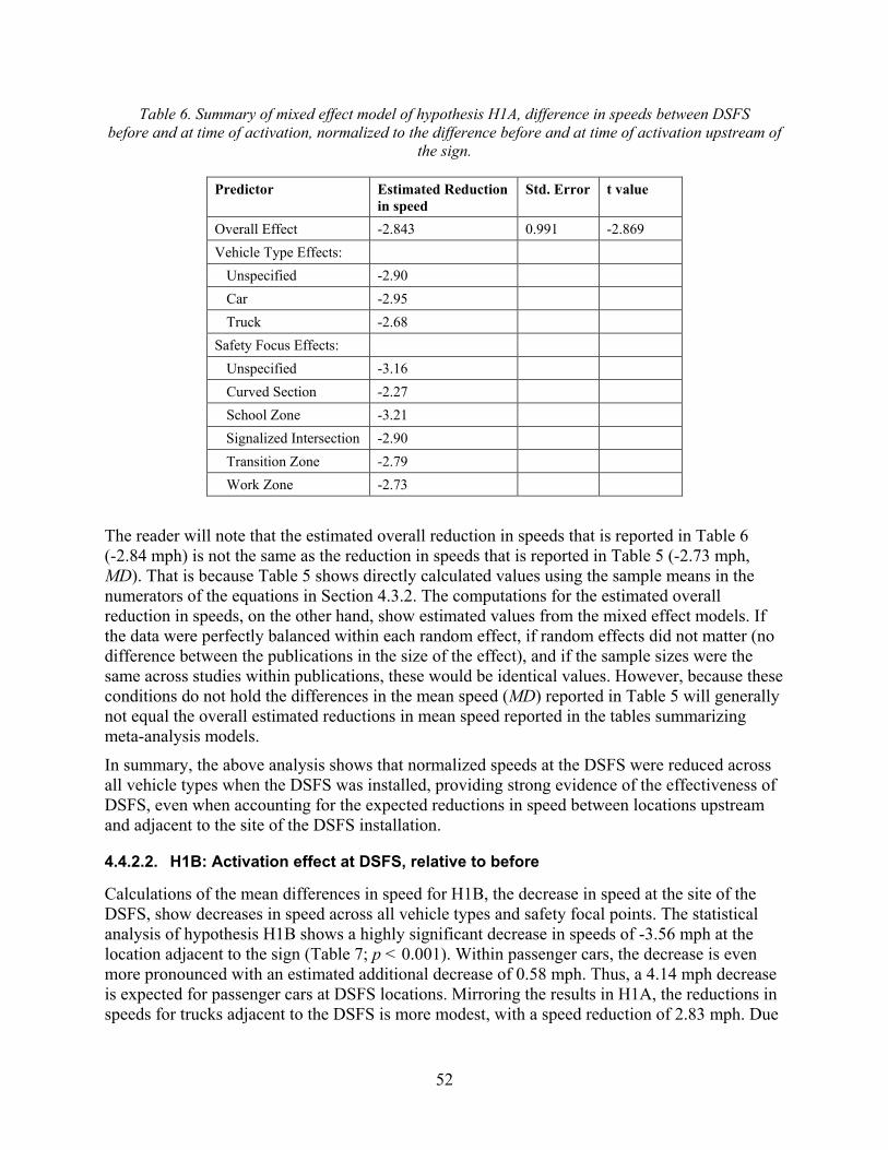
52

Table 6. Summary of mixed effect model of hypothesis H1A, difference in speeds between DSFS before and at time of activation, normalized to the difference before and at time of activation upstream of

the sign.

Predictor Estimated Reduction in speed

Std. Error t value

Overall Effect -2.843 0.991 -2.869 Vehicle Type Effects:

Unspecified -2.90 Car -2.95 Truck -2.68

Safety Focus Effects: Unspecified -3.16 Curved Section -2.27 School Zone -3.21 Signalized Intersection -2.90 Transition Zone -2.79 Work Zone -2.73

The reader will note that the estimated overall reduction in speeds that is reported in Table 6 (-2.84 mph) is not the same as the reduction in speeds that is reported in Table 5 (-2.73 mph, MD). That is because Table 5 shows directly calculated values using the sample means in the numerators of the equations in Section 4.3.2. The computations for the estimated overall reduction in speeds, on the other hand, show estimated values from the mixed effect models. If the data were perfectly balanced within each random effect, if random effects did not matter (no difference between the publications in the size of the effect), and if the sample sizes were the same across studies within publications, these would be identical values. However, because these conditions do not hold the differences in the mean speed (MD) reported in Table 5 will generally not equal the overall estimated reductions in mean speed reported in the tables summarizing meta-analysis models.

In summary, the above analysis shows that normalized speeds at the DSFS were reduced across all vehicle types when the DSFS was installed, providing strong evidence of the effectiveness of DSFS, even when accounting for the expected reductions in speed between locations upstream and adjacent to the site of the DSFS installation.

4.4.2.2. H1B: Activation effect at DSFS, relative to before

Calculations of the mean differences in speed for H1B, the decrease in speed at the site of the DSFS, show decreases in speed across all vehicle types and safety focal points. The statistical analysis of hypothesis H1B shows a highly significant decrease in speeds of -3.56 mph at the location adjacent to the sign (Table 7; p < 0.001). Within passenger cars, the decrease is even more pronounced with an estimated additional decrease of 0.58 mph. Thus, a 4.14 mph decrease is expected for passenger cars at DSFS locations. Mirroring the results in H1A, the reductions in speeds for trucks adjacent to the DSFS is more modest, with a speed reduction of 2.83 mph. Due

53

to the limited sample size, safety focus estimates were not able to be calculated; for further analyses where not all effects are reported, similar limitations on sample size apply.

Table 7. Summary of mixed effect model of hypothesis H1B, difference in speeds between DSFS before and at time of activation.

Modeled Effect Sizes Estimate Std. Error t value

Overall Effect -3.562 0.736 -4.843

Vehicle Type Effects:

Unspecified -3.72

Car -4.14

Truck -2.83

4.4.2.3. H1C: Activation effect at DSFS, relative to upstream

The difference between speeds upstream and adjacent to DSFS during activation of the DSFS (measured at the same time) were surprisingly large, with an overall -8.62 mph (Table 8) decrease estimated (p = 0.008). The largest decreases were detected in several studies that did not differentiate by vehicle type (Hallmark, et al., 2007; Reddy et al., 2008; Roberts & Smaglik, 2012). Due to the limited sample size, safety focus and vehicle type estimates could not be calculated. The large decrease in speeds from upstream to adjacent sites can be attributed in particular to the studies of Hallmark et al. (2007), who studied the effect of DSFS installations at transition zones in rural communities, Gambatese and Jafarnejad (2015), and Reddy et al. (2008), who studied the effects of DSFS installations in work zones. Transition zones and work zones are places where the posted speed several miles upstream of the DSFS is likely to be much greater than the posted speed closer to the DSFS. Whether they would have observed such large reductions had the normalized version of the activation hypothesis (H1A) been evaluated is open to question for the reasons discussed above. Table 8. Summary of mixed effect model of hypothesis H1C, difference in speeds between DSFS upstream

and adjacent to the sign.

Modeled Effect Sizes Estimate Std. Error t value Overall Effect -8.615 3.254 -2.647 Publication ID Effects:

Gambatese et al. (2015) -10.41 Hallmark et al. (2007) -15.60 Reddy et al. (2008) -13.60 Roberts et al. (2012) -2.96 Tribbett et al. (2000) -0.50

54

4.4.3. H2: Downstream Hypothesis

After drivers move past the DSFS installation, the extent to which speeds increase again is an important point to consider. Those speeds can be measured either with respect to the upstream DSFS or the adjacent DSFS. When the upstream speed was the baseline, a reduction in speed downstream of the DSFS was estimated to occur and, consistent with the previous analyses, the smallest estimated reduction was seen with the normalized measure (-0.94 mph, H2A, versus -5.44 mph, H2B). Note that there was not enough information to estimate this reduction for H2C. However, perhaps not surprisingly, when the adjacent speed was the baseline, an increase in speed downstream of the DSFS was measured. Again, the effect was more moderate when a normalized index was used (2.51 mph, H2A') than when a simple comparison was used (4.17 mph, H2C').

4.4.3.1. H2A: Downstream effect normalized, relative to upstream

As for the activation hypothesis, a normalized difference in speeds can be calculated to address the downstream effect. Similar to H1A, where the differences in speeds upstream of and adjacent to the DSFS were calculated normalized to the timing of DSFS activation, H2A calculates a difference between the upstream and downstream sites, normalized by the timing of activation.

The statistical analysis of this hypothesis shows a modest trend for speed to decrease, when normalized, of only 0.94 mph. The reduction was not statistically significant (p = 0.148). In this case, sufficient variation at the grouping level was only available for safety focus. Of the two safety focal points included where the studies identified the location, work zones showed a stronger decrease (-1.37 mph) than did curves (-0.78). This same order was observed in the test of H1A.

Table 9. Summary of mixed effect model of hypothesis H2A.

Modeled Effect Sizes Estimate Std. Error t value Overall Effect -0.942 0.652 -1.445 Safety Focus Effects: Unspecified -0.68 Horizontal curve -0.78 Work zone -1.37

4.4.3.2. H2B: Downstream effect, relative to before

There were decreases in the estimated speed downstream of the DSFS (measured before and during activation) across all vehicle types and locations. The statistical analysis of hypothesis H2B shows a large decrease in speeds of 5.44 mph downstream of DSFS installations, a trend however that was not statistically significant. (p = 0.099). This trend was quite similar across vehicle types, with only slightly larger decreases observed for passenger cars of 5.55 mph. Though slight, the direction of the changes is consistent with what was observed for passenger cars and trucks in the evaluation of the activation hypothesis. These large decreases should be interpreted with caution, as very large downstream differences were detected in Fontaine et al. (2001), which analyzed effects of DSFS installations in work zones in Texas.

55

Table 10. Summary of mixed effect model of hypothesis H2B, difference in speeds downstream of DSFS sites, before and at time of activation.

Modeled Effect Sizes Estimate Std. Error t value

Overall Effect -5.439 3.304 -1.646

Vehicle Type Effects:

Unspecified -5.44

Car -5.55

Truck -5.33

4.4.3.3. H2C: Downstream effect, relative to upstream

The downstream effect of DSFS can be further analyzed by focusing on just the time during the DSFS activation. Comparing speeds detected downstream of the DSFS to speeds upstream of the DSFS is the focus of hypothesis H2C. Here, an insufficient number of studies were conducted either to carry out a breakdown of DSFS effectiveness by vehicle type or safety focus, or to employ the full statistical model. However, the overall effect can be assessed using the mean differences. In this case a decrease of -6.98 mph was observed in the mean speeds (Table 5).

4.4.3.4. H2A': Downstream effect normalized, relative to adjacent

As with H2A, which normalized the difference by comparing upstream and downstream speeds, before and during DSFS activation, H2A' examines the adjacent and downstream speeds, both before and during DSFS activation. Compared to H2A, the difference is now that the reference level is adjacent to the DSFS; therefore, the relative speed difference may be expected to be a positive value, as vehicles accelerate following the DSFS.

Consistent with this, it is clear from Bertucci (2006) that passenger cars accelerate after passing the DSFS. There is an overall estimated increase in speeds of 2.51 mph (p = 0.002), which is nearly equal to the estimated decrease in speeds between the upstream and adjacent sensors detected by the normalized metric of H1A of 2.84 mph. If the same studies had been used to evaluate H1A, H2A and H2A', then the difference observed in H2A (-0.94 mph) should be equal to the net change in speed as measured by H1A (-2.84) and H2A' (2.51 mph), or -0.33 mph. But of course, they are not the same studies. Still, the similarity of the two estimates (-0.94 mph versus -0.33 mph) is evidence that the combined (H2A) and separate (H1A, H2A') evaluations are yielding roughly the same value of the normalized decrease in speed between the upstream and downstream sensors.

One final note is worth mentioning. Again, the difference between passenger cars and trucks is consistent with what has been observed before, trucks evidencing less of an effect of the DSFS than passenger cars both when approaching the DSFS (H1) and downstream of the DSFS (H2). Here, passenger cars show a 3.36 mph increase in speeds, whereas trucks show only a 2.34 mph increase in speeds.

56

Table 11. Summary of mixed effect model of hypothesis H2A', the normalized activation effect of DSFS, relative to sites adjacent to the DSFS.

Modeled Effect Sizes Estimate Std. Error t value Overall Effect 2.513 0.807 3.113 Vehicle Type Effects: Unspecified 1.84 Passenger 3.36 Truck 2.34

4.4.3.5. H2C': Downstream effect, relative to adjacent

As with H2A' where the comparison involves the adjacent and downstream sensors, a substantial overall rebound in speeds was detected of 4.17 mph, though it was not statistically significant (p = 0.136). Note that this increase does not mean there is no net change in speeds downstream of the DSFS during activation. Recall there was a 6.98 mph decrease in speeds at the downstream location relative to the upstream location (H2C). Due to sample size limitations, the safety focus could not be included in the statistical model, with the effects of vehicle type and study within publication retained. No statistically significant variation was detected for vehicle types, though again passenger cars were observed to have a larger rebound in speeds (8.31 mph) than trucks (7.42 mph). The largest rebound in speeds among the studies was from the work Hajbabai et al. (2011), which evaluated the effect of speed photo-radar enforcement along with DSFS installations in work zones.

Table 12. Summary of mixed effect model of hypothesis H2C'.

Modeled Effect Sizes Estimate Std. Error t value Overall Effect 4.165 2.791 1.492 Publication ID Effects: Hajbabai et al. (2011) 8.22 Reddy et al. (2008) 3.40 Roberts et al. (2012) 0.87

4.4.4. H3: Deactivation Hypothesis

DSFS installations are not always permanent. For temporary installations as test cases, for instance in transition zones, the installation would be removed. Interest would then center on whether the speed reduction observed during the activation of the DSFS was still observed after the DSFS had been removed. There was not enough information to obtain the estimates from the statistical model to derive an overall picture of the effect of deactivation on estimated speed. Therefore, the discussion below relies on the mean differences (Table 5).

As is true for the normalized activation effect (H1A) and the normalized downstream effect relative to the upstream location (H2A), the normalized deactivation effect with respect to the time period before the installation of the DSFS (-0.40 mph, H3A) was smaller than either the

57

comparison of the mean speeds at the adjacent DSFS before activation and after deactivation (-0.68 mph, H3B) or the comparison of the mean speeds upstream and adjacent to the DSFS after deactivation (-9.44 mph, H3C, Table 5). Moreover, as is true for the normalized downstream effect with respect to the time period when the DSFS was activated (H2B'), the normalized deactivation effect with respect to the time period when the DSFS was activated led to an increase in speeds (2.60 mph, H3A'). The different effects (H3A and H3A') on speeds of deactivation can easily be explained given that the decrease in speeds at the DSFS after deactivation is measured with respect to the upstream sensors before activation whereas the increase in speeds at the DSFS after deactivation is measured with respect to the sensors at the DSFS during activation. Unfortunately, there were not enough observations to compare normalized estimates to unnormalized estimates (i.e., H3A with H3B and H3C or H3A' with H3B').

4.4.4.1. H3A: Deactivation effect normalized, relative to before

Comparing the speeds upstream and adjacent to the site of the DSFS as in H1C is one direct measure of the effectiveness of DSFS. H3A tests the effectiveness of the DSFS after the sign is removed, by carrying out that comparison before installation and after removal of the DSFS at the DSFS, normalizing by the speeds upstream before installation and after removal of the DSFS. This comparison allows examination of how much drivers slowdown in anticipation of the DSFS, even after the sign is removed.

No statistical analysis was possible for H3A, as only two sample units were available, from studies conducted in work zones in Arizona (Roberts & Smaglik, 2012). These 2 studies together show modest decreases in speeds (-0.04, Table 5).

4.4.4.2. H3B: Deactivation effect, relative to before

Directly comparing speeds at the site of the DSFS, before installation and after removal, is a simpler test of the halo effect of DSFS. In contrast to H3A, this test does not normalize for the difference in location upstream and adjacent, and only compares the speeds over time. Four publications provided data with which to test this hypothesis and showed that there was a decrease of approximately 2 mph that remained after DSFS removal. Given the small sample size, this effect is not statistically significant (p = 0.273). These effect sizes were similar across the three categories of safety focal points (pedestrian area, transition zone, work zone) where the focus was identified. The consistency of this halo effect is noteworthy, as it indicates a possible remaining benefit of DSFS installation even following removal.

Table 13. Summary of mixed effect model of hypothesis H3B.

Modeled Effect Sizes Estimate Std. Error t value Overall Effect -2.077 1.895 -1.096 Safety Focus Effects:

Unspecified -1.89 Pedestrian area -2.12 Transition zone -2.12 Work zone -2.18

58

4.4.4.3. H3C: Deactivation effect, relative to upstream

Focusing strictly on the period of time following DSFS removal, H3C examines the difference in speeds between sites upstream and adjacent to where the DSFS would be. In this study, only four sample units were available for this test, from two publications (Hallmark et al., 2007; Roberts & Smaglik, 2012). These results indicate a trend for speeds to decrease between these sites, but the results were limited by sample size and are not statistically significant (p = 0.332). The halo effect at transition zones (-19.14 mph) was much larger than this effect at work zones (0.16 mph). It is possible that work zones are much more visible from afar than are transition zones, thus, drivers are already slowing as they approach a work zone, but not as they approach a transition zone.

Table 14. Summary of mixed effect model of hypothesis H3C.

Modeled Effect Sizes Estimate Std. Error t value Overall Effect -9.438 9.737 -0.969 Safety Focus Effects:

Transition zone -19.04 Work zone 0.16

4.4.4.4. H3A': Deactivation adjacent normalized, relative to during

To overcome the conceptual limitations of hypothesis H3C, it is possible to normalize by the difference upstream and adjacent during the period when the DSFS is installed. The calculated value now is the true difference in speeds following DSFS removal, after correcting for the expected difference when DSFS was installed. In this study, only two sample units were available, relying again on the work zone study of Roberts and Smaglik (2012). There was an increase in mean speeds (2.60 mph, Table 5), but it was not possible to test for statistical significance because insufficient data were available.

4.4.4.5. H3B': Deactivation effect, relative to during

The final test of the deactivation hypothesis is the test of how speeds at the site of the DSFS change between the time period when the sign was active and when it was removed. This hypothesis modifies H3B in using the time of DSFS activation as the reference speed, rather than the period before the DSFS was installed. H3B' can also be thought of as a mirror image to the activation hypothesis H1B, which compares speeds during DSFS activation with speeds before installation.

A modest rebound in speeds was detected, with predicted speeds increasing by 0.96 mph, but this was not statistically significant. While 82 sample units were available for this test, the overall rebound in speeds was close to zero for the five publications examined. This indicates that the speed reductions achieved when the DSFS was installed largely remained in effect even following the removal of the sign.

59

Table 15. Summary of mixed effect model of hypothesis H3B'.

Modeled Effect Sizes Estimate Std. Error t value Overall Effect 0.956 1.036 0.923 Publication ID Effects:

Cruzado & Donnell (2009) 1.12 Hallmark et al. (2007) 0.84 Kamyab et al. (2002) 0.91 Pesti & McCoy (2011) 1.11 Roberts & Smaglik (2012) 0.80

4.5. Conclusions The meta-analysis of DSFS effectiveness demonstrates that overall vehicle speeds are consistently slowed by DSFS installations, at the DSFS, downstream of the DSFS, and after the DSFS (relative to the speed before the DSFS was installed), most of these reductions being both practically and statistically significant. Having said this, there are two important caveats. First, the size of the reductions was smallest when the confounding factors were removed and the measures were normalized both with respect to time and place. The importance of this is that in order to compute the practical effect of a DSFS on the reduction in speed, traffic engineers can only accurately predict that effect using the normalized measure. The three tests of the activation hypothesis make clear why this is so important to recognize. The normalized test indicates an estimated reduction of -2.84 mph (H1A, Table 6). The evaluation of the speeds at the same place (adjacent to the DSFS) but at different times indicates an estimated reduction of -3.56 mph (H1B). And the evaluation at the same time but different places (H1C) indicate an even larger reduction in estimated speeds of -8.62 mph. Assuming cars are traveling 40 mph at the upstream sensor and 40 mph at the adjacent sensor before the DSFS are installed, H1A, H1B and H1C represent, respectively, 15 percent, 25 percent and 67 percent reductions in severe injuries caused by vehicle-pedestrian strikes (Tefft, 2011). In most any cost-benefit analysis, such variation will presumably greatly affect the cost-benefit ratio. The importance of using a measure of the reduction in speeds that can be truly attributed to the installation of a DSFS cannot be emphasized enough.

The second caveat is related to the first. Note that even for normalized hypotheses one needs to understand the baseline. For example, when looking at the normalized effect of the DSFS on speeds at the downstream sensor one finds both a reduction in estimated speeds (H2A, -0.94 mph, Table 6) and an increase in speeds (H2A', 2.51 mph). How can this be? The answer, as we discussed above, is that the baseline for one version of the downstream hypothesis is the upstream sensor (H2A) where one would expect a decrease in speeds after activation of the DSFS at the downstream sensor and the baseline for the other version of the downstream hypothesis is the sensor at the DSFS (H2A') where one would expect an increase in speeds at the downstream sensor.

We also want to comment on the difference between the reduction in speeds of passenger cars and trucks. Passenger cars were estimated to slow down by approximately 4 mph at the DSFS when it was active (H1B, Table 7), with effects persisting downstream (-5.15 mph, H2B, Table 10) and to some extent even after signs were removed (-0.68, H3B, Table 5). Trucks exhibited

60

smaller speed reductions in response to DSFS installations (e.g., H1A, Table 6). It would appear at first glance that truck drivers pay less attention to the DSFS than do passenger car drivers. However, this interpretation ignores the speed of the vehicles approaching the DSFS. Trucks are traveling more slowly than passenger cars on average. Therefore, the installation of a DSFS has a smaller effect on their vehicle speed as they approach a DSFS (assuming that they do not drop below the posted speed). Consistent with this we find that truck drivers increase their speed downstream of the DSFS slightly less than do passenger car drivers.

Finally, although the studies were not sufficient to support a strong argument to the effect that DSFS had the same effect across safety focal points, the evidence that we have collected suggests that this may indeed be the case (e.g., H1A, Table 6). An argument that such is the case might start with the assumption that drivers reduce their speed by a constant delta, regardless of the posted speed, when first seeing a DSFS. Thus, the fact that the DSFS might have been upstream of a school zone or of a curve could plausibly have not had an effect on the size of their reduction in speed. Having said that, the studies we had were too few to analyze whether the size of the reduction was a function of the difference between the posted speed and the actual speed of the driver.

There are a number of limitations of the current study that are deserving of comment. First, although not obvious from the above, in many cases we had to estimate the speeds from figures. Had the speeds been reported in tables, we would have used those exact values. However, when trying to estimate from a figure what the speeds are before and after installation, along with after deactivation, there are inevitable errors introduced. Second, there was an extraordinary variation in how far from the DSFS the sensors upstream, adjacent to, and downstream of the DSFS were located. To pretend that these distances were constant would mislead the reader. So, when we report adjacent speeds, upstream speeds, and downstream speeds the reader should realize that the sensors that were providing information on the speeds were not all located similarly with respect to a reference point. Unfortunately, although we painstakingly recorded this information for each study and each site, the were not enough observations to determine whether the distances were having the expected effect.

The above two limitations are by no means the only limitations. However, given that even modest reductions in vehicle speeds can have major benefits for public safety (Tefft, 2011) and given that reductions in speed were identified across all hypotheses that used as a baseline the time period before the installation of the DSFS, these results support installation of DSFS at locations where other traffic calming measures may be costly or difficult to implement.

61

5. Bibliography Bates, D., Maechler, M., Bolker, B., & Walker, S. (2015). Fitting linear mixed-effects models

using lme4. Journal of Statistical Software, 67(1), 1-48. doi:10.18637/jss.v067.i01

Bertini, R., Monsere, C., Nolan, C., Bosa, P., & Abou El-Seoud, T. (2006). Field evaluation of Myrtle Creek advanced curve warning system. Federal Highway Administration.

Bertucci, A. (2006). Sign legibility rules of thumb. United States Sign Council. https://landuselaw.wustl.edu/Articles/SignLegibilityLettersize.pdf

Blincoe, L., Miller, T., Zaloshnja, E., & Lawrence, B. (2015). The economic and societal impact of motor vehicle crashes, 2010 (Revised) (Report No. DOT HS 812 013). National Highway Traffic Safety Administration.

Bloch, S., & Automobile Club of Southern California. (2007). Comparative study of speed reduction effects of photo-radar and speed display boards. Transportation Research Record, 1640.

Bowie, J. (2003). Efficacy of speed monitoring displays in increasing speed limit compliance in highway work zones [Masters's thesis, Brigham Young University].

Brewer, M., Pestie, G., & Schneider, W. (2006). Improving compliance in work zone speed limits. Transportation Research Record, 67-76.

Bullough, J., Skinner, N., Brons, J., & Rea, M. (2012). Using lighting and visual information to alter driver behavior. New York State Department of Transportation.

Chang, K., Nolan, M., & Nihan, N. (2004, August 1-4). Radar speed signs on neighborhood streets: An effective traffic calming device? 2004 ITE Annual Meeting, Lake Buena Vista, FL.

Christ, S., & Abrams, R. (2006). Abrupt onsets cannot be ignored. Psychonomic Bulletin & Review, 13, 875-880.

City of Englewood, CO. (2014). Recent accomplishments: Traffic safety improvements at Logan and Eastman.

Cooper, H., Hedges, L., & Valentine, J. (2009). The handbook of research, synthesis and meta-analysis (2nd ed.). Russell Safe.

Cruzado, I., & Donnell, E. (2009). Evaluating effectiveness of dynamic speed display signs in transition ones of two-lane, rural highways in Pennsylvania. Transportation Research Record, 1-8.

Donnell, E., & Cruzado, I. (2007). Effectiveness of speed minder in reducing driving speeds on rural highway in Pennsylvania: Literature synthesis. Pennsylvania Transportation Institute.

Drakopoulos, A., & Uprety, S. (2003). I-43 speed warning sign evaluation. Marquette University.

Federal Highway Administration. (2012, October 19). Flexibility in highway design. Chapter 3. Functional classification. www.fhwa.dot.gov/environment/publications/flexibility/ch03.cfm

62

Federal Highway Administration. (2012). Manual on uniform traffic control devices: Standard highway signs (2012 Supplement). http://mutcd.fhwa.dot.gov/shsm_interim/#rs

Federal Highway Administration. (2013). Highway functional classification concepts, criteria and procedures. Federal Highway Administration.

Federal Motor Carrier Administration. (2014, March 27). Commercial drivers licences: Drivers. www.fmcsa.dot.gov/registration/commercial-drivers-license/drivers

Fontaine, M. (2008). Innovative traffic control devices for improving safety at rural short-term maintenance work zones. Texas Transportation Institute.

Fontaine, M., & Carlson, P. (2001). Evaluation of speed displays and rumble strips in rural-maintenance work zones. Transportation Research Record, 1745, 27-38.

Gambatese, J., & Jafarnejad, A. (2015). Evaluation of radar speed display for mobile maintenance. Oregon Department of Transportation Research Unit.

Gambatese, J., & Zhang, F. (2014). Safe and effective speed reductions for freeway work zones Phase 2. Oregon Department of Transportation.

Glass, G. (1976). Primary, secondary, and meta-analysis of research. Educational Researcher, 5(10), pp. 3-8.

Hajbabie, A., Medina, J., Wang, M., Benekohal, R. F., & Chitturi, M. (2011). Sustained and halo effects of various speed reduction treatments in highway work zones. Transportation Research Record, 118-128.

Hallmark, S., & Hawkins, H. K. (2015). Use of DSFS as a speed transition zone countermeasures in small, rural communities. 2015 IEEE 18th International Conference on Intelligent Transportation Systems. IEEE Computer Society.

Hallmark, S., Hawkins, N., & Smadi, O. (2015). Evaluation of dynamic speed feedback signs on curves: A national demonstration project. Office of Infrastructure Research and Development, Federal Highway Administration.

Hallmark, S., Knickerbocker, S., & Hawkins, N. (2013). Evaluation of low cost traffic calming for rural communities -- Phase II [Updated]. Institute for Transportation, Iowa State University.

Hallmark, S., Peterson, E., Fitzsimmons, E., Hawkins, N., Resler, J., & Welch, T. (2007). Evaluationn of gateway and low-cost traffic-calming treatments for major routes in small, rural communities. Center for Transportation Research and Education, Iowa State University.

Hedges, L., & Olkin, I. (1985). Statistical methods for meta-analysis. Academic Press.

Hedges, L., & Vevea, J. (1998). Fixed- and random-effects models in meta-analysis. Psychological Methods, 3, 486-504.

Jeihani, M., Ardeshiri, A., & Naeeni, A. (2012). Evaluating the effectiveness of dynamic speed display signs. Morgan State University National Transportation Center.

Kamyab, A., Andrle, S., & Kroeger, D. (2002). Methods to reduce traffic speed in high pedestrian areas. Minnesota Department of Transportation.

63

Kloeden, C., McLean, A., Moore, V., & Ponte, G. (1997). Traveling speed and the risk of crash involvement. NHMRC Road Accident Research Unit, The University of Adelaide.

Knapp, K., & Robinson, F. (2012). The vehicle speed impacts of a dynamic horizontal curve warning sign on low-volume local roadways. Minnesota Department of Transportation.

Koricheva, J., & Gurevitch, J. (2016). Place of meta-analysis among other methods of research synthesis. In J. Koricheva, J. Gurevitch, & K. Mengersen (eds.), Handbook of meta-analysis in ecology and evolution. Princeton University Press.

Lee, C., Lee, S., Choi, B., & Oh, Y. (2005). Effectiveness of speed-monitoring displays in speed reduction in school zones. Transportation Research Record, 27-35.

Mattox, J., Sarasua, W., Ogle, J., Eckenrode, R., & Dunning, A. (2007). Development and evaluation of speed-activated sign to reduce speeds in work zones. Transportation Research Record, 3-11.

McCoy, P., & Pesti, G. (2001). Smart work zone technology evaluations: speed monitoring displays and condition-responsive, real-time travel information systems. Mid-America Transportation Center, University of Nebraska-Lincoln.

McCoy, P., Bonneson, J., & Kollbaum, J. (1995). Speed reduction effects of speed monitoring displays with radar in work zones on interstate highways. Transportation Research Record, 65-72.

Medina, J., Benekohal, R., Hajbabaie, A., Wang, M., & Chitturi, M. (2009, January 1). Downstream effects of speed photo-radar enforcement and other speed reduction treatments on work zones. Transportation Research Record, 2107. doi: 10.3141/2107-03

Meyer, E. (2000). Evaluation of two strategies for improving safety in highway work zones. Mid-Continent Transportation Symposium 2000 Proceedings (pp. 62-66). Iowa State University.

National Center for Statistics and Analysis. (2020). Speeding: 2018 data (Traffic Safety Facts. Report No. DOT HS 812 932). National Highway Traffic Safety Administration.

National Center for Statistics and Analysis. (2021). Quick Facts 2019 ( Report No. DOT HS 813 124). National Highway Traffic Safety Administration.

Nilsson, G. (2004). Traffic safety dimension and the power model to describe the effect of speed on safety. Lund Institute of Technology.

O'Brien, S., & Simpson, C. (2012). Use of "Your Speed" changeable message signs in school zones: Experience from North Carolina Safe Routes to School Program. Transportation Research Record, 2318. doi: 10.3141/2318-15

Pesti, G., & McCoy, P. (2011). Long-term effectiveness of speed monitoring displays in work zones on rural interstate highways. Transportation Research Record, 1754.

R Core Team. (2016). R: A language and environment for statistical computing. www.R-project.org/

Raudenbush, S. (2009). Analyzing effect sizes: Random effects models. In H. Cooper, L. Hedges, & J. Valentine (eds.), The handbook of research synthesis and meta-analysis. Russell Sage Foundation.

64

Reddy, V., Datta, T., Savolainen, P., & Pinapaka, S. (2008). Evaluation of innovative safety treatments: A study of the effectiveness of motorist awareness systme in construction work zones. Florida Department of Transportation.

Richard, C. M., Campbell, J. L., Lichty, M. G., Brown, J. L., Chrysler, S., Lee, J. D., Boyle, L., & Reagle, G. (2013, September) Motivations for speeding, Volume II: Findings report (Report No. DOT HS 811 818). National Highway Traffic Safety Administration. www.nhtsa.gov/sites/nhtsa.gov/files/811818.pdf

Roberts, C., & Smaglik, E. (2012). Driver feedback on monetary penalty and its impact on work zone speed. Transportation Research Record, 2272.

Saito, M., & Ash, K. (2005). Evaluation of four recent traffic safety initiatives, Volume IV: Increasing speed limit compliance in reduced speed school ones. Utah Department of Transportation Research Division.

Sarasua, W., Ogle, J., & Chowdhury, M. (2006). Better management of speed control in work zones. South Carolina Department of Transportation.

Schoenecker, T., Sandberg, W., Sebastian, K., & Soler, P. (n.d.). Long-term effectiveness of dynamic speed monitoring display (DSMD) signs for speed management at speed limit transitions. Washington County, Dakota County, and Ramsey County Departments of Transportation.

Schroeder, P., Kostynuik, L., & Mack, M. (2013). 2011 National survey of speeding attitudes and behaviors (Report No. DOT HS 811 865). National Highway Traffic Safety Administration. www.nhtsa.gov/staticfiles/nti/pdf/2011_N_Survey_of_Speeding_Attitudes_and_Behaviors_811865.pdf

South Carolina Department of Transportation. (2006). Traffic Calming Guidelines. http://safety.fhwa.dot.gov/speedmgt/ref_mats/fhwasa09028/resources/SCDOT%20Traffic%20calming%20guidelines.pdf

Tefft, B. (2011). Impact speed and a pedestrain's risk of severe injury or death. AAA Foundation for Traffic Safety.

Teng, H., Xu, X., Li, X., Kwigizile, V., & Gibby, A. (2009). Evaluation of speed monitoring displays for work zones in Las Vegas, Nevada. Transportation Research Record, 2107.

Transportation Research Board. (2010). Highway Capacity Manual 2010. Tribbett, L., McGowen, P., & Mounce, J. (2000). An evaluation of dynamic curve warning

systems in the Sacramento River Canyon. Western Transportation Institute. https://westerntransportationinstitute.org/wp-content/uploads/2016/08/429861_Final.pdf

Turner, J. (2015, June 10). What's a work zone? Federal Highway Administration www.fhwa.dot.gov/publications/publicroads/99mayjun/workzone.cfm

Ullman, G., & Rose, E. (2005). Evaluation of dynamic speed display signs. Transportation Research Record, 1918. doi: 10.1177/0361198105191800112

van Houwelingen, H., Arends, L., & Stijnen, T. (2002). Advanced methods in meta-analysis: Multivariate approach and meta-regression. Statistics in Medicine, 21(4), pp. 589-624.

65

Viechtbauer, W. (2010). Conducting meta-analyses in R with the metafor package. Journal of Statistical Software, 36(3), 1-48. http://www.jstatsoft.org/v36/i03/

Western Transportation Institute. (2003). Greater Yellowstone rural ITS project: Work order II-2C dynamic warning VMS evaluation of Wyoming site.

Williamson, M., & Fries, R. (2015). Effectiveness of radar speed signs in a university environment. ITE Journal, 85(7).

DOT HS 813 170-A August 2021

15301-080621-v2