effect of organic farming on soil erosion and soil
TRANSCRIPT

Aus dem Institut für Bodenkunde und Bodenerhaltung
der Justus-Liebig-Universität Gießen
Prof. Dr. Peter Felix-Henningsen
Effect of organic farming on soil erosion and soil structure
of reclaimed Tepetates in Tlaxcala, Mexico
Dissertation zur Erlangung des Doktorgrades der Agrarwissenschaften
am Fachbereich 09
- Agrarwissenschaften, Ökotrophologie und Umweltmanagement -
der Justus-Liebig-Universität Gießen
eingereicht von Mathieu Haulon
aus Brüssel/Belgien
Gießen 2008

This thesis was accepted as an Inaugural Dissertation by the Justus-Liebig-University
Giesssen, Fachbereich 09 “Agrarwissenschaften, Ökotrophologie und Umweltmanagement”

Index i
Index
Index_____________________________________________________________________ i
Zusammenfassung__________________________________________________________v
Abstract _________________________________________________________________ vi
List of Figures ___________________________________________________________ vii
List of tables______________________________________________________________ ix
List of abbreviations ______________________________________________________ xii
1. Introduction ___________________________________________________________1
1.1. Tepetates and erosion________________________________________________1
1.1.1. Tepetates: hardened volcanic horizons with agriculture potential _______________________ 1
1.1.1.1. Definition ________________________________________________________________ 1
1.1.1.2. Distribution ______________________________________________________________ 1
1.1.1.3. Origin, hardening and conditions of formation ___________________________________ 2
1.1.1.4. Emergence due to erosion ___________________________________________________ 4
1.1.1.5. Properties ________________________________________________________________ 5
1.1.1.6. Tepetate rehabilitation ______________________________________________________ 6
1.1.2. Structure, erosion and organic farming ___________________________________________ 9
1.2. Objectives ________________________________________________________12
2. Tlaxcala: a state affected by tepetates _____________________________________13
2.1. Physiographic overview _____________________________________________13
2.2. Climate __________________________________________________________13
2.3. Geology __________________________________________________________14
2.4. Soils _____________________________________________________________15
2.5. Soil use and agriculture _____________________________________________16
2.5.1. Agriculture ________________________________________________________________ 16
2.5.2. Forest ____________________________________________________________________ 16
2.6. Sociodemographic context___________________________________________16
2.6.1. Economy and employment ____________________________________________________ 17
2.6.2. Migration _________________________________________________________________ 18
2.6.3. Farm unit structure __________________________________________________________ 18
3. Materials and methods _________________________________________________19

Index ii
3.1. Tlalpan experimental site ___________________________________________19
3.2. Managements _____________________________________________________19
3.3. Crops and fertilization______________________________________________20
3.4. Methods__________________________________________________________21
3.4.1. Soil loss and runoff__________________________________________________________ 21
3.4.2. Rain erosivity ______________________________________________________________ 23
3.4.3. Vegetation cover____________________________________________________________ 24
3.4.4. Aggregate stability __________________________________________________________ 24
3.4.4.1. Percolation stability _______________________________________________________ 24
3.4.4.2. Aggregate size distribution _________________________________________________ 25
3.4.4.3. Sampling _______________________________________________________________ 26
3.4.4.4. Statistical analysis ________________________________________________________ 26
3.4.5. Particle size distribution ______________________________________________________ 26
3.4.6. Porosity and pore size distribution ______________________________________________ 27
3.4.7. Soil Organic Carbon_________________________________________________________ 27
4. Results_______________________________________________________________28
4.1. Erosivity and soil erosion____________________________________________28
4.1.1. Rainfall erosivity ___________________________________________________________ 28
4.1.1.1. Annual precipitation_______________________________________________________ 28
4.1.1.2. Monthly precipitation______________________________________________________ 29
4.1.1.3. Rainfall patterns in Tlalpan _________________________________________________ 30
4.1.2. Runoff and soil loss _________________________________________________________ 31
4.1.3. Vegetation cover____________________________________________________________ 32
4.1.3.1. 2002 ___________________________________________________________________ 33
4.1.3.2. 2003 ___________________________________________________________________ 33
4.1.3.3. 2004 ___________________________________________________________________ 35
4.1.3.4. 2005 ___________________________________________________________________ 35
4.2. Soil properties and crop production___________________________________36
4.2.1. Soil Organic Carbon_________________________________________________________ 36
4.2.2. Soil water content___________________________________________________________ 38
4.2.3. Crop production ____________________________________________________________ 39
4.3. Soil structure______________________________________________________39
4.3.1. Particle size distribution ______________________________________________________ 39
4.3.2. Aggregation _______________________________________________________________ 42
4.3.2.1. Dry aggregate size distribution ______________________________________________ 42
4.3.2.2. Aggregate stability ________________________________________________________ 44
4.3.3. Porosity and pore size distribution ______________________________________________ 48

Index iii
4.3.3.1. Total porosity and bulk density ______________________________________________ 48
4.3.3.2. Pore size distribution ______________________________________________________ 49
4.3.3.3. Effect of depth on porosity__________________________________________________ 50
4.3.3.4. Effect of ridge and furrow systems on porosity __________________________________ 51
4.4. Statistical analysis _________________________________________________52
4.4.1. Relationship between SOC, aggregate stability and erodibility ________________________ 52
4.4.2. Soil loss and runoff prediction _________________________________________________ 53
4.4.2.1. About the data set_________________________________________________________ 53
4.4.2.2. About the variables _______________________________________________________ 54
4.4.2.3. Relationship between erosivity and erosion_____________________________________ 55
4.4.2.4. Soil loss and runoff prediction _______________________________________________ 55
5. Discussion: Effect of organic farming on soil erosion and soil structure _________59
5.1. Erosivity _________________________________________________________59
5.2. Effect of organic farming on soil erosion _______________________________59
5.2.1. Carbon dynamic in reclaimed tepetates __________________________________________ 59
5.2.1.1. Incorporation and accumulation of SOC _______________________________________ 59
5.2.1.2. Carbon losses ____________________________________________________________ 61
5.2.2. Vegetation cover____________________________________________________________ 63
5.2.2.1. Crop development and vegetation cover _______________________________________ 63
5.2.2.2. Crop association__________________________________________________________ 65
5.2.2.3. Mulching _______________________________________________________________ 66
5.2.3. Runoff and erosion rates in reclaimed tepetates____________________________________ 66
5.2.4. Evolution of erosion rates_____________________________________________________ 68
5.3. Effect of organic management on soil structure _________________________70
5.3.1. Aggregate stability dynamic and organic management ______________________________ 70
5.3.2. Porosity and infiltration ______________________________________________________ 73
5.3.2.1. Presence and effect of fragments on porosity in recently reclaimed tepetates. __________ 73
5.3.2.2. Effect of management on soil porosity ________________________________________ 74
5.3.3. About tillage and residue management___________________________________________ 75
6. Conclusion ___________________________________________________________77
Summary ________________________________________________________________80
References _______________________________________________________________82
Acknowledgements ________________________________________________________93
Appendix 1. Rain erosivity________________________________________________95
Appendix 2. Soil loss and runoff ___________________________________________97
Appendix 3. Vegetation cover _____________________________________________99

Index iv
Appendix 4. Soil properties and crop production ____________________________100
Appendix 5. Soil loss and runoff prediction _________________________________103
Appendix 6. Aggregation ________________________________________________105
Appendix 7. Porosity____________________________________________________107

Zusammenfassung v
Zusammenfassung
In den Hochländern Mexicos werden Landschaften, in denen durch Kieselsäure verhärtete,
sterile Schichten (Tepetates) als Folge von Bodenerosion frei gelegt wurden, rekultiviert, um
neue landwirtschaftliche Nutzflächen zu gewinnen. Um die Nachhaltigkeit der
Rekultivierungsmaßnahmen zu verbessern, wurde der Einfluss der organischen
Landwirtschaft auf das Bodengefüge und die Bodenerosion von rekultivierten
Tepetateflächen im Feldmaßstab unter natürlichen Bedingungen untersucht. Organische
Festsubstanz (SOC) stellt den bedeutendsten Faktor dar, der die jährlichen Erosionsraten der
rekultivierten Tepetateflächen kontrolliert. Neben einer kurzfristig zunehmenden
Gefügestabilität führt die organische Düngung zu einer dichteren Vegetationsdecke, was
wiederum die Bodenerosion im Mittel von 3 Jahren nach der Krustenfragmentierung auf 9,9
t ha-1a-1 reduziert, im Vergleich zu 14,6 t ha-1 a-1 bei Mineraldüngung. In 16 Jahren seit der
Rekultivierung unter konventioneller Landbewirtschaftung sanken die Erosionsraten auf 1,1
bis 5,6 t ha-1 a-1 ab. Die Etablierung der organischen Landwirtschaft steigerte zwar den
Gehalt an organischer Substanz der Böden, hatte im Vergleich zu anderen
Bewirtschaftungsweisen jedoch keinen nachweisbaren Effekt auf die Bodenerosion. In
stärkerem Maße als die organische Landwirtschaft per se, garantieren die regelmäßige
Einarbeitung von organischem Material und eine dichte Vegetationsdecke eine
Erosionskontrolle und nachhaltige Rekultivierung der Tepetateflächen.

Abstract vi
Abstract
In Mexican highlands, vast areas are covered by hardened and sterile volcanic layers
(tepetates) that showed up to the surface after erosion of the overlying soil. The rehabilitation
of tepetates is a way to increase arable land and combat desertification. In order to develop
sustainable rehabilitation strategies, the effect of organic farming on soil erosion and soil
structure in reclaimed tepetates was investigated at field scale and under natural condition. In
addition to short term structural improvement, organic farming provided higher vegetation
cover and increased carbon accumulation rates, resulting in a decrease of soil erosion to 9.9 t
ha-1 yr-1 on average over a period of 3 years after fragmentation compared to 14.6 t ha-1 yr-1
with conventional management (mineral fertilization). In reclaimed tepetates cultivated for
more than 16 years, erosion rates ranged between 1.1 and 5.6 t ha-1 yr-1. SOC was the main
parameter controlling annual erosion rates and their evolution over time in reclaimed tepetates.
More than organic farming per se, it is the regular incorporation of organic material and the
development of high vegetation cover which will guarantee erosion control and sustainable
rehabilitation of tepetates

List of figures vii
List of Figures
Figure 1: Expected evolution of fertility, runoff and erosion during the rehabilitationprocess under two extreme scenarios........................................................................8
Figure 2: Ombrothermic diagram of Hueyotlipan meteorological station. 1961-1998 ...........14
Figure 3: Demographic growth and distribution between rural and urban population inthe State of Tlaxcala from 1910 to 2005. Sources: INEGI, censos depoblación y vivienda 1930 to 2000 and Conteos de Población y Vivienda1995 and 2005.........................................................................................................17
Figure 4: Map of Tlalpan experimental site and main characteristics of the plots. .................19
Figure 5: Average monthly precipitation and standard deviation at Tlalpan based onrecords from 1991 to 1997 and from 2002 to 2005. ...............................................29
Figure 6: Start time of rainfall events (> 1mm) between 2002 and 2005 in Tlalpan...............30
Figure 7: Annual soil loss, runoff, runoff coefficient and sediment discharge in Tlalpanfrom 2003 to 2005. See Table A- 2 for details. ......................................................31
Figure 8: Composition of vegetation cover in 2003 in Tlalpan ...............................................34
Figure 9: Distribution of vegetation cover (average value), precipitation and soil loss(average value) during 2003 in Tlalpan. .................................................................34
Figure 10: Distribution of vegetation cover (predicted average value of all plots),precipitation and soil loss (average value of all plots) during 2004 in Tlalpan......35
Figure 11: Distribution of vegetation cover (average value of all plots), precipitationand soil loss (average value of all plots) during 2005 in Tlalpan ...........................36
Figure 12: Monitoring of soil water content (gravimetric) at 10 cm depth by TDRduring 2004 cropping season. Cf Table A- 8. .........................................................38
Figure 13: Monitoring of soil water content (gravimetric) by tensiometers during 2005cropping season (weighted average from measures done at 5, 10, 15, 25 and40 cm depth). Cf Table A- 9. ..................................................................................39
Figure 14: Particle size distribution in Tlalpan in plots were erosion was measured..............40
Figure 15: Dry aggregate size distribution during the rainfall season in 2005 in Tlalpan.......43
Figure 16: Linear regression between MWD and <0.59 mm fraction in 2004........................44
Figure 17: Effect of management and age of rehabilitation on mean PSw over theperiod 2003-2005. Different letter indicate significant difference (p<0.05). .........45
Figure 18: Aggregate stability (PSw) in 2005 and its evolution during the crop cycle...........46
Figure 19: PS (ml 10 min-1) values in 02-C and 02-O during the cropping season in2005 in relation to aggregate size. ..........................................................................46
Figure 20: Pore size distribution in 2003, 2004 and 2005 .......................................................50
Figure 21: effect of depth on pore size distribution in 2005 in Tlalpan ..................................51

List of figures viii
Figure 22: Pore size distribution at 5 cm depth in ridge and furrow maize cropping inreclaimed tepetate (Table A- 22). ...........................................................................51
Figure 23: relationship between SOC and annual runoff rates in plots reclaimed in 1986and 2002..................................................................................................................57
Figure 24: Cause-effect relationship between water supply, vegetation cover and soilerosion. + and – indicate an increasing (+) and decreasing (-) effect. ....................65

List of tables ix
List of tables
Table 1: Selected significant physical properties of the tepetate before and after thefragmentation. Source: (Baumann et al., 1992; Fechter-Escamilla andFlores, 1997).............................................................................................................7
Table 2: Characteristics of Tlalpan experimental plots ...........................................................20
Table 3 : Crops cultivated from 2002 to 2005 at Tlalpan experimental site during theinvestigation............................................................................................................20
Table 4: Fertilization applied from 2002 to 2005 at Tlalpan experimental site during theinvestigation............................................................................................................21
Table 5: Method and sampling details for soil aggregation assessment in Tlalpan.................26
Table 6: Annual precipitation and R factor in Tlalpan, Tlaxcala. ...........................................28
Table 7: Mean selected characteristic of rainfall events in Tlalpan over the 1991-2005period (2003-2005 for soil loss). See Table A- 1 for annual details.......................30
Table 8: Organic material (biomass) inputs and C accumulation rates in Tlalpan from2002 to 2005 at 0-20 cm depth. OM inputs from roots were estimated fromthe work of Fechter-Escamilla et al. (1997b)..........................................................37
Table 9: Soil Organic Carbon (mg g-1) and accumulation rate at 0-20 cm depth inTlalpan from 2002 to 2005. Data at 0-10 and 10-20 cm depth are presentedin Table A- 6 in Appendix 7. ..................................................................................38
Table 10: Particle size distribution in Tlalpan experimental site’s plots. ................................39
Table 11: Measured and corrected texture obtained by LD and pipette methods inTlalpan. ...................................................................................................................41
Table 12: Porosity in reclaimed tepetates from 2003 to 2005 in Tlalpan................................48
Table 13: Bivariate covariance table between SOC, PS 1-2 mm (Percolation stabilityindex measured on aggregates 1-2mm), PSw (weighted percolation stabilityindex), MWD, runoff and soil loss (annual values) in reclaimed terracedtepetates. .................................................................................................................52
Table 14: Curvature parameters for the modelling of vegetation cover . (a) Observed vspredicted..................................................................................................................54
Table 15: Multiple regression equation for single event soil loss and runoff predictionin terraced (slope 3-4%) cultivated tepetates in Tlalpan, Tlaxcala. Erosion(soil loss in kg ha-1); Runoff (mm); EI30 (MJ ha-1 mm h-1, or 10 N h-1);COVER (m2 m-2 :area of soil covered per unit of area); SOC (mg g-1)..................56
Table 16: Multiple regression equation for annual soil loss and runoff prediction interraced (slope 3-4%) cultivated tepetates. Soil loss (t ha-1); Runoff (mm);EI30 (N h-1); SOC (mg g-1); COVERmax (m2 m-2: vegetation cover at cropmaximum development). ........................................................................................57
Table 17: Carbon losses by erosion and C concentration in sediment in Tlalpan in 2004and 2005. Source: (Báez et al., 2006). ....................................................................62

List of tables x
Table 18: Field scale (1200 – 1500 m2) soil loss and runoff in Tlalpan in 1995 and1996. Source: Fechter-Escamilla et al. (1997b). LT: Traditional tillage(Maize cropping with soil preparation by disc ploughing and two hoeingduring cropping); LRscv: No tillage without vegetation cover (Maizecropping by direct sowing and weed control with herbicides); LRccv: Notillage with associated vegetation cover (Maize cropping with no tillage andassociation of Trofolium repens and Medicago polimorfa)....................................67
List of table in appendix
Table A- 1: Selected characteristics of rainfall events in Tlalpan from 1991 to 1997 andfrom 2002 to 2005. Soil loss value is the mean soil loss value in all plots............95
Table A- 2: Annual soil loss, runoff, runoff coefficient and sediment discharge inTlalpan. Different letter indicates significant difference at P<0.05........................97
Table A- 3: Distribution of soil loss by rainfall event size from 2003 to 2005 in Tlalpan......98
Table A- 4: Distribution of runoff by rainfall event category from 2003 to 2005 inTlalpan. ...................................................................................................................98
Table A- 5: Vegetation cover measured in Tlalpan from 2002 to 2005. Different letterindicates significant difference (ANOVA repeated measures)...............................99
Table A- 6: Soil Organic Carbon (mg g-1) and accumulation rate in Tlalpan from 2002to 2005. .................................................................................................................100
Table A- 7: Crop production in Tlalpan from 2002 to 2005. Different letter indicatesignificant difference at p<0.05 between plots. ....................................................100
Table A- 8: Monitoring of soil water content (gravimetric) at 10 cm depth by TDRduring 2004 cropping season. ...............................................................................101
Table A- 9: Monitoring of soil water content (gravimetric) by tensiometers in 2005(weighted average from measures done at 5, 10, 15, 25 and 40 cm depth). .........102
Table A- 10 Data set used in the multiple regression ............................................................103
Table A- 11: Descriptive statistics of the variable used in the multiple regression...............103
Table A- 12: Pearson coefficient of linear regression between soil loss and runoff andselected rain erosivity parameters .........................................................................103
Table A- 13: Model summary and coefficients of multiple regression analysis for singleevent soil loss and runoff prediction in reclaimed tepetates .................................104
Table A- 14: Model summary and coefficients of multiple regression analysis forannual soil loss and runoff prediction in reclaimed tepetates. ..............................104
Table A- 15: Dry aggregate size distribution and Mean Weight Diameter (MWD) inTlalpan. Different letter indicate significant difference (P<0.05) in meanMWD between plots (a, b, c) and between age of rehabilitation (x, y). ...............105
Table A- 16: Evolution of ASD and MWD during the 2005 cropping season in Tlalpan.Different letter indicates significant difference (P<0.05) in MWD between2002-plots and 1986-plots within a date. ..............................................................105

List of tables xi
Table A- 17: Aggregate stability (PSw) in Tlalpan from 2003 to 2005. Different lettersindicate significant difference (p<0.05) between plots (a, b, c) or betweenplots age of rehabilitation (x, y) within a year. .....................................................106
Table A- 18: PS index in relation to aggregate size from 2003 to 2005................................106
Table A- 19: Porosity and pore size distribution in 2003 ......................................................107
Table A- 20: Porosity and pore size distribution in 2004 (in ridge area) ..............................108
Table A- 21: Porosity and pore size distribution in 2005 ......................................................109
Table A- 22: Pore size distribution at 5 cm depth in ridge and furrow areas in a maizecropping system in 2004. Different letters indicate significant differencebetween ridge and furrow areas. ...........................................................................110

List of abbreviations xii
List of abbreviations
ANOVA Analysis of VarianceASD Aggregate Size DistributionC CarbonCT Conventional TillageER Enrichment RatioFAO Food and Agriculture OrganizationFYM Farmyard ManureHSD Honestly Significant DifferenceINEGI Instituto Nacional de Estadística Geografía e InformaciónK PotassiumLD Laser Diffractionmasl Meters above sea levelMWD Mean Weight DiameterN NitrogenNT No TillageOC Organic CarbonOM Organic matterP PhosphorusPIDS Polarization Intensity Differential of Scattered lightPOM Particulate Organic MatterPS Percolation StabilityPSA Particle Size AnalysisPSD Particle Size DistributionPSw Weighted Percolation StabilityREVOLSO Alternative Agriculture for the Sustainable Rehabilitation of Deteriorated
Volcanic Soils in Mexico and ChileRMA Reduced Major AxisSOC Soil Organic CarbonTDR Time Domain ReflectometryTMVB Trans-Mexican Volcanic BeltUSDA United State Department of Agriculture

1. Introduction 1
1. Introduction
1.1. Tepetates and erosion
1.1.1. Tepetates: hardened volcanic horizons with agriculture potential
1.1.1.1.Definition
Etymologically, the term tepetate derives from the Nahuatl tepetlatl composed from “tetl”
(stone, rock) and “petlatl” (bed, mat), meaning “stone mat”. Williams (1972), suggested that
instead of true rock, tepetlatl was a lexeme labelling an earth material intermediate in
consistency between hard consolidated rock and unconsolidated material.
Nowadays, tepetate is a vernacular Mexican term referring to a wide range of hardened
infertile material (Etchevers et al., 2006), perceived locally as arable or non arable soil, or
even as non soil depending on the type of tepetate (Williams, 1992). The scientific definition
of tepetate is a hardened layer formed from pyroclastic materials, either exposed to the
surface after erosion of the overlying soil, or part of the soil profile at variable depth
(Etchevers et al., 2003; Quantin, 1992; Zebrowski, 1992). This definition excludes other type
of hardened horizons such as petrocalcic or petrogypsic (IUSS, 2006) which are common in
northern and central Mexico under arid climate (Guerrero et al., 1992), and restrains the
presence of tepetates to volcanic areas.
1.1.1.2.Distribution
In Latin America, indurated soil horizons from volcanic parent materials are found in many
countries adjacent to the Pacific shore and under the influence of volcanic activity. Such
formations are called by different vernacular names (talpetate, cangahua, ñadis, sillares,
trumaos) but their total extension is only partially known and restricted to countries where
they have been studied, such as Nicaragua, Ecuador, Chile, Peru and Mexico (Etchevers et
al., 2003; Zebrowski, 1992).
In Mexico, hardened volcanic ash soils cover 30,700 km2, representing 27 % of the Trans-
Mexican Volcanic Belt, according to Zebrowski et al. (1991), and 37,250 km2 according to
Guerrero et al. (1992). In the States of Tlaxcala and Mexico, they are located in piedmont
areas between 2250 and 2800 m.a.s.l (Peña and Zebrowski, 1992b), and can be found under
ustic isomesic soil climate with 6 to 7 humid months (Miehlich, 1992).

1. Introduction 2
The state of Tlaxcala is one of the most affected by the presence of tepetates. Indurated
volcanic ash soils covers 2175 km2, of which 598 km2 are superficial tepetates (Werner,
1988). This area represents approximately 15 % of the State surface, and 25 % of the arable
lands.
1.1.1.3.Origin, hardening and conditions of formation
The origin of the hardening, of tepetates depends on the nature of the original material and
conditions of deposition and can vary, as a consequence, from one location to another. To
avoid confusion, we will focus on the hardening of the tepetates of Mexico valley and
Tlaxcala which are of interest in this study, and which have been more extensively studied.
Quantin et al. (1992) showed that the parent material is a “Toba sediment” which consists of
a fine ash, that suffered a strong alteration of its glasses and a certain fragmentation of its
minerals. This conclusion would discard the interpretation made initially by Heine and
Schönhals (1973) according to whom the deposit that originated tepetates could be a loess.
However, for Poetsch and Arikas (1997), the presence of phytoliths in most Toba sediments
they studied in Tlaxcala suggest that the Toba is the result of a re-deposition of volcanic ash.
According to Miehlich (1992), the formation of hardened horizon is a pedogenic process that
occurs in four steps:
1. Deposition of volcanic ashes is required. The T3 series identified by the author in the
Sierra Nevada are ashes from the Popocatepetl volcano aged 21000 year BP.
2. Development of an Eutric Ustept rich in clay and opal-A, by weathering of the
volcanic ash under ustic isomesic soil climate with 6-7 humid months. This particular
climatic condition induces the release of considerable amount of silicon into the soil
solution. One part of the silicon released is incorporated into clay minerals and the
other part, because of low leaching, is retained and accumulated in the Eutric Ustept
horizon of the Toba sediment. Under udic regime, Miehlich assumed that the silicone
released in mainly leached to groundwater, whereas under ustic regime with only 4-5
months humid period, the weathering rate is too low and only minute amount of opal-
A is accumulated in the soil. Under both soil climate regimes, no tepetates are
formed. The higher clay content found in the subsoil, in relation to topsoil was not
attributed to clay illuviation, but to stronger weathering and clay formation arising
from a longer moist period in the subsoil.
3. Erosion of topsoil, typically by gully erosion.

1. Introduction 3
4. The subsoil, enriched in opal-A, is then affected by alternate cycle of humectation and
desiccation. This mechanism would cause the compaction and hardening of the
tepetate.
For other authors, the pedogenic process only consolidate, in a posterior stage, the initial
hardening of the horizon which would be the result of the partial alteration of a volcanic ash
into a tuff (Hidalgo et al., 1992; Hidalgo et al., 1997; Quantin, 1992).
Hidalgo et al. (1992) studied the silicification of tepetates and concluded that free silica was
present in the matrix and in the clay fraction. They also found free silica in clay coatings,
especially in the lower part of the profile, attributed to recent pedogenic processes. However,
for these authors, the fact that most part of the silica remains diffuse in the matrix and that its
amount is limited shows that the pedogenic silicification does not justify per se the
cementation of tepetates. For Quantin (1992) and Hidalgo et al.(1992), although the signs
and role of pedogenesis is undeniable, the diffuse and discrete presence of silica in the matrix
suggests that the silica enrichment occurred after a prior alteration of volcanic glasses at the
moment of their deposit, and that the main hardeness of the tepetates is inherited from the
parent material. This conclusion is supported by recent work of Poetsch (2004), whose thin
section taken at Tlalpan, Tlaxcala, showed very good preservation of the microlamination of
the fabric elements. This observation suggests that the sediment of the tepetates must have
been more densely packed, in comparison to its corresponding overlying non-indurated
horizons, from the outset (Poetsch, 2004).
In further studies, Hidalgo et al. (1997) confirmed that fragipan-type tepetate was formed by
pyroclastic material partially altered, as demonstrated by the important amount of residual
primary minerals and the predominance of fine silts and clay in the particle size distribution.
However, Hidalgo concluded that the arrangement and accumulation of the products of
alteration in the matrix porosity (pores and cracks), also observed by several authors (Poetsch
and Arikas, 1997; Oleschko et al., 1992), contributed to the consolidation of the tepetate, but
do not constitute a stable cementation. The plasma of the matrix (finer fraction) consists in
clay minerals interstratified 1:1/2:1, Fe and Mn oxides and hydroxides, silica gels and opal-A
(Hidalgo et al., 1997; Hidalgo et al., 1992). The composition of the plasma would give the
fragipan-type tepetate its ability to shrinking and swelling (between 5 and 15 % of its
volume) and its reversible character: hard when dry and friable when moist. Oleschko et
al.(1992) studied the micromorphological patterns of clay assemblages in Tepetates and

1. Introduction 4
concluded that it was not possible to assure that pedogenic silicification was the main process
of cementation of tepetates.
1.1.1.4.Emergence due to erosion
The emergence of hardened horizon is caused by erosion of the overlying soil. It is widely
accepted that this erosion phenomenon was anthropogenic, but there is a controversy on
whether the erosion occurred during the pre-hispanic period or after the Spanish conquest
(Quantin and Zebrowski, 1995).
The study of “Codex” reveals the existence and importance of tepetates in the pre-hispanic
society (Williams, 1972). According to Williams (1992), cultivated tepetates represented 52
% of arable lands at this period in the Texcoco area. This information proves that: 1) exposed
tepetates existed at this time, and 2) indigenous people had the knowledge and the necessity
to restore and cultivate this kind of material.
Lauer (1979; cited by Quantin and Zebrowski, 1995), defined two pre-hispanic periods of
accelerated erosion and formation of deep ravine (barrancas) in the Puebla-Tlaxcala region.
They are both linked to climate variation (Heine, 1976) and to evolution of rural society
(García-Cook, 1978): increase of rainfall coupled to an increase in population in the case of
the first event (around 2100 to 2000 BP) and aridification coupled to a new increase of
population and intensification of agriculture in the case of the second (between 1350 and
1000 BP).
Based on palaeolimnological investigation from different lakes in Central Mexico, Metcalfe
et al (1989) and O'Hara et al.(1993) demonstrated evidence of several phase of disturbance
and accelerated erosion in the region. The onset of anthropogenic accelerated erosion was
induced by the introduction of sedentary maize (Zea Mays) agriculture in 3500 yr BP.
Subsequent phases of erosion are linked to fluctuation in indigenous population and
civilization development. The works of Metcalfe et al.(1994) and O'Hara et al.(1994) both
highlighted the complex relationship between climate, human occupation and soil erosion.
They found no evidences that climatic change have had a significant direct impact on erosion
rates. Instead, they stressed out that climate changes have a direct impact on human
settlement, agriculture and land use, which in turn affect soil erosion.
Werner (1988) and García-Cook (1986) also mentioned early human-induced erosion in the
State of Tlaxcala due to conversion of forested areas into agricultural lands as a result of
dense indigenous population (García-Cook, 1978). However, Aliphat and Werner (1994)

1. Introduction 5
attributed the main erosion process that led to the widespread emergence of tepetates in the
Puebla-Tlaxcala region to the consequences of Spanish colonization and specifically to the
results of: i) the abandonment of the traditional intensive agriculture in terraces and the
sophisticated irrigation system (Romero, 1992; Pimentel, 1992), after the decline of
indigenous population following Spanish conquest; ii) the introduction of extensive cattle
grazing; iii) the introduction of plough and the forsaking of inserted crops (beans, squashes)
in maize cropping; iv) the intensive deforestation to supply haciendas with building timber
and industries with charcoal and firewood for steam machinery in the 19th century.
In the Patzcuaro Basin, O'Hara et al.(1993) did not observed accrued erosion during the
Hispanic period and contested the idea that modification of agriculture after Spanish
colonization had led to increased erosion rates.
It is important to notice that conditions may vary to a great extent from one region to another
depending on local history and environment. Either pre-hispanic, colonial or modern, we can
conclude from the mentioned studies that the emergence of tepetates is due to a succession of
accelerated erosion periods which occurred when the environment of civilization were
affected by climatic, demographic, social or political events over the last 4000 years.
1.1.1.5.Properties
Tepetates are almost sterile materials due to strong physical, chemical and biological
limitations.
Physical characteristics
The first and major limitation of tepetates is its hardness and compaction. In Tlalpan,
Tlaxcala, Werner (1992) reported tepetates’ bulk density of 1.47 g cm-3 with a total porosity
of 45 %. The amount of pores >10 m is low (~10 %), and porosity is often disconnected. As
a consequence, infiltration rates are almost nil (4.2 10-4 cm s-1). The hardness of tepetate may
vary according to the location, presence of CaCO3 and time of exposure to the surface.
Miehlich (1991) reported penetration resistance of 366 kg cm-2 on a tepetate t3 in the Sierra
Nevada, and Peña et al. (1992) values of up to 153 kg cm-2.
Such physical properties reduce or avoid roots penetration and water infiltration. Once
tepetates show up on the surface, no vegetation develops, unless the area is stabilized and
protected from runoff.

1. Introduction 6
Chemical characteristics
As mentioned before, the parent material of tepetates is rich in volcanic glasses and
plagioclase highly susceptible to weathering. Tepetates are hence rich in bases with a
prevalence of calcium, magnesium and specially potassium (Etchevers et al., 1992; Etchevers
and Brito, 1997). The cation exchange capacity is relatively high, ranging from 20 to 40 cmol
kg-1 of fine earth, due to the abundance of 2:1 clays. The percentage of base saturation is high
and pH is slightly alkaline, ranging from 7 to 8. Etchevers et al (1992) showed that the most
limiting factors for tepetates fertility were the extremely low content of soluble phosphorus
(<3 mg kg-1), due to the absence of phosphate minerals in the parent material and nitrogen
(0.04-0.07 %). Part of the N deficiency is caused by the lack of organic carbon (~0.1 %),
which indicates that tepetates layers have never been disturbed by any biological activities.
Biological characteristics
The lack of carbon in tepetates entails very low biological activity. An inventory of the micro
flora in tepetates carried out in Tlalpan by Alvarez et al. (1992) showed limited microbial
population in natural (not fragmented) tepetate (2.2 104 g-1 bacteria, 11.8 103 g-1
actinomycetes and 6.6 101 g-1 fungi), compared to adjacent cultivated soil (4.6 107 g-1, 2.1 105
g-1, 3.9 103 g-1 respectively). Once ripped off, the increase of microbial population in
tepetates is enhanced by organic matter incorporation, especially green manure (Alvarez et
al., 2000; Alvarez et al., 1992).
1.1.1.6.Tepetate rehabilitation
The rehabilitation of tepetates for agriculture is a well known practice since pre-hispanic
times (Williams, 1972; Pimentel, 1992). In the last few decades, the advent of heavy
machinery to break up the hardened layer promoted the expansion of such practice. The first
experiences were carried out in the State of Mexico to reforest and restore the Texcoco lake
basin, greatly affected by erosion and infilling (Pimentel, 1992; Llerena and Sanchez, 1992).
The technique was then extended to other areas to confront the lack of arable land and to
restore deteriorated areas (Llerena and Sanchez, 1992; Pimentel, 1992; Werner, 1992; Arias,
1992).
The rehabilitation process of tepetates is a combination of the fragmentation and the
subsequent management practices.

1. Introduction 7
The fragmentation consists of breaking up and loosening the hardened layer by subsoiling,
deep ploughing and harrowing. This operation modifies radically the physical properties of
the tepetate, turning the hardened and cohesive tepetate into a fragmented and porous
material within a few hours (Table 1).
Table 1: Selected significant physical properties of the tepetate before and after the fragmentation.Source: (Baumann et al., 1992; Fechter-Escamilla and Flores, 1997)
Bulk density(g cm-3)
Total porevolume
Volume of macro pores(>10 µm)
Before fragmentation 1.47 45 % 12 %After fragmentation 1.15 to 1.24 55 % 20 %
Those physical changes create the necessary conditions to air and water transfer in soil, to
water storage and to root development. However, the fertility of the newly-formed material is
still reduced because of nutrimental deficiencies (Etchevers et al., 1992).
Hence, the management practices applied after fragmentation aims at turning the almost
sterile material into a productive soil, by improving the physical, chemical and biological
properties of the soil to ensure a sustainable crop production.
Effect of fragmentation and management on erodibility
Previous studies of erosion on tepetates and under natural conditions in the states of Tlaxcala
(Baumann and Werner, 1997a; Fechter-Escamilla et al., 1997a) and Mexico (Prat et al.,
1997a) clearly show that bare tepetates produce high runoff rates (up to 90 %), but moderate
soil loss in situ due to strong cohesive properties. Once fragmented, but not cultivated, soil
loss increases considerably, whereas runoff rate decreases as a result of a better infiltration.
Under cultivation, runoff and erosion rates decrease to tolerable levels.
The results of these previous studies and field observations led to the development of a
conceptual scheme of the evolution of erosion, runoff and fertility during the process of
rehabilitation (Figure 1).

1. Introduction 8
Figure 1: Conceptual evolution of fertility, runoff and erosion during the rehabilitation process under twoextreme scenarios.
The consequences of fragmentation on fertility, runoff and erosion are immediate. The
management applied after the fragmentation influences the evolution of runoff, erosion and
fertility over time. In the case of a sustainable management, the improvement of physical
properties ensures fast decrease of erosion and runoff rates, which will guarantee, together
with the improvement of chemical properties and biological activity, the progressive increase
of soil fertility.
However, if the management is inappropriate, or if the fragmented plot is abandoned, the
benefit of fragmentation on runoff will rapidly decrease because of sealing and compaction.
High erosion rates induced by fragmentation will remove the loosened layer within a few
years, until the hardened horizon emerges again. In extreme cases, inappropriate management
lead to a return to the initial natural tepetate situation. Such scenarios have been observed in
MANAGEMENT
FR
AG
ME
NT
AT
ION
FER
TIL
ITY
ER
OSIO
NR
UN
OFF
TIME
Sustainable management
Inappropriate management

1. Introduction 9
Tlaxcala with several rehabilitation programs, because of the lack of clear rehabilitation
strategy and guidance to farmers.
Although most tepetate rehabilitations are more likely to be between the “best case” and
“worst case” scenarios, soil conservation and erosion control are always a critical issue to
achieve a successful, sustainable and profitable rehabilitation of tepetates to agriculture.
Knowledge of the effects of cultivation practices on soil erosion is thus a key factor to
develop suitable rehabilitation strategies.
1.1.2. Structure, erosion and organic farming
Soil structure can be defined as the arrangement of particles and pores in soils (Oades, 1993).
It refers to the size, shape and arrangement of solids and voids, the continuity of pores and
voids, their capacity to retain and transmit fluids, organic and inorganic substances, and to the
ability of soil to support root growth and development (Lal, 1991). It can be evaluated by
determining the extent of aggregation, the stability of the aggregates, and the nature of the
pore space (Jury and Horton, 2004). Soil structure and its stability mediates many biological
(Oades, 1993) and physical processes in soils, such as porosity and infiltration (Kutilek,
2004), and is hence a determinant factor for water availability to plants and erosion
susceptibility (Six et al., 2000a; Lin et al., 2005).
In agriculture, the soil physical properties after optimization of the chemical soil conditions
are more and more agreed to be the limiting factor of the productivity because the water, air
and heat regime of the soils is governed by them (Schneider and Schroder, 1995). Soil
structure development and improvement is then a focal point to implement sustainable
agriculture systems and restore degraded lands (Lal, 1991).
Structure and erosion
The relationship between soil structure and erosion has been identified and extensively
studied from the beginning of the century (e.g works of Yoder, 1936). Structural stability,
measured by a wide range of techniques (Le Bissonnais, 1996; Diaz-Zorita et al., 2002),
governs aggregate breakdown mechanisms and particle detachment, and is an indicator
widely used to predict soil erodibility (e.g.: Le Bissonnais and Arrouays, 1997; Mbagwu and
Auerswald, 1999; Barthes and Roose, 2002).

1. Introduction 10
Organic carbon and soil structure
SOM is the focal point of soil structure dynamic and contribute, directly or indirectly, to
aggregate formation and stabilization. At microaggregate scale, primary particles are bound
together by persistent binding agents such as humified organic matter, polyvalent metal
cation complexes, oxides and highly disordered aluminosilicates (Tisdall and Oades, 1982).
At macroaggregate scale, POM acts as a nucleus for macroaggregates formation (Puget et al.,
2000). When fresh OM is incorporated into the soil matrix, it is colonized by microbial
decomposers. The by-products of the microbial activity mechanically bind soil particles that
surround the organic resource (Tisdall et al., 1997), whereas exudates and polysaccharides
stick them to cells of bacteria and fungi (Oades, 1993). Microaggregates are then formed
within macroaggregates (Oades, 1984) and are stabilized by more recalcitrant organic carbon
compounds (Oades, 1984; Degens, 1997).
The effect of organic matter on soil structure is well documented (e.g.Becher, 1996; Six et al.,
2000b). Recently, several reviews highlighted the role and dynamic of carbon in soils:
Mechanisms of aggregation in soils and its effect on soil structure have been reviewed by Six
et al. (2004); The impact of management on soil aggregation and soil structure have been
reviewed by Bronick and Lal (2005); and the mechanisms of aggregate dynamic and carbon
sequestration has been reviewed by Blanco-Canqui and Lal (2004).
Structure and organic management
Soil management (agricultural practices) can affect soil structure in many ways, depending
on i) the type and amount of fertilization applied, ii) the management of crop residues, iii) the
choice of crops and crops rotation, iv), the frequency or intensity of tillage.
Promoting organic matter management is a fundamental principle of soil conservation
strategies in many part of the world (e.g. Roose and Barthes, 2001; Morgan, 2005). However,
the literature related to the effect of organic management on soil physical properties in
reclaimed volcanic ash soils are differing:
i. In Mexico, Acebedo et al (2001) studied the effect of manure and plant species on the
formation and stability of aggregates in fragmented tepetates under greenhouse conditions.
They concluded that the application of manure and presence of plants did not increase the
amount of water-stable aggregates and that roots activity and development had greater
effect on structure than application of manure. Similar results were obtained by Velazquez

1. Introduction 11
et al. (2001), who concluded that in greenhouse conditions plants increased organic matter
content which in turn promoted the aggregation and structure of fragmented tepetates.
ii. Alvarez et al.(2000) showed that incorporation of green manure and plant residues to
reclaimed tepetates enhanced microbiological activity and that previous incorporation of
cattle manure favoured the mineralization of crop residues. They concluded that
incorporation of organic materials to reclaimed tepetates contributes to the rehabilitation of
tepetates thanks to its beneficial effects on microbial activity. However, the authors did not
link their results to quantitative measurements of soil physical parameters.
iii. In Ecuador, Podwojewski and Germain (2005) found that incorporation of organic material
did not improve significantly the structural stability of reclaimed cangahuas (hardened
volcanic ashes similar to tepetates), after 4 years of cultivation, even at high incorporation
rates (up to 80 t/ha of fresh cattle manure).
iv. Prat et al. (1997a) found that crop association (maize + broad bean) reduced erosion rates
in comparison to monoculture (maize), but did not find any significant differences in
erosion rates between farmyard manure application (40 t ha-1 the first year and 20 t ha-1 the
following years) and mineral fertilization, suggesting that vegetation cover, more than
organic farming, influence erosion rates.
v. It is often considered that SOC affect soil structure when SOC concentration amounts more
than 2 % (Greenland et al., 1975). In tepetates under maize mono-cropping, SOC content
hardly amount more than 1 % (Baez et al., 2002). In reclaimed tepetates under reduced
tillage and frequent farmyard manure application, SOC can reach 2 % after 80 years of
cultivation (Baez et al., 2002). Only in greenhouse conditions with intensive incorporation
of organic material can SOC reach approximately 4 % (Baez et al., 2002). There is thus a
question whether organic matter can affect soil structure in soils with strong OC
deficiencies such as tepetates.
In reclaimed hardened volcanic ash soils, the use of organic amendments to improve soil
fertility after fragmentation has been repeatedly recommended (Zebrowski et al., 1991;
Pimentel, 1992; Arias, 1992; Marquez et al., 1992; Etchevers and Brito, 1997). However,
there is no consensus about the effect of organic amendments on soil structure and
erodibility in reclaimed volcanic ash soils. Besides, although previous studies (Baumann
and Werner, 1997a; Fechter-Escamilla et al., 1997a; Prat et al., 1997a) outlined the effect

1. Introduction 12
of fragmentation and cultivation practices on erosion, there is still too little data
available on erosion and runoff rates in reclaimed tepetates at farmer plot scale and
under natural climatic conditions, and no information on the evolution of erosion rates
during the rehabilitation process and its relationship with soil structure.
Therefore, there is a need to increase the knowledge on how and to what extent organic
farming can affect soil structure and soil erosion and be a sustainable alternative to
reclaim deteriorated volcanic ash soils.
1.2. Objectives
The aim of this research is to evaluate the effect of organic management on soil structure
and soil erosion in reclaimed tepetates, at field scale and under natural conditions. It is part
of a pluridisciplinary project whose overall objective is to develop alternative technologies to
reclaim deteriorated volcanic ash soils.
The specific objectives are:
i. To assess and quantify erosion rates in tepetates in the short and medium term during
the rehabilitation process
ii. To evaluate the effect of organic management on soil structure and soil erosion rates,
compared to other type of managements
iii. To assess the role and dynamic of organic carbon in reclaim tepetates at different
stages of the rehabilitation
iv. To determine the main factors involved in the erodibility of reclaimed tepetates, in
order to establish priorities in soil conservation strategies.

2. Tlaxcala: A state affected by tepetates 13
2. Tlaxcala: a state affected by tepetates
2.1. Physiographic overview
The State of Tlaxcala is located in the central Mexican highlands between 97°37’07’’ and
98°42’51’’ W and 19°05’43’’ and 19°44’07’’ N. It belongs to the Trans-Mexican Volcanic
Belt (TMVB) which stretches from the Volcano of Colima on the Pacific shore to the Orizaba
peak on the Atlantic side along the 19°N parallel. It is the region of highest volcanic
influence in the country.
With an extension of 3991 km2 (INEGI, 2005b), Tlaxcala is the smallest State of the Mexican
Republic and represents 0.2 % of the country’s area (1 959 248 km2). The average elevation
in the State is 2230 m.a.s.l., ranging from 2100 m.a.s.l. in the Atoyac river alluvial plain in to
4461 m.a.s.l. at the summit of La Malinche volcano.
The southern part of the State is dominated by La Malinche Volcano. In the North East, the
Taxco Sierra forms a natural boundary with the State of Puebla. The Western part of the State
is occupied by the piedmont of the Northern part of the Sierra Nevada and the Tlaxcala block
(“Bloque de Tlaxcala”). This hilly region is cut by deep canyons (“barrancas”) and is greatly
affected by erosion. In the center part of the State, following a Northwest to Southeast
direction, the plains of Calpulalpan, Apizaco and Huamantla lie at approximately 2500 masl.
2.2. Climate
94 % of the State of Tlaxcala is under temperate sub-humid climate (INEGI, 2006). Annual
precipitations range from 600 to 1200 mm with winter precipitations inferior to 5 % of the
annual amount. However, climate in Tlaxcala has great spatial variability due to orography
(Conde et al., 2006).
Figure 2 presents meteorological records from Hueyotlipan (19°28’10’’N and 98°20’53’’),
located at 4 km from Tlalpan experimental site. Statistics are based on records from 1961 to
1998. In this area, climate is temperate sub-humid. Mean annual precipitation is 772 mm
distributed during rainfall season from May to October (90 % of the annual precipitation).
Rainfalls are mainly continental, but there is an oceanic influence during the hurricanes
season in September-October. Mean annual temperature is 13.9°C, ranging from 10.9°C in
January to 15°C in May. Frost risk period stretches from November to February.

2. Tlaxcala: A state affected by tepetates 14
0
9
18
27
36
J F M A M J J A S O N D
Te
mp
era
ture
(C)
0
45
90
135
180
Pre
cip
ita
tio
n(m
m)
rain
temp
Figure 2: Ombrothermic diagram of Hueyotlipan meteorological station. 1961-1998
Most part of the State is rainfed agriculture, and the climatic regime imposes strong
constraint to agriculture in the area:
The time window suitable for crop cycle is limited between the beginning of the
rainfall season and the beginning of frost-risk period. This is a major limitation for
maize cropping in the area (Eakin, 2000; Ramirez and Volke Haller, 1999);
The establishment of winter crop or cover crop before the beginning of the rainfall
season is not possible in rainfed agriculture areas due to severe water deficit during
winter months.
2.3. Geology
The geology, as well as the geomorphology of the State of Tlaxcala is strongly influenced by
quaternary volcanic activity. The oldest stratigraphic units are tertiary sedimentary rocks
formed under lacustrine environment. They form the basis of the Tlaxcala and Huamantla
blocks. The basaltic volcanic activity started in the late tertiary but reached its highest
intensity during the quaternary (Erffa et al., 1977). La Malinche and Iztaccihuatl are
andesitic-dacitic stratovolcanoes that greatly influenced the study area. They were erected
during Pleistocene although recent activity has been registered till the Holocene in La
Malinche (Castro-Govea et al., 2001). Many smaller quaternary volcanic structures (mainly
monogenic cones) had local influence in the area. During this period and till the Holocene
several layers of tuffs and volcanic ashes were deposited over the whole area. The most
2. Tlaxcala: A state affected by tepetates 15
recent arise from Popocatepetl active volcano. Those deposits were identified by Heine and
Schönhals (1973) as “Toba” sediment. They are the main parent material of soils in the State
of Tlaxcala and are associated with the presence of tepetates (Werner, 1988).
2.4. Soils
Soils in the Puebla-Tlaxcala basin have been extensively studied in the 70 and 80’s decades
in the framework of the Mexico-project of the German Research Foundation (DGF). The soil
map of Tlaxcala at 1:100 000 was published by Werner (1988) based on the FAO-UNESCO
classification (1974). Another soil map is available from INEGI at 1:250 000 based on the
FAO-UNESCO classification (1968 with 1970 supplement). Although both maps differ from
one another, characteristic soil units can be grouped into three categories according to the
type of parent material and the altitude.
i. Soils formed from volcanic ashes over 2800 m.a.s.l. (> 1000 mm annual precipitation)
These conditions are found in the slopes of La Malinche (south), in the Taxco Sierra
(Northeast) and in the eastern hillside of the Sierra Nevada (west). In those areas,
andosolization (volcanic ash soil formation) process occurs. Depending on the age of the
ashes and the degree of andosolization we find Andosol (mostly vitric) or Regosol (mostly
tephric) (Werner, 1988, , 1976b).
ii. Soils formed from volcanic ashes and Toba sediment between 2250 and 2800 masl (6
months dry season)
These conditions are propitious to the formation of hardened volcanic horizons (Miehlich,
1992) and are found in approximately 54 % of the State. They are usually covered by
Cambisols with vertic or chromic properties (Werner, 1988). In high valleys and plains
(northwest), those soils were classified as Phaeozems by INEGI (2006), probably because the
hardened volcanic horizon was assimilated to a petrogypsic horizon. In steeper areas, such as
the piedmont of Sierra Nevada, Tlaxcala block, Taxco Sierra and the basement of La
Malinche, human activities induced severe erosion and denudation of the cambisol overlying
the hardened layer, causing the emergence of tepetates. Bare tepetates cover approximately
15 % of the State surface.
iii. Other soils

2. Tlaxcala: A state affected by tepetates 16
Fluvisols and more rarely Gleysols are found in lowlands and alluvial cones on the eastern
and western side of la Malinche. Regosols are found in the arid west end of the State in the
Huamantla valley.
2.5. Soil use and agriculture
2.5.1. Agriculture
Total arable area represents 60 % of the State surface (INEGI, 2006). 89 % of arable area is
rainfed agriculture, and only 11 % is irrigated. Irrigated areas are mainly located in the
Atoyac and Huamantla valleys. No irrigation is available in the areas most susceptible to
erosion (piedmont and sierras).
Three species represents 85 % of the cultivated area: i) Maize (Zea mays, 54 % of the
cultivated area), the basis of Mexican diet; ii) Oat (Hordeum vulgare, 22 %), for brewery
industry, grown mainly in Calpulalpan area; iii) Wheat (Triticum aestivum, 15 %). Other
important crops are beans (Phaseolus vulgaris, 3 %), broad bean (Vicia faba. 1 %) and alfalfa
(Medicago sativa, 1 %) in irrigated lowlands.
Livestock production is dominated (in number of animals) by porcine, followed by ovine and
caprine (more than 233,000 animals all together). They are traditionally bred by itinerant
grazing by small farmers. Cattle overgrazing or uncontrolled goat and sheep grazing is one of
the main causes of gully formation.
2.5.2. Forest
Forest areas are mainly located over 2800 masl in La Malinche, Taxco sierra and Sierra
Nevada in the Southern, Northern and Western part of the State respectively. They cover 14.5
% of the State area.
2.6. Sociodemographic context
Population in Tlaxcala exceeded one million inhabitants in the last 2005 census (INEGI,
2005a). In the last 30 years, population grew by 20,000 inhabitants per year. The increase in
population occurred almost exclusively in urban areas, whereas rural population remained
constant from the beginning of the century (Figure 2)

2. Tlaxcala: A state affected by tepetates 17
0
200
400
600
800
1000
1910 1930 1950 1970 1990 2005
Popula
tion
(Thousands)
urban
rural
Figure 3: Demographic growth and distribution between rural and urban population in the State ofTlaxcala from 1910 to 2005. Sources: INEGI, censos de población y vivienda 1930 to 2000 and Conteos dePoblación y Vivienda 1995 and 2005.
Tlaxcala’s population represents approximately 1 % of the whole country’s population, but
with 267 inhabitants per km2, Tlaxcala is the third most densely populated State (excluding
the Federal District) in Mexico (INEGI, 2005b, 2005a). Since the beginning of the century,
there has been high pressure on natural resources to increase arable lands for food production.
This phenomenon led to the deforestation of La Malinche volcano with dramatic
consequences on soil erosion (Werner, 1976a).
Nowadays, tepetates are the only arable land reserve in the State of Tlaxcala. The
rehabilitation of all tepetates areas could potentially increase the arable land surface by 25 %.
2.6.1. Economy and employment
The contribution of agriculture, forestry and fishery to Tlaxcala’s GNP decreased from 8.5 %
to 3.8 % between 1993 and 2004 (INEGI, 2004). The economy of the State is nowadays
mainly supported by tertiary (60.5 %) and secondary (35.6 %) activities.
In rural areas, agriculture is a still a major source of employment. In the district of
Hueyotlipan to which belongs Santiago Tlalpan, 41 % of active population is working in
agriculture, cattle grazing and forestry (INEGI, 2000). Considering the 12 districts were
approximately 80 % of tepetates areas are located (based on the map by Werner, 1988), 27
% of the active population is dedicated to this sector. A significant part of the rural
population is, hence, affected by tepetates.

2. Tlaxcala: A state affected by tepetates 18
2.6.2. Migration
Besides the creation of three industrial parks during the last decade, work expectancy in the
state is low and, as a consequence, migration is high. According to official INEGI last census
(2005a), 3.5 % of the population (persons who were living in the State in 2000) migrated to
more active economical poles such as Puebla (26 % of migrants) and Mexico city area (35
%). Migration to the United States officially represents 2.8 % of the migrants, but this value
is probably underestimated and does not reflect the magnitude of migration from Hueyotlipan
district to the United States (Charbonnier, 2004).
2.6.3. Farm unit structure
In Tlalpan area, farms unit are in average 5 ha (Lepigeon, 1994). Such surfaces are too small
to achieve economical sustain for farmers and their family. In 1994, annual income from
agriculture was inferior to the minimum salary for 75 % of the farmers. In Tlalpan, likewise
most part of the TMVB (Prat et al., 1997b), all farmers have secondary activities and
incomes (construction, plumbing, music, etc. ..) (Lepigeon, 1994).
The rehabilitation of unproductive tepetate areas is a way to extend arable surface of small
farmers, substantially increase their incomes, and could represent a viable alternative to
migration.
4. Results 19
3. Materials and methods
3.1. Tlalpan experimental site
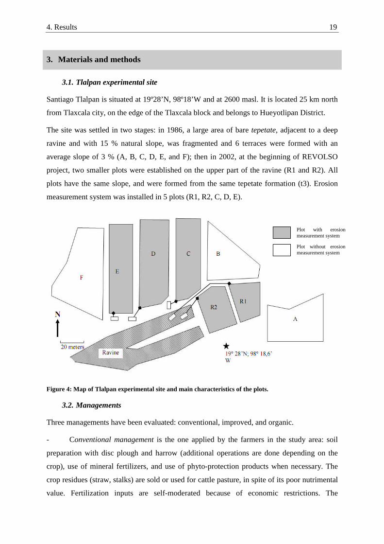
Santiago Tlalpan is situated at 19º28’N, 98º18’W and at 2600 masl. It is located 25 km north
from Tlaxcala city, on the edge of the Tlaxcala block and belongs to Hueyotlipan District.
The site was settled in two stages: in 1986, a large area of bare tepetate, adjacent to a deep
ravine and with 15 % natural slope, was fragmented and 6 terraces were formed with an
average slope of 3 % (A, B, C, D, E, and F); then in 2002, at the beginning of REVOLSO
project, two smaller plots were established on the upper part of the ravine (R1 and R2). All
plots have the same slope, and were formed from the same tepetate formation (t3). Erosion
measurement system was installed in 5 plots (R1, R2, C, D, E).
Figure 4: Map of Tlalpan experimental site and main characteristics of the plots.
3.2. Managements
Three managements have been evaluated: conventional, improved, and organic.
- Conventional management is the one applied by the farmers in the study area: soil
preparation with disc plough and harrow (additional operations are done depending on the
crop), use of mineral fertilizers, and use of phyto-protection products when necessary. The
crop residues (straw, stalks) are sold or used for cattle pasture, in spite of its poor nutrimental
value. Fertilization inputs are self-moderated because of economic restrictions. The
Plot with erosionmeasurement system
Plot without erosionmeasurement system

4. Results 20
incorporation of organic matter is low and is limited to the decomposition of roots and a
small part of the crop residues, since cattle usually graze the land after the harvest.
- Improved management is based on conventional management without restrictions of
inputs (all inputs required by the crop are applied), and use of associated crop (legumes)
when possible. All crop residues are incorporated to the soil, either whole or crushed. The
intention is to incorporate all organic matter available on the plot after harvesting, without
any addition of external sources such as manure or compost, and with minimum time and
work requirement.
- Organic management involves the same soil cultivation practices than the other
management systems, but with use of organic fertilization only (manure or compost) and
associated crop when possible. Crop residues are composted with additional farm manure and
then reincorporated to the soil. This management requires more time and labour, but provides
a higher level of incorporation of organic matter.
The plots fragmented in 1986 (A, B, C, D, E, F) were cultivated until 2002 under
conventional management. The main crops were maize and wheat, without any external
application of organic matter.
Table 2: Characteristics of Tlalpan experimental plots
Plot Management Year offragmentation
Label Surface(m2)
Erosion measurementsystem
A Improved 1986 1170 NoB Conventional 1986 1070 NoC Improved 1986 86-I 1630 YesD Organic 1986 86-O 2020 YesE Conventional 1986 86-C 1340 YesF Organic 1986 2200 No
R1 Conventional 2002 02-C 580 YesR2 Organic 2002 02-O 760 Yes
3.3. Crops and fertilization
Crops and fertilization applied from 2002 to 2005 are presented in table 3 and 4.
Table 3 : Crops cultivated from 2002 to 2005 at Tlalpan experimental site during the investigation.
Management 2002 2003 2004 2005
Improved Broad bean Oat + vetch Maize + bean Wheat
Conventional Broad bean Oat Maize + bean Wheat
Organic Broad bean Oat + vetch Maize + bean Wheat
Broad bean: Vicia fava; Vetch: Vicia sativa; Maize: Zea mays; Oat: Hordeum vulgare; Wheat:Triticum aestivum; Bean: Phaseolus vulgaris.

4. Results 21
Table 4: Fertilization applied from 2002 to 2005 at Tlalpan experimental site during the investigation.
Fertilization (N-P2O5-K2O, kg ha-1)
Plot Management 2002 2003 2004 2005
A Improved 60-100-34 23-60-00 98-41-00 82-23-00
B Conventional 23-00-00 23-00-00 81-00-00 62-23-00
C Improved 60-100-34 23-60-00 98-41-00 82-23-00
D Organic 6.8 t ha-1 (C) 3 t ha-1 (FYM) 1.9 t ha-1 (C) 3 t ha-1 (C)
E Conventional 23-00-00 23-00-00 81-00-00 62-23-00
F Organic 6.8 t ha-1 (C) 3 t ha-1 (FYM) 1.9 t ha-1 (C) 3 t ha-1 (C)
R1 Conventional 23-46-00 23-00-00 81-00-00 62-23-00
R2 Organic 6.3 t ha-1 (FYM) +crop incorporation*
3 t ha-1 (FYM) 2.6 t ha-1 (C) 4.2 t ha-1 (C)
FYM: Farmyard manure (dry matter); C: compost (dry matter); Vetch: Vicia sativa.* the broad bean was not harvested and the whole biomass was incorporated
3.4. Methods
3.4.1. Soil loss and runoff
The study has been performed on large farmers’ fields and under natural climatic conditions.
The initial erosion measurement system was designed by Fechter-Escamilla et al. (1995) and
has been described by Haulon et al. (2003). It consists of a one-foot H-flume (Hudson, 1993)
placed at the outlet of the field, and equipped with a water level recorder (OTT Thalimedes®
shaft encoder) set up at one minute time-step interval. Water level (mm) was converted into
flow discharge (m3 min-1) based on conversion table given in the Field Manual for Research
in Agricultural Hydrology (Brakensiek et al., 1979). After passing through the flume, runoff
discharge is channelled to a high capacity rotating tank (2 to 4.5 m3) set on 4 electronic
weight cells. In case the volume of runoff exceeds the capacity of the tanks, a hose connected
to a plastic reservoir collects an aliquot of the overflow. The original system (Fechter-
Escamilla et al., 1995) was developed to calculate soil loss according to the following
formula:
watersoil
soiltanktanktankin the
)(WeightSoil
VW(1)
With δ: density, W: weight of the slurry in the tank and V: volume of the slurry in the tank
However, in practice, weight and volume measurement are not precise enough to obtain a
reliable calculation of soil loss. Indeed, the average soil weight collected in the tanks ranged
from 10 to 20 kg. Considering that the precision of the weight cells is approximately 1%, the
standard error for a full tank (2 and 4.5 m3) is 20 to 45 kg, and the calculation is therefore

4. Results 22
strongly biased. As a consequence, this method was not used. Instead, soil loss was calculated
using a method of sediment concentration calculation as follows:
i. The heaviest fraction of soil particles tend to settle rapidly in accordance with Stoke’s law.
By the time samples are collected, the day after the storm event, the heaviest particles have
settled at the bottom of the tank, and it is not possible to homogenize the whole slurry and
maintain the heaviest particles in suspension to take representative samples. Therefore, the
“suspended” and “settled” sediments were treated separately.
ii. The “suspended” sediment fraction was homogenized by manual agitation during one
minute without disturbing the “settled” sediment fraction, and 1 dm3 sample was taken
immediately at 30 to 50 cm depth. The suspended fraction was then emptied by rotation of
the tank. The settled fraction was then collected, its volume was measured and 1 dm3
sample was taken. The sampling method was tested to evaluate the reproducibility of the
protocol. Results showed no significant differences in sediment concentration between
position and depth of sampling.
iii. In case the volume of runoff exceeded the capacity of the tank, a sample was collected from
the plastic reservoir.
iv. The water level in the flume was recorded by OTT Thalimedes® shaft encoder set up at one
minute time step interval. Water level (mm) was converted into flow discharge (m3 min-1)
based on conversion table given in the Field Manual for Research in Agricultural
Hydrology (Brakensiek et al., 1979).
v. Samples were oven-dried in the laboratory and their sediment concentration was
determined.
vi. Total soil loss was calculated as follow:
Wtotal = Wsuspended + Wsetted + Wout tank (2)
Soil weight (W) in each fraction equals the volume (V) of that fraction multiply by its
sediment concentration, with:
Vsuspended = Vin tank - Vsettled (3)
Vout tank = Vtotal at field outlet - Vin tank (4)

4. Results 23
Statistical analysis
Two issues must be considered:
i. The plots reclaimed in 1986 are larger than the plots reclaimed in 2002. On one hand, plot
length could increase flow velocity and particle detachments and as a result increase soil
erosion. On the other hand, larger plots may present more depositional areas and, hence,
reduce net erosion. Given our experimental design it is not possible to statistically control
possible size effect, and we will assume the effect of plot size is negligible.
ii. Given the cost of the erosion measurement system and the lack of tepetates available for
rehabilitation on the same experimental site (comparison between treatment should be done
only under same climatic conditions), no replicates are available. Each combination of age
of rehabilitation and management is only represented once.
To compare soil loss and water losses between plots, analysis of variance was performed
considering all erosive events1 within a year. Since soil losses are not normally distributed,
the base-10 logarithm of individual event soil loss value (E) was used. Since some events did
not produce soil loss (E) in all plots, the ANOVA was performed on LOG10(E+1).
3.4.2. Rain erosivity
Rainfall was recorded by mechanical daily recording rain gauge (pluviograph) during the
rainfall season from 2002 to 2005. In addition, a meteorological station was installed in 2003,
and precipitations were recorded with a tipping bucket rain gauge at a constant time step of 1
minute. However, the precision of the device failed, and in 2004 a Hobo® event recorder
connected to a tipping-bucket rain gauge was installed, allowing a precise calculation of
rainfall intensity and kinetic energy. The combination of recording devices ensures continuity
of records in case of failure.
Rain kinetic energy was calculated using the equation proposed by van Dijk et al.(2002):
Ek=28.3[1-0.52(-0.042I)] (5)
Where Ek is the kinetic energy in J m-2 mm-1 for a time lap of constant intensity.
The total rainfall or storm kinetic energy is the sum of the product of each time lap kinetic
energy and the rain depth during this time lap:
1 We took into account all events that produced soil loss in at least one plot.

4. Results 24
t
n
t REkE 1(6)
E is the total rainfall energy
Ekt is the kinetic energy of a constant intensity time lap t
Rt is the rain depth during a constant intensity time lap t
n is the number of constant intensity time laps during the rainfall
The annual kinetic energy is the sum of all rainfall event’s kinetic energy.
The van Dijk formula was compared to the equation proposed by Renard et al. (1997) for the
RUSLE which is adapted from earlier formulation by Wischmeier and Smith (1958):
Ek = 11.9+8.73 log10I if I ≤ 76 mm h−1(7)
Ek = 28.3 if I > 76 mm h−1(8)
3.4.3. Vegetation cover
In 2002 and 2003, vegetation cover was measured by a simple version of quadrat sighting
frame (Stocking, 1994), consisting of a board perforated with fifty 2 mm-diameter holes at 2
cm interval. The amount of bare ground visible through the hole was quantified from 0 (bare
soil) to 5 (totally covered by vegetation). The nature of the cover was also qualified (main
crop, associated crop, residues, weeds). However, difficulties with crop height,
representativity in case of raw crops and observers variability, also reported by Stocking
(1994), led to reduced reliability of the measurements. Consequently, in 2005, a new method
based on digital photograph taken at 7 meters height and analyzed by image processing
software was developed and used. This method discriminates plant area from soil area by
binarization processing. In 2004, only visual observation was performed at maximum
development stage of the crop.
Repeated measures ANOVA was performed and Tukey HSD at 0.05 confidence level was
used to compare treatments.
3.4.4. Aggregate stability
3.4.4.1.Percolation stability
After the works of Sekera and Brunner (1943) and Becher and Kainz (1983), Kainz and Weiss
(1988) developed a method to assess aggregate stability based on the percolation of water
through a column of calibrated aggregates. The aggregates are placed in a 100 mm-long tube

4. Results 25
with an inside diameter of 15 mm. Deionised water is then percolated during 10 minutes
under a hydrostatic head pressure of 20 hPa. The amount of water percolated is regarded as
the percolation stability (PS) index.
The principle driving the percolation stability (PS) test is the obstruction of the pores by
displacement and re-organisation of the microaggregates and particles resulting from the
aggregates breakdown, thereby reducing the amount of water that passes through the column.
In this method, since the aggregates are previously air dried and rapidly wetted, Auerswald
(1995) stated that the aggregate breakdown occurs mainly by compression of trapped air
during wetting (slaking). The magnitude of the breakdown depends on the strength of the
cohesive forces holding the aggregate. High values indicate high aggregate stability.
The original test is performed on 1-2 mm diameter air-dried aggregates. In this study, the
method was widened and the test was performed on three aggregate sizes: 0.59-1 mm, 1-2
mm, and 2-3.15 mm. The interest was to evaluate the stability of a wider range of aggregate
size so that the sample tested is more representative to the whole soil behaviour (Loch, 1994).
Based on this consideration, the weighted PS (PSw) was calculated to take into account the
relative proportion of each aggregate size class.
xWPSxPSw ( 9)
With PSx = Percolation stability index for aggregate size x
Wx = Fraction of aggregate size x in relation to the other aggregate sizes tested.
3.4.4.2.Aggregate size distribution
Large samples were taken in field and air dried at room temperature in laboratory. Samples
were then sieved through a column of 7 meshes at 10, 8, 5, 3.15, 2, 1 and 0.59 mm in a rotary
sieve device during 4 minutes. The aggregates caught on each sieve were weighted and the
fraction of each size was calculated. The fraction >10 mm was not considered in the
calculation as this size of aggregate is very variable and can affect artificially the final
aggregate size distribution. The mean weight diameter (MWD) (Nimmo and Perkins, 2002),
was then calculated. Greater MWD implies greater stability.
In dry-sieving procedure, the disruptive agent responsible for the aggregate breakdown is the
mechanical energy produced by the collision between the aggregates and the sieve or

4. Results 26
between aggregates themselves. One measure was performed for each sample. Over the 3
years, the sample (< 10 mm) mean weight was 1048 g (standard deviation=318, n=130).
3.4.4.3.Sampling
The sampling and processing differ from one year to another (Table 5). Therefore, the results
are not compared between years, but only within a year.
Table 5: Method and sampling details for soil aggregation assessment in Tlalpan.
2003 2004 2005
Date of sampling November 2003 November 2004 13/07/2005
22/09/2005
17/11/2005
Date of testing February 2004 March 2006 August 2005October 2005December 2005
Plots all all Erosion plots(C, D, E, R1, R2)
Field sampling 2 samples at 3positions (top,medium and low partof the plot)
1 compound samples (4 sub-samples) at2 positions: ridge + furrow
1 compound sample (6sub-samples)
Depth 0 – 10 cm 0 – 10 cm 0 – 10 cm
Aggregate size 1 – 2 mm 0.59 – 1 mm 0.59 – 1 mm
tested 3.15 – 5 mm 1 – 2 mm 1 – 2 mm
2 – 3.15 mm 2 – 3.15 mm
Replicate 3 3 3
N total 288 144 135
3.4.4.4.Statistical analysis
Between groups analysis of variance (ANOVA) was performed using SPSS (SPSS Inc.).
Tukey (Honestly Significant Difference) test at 95 % confidence was used for multiple
comparisons.
3.4.5. Particle size distribution
Particle size distribution was determined by Laser diffraction (LD) technique on a Beckman-
Coulter LS 230 at the School of Geography of the University of Nottingham. Laser
diffraction technology have been used in several studies for soil particle size distribution
(PSD) in the last 10 years (Buurman et al., 1997; Muggler et al., 1997; Konert and
Vandenberghe, 1997; Beuselinck et al., 1998; Chappell, 1998; Westerhof et al., 1999; Eshel
et al., 2004). The theory behind laser diffraction (or light scattering) technique have been
extensively described by these authors and is provided by the manufacturer (Coulter, 1994).

4. Results 27
Apart from the short time analysis required for LD, the main advantage of this technique is
that it provides continuous PSD over a wide range of size fraction.
The Fraunhofer optical model was used for calculation and the PIDS (polarization intensity
differential of scattered light) module was not used. PSD was measured over the range of
0.375 µm to 2000 µm. The protocol to prepare samples previous to their analysis in the fluid
module was as follow:
0.15 to 0.2 g of soil was put in 10 ml hydrogen peroxide (10 % H2O2) for 1 hour and was then
heated progressively for 2 hours to destroy all organic compounds. The sample was allowed
to cool and 25 ml distilled water was added. The sample was then centrifuged at 3500 rpm for
5 minutes and the liquid in excess was poured out gently. Another 25 ml distilled water was
added and the sample was centrifuged again to rinse all the remaining peroxide. The liquid
was poured and 25 ml Calgon was added. The sample was shaken manually for 1 minute and
then placed in an ultrasonic bath for at least 30 minutes before being analyzed in the fluid
module containing tap water. Three replicates of each soil were analyzed. Given the high
reproducibility between runs (+- 2 %), only one run of 1 minute was performed for each
replicate.
PSD by the hydrometer method was also performed in the laboratory of soils of the
Autonomous University of Tlaxcala following the protocol proposed by Gee and Or (2002).
LD particle size distribution between plots were compared by ANOVA repeated measures.
3.4.6. Porosity and pore size distribution
Total porosity was determined by gravimetric method with water saturation (Flint and Flint,
2002) and pore size distribution by water desorption method (Flint and Flint, 2002), at 2.45,
5.88, 9.8, 33, 100 and 1500 kPa. Total porosity means were compared by ANOVA (Tukey at
0.05), and water retention curve (pore size distribution) were compared by repeated measures
ANOVA.
3.4.7. Soil Organic Carbon
In each plots, two composite samples from 10 sub-samples were taken at 0-10 cm depth at
the end of the rainy season. Soil organic carbon was measured by dry combustion in a
Carmograph 8 Wösthoff at the laboratory of soil science of the Colegio de Postgraduados.
Samples were measured once. The precision of the measures was verified by running
standard control samples regularly.

4. Results 28
4. Results
4.1. Erosivity and soil erosion
4.1.1. Rainfall erosivity
Results presented in this part are based on records from 2002-2005 taken during REVOLSO
project, and unpublished records from 1991 to 1997 recorded during previous projects by
Jürgen Baumann and Ulrich Fechter-Escamilla and colleagues from the University of
Tlaxcala.
4.1.1.1.Annual precipitation
Mean annual precipitation over the period 1991-2005 in Tlalpan was 670 mm. Values ranged
from 530 mm (2002) to 805 mm (2003), with a standard deviation of 108 mm. Data recorded
over the 2002-2005 period are consistent with those recorded previously over the 1991-1997
period. There is no significant difference (p<0.05) between the mean annual precipitation for
the two periods (660 and 675 mm respectively)
Table 6: Annual precipitation and R factor in Tlalpan, Tlaxcala.
year Precipitation R (EI30)
(mm) (N h-1)1991 804 3581992 803 2721993 663 2111994 719 4351995 603 197
1996 607 2181997 553 N/A2002 530 1842003 805 3452004 756 3772005 577 195Mean 675 127
Beside their proximity (3 geographic minutes), Tlalpan appears to be drier than Hueyotlipan,
with 105 mm less precipitation in average. Part of this difference is attributed to the fact that
winter precipitations were not recorded consistently in Tlalpan. However, the trend confirms
the great spatial climatic variability in Tlaxcala (Conde et al., 2006; Eakin, 2000).
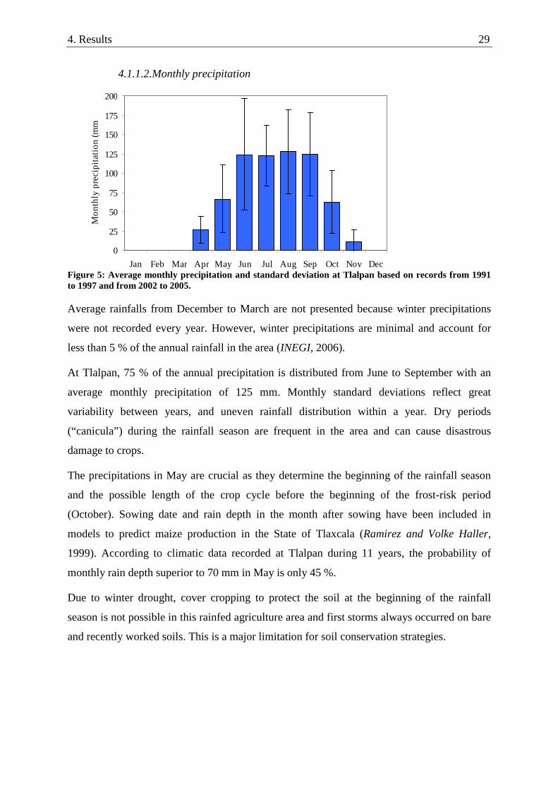
4. Results 29
4.1.1.2.Monthly precipitation
0
25
50
75
100
125
150
175
200
Jan Feb Mar Apr May Jun Jul Aug Sep Oct Nov Dec
Mo
nth
lyp
reci
pit
atio
n(m
m)
Figure 5: Average monthly precipitation and standard deviation at Tlalpan based on records from 1991to 1997 and from 2002 to 2005.
Average rainfalls from December to March are not presented because winter precipitations
were not recorded every year. However, winter precipitations are minimal and account for
less than 5 % of the annual rainfall in the area (INEGI, 2006).
At Tlalpan, 75 % of the annual precipitation is distributed from June to September with an
average monthly precipitation of 125 mm. Monthly standard deviations reflect great
variability between years, and uneven rainfall distribution within a year. Dry periods
(“canicula”) during the rainfall season are frequent in the area and can cause disastrous
damage to crops.
The precipitations in May are crucial as they determine the beginning of the rainfall season
and the possible length of the crop cycle before the beginning of the frost-risk period
(October). Sowing date and rain depth in the month after sowing have been included in
models to predict maize production in the State of Tlaxcala (Ramirez and Volke Haller,
1999). According to climatic data recorded at Tlalpan during 11 years, the probability of
monthly rain depth superior to 70 mm in May is only 45 %.
Due to winter drought, cover cropping to protect the soil at the beginning of the rainfall
season is not possible in this rainfed agriculture area and first storms always occurred on bare
and recently worked soils. This is a major limitation for soil conservation strategies.

4. Results 30
4.1.1.3.Rainfall patterns in Tlalpan
0%
2%
4%
6%
8%
10%
12%
14%
0 1 2 3 4 6 7 8 9 10 11 12 13 14 15 16 17 18 19 20 21 22 23
Start time (hour)
Pe
rce
nta
ge
ofe
ve
nts
>1
mm
Figure 6: Start time of rainfall events (> 1mm) between 2002 and 2005 in Tlalpan
Over the 2002-2005 period, 360 events separated by at least 60 minutes and with a minimum
precipitation of 1 mm were recorded. 71 % of the events started in the afternoon and evening
between 14:00 and 20:00, with 51 % of the events concentrated between 15:00 and 18:00.
This pattern reflects the dominance of convective rainfalls which are characteristic in
Mexican highlands (Prat, 1997) and more generally in continental highlands (Nyssen et al.,
2005).
Table 7: Mean selected characteristic of rainfall events in Tlalpan over the 1991-2005 period (2003-2005for soil loss). See Table A- 1 for annual details.
Max I30 Soil loss
count % mm % N h-1 % mm h-1 %Mean < 1mm 57.6 40.1% 20.5 3.0% 0.4 0.1% 0.8
1-4.99 mm 43.8 30.5% 108.0 16.0% 8.3 3.0% 3.5 0.3%5-9.99 mm 19.6 13.7% 142.0 21.0% 25.6 9.2% 8.7 4.3%
10-19.9 mm 16.8 11.7% 236.2 35.0% 87.7 31.4% 16.1 36.1%20-29.9 mm 3.9 2.7% 92.9 13.8% 58.9 21.1% 26.1 15.9%
> 30 mm 1.8 1.3% 75.1 11.1% 98.3 35.2% 50.0 43.4%
Max rainfall 45.6 6.8% 63.0 22.5% 40.6 13.9%Total 143.6 674.6 279.2
EI30DepthEvents
Rain events < 1mm represented on average 40 % of the events, but only accounted for 3 % of
the annual precipitation. There were more numerous over the 2002-2005 period than over the
1991-1997 period because of the precision of the recording device (tipping bucket and event
recorder) which allowed to record numerous isolated pseudo-events that were not perceptible
on the daily pluviograph used between 1991 and 1997.
The number of events is inversely proportional to the size of the event. Events up to 10 mm
represented 84 % of the events, 40 % of the annual precipitation, but only contributed to 12
% of the annual erosivity (EI30) and produce 4.3 % of soil loss. Rainfall events of 10-20 mm

4. Results 31
contributed to 35 % of the annual precipitation. Such events were on average less intense
(16.1 mm h-1 in 30 minutes) than those of 20-30 mm (26 mm h-1) but they are more numerous
and all together accounted for 36.1 % of the annual erosivity against only 15.9 % for events
20-30 mm. Events >30 mm only occur on average 1.8 time per year and account for 11 % of
the precipitation. However, they were the most intense (50 mm h-1 maximum I30 on
average), they produced 35 % of the erosivity and 43.4 % of the annual soil loss. Maximum
rainstorm depth ranged from 31 to 67.1 mm over the 1991-1997 period and from 32.7 to 63.8
mm over the 2002-2005 period. The biggest rainstorm is not always the most erosive event,
as erosion also depends on the soil condition (protection, roughness, water saturation, etc.) at
the moment on the storm.
4.1.2. Runoff and soil loss
Figure 7: Annual soil loss, runoff, runoff coefficient and sediment discharge in Tlalpan from 2003 to 2005.See Table A- 2 for details.
In recently reclaimed tepetates erosion rates ranged from 5.5 to 14.1 t ha-1 yr-1 in organic
management (02-O) and from 8.6 to 19.1 t ha-1 yr-1 in conventional management (02-C).
Over the period, soil loss in conventional management was significantly (p<0.05) greater than
in organic management, with a difference of 3.1 to 5 ton ha-1 yr-1 (Table A- 2).
0
5
10
15
20
Soil
loss
(tha
-1)
2003
2004
2005
0
50
100
150
200
250
Runoff
(mm
)
0
20
40
60
80
86-I 86-O 86-C 02-C 02-O
Sedim
entd
isch
arg
e(k
gm
m-1)
0%
10%
20%
30%
40%
50%
86-I 86-O 86-C 02-C 02-O
Runoff
coeffic
ient
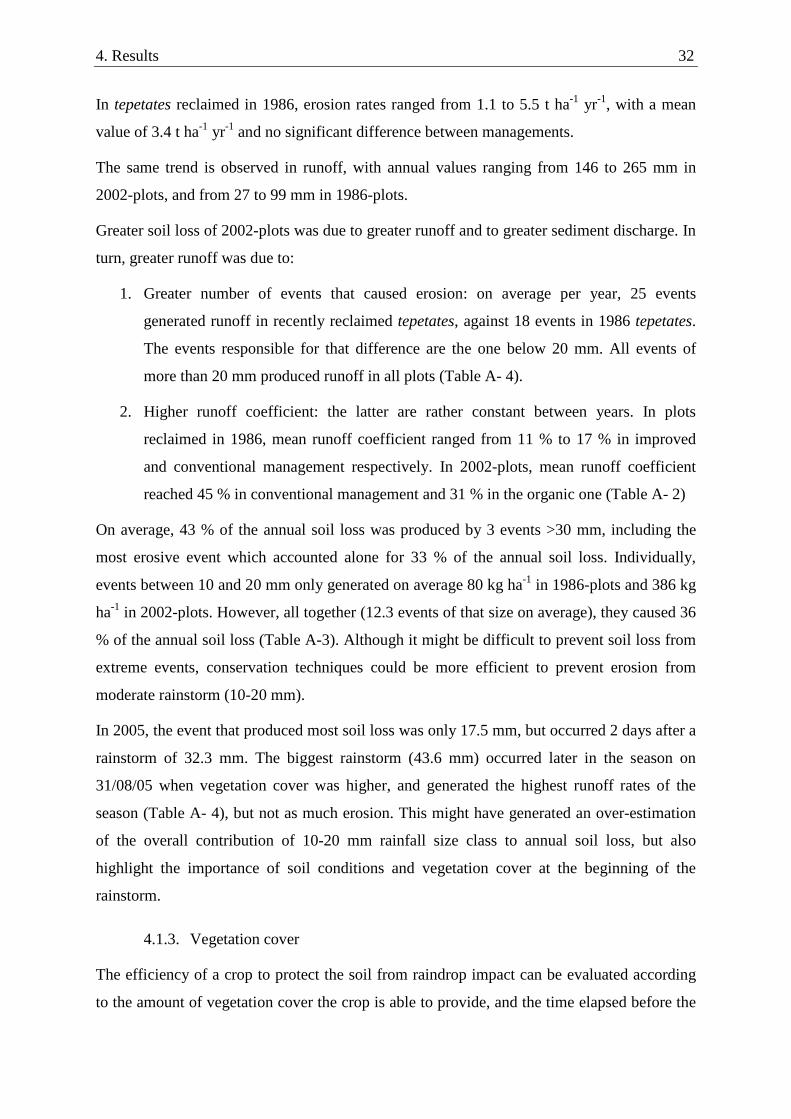
4. Results 32
In tepetates reclaimed in 1986, erosion rates ranged from 1.1 to 5.5 t ha-1 yr-1, with a mean
value of 3.4 t ha-1 yr-1 and no significant difference between managements.
The same trend is observed in runoff, with annual values ranging from 146 to 265 mm in
2002-plots, and from 27 to 99 mm in 1986-plots.
Greater soil loss of 2002-plots was due to greater runoff and to greater sediment discharge. In
turn, greater runoff was due to:
1. Greater number of events that caused erosion: on average per year, 25 events
generated runoff in recently reclaimed tepetates, against 18 events in 1986 tepetates.
The events responsible for that difference are the one below 20 mm. All events of
more than 20 mm produced runoff in all plots (Table A- 4).
2. Higher runoff coefficient: the latter are rather constant between years. In plots
reclaimed in 1986, mean runoff coefficient ranged from 11 % to 17 % in improved
and conventional management respectively. In 2002-plots, mean runoff coefficient
reached 45 % in conventional management and 31 % in the organic one (Table A- 2)
On average, 43 % of the annual soil loss was produced by 3 events >30 mm, including the
most erosive event which accounted alone for 33 % of the annual soil loss. Individually,
events between 10 and 20 mm only generated on average 80 kg ha-1 in 1986-plots and 386 kg
ha-1 in 2002-plots. However, all together (12.3 events of that size on average), they caused 36
% of the annual soil loss (Table A-3). Although it might be difficult to prevent soil loss from
extreme events, conservation techniques could be more efficient to prevent erosion from
moderate rainstorm (10-20 mm).
In 2005, the event that produced most soil loss was only 17.5 mm, but occurred 2 days after a
rainstorm of 32.3 mm. The biggest rainstorm (43.6 mm) occurred later in the season on
31/08/05 when vegetation cover was higher, and generated the highest runoff rates of the
season (Table A- 4), but not as much erosion. This might have generated an over-estimation
of the overall contribution of 10-20 mm rainfall size class to annual soil loss, but also
highlight the importance of soil conditions and vegetation cover at the beginning of the
rainstorm.
4.1.3. Vegetation cover
The efficiency of a crop to protect the soil from raindrop impact can be evaluated according
to the amount of vegetation cover the crop is able to provide, and the time elapsed before the

4. Results 33
cover is developed. The amount of vegetation cover depends on i) the type of crop, mainly
responsible for mean differences between years, and ii) crop development, which depends on
the management applied and which is mainly responsible for differences between plots within
a year. Crop development depends on plant nutrition and water supply.
Results are presented in Table A- 5.
4.1.3.1. 2002
Among the crop rotation applied between 2002 and 2005, broad bean is the crop that
provided less vegetation cover to the soil. Maximum cover was reached after approximately
130 days after sowing, with soil covered up to 71 % (86-O) and 79 % (86-C) in 1986-plots,
and 44 % (02-O) to 41 % (02-C) in 2002-plots.
4.1.3.2. 2003
In 2003, the association between oat and vetch significantly increased vegetation cover to 84
% (86-I) compared to 61 % (86-C) with oat single cropping in 1986-plots, to 70 % (02-O)
compared 39 % (02-C) in plots reclaimed in 2002.
The analysis of the composition of the vegetation cover (Figure 7) clearly shows that:
i. On average over the season, vegetation cover by oat was similar between
management, ranging from 38 to 45 %.
ii. The vetch provided another 29 % vegetation cover in 02-O, and 21 % on average in
86-I and 86-O. There were not significant differences in vetch cover between plots
where this species was associated with oat (organic and improved).
iii. Vegetation cover was higher in plots reclaimed in 1986 because of adventives weeds
(18% of additional cover on average). In plots reclaimed in 2002, the amount of soil
covered by weeds is negligible since the material was still free of adventives seeds.
The maximum vegetation cover by oat occurred 54 days after sowing and decayed gradually
afterwards. Vetch development and cover was slower, but constant throughout the rainfall
season and until harvesting, approximately 100 days after sowing.
The association oat-vetch provided greater vegetation cover and over a larger period. This is
a substantial benefit in the study area where hurricane season usually generate strong erosive
events at the end of the growing season in September-October (See part 4.1.1).

4. Results 34
Figure 8: Composition of vegetation cover in 2003 in Tlalpan
Although vegetation cover was established rapidly after sowing, the biggest rainstorms
occurred at the beginning of the season when only 10 % of the soil (on average) was covered
and caused major soil loss (Figure 9).
Figure 9: Distribution of vegetation cover (average value from all plots), precipitation and soil loss(average value from all plots) during 2003 in Tlalpan.
0%
20%
40%
60%
80%
100%
0%
20%
40%
60%
80%
100%
0%
20%
40%
60%
80%
100%
14/07/03 14/08/03 14/09/03
Weeds
Vetch
Oat
0%
20%
40%
60%
80%
100%
14/07/03 14/08/03 14/09/03
86-C 86-O and 86-I
02-C 02-O

4. Results 35
4.1.3.3.2004
The evaluation of the vegetation cover was done at grain filling stage, approximately 100
days after sowing. Based on this observation, vegetation cover was higher in 86-I (87 %) than
in 86-O and 86-C (78 %). In recently reclaimed tepetates, 02-O reached 70 % cover, against
only 35 % in 02-C.
This observation confirmed the fertility limitations of recently reclaimed tepetates for maize
cropping under conventional management (Baumann and Werner, 1997b). However, it also
proved that from the third year after fragmentation, maize cropping can produce similar
yields (Table A- 7) and vegetation cover than reclaimed tepetates with several years of
rehabilitation, providing adequate plant nutrition is applied.
In 2004, the biggest rainstorm occurred in September during the hurricane season and caused
major soil loss although vegetation cover was already well established (Figure 10). It is a
clear illustration that vegetation cover can mitigate the effect of erosive event by protecting
the soil against raindrop impact, but has limited effect in case of extreme event when particle
detachment by overland flow is the dominant detachment mechanism.
Figure 10: Distribution of vegetation cover (predicted average value of all plots), precipitation and soilloss (average value of all plots) during 2004 in Tlalpan.
4.1.3.4. 2005
Thanks to the aerial photography method, we were able to monitor the vegetation cover
during the whole crop cycle. Over this period, 86-O and 86-I provided up to 90 % of soil
cover 100 days after sowing. 86-C was significantly lower with a maximum of 81 %. The

4. Results 36
plots reclaimed in 2002 suffered nutrition limitations and vegetation cover did not reach more
than 63 %. Over the period the difference between the two managements was not significant.
On average in plots reclaimed in 1986, wheat was able to provide more than 80 % soil cover
60 days after sowing and maintained this level during approximately 60 days, representing 46
% of the vegetative period (Figure 11). This level of vegetation cover was particularly
effective in mitigating soil loss for the two extreme rainstorms (over 40 mm) which occurred
in August (31st) and October (11th).
Figure 11: Distribution of vegetation cover (average value of all plots), precipitation and soil loss (averagevalue of all plots) during 2005 in Tlalpan
4.2. Soil properties and crop production
4.2.1. Soil Organic Carbon
The main difference between Conventional, Improved and Organic management is the
incorporation of organic matter (Cf chapter 3.3). The evolution of SOC content is an indicator
of the effect of management on carbon dynamic in tepetates.
In total, 5.6 Mg OM (biomass) ha-1 yr-1 and 6.8 Mg OM ha-1 yr-1 were incorporated over the
period in 86-O and 02-O respectively. Organic fertilization represented on average 63 % of
the annual incorporation rate, whereas crop residues accounted for 24% and roots for another
13 % of the amount of C incorporated each year in average (Table 8). In 86-I, the

4. Results 37
incorporation of organic material amounted 4.4 Mg OM ha-1 yr-1, of which 89 % was
provided by crop residues and 11% by roots. In 86-C, average incorporation rate was 2.5 Mg
OM ha-1 yr-1, with crop residues accounting for 67% of the total accumulation and roots for
33 %. In 02-O, only 1.1 Mg OM ha-1 yr-1 was incorporated, of which the major part (60 %)
came from roots (Table 8).
Table 8: Organic material (biomass) inputs and C accumulation rates in Tlalpan from 2002 to 2005 at 0-20 cm depth. OM inputs from roots were estimated from the work of Fechter-Escamilla et al. (1997b).
86-C 86-I 86-O 02-C 02-O2002 organic fertilziation - - 6.8 - 6.3
residues - - - - -roots - - - - -
2003 organic fertilziation - - 3.0 - 3.0residues n-1 (broad bean) - 3.2 - - 2.3aroots n-1 (broad bean) 1.1 1.1 1.1 1.1 1.1
2004 organic fertilziation - - 1.9 - 2.6residues n-1 (oat or oat + vetch) 3.8 3.3 2.9 1.2 3.9roots n-1 (oat or oat + vetch) 0.8 1.4 1.4 0.8 1.4
2005 organic fertilziation - - 3.0 - 4.3
residues n-1 (maize) 1.5 5.5 1.5 0.5 1.4roots n-1 (maize) 0.8 0.8 0.8 0.8 0.8
Total organic fertilziation - - 14.7 - 16.2residues 5.2 12.0 4.4 1.7 7.7roots 2.6 3.2 3.2 2.6 3.2
Total (Mg OM ha-1) 7.8 15.2 22.3 4.3 27.1
Incorporation rate (Mg OM ha-1 yr-1) 2.0 3.8 5.6 1.1 6.8
Incorporation rate (Mg C ha-1 yr-1)b1.0 1.9 2.8 0.5 3.4
Accumulation rate (Mg C ha-1 yr-1)c 0.21 0.37 0.61 0.22 0.80
Ratio accumulated/incorporated 21% 19% 22% 40% 24%a incorporated as green manureb with C = 1/2 OMc Cf table 12
In 86-C, where crop residues were exported and no organic material was incorporated, SOC
content (0-20 cm depth) increased by 0.36 mg g-1 over the period (Table 9), indicating that
after more than 15 years of cultivation after fragmentation and with reduced inputs of O.M,
SOC keeps increasing under conventional management. In 86-I, where residues were
incorporated, SOC increased by 0.61 mg g-1 over the period. In 86-O, where residues were
composted and organic fertilization was applied, SOC increased by 1.01 mg g-1. In 02-O, the
incorporation of manure after fragmentation and the incorporation of the green manure (broad
bean) produced an increase of 0.77 mg g-1 within the first year after fragmentation. Over the 4
years period with regular but reasonable organic matter inputs (Table 8) SOC increased by
1.34 mg g-1. In 02-C with no organic matter incorporation apart from roots and residues, SOC
increased by 0.36 mg g-1 (Table 9).
Organic farming after fragmentation increased carbon sequestration rates to equivalent 0.80
Mg C ha-1 yr-1 compared to 0.22 Mg C ha-1 yr-1 in conventional farming.

4. Results 38
Table 9: Soil Organic Carbon (mg g-1) and accumulation rate at 0-20 cm depth in Tlalpan from 2002 to2005. Data at 0-10 and 10-20 cm depth are presented in Table A- 6 in Appendix 7.
2002 2003 2004 2005 Δ 02-05 mg C g-1 yr-1 Mg C ha-1 yr-1
86-C 2.99 3.70 3.40 3.34 0.35 0.09 0.2186-I 3.21 3.50 3.83 3.83 0.61 0.15 0.3786-O 3.09 4.42 4.78 4.10 1.01 0.25 0.6102-C 1.08 0.81 1.45 1.43 0.36 0.09 0.2202-O 1.08 1.84 2.20 2.41 1.34 0.33 0.80
ManagementSOC (mg g-1) Accumulation rates
4.2.2. Soil water content
In 2004 soil moisture was assessed by TDR from sowing to mid-September. Measurements
were not continued due to failure of the device. In 2004, no significant differences were
observed between treatments (Figure 12).
5%
15%
25%
10-July 10-August 10-September
Wat
erco
nte
nt(v
olu
met
ric) 86-I
86-O
86-C
02-C
02-O
0
10
20
30
Pre
cipitat
ion
(mm
)
Figure 12: Monitoring of soil water content (volumetric) at 10 cm depth by TDR during 2004 croppingseason. Cf Table A- 8.
In 2005, soil moisture was assessed by tensiometers on a regular basis (32 measurements).
Over the period, soil water content was significantly lower in 02-plots (mean value of 23 %)
than in 86-I and 86-C (Mean value of 33 %) (Figure 13 and Table A- 9)

4. Results 39
10%
20%
30%
40%
01-July 01-August 01-September 01-October 01-November
Wat
erco
nte
nt(g
ravim
etri
c)
86-I
86-O
86-C
02-C
02-O
0
10
20
30
40
Pre
cipit
atio
n(m
m)
Figure 13: Monitoring of soil water content (gravimetric) by tensiometers during 2005 cropping season(weighted average from measures done at 5, 10, 15, 25 and 40 cm depth). Cf Table A- 9.
4.2.3. Crop production
Crop production and vegetation cover are strongly related, since both parameter depends on
crop development. Crop yields are presented in Table A- 7, to support the discussion on the
effect of management on vegetation cover.
4.3. Soil structure
4.3.1. Particle size distribution
Table 10: Particle size distribution in Tlalpan experimental site’s plots.
Clay
< 2 µm 2 - 20 µm 20 - 50 µm 2 - 50 µm 50 - 250 µm 250 - 500 µm 500 - 2000 µm 50 - 2000 µmA 6.3 31.3 13.1 44.4 35.5 10.0 3.9 49.3B 7.7 34.5 14.0 48.5 31.1 9.0 3.7 43.9C 7.6 35.8 14.3 50.1 29.7 9.2 3.4 42.3D 8.2 34.0 13.4 47.3 30.7 9.6 4.2 44.5E 9.1 38.7 11.8 50.6 27.6 9.2 3.6 40.4F 9.9 35.0 11.5 46.5 29.1 10.3 4.3 43.7R1 10.7 37.7 10.8 48.5 26.7 9.8 4.4 40.9R2 9.5 37.3 13.1 50.4 28.7 8.7 2.8 40.1Mean 8.6 35.5 12.7 48.3 29.9 9.5 3.8 43.1
SandsSilt
The average texture is 8.6 % clay (<2 µm), 48.3 % silt (2 - 50 µm) and 43.1 % sand (50 –
2000 µm). The most represented fraction is fine silt-size (2 – 20 µm) particles, accounting for
35.5 % of the soil volume on average. Very fine and fine sands accounted for 29.9 % of the
soil volume, whereas coarse and very coarse sands (<500 µm) only accounted for 3.8 % of

4. Results 40
the soil. There were no significant differences in particle size distribution between plots
(ANOVA repeated measures).
LD PSA revealed the bimodal particle distribution with a peak at 5 µm and another one at
100 µm (Figure 14)
0
0.5
1
1.5
2
2.5
0.1 1 10 100 1000 10000Particle size (µm)
%of
Volu
me
86-I
86-O
86-C
02-C
02-O
Clay: < 2µm Silt: 2 - 50 µm Sand: 50 - 2000
µm
Figure 14: Particle size distribution measured by Laser Diffraction in Tlalpan in plots where erosion wasmeasured.
Soil texture classification systems were developed for PSD obtained by sieving-
sedimentation methods. No classification systems exist yet for PSD obtained by LD and it is
therefore necessary to convert LD PSD to pipette or hydrometer PSD in order to define the
soil texture class. According to LD PSD, reclaimed tepetates in Tlalpan would be clay loams
(USDA classification).
Laser diffraction grain analysis tends to underestimate clay content in comparison to the
sieve-pipette method more conventionally used (Beuselinck et al., 1998; Konert and
Vandenberghe, 1997; Eshel et al., 2004). This distortion is due to the fact that both methods
do not measure the same property of the same material. The laser diffraction analysis
determines the diameter of a particle whose diffraction is equivalent to the one of a sphere
(optical-equivalent diameter). Gravitational sedimentary pipette method determines the
diameter of a particle whose settling velocity is equivalent to the one of a quartz sphere
(spherical-equivalent diameter).
Because clays are platy particles, their average optical diameter is much greater than their
equivalent spherical diameter. Konert and Vandenberghe (1997) showed that some particles

4. Results 41
with a clay spherical-equivalent diameter of 2 m (from pipette method) have a optical-
equivalent diameter of 3.9 μm. Much of the material measured as clay by the pipette method
is therefore measured as silt on the diffraction method. Since coarse silt and sand spherical
and optical diameters are similar, there is a good relationship between pipette and laser
diffraction method for sands content (Beuselinck et al., 1998; Konert and Vandenberghe,
1997; Eshel et al., 2004). However, because of the underestimation of clays, silt fraction
tends to be largely overestimated. To convert particle size distribution obtained by LD to
values obtained by sieve-pipette, two methods have been proposed:
i. Konert and Vandenberghe (1997) proposed that clay (<2 μm) content by sieve-pipette
method be equivalent to particles size <8 m measured by laser diffraction.
ii. Beuselinck et al. (1998) proposed to estimate clay and sand content using RMA regression
equations:
For clay (< 2 m): y = 2.744x – 7.773
For sand (> 63 m): y = 1.155x – 6.105
And then calculate silt content as 100 – (% estimated clay + % estimated sand).
Table 11: Measured and corrected texture obtained by LD and pipette methods in Tlalpan.
Method % Clay % Silt % Sands
< 2 µm 2 - 50 µm 50 - 2000 µm
LD (Coulter LS 230) 8.6 48.3 43.1
Hydrometer 32.5 25.8 41.8
LD Corrected (Beuselinck) 15.9 40.4 43.7
LD Corrected (Konert) 30.5 26.4 43.1
Sieve-pipette (Covaleda, 2007) 33.7 30.0 36.4
Sieve-pipette (Baumann, 1996) 26.9 35.0 38.1a Baumann used sands > 63 m. Silt fraction is therefore overestimated compared to the USDA classification, and sandfraction underestimated.b RMA relationship for sands was calculated by Beuselinck for sands > 63 m.
Hydrometer PSD is in the range of the pipette PSD reported by Covaleda et al (2007), with a
difference of 1.2 % in clay content and 4.4% in sand content. However, it differs from pipette
PSD reported by Baumann (1996) (Δ clay: 5.6 % and Δ sands: 3.7 %). Part of this difference
is due to the fact that the upper limit for silt fraction was 63 µm and induced an
overestimation of silt fraction (Δ = 9.2 %).

4. Results 42
The correction proposed by Konert and Vandenberghe (1997) (increasing the limit of clay
fraction to 8 m) gave a good approximation of the equivalent pipette PSD, with differences
of less than 2 % in each size fraction compared to hydrometer PSD.
The correction proposed by Beuselinck et al. (1998) did not predict satisfactorily the clay
content measured by the hydrometer method, with a difference of 16.6 %. The RMA
relationships defined by Beuselinck et al. (1998) were based on 83 samples derived from
natural silt and modified to obtain a wide range of texture. However, the clay fraction used in
their experiment consists mainly of illite and smectite, whereas clays minerals in tepetates are
mainly halloysite and cristobalite (Peña and Zebrowski, 1992a). This may have created a bias
since relationships between LS and pipette methods are affected by clay mineralogy and
morphology (Beuselinck et al., 1998).
It is important to highlight that all methods suffer from inherent flaws (Eshel et al., 2004) and
none can be considered as absolutely correct.
4.3.2. Aggregation
4.3.2.1.Dry aggregate size distribution
The smallest aggregate fraction (<0.59 mm) is the predominant fraction and represented on
average 31% of the soil sample (> 10 mm). There is a significant difference (p<0.001) in the
fraction of aggregates size >1 mm between 1986-plots (34.8 %) and 2002-plots (42.3 %)
(Table A- 15). This feature reflects a lower aggregation of the finer particles in the recently
rehabilitated tepetates, which is also expressed by smaller MWD over the period. All other
aggregate-size fraction ranged between 10 % and 15 % of the soil (< 10 mm).
In 2003, MWD are higher because the smallest mesh size was 1 mm, whereas in 2004 and
2005, samples were sieved down to 0.59 mm. Since MWD is an integration of the cumulative
size fraction, and since the smallest size class is the most important fraction, the MWD
calculation was affected.
In 2002-plots, there was no significant effect of management on ASD, with a mean MWD of
2.67 mm. In 1986-plots however, 86-O obtained higher MWD value (3.23 mm) than 86-C
(3.14 mm) and 86-I (2.99 mm), although the difference was only significant between 86-I and
86-0.
Evolution of ASD during crop season

4. Results 43
In 2005, samples were taken at the beginning, middle and end of the season. In recently
reclaimed plots, ASD remained constant throughout the season, with fraction <0.59
accounting for approximately 30 % of the soil and fractions > 1mm accounting for 10 to 15
% each (Table A- 16). On September 22nd, we observed a significant difference (p<0.05) in
MWD between 1986-plots (3.93 mm) and 2002-plots (2.39 mm). This difference is due to a
decrease in aggregate fraction < 1mm and an increase in aggregate fraction > 2mm compared
to July and November (Figure 15).
Figure 15: Dry aggregate size distribution during the rainfall season in 2005 in Tlalpan.
Soil water content was also monitored during the cropping season and the results showed that
there is a good correlation (r2 adjusted =0.83, N=15, p<0.001) between MWD and soil water
content at sampling. This result is consistent with the conclusions of several authors that
reported significant effect of soil moisture at the time of sampling on aggregate stability and
size distribution (Kemper and Rosenau, 1984; Caron and Kay, 1992). Further monitoring of
soil moisture and aggregate size distribution is required to draw more consistent conclusions
on how soil moisture content affects aggregate size distribution.
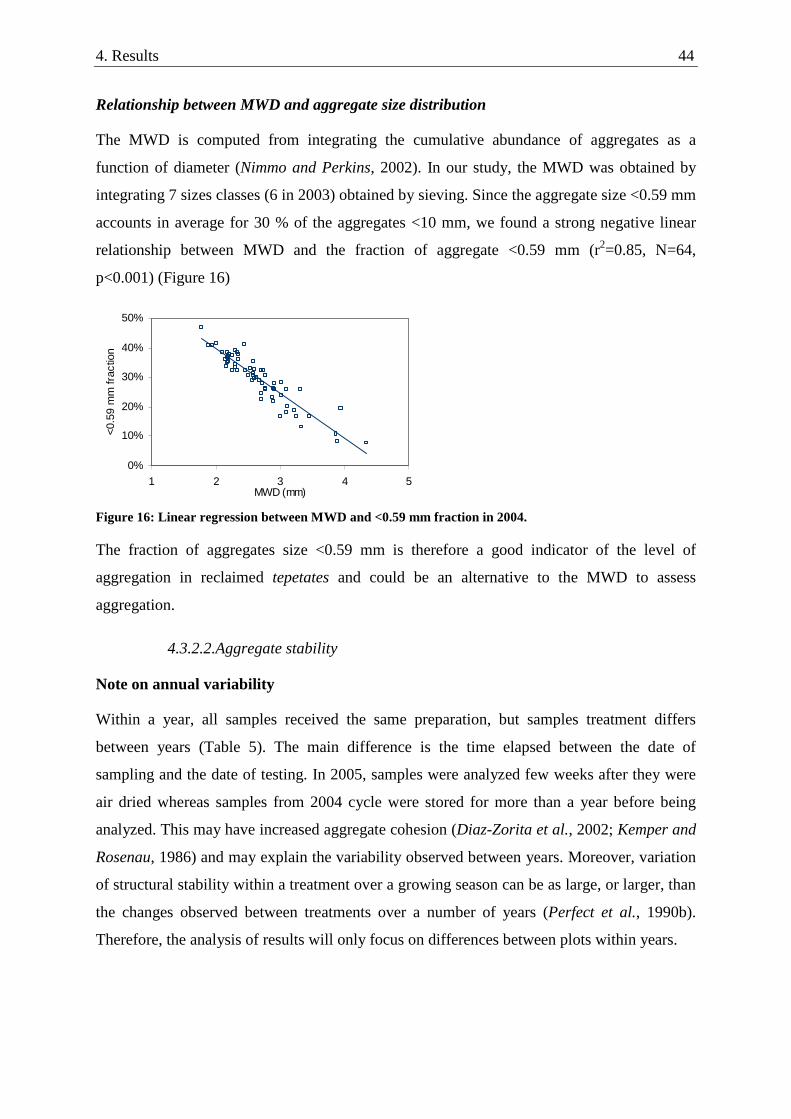
4. Results 44
Relationship between MWD and aggregate size distribution
The MWD is computed from integrating the cumulative abundance of aggregates as a
function of diameter (Nimmo and Perkins, 2002). In our study, the MWD was obtained by
integrating 7 sizes classes (6 in 2003) obtained by sieving. Since the aggregate size <0.59 mm
accounts in average for 30 % of the aggregates <10 mm, we found a strong negative linear
relationship between MWD and the fraction of aggregate <0.59 mm (r2=0.85, N=64,
p<0.001) (Figure 16)
0%
10%
20%
30%
40%
50%
1 2 3 4 5MWD (mm)
<0.5
9m
mfr
actio
n
Figure 16: Linear regression between MWD and <0.59 mm fraction in 2004.
The fraction of aggregates size <0.59 mm is therefore a good indicator of the level of
aggregation in reclaimed tepetates and could be an alternative to the MWD to assess
aggregation.
4.3.2.2.Aggregate stability
Note on annual variability
Within a year, all samples received the same preparation, but samples treatment differs
between years (Table 5). The main difference is the time elapsed between the date of
sampling and the date of testing. In 2005, samples were analyzed few weeks after they were
air dried whereas samples from 2004 cycle were stored for more than a year before being
analyzed. This may have increased aggregate cohesion (Diaz-Zorita et al., 2002; Kemper and
Rosenau, 1986) and may explain the variability observed between years. Moreover, variation
of structural stability within a treatment over a growing season can be as large, or larger, than
the changes observed between treatments over a number of years (Perfect et al., 1990b).
Therefore, the analysis of results will only focus on differences between plots within years.

4. Results 45
b
a
a
a
c
0
100
200
300
400
500
600
Conventional Improved Organic
PS
w
1986-plots
2002-plots
Figure 17: Effect of management and age of rehabilitation on mean PSw over the period 2003-2005.Different letter indicate significant difference (p<0.05).
On average over the period, there is a significant effect (p<0.001) of the age of rehabilitation
on PSw. 1986-plots were more stable to percolation (361.1 ml 10 min-1) than 2002-plots
(236.9 ml 10 min-1) (Table A- 17). Management also had a significant effect on PSw
(p<0.001), and this effect is not dependant from the year of rehabilitation (interaction not
significant). The effect of age of rehabilitation is clearly visible within a given management
(02-O significantly less stable than 86-O, and 02-C significantly less stable than 86-C)
(Figure 17). 02-O obtained similar PSw value (308.7 ml 10 min-1) than 86-C (259.3 ml 10
min-1) and 86-I (329.5 ml 10 min-1) (Table A- 17).
In 2005, aggregate stability was measured at three different dates during the rainfall season.
The results obtained illustrate the dynamic of aggregate stability in reclaimed tepetates
(Figure 18 and Table A- 17). The first sampling was done 2 months after compost was
applied in organic management (86-O and 02-O). We observed a peak of stability at the
beginning of the crop cycle with PSw values significantly greater in organic management
than in conventional and improved managements, regardless of the age of rehabilitation
(Table A- 17). PSw decreased in all plots at the end of the cropping season, and was
significantly lower in 2002-plots than in 1986-plots, both in conventional and organic
management.

4. Results 46
0
50
100
150
200
86-C 86-I 86-O 02-C 02-O
PS
w
13/07/05
22/09/05
17/11/05
Figure 18: Aggregate stability (PSw) in 2005 and its evolution during the crop cycle.
Detailed PS values for each aggregate size helps us analyze a step further the dynamic of
aggregate stability in reclaimed tepetates. For illustration sake, Figure 19 only show PS
values in 2002 plots for the 3 aggregate sizes tested. The results of all plots are presented in
Table A- 18.
0
100
200
300
13/07/2005 22/09/2005 17/11/2005 13/07/2005 22/09/2005 17/11/2005
02-C 02-O
PS
(ml
10
min
-1)
0.59 - 1 mm
1 - 2 mm
2 - 3.15 mm
Figure 19: PS (ml 10 min-1) values in 02-C and 02-O during the cropping season in 2005 in relation toaggregate size.
Since the PS index is the amount of water percolated through a column of calibrated
aggregates, we expect the PS index to be positively correlated to the aggregate size. Indeed,
in the hypothetical case of aggregates being uniform stable spheres, and assuming aggregates
are packed under the same model (Hillel, 2004), the smaller the aggregate diameter, the
smaller the resulting pores diameter, and in turn, the smaller the discharge.

4. Results 47
Figure 14 shows three mains features:
1. In recently reclaimed tepetate under conventional management (02-C) all aggregates
sizes had similar PS index (non significant differences).
2. In organic management (02-O), PS index for 2-3.15 mm aggregates was significantly
(p<0.01) higher than the other aggregate sizes on 13/07/05, but decreased and became
no longer significantly different after this date.
3. The stability of aggregates decreased during the growing season in all aggregate sizes.
At the end of the season, there were no differences in PS between managements.
In plots reclaimed in 1986, the same “stability peak” is observed in aggregates 2-3.15 mm at
the beginning of the cropping season in 86-O (332 ml 10 min-1) and, to a lesser extent, in 86-I
(208 ml 10 min-1) and 86-C (158 ml 10 min-1) (Table A- 18). PS values for aggregates 2 -
3.15 mm decreased during the season, but remained higher than smaller aggregates fractions
in all 86-plots.
Effect of ridge and furrow on aggregate stability
Traditionally in Mexico, maize is cultivated in a ridge and furrow system. In 2004, samples
were taken in ridge and furrow areas to evaluate the impact of such system on soil erodibility
(Table A- 17).
The furrow areas provided significantly higher PSw values (232 ml percolated in 10 min)
than the ridge area (139 ml 10 min-1). This is due to higher PS values for all 3 sizes of
aggregates, and not to a different aggregate size distribution (Table A- 18). This observation
suggests that a furrow-ridge system improves the overall aggregate stability thanks to the area
occupied by furrows. We assume that as runoff occurs in furrows, the particles are
transported according to their size and to the flow velocity, as shown in the Hjulström
diagram. When flow rate decreases, bigger particles settle whereas smaller particles are
transported downstream. This sedimentation process occurs in furrows and may result in a
coarser texture in these areas. As the sand fraction increases, the PS values obtained increase
too, since the PS is much positively correlated to the amount of sand in soils (Mbagwu and
Auerswald, 1999). In this case, higher PS values do not necessarily reflect higher cohesive
strength within the aggregate, but a higher porosity due to the amount a sands.
This hypothesis must be confirmed by PSD analysis in furrows and ridges areas.

4. Results 48
4.3.3. Porosity and pore size distribution
4.3.3.1.Total porosity and bulk density
Some definitions:
In our study, “fine pores” are the pores with equivalent diameter of less than 0.2 μm.
The volume of fine pores corresponds to the volume of water in the soil at 15 bars,
which is considered to be the physical definition of the permanent wilting point (θpwp)
“Large pores” are the pores with equivalent diameter of more than 10 μm. The
volume of large pores equals the volume of water in soil between field saturation and
field capacity (θfc) at -0.33 bar.
“Medium pores” are the pores whose equivalent diameter range from 0.2 to 10 m.
The volume of medium pores corresponds to the available water content, and is
equivalent to the volume of water retained in soil between θfc and θpwp.
Table 12: Mean porosity (0 – 40 cm) in reclaimed tepetates from 2003 to 2005 in Tlalpan. Different letterindicates significant difference (p<0.01)
Year ParameterMean Mean
2003 Pores >10 μm 11.3 a 11.8 a 12.8 a 12.0 12.7 a 10.2 a 11.4Pores 0.2 -10 μm 12.3 a 12.7 a 13.4 a 12.8 12.5 a 12.8 a 12.7Pores <0.2 μm 20.1 ab 20.3 ab 19.4 a 19.9 20.8 bc 21.7 c 21.3PT sat 43.6 a 44.8 ab 45.5 b 44.6 46.1 b 44.6 ab 45.3Bulk density 1.27 a 1.26 ab 1.23 ab 1.25 1.21 b 1.24 ab 1.22
2004 Pores >10 μm 16.5 a 17.1 a 16.0 a 16.5 14.8 a 17.1 a 15.9Pores 0.2 -10 μm 15.6 a 15.2 ab 14.9 ab 15.2 15.2 ab 13.8 b 14.5Pores <0.2 μm 16.0 a 15.2 b 15.3 b 15.5 17.6 c 18.6 d 18.1PT sat 48.0 bc 47.5 ab 46.1 a 47.2 47.5 ab 49.6 c 48.5Bulk density 1.22 a 1.19 ab 1.23 a 1.21 1.19 ab 1.16 b 1.18
2005 Pores >10 μm 20.1 ab 22.5 a 18.2 b 20.3 18.9 ab 20.1 ab 19.5Pores 0.2 -10 μm 13.9 a 13.2 a 15.8 b 14.3 14.3 ab 13.6 a 14.0Pores <0.2 μm 15.8 a 15.5 ab 15.0 b 15.4 17.6 c 18.6 d 18.1PT sat 49.8 ab 51.2 ab 49.0 a 50.0 50.8 ab 52.4 b 51.6Bulk density 1.16 ab 1.15 ab 1.19 a 1.16 1.15 ab 1.13 b 1.14
1986 2002Conventional Improved Organic Conventional Organic
In 2003 the bulk density ranged from 1.21 (02-C) to 1.27 g cm-3 (86-C), with an average of
1.24 g cm-3. Total porosity ranged accordingly from 43.6 to 46.1 % with an average of 44.9
%. Fine pores (<0.2 µm) represented in average 20.4 % of the soil volume and 45 % of the
total porosity. Large pores only accounted in average for 11.7 % of the soil volume.
In 2004, the average total porosity increased to 47.8 %, thanks to an increase in medium (14.9
%) and large pores (16.3 %). Fine pores decreased to 16.5 %. The difference between 2003
and 2004 is observed in all treatment, regardless of age or management. However, although

4. Results 49
large pores volume is not significantly different (p<0.05) between plots, fine pores volume is
significantly greater in recently reclaimed tepetates, both in 2004 and 2005.
In 2005, the average porosity increased to 50.6 % thanks to an increase in large pores (20 %).
The volume of medium and fine pores remained constant compared to 2004, at 14.1% and
16.5 % respectively. The same way as in 2004, the increase in porosity is observed in all
treatment regardless of age or management.
The increase in porosity between years is probably due to different soil conditions during
sampling rather than evolution of physical parameter over the years.
4.3.3.2.Pore size distribution
Detailed pore size distribution results are presented in Table A- 19, Table A- 20, and Table
A- 21.
In agreement with total porosity results, there is no significant difference in pore size
distribution between plots within a year (repeated measures ANOVA).

4. Results 50
Figure 20: Pore size distribution in 2003, 2004 and 2005 (Table A-19, A-20 and A-21)
4.3.3.3.Effect of depth on porosity
In 2003, total porosity ranged on average from 44.1 % at 10 cm depth to 45.2 % at 40 cm,
with no significant difference (P>0.05) between depth, regardless of the plot (Table A- 19
and Table A- 21)
In 2004, in ridge areas, the porosity varied on average between 48.6 % at 5 cm and 46.8 % at
40 cm, but this difference was not significant (Table A- 20).
In 2005, total porosity significantly decreased with depth, with values of 51.2 % in the first
20 cm depth, 49.5 % at 30 cm depth and 46.4 % at 40 cm. Porosity decreased with depth in
all plots (table A-17 appendix 6). The decrease in total porosity in linked to a decrease of the
volume of pores >10 µm, from 22.8 % at 10 cm depth to 14.4 % at 40 cm depth. The volume
of pores <10 µm remained constant in the profile with values ranging from 15.4 % at 5 cm

4. Results 51
and 15.2 % at 40 cm for medium pores and from 15.7 % at 5 cm to 16.8 % at 40 cm depth for
fine pores (Figure 21). The presence of structural crust and compaction of the upper horizon
is also clearly visible, with a decrease of larger pores (>120 µm) at 5 cm (3.3 %) compared to
10 cm (5.5 %) (Table A- 20).
-50
-40
-30
-20
-10
0
0 5 10 15 20 25
% of soil volume
Dep
th(c
m)
Large pores
Medium pores
Fine pores
Figure 21: Effect of depth on pore size distribution in 2005 in Tlalpan (Table A-21)
4.3.3.4.Effect of ridge and furrow systems on porosity
In 2004, maize was cultivated on a traditional ridge and furrow system. Samples were taken
both on furrow and ridge areas to assess the possible effect of such system on porosity.
Analysis of variance showed that in the first 5 cm depth, porosity in ridge area (48.6 %) is
significantly higher (p<0.001) than in furrow area (45.6 %), regardless of the plot (Figure 22).
0.0
4.0
8.0
12.0
16.0
<0.2 μm 0.2 - 3 μm 3 - 10 μm 10 - 30 μm 30 - 50 μm 50 - 120 μm >120μm
Pore size
%ofsoil
volu
me
Ridge
Furrow
Figure 22: Pore size distribution at 5 cm depth in ridge and furrow maize cropping in reclaimed tepetate(Table A- 22).

4. Results 52
The reduced porosity in furrows is due to a reduction of pores 50 -120 m and > 120 m. The
latter (> 120 m) occupy 7.1 % in ridge area against only 3.5 % in furrows. Volume of pores
<50 m is not significantly different between the two areas.
In furrows, runoff crusts are formed by successive organized deposits of sand and silt
particles settling down according to the flow velocity (Casenave and Valentin, 1989; Janeau
et al., 1992). The organization of particles and the absence of roots in this area reduced
macroporosity (> 50 m).
4.4. Statistical analysis
4.4.1. Relationship between SOC, aggregate stability and erodibility
Table 13: Bivariate covariance table between SOC, PS 1-2 mm (Percolation stability index measured onaggregates 1-2mm), PSw (weighted percolation stability index), MWD, runoff and soil loss (annualvalues) in reclaimed terraced tepetates.
SOC PS (1-2 mm) MWD PSw Runoff
2003 PS (1-2 mm) 0.62 -
MWD 0.74* 0.29 -
PSw 0.72* 0.85** 0.44 -
Runoff -0.96* -0.51 -0.57 -0.74 -
Soil loss -0.95* -0.47 -0.57 -0.69 0.98**
2004 PS (1-2 mm) 0.46 -
MWD 0.45 0.09 -
PSw 0.49 0.99** 0.19 -
Runoff -0.88* -0.34 0.14 -0.34 -
Soil loss -0.89* -0.36 0.12 -0.35 0.99**
2005 PS (1-2 mm) 0.78 -
MWD 0.50 -0.02 -
PSw 0.92* 0.97** 0.17 -
Runoff -0.95* -0.67 -0.42 -0.83 -
Soil loss -0.96** -0.73 -0.44 -0.87 0.98**
all years PS (1-2 mm) 0.39 -
MWD 0.33 -0.24 -
PSw 0.46* 0.98** -0.17 -
Runoff -0.89** -0.03 -0.22 -0.05 -
Soil loss -0.82** 0.01 -0.04 -0.01 0.93**
*. Correlation is significant at the 0.05 level (2-tailed).
**. Correlation is significant at the 0.01 level (2-tailed).
4.4.1.1.Relationship between aggregation and SOC content
Overall, the relationship between aggregation (PS, PSw, MWD) and SOC is very poor or
inexistent: there is no significant relationship between SOC and PS (1-2 mm), neither
between SOC and MWD (r= 0.33), and a weak, although significant (r=0.46), relationship
between SOC and PSw.

4. Results 53
The samples used for SOC analysis and the samples used for aggregation analysis (MWD,
PS, PSw) are different and were not taken at the same date. Therefore, SOC and aggregation
are related to the same plot, but not to the same sample. The lack of correlation is therefore
partly due a methodological problem and does not necessarily imply they are not related. This
result is discussed further in part 5.
4.4.1.2.Relationship between aggregation and erodibility
There is no significant relationship between the aggregation parameters (PSw, PS, MWD)
and erodibility (soil loss and runoff). Part of it can be attributed to methodological issues
already mentioned in part 4.3.2.
4.4.1.3.Relationship between SOC and erodibility
There is a strong relationship between SOC and soil erosion, for both soil loss (r = 0.82) and
runoff (r = 0.89). This relationship is analyzed further in the following chapter (4.4.2)
4.4.2. Soil loss and runoff prediction
The objective of this chapter is to:
1. Assess the relationship between erosivity, SOC and vegetation cover on soil loss and
runoff.
2. Predict soil loss and runoff in terraced reclaimed tepetates for individual event and
annual value
4.4.2.1. Data set
In total over the 3 years, 310 erosive events were recorded in the 5 experimental plots. Some
events were discarded according to the following criteria:
When detailed rainstorm data was not available
When runoff volume was below a threshold value of 1 mm in plots reclaimed in 1986,
or 5 mm in plots reclaimed in 2002. In cases where runoff was >1 mm in at least 2
plots (1986-plots), the event was included for all plots. This criteria was set to avoid
over representation of small events.
In total 141 events (or cases) were selected (Table A- 10). According to Tabachnick and
Fidell (2001), the minimum size recommended in a multiple regression is N> 50 + 8m where
m is the number of independent variables. In our study 3 independent variables are used. The

4. Results 54
number of cases selected if therefore approximately twice the minimum size recommended
(74). The model includes 45 % of the erosive events, and covers 77 % of the total soil loss
recorded. Descriptive statistics of the variables (Table A- 11) showed that soil loss, runoff,
and all the rain parameters are positively skewed. To comply with multivariate analysis
assumption of normality, skewed variables were logarithmically transformed.
4.4.2.2.Variables
SOC content
Since SOC content was not monitored throughout the cropping season but only at the end of
the season, annual values are used.
Vegetation cover prediction
Since vegetation cover was not monitored on a daily basis, we used predicted values of
vegetation cover for each erosive event in the analysis.
When the maximum value is known, vegetative growth pattern are well described by
symmetrical logistic equations (Landsberg, 1977), such as:
)exp(1
max
kTb
CCv
(10)
Where: Cv is the vegetation cover,
Cmax is the asymptote (maximum vegetation cover)
b and k are curvature parameters
T is time in days after planting.
In 2003 and 2005, b and k were determined to best-fit the measured data. In 2004, they were
set so that maximum vegetation cover was reached approximately 90 days after sowing.
After maximum crop development, leaf senescence causes vegetation cover to decrease. The
decay in vegetation cover was predicted by linear interpolation in 2003 and 2005. In 2004,
the decrease was considered to follow the same logistic curve after maximum value was
reached (90 days), with a loss of vegetation cover of 40% of the maximum value (Lizaso et
al., 2003).
Table 14: Curvature parameters for the modelling of vegetation cover . (a) Observed vs predicted.

4. Results 55
Year b k r2 (a) N Sig.2003 6 0.2 0.85 15 p<0.0012004 6 0.122005 9 0.2 0.94 58 p<0.001
4.4.2.3.Relationship between erosivity and erosion
EI30 is the rain erosivity parameter (R factor) used in the USLE (Wischmeier and Smith,
1978). It is the product of the kinetic energy of the storm with the maximum intensity in 30
minutes. Some authors (Prat, 1997) suggested that due to the rainstorm intensity patterns in
Mexican central highlands, EI10 should be better correlated to soil loss. Our results showed
that, in cultivated conditions, and for single events, EI10 is more strongly correlated with soil
loss than EI30, with average correlation coefficient of 0.55 and 0.52 respectively (Table A-
12). EI30 is however more strongly correlated to runoff than EI10, with r = 0.77 and 0.75
respectively. Rain precipitation and kinetic energy are also strongly related to runoff, with r =
0.77 and 0.78 respectively (Table A- 12). When detailed rainfall recording is not available,
rain depth can be used satisfactorily to predict runoff.
4.4.2.4.Soil loss and runoff prediction
For single event
Erosivity, Vegetation cover and SOC made a significant unique contribution to predict soil
loss and runoff. EI10 or EI30 are the best erosivity parameters to predict soil loss, explaining
together with vegetation cover and SOC 62 % of the variance (Table A- 13). Although not as
accurate as EI30 or EI10, rain depth is significantly correlated to soil erosion and can also be
used to predict soil loss instead of EI30 when detailed rainfall records are not available
(pluviometers).
The erosivity factor (EI30) made the greatest contribution to predict soil loss, accounting for
27 % (EI30) of the variance, whereas vegetation cover accounted for 26 % and SOC for
another 9 % (EI30) (Table A- 13).
Runoff was better predicted than soil loss thanks to a greater contribution of the erosivity
parameter. Both EI30 and rain depth, together with soil cover and SOC predicted
significantly (R2=0.68) the volume of runoff. EI30 alone accounted for 41 % of the total
variance, with soil cover contributing another 23 % and SOC only 4 %. Whereas EI10 is a
good indicator to predict soil loss, it is not so efficient to predict runoff (R2 = 0.64). EI30 is
the best erosivity indicator to predict both soil loss and runoff (Table A- 13).

4. Results 56
Finally, if runoff measurement are available, soil loss can be predicted with precision (R2 =
0.81). In this case runoff accounted for 68% of the variance and soil cover for another 13 %.
SOC did not make any significant unique contribution (P > 0.05) and was discarded.
Table 15: Multiple regression equation for single event soil loss and runoff prediction in terraced (slope 3-4%) cultivated tepetates in Tlalpan, Tlaxcala. Erosion (soil loss in kg ha-1); Runoff (mm); EI30 (MJ ha-1
mm h-1, or 10 N h-1); COVER (m2 m-2 :area of soil covered per unit of area); SOC (mg g-1).
Regression equation R2 Sig.
LOGerosion = 1.958 + 0.66(LOGEI30) - 1.09(COVER) - 0.15(SOC) 0.62 p<0.001
LOGrunoff = 0.046 + 0.62(LOGEI30) - 0.3(COVER) - 0.16(SOC) 0.68 p<0.001
LOGerosion = 1.96 + 1.05(LOGrunoff) - 0.76(COVER) 0.81 p<0.001
Soil loss and runoff prediction equations presented in table 9 are valid for individual erosive
events included in the range of those considered in the model and for terraced cultivated
tepetates with slopes of approximately 3 – 4 %, and with SOC content ranginf from 1 to 5 mg
g-1. They have not been validated for other conditions and should therefore not been
extrapolated.
The multiple regression analysis clearly highlighted that among the parameter that can be
influenced by management (vegetation cover and SOC), soil protection by vegetation cover
has the greatest impact on soil erosion. SOC also make a significant contribution to soil
erosion but to a lesser extent.
In case of a single extreme annual event (on average 45 mm and EI30 = 63 N h-1), and a
vegetation cover of 50 %, increasing SOC from 1 to 2 mg g-1 can reduce soil loss from 1.26 t
ha-1 to 0.88 t ha-1 (30 % decrease). For the same extreme annual event, and in reclaimed
tepetate with 1 mg g-1 SOC content, increasing vegetation cover from 50 to 80 % can reduce
soil loss from 1.26 t ha-1 to 0.59 t ha-1 (53 % decrease).
For annual values
The prediction models adjusted to annual runoff and soil loss explain a larger proportion of
the variances than for individual events (results in Table A- 14).
Annual runoff rates can be predicted by SOC and EI30 and COVER with good accuracy (r2 =
0.91, n = 15, Table 11). SOC alone is the main contributor and accounted for 79% of the
variance. Vegetation cover (COVER) and rain erosivity (EI30) explained another 6 % and 5
% of the variance respectively (Table A- 14).

4. Results 57
Erosion rates are well predicted by SOC content and EI30 (r2 = 0.84, n = 15, Table 11). In
that case SOC is the main contributor to soil loss variance (r2 = 0.64), whereas EI30 explained
another 20 %. Vegetation cover did not make any significant contribution to soil loss
prediction. When annual runoff data are available, 89 % of the annual soil loss can be
predicted. In this case runoff is the main contributor (r2 = 0.85), with EI30 accounting for
another 4 %. SOC and vegetation cover did not improve the model any further in this case
(no significant single contribution). Using the sum of EI30 of all erosive events only instead
of the annual EI30 (the sum of all events, both erosive and non-erosive) did not improve the
model fit.
Table 16: Multiple regression equation for annual soil loss and runoff prediction in terraced (slope 3-4%)cultivated tepetates. Soil loss (t ha-1); Runoff (mm); EI30 (N h-1); SOC (mg g-1); COVERmax (m2 m-2:vegetation cover at crop maximum development).
Regression equation r2 n Sig.
0.84 15 p<0.001
0.89 15 p<0.001
0.91 15 p<0.001Runoff = 256.23 - 37.50(SOC) + -144.82(COVERmax) + 0.207(EI30)
Soil loss = 9.75 - 3.98(SOC) + 0.03(EI30)
Soil loss = 0.07(RUNOFF) + 0.015(EI30) - 4.83
The significance of the regression analysis greatly depends on the contrast between 86-plots
and 02-plots. There is a strong relationship between runoff rates and SOC in recently
reclaimed plots, but no relationship in 86-plots (figure 11).
0
100
200
300
0 1 2 3 4 5
SOC (mg g-1)
Runoff
(mm
)
1986-plots
2002-plots
Figure 23: Relationship between SOC and annual runoff rates in plots reclaimed in 1986 and 2002.
It is important to stress that annual sediment and runoff rates prediction are based upon 15
values (5 plots * 3 years), and although the r2 reported are adjusted to take into account the

4. Results 58
size of the sample, the latter is under the recommended size. All interpretation based upon the
regression equations proposed should be made with the necessary critical judgment.

5. Discussion: Effect of organic farming on soil erosion and soil structure 59
5. Discussion: Effect of organic farming on soil erosion and soil structure
5.1. Erosivity
Rain erosivity in Tlalpan is moderate, with average annual precipitation of 675 mm and
average R of 127 N h-1. It is however, higher than on the western side of the Sierra Nevada
(Prat, 1997).
Our results complement the previous studies of Baumann (1996) and Fechter-Escamilla
(1997a) and give a longer term perspective of rainfall patterns in the Bloque de Tlaxcala.
Rainfall patterns recorded over the 2002-2005 period and confirmed that in this region soil
loss is caused by a reduced number of rainstorms. Such rainfall and erosion distribution
pattern have also been observed in many locations in the world and under contrasting rainfall
regime (Edwards and Owens, 1991; Langdale et al., 1992; Nyssen et al., 2005; Gonzalez-
Hidalgo et al., 2007).
Rain erosivity in Tlalpan have been extensively discussed by Baumann (1996). Our results
confirm trends previously reported but do not give further insights. Hence, this aspect won’t
be developed further.
5.2. Effect of organic farming on soil erosion
5.2.1. Carbon dynamic in reclaimed tepetates
5.2.1.1.Incorporation and accumulation of SOC
In organic management, organic fertilization was applied at an average rate of 3.7 and 4.1 t
ha-1 yr-1 (dry material) in 86-O and 02-O respectively. Such rates are lower than organic
fertilization rates applied in other experiments in reclaimed volcanic ash soils:
i. In Eastern side of the Sierra Nevada, Baez et al. (1997) applied 40 t ha-1 fresh farmyard
manure the first year after fragmentation and 20 t ha-1 the years onwards.
ii. In Ecuadorian Cangahua, Podwojewski and Germain (2005) applied 40 t ha-1 dry material
after fragmentation and 10 t ha-1 the following years.
iii. Acebedo et al. (2001) studied tepetate aggregation in greenhouse conditions after
incorporation of the equivalent of 50 t ha-1 dry cattle manure.

5. Discussion: Effect of organic farming on soil erosion and soil structure 60
iv. In Salvador, Collinet and Mazariego (1993) used 15 t ha-1 yr-1 dry poultry manure to
reclaim volcanic ash soils.
Manure or compost application of more than 10 t ha-1 yr-1 are hardly available for the average
farm in the area (Lepigeon, 1994) and would require external provision of organic material
(manure, residues, etc..). It would in turn increase production costs and make the farm more
dependant on external inputs. The organic management evaluated in our experiment was
designed to be acceptable and adoptable by local small holders, as well as being
economically viable and environmentally reproducible. Ideally, organic farming should limit
external inputs to reduce costs and tend to be self sufficient in terms of organic fertilization.
In this respect, compost should be produced using the amount of residues available from the
previous crop and manure produced on the farm. For experimentation sake, it was not
possible to follow this principle every year, but attempt has been made to keep external inputs
of organic material to reasonable levels and to make the organic management reproducible
and adoptable to small farmers in the area.
In plots reclaimed in 1986, 20 % (on average) of the C incorporated between 2002 and 2005
was accumulated in soil (Table 8). In recently reclaimed tepetates this ratio was 24 % in
organic management and 40 % in traditional management. The higher translocation
efficiency in traditional management can be explained by the origin of the C incorporated.
Numerous studies have demonstrated that root-derived Carbon was more persistent than
shoot-derived C (Rasse et al., 2005). Puget and Drinkwater (2001) observed an increased
retention of root-derived C in soils 6 months following crop incorporation in comparison to
shoot-derived C. Experimental results summarized by Bolinder et al. (1999) also suggest that
the percentage of below ground corn-C incorporated into SOC (range 16 – 30 %) is higher
than that from above ground corn biomass (range 7.7 – 20 %). Hence, since the percentage of
C inputs from roots is higher in 02-C than in the other plots, a greater proportion of C
incorporated was accumulated in the soil in comparison to other systems. Our results are
coherent with those reported by Bolinder, although differences exist because our study
considered C translocation from different crops (not only maize) without discrimination
between above- and below-ground C inputs.
On irrigated intensive cropping Vertisols in Central Mexico, Follett et al. (2005) calculated C
sequestration efficiency of 22 % for above-ground C and estimated to 11 % the C
sequestration efficiency for total C incorporated (above- and below-ground C).
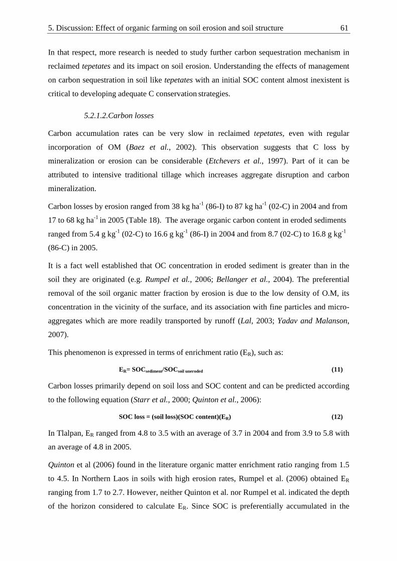
5. Discussion: Effect of organic farming on soil erosion and soil structure 61
In that respect, more research is needed to study further carbon sequestration mechanism in
reclaimed tepetates and its impact on soil erosion. Understanding the effects of management
on carbon sequestration in soil like tepetates with an initial SOC content almost inexistent is
critical to developing adequate C conservation strategies.
5.2.1.2.Carbon losses
Carbon accumulation rates can be very slow in reclaimed tepetates, even with regular
incorporation of OM (Baez et al., 2002). This observation suggests that C loss by
mineralization or erosion can be considerable (Etchevers et al., 1997). Part of it can be
attributed to intensive traditional tillage which increases aggregate disruption and carbon
mineralization.
Carbon losses by erosion ranged from 38 kg ha-1 (86-I) to 87 kg ha-1 (02-C) in 2004 and from
17 to 68 kg ha-1 in 2005 (Table 18). The average organic carbon content in eroded sediments
ranged from 5.4 g kg-1 (02-C) to 16.6 g kg-1 (86-I) in 2004 and from 8.7 (02-C) to 16.8 g kg-1
(86-C) in 2005.
It is a fact well established that OC concentration in eroded sediment is greater than in the
soil they are originated (e.g. Rumpel et al., 2006; Bellanger et al., 2004). The preferential
removal of the soil organic matter fraction by erosion is due to the low density of O.M, its
concentration in the vicinity of the surface, and its association with fine particles and micro-
aggregates which are more readily transported by runoff (Lal, 2003; Yadav and Malanson,
2007).
This phenomenon is expressed in terms of enrichment ratio (ER), such as:
ER= SOCsediment/SOCsoil uneroded (11)
Carbon losses primarily depend on soil loss and SOC content and can be predicted according
to the following equation (Starr et al., 2000; Quinton et al., 2006):
SOC loss = (soil loss)(SOC content)(ER) (12)
In Tlalpan, ER ranged from 4.8 to 3.5 with an average of 3.7 in 2004 and from 3.9 to 5.8 with
an average of 4.8 in 2005.
Quinton et al (2006) found in the literature organic matter enrichment ratio ranging from 1.5
to 4.5. In Northern Laos in soils with high erosion rates, Rumpel et al. (2006) obtained ER
ranging from 1.7 to 2.7. However, neither Quinton et al. nor Rumpel et al. indicated the depth
of the horizon considered to calculate ER. Since SOC is preferentially accumulated in the

5. Discussion: Effect of organic farming on soil erosion and soil structure 62
upper layers of the soil, ER can be greatly influenced by the depth of the horizon considered
in the calculation. In the UK, Owens (2002) found ER of 1.2 to 1.5 in average and concluded
that it was easier to apply techniques to reduce erosion rates, and thereby carbon losses than
applying techniques to reduce ER. Even though ER comparisons with other studies found in
the international literature are hazardous because of the lack of information regarding the
depth of the horizon that was considered to calculate ER, it appears that our values of ER are
higher than the one reported in template regions. This is likely to be due to the very low SOC
content in reclaimed tepetates which increase the contrast between the arable horizon and the
upper part of the horizon where SOM is concentrated.
Table 17: Carbon losses by erosion and C concentration in sediment in Tlalpan in 2004 and 2005. Source:(Báez et al., 2006).
86-I 86-O 86-C 02-C 02-O
C losses by erosion (kg C ha-1) 2004 38 65 71 87 852005 17 22 22 75 68
C in sediment (g C kg-1) 2004 16.6 15.3 12.7 5.4 8.32005 15.7 15.8 16.8 8.7 12.4
C lost / C accumulated 2004 0.10 0.11 0.34 0.40 0.112005 0.05 0.04 0.11 0.35 0.08
ER (SOC at 0-10 cm) 2004 4.8 3.4 3.3 3.6 3.5
2005 4.7 3.9 4.6 5.8 5.2
In 2005, C losses by erosion represented approximately 10% of the average C accumulation
rate in Organic and Improved management. However in conventional management, where C
inputs are limited, C losses by erosion represented 34 % (86-C) and 40 % (02-C) of the C
accumulated per year. Losses of carbon by erosion in reclaimed tepetates are significant but
are easily balanced by organic matter inputs from roots and crop residues, even in traditional
management. Soil erosion is thus a phenomenon which does not cause severe on-site
depletion of carbon content as reported in other ecosystems (Lal, 2003), but which reduces C
accumulation rate in cultivated tepetates.
Baez et al. (2006) and Covaleda et al. (2007) concluded that carbon losses by erosion in
reclaimed tepetates were minimal in the carbon balance and that loss of C occurred almost
exclusively by mineralization. Nonetheless, although on-site losses of carbon in reclaimed
tepetates are limited, the mechanisms involved in soil erosion greatly contribute to carbon
losses. Aggregate breakdown by slaking, differential swelling, or raindrop impact (Le
Bissonnais, 1996) releases encapsulated carbon which is then exposed to oxidation and
microbial processes (Six et al., 2004). In addition, the C released is preferentially transported
by runoff or wind (Lal, 2003). Whereas on-site removal of SOM by erosion can be

5. Discussion: Effect of organic farming on soil erosion and soil structure 63
redistributed within the watershed or ecosystem, SOM exposed to mineralization or oxidation
by breakdown of aggregate is lost to the atmosphere (Polyakov and Lal, 2004). More research
is needed to determine the part of carbon mineralization induced by the mechanism involved
in soil erosion, and the effect of organic farming on C mineralization.
5.2.2. Vegetation cover
Vegetation cover reduces particle detachment by intercepting and dissipating part of the
energy of raindrops before they strike the soil surface (Hudson, 1995). As a result, it reduces
sealing and crust formation, favours infiltration and, hence, decreases runoff and erosion rates
(Box and Bruce, 1995; Stocking, 1994; Morgan, 2005). There are numerous evidences of the
positive effect of vegetation cover on soil erosion in international literature. In chapter 4.4.2,
the regression analysis showed that vegetation cover explained 26 % of the variance in soil
loss for individual rainstorm. This result gives a quantitative indication of the effect of
vegetation cover in reclaimed tepetates, and the role this factor can play in the first years after
fragmentation.
The discussion will not focus on the effect of vegetation cover on soil erosion, which is a fact
very well established, but on the way management practices can affect vegetation cover. Two
aspects are considered: 1) crop development, which depends on plant nutrition and water
supply, and 2) crops association.
5.2.2.1.Crop development and vegetation cover
As presented before (Table A- 7) recently fragmented tepetates are almost sterile material
due to their lack of N and P, but these deficiencies can be overcome by appropriate
fertilization to reach acceptable crop production (Etchevers et al., 1992; Navaro and
Zebrowski, 1992; Marquez et al., 1992; Baez et al., 1997).
In practice, small-holders in the area tend to adapt the amount of fertilization to their financial
capacities at the time the fertilization is required. As a result, fertilization in traditional
management is often below crop requirements and can limit crop development and vegetation
cover. Our results clearly showed that in recently reclaimed tepetates, the amount of
fertilization applied under conventional management (02-C) don’t overcome fertility
deficiencies and result in poor vegetation cover.
When applied at 15 t ha-1 (fresh manure) in recently fragmented tepetates, organic
fertilization provided vegetation cover similar to tepetates cultivated for more than 15 years.

5. Discussion: Effect of organic farming on soil erosion and soil structure 64
However, in 2005 with wheat cropping, the amount of compost applied in 02-O (4.2 t ha-1)
resulted in poor crop development and vegetation cover. This observation suggests that the
amount of organic fertilization required to provide an optimum nutrition for the crop is
greater than what can be produced by composting the previous crop residues. Two options
can be considered to reach optimum crop development and vegetation cover:
1) Increasing the organic fertilization, with additional inputs of manure, produced on the
farm or purchased locally, or compost. The latter implies purchasing additional
organic material to be composted (straw, maize stalks, etc…). Further research is
needed to evaluate the cost-benefit relationship and the cost of opportunity of strict
organic farming.
2) Complementing organic fertilization with mineral fertilization, which is an effective
way to increase soil fertility (FAO, 1999).
In any cases, the fertilization strategy must be adapted to the type of production system found
in the area and to the specific conditions of the smallholders.
Water supply
Results of porosity showed no evidence of significant differences in water holding capacity
between plots (Chapter 4.3.3). However, surface crusting and sealing enhanced by aggregate
breakdown reduce infiltration and, as a consequence, water storage and availability for plants.
The frequent monitoring of soil water content done in 2005 indicated that over the period
2002-plots were significantly drier than 1986-plots (Table A- 9). This is consistent with
runoff measurements which showed that in 2005, 164 mm and 140 mm water were lost by
runoff in 02-C and 02-O respectively, against 33 mm on average in 86-plots (Table A- 2). It
clearly highlights that when nutrition deficiencies are not overcome, either by organic or
mineral fertilization, it gives rise to a vicious circle that will enhance soil erosion: nutrition
deficiencies reduce crop growth and vegetation cover. This will enhance surface crusting and
sealing and will increase runoff. In turn, water losses by runoff decrease water supply which
will affect plant growth and vegetation cover (Figure 24).
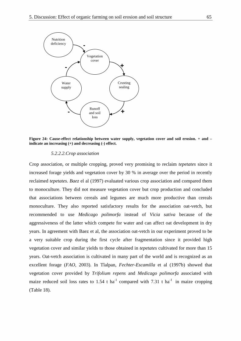
5. Discussion: Effect of organic farming on soil erosion and soil structure 65
Crustingsealing
Runoffand soil
loss
Watersupply
Nutritiondeficiency
Vegetationcover
+
+-
-
-
Figure 24: Cause-effect relationship between water supply, vegetation cover and soil erosion. + and –indicate an increasing (+) and decreasing (-) effect.
5.2.2.2.Crop association
Crop association, or multiple cropping, proved very promising to reclaim tepetates since it
increased forage yields and vegetation cover by 30 % in average over the period in recently
reclaimed tepetates. Baez el al (1997) evaluated various crop association and compared them
to monoculture. They did not measure vegetation cover but crop production and concluded
that associations between cereals and legumes are much more productive than cereals
monoculture. They also reported satisfactory results for the association oat-vetch, but
recommended to use Medicago polimorfa instead of Vicia sativa because of the
aggressiveness of the latter which compete for water and can affect oat development in dry
years. In agreement with Baez et al, the association oat-vetch in our experiment proved to be
a very suitable crop during the first cycle after fragmentation since it provided high
vegetation cover and similar yields to those obtained in tepetates cultivated for more than 15
years. Oat-vetch association is cultivated in many part of the world and is recognized as an
excellent forage (FAO, 2003). In Tlalpan, Fechter-Escamilla et al (1997b) showed that
vegetation cover provided by Trifolium repens and Medicago polimorfa associated with
maize reduced soil loss rates to 1.54 t ha-1 compared with 7.31 t ha-1 in maize cropping
(Table 18).

5. Discussion: Effect of organic farming on soil erosion and soil structure 66
5.2.2.3.Mulching
In Mexican highlands, like in semi arid areas, the extended dry season prevent the
establishment of cover crop before the onset of the rainfall season, leaving the soil exposed to
the first erosive rainstorms. Mulching is an alternative whose effectiveness is widely
recognized (e.g. Lal, 1995; Morgan, 2005; Hobbs, 2007). The residue cover both protects the
soil from raindrop impact and decreases stream power by increasing roughness.
Mulching has not been evaluated in Tlalpan within REVOLSO project, but has been
evaluated in Michoacan on reclaimed deteriorated Acrisols by Bravo et al. (2006). They
showed that 30 % residue cover by at the beginning of the rainfall season reduced erosion
rates by 70 % compared to unprotected soil. Similar results were obtained previously in
Patzcuaro watershed on andosols by Tiscareno-Lopez et al. (1999). More examples of soil
loss reduction by mulching in different type of soils and climate are given by Morgan (2005)
who suggest that an application of 5 t ha-1 of straw is sufficient to achieve an optimum soil
cover of 70 to 75 %. In Mexico, Roldan et al (2003) used approximately 3 t ha-1 crop residue
to provide 33 % ground cover, and approximately 5 t ha-1 to provide 66 % ground cover.
Mulching requires significant amount of residues, which will be incorporated to the soil and
mineralized. However in the study area, crop residues are traditionally exported for animal
pasture despite their poor nutrimental value. Residue management is, thus, an issue that must
be address since soil conservation practices that promote organic matter incorporation and
mulching are competing with traditional use of crop residues. To increase probabilities that
farmers adopt new technologies, it is therefore necessary to develop simultaneously
sustainable alternatives to traditional animal feeding system.
5.2.3. Runoff and erosion rates in reclaimed tepetates
After 16 years of cultivation, soil erosion rates in reclaimed terraced tepetates in Tlaxcala are
below 5 t ha-1 yr-1. Soil loss rates below 10 t ha-1 yr-1 are usually considered tolerable
(Hudson, 1995; Morgan, 2005). Soil erosion is critical after fragmentation, with soil loss
rates of more than 15 t ha-1 yr-1, but can be kept within acceptable range as long as they are
cultivated with dense vegetation cover within the first years of cultivation. The study proved
that regular incorporation of OM to the soil after fragmentation reduces significantly erosion
rates from the first years after fragmentation.
In Tlalpan, soil erosion has been measured previously at field scale in 1995 and 1996 in
tepetates cultivated for 9 and 10 years after fragmentation (Fechter-Escamilla et al., 1997b).

5. Discussion: Effect of organic farming on soil erosion and soil structure 67
The two years were little erosive, with R factor of 196 N h-1 and 218 N h-1 respectively, and
erosion rates ranged from 1.54 ton ha-1 to 7.31 ton ha-1 depending on the treatment (Table
18). Reduced tillage without soil cover increased significantly runoff rates because of the low
infiltration in the upper horizon (Fechter-Escamilla et al., 1997b), increasing in turn erosion
rates compared to traditional tillage. However, reduced tillage with additional ground cover
provided by the associated crops both reduced runoff and soil loss compared to traditional
tillage.
Table 18: Field scale (1200 – 1500 m2) soil loss and runoff in Tlalpan in 1995 and 1996. Source: Fechter-Escamilla et al. (1997b). LT: Traditional tillage (Maize cropping with soil preparation by disc ploughingand two hoeing during cropping); LRscv: No tillage without vegetation cover (Maize cropping by directsowing and weed control with herbicides); LRccv: No tillage with associated vegetation cover (Maizecropping with no tillage and association of Trofolium repens and Medicago polimorfa)
LT LRscv LRccv
1995 Soil loss (ton ha-1) 3.00 3.72 2.34Runoff (mm) 76 132 53Annual precipitation : 603 mm
EI30: 196 N h-1
1996 Soil loss (ton ha-1) 5.02 7.31 1.54Runoff (mm) 30 98 11.2Annual precipitation: 607 mm
EI30: 218 N h-1
On the Eastern hillside of the Sierra Nevada, Prat et al (1997a) carried out field scale (700
m2) erosion studies where they measured erosion rates in recently reclaimed tepetates under
managements similar to those we assessed in Tlalpan. In their experiment, the “monoculture”
system is equivalent to our traditional management, with use of mineral fertilizers and no
associated crop. Their system called “associated crop and O.M.” is similar to our organic
management, with application of 40 t ha-1 fresh manure in 2003 and 20 t ha-1 the following
years, and use of associated crops.
They found that in average, crop association and incorporation of organic matter reduced
erosion rates to 2 t ha-1 compared with 7.8 t ha-1 under monoculture system. However, they
obtained the same effect with crop association and mineral fertilization, suggesting that the
effect of vegetation cover prevails upon the effect of organic fertilization. The erosion rates
they reported are smaller than those we obtained in Tlalpan. This difference in mainly
explained by the fact that rainfall erosivity in San Miguel Tlaixpan (the name of the place
where their experimental site was located) over the period 1993-1996 was only 205 N h-1 on
average (Prat, 1997), whereas in Tlalpan over the period from 2003 to 2005, the R factor was
on average 305 N h-1. Besides this difference, our results are consistent with their conclusions

5. Discussion: Effect of organic farming on soil erosion and soil structure 68
that vegetation cover plays a major role in controlling erosion rates in the first years after
fragmentation.
5.2.4. Evolution of erosion rates
Our results clearly highlighted the high sensibility of recently fragmented tepetates to soil
erosion, with soil loss rates up to 3 times higher than in reclaimed tepetates cultivated for
more than 15 years. After such period of time, tepetates seem to have reached a stable level
below acceptable soil loss rates. Some uncertainties remain though as of how fast erosion
rates decrease and how many years are required before reclaimed tepetates can be considered
stables. This is a fundamental question to design and implement sustainable rehabilitation
programs.
In chapter 4.4.2, we showed that soil loss variance in reclaimed tepetates depends on
erosivity, SOC and vegetation cover. We thus expect the evolution of erosion rates to depend
on the evolution of these three parameters. Assuming that i) rainfall erosivity is a random
parameter, with independent behavior from one year to another; ii) vegetation cover is a
parameter that can be controlled by management practices (type of crop, fertilization) at each
cropping cycle; then over time, the evolution of erosion rates is linked to the evolution of
SOC content and, as a result, to C accumulation rates.
Yet, little is known about C accumulation in soils with initial SOC content almost inexistent
such as reclaimed tepetates. Most recent studies on C accumulation or sequestration rates in
agricultural lands deal with SOC variation after agricultural management changes (e.g.
review by Post and Kwon, 2000), such as change from conventional tillage (CT) to no tillage
(NT) (West and Post, 2002). The latter reported that when changing from CT to NT, it is
possible to sequester 0.57 ± 0.14 Mg C ha-1 yr-1, with SOC reaching a new equilibrium after
15 to 20 years. Lal et al. (1998; cited by FAO, 2004), quantified carbon sequestration
potential for different technological options in drylands. For compost application, they
suggested C sequestration rates of 0.10 to 0.20 Mg ha-1 yr-1, similar to C sequestration
potential for agriculture intensification or conservation tillage, but less than that of water
conservation and management (0.10 to 0.20 Mg ha-1 yr-1).
Baez et al. (2002) suggested that C accumulation in reclaimed tepetates followed a
logarithmic increase in time, regardless of the type of management. In the case of maize
monocropping, Baez et al. observed that SOC content tends to become stable after the first

5. Discussion: Effect of organic farming on soil erosion and soil structure 69
decade and argued that SOC content could hardly increased even after 50 or 100 years due to
the limited amount of organic matter incorporated in this type of agricultural management.
Our results showed that the fragmentation and the subsequent cultivation of tepetates induced
by itself a carbon sequestration process. Cultivation, even with low OM inputs such as the
conventional management, provided enough organic material (roots and harvest residues) to
sequester around 0.2 Mg C ha-1 yr-1 (02-C) in the top 20 cm soil. The same C sequestration
rate (0.2 Mg C ha-1 yr-1) was also measured 16 years after fragmentation (86-C). This
“baseline” C sequestration rate can be multiplied by 4, to 0.8 Mg C ha-1 yr-1 with additional
organic matter inputs in the years following fragmentation. The implementation of organic
farming after 16 years of conventional farming did increase SOC content and C sequestration
to 0.61 Mg C ha-1 yr-1. However, the SOC increase was not correlated to any significant
decrease in sediment rates. This observation suggests the existence of a threshold value of
approximately 3.4 mg g-1 at 0-10 cm (Figure 23) above which: i) SOC has no further effect
on soil erosion; or ii) differences in SOC are not large enough to produce significant
differences in runoff and erosion rates at field scale.
Assuming linear accumulation rates presented in table A-19 (0-10 cm) and the regression
model proposed in table 11:
i. Reclaimed tepetates could reach SOC content higher than 3.4 mg g-1 at 0-10 cm depth
(stability threshold) after 7 years of cultivation under organic management and after 21
years under conventional management.
ii. Assuming an average year (erosivity = 279 N h-1), erosion rates in reclaimed tepetates could
drop below tolerable rates (10 t ha-1) after 3 years under organic management and after 9
years under conventional management.
These estimations seem realistic for the organic management. For conventional management,
the mean accumulation rates observed over the first 4 years after fragmentation (0.09 mg g-1
yr-1) is lower than the estimated mean accumulation rates in plots reclaimed in 1986 over a
period of 16 years (0.15 mg g-1 yr-1). If we take into account this value instead of the one we
observed over a period of 4 years, tolerable erosion rates could be reach after 7 years instead
of 9 years and the stability threshold could be reach after 17 years instead of 21 years under
conventional management. In any cases, organic management after fragmentation can reduce
the critical period when reclaimed tepetates present high erodibility by 2 to 3 time compared
to conventional management.

5. Discussion: Effect of organic farming on soil erosion and soil structure 70
5.3. Effect of organic management on soil structure
5.3.1. Aggregate stability dynamic and organic management
Aggregate stability expresses the resistance of aggregates to breakdown when subjected to
potentially disruptive processes (Hillel, 2004). Aggregate stability is affected by soil texture,
clay mineralogy, organic matter, cations concentration, iron and aluminium oxides and
CaCO3 (Le Bissonnais, 1995). We will focus on the effect of organic matter since the primary
soil characteristics of the reclaimed tepetates we studied are similar, and because differences
between managements and age of rehabilitation are mainly based on soil organic carbon
content.
Organic matter enhances formation and stability of aggregates by bonding and/or holding
particles together (Oades, 1984). More recently, several studies have demonstrated that the
hydrophobicity of organic matter also greatly contributes to aggregate stability by decreasing
wettability of aggregates, reducing the magnitude of slaking and differential swelling (Chenu
et al., 2000; Goebel et al., 2005; Zaher et al., 2005).
The ANOVA of percolation stability test revealed a positive effect of age of rehabilitation
(2002-plots against 1986-plots) and of organic management on aggregate stability, regardless
of the age of reclamation. This observation (Figure 17) suggests that aggregate percolation
stability is the result of the combination of:
i. Time-driven stability that develops over the years during the rehabilitation process, and
which is related to SOC content
ii. Management-driven stability, independent from the age of rehabilitation, which is related
to the incorporation of fresh organic material (crop residues, compost or manure)
Results from 2005 (Figure 18, Table A- 17) complement this observation by showing that:
i. At the beginning of the rainfall season, a few weeks after incorporation of fresh organic
matter, we observed a peak of stability in organic management. 02-O obtained similar
percolation values than 86-C and 86-I, although SOC content in 02-O is lower than in 86-C
and 86-I. This observation indicates that the stability provided by the incorporation of fresh
organic matter (management driven stability) prevails upon the stability provided by SOC
content (time driven stability). It would also explain why SOC and PS are weakly related.
ii. At the end of the rainfall season, percolation stability in 2002-plots, both under
conventional and organic management, dropped below the percolation stability measured in

5. Discussion: Effect of organic farming on soil erosion and soil structure 71
1986-plots. This observation suggests that the effect of fresh organic matter incorporation
on percolation stability is short-lasting (3 to 4 months).
These results are coherent with several studies that showed that the stability of
macroaggregates is not related to SOC but to other organic compounds (Tisdall and Oades,
1982). Perfect and Kay (1990) found that increases in wet-aggregate stability did not
correlate with increases in total organic carbon content, suggesting that some components of
the organic carbon pool were more actively involved in stabilizing aggregates than others.
Golchin et al. (1995) concluded that neither total organic matter nor total O-alkyl Carbon
content was closely correlated with aggregate stability, and suggested that only a part of soil
carbon or carbohydrate was involved in aggregate stability. They also found that particulate
organic matter occluded within aggregates was better correlated with aggregate stability.
The peak of stability observed in organic management a few weeks after organic matter
inputs is coherent with contemporary models of aggregates formation and stabilization.
According to the model of aggregate formation proposed by Puget et al. (2000), when fresh
organic material from plants is incorporated into the soil matrix, it is rapidly colonized by
microbial decomposers. Fungal hyphae and other by-product of the microbial activity, such
as extra cellular polysaccharides, bind soil particles to the particulate OM. It refers to what
Tisdall and Oades (1982) had called “transient” binding agents, responsible for the
aggregation of macroaggregates (>250 µm). According to these authors, polysaccharides are
produced rapidly after addition of organic materials, and the effect of transient binding agents
on water stable aggregation can starts 2 to 3 weeks after the addition of organic materials,
depending on the nature of these materials. Watts et al. (2001) investigated how soil structure
responded when fresh organic materials were added to poor quality degraded arable soils and
concluded that the incorporation of dried grass leaves into degraded soil increased
aggregation and that the process of aggregation was microbiologically mediated. Plante and
McGill (2002) demonstrated the formation of macroaggregates by incorporation of tracers 9
days after tillage. They found that a maximum of 40 to 60 % tracers were incorporated into
>1-mm aggregates after 72 days. Using the same percolation stability test, Fechter-Escamilla
et al. (1997b) were able to show evidence of short term structural stability increase in the
upper horizon of reclaim tepetate induced by ground cover of Trifolium repens and Medicago
polimorfa. They attributed this observation to the increased microbial activity enhanced by
favourable soil moisture regime and roots development provided by the cover crops.

5. Discussion: Effect of organic farming on soil erosion and soil structure 72
The seasonal decrease of PS can be attributed to seasonal fluctuations of roots and microbial
biomass and/or level of organic stabilizing constituent (Perfect et al., 1990a). Indeed, even
though transient binding agents are produced rapidly after incorporation of OM, they are also
decomposed rapidly by microorganisms (e.g. Oades, 1993). In soils with low OM, the
macroaggregates breakdown resulting from raindrop impact during the rainfall season leads
to exposure and decomposition of the new and young OM enclosed in the macroaggregates
formed at the beginning of the growing season, after the incorporation of fresh organic matter
(Plante and McGill, 2002). As decomposition of the incorporated OM proceeds, the
microbial growth and production of biopolymers decrease, together with their aggregating
action. We think that aggregate breakdown by raindrop impact during the rainfall season may
expose the OM enclosed in macroaggregates, and accelerate its decomposition, resulting in a
rapid decrease of the aggregate stability.
The fact that at the end of the season (2005) PSw was higher in 1986-plots than in 2002-plots
showed that the stability related to SOC is more recalcitrant and long lasting than the stability
related to the incorporation of fresh organic matter.
Covaleda et al. (2007) conducted a more detailed analysis of carbon dynamic in reclaimed
tepetates in Tlalpan using fractionation techniques. They concluded that: i) the C
incorporated (manure, compost) is stored primarily in macroaggregates (>0.2 mm), this
aggregate-size fraction being the most sensitive to management practices; ii) in the medium
term, the C stored in the smallest aggregates (<0.05 mm) increased. These results are
coherent with the model of aggregate hierarchy (Tisdall and Oades, 1982; Oades and Waters,
1991) which proposed that micro-aggregates (<250 μm) are bound together into macro-
aggregates (>2000 μm) and stabilized by a network of roots and hyphae and by transient
binding agents such as microbial- and plant-derived polysaccharides. Oades (1984) later
showed that the formation of microaggregates occurs within macroaggregates and is
enhanced by the decomposition of temporary binding agents. This mechanism implies that
the SOC in microaggregates is more recalcitrant, whereas the SOC in macroaggregates more
labile (Degens, 1997). Puget et al. (1995) also demonstrated that the SOM responsible for the
stability of macroaggregates was younger than the one present in microaggregates. This
conceptual model has been confirmed by several studies (Jastrow et al., 1996; Six et al.,
2000b; Christensen, 2001) and is widely accepted.
In that respect, Shepherd et al (2002) also highlighted the importance of young SOM in soil
structural development and stressed out that to achieve aggregate stability and the advantages

5. Discussion: Effect of organic farming on soil erosion and soil structure 73
that this conveys, frequent input of fresh organic matter was required. Thus, the authors
argued it is not the farming system per se that is important in promoting better physical
condition, but the amount and quality of organic matter returned to a soil. Indeed, organic
material with low C:N ratio are more rapidly decomposed and enhance the formation of
macroaggregates, but their effect on structural stability is transient. High C:N material (small
cereal straw, maize stalks) are decomposed slowly and favors formation of microaggregates
inside macroaggregates (Oades, 1984). The formation and stabilization of microaggregates
provide gradual effect on soil structural stability and long term effect on carbon sequestration
(Blanco-Canqui and Lal, 2004).
In reclaimed tepetates, it is therefore recommended to: i) incorporate fresh residue with low
C:N ratio (manure, compost, green manure) every year to enhance quick and short term
aggregate stability and macroaggregates formation, ii) incorporate high C:N crop residues to
enhance C sequestration and longer term structural stability, iii) promote roots biomass
which is a significant source of stable SOC.
5.3.2. Porosity and infiltration
The pore size distribution of a soil depends, in the first instance, on the particle size
distribution (Smith et al., 1978), and deviations from this basic relationship is related to the
structuring influences of various factors (Aylmore and Sills, 1978). In reclaimed tepetates,
porosity and pore size distribution is primary characterized by a dominance of very fine pores
(<0.2 µm) related to the percentage of clay and fine silt in tepetates. Within years, no
significant differences were observed in total porosity or bulk density between managements
or age of rehabilitation, apart from the volume of pores <0.2 µm significantly higher in 02-
plots plots than in 86-plots.
5.3.2.1.Presence and effect of fragments on porosity in recently reclaimed
tepetates.
Recently fragmented tepetates consist of tepetate fragments. Therefore, void space consists
of intra-fragment porosity (equal to original tepetates porosity), and inter-fragment porosity,
related to the arrangement of fragments. Over time, fragment content decreases as primary
particles are released, and aggregate content increases, as primary particles bound with
organic compounds and polyvalent cations (Baez et al., 2002). Since the volume of
micropores in tepetate t3 in the Block of Tlaxcala is approximately 22 % (Werner, 1992) and

5. Discussion: Effect of organic farming on soil erosion and soil structure 74
higher than in cultivated soils, it is coherent to obtain higher microporosity in recently
reclaimed tepetates than in R86.
Fechter-Escamilla and Flores (1997) suggested that total porosity in tepetates recently
fragmented should be corrected to take into account the presence of large fragments inherited
from the original matrix. They stated that sampling with 100 cm3 cylinder tends to
overestimate the soil’s fine fraction (< 2 mm). They estimated that fragments > 2 mm occupy
up to 50 % soil weight in recently reclaimed tepetates. This approach suggests that total
porosity in recently reclaimed tepetates should be lower than in tepetates with several years
of reclamation since part of the soil consists of dense original tepetate material. However,
volume of soil fragments was not measured in our study and this assumption could not be
checked.
5.3.2.2.Effect of management on soil porosity
Pore structure and porosity development is intimately linked to aggregation, as both
mechanisms are affected by the same factors. Soil biology and soil porosity have profound
reciprocal effect (Oades, 1993): soil structure forms the habitat for micro-organisms which
control residue decomposition rates and can influence, in fine, the aggregation and the
development of pore space. Using X-ray tomography analyzes, De Gryze et al (2006) were
able to show that decomposition of residues increased the overall void porosity and changed
the pore morphology due to the proliferation of fungal hyphae near fresh residues. However,
they found no relationship between water-stable aggregation and the changes in pore
structure, suggesting that pore stability rather than pore morphology plays a role in the
formation of aggregates after the addition of residue. Schjonning et al. (2007) showed that
incorporation of cattle manure or green manure increased SOC and improved hydraulic
properties of the soil 5 to 6 years after implementation of new management practices. In the
Sahel region in soils affected by hardening process during dry season, the application of
compost at a rate of 5 t ha-1 every two years in addition to mineral fertilization improved
infiltration in the short term (3 years), even in soil tilled on an annual basis (Ouattara et al.,
2007).
In our experiment, no significant differences were observed between management and/or age
of reclamation. This observation could be attributed to the effect of intensive cultivation on
pore structure and pore size distribution. Tillage mechanically breaks pore continuity and
hinders biopores formation (Oades, 1993). In the ridge-tillage cropping system (maize, broad

5. Discussion: Effect of organic farming on soil erosion and soil structure 75
bean, beans) extensively used in Mexican highlands and in our experiment, agricultural
practices include up to 5 soil tillages: disc ploughing, harrowing, initial ridging (seedbed),
first ridging (weeding) and second ridging (weeding and ridge reversal). Such tillage
frequency prevents biota-induced porosity to develop and tends to homogenized pore
structure in all management systems. Therefore, the expected positive effect of organic
management on soil porosity could be inhibited by too frequent tillage. The work of Wuest
(2001) suggests however that tillage affects in priority biopores over 1 mm, whereas biopores
<1 mm would not be significantly affected by tilled and no-tilled systems. It is then possible
that the method used to assess soil porosity was not adapted or precise enough to assess
differences in porosity between management.
5.3.3. About tillage and residue management
Developing conservation tillage and residue management methods to improve soil structure
have been identified as a priority for soil management in the tropics (Lal, 2000). Most soil
conservation practices recommend to decrease soil disturbance to encourage soil biological
processes to enhance soil structure development, soil aggregation and stabilization, and SOC
sequestration (Bronick and Lal, 2005). Extensive literature have been published on the effect
of tillage/no tillage on carbon dynamics and sequestration (Follett, 2001; Hobbs, 2007;
Pagliai et al., 2004; Blanco-Canqui and Lal, 2004; Bronick and Lal, 2005; Jimenez and Lal,
2006; Swift, 2001; West and Post, 2002; Paustian et al., 2000; Six et al., 1999; Conant et al.,
2007).
In Mexico, reduced tillage and residue management research have shown positive results on
soil erosion and soil structure. Tillage combined with residues cover has been recommended
on Vertisols in Tamaulipas (Roldan et al., 2007) to improve soil physical properties and C
sequestration. On a cambisol in semi arid western Mexico, no tillage and direct sowing under
mulch (from 1.5 to 4.5 t ha-1 residues) decreased erosion rates by 50 to 90 % compared to
conventional cropping, while increasing SOC by 25 to 29% and maize yields by 170 to 190
% (Scopel et al., 2005). On andisols in the Patzcuaro basin, no tillage improved soil quality
properties (Roldan et al., 2003) and erodibility (Tiscareno-Lopez et al., 1999) in comparison
to conventional tillage, in direct proportion to residues inputs.
However, reduced or no tillage is not adapted to all type of soils. On a loamy soil (25 % clay,
comparable to clay content in Tlalpan), Carof et al. (2007) found that conventional tillage
showed higher saturated hydraulic conductivity and porosity compared to no tilled soil in the

5. Discussion: Effect of organic farming on soil erosion and soil structure 76
arable layer. Lipiec et al. (2006) obtained similar results in a silt loam Eutric Fluvisol (25 %
clay, 62 % silt and 13 % sand). They concluded that the higher contribution of large flow-
active pores under conventional tillage enhanced infiltration and water storage capacity
compared to reduced and no tillage systems.
In reclaimed tepetates, characterized by fine texture, poor structural development and low
permeability, Fechter-Escamilla et al. (1997b) showed that tillage increased infiltration by
breaking structural crusts and increasing macro porosity compared to reduced tillage. The
authors concluded that vegetation cover had greater effect on reducing soil erosion than
reduced tillage and suggested that conservation farming in reclaimed tepetates consists of
intensive tillage with high vegetation cover. Similar findings were recently reported in
Mexican volcanic highlands by Govaerts et al. (2006; 2007). They concluded that zero tillage
combined with crop residues retention improved chemical and physical conditions of the soil,
but on the contrary zero tillage with removal of residues led to low aggregate stability, high
penetration resistance, surface slaking and high runoff.
The success and benefit of reduced tillage greatly depends on the type of soil, climate and the
possibility to combine this technique with residue cover. Further studies are therefore
required to evaluate if reduced tillage and residue management practices are adapted to
reclaim deteriorated volcanic ash soils such as tepetates.

6. Conclusion 77
6. Conclusion
The medium term field scale experiment carried out in this investigation constitute a
substantial step forward to the knowledge and understanding of soil erosion dynamics in
reclaimed tepetates. The results obtained give a first evaluation of the effect of organic
farming on soil erosion and soil structure.
Effect of organic farming on soil erosion
Over the period, erosion rates were three to four times higher in 1986-plots than in 2002-
plots. In recently fragmented tepetates, organic farming decreased significantly soil loss
compared to conventional management, but in plots reclaimed in 1986, no significant
differences were observed between managements. The study confirmed the high erodibility
of tepetates after fragmentation, but gave further evidences that soil loss in reclaimed
tepetates cultivated for several years are below tolerable rates, assuming terraces were
initially well designed with slope of around 3-4 %. It appeared clearly that SOC content is the
main parameter controlling annual erosion rates in reclaimed tepetates. The evolution of
erosion rates is therefore dependant on carbon accumulation rates. By increasing organic
matter incorporation, organic farming enhanced C accumulation and decreased significantly
erosion rates compared to conventional farming, within the first years after fragmentation.
According to our prediction model, and assuming average erosivity, erosion could drop
below tolerable rates (10 t ha-1 yr-1) three years after fragmentation under organic farming,
and after seven years under conventional farming. Differences in SOC content in plots
reclaimed in 1986 had no significant effect on soil erosion, suggesting a threshold (~3.4 mg C
g-1 in the top 10 cm soil) above which the effect of SOC content on soil erosion in reclaimed
tepetates is reduced.
For single events, the multiple regression quantified the effect of vegetation cover on soil
erosion and highlighted the importance of providing high vegetation cover in the first stage of
the rehabilitation, when SOC content is still very low. In that respect, multiple cropping such
as oat associated with vetch proved to be excellent alternative by increasing production and
vegetation cover in comparison to oat alone. Crop nutrition is another critical aspect that must
be addressed to enhance crop development and provide optimum vegetation cover.
Effect of organic farming on soil structure

6. Conclusion 78
The analysis of aggregate stability showed that when fresh organic matter is incorporated to
the soil, the liberation of transient binding agents induced a peak of stability in
macroaggregates a few weeks after incorporation. The study demonstrated that organic
farming in reclaimed tepetates enhanced the formation and stabilization of macroaggregates,
which should in turn promote the formation of microaggregates and the stabilization of SOC
in the medium term. Regular incorporation of fresh organic matter in recently reclaimed
tepetates is therefore a way to enhance soil structural development and carbon sequestration
during rehabilitation.
There were no evidence that organic farming improves total porosity and pore size
distribution in reclaimed tepetates. There were no indication neither that porosity increases
over time during the rehabilitation process, suggesting that differences in runoff and erosion
rates are not due to differences in infiltration in the profile but to reduced infiltration caused
by surface crusting and sealing.
Overall, organic farming had a positive impact on soil erosion and soil structure compared to
conventional farming. However, the relationship between soil structure and soil erosion could
not be clearly established, mainly because of methodological flaws. Detailed monitoring of
carbon content and aggregate stability is still required to understand better the dynamic of
organic carbon in reclaimed tepetates and its impact on soil erosion. The study highlighted
the key role of vegetation cover in the first stage after rehabilitation and raised the question of
plant nutrition and fertilization strategy. The application of organic amendments requires a
volume of organic material, either farmyard manure or biomass for compost, which may not
be available to all smallholders in the area. Therefore, as long as the market for organic
products is not developed and a certification system established, the use of mineral fertilizers
in combination to organic amendments is recommended to ensure optimum plant nutrition,
both for production purposes and for soil conservation purposes. In that sense, the improved
management convey the benefit of OM input on soil structural improvement, and the
flexibility of mineral fertilization to meet plants nutrimental requirement. Such farming
system seems to be the best adapted to local farmer’s conditions and could be therefore the
most sustainable of all three management practices compared in this investigation. It is now
necessary to evaluate the performances of improved management in recently reclaimed
tepetates. Specific research is also required to evaluate the cost effectiveness of organic

6. Conclusion 79
farming and its profitability on the medium and long term in comparison to other farming
systems.
Finally, there is a strong research need to explore and evaluate other conservation and
rehabilitation strategies such as reduced tillage and residue cover management in deteriorated
volcanic ash soils areas.

Summary 80
Summary
“Tepetates” are hardened layers in the profile of soils from volcanic origin. After erosion of
the overlying soil horizon, the tepetates show up on the surface. In the Mexican highlands,
along the Trans-Mexican Volcanic Belt, this phenomenon has caused the emergence of vast
degraded and sterile areas. The State of Tlaxcala is one of the most affected, with 15 % of the
State area covered by bare tepetates. The rehabilitation of tepetates is a way to increase
arable lands and mitigate environmental impact caused by high superficial runoff. Previous
research experiences showed that soil erosion control is critical to achieve sustainable
tepetates rehabilitation. The application of organic amendments have been repeatedly
recommended to increase fertility and soil physical properties after fragmentation, but there is
little data available on the effect of organic farming on soil erosion during the rehabilitation
process. The aim of this research is to evaluate the effect of organic farming on soil erosion
and soil structure at field scale and under natural conditions.
A four years experiment was set up in Tlaxcala, Mexico. Erosion and runoff rates were
measured in five terraced plots of 580 to 2200 m2 and with 3-4 % slope. Three plots were
fragmented in 1986 and two in 2002. Three farming managements were compared: The
“conventional”, with mineral fertilization and no incorporation of O.M.; the “improved”, with
mineral fertilization and incorporation of crop residues, and the “organic” with organic
fertilization. Soil structure was assessed by total porosity, pore size distribution and aggregate
stability.
Annual precipitation ranged between 507 mm in 2005 to 805 mm in 2003, with annual
erosivity of 195 N h-1 and 345 N h-1 respectively. In plots reclaimed in 2002, soil loss ranged
from 8.6 to 19.1 t ha-1 yr-1 under conventional management and from 5.5 to 14.1 t ha-1 yr-1
under organic farming. In plots reclaimed in 1986 soil loss ranged from 1.1 to 5.6 t ha-1 yr-1
with no significant difference between managements. The incorporation of fresh organic
matter in organic farming provided short term increase in aggregates stability, regardless of
the age of rehabilitation. However, aggregate stability was not significantly correlated to SOC
nor to erosion rates. Multiple regression analysis showed that for annual values, SOC is the
main factor controlling erosion rates in reclaimed tepetates, explaining 64 % of soil loss
variance and 79 % of runoff variance. The evolution of erosion rates is therefore dependant
on carbon accumulation rates.

Summary 81
After fragmentation, organic farming increased carbon sequestration rate to 0.8 Mg C ha-1 yr-
1 compared to 0.22 Mg C ha-1 yr-1 in conventional management. In plots reclaimed in 1986,
carbon sequestration ranged from 0.21 Mg C ha-1 yr-1 in conventional management to 0.37
Mg C ha-1 yr-1 in improved management and 0.61 Mg C ha-1 yr-1 in organic management.
Erosion rates in terraced reclaimed tepetates could decrease below tolerable value (< 10 t ha-1
yr-1) three years after fragmentation under organic farming, compared to seven years under
conventional farming.
Results also confirmed the key role played by vegetation cover (accounting for 27 % of soil
loss variance for single events) and emphasize the importance of crop nutrition and crop
association to control erosion. Improved management provided
Total porosity ranged from 44.8 % on average in 2003 to 50.4 % on average in 2005. We
observed no significant effect of management or age of rehabilitation on soil porosity and
pore size distribution, suggesting that high tillage intensity during the cropping season which
prevented significant changes in porosity between managements.
This three years study demonstrated that organic farming has a positive effect on soil erosion
during rehabilitation of tepetates. However, unless a market for organic products is developed
and a certification system established, we recommend organic amendments to be
complemented with mineral fertilization to ensure optimum vegetation cover and erosion
control.

References 82
References
Acebedo, O., Velazquez, A., Flores, D. (2001): Agregación por especies vegetales y abonos orgánicosen tepetates fracturados en condiciones de invernadero. Terra, 19, pp. 363-373.
Aliphat, M., Werner, G. (1994): The tepetates of the Mexican Central Highlands: prehispanic andModern Impact of agriculture and water managment, 15th World Congress of Soil Siences.Acapulco, SMCS, INEGI.
Alvarez, J. D., Ferrera, R., Etchevers, J. D. (2000): Microbial activity in tepetate soil withincorporation of organic residues. Agrociencias, 34, pp. 523-532.
Alvarez, J. D., ferrera, R., Zebrowski, C. (1992): Analisis de la microflora asociada al manejoagroecologico en la recuperacion de tepetates. Terra, 10 (numero especial), pp. 419-424.
Arias, H. (1992): Rehabilitación de tepetate: una alternativa para la producción agropecuaria yforestal. Terra, 10 (numero especial), pp. 309-317.
Auerswald, K. (1995): Percolation stability of aggregates from arable topsoils Soil Science, 159, pp.142-148.
Aylmore, L. A. G., Sills, I. D. (1978): Pore structure and mechanical strenght of soils in relation totheir constitution, in Emerson, W. W., Bond, R. D., Dexter, A. R.: Modification of soilstructure. John Wiley, New York, pp. 69-78.
Baez, A., Ascencio, E., Prat, C., Marquez, A. (1997): Analisis del comportamiento de cultivos entepetate t3 incorporado a la agricultura de temporal, Texcoco (Mexico), in Zebrowski, C.,Quantin, P., Trujillo, G. (Eds.) Suelos volcanico endurecidos. III simposio internacional.Quito, UE-ORSTOM-PUCE-UCE.
Báez, A., Etchevers, J. D., Haulon, M., Flores, G., Hidalgo, C. (2006): Pérdida de C por erosiónhídrica y emisión de CO2 en tepetates (suelos volcánicos endurecidos) habilitados para laagricultura en Tlaxcala, México, International Symposium on Deteriorated Volcanic Soils.Morelia, Universidad Michoacana.
Baez, A., Etchevers, J. D., Hidalgo, C., Prat, C., Ordaz, V., Nuñez, R. (2002): Organic C and Olsen-Pin cultivated tepetates of méxico. Agrociencias, 36, pp. 643-653.
Barthes, B., Roose, E. (2002): Aggregate stability as an indicator of soil susceptibility to runoff anderosion; validation at several levels. Catena, 47, pp. 133-149.
Baumann, J. (1996): Die Wirkung der Tieflockerung auf Erodierbarkeit und Ertragspotentialverhaerteter Vulkanascheboden im Staat Tlaxcala/Mexico. Diss. , Justus Liebig UniversitatGiessen.
Baumann, J., Werner, G. (1997a): Erodibility of Volcanic Ash Soils in the Central MexicanHighlands, in Zebrowski, C., Quantin, P., Trujillo, G. (Eds.) Suelos volcanico endurecidos. IIIsimposio internacional. Quito, UE-ORSTOM-PUCE-UCE.
Baumann, J., Werner, G. (1997b): Nutrient supply of reclamated indurated vocanic ash soils andevaluation of productivity with the QUEFTS Model, in Zebrowski, C., Quantin, P., Trujillo,G. (Eds.) Suelos volcanico endurecidos. III simposio internacional. Quito, UE-ORSTOM-PUCE-UCE.
Baumann, J., Werner, G., Muñoz, H., Vera, A., Flores, G. F. (1992): Mediciones preliminares de laerosión hídrica en el bloque de Tlaxcala, Mexico. Terra, 10 (numero especial), pp. 347-354.
Becher, H. H. (1996): Influence of organic amendments on soil physical properties. Zeitschrift furPflanzenerahung und Bodenkunde., 159, pp. 121-127.
Becher, H. H., Kainz, M. (1983): Auswirkungen einer langjährigen Stallmistdüngung auf dasBodengefüge im Löβgebieit bei Straubing. Zeitschrift fur Acker-und Pflanzenbau

References 83
152, pp. 152–158.
Bellanger, B., Huon, S., Velasquez, F., Valles, V., Girardin, C., Mariotti, A. (2004): Monitoring soilorganic carbon erosion with delta C-13 and delta N-15 on experimental field plots in theVenezuelan Andes. Catena, 58, pp. 125-150.
Beuselinck, L., Govers, G., Poesen, J., Degraer, G., Froyen, L. (1998): Grain-size analysis by laserdiffractometry: comparison with the sieve-pipette method. CATENA, 32, pp. 193-208.
Blanco-Canqui, H., Lal, R. (2004): Mechanisms of carbon sequestration in soil aggregates. CriticalReviews in Plant Sciences, 23, pp. 481-504.
Bolinder, M. A., Angers, D. A., Giroux, M., Laverdiere, M. R. (1999): Estimating C inputs retained assoil organic matter from corn (Zea Mays L.). Plant and Soil, 215, pp. 85-91.
Box, J. E., Bruce, R. R. (1995): The effect of surface cover on infiltration and soil erosion, in Agassi,M.: Soil erosion, conservation and rehabilitation. Marcel Dekker, Inc., New York, pp. 107-123.
Brakensiek, D. L., Osborn, H. B., Rawls, W. J. (1979): Field Manual for Research in AgriculturalHydrology. In: Agricultural Handbook 224 USDA, Washington DC, p. 547.
Bravo, M., Prat, C., Medina, L., Garcia, F., Serrato, B., Nava, M., Velasquez, R., Etchevers, J.,Mendoza, M. (2006): Degradación y rehabilitación del suelo y agua en la subcuenca deCointzio, Michoacán, México., IVth International Symposium on Deteriorated Volcanic Soils(ISVO). Morelia, Mich.
Bronick, C. J., Lal, R. (2005): Soil structure and management: a review. Geoderma, 124, pp. 3-22.
Buurman, P., Pape, T., Muggler, C. C. (1997): Laser grain-size determination in soil genetic studies 1.Practical problems. Soil Science, 162, pp. 211-218.
Carof, M., de Tourdonnet, S., Coquet, Y., Hallaire, V., Roger-Estrade, J. (2007): Hydraulicconductivity and porosity under conventional and no-tillage and the effect of three species ofcover crop in northern France. Soil Use and Management, 23, pp. 230-237.
Caron, J., Kay, B. D. (1992): Rate of Response of Structural Stability to a Change in Water-Content -Influence of Cropping History. Soil & Tillage Research, 25, pp. 167-185.
Casenave, A., Valentin, C. (1989): Les états de surface de la zone sahélienne, ORSTOM, Paris, p.
Castro-Govea, R., Siebe, C., Abrams, M. (2001): Recent Eruptive History of La Malinche Volcano,Mexico: Towards the Construction of a Hazards Map, Fall Meeting. American GeophysicalUnion.
Chappell, A. (1998): Dispersing sandy soil for the measurement of particle size distributions usingoptical laser diffraction. CATENA, 31, pp. 271-281.
Charbonnier, A. (2004): The Myth of America. Migration to U.S. is a rite of passage for many menIdaho Falls Post Register.
Chenu, C., Le Bissonnais, Y., Arrouays, D. (2000): Organic Matter Influence on Clay Wettability andSoil Aggregate Stability. Soil Science Society of Amercia Journal, 64, pp. 1479-1486.
Christensen, B. T. (2001): Physical fractionation of soil and structural and functional complexity inorganic matter turnover. European Journal of Soil Science, 52, pp. 345-353.
Collinet, J., Mazariego, M. (1993): Rehabilitation de sols volcaniques par amendements organiques(Salvador). Cah. ORSTOM, sér. Pédol., 27, pp. 197-2001.
Conant, R. T., Easter, M., Paustian, K., Swan, A., Williams, S. (2007): Impacts of periodic tillage onsoil C stocks: A synthesis. Soil & Tillage Research, 95, pp. 1-10.

References 84
Conde, C., Ferrer, R., Orozco, S. (2006): Climate changes and climate variability impacts on rainfedagricultural activities and possible adaptation measures. A Mexican case study. Atmósfera,19, pp. 181-194.
Coulter (1994): Coulter LS series. Product Manual, Coulter Corp. , Miami, p. 63.
Covaleda, S., Pajares, S., Haulon, M., Báez, A., Gallardo, J., Etchevers, J., Werner, G., Marinari, S.(2007): Secuestro de C en tepetates rehabilitados para uso agrícola en el estado de Tlaxcala(México), in Gallardo, J. F.: Captura de Carbono en Iberoamérica. SIFyQA, Salamanca, pp.
De Gryze, S., Jassogne, L., Six, J., Bossuyt, H., Wevers, M., Merckx, R. (2006): Pore structure changesduring decomposition of fresh residue: X-ray tomography analyses. Geoderma, 134, pp. 82-96.
Degens, B. P. (1997): Macro-aggregation of soils by biological bonding and binding mechanisms andthe factors affecting these: A review. Australian Journal of Soil Research, 35, pp. 431-459.
Diaz-Zorita, M., Perfect, E., Grove, J. H. (2002): Disruptive methods for assessing soil structure. Soil& Tillage Research, 64, pp. 3-22.
Eakin, H. (2000): Smallholder maize production and climatic risk: A case study from Mexico.Climatic Change, 45, pp. 19-36.
Edwards, W. M., Owens, L. B. (1991): Large storm effect on total soil erosion. Journal of Soil andWater Conservation, 46, pp. 75-78.
Erffa, A., Hilger, W., Knoblich, K., Weyl, K. S. R. (1977): Geologie des Hochbeckens von Puebla-Tlaxcala und seiner Umgebung.-Erläuterung zu einer geologischen Karte, in Weyl, R.: DasMexiko-Projekt der Deuschen Forschungsgemeinschaft. Steiner, Wiesbaden, pp. 130.
Eshel, G., Levy, G. J., Mingelgrin, U., Singer, M. J. (2004): Critical Evaluation of the Use of LaserDiffraction for Particle-Size Distribution Analysis. Soil Science Society of Amercia Journal,68, pp. 736-743.
Etchevers, J. D., Brito, H. (1997): Levantamiento nutrimental de los tepetates en los estados deMexico y Tlaxcala, in Zebrowski, C., Quantin, P., Trujillo, G. (Eds.) Suelos volcanicoendurecidos. III simposio internacional. Quito (1996), UE-ORSTOM-PUCE-UCE.
Etchevers, J. D., Cruz, L., Mares, J., Zebrowski, C. (1992): Fertilidad de los tepetates I. Fertilidadactual y potencial de los tepetates de la vertiente occidental de la Sierra Nevada (México).Terra, 10 (numero especial), pp. 379-384.
Etchevers, J. D., Hidalgo, C., Prat, C., Quantin, P. (2003): Tepetates of Mexico, in Lal, R.:Encyclopedia of soil science. Marcel Dekker, New York, pp.
Etchevers, J. D., Hidalgo, C., Prat, C., Quantin, P. (2006): Tepetates of Mexico. Encyclopedia of SoilScience, pp. 1745 - 1748.
Etchevers, J. D., Perez, M. A., Navaro, H. (1997): Dinamica de la materia organica y el N en tepetateshabilitados para la produccion agricola, in Zebrowski, C., Quantin, P., Trujillo, G. (Eds.)Suelos volcanico endurecidos. III simposio internacional. Quito, UE-ORSTOM-PUCE-UCE.
FAO (1968): Definitions of soil units for the Soil Map of the World (with 1970 supplement),UNESCO, Rome, p.
FAO (1974): Soil map of the world UNESCO, Paris, p.
FAO (1999): Guia para el manejo eficiente de las plantas FAO, Rome, p. 20.
FAO (2003): Proceedings. Workshop on Oat-Vetch cultivation in North Africa, FAO, Tunis, Tunisa,p. 91.
FAO (2004): Carbon sequestration in dryland soils World soil ressource reports, Rome, p.

References 85
Fechter-Escamilla, U., Flores, G. (1997): propriedades fisicas de suelos volcanicos endurecidos(tepatetes t3) despues de su rehabilitacio, en Tlaxcala (Mexico), in Zebrowski, C., Quantin,P., Trujillo, G. (Eds.) Suelos volcanico endurecidos. III simposio internacional. Quito, UE-ORSTOM-PUCE-UCE.
Fechter-Escamilla, U., Flores, G. F., Muñoz, P., Tehozol, F., Vera, A. (1995): Un método para lamedición de erosión en parcelas grandes con un gran contenido de fragmentos, en zonas conintensidad extrema de precipitaciones, in Tovar, J. L., Ordaz, V., Quintao, R. (Eds.)Investigación edafológica en México 1992-1995, Memorias del XXVI Congreso Nacional dela Ciencia del Suelo. Cd Victoria, Tamaulipas, México.
Fechter-Escamilla, U., Vera, A., Werner, G. (1997a): Erosión hídrica en un suelo volcánicoendurecido (tepetate t3) en el bloque de Tlaxcala, Mexico, in Zebrowski, C., Quantin, P.,Trujillo, G. (Eds.) Suelos volcanico endurecidos. III simposio internacional. Quito, UE-ORSTOM-PUCE-UCE.
Fechter-Escamilla, U., Werner, G., Flores, G., Muñoz, P., Tehozol, F., Vera, A. (1997b):Regeneracion y conservacion de suelos volcanicos endurecidos y esteriles de America Latina.Informe final para la Comision de la Union Europea, contrato CCE/ORSTOM ERB-TS3* CT930252, Justus Liebig University & Universidad Autonoma de Tlaxcala.
Flint, L. E., Flint, A. L. (2002): Porosity, in Dane, J., Topp, G.: Methods of soil Analysis, part 4,Physical methods. Soil Science Society of America, Madison, WI, pp. 241-254.
Follett, R. F. (2001): Soil management concepts and carbon sequestration in cropland soils. Soil andTillage Research, 61, pp. 77-92.
Follett, R. F., Castellanos, J. Z., Buenger, E. D. (2005): Carbon dynamics and sequestration in anirrigated Vertisol in Central Mexico. Soil and Tillage Research, 83, pp. 148-158.
García-Cook, A. (1978): Poblamiento prehispánico, Comunicaciones 15. Puebla, Fund. Aleman. Inv.Cientifica.
García-Cook, A. (1986): El control de la erosión en Tlaxcala: un problema secular. Erdkunde, 40, pp.251-261.
Gee, G. W., Or, D. (2002): Particle size analysis, in Dane, J., Topp, G.: Methods of soil Analysis, part4, Physical methods. Soil Science Society of America, Madison, WI, pp. 255-293.
Goebel, M.-O., Bachmann, J., Woche, S. K., Fischer, W. R. (2005): Soil wettability, aggregatestability, and the decomposition of soil organic matter. Geoderma, 128, pp. 80-93.
Golchin, A., Clarke, P., Oades, J. M., Skjemstad, J. O. (1995): The Effects of Cultivation on theComposition of Organic-Matter and Structural Stability of Soils. Australian Journal of SoilResearch, 33, pp. 975-993.
Gonzalez-Hidalgo, J. C., Pena-Monne, J. L., de Luis, M. (2007): A review of daily soil erosion inWestern Mediterranean areas. Catena, 71, pp. 193-199.
Govaerts, B., Fuentes, M., Mezzalama, M., Nicol, J. M., Deckers, J., Etchevers, J. D., Figueroa-Sandoval, B., Sayre, K. D. (2007): Infiltration, soil moisture, root rot and nematodepopulations after 12 years of different tillage, residue and crop rotation managements. Soil &Tillage Research, 94, pp. 209-219.
Govaerts, B., Sayre, K. D., Deckers, J. (2006): A minimum data set for soil quality assessment ofwheat and maize cropping in the highlands of Mexico. Soil & Tillage Research, 87, pp. 163-174.
Greenland, D. J., Rimmer, D., Payne, D. (1975): Determination of the structural stability class ofEnglish and Welsh soils, using a water coherence test. Journal of Soil Science, 26, pp. 249-303.

References 86
Guerrero, E. G., Luna, J. L., Caballero, E. (1992): Distribución de los tepetates de la republicamexicana escala 1:4 000 000. Terra, 10 (numero especial), pp. 131-136.
Haulon, M., Werner, G., Bravo-Espinoza, M., Prat, C., Flores, G., Fechter-Escamilla, U. (2003):Sediment laden runoff measurement system on deteriorated volcanic ash soils in Mexico, inGabriels, D., Cormelis, W. (Eds.) 25 years of assessment of erosion. Ghent.
Heine, K. (1976): Schneegrenzdepressionen, Klimatenwickelung, Bodenerosion und Mensch imCentral Hochland im jungen Pleistozän und Holozän. Zeitschrift fur Geomorphologie, Suppl.24, pp. 160-174.
Heine, K., Schönhals, E. (1973): Entstehung und Alter der "toba" Sedimente in Mexiko. Eiszeitalterund Gegenwart, 23-24, pp. 201-215.
Hidalgo, C., Quantin, P., Elsass, F. (1997): Caracterización mineralógica de los tepetates tipofragipán del valle de México, in Zebrowski, C., Quantin, P., Trujillo, G. (Eds.) Suelosvolcanico endurecidos. III simposio internacional. Quito, UE-ORSTOM-PUCE-UCE.
Hidalgo, C., Quantin, P., Zebrowski, C. (1992): La cementación de los tepetates: estudio de lasilificación. Terra, 10 (numero especial), pp. 192-201.
Hillel, D. (2004): Introduction to environmental soil physics, Elsevier academic press, San Diego,CA, p. 494.
Hobbs, P. R. (2007): Conservation agriculture : what is it and why is it important for futuresustainable food production? Journal of Agricultural Science, 145, pp. 127-137.
Hudson, N. W. (1993): Field measurement of soil erosion and runoff, FAO, Rome, p.
Hudson, N. W. (1995): Soil conservation, BT Batsford Limited, London, p.
INEGI (2000): XII censo general de población y vivienda 2000. pp.
INEGI (2004): Sistema de Cuentas Nacionales de México., pp.
INEGI (2005a): II Conteo de Población y Vivienda 2005. pp.
INEGI (2005b): Marco Geoestadístico 2005, p.
INEGI (2006): Clima y geologia.
IUSS (2006): World reference base for soil resources 2006, Word soil resources report. Rome, FAO.
Janeau, J. L., Jerome, G., Miranda, M. E. (1992): Evolución estructural de Ia superficie de suelos contepetate. Terra, 10 (numero especial), pp. 374-378.
Jastrow, J. D., Boutton, T. W., Miller, R. M. (1996): Carbon dynamics of aggregate-associated organicmatter estimated by carbon-13 natural abundance. Soil Science Society of Amercia Journal,60, pp. 801-807.
Jimenez, J. J., Lal, R. (2006): Mechanisms of C sequestration in soils of Latin America. CriticalReviews in Plant Sciences, 25, pp. 337-365.
Jury, W., Horton, R. (2004): Soil Physics, John Wiley, Hoboken, p. 370.
Kainz, M., Weiss, A. (1988): Eignung verschiedener Aggregatstabilitätsmethoden zurCharakterisierung der Erosionsanfälligkeit. Mitteilungen Deutsche BodenkundlicheGesellschaft, 56, pp. 81-84.
Kemper, W. D., Rosenau, R. C. (1984): Soil cohesion as affected by time and water content. SoilScience Society of Amercia Journal, 48, pp. 1001-1006.
Kemper, W. D., Rosenau, R. C. (1986): Aggregates stability and size distribution, in Klute, A.:Methods of Soil Analysis Part 1, 2nd ed. Agron. Monogr. ASA–SSSA, Madison, WI, pp.425–442.

References 87
Konert, M., Vandenberghe, J. E. F. (1997): Comparison of laser grain size analysis with pipette andsieve analysis: a solution for the underestimation of the clay fraction. Sedimentology, 44, pp.523-535.
Kutilek, M. (2004): Soil hydraulic properties as related to soil structure. Soil and Tillage Research, 79,pp. 175-184.
Lal, R. (1991): Soil structure and sustainability. Journal of Sustainable Agriculture, 1, pp. 67-92.
Lal, R. (1995): The Role of Residues Management in Sustainable Agricultural Systems Journal ofSustainable Agriculture, 5, pp. 51-78.
Lal, R. (2000): Physical management of soils of the tropics: priorities for the 21st century. SoilScience, 165, pp. 191-207.
Lal, R. (2003): Soil erosion and the global carbon budget. Environment International, 29, pp. 437-450.
Lal, R., Kimble, J., Follett, R. F., Cole, C. V. (1998): The potential of US croplands to sequestercarbon and mitigate the greenhouse effects Ann. Arbor. Press., Chelsea, USA, p.
Landsberg, J. J. (1977): Some useful equations for biological studies. Expl Agric., 13, pp. 273-286.
Langdale, G. W., Mills, W. C., Thomas, A. W. (1992): Use of Conservation Tillage to Retard ErosiveEffects of Large Storms Journal of Soil and Water Conservation, 47, pp. 257-260.
Lauer, W. (1979): Medio ambiente y desarollo cultural de la región de Puebla Tlaxcala,Comunicaciones. Puebla, Fundacion Alemana para la Investigación Cientifica.
Le Bissonnais, Y. (1995): Soil characteristics and aggregate stability, in Agassi, M.: Soil erosion,conservation and rehabilitation. Marcel Dekker, Inc, New York, pp. 41-60.
Le Bissonnais, Y. (1996): Aggregate stability and assessment of soil crustability and erodibility: I.Theory and methodology European Journal of Soil Science, 47, pp. 425-437.
Le Bissonnais, Y., Arrouays, D. (1997): Aggregate stability and assessment of soil crustability anderodibility: II. Application to humic loamy soils with various organic carbon contents.European Journal of Soil Science 48, pp. 39-48.
Lepigeon, I. (1994): Structures agraires de l'ejido Tlalpan, État de Tlaxcala, Mexique. rapport d'ESAT1, CNEARC.
Lin, H., Bouma, J., Wilding, L. P., Richardson, J. L., Kutilek, M., Nielsen, D. R. (2005): Advances inhydropedology. Advances in Agronomy, 85, pp. 1-89.
Lipiec, J., Kus, J., Slowinska-Jurkiewicz, A., Nosalewicz, A. (2006): Soil porosity and waterinfiltration as influenced by tillage methods. Soil and Tillage Research, 89, pp. 210-220.
Lizaso, J. I., Batchelor, W. D., Westgate, M. E. (2003): A leaf area model to simulate cultivar-specificexpansion and senescence of maize leaves. Field Crops Research, 80, pp. 1-17.
Llerena, F. A., Sanchez, B. (1992): Recuperación de tepetates en la vertiente oriental del valle deMéxico. Terra, 10 (numero especial), pp. 302-308.
Loch, R. (1994): A method for measuring aggregate water stability of dryland soils with relevance tosurface seal development. Australian Journal of Soil Research, 32, pp. 687-700.
Marquez, A., Zebrowski, C., Navaro, H. (1992): Alternativas agronómicas para la recuperación detepetates. Terra, 10 (numero especial), pp. 465-473.
Mbagwu, J. S. C., Auerswald, K. (1999): Relationship of percolation stability of soil aggregates toland use, selected properties, structural indices and simulated rainfall erosion. Soil and TillageResearch, 50, pp. 197-206.
Metcalfe, S. E., Street-Perrott, F. A., Brown, R. B., Hales, P. E., Perrot, R. A., Steininger (1989): LateHolocene Human Impact on Lake Basins in Central Mexico. Geoarchaeology, 4, pp. 119-141.

References 88
Metcalfe, S. E., Street-Perrott, F. A., O'Hara, S. L., Hales, P. E., Perrot, R. A. (1994): Thepaleolimnological record of environmental change: examples from the arid frontier ofMesoamerica, in Millington, A. C., Pye, K.: Environmental change in drylands:Biogeographical and geomorphological pespectives. John Wiley & sons, pp. 131-145.
Miehlich, G. (1991): Chronosequences of volcanic ash soils, Hamburger Bodenkundliche Arbeiten 15,Hamburg, p. 207.
Miehlich, G. (1992): Formation and properties of tepetate in the Central highlands of México. Terra,10 (numero especial), pp. 137-144.
Morgan, R. P. C. (2005): Soil erosion and conservation, Blackwell Publishing, Oxford, p. 304.
Muggler, C. C., Pape, T., Buurman, P. (1997): Laser grain-size determination in soil genetic studies 2.Clay content, clay formation, and aggregation in some brazilian oxisols. Soil Science, 162, pp.219-228.
Navaro, H., Zebrowski, C. (1992): Analisis agronomico comparativo en Tepetates. Terra, 10, pp. 451-459.
Nimmo, J., Perkins, K. (2002): Aggregate stability and size distribution, in Dane, J., Topp, G.:Methods of soil Analysis, part 4, Physical methods. Soil Science Society of America,Madison, WI, pp. 317-328.
Nyssen, J., Vandenreyken, H., Poesen, J., Moeyersons, J., Deckers, J., Haile, M., Salles, C., Govers,G. (2005): Rainfall erosivity and variability in the Northern Ethiopian Highlands. Journal ofHydrology, 311, pp. 172-187.
O'Hara, S. L., Metcalfe, S. E., Street-Perrott, F. A. (1994): On the arid margin: the relationshipbetween climate, humans and the environment. A review of evidence from the highlands ofCentral Mexico. Chemosphere, 29, pp. 965-981.
O'Hara, S. L., Street-Perrott, F. A., Burt, T. P. (1993): Accelerated soil erosion around a Mexicanhighland lake caused by prehispanic agriculture. Nature, 362, pp. 48-51.
Oades, J. M. (1984): Soil organic matter and structural stability: mechanisms and implications formanagement. Plant and Soil 76, pp. 319-337.
Oades, J. M. (1993): The role of biology in the formation, stabilization and degradation of soilstructure. Geoderma, 56, pp. 377-400.
Oades, J. M., Waters, A. G. (1991): Aggregate Hierarchy in Soils. Australian Journal of SoilResearch, 29, pp. 815-828.
Oleschko, K., Zebrowski, C., Quantin, P., Fedoroff, N. (1992): Micromorphological patterns of clayassemblages in Tepetates (Mexico). Terra, 10 (numero especial), pp. 183-191.
Ouattara, K., Ouattara, B., Nyberg, G., Sedogo, M. P., Malmer, A. (2007): Ploughing frequency andcompost application effects on soil infiltrability in a cotton-maize (Gossypium hirsutum-Zeamays L.) rotation system on a Ferric Luvisol and a Ferric Lixisol in Burkina Faso. Soil andTillage Research, 95, pp. 288-297.
Pagliai, M., Vignozzi, N., Pellegrini, S. (2004): Soil structure and the effect of management practices.Soil and Tillage Research, 79, pp. 131-143.
Paustian, K., Six, J., Elliott, E. T., Hunt, H. W. (2000): Management options for reducing CO2emissions from agricultural soils. Biogeochemistry, 48, pp. 147-163.
Peña, D., Miranda, M. E., Zebrowski, C., Arias, H. (1992): Resistencia de tepetates de la vertienteoccidental de la Sierra Nevada. Terra, 10 (numero especial), pp. 164-170.
Peña, D., Zebrowski, C. (1992a): Caracterización física y mineralogica de los tepetates de la vertienteoccidental de la Sierra Nevada. Terra, 10 (numero especial), pp. 156-163.

References 89
Peña, D., Zebrowski, C. (1992b): Los suelos y tepetates de la vertiente occidental de la Sierra Nevada.Terra, 10 (numero especial), pp. 151-155.
Perfect, E., Kay, B. D. (1990): Relations between Aggregate Stability and Organic-Components for aSilt Loam Soil. Canadian Journal of Soil Science, 70, pp. 731-735.
Perfect, E., Kay, B. D., Vanloon, W. K. P., Sheard, R. W., Pojasok, T. (1990a): Factors InfluencingSoil Structural Stability within a Growing-Season. Soil Science Society of America Journal,54, pp. 173-179.
Perfect, E., Kay, B. D., Vanloon, W. K. P., Sheard, R. W., Pojasok, T. (1990b): Rates of Change inSoil Structural Stability under Forages and Corn. Soil Science Society of America Journal, 54,pp. 179-186.
Pimentel, L. (1992): Como hacer productivos a los teptates en México. Terra, 10 (numero especial),pp. 293-301.
Plante, A. F., McGill, W. B. (2002): Intraseasonal Soil Macroaggregate Dynamics in Two ContrastingField Soils Using Labeled Tracer Spheres. Soil Science Society of Amercia Journal, 66, pp.1285-1295.
Podwojewski, P., Germain, N. (2005): Short-term effects of management on the soil structure in adeep tilled hardened volcanic-ash soil (Cangahua) in Ecuador. European Journal of SoilScience, 56, pp. 39-51.
Poetsch, T. (2004): Forms and dynamics of silica gel in a tuff-dominated soil complex: Results ofmicromorphological studies in the Central Highlands of Mexico. Revista Mexicana deCiencias Geologicas, 21, pp. 195-201.
Poetsch, T., Arikas, K. (1997): The micromorphlogical appearance of free silica in some soils ofvolcanic origin in Central Mexico, in Zebrowski, C., Quantin, P., Trujillo, G. (Eds.) Suelosvolcanico endurecidos. III simposio internacional. Quito, UE-ORSTOM-PUCE-UCE.
Polyakov, V. O., Lal, R. (2004): Modeling soil organic matter dynamics as affected by soil watererosion Environment International, 30, pp. 547-566.
Post, W. M., Kwon, K. C. (2000): Soil carbon sequestration and land-use change: processes andpotential. Global Change Biology, 6, pp. 317-327.
Prat, C. (1997): Analisis de las caracteristicas de las precipitaciones de 1992 a 1995 en San MiguelTlaixpan (Texcoco, Mexico), in Zebrowski, C., Quantin, P., Trujillo, G. (Eds.) Suelosvolcanico endurecidos. III simposio internacional. Quito, UE-ORSTOM-PUCE-UCE.
Prat, C., Baez, A., Marquez, A. (1997a): Erosión y escurrimiento en parcelas de tepetate t3 enTexcoco, México in Zebrowski, C., Quantin, P., Trujillo, G. (Eds.) Suelos volcanicoendurecidos. III simposio internacional. Quito, UE-ORSTOM-PUCE-UCE.
Prat, C., Boun-Tieng, L., Lepigeon, I., Faugere, G., Alexandre, J. L. (1997b): Los sistemas deproducción agropecuarios en tepetates, en cuatro comunidades del altiplano mexicano, inZebrowski, C., Quantin, P., Trujillo, G. (Eds.) Suelos volcanico endurecidos. III simposiointernacional. Quito, UE-ORSTOM-PUCE-UCE.
Puget, P., Chenu, C., Balesdent, J. (1995): Total and young organic matter distributions in aggregatesof silty cultivated soils. European Journal of Soil Science, 46, pp. 449-459.
Puget, P., Chenu, C., Balesdent, J. (2000): Dynamics of soil organic matter associated with particle-size fractions of water-stable aggregates. European Journal of Soil Science, 51, pp. 595-605.
Puget, P., Drinkwater, L. E. (2001): Short-Term Dynamics of Root- and Shoot-Derived Carbon froma Leguminous Green Manure. Soil Science Society of Amercia Journal, 65, pp. 771-779.
Quantin, P. (1992): L'induration des materiaux volcaniques pyroclastiques en Amérique Latine:processus géologiques et pédologiques. Terra, 10 (numero especial), pp. 24-33.

References 90
Quantin, P., Zebrowski, C. (1995): Impact de l'homme sur l'érosion des sols à "tepetate" de la régionde Mexico, in De Noni, G., Roose, E., Nouvelot, J., Veyret, Y.: Environnement humain del'érosion. IRD, Bondy, pp. 104-110.
Quantin, P., Zebrowski, C., Delaune, M., Hidalgo, C. (1992): El material original de los tepetates t2 ett3 de la region de Texcoco (México): Loess o cineritas? Terra, 10 (numero especial), pp. 178-182.
Quinton, J. N., Catt, J. A., Wood, G. A., Steer, J. (2006): Soil carbon losses by water erosion:Experimentation and modeling at field and national scales in the UK. Agriculture Ecosystems& Environment, 112, pp. 87-102.
Ramirez, A. M., Volke Haller, V. (1999): Estratificación del potencial productivo del maiz en la regionoriente del Estado de Tlaxcala. Terra, 17, pp. 131-138.
Rasse, D. P., Rumpel, C., Dignac, M. F. (2005): Is soil carbon mostly root carbon? Mechanisms for aspecific stabilisation. Plant and Soil, 269, pp. 341-356.
Renard, K. G., Foster, G. R., Weesies, G. A., McCool, D. K., Yoder, D. C. (1997): Predicting soilerosion by water: A guide to conservation planning with the Revised Universal Soil LossEquation (RUSLE), USDA, p. 404.
Roldan, A., Caravaca, F., Hernandez, M. T., Garcia, C., Sanchez-Brito, C., Velasquez, M., Tiscareno,M. (2003): No-tillage, crop residue additions, and legume cover cropping effects on soilquality characteristics under maize in Patzcuaro watershed (Mexico). Soil and TillageResearch, 72, pp. 65-73.
Roldan, A., Salinas-Garcia, J. R., Alguacil, M. M., Caravaca, F. (2007): Soil sustainability indicatorsfollowing conservation tillage practices under subtropical maize and bean crops. Soil andTillage Research, 93, pp. 273-282.
Romero, A. T. (1992): Sistemas agricolas de temporal y la erosión en Hueyotlipan, Tlaxcala , México.Terra, 10 (numero especial), pp. 339-344.
Roose, E., Barthes, B. (2001): Organic matter management for soil conservation and productivityrestoration in Africa: a contribution from Francophone research. Nutrient Cycling inAgroecosystems, 61, pp. 159-170.
Rumpel, C., Chaplot, V., Planchon, O., Bernadou, J., Valentin, C., Mariotti, A. (2006): Preferentialerosion of black carbon on steep slopes with slash and burn agriculture. Catena, 65, pp. 30-40.
Schjonning, P., Munkholm, L. J., Elmholt, S., Olesen, J. E. (2007): Organic matter and soil tilth inarable farming: Management makes a difference within 5-6 years. Agriculture, Ecosystems &Environment, 122, pp. 157-172.
Schneider, R., Schroder, D. (1995): Development of soil structure, soil chemical, biological, physicaland mechanical properties of reclaimed soils derived from loess and harbor sediments, inHartge, K. H., Stewart, B. A.: Soil Structure, its development and function. Lewis publishers,Boca Raton, pp. 135-157.
Scopel, E., Findeling, A., Guerra, E. C., Corbeels, M. (2005): Impact of direct sowing mulch-basedcropping systems on soil carbon, soil erosion and maize yield. Agronomy for SustainableDevelopment, 25, pp. 425-432.
Sekera, F., Brunner, A. (1943): Beiträge zur Methodik der Gareforschung. Zeiltschrift furPflanzenernährung und Bodenkunde, 74, pp. 169-212.
Shepherd, M. A., Harrison, R., Webb, J. (2002): Managing soil organic matter - implications for soilstructure on organic farms. Soil Use and Management, 18, pp. 284-292.

References 91
Six, J., Bossuyt, H., Degryze, S., Denef, K. (2004): A history of research on the link between(micro)aggregates, soil biota, and soil organic matter dynamics. Soil and Tillage Research,79, pp. 7-31.
Six, J., Elliott, E. T., Paustian, K. (1999): Aggregate and soil organic matter dynamics underconventional and no-tillage systems. Soil Science Society of America Journal, 63, pp. 1350-1358.
Six, J., Elliott, E. T., Paustian, K. (2000a): Soil Structure and Soil Organic Matter: II. A NormalizedStability Index and the Effect of Mineralogy. Soil Science Society of Amercia Journal, 64, pp.1042-1049.
Six, J., Paustian, K., Elliott, E. T., Combrink, C. (2000b): Soil Structure and Organic Matter: I.Distribution of Aggregate-Size Classes and Aggregate-Associated Carbon. Soil ScienceSociety of Amercia Journal, 64, pp. 681-689.
Smith, G. D., Coughlan, K. J., Fox, W. E. (1978): The role of texture in soil structure, in Emerson, W.W., Bond, R. D., Dexter, A. R.: Modification of soil structure. John Wiley, New York, pp. 79-86.
Starr, G. C., Lal, R., Malone, R., Hothem, D., Owens, L., Kimble, J. (2000): Modeling soil carbontransported by water erosion processes. Land Degradation & Development, 11, pp. 83-91.
Stocking, M. A. (1994): Assessing vegetation cover and management effects, in Lal, R.: Soil erosionresearch methods. Soil and Water conservation Society and St. Lucie Press, Delray Beach, pp.211-232.
Swift, R. (2001): Sequestration of carbon by soil. Soil Science, 166, pp. 858-871.
Tabachnick, B., Fidell, L. (2001): Using multivariate analysis (4th edn), Allyn and Bacon, New York,p. 966.
Tiscareno-Lopez, M., Baez-Gonzalez, A. D., Velazquez-Valle, M., Potter, K. N., Stone, J. J., Tapia-Vargas, M., Claveran-Alonso, R. (1999): Agricultural research for watershed restoration incentral Mexico. Journal of Soil and Water Conservation, 54, pp. 686-692.
Tisdall, J. M., Oades, R. L. (1982): Organic matter and water stable aggregates in soils. J. soil Sci., 33,pp. 141-163.
Tisdall, J. M., Smith, S. E., Rengasamy, P. (1997): Aggregation of soil by fungal hyphae. AustralianJournal of Soil Research, 35, pp. 55-60.
van Dijk, A. I. J. M., Bruijnzeel, L. A., Rosewell, C. J. (2002): Rainfall intensity-kinetic energyrelationships: a critical literature appraisal. Journal of Hydrology, 261, pp. 1-23.
Velazquez, A., flores, D., Acebedo, O. (2001): Formación de agregados en tepetate por influencia deespecies vegetales. Agrociencias, 35, pp. 311-320.
Watts, C. W., Whalley, W. R., Longstaff, D., White, R. P., Brooke, P. C., Whitmore, A. P. (2001):Aggregation of a soil with different cropping histories following the addition of organicmaterials. Soil Use and Management, 17, pp. 263-268.
Werner, G. (1976a): la deforestación en el volcan "La Malinche" y sus consecuencias en el desarollode la suelos así como en sus propriedades ecológicas. Comunicaciones, 13, pp. 19-21.
Werner, G. (1976b): Los suelos del volcan la Malinche. Altiplanicie central Mexicana.comunicaciones, 13, pp. 3-18.
Werner, G. (1988): Die Böden des Staates Tlaxcala im Zentralen Hochland vom Mexiko. Das Mexikoprojekt der Deutschen Forschungsgemeinschaft 20, BDR, Stuttgart, p. 207.
Werner, G. (1992): Suelos volcanicos endurecidos (tepetates) en el Estado de Tlaxcala: distribución,manejo y conservación. Terra, 10 (numero especial), pp. 318-331.

References 92
West, T. O., Post, W. M. (2002): Soil Organic Carbon Sequestration Rates by Tillage and CropRotation: A Global Data Analysis. Soil Sci Soc Am J, 66, pp. 1930-1946.
Westerhof, R., Buurman, P., van Griethuysen, C., Ayarza, M., Vilela, L., Zech, W. (1999):Aggregation studied by laser diffraction in relation to plowing and liming in the Cerradoregion in Brazil. Geoderma, 90, pp. 277-290.
Williams, B. J. (1972): Tepetate in the valley of Mexico. Ann. Assoc. Am. Geogr, 62, pp. 618-623.
Williams, B. J. (1992): "Tepetate" in 16th century and contemporary folk terminology, valley ofMexico. Terra, 10 (numero especial), pp. 483-492.
Wischmeier, W. H., Smith, D. D. (1958): Rainfall energy and its relationship to soil loss. Trans. AGU,39, pp. 285–291.
Wischmeier, W. H., Smith, D. D. (1978): Predicting Rainfall Erosion Losses: A Guide to ErosionPlanning, Agriculture Handbook 537, United States Department of Agriculture, Washington,DC, p. 58.
Wuest, S. B. (2001): Soil biopore estimation: effects of tillage, nitrogen, and photographic resolution.Soil & Tillage Research, 62, pp. 111-116.
Yadav, V., Malanson, G. (2007): Progress in soil organic matter research: litter decomposition,modelling, monitoring and sequestration. Progress in Physical Geography, 31, pp. 131-154.
Yoder, R. E. (1936): A direct method of aggregate analysis of soils and a study of the physical natureof erosion losses. Journal of American Society of Agronomy, 28, pp. 337-351.
Zaher, H., Caron, J., Ouaki, B. (2005): Modeling Aggregate Internal Pressure Evolution followingImmersion to Quantify Mechanisms of Structural Stability. Soil Science Society of AmerciaJournal, 69, pp. 1-12.
Zebrowski, C. (1992): Los suelos volcanicos endurecidos en America Latina. Terra, 10 (numeroespecial), pp. 15-23.
Zebrowski, C., Quantin, P., Arias, H., Werner, G. (1991): Les "tepetates", récupération et mise envaleur des terres volcaniques indurées au Mexique. ORSTOM Actualités, 33, pp. 13-18.

Acknowledgements 93
Acknowledgements
This work was done within the framework of the REVOLSO project, funded by the European
Commission, from January 2002 to July 2006. REVOLSO project aimed at developing
alternative agriculture to reclaim deteriorated volcanic soils in Latin America.
Many persons have played an important role and contributed, directly or indirectly, to the
completion of this thesis.
I am very grateful to Dr Peter Felix Henningsen for his unconditional support and
constructive guidance from the beginning to the end of this thesis. His continuous
encouragements have been precious and crucial to go beyond critical moments of doubt and
difficulties.
I would like to express my gratitude to Dr Gerd Werner, coordinator of REVOLSO project,
who took me on board of REVOLSO project and gave me a decisive opportunity in my
career. Many thanks to him for sharing with great enthusiasm his knowledge and passion for
Tlaxcala and Mexico.
The four years spent in Mexico have been a fantastic professional and human experience. I
would like to thank everyone in REVOLSO for their friendship and the great experience we
shared. Special thanks go to my everyday colleagues and friends Gustavo Flores and Andrea
Vera from the University of Tlaxcala for the excellent teamwork both in the field and in the
laboratory and for their great hospitality in Tlaxcala. Many thanks to Dr Baruch Nolasco y
Saldaña, coordinator of REVOLSO for the University of Tlaxcala, who greatly contributed,
thanks to his determination and efficiency, to the successful operations of REVOLSO project
in Tlaxcala. It has been a chance and a great learning experience to work along Jorge
Etchevers, Christian Prat, Miguel Bravo, Emma Zapata, Juan Gallardo and Jurgen Queitsch()
whom I would like to thank for sharing their knowledge and experiences. Also, I would like
to thank Sara Covaleda and Aurelio Baez for sharing data, information and thoughts about
tepetates, organic carbon, and PhDs. I would like to express my gratitude to the farmers in
Santiago Tlalpan who actively participated in this investigation: to Don Celedonio, for letting
us experiment in his fields, and to Don Polo, Augustin and Alejandro Diaz, and Alejandro
and Vicente Popocatl for their local support and advices.

Acknowledgements 94
Most of the writing up and some additional research were done at the University of
Nottingham. I’m very thankful to Dr Michele Clarke who invited me as a visiting scholar and
who facilitated my stay at the School of Geography. Her suggestions and valuable assistance
were very much appreciated.
Thanks to my parents for all the affection they gave me from the very first moment and for
their absolute support and encouragements in every step in my life.
Finally, my most valued gratitude belongs to my wife Monica for her support and her
patience, and for all she means to me. This thesis is dedicated to her.
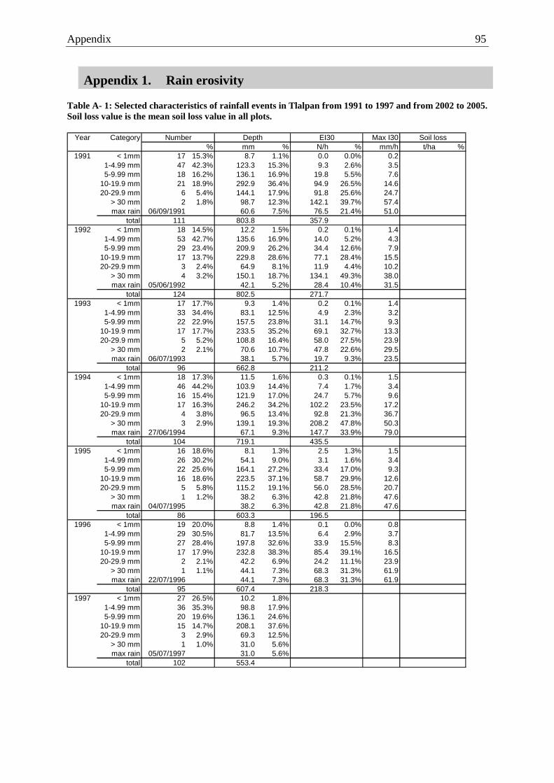
Appendix 95
Appendix 1. Rain erosivity
Table A- 1: Selected characteristics of rainfall events in Tlalpan from 1991 to 1997 and from 2002 to 2005.Soil loss value is the mean soil loss value in all plots.
Year Category Max I30% mm % N/h % mm/h t/ha %
1991 < 1mm 17 15.3% 8.7 1.1% 0.0 0.0% 0.21-4.99 mm 47 42.3% 123.3 15.3% 9.3 2.6% 3.55-9.99 mm 18 16.2% 136.1 16.9% 19.8 5.5% 7.6
10-19.9 mm 21 18.9% 292.9 36.4% 94.9 26.5% 14.620-29.9 mm 6 5.4% 144.1 17.9% 91.8 25.6% 24.7
> 30 mm 2 1.8% 98.7 12.3% 142.1 39.7% 57.4max rain 06/09/1991 60.6 7.5% 76.5 21.4% 51.0
total 111 803.8 357.91992 < 1mm 18 14.5% 12.2 1.5% 0.2 0.1% 1.4
1-4.99 mm 53 42.7% 135.6 16.9% 14.0 5.2% 4.35-9.99 mm 29 23.4% 209.9 26.2% 34.4 12.6% 7.9
10-19.9 mm 17 13.7% 229.8 28.6% 77.1 28.4% 15.520-29.9 mm 3 2.4% 64.9 8.1% 11.9 4.4% 10.2
> 30 mm 4 3.2% 150.1 18.7% 134.1 49.3% 38.0max rain 05/06/1992 42.1 5.2% 28.4 10.4% 31.5
total 124 802.5 271.71993 < 1mm 17 17.7% 9.3 1.4% 0.2 0.1% 1.4
1-4.99 mm 33 34.4% 83.1 12.5% 4.9 2.3% 3.25-9.99 mm 22 22.9% 157.5 23.8% 31.1 14.7% 9.3
10-19.9 mm 17 17.7% 233.5 35.2% 69.1 32.7% 13.320-29.9 mm 5 5.2% 108.8 16.4% 58.0 27.5% 23.9
> 30 mm 2 2.1% 70.6 10.7% 47.8 22.6% 29.5max rain 06/07/1993 38.1 5.7% 19.7 9.3% 23.5
total 96 662.8 211.21994 < 1mm 18 17.3% 11.5 1.6% 0.3 0.1% 1.5
1-4.99 mm 46 44.2% 103.9 14.4% 7.4 1.7% 3.45-9.99 mm 16 15.4% 121.9 17.0% 24.7 5.7% 9.6
10-19.9 mm 17 16.3% 246.2 34.2% 102.2 23.5% 17.220-29.9 mm 4 3.8% 96.5 13.4% 92.8 21.3% 36.7
> 30 mm 3 2.9% 139.1 19.3% 208.2 47.8% 50.3max rain 27/06/1994 67.1 9.3% 147.7 33.9% 79.0
total 104 719.1 435.51995 < 1mm 16 18.6% 8.1 1.3% 2.5 1.3% 1.5
1-4.99 mm 26 30.2% 54.1 9.0% 3.1 1.6% 3.45-9.99 mm 22 25.6% 164.1 27.2% 33.4 17.0% 9.3
10-19.9 mm 16 18.6% 223.5 37.1% 58.7 29.9% 12.620-29.9 mm 5 5.8% 115.2 19.1% 56.0 28.5% 20.7
> 30 mm 1 1.2% 38.2 6.3% 42.8 21.8% 47.6max rain 04/07/1995 38.2 6.3% 42.8 21.8% 47.6
total 86 603.3 196.51996 < 1mm 19 20.0% 8.8 1.4% 0.1 0.0% 0.8
1-4.99 mm 29 30.5% 81.7 13.5% 6.4 2.9% 3.75-9.99 mm 27 28.4% 197.8 32.6% 33.9 15.5% 8.3
10-19.9 mm 17 17.9% 232.8 38.3% 85.4 39.1% 16.520-29.9 mm 2 2.1% 42.2 6.9% 24.2 11.1% 23.9
> 30 mm 1 1.1% 44.1 7.3% 68.3 31.3% 61.9max rain 22/07/1996 44.1 7.3% 68.3 31.3% 61.9
total 95 607.4 218.31997 < 1mm 27 26.5% 10.2 1.8%
1-4.99 mm 36 35.3% 98.8 17.9%5-9.99 mm 20 19.6% 136.1 24.6%
10-19.9 mm 15 14.7% 208.1 37.6%20-29.9 mm 3 2.9% 69.3 12.5%
> 30 mm 1 1.0% 31.0 5.6%max rain 05/07/1997 31.0 5.6%
total 102 553.4
Number Depth EI30 Soil loss

Appendix 96
Table A-1 (follow) Selected characteristics of rainfall events in Tlalpan from 1991 to 1997 and from 2002to 2005. Soil loss value is the mean soil loss value in all plots
Year Category Max I30% mm % N/h % mm/h t/ha %
2002 < 1mm 66 44.6% 25.5 4.8% 0.2 0.1% 0.61-4.99 mm 55 37.2% 131.4 24.8% 9.4 5.1% 3.35-9.99 mm 10 6.8% 74.1 14.0% 15.3 8.3% 9.4
10-19.9 mm 12 8.1% 164.5 31.0% 68.5 37.2% 17.720-29.9 mm 4 2.7% 101.9 19.2% 41.4 22.5% 20.2
> 30 mm 1 0.7% 32.7 6.2% 49.2 26.8% 57.6max rain 30/10/2002 32.7 6.2% 49.2 26.8% 57.6
total 148 530.1 184.0
2003 < 1mm 123 56.2% 39.5 4.9% 0.1 0.0% 0.21-4.99 mm 50 22.8% 119.9 14.9% 7.7 2.2% 3.1 0.03 0.3%5-9.99 mm 17 7.8% 108.9 13.5% 15.8 4.6% 7.3 0.46 4.8%
10-19.9 mm 21 9.6% 297.3 36.9% 121.8 35.3% 18.1 3.70 38.7%20-29.9 mm 5 2.3% 125.1 15.5% 83.3 24.1% 29.9 0.62 6.5%
> 30 mm 3 1.4% 114.7 14.2% 116.2 33.7% 41.0 4.74 49.6%max rain 02/06/2003 40.8 5.1% 22.7 6.6% 13.9 0.30 3.1%
total 219 805.4 344.9 9.542004 < 1mm 161 60.5% 46.7 6.2% 0.3 0.1% 0.3
1-4.99 mm 64 24.1% 152.9 20.2% 11.9 3.2% 3.5 0.04 0.6%
5-9.99 mm 18 6.8% 128.9 17.1% 25.1 6.7% 9.4 0.20 2.6%10-19.9 mm 18 6.8% 259.8 34.4% 117.6 31.2% 18.4 1.90 24.7%20-29.9 mm 4 1.5% 103.7 13.7% 83.8 22.3% 33.4 2.68 34.8%
> 30 mm 1 0.4% 63.8 8.4% 138.0 36.6% 79.2 2.88 37.4%max rain 17/09/2004 63.8 8.4% 138.0 36.6% 27.9 2.24 29.1%
total 266 755.8 376.7 7.712005 < 1mm 152 66.4% 44.5 7.7% 0.2 0.1% 0.2
1-4.99 mm 43 18.8% 103.2 17.9% 8.3 4.3% 3.4 0.00 0.0%5-9.99 mm 17 7.4% 126.8 22.0% 22.9 11.7% 8.9 0.23 6.3%
10-19.9 mm 14 6.1% 209.4 36.3% 81.5 41.7% 16.7 1.92 53.5%
20-29.9 mm 2 0.9% 50.0 8.7% 46.1 23.6% 37.3 0.02 0.5%> 30 mm 1 0.4% 43.6 7.6% 36.3 18.6% 37.3 1.42 39.7%max rain 31/08/2005 43.6 7.6% 36.3 18.6% 12.4 0.36 10.0%
total 229 577.4 195.3 3.6Mean < 1mm 57.6 40.1% 20.5 3.0% 0.4 0.1% 0.8
(1991-2005) 1-4.99 mm 43.8 30.5% 108.0 16.0% 8.3 3.0% 3.5 0.02 0.3%5-9.99 mm 19.6 13.7% 142.0 21.0% 25.6 9.2% 8.7 0.30 4.3%
10-19.9 mm 16.8 11.7% 236.2 35.0% 87.7 31.4% 16.1 2.50 36.1%20-29.9 mm 3.9 2.7% 92.9 13.8% 58.9 21.1% 26.1 1.11 15.9%
> 30 mm 1.8 1.3% 75.1 11.1% 98.3 35.2% 50.0 3.01 43.4%
max rain 45.6 6.8% 63.0 22.5% 40.6 0.97 13.9%total 143.6 674.6 279.2 6.9
Depth EI30 Soil lossNumber

Appendix 97
Appendix 2. Soil loss and runoff
Table A- 2: Annual soil loss, runoff, runoff coefficient and sediment discharge in Tlalpan. Different letterindicates significant difference at P<0.05.
86-I 86-O 86-C 02-C 02-O
Soil loss 2003 4.5 5.5 4.6 19.1 14.1
2004 2.3 4.2 5.6 16.2 10.2
2005 1.1 1.4 1.3 8.6 5.5
Mean 2.6 3.7 3.8 14.6 9.9
P<0.05 a a a b c
Runoff 2003 51.2 49.3 70.4 265.2 169.2
2004 57.0 81.7 98.2 209.0 146.1
2005 26.2 31.4 39.2 164.9 140.4
Mean 44.8 54.1 69.3 213.0 151.9
p<0.05 a a a b c
Runoff coefficient 2003 10% 10% 13% 42% 26%
2004 13% 20% 24% 46% 30%
2005 11% 11% 14% 48% 36%
Mean 11% 14% 17% 45% 31%
sediment discharge 2003 43.3 50.4 47.7 78.3 63.3
2004 36.8 53.0 56.4 68.3 60.8
2005 35.5 37.8 42.7 48.8 38.8
Mean 38.5 47.1 48.9 65.1 54.3

Appendix 98
Table A- 3: Distribution of soil loss by rainfall event size from 2003 to 2005 in Tlalpan.
Soil lossyear category number ton/ha % ton/ha % ton/ha % ton/ha % ton/ha % ton/ha %
2003 1-4.99 mm 2 0.12 1% 0.01 0% 0.13 0%5-9.99 mm 6 0.18 4% 0.18 3% 0.17 4% 1.02 5% 0.76 5% 2.31 5%10-19.9 mm 17 0.96 22% 1.55 28% 1.62 36% 8.54 45% 5.80 41% 18.48 39%20-29.9 mm 5 0.05 1% 0.05 1% 0.15 3% 2.22 12% 0.65 5% 3.11 7%> 30 mm 4 3.28 73% 3.71 68% 2.61 57% 7.17 38% 6.90 49% 23.68 50%Max (42.1 mm) 30/06/03 3.23 72% 3.68 67% 2.40 53% 3.53 19% 5.32 38% 18.16 38%
Total 34 4.46 5.48 4.55 19.07 14.13 47.702004 1-4.99 mm 3 0.14 1% 0.06 1% 0.20 1%
5-9.99 mm 3 0.03 2% 0.13 3% 0.11 2% 0.40 2% 0.33 3% 1.01 3%10-19.9 mm 9 0.29 13% 0.92 22% 1.15 21% 5.20 32% 1.96 19% 9.52 25%20-29.9 mm 5 0.80 35% 1.68 40% 2.13 38% 5.70 35% 3.07 30% 13.39 35%> 30 mm 2 1.16 51% 1.49 35% 2.20 39% 4.74 29% 4.81 47% 14.40 37%Max (63.8 mm) 17/09/04 0.90 39% 1.09 26% 1.61 29% 3.48 22% 4.14 40% 11.21 29%Total 22 2.28 4.24 5.59 16.18 10.23 38.53
2005 1-4.99 mm5-9.99 mm 4 0.02 2% 0.07 5% 0.06 5% 0.61 7% 0.36 7% 1.13 6%
10-19.9 mm 11 0.70 65% 0.81 58% 0.98 74% 4.18 48% 2.91 53% 9.58 54%20-29.9 mm 1 0.07 1% 0.02 0% 0.09 0%> 30 mm 3 0.36 33% 0.51 37% 0.28 21% 3.76 44% 2.19 40% 7.10 40%Max (17.5 mm) 28/07/05 0.49 45% 0.42 30% 0.63 48% 1.99 23% 1.47 27% 5.00 28%Total 19 1.08 1.40 1.31 8.62 5.48 17.89
Mean 1-4.99 mm 2.5 0.13 1% 0.04 0% 0.16 0%5-9.99 mm 4.3 0.08 3% 0.13 3% 0.12 3% 0.68 5% 0.48 5% 1.48 4%10-19.9 mm 12.3 0.65 25% 1.09 29% 1.25 33% 5.97 41% 3.56 36% 12.52 36%20-29.9 mm 3.7 0.42 16% 0.87 23% 1.14 30% 2.66 18% 1.25 13% 6.34 18%> 30 mm 3.0 1.60 61% 1.90 51% 1.70 44% 5.23 36% 4.63 47% 15.06 43%
Max 1.54 59% 1.73 47% 1.55 40% 3.00 21% 3.65 37% 11.46 33%Total 25.0 2.61 3.71 3.82 14.63 9.95 34.71
02-O (R2) Total86-I (C) 86-O (D) 86-C (E) 02-C (R1)
Table A- 4: Distribution of runoff by rainfall event category from 2003 to 2005 in Tlalpan.
RunoffYear category number mm % mm % mm % mm % mm % mm %2003 1-4.99 mm 2 3.5 1% 0.4 0% 3.9 1%
5-9.99 mm 6 1.8 4% 1.8 4% 2.6 4% 12.5 5% 5.2 3% 24.0 4%10-19.9 mm 17 20.4 40% 19.2 39% 21.5 30% 98.6 37% 70.2 41% 229.9 38%20-29.9 mm 5 5.1 10% 5.0 10% 12.0 17% 69.7 26% 25.3 15% 117.0 19%> 30 mm 4 23.9 47% 23.4 47% 34.3 49% 80.8 30% 68.1 40% 230.5 38%Max (42.1 mm) 30/06/03 20.9 41% 21.0 43% 25.3 36% 37.2 14% 37.0 22% 141.4 23%Total 34 51.2 49.3 70.4 265.2 169.2 605.3
2004 1-4.99 mm 3 0.3 0% 2.8 1% 1.2 1% 4.2 1%5-9.99 mm 3 1.1 2% 2.6 3% 1.3 1% 5.2 2% 4.4 3% 14.6 2%10-19.9 mm 9 8.8 15% 17.9 22% 22.0 22% 70.7 34% 34.3 23% 153.7 26%20-29.9 mm 5 18.0 32% 31.1 38% 36.5 37% 68.7 33% 50.2 34% 204.5 35%> 30 mm 2 29.1 51% 29.8 36% 38.4 39% 61.6 29% 56.0 38% 215.0 36%Max (63.8 mm) 17/09/04 25.4 44% 25.2 31% 32.1 33% 43.4 21% 45.8 31% 171.8 29%Total 22 57.0 81.7 98.2 209.0 146.1 592.0
2005 1-4.99 mm 0.0 0%5-9.99 mm 4 0.6 2% 3.0 9% 1.6 4% 10.3 6% 8.8 6% 24.2 6%10-19.9 mm 11 13.3 51% 17.0 54% 14.4 37% 66.2 40% 48.3 34% 159.3 40%20-29.9 mm 1 6.3 4% 2.7 2% 9.0 2%> 30 mm 3 12.4 47% 11.4 36% 23.2 59% 82.1 50% 80.5 57% 209.6 52%Max (43.6 mm) 31/08/05 5.5 21% 7.0 22% 9.5 24% 24.2 15% 37.1 26% 83.3 21%Total 19 26.2 31.4 39.2 164.9 140.4 402.1
Mean 1-4.99 mm 2.5 0.3 1% 3.1 1% 0.8 1% 4.2 1%5-9.99 mm 4.3 1.1 3% 2.5 5% 1.8 3% 9.3 4% 6.1 4% 20.9 4%10-19.9 mm 12.3 14.2 32% 18.0 33% 19.3 28% 78.5 37% 50.9 34% 180.9 34%20-29.9 mm 3.7 11.5 26% 18.0 33% 24.2 35% 48.2 23% 26.1 17% 128.1 24%> 30 mm 3.0 21.8 49% 21.5 40% 32.0 46% 74.9 35% 68.2 45% 218.4 41%
17.3 39% 17.7 33% 22.3 32% 34.9 16% 39.9 26% 132.2 25%Total 25.0 44.8 54.1 69.3 213.0 151.9 533.1
02-O (R2) Total86-I (C) 86-O (D) 86-C (E) 02-C (R1)

Appendix 99
Appendix 3. Vegetation cover
Table A- 5: Vegetation cover measured in Tlalpan from 2002 to 2005. Different letter indicates significantdifference (ANOVA repeated measures)
Year Date Days* 86-C 86-I 86-O 02-C 02-O2002 12-Jul 27 13.5% 20.9% 14.1%
05-Aug 50 22.0% 28.4% 24.4% 8.3% 20.4%12-Aug 57 24.2% 20.9% 27.7% 12.6% 28.7%29-Aug 74 29.8% 38.5% 35.7% 29.5% 20.9%10-Sep 85 44.6% 41.5% 30.4% 34.9% 19.4%18-Sep 93 47.5% 42.1% 64.0% 20.5% 27.8%25-Sep 100 44.2% 46.3% 58.6% 40.6% 37.9%01-Oct 106 78.8% 75.8% 64.5% 32.1% 39.0%21-Oct 126 76.1% 76.3% 71.0% 41.2% 36.0%12-Nov 147 55.0% 67.0% 69.7% 31.1% 43.6%Mean 43.5% 46.1% 46.0% 27.9% 30.4%P<0.05 a a a b b
2003 14-Jul 31 41.3% 60.8% 48.6% 33.2% 46.9%24-Jul 41 69.8% 91.0% 72.4% 45.9% 79.1%
07-Aug 54 82.0% 98.1% 95.8% 44.5% 85.0%26-Aug 73 68.5% 90.9% 94.1% 38.8% 89.6%22-Sep 99 37.6% 87.4% 64.0% 33.5% 85.0%Mean 60.9% 83.9% 73.6% 39.2% 77.1%P<0.05 a b c d c
2004 Estimation 100 77.5% 87.5% 79.0% 35.0% 70.0%+- 5% +- 5% +- 5% +- 5% +- 5%
2005 20-Jul 28 2.1% 8.9% 6.3% 5.2% 4.6%28-Jul 36 8.3% 21.1% 18.8% 10.1% 11.3%
05-Aug 43 18.3% 48.4% 38.9% 16.6% 18.2%11-Aug 49 40.3% 67.4% 56.8% 31.5% 30.6%18-Aug 56 66.3% 80.7% 74.5% 35.1% 37.1%25-Aug 63 78.1% 86.6% 81.1% 42.2% 43.5%01-Sep 69 76.4% 82.7% 86.4% 43.0% 61.4%08-Sep 76 71.2% 86.4% 86.2% 34.7% 43.0%15-Sep 83 72.3% 89.1% 86.8% 45.0% 57.4%22-Sep 90 76.2% 88.5% 88.1% 46.0% 55.5%29-Sep 97 77.7% 89.5% 89.4% 50.5% 56.7%06-Oct 104 80.9% 89.6% 91.5% 54.5% 63.2%13-Oct 111 75.5% 90.8% 90.0% 39.2% 44.5%20-Oct 118 67.2% 90.3% 83.8% 34.7% 43.6%27-Oct 125 62.2% 83.4% 79.9% 27.5% 32.5%03-Nov 131 47.9% 70.4% 64.0% 32.2% 29.0%Mean 54.2% 69.0% 65.9% 32.2% 37.2%P<0.05 a b b c c
* Number of days after sowing.
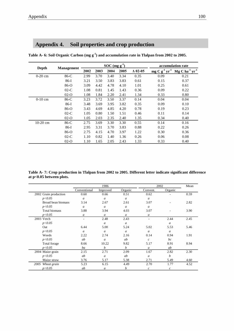
Appendix 100
Appendix 4. Soil properties and crop production
Table A- 6: Soil Organic Carbon (mg g-1) and accumulation rate in Tlalpan from 2002 to 2005.
2002 2003 2004 2005 Δ 02-05 mg C g-1 yr-1 Mg C ha-1 yr-1
0-20 cm 86-C 2.99 3.70 3.40 3.34 0.35 0.09 0.2186-I 3.21 3.50 3.83 3.83 0.61 0.15 0.3786-O 3.09 4.42 4.78 4.10 1.01 0.25 0.6102-C 1.08 0.81 1.45 1.43 0.36 0.09 0.2202-O 1.08 1.84 2.20 2.41 1.34 0.33 0.80
0-10 cm 86-C 3.23 3.72 3.50 3.37 0.14 0.04 0.0486-I 3.48 3.69 3.95 3.82 0.35 0.09 0.1086-O 3.43 4.69 4.85 4.20 0.78 0.19 0.2302-C 1.05 0.80 1.50 1.51 0.46 0.11 0.1402-O 1.05 2.03 2.35 2.40 1.35 0.34 0.40
10-20 cm 86-C 2.75 3.69 3.30 3.30 0.55 0.14 0.1686-I 2.95 3.31 3.70 3.83 0.88 0.22 0.2686-O 2.75 4.15 4.70 3.97 1.22 0.30 0.3602-C 1.10 0.82 1.40 1.36 0.26 0.06 0.0802-O 1.10 1.65 2.05 2.43 1.33 0.33 0.40
Depth ManagementSOC (mg g
-1) accumulation rate
Table A- 7: Crop production in Tlalpan from 2002 to 2005. Different letter indicate significant differenceat p<0.05 between plots.
MeanConventional Improved Organic Convent. Organic
2002 Grain production 0.60 0.66 0.51 0.62 - 0.59p<0.05 a a a aBroad bean biomass 3.14 2.67 2.61 3.07 - 2.82p<0.05 a a a aTotal biomass 3.88 3.94 4.03 3.07 - 3.90p<0.05 a a a a
2003 Vetch - 2.48 2.43 - 2.44 2.45p<0.05 a a aOat 6.44 5.00 5.24 5.02 5.53 5.46p<0.05 a a a a aWeeds 2.22 2.74 2.16 0.14 0.94 1.91p<0.05 ab a ab c bc
Total forage 8.66 10.22 9.82 5.17 8.91 8.94p<0.05 ba b b a ab
2004 Maize grain 2.15 2.71 2.09 1.67 2.82 2.30p<0.05 ab a ab a bMaize straw 3.76 5.17 5.38 2.71 5.49 4.60
2005 Wheat grain 5.23 6.15 4.49 2.70 1.77 4.52p<0.05 ab a b c c
1986 2002
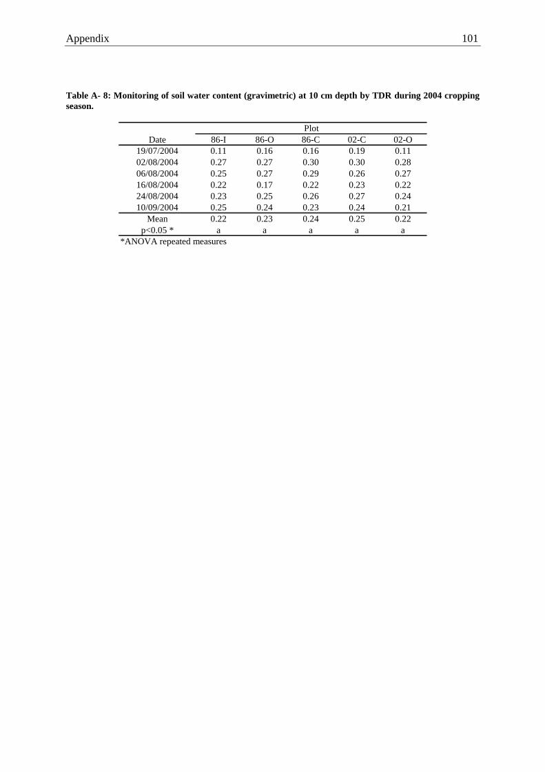
Appendix 101
Table A- 8: Monitoring of soil water content (gravimetric) at 10 cm depth by TDR during 2004 croppingseason.
Date 86-I 86-O 86-C 02-C 02-O19/07/2004 0.11 0.16 0.16 0.19 0.1102/08/2004 0.27 0.27 0.30 0.30 0.2806/08/2004 0.25 0.27 0.29 0.26 0.2716/08/2004 0.22 0.17 0.22 0.23 0.2224/08/2004 0.23 0.25 0.26 0.27 0.2410/09/2004 0.25 0.24 0.23 0.24 0.21
Mean 0.22 0.23 0.24 0.25 0.22p<0.05 * a a a a a
*ANOVA repeated measures
Plot

Appendix 102
Table A- 9: Monitoring of soil water content (gravimetric) by tensiometers in 2005 (weighted averagefrom measures done at 5, 10, 15, 25 and 40 cm depth).
86-I 86-O 86-C 02-C 02-O07/07/05 0.27 0.24 0.22 0.20 0.1815/07/05 0.20 0.23 0.20 0.20 0.1420/07/05 0.22 0.23 0.19 0.20 0.1525/07/05 0.22 0.23 0.20 0.21 0.1627/07/05 0.28 0.30 0.30 0.32 0.2628/07/05 0.28 0.31 0.31 0.31 0.2705/08/05 0.18 0.23 0.32 0.19 0.2008/08/05 0.29 0.27 0.31 0.24 0.2611/08/05 0.28 0.26 0.30 0.23 0.2514/08/05 0.34 0.25 0.45 0.23 0.2515/08/05 0.34 0.23 0.37 0.22 0.2418/08/05 0.32 0.21 0.40 0.22 0.1821/08/05 0.35 0.20 0.42 0.16 0.2122/08/05 0.33 0.22 0.38 0.16 0.2123/08/05 0.36 0.26 0.42 0.20 0.25
25/08/05 0.40 0.35 0.41 0.29 0.3001/09/05 0.42 0.31 0.42 0.18 0.2608/09/05 0.36 0.26 0.33 0.14 0.1609/09/05 0.40 0.38 0.41 0.25 0.2813/09/05 0.38 0.34 0.40 0.20 0.2215/09/05 0.36 0.28 0.35 0.15 0.2219/09/05 0.40 0.29 0.42 0.19 0.2122/09/05 0.36 0.27 0.34 0.24 0.2129/09/05 0.27 0.15 0.24 0.18 0.1704/10/05 0.24 0.14 0.17 0.17 0.1905/10/05 0.32 0.23 0.31 0.21 0.2206/10/05 0.40 0.31 0.39 0.22 0.2708/10/05 0.45 0.45 0.45 0.27 0.3712/10/05 0.45 0.45 0.45 0.36 0.4013/10/05 0.44 0.45 0.43 0.40 0.3920/10/05 0.39 0.43 0.35 0.37 0.3127/10/05 0.32 0.36 0.26 0.23 0.25
Mean 0.33 0.28 0.34 0.23 0.24p<0.05 * a ab a b b
*ANOVA repeated measures

Appendix 103
Appendix 5. Soil loss and runoff prediction
Table A- 10 Data set used in the multiple regression
86-I 86-O 86-C 02-C 02-O TOTAL2003 9 8 8 12 11 482004 11 12 12 13 13 612005 5 5 5 9 8 32
TOTAL 25 25 25 34 32 1412003 36% 33% 33% 34% 32% 34%2004 73% 71% 75% 59% 62% 67%2005 45% 29% 42% 50% 42% 42%
TOTAL 49% 43% 48% 45% 43% 45%2003 89% 90% 92% 64% 70% 74%2004 90% 81% 84% 84% 82% 83%2005 95% 77% 84% 69% 73% 74%
TOTAL 90% 85% 87% 72% 75% 77%
Number of events in the model
% of events kept in the model
% of annual soil loss considered
in the model
Table A- 11: Descriptive statistics of the variable used in the multiple regression
RUNOFF SOIL LOSS DEPTH KE wisch I10 max I30 max EI10 EI30 SOC COVERN 141 141 141 141 141 141 141 141 141 141Minimum 0.37 6.51 6.60 1.24 8.65 6.96 12.70 10.22 0.80 0.00Maximum 45.75 5324.37 63.80 17.42 109.47 79.20 1379.53 1379.53 4.54 0.95Median 4.81 260.66 17.09 4.07 42.95 27.45 179.52 105.91 3.32 0.43Skewness 2.06 3.01 1.67 1.98 0.79 1.36 2.00 3.27 -0.21 0.09Std. Error of Skewness 0.20 0.20 0.20 0.20 0.20 0.20 0.20 0.20 0.20 0.20Kurtosis 4.42 10.21 3.19 4.95 0.13 2.02 3.74 11.47 -1.29 -1.26Std. Error of Kurtosis 0.41 0.41 0.41 0.41 0.41 0.41 0.41 0.41 0.41 0.41
Table A- 12: Pearson coefficient of linear regression between soil loss and runoff and selected rainerosivity parameters
Variable Predictor 86-I 86-O 86-C 02-C 02-O ALL averagen=25 n=25 n=25 n=34 n=32 n=141
LOGerosion LOGdepth 0.45 0.33 0.38 0.66 0.55 0.41 0.48LOGKe 0.45 0.36 0.40 0.73 0.62 0.44 0.51LOGI10 0.43 0.39 0.33 0.79 0.70 0.45 0.53LOGI30 0.38 0.40 0.34 0.72 0.61 0.41 0.49LOGEI30 0.43 0.39 0.38 0.75 0.63 0.44 0.52LOGEI10 0.47 0.39 0.39 0.79 0.69 0.47 0.55
LOGrunoff LOGdepth 0.70 0.70 0.72 0.86 0.83 0.65 0.77LOGKe 0.70 0.70 0.72 0.90 0.86 0.66 0.78LOGI10 0.59 0.51 0.49 0.77 0.79 0.52 0.63LOGI30 0.61 0.66 0.63 0.85 0.77 0.58 0.71LOGEI30 0.68 0.71 0.70 0.90 0.85 0.64 0.77LOGEI10 0.69 0.65 0.65 0.88 0.87 0.62 0.75

Appendix 104
Table A- 13: Model summary and coefficients of multiple regression analysis for single event soil loss andrunoff prediction in reclaimed tepetates
Variable Predictor Standardized Coeff. R2
R2
Change
B S.E. Beta
LOGerosion (Constant) 1.741 0.172
COVER -1.017 0.113 -0.490 0.260 0.260
LOGEI10 0.677 0.069 0.525 0.521 0.262
SOC -0.160 0.028 -0.314 0.616 0.094
LOGerosion (Constant) 1.958 0.153
COVER -1.087 0.113 -0.524 0.260 0.260
LOGEI30 0.657 0.0662 0.530 0.529 0.270
SOC -0.154 0.027 -0.303 0.617 0.088
LOGerosion (Constant) 1.651 0.193
COVER -1.111 0.118 -0.535 0.260 0.260
LOGdepth 1.287 0.141 0.505 0.514 0.255
SOC -0.144 0.028 -0.282 0.591 0.076
LOGrunoff (Constant) -0.325 0.124
LOGdepth 1.284 0.091 0.695 0.427 0.427
SOC -0.150 0.018 -0.408 0.633 0.206
COVER -0.335 0.076 -0.223 0.679 0.046
LOGrunoff (Constant) 0.046 0.102
LOGEI30 0.621 0.0442 0.691 0.411 0.411
SOC -0.161 0.018 -0.436 0.638 0.227
COVER -0.303 0.076 -0.201 0.676 0.038
LOGrunoff (Constant) -0.113 0.120
LOGEI10 0.618 0.048 0.662 0.389 0.389
SOC -0.166 0.019 -0.450 0.620 0.231
COVER -0.234 0.079 -0.156 0.643 0.023
LOGerosion (Constant) 1.959 0.057
LOGrunoff 1.046 0.052 0.759 0.686 0.686
COVER -0.756 0.078 -0.364 0.814 0.128
Unstandardized Coeff.
Table A- 14: Model summary and coefficients of multiple regression analysis for annual soil loss andrunoff prediction in reclaimed tepetates.
Variable Predictor Standardized Coeff. R 2 R2 ChangeB S.E. Beta (adjusted)
Soil loss (Constant) 9.75 2.73SOC -3.98 0.51 -0.83 0.64 0.64EI30 0.030 0.01 0.44 0.84 0.20
Soil loss (Constant) -4.83 1.95Runoff 0.07 0.01 0.88 0.85 0.85EI30 0.015 0.01 0.21 0.89 0.04
Runoff (Constant) 265.23 34.15SOC -37.50 8.16 -0.61 0.79 0.79Vmax -144.82 50.72 -0.38 0.85 0.06EI30 0.207 0.07 0.23 0.91 0.05
Unstandardized Coeff.

Appendix 105
Appendix 6. Aggregation
Table A- 15: Dry aggregate size distribution and Mean Weight Diameter (MWD) in Tlalpan. Differentletter indicate significant difference (P<0.05) in mean MWD between plots (a, b, c) and between age ofrehabilitation (x, y).
Year of Management Year MWDrehab. 10 - 8 8 - 5 5 - 3.15 3.15 - 2 2 - 1 < 1 1 - 0.59 < 0.591986 Conventional 2003 12.0% 16.3% 14.6% 12.5% 9.9% 34.6% 3.38
2004 7.1% 11.5% 11.1% 8.8% 13.2% *48.3% 12.4% 36.0% 2.472005 11.1% 14.3% 14.7% 11.5% 12.2% *36.2% 12.5% 23.6% 3.18
Mean 10.9% 15.0% 13.9% 11.6% 11.0% 34.6% 12.4% 30.7% 3.14 abImproved 2003 11.8% 14.7% 14.1% 11.9% 9.7% 37.8% 3.23
2004 6.1% 10.9% 12.2% 9.4% 13.8% *47.5% 12.0% 35.5% 2.412005 8.8% 12.7% 15.4% 12.0% 12.2% *38.9% 12.2% 26.8% 2.91
Mean 10.1% 13.6% 13.9% 11.4% 11.0% 37.8% 12.1% 31.8% 2.99 aOrganic 2003 12.7% 17.6% 16.0% 12.2% 9.5% 32.0% 3.55
2004 8.4% 12.4% 12.8% 9.8% 12.7% *43.9% 11.7% 32.2% 2.722005 7.6% 12.3% 14.7% 12.2% 13.5% *39.7% 15.3% 24.4% 2.79
Mean 11.0% 15.7% 15.1% 11.7% 10.8% 32.0% 13.2% 28.9% 3.23 bMean 10.7% 14.7% 14.3% 11.6% 10.9% 34.8% 12.6% 30.4% 3.12 x
2002 Conventional 2003 11.5% 13.1% 12.1% 11.2% 9.7% 42.4% 3.032004 6.9% 9.5% 12.3% 9.4% 11.3% *50.5% 16.7% 33.8% 2.392005 5.4% 9.7% 12.0% 10.5% 13.4% *48.9% 17.2% 31.7% 2.31
Mean 9.0% 11.5% 12.1% 10.7% 11.0% 42.4% 17.0% 32.5% 2.69 cOrganic 2003 9.2% 12.7% 13.0% 13.9% 9.1% 42.2% 2.88
2004 8.6% 11.5% 11.7% 9.8% 14.2% *44.1% 12.6% 31.6% 2.662005 6.0% 9.5% 9.5% 10.8% 14.1% *50.1% 18.5% 31.6% 2.28
Mean 8.2% 11.6% 11.8% 12.3% 11.4% 42.2% 16.1% 31.6% 2.66 cMean 8.6% 11.6% 12.0% 11.5% 11.2% 42.3% 16.6% 32.1% 2.67 y
Mean 10.1% 13.9% 13.7% 11.5% 11.0% 36.7% 13.9% 31.0% 2.99* In 2004 and 2005, the fraction <1 mm is the sum of 1-0.59 and <0.59 mm fractionsMWD: Mean weight diameterSD: Standard deviation
Aggregate size (mm)
Table A- 16: Evolution of ASD and MWD during the 2005 cropping season in Tlalpan. Different letterindicates significant difference (P<0.05) in MWD between 2002-plots and 1986-plots within a date.
Date Year Management < 0.59 mm 0.59 - 1 mm 1 - 2 mm 2 - 3.15 mm 3.15 - 5 mm 5 - 8 mm 8 - 10 mm MWD13/07/2005 1986 Conventional 30.5% 18.5% 9.5% 11.0% 11.1% 10.8% 8.7% 2.46
Improved 36.4% 17.1% 8.9% 10.8% 12.4% 9.0% 5.4% 1.99Organic 29.0% 23.8% 9.7% 11.3% 11.4% 9.0% 5.8% 2.08
Mean 32.0% 19.8% 9.3% 11.0% 11.6% 9.6% 6.6% 2.18 a2002 Conventional 36.7% 20.0% 9.4% 10.8% 11.2% 7.9% 4.0% 1.76
Organic 31.4% 23.9% 9.4% 11.0% 11.3% 8.0% 5.0% 1.95Mean 34.0% 22.0% 9.4% 10.9% 11.2% 8.0% 4.5% 1.85 a
22/09/2005 1986 Conventional 9.9% 7.5% 13.7% 13.0% 19.0% 20.2% 16.6% 3.98Improved 12.1% 6.7% 13.3% 14.6% 20.0% 18.6% 14.8% 3.76Organic 12.0% 9.8% 16.6% 14.9% 19.7% 17.5% 9.6% 3.03Mean 11.3% 8.0% 14.5% 14.2% 19.6% 18.8% 13.7% 3.59 a
2002 Conventional 27.5% 15.7% 15.8% 10.4% 13.2% 11.2% 6.2% 2.21Organic 30.8% 18.6% 17.0% 11.3% 6.2% 9.3% 6.7% 2.08Mean 29.2% 17.1% 16.4% 10.8% 9.7% 10.3% 6.5% 2.15 b
17/11/2005 1986 Conventional 30.5% 11.6% 13.5% 10.6% 14.1% 11.8% 8.1% 2.48Improved 31.8% 12.8% 14.3% 10.5% 13.8% 10.6% 6.2% 2.21Organic 32.3% 12.2% 14.1% 10.5% 13.1% 10.3% 7.5% 2.38Mean 31.5% 12.2% 14.0% 10.5% 13.6% 10.9% 7.3% 2.35 a
2002 Conventional 30.8% 16.0% 15.1% 10.4% 11.8% 10.0% 6.0% 2.12
Organic 32.7% 12.9% 15.8% 10.1% 10.9% 11.2% 6.4% 2.13Mean 31.8% 14.4% 15.5% 10.3% 11.3% 10.6% 6.2% 2.13 a
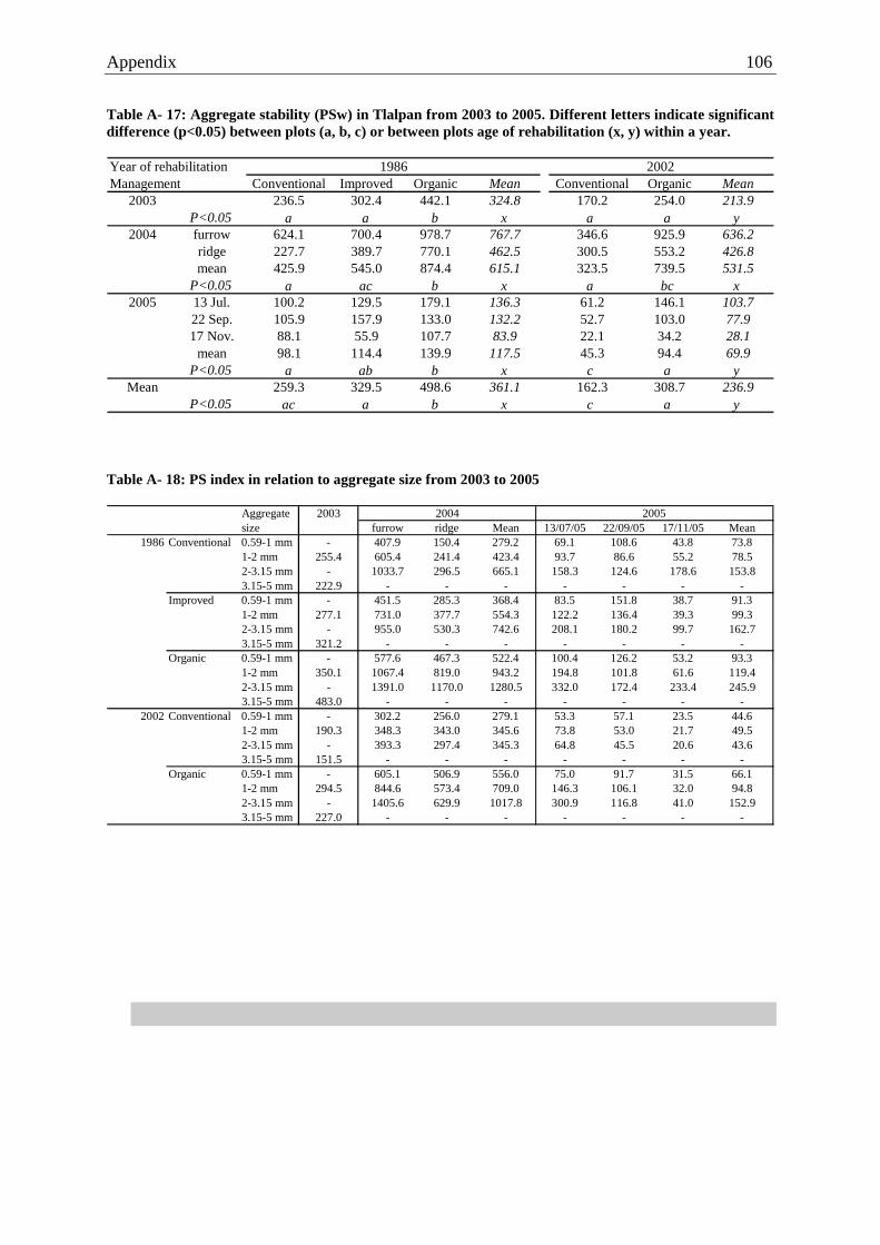
Appendix 106
Table A- 17: Aggregate stability (PSw) in Tlalpan from 2003 to 2005. Different letters indicate significantdifference (p<0.05) between plots (a, b, c) or between plots age of rehabilitation (x, y) within a year.
Year of rehabilitationManagement Conventional Improved Organic Mean Conventional Organic Mean
2003 236.5 302.4 442.1 324.8 170.2 254.0 213.9P<0.05 a a b x a a y
2004 furrow 624.1 700.4 978.7 767.7 346.6 925.9 636.2ridge 227.7 389.7 770.1 462.5 300.5 553.2 426.8mean 425.9 545.0 874.4 615.1 323.5 739.5 531.5
P<0.05 a ac b x a bc x2005 13 Jul. 100.2 129.5 179.1 136.3 61.2 146.1 103.7
22 Sep. 105.9 157.9 133.0 132.2 52.7 103.0 77.917 Nov. 88.1 55.9 107.7 83.9 22.1 34.2 28.1
mean 98.1 114.4 139.9 117.5 45.3 94.4 69.9P<0.05 a ab b x c a y
Mean 259.3 329.5 498.6 361.1 162.3 308.7 236.9P<0.05 ac a b x c a y
1986 2002
Table A- 18: PS index in relation to aggregate size from 2003 to 2005
Aggregate 2003size furrow ridge Mean 13/07/05 22/09/05 17/11/05 Mean
1986 Conventional 0.59-1 mm - 407.9 150.4 279.2 69.1 108.6 43.8 73.81-2 mm 255.4 605.4 241.4 423.4 93.7 86.6 55.2 78.52-3.15 mm - 1033.7 296.5 665.1 158.3 124.6 178.6 153.83.15-5 mm 222.9 - - - - - - -
Improved 0.59-1 mm - 451.5 285.3 368.4 83.5 151.8 38.7 91.31-2 mm 277.1 731.0 377.7 554.3 122.2 136.4 39.3 99.32-3.15 mm - 955.0 530.3 742.6 208.1 180.2 99.7 162.73.15-5 mm 321.2 - - - - - - -
Organic 0.59-1 mm - 577.6 467.3 522.4 100.4 126.2 53.2 93.31-2 mm 350.1 1067.4 819.0 943.2 194.8 101.8 61.6 119.42-3.15 mm - 1391.0 1170.0 1280.5 332.0 172.4 233.4 245.93.15-5 mm 483.0 - - - - - - -
2002 Conventional 0.59-1 mm - 302.2 256.0 279.1 53.3 57.1 23.5 44.61-2 mm 190.3 348.3 343.0 345.6 73.8 53.0 21.7 49.52-3.15 mm - 393.3 297.4 345.3 64.8 45.5 20.6 43.63.15-5 mm 151.5 - - - - - - -
Organic 0.59-1 mm - 605.1 506.9 556.0 75.0 91.7 31.5 66.11-2 mm 294.5 844.6 573.4 709.0 146.3 106.1 32.0 94.82-3.15 mm - 1405.6 629.9 1017.8 300.9 116.8 41.0 152.93.15-5 mm 227.0 - - - - - - -
2004 2005

Appendix 107
Appendix 7. Porosity
Table A- 19: Porosity and pore size distribution in 2003
Year = 2003 Meandepth Parameter Conv. Imp. Organic Mean Conv. Organic Mean
10 PT sat 42.7 42.8 45.1 43.5 48.2 43.9 45.9 44.1Bulk Density 1.2 1.3 1.2 1.2 1.1 1.2 1.2 1.2Fine pores <0.2 μm 18.9 19.6 17.4 18.7 18.2 20.2 19.3 18.8
Pores 0.2 - 3 μm 8.7 9.7 10.2 9.5 8.8 10.6 9.8 9.6Pores 3 - 10 μm 2.8 3.4 3.0 3.1 2.7 2.5 2.6 3.0Medium pores 0.2-10 μm 11.6 13.1 13.2 12.6 11.5 13.1 12.4 12.5Pores 10 - 30 μm 4.1 4.3 4.2 4.2 5.1 4.2 4.6 4.3Pores30 - 50 μm 2.0 1.8 2.1 1.9 3.1 2.1 2.6 2.1Pores 50 - 120 μm 3.3 2.4 4.4 3.4 5.5 3.5 4.4 3.6Pores >120μm 3.0 1.5 3.8 2.8 4.8 0.8 2.6 2.7Large pores >10 μm 12.3 10.0 14.5 12.3 18.5 10.6 14.2 12.8
20 PT sat 44.4 45.0 45.6 45.0 45.3 45.7 45.5 45.2Bulk Density 1.3 1.2 1.3 1.3 1.2 1.2 1.2 1.3Fine pores <0.2 μm 20.4 19.0 19.8 19.8 21.0 21.2 21.1 20.1Pores 0.2 - 3 μm 10.9 10.3 10.7 10.6 11.0 10.5 10.8 10.6Pores 3 - 10 μm 2.9 3.0 3.3 3.1 2.4 2.7 2.5 2.9Medium pores 0.2-10 μm 13.7 13.3 14.0 13.7 13.4 13.2 13.3 13.6Pores 10 - 30 μm 4.0 4.4 4.4 4.3 4.0 4.0 4.0 4.2Pores30 - 50 μm 1.9 2.0 1.9 2.0 2.5 2.1 2.3 2.0
Pores 50 - 120 μm 3.0 3.8 3.5 3.5 2.8 3.7 3.3 3.4Pores >120μm 1.3 2.5 2.0 1.9 1.6 1.6 1.6 1.8Large pores >10 μm 10.2 12.7 11.8 11.6 10.9 11.4 11.1 11.5
30 PT sat 43.7 45.2 45.8 45.0 44.6 44.9 44.7 44.9Bulk Density 1.3 1.3 1.2 1.2 1.3 1.2 1.2 1.2Fine pores <0.2 μm 20.4 20.8 19.4 20.2 21.7 22.5 22.1 20.7Pores 0.2 - 3 μm 8.6 8.7 10.2 9.2 10.6 9.5 10.0 9.4Pores 3 - 10 μm 3.3 3.1 2.9 3.1 2.3 2.1 2.2 2.8Medium pores 0.2-10 μm 11.8 11.8 13.1 12.3 12.8 11.6 12.2 12.3Pores 10 - 30 μm 4.2 4.2 4.6 4.3 3.6 3.0 3.3 4.1Pores30 - 50 μm 2.0 2.0 2.1 2.0 1.9 1.7 1.8 2.0Pores 50 - 120 μm 3.2 3.7 4.0 3.6 3.4 3.2 3.3 3.5Pores >120μm 2.2 2.7 2.7 2.5 1.2 2.8 2.0 2.4Large pores >10 μm 11.5 12.6 13.4 12.5 10.1 10.7 10.4 12.0
40 PT sat 43.6 45.8 45.5 45.0 46.6 43.9 45.1 45.0
Bulk Density 1.3 1.2 1.3 1.3 1.2 1.3 1.2 1.3Fine pores <0.2 μm 20.6 21.4 20.8 21.0 22.5 23.1 22.8 21.4Pores 0.2 - 3 μm 8.3 9.4 10.1 9.2 9.9 10.8 10.4 9.5Pores 3 - 10 μm 3.7 3.2 3.0 3.3 2.1 2.4 2.3 3.1Medium pores 0.2-10 μm 11.9 12.7 13.1 12.5 12.0 13.2 12.6 12.6Pores 10 - 30 μm 4.4 4.2 4.5 4.4 2.8 2.9 2.9 4.1Pores30 - 50 μm 2.1 1.8 2.3 2.1 1.5 1.7 1.6 2.0Pores 50 - 120 μm 2.9 3.2 3.1 3.1 3.2 2.1 2.6 3.0Pores >120μm 1.6 2.6 1.7 2.0 4.6 1.0 2.6 2.1Large pores >10 μm 11.0 11.8 11.6 11.5 12.1 7.7 9.7 11.1
Mean PT sat 43.6 44.8 45.5 44.6 46.1 44.6 45.3 44.8Bulk Density 1.3 1.3 1.2 1.3 1.2 1.2 1.2 1.2Fine pores <0.2 μm 20.1 20.3 19.4 19.9 20.8 21.7 21.3 20.2Pores 0.2 - 3 μm 9.1 9.5 10.3 9.7 10.2 10.3 10.2 9.8Pores 3 - 10 μm 3.2 3.2 3.1 3.1 2.4 2.4 2.4 2.9Medium pores 0.2-10 μm 12.3 12.7 13.4 12.8 12.5 12.8 12.7 12.7
Pores 10 - 30 μm 4.2 4.3 4.5 4.3 3.9 3.5 3.7 4.2Pores30 - 50 μm 2.0 1.9 2.1 2.0 2.3 1.9 2.1 2.0Pores 50 - 120 μm 3.1 3.3 3.7 3.4 3.7 3.2 3.4 3.4Pores >120μm 2.0 2.3 2.5 2.3 2.8 1.6 2.2 2.3Large pores >10 μm 11.3 11.8 12.8 12.0 12.7 10.2 11.4 11.8
1986 2002

Appendix 108
Table A- 20: Porosity and pore size distribution in 2004 (in ridge area)
Year = 2004 Meandepth Parameter Conv. Imp. Organic Mean Conv. Organic Mean
5 PT sat 47.8 47.1 45.3 46.7 46.0 50.3 48.2 47.1Bulk Density 1.2 1.2 1.2 1.2 1.2 1.1 1.2 1.2Fine pores <0.2 μm 15.5 14.6 15.0 15.0 16.9 18.8 17.8 15.7
Pores 0.2 - 3 μm 11.8 13.6 12.0 12.5 12.3 8.5 10.4 12.0Pores 3 - 10 μm 3.2 2.6 2.6 2.8 3.0 2.6 2.8 2.8Medium pores 0.2-10 μm 15.0 16.2 14.6 15.2 15.3 11.1 13.2 14.7Pores 10 - 30 μm 4.8 4.8 4.7 4.8 4.6 5.0 4.8 4.8Pores30 - 50 μm 2.2 2.6 2.2 2.4 2.1 2.8 2.5 2.4Pores 50 - 120 μm 4.5 3.9 4.1 4.2 3.6 4.8 4.2 4.2Pores >120μm 5.8 4.9 4.8 5.2 3.6 7.9 5.7 5.3Large pores >10 μm 17.4 16.2 15.8 16.4 13.9 20.4 17.2 16.6
10 PT sat 47.5 47.5 46.6 47.2 47.5 50.4 48.9 47.6Bulk Density 1.3 1.2 1.2 1.2 1.2 1.2 1.2 1.2Fine pores <0.2 μm 15.5 14.6 15.0 15.0 17.4 18.8 18.1 15.8Pores 0.2 - 3 μm 14.1 12.9 12.2 13.1 14.8 11.7 13.3 13.1Pores 3 - 10 μm 3.4 2.6 2.8 2.9 2.9 2.6 2.7 2.9Medium pores 0.2-10 μm 17.5 15.6 15.0 16.0 17.7 14.3 16.0 16.0Pores 10 - 30 μm 6.1 4.9 4.8 5.3 3.9 4.3 4.1 4.9
Pores30 - 50 μm 1.7 2.7 2.5 2.3 2.4 2.6 2.5 2.3Pores 50 - 120 μm 3.3 4.3 4.2 3.9 3.6 5.3 4.4 4.1Pores >120μm 3.5 5.4 5.2 4.7 2.6 5.1 3.9 4.5Large pores >10 μm 14.5 17.3 16.7 16.1 12.4 17.3 14.9 15.8
20 PT sat 47.9 48.5 46.9 47.8 47.4 50.3 48.8 48.0Bulk Density 1.2 1.2 1.2 1.2 1.2 1.2 1.2 1.2Fine pores <0.2 μm 15.7 15.5 14.9 15.3 17.9 18.2 18.1 16.0Pores 0.2 - 3 μm 13.7 11.8 12.5 12.7 12.3 13.1 12.7 12.7Pores 3 - 10 μm 2.7 2.5 2.5 2.6 2.8 2.2 2.5 2.6Medium pores 0.2-10 μm 16.4 14.4 15.0 15.3 15.1 15.2 15.2 15.2Pores 10 - 30 μm 4.8 4.8 4.0 4.5 4.4 3.9 4.2 4.4Pores30 - 50 μm 3.3 2.9 3.3 3.2 2.8 2.8 2.8 3.1Pores 50 - 120 μm 4.2 4.9 4.4 4.5 4.4 5.0 4.7 4.6Pores >120μm 3.6 6.1 5.2 5.0 2.7 5.1 3.9 4.7Large pores >10 μm 15.8 18.7 17.0 17.1 14.4 16.8 15.6 16.8
30 PT sat 49.9 47.9 46.7 48.2 49.3 49.8 49.5 48.5Bulk Density 1.2 1.2 1.2 1.2 1.1 1.1 1.1 1.2Fine pores <0.2 μm 16.5 15.7 15.8 16.0 17.9 18.3 18.1 16.5Pores 0.2 - 3 μm 10.5 12.6 12.3 11.8 11.2 11.4 11.3 11.7Pores 3 - 10 μm 2.8 2.5 2.6 2.6 2.7 2.5 2.6 2.6Medium pores 0.2-10 μm 13.3 15.1 14.9 14.4 13.8 13.9 13.9 14.3Pores 10 - 30 μm 5.0 5.1 4.5 4.9 4.9 4.4 4.6 4.8Pores30 - 50 μm 3.4 3.0 2.6 3.0 2.9 2.8 2.9 3.0Pores 50 - 120 μm 5.6 4.8 4.7 5.1 5.3 4.7 5.0 5.1Pores >120μm 6.2 4.2 4.1 4.8 4.6 5.7 5.1 4.9Large pores >10 μm 20.2 17.1 16.0 17.7 17.6 17.6 17.6 17.7
40 PT sat 46.9 46.0 44.9 46.0 47.6 46.8 47.2 46.4Bulk Density 1.2 1.2 1.3 1.2 1.2 1.2 1.2 1.2Fine pores <0.2 μm 16.9 15.6 16.0 16.2 17.9 19.0 18.4 16.9Pores 0.2 - 3 μm 13.2 12.0 12.0 12.5 10.9 12.5 11.6 12.2
Pores 3 - 10 μm 2.7 2.4 3.1 2.7 3.1 2.3 2.7 2.7Medium pores 0.2-10 μm 15.8 14.4 15.1 15.2 14.0 14.8 14.4 15.0Pores 10 - 30 μm 4.0 4.5 4.8 4.4 5.9 4.1 5.1 4.6Pores30 - 50 μm 2.9 3.3 3.0 3.0 2.6 2.5 2.6 2.9Pores 50 - 120 μm 4.0 4.6 4.0 4.1 4.5 3.5 4.0 4.1Pores >120μm 3.3 3.6 2.1 3.0 2.6 3.0 2.8 2.9Large pores >10 μm 14.1 16.0 13.9 14.6 15.7 13.1 14.4 14.5
Mean PT sat 48.0 47.5 46.1 47.2 47.5 49.6 48.5 47.6Bulk Density 1.2 1.2 1.2 1.2 1.2 1.2 1.2 1.2Fine pores <0.2 μm 16.0 15.2 15.3 15.5 17.6 18.6 18.1 16.2Pores 0.2 - 3 μm 12.6 12.6 12.2 12.5 12.3 11.4 11.9 12.3Pores 3 - 10 μm 3.0 2.5 2.7 2.7 2.9 2.4 2.7 2.7Medium pores 0.2-10 μm 15.6 15.2 14.9 15.2 15.2 13.8 14.5 15.0Pores 10 - 30 μm 4.9 4.8 4.6 4.8 4.7 4.3 4.5 4.7Pores30 - 50 μm 2.7 2.9 2.7 2.8 2.6 2.7 2.6 2.7
Pores 50 - 120 μm 4.3 4.5 4.3 4.4 4.3 4.7 4.5 4.4Pores >120μm 4.5 4.9 4.4 4.6 3.2 5.4 4.3 4.5Large pores >10 μm 16.5 17.1 16.0 16.5 14.8 17.1 15.9 16.4
1986 2002

Appendix 109
Table A- 21: Porosity and pore size distribution in 2005
Year = 2005 MeanDepth Parameter Conv. Imp. Organic Mean Conv. Organic Mean
5 PT sat 50.8 52.7 51.9 51.8 51.9 54.9 53.4 52.2Bulk Density 1.2 1.1 1.2 1.2 1.1 1.1 1.1 1.1
Fine pores <0.2 μm 15.4 15.0 14.4 14.9 16.9 18.8 17.8 15.7Pores 0.2 - 3 μm 11.9 11.3 13.2 12.1 12.4 10.5 11.5 11.9
Pores 3 - 10 μm 3.7 3.5 3.2 3.4 3.5 3.7 3.6 3.5Medium pores 0.2-10 μm 15.5 14.7 16.4 15.6 15.9 14.2 15.0 15.4Pores 10 - 30 μm 5.6 5.8 5.3 5.6 5.0 7.3 6.1 5.7
Pores30 - 50 μm 4.0 4.2 3.8 4.0 3.7 1.7 2.7 3.7Pores 50 - 120 μm 7.9 9.5 7.8 8.4 7.1 9.8 8.5 8.4
Pores >120μm 2.4 3.5 4.2 3.3 3.3 3.3 3.3 3.3Large pores >10 μm 19.9 22.9 21.1 21.3 19.2 22.0 20.6 21.1
10 PT sat 52.1 53.6 51.4 52.3 52.6 54.7 53.7 52.7Bulk Density 1.1 1.1 1.2 1.1 1.2 1.1 1.1 1.1Fine pores <0.2 μm 15.3 15.2 14.5 15.0 16.9 18.8 17.8 15.7
Pores 0.2 - 3 μm 10.6 9.4 13.0 11.0 11.5 9.8 10.7 10.9Pores 3 - 10 μm 3.3 3.4 3.0 3.2 3.4 2.9 3.2 3.2
Medium pores 0.2-10 μm 14.0 12.8 15.9 14.2 14.9 12.8 13.8 14.1Pores 10 - 30 μm 4.8 5.6 5.1 5.2 5.3 5.0 5.1 5.2Pores30 - 50 μm 3.9 3.9 3.6 3.8 4.4 3.3 3.8 3.8
Pores 50 - 120 μm 8.5 8.8 7.5 8.3 8.2 9.4 8.8 8.4Pores >120μm 5.5 7.3 4.9 5.9 3.0 5.6 4.3 5.5
Large pores >10 μm 22.7 25.6 21.0 23.1 20.8 23.2 22.0 22.820 PT sat 51.7 52.4 48.7 50.9 50.2 53.5 51.9 51.2
Bulk Density 1.1 1.1 1.2 1.1 1.1 1.1 1.1 1.1Fine pores <0.2 μm 15.5 15.7 14.8 15.3 17.7 18.2 18.0 16.0Pores 0.2 - 3 μm 10.4 8.2 11.8 10.1 9.6 10.0 9.8 10.1
Pores 3 - 10 μm 3.0 3.0 2.9 2.9 2.8 2.9 2.9 2.9Medium pores 0.2-10 μm 13.3 11.2 14.7 13.1 12.4 12.9 12.7 13.0
Pores 10 - 30 μm 5.4 5.3 4.5 5.1 4.4 4.6 4.5 4.9Pores30 - 50 μm 3.8 4.0 3.2 3.7 3.7 3.2 3.5 3.6
Pores 50 - 120 μm 9.4 8.6 6.4 8.1 6.8 8.8 7.8 8.1Pores >120μm 4.3 7.6 5.0 5.6 5.1 5.9 5.5 5.6Large pores >10 μm 22.9 25.5 19.2 22.5 20.1 22.4 21.2 22.2
30 PT sat 47.6 50.0 47.7 48.4 51.0 51.6 51.3 49.1Bulk Density 1.1 1.1 1.2 1.2 1.1 1.1 1.1 1.1
Fine pores <0.2 μm 16.1 16.1 15.6 15.9 17.9 18.3 18.1 16.5Pores 0.2 - 3 μm 10.2 8.9 12.4 10.5 11.6 9.5 10.5 10.5
Pores 3 - 10 μm 2.9 2.6 2.7 2.7 2.9 2.8 2.8 2.8Medium pores 0.2-10 μm 13.1 11.5 15.1 13.2 14.4 12.4 13.4 13.3Pores 10 - 30 μm 4.5 5.2 3.6 4.4 4.8 4.9 4.9 4.5
Pores30 - 50 μm 3.4 3.4 2.8 3.2 3.9 2.7 3.3 3.2Pores 50 - 120 μm 6.5 7.4 5.2 6.4 6.9 7.4 7.1 6.6
Pores >120μm 4.0 6.2 5.4 5.2 3.1 5.8 4.5 5.0Large pores >10 μm 18.4 22.3 17.0 19.3 18.7 20.9 19.8 19.4
40 PT sat 45.8 47.4 44.6 46.0 48.1 47.0 47.6 46.4
Bulk Density 1.2 1.2 1.3 1.2 1.2 1.2 1.2 1.2Fine pores <0.2 μm 16.9 15.3 16.1 16.0 18.5 18.9 18.7 16.8
Pores 0.2 - 3 μm 10.3 13.2 14.0 12.7 11.2 13.8 12.5 12.6Pores 3 - 10 μm 3.0 2.6 2.8 2.8 2.5 2.2 2.3 2.6
Medium pores 0.2-10 μm 13.4 15.8 16.7 15.4 13.7 16.0 14.8 15.2Pores 10 - 30 μm 4.3 4.4 3.7 4.2 3.4 2.9 3.2 3.9Pores30 - 50 μm 3.2 3.0 2.9 3.0 2.9 2.2 2.5 2.9
Pores 50 - 120 μm 6.1 6.0 4.1 5.4 4.7 4.3 4.5 5.2Pores >120μm 1.9 2.9 1.0 2.0 4.9 2.7 3.8 2.5
Large pores >10 μm 15.5 16.3 11.7 14.6 15.9 12.2 14.1 14.4Mean PT sat 49.8 51.2 49.0 50.0 50.8 52.4 51.6 50.4
Bulk Density 1.2 1.1 1.2 1.2 1.2 1.1 1.1 1.2Fine pores <0.2 μm 15.8 15.5 15.0 15.4 17.6 18.6 18.1 16.1Pores 0.2 - 3 μm 10.7 10.2 12.9 11.2 11.3 10.7 11.0 11.2
Pores 3 - 10 μm 3.2 3.0 2.9 3.0 3.0 2.9 3.0 3.0Medium pores 0.2-10 μm 13.9 13.2 15.8 14.3 14.3 13.6 14.0 14.2
Pores 10 - 30 μm 5.0 5.3 4.5 4.9 4.6 4.9 4.8 4.9Pores30 - 50 μm 3.7 3.7 3.3 3.5 3.7 2.6 3.2 3.4Pores 50 - 120 μm 7.8 8.1 6.2 7.4 6.8 7.9 7.3 7.4
Pores >120μm 3.7 5.5 4.2 4.5 3.9 4.7 4.3 4.4Large pores >10 μm 20.1 22.5 18.2 20.3 18.9 20.1 19.5 20.1
1986 2002

Appendix 110
Table A- 22: Pore size distribution at 5 cm depth in ridge and furrow areas in a maize cropping system in2004. Different letters indicate significant difference between ridge and furrow areas.
MeanParameter Conventional Improved Organic Conventional Organic
Ridge PT sat 49.7 48.6 46.3 47.4 52.1 48.6 aBulk Density 1.1 1.1 1.2 1.2 1.1 1.1Fine pores <0.2 μm 15.1 15.2 15.1 16.9 18.7 15.8 aPores 0.2 - 3 μm 11.8 12.6 10.9 11.5 8.6 11.3 aPores 3 - 10 μm 3.3 2.6 2.4 3.0 2.5 2.7 aMedium pores 0.2-10 μm 15.0 15.1 13.3 14.5 11.1 14.1 aPores 10 - 30 μm 4.7 4.6 4.8 5.0 4.5 4.7 aPores30 - 50 μm 1.6 2.7 2.3 1.9 2.7 2.2 aPores 50 - 120 μm 5.5 4.5 4.4 3.9 4.9 4.7 aPores >120μm 7.8 6.6 6.2 5.3 10.1 7.1 aLarge pores >10 μm 19.6 18.3 17.8 16.1 22.3 18.7 a
Furrow PT sat 45.8 45.5 44.3 44.6 48.6 45.6 bBulk Density 1.2 1.2 1.3 1.3 1.2 1.2Fine pores <0.2 μm 15.9 14.1 14.8 16.8 18.8 15.6 aPores 0.2 - 3 μm 11.8 14.6 13.1 13.1 8.4 12.6 aPores 3 - 10 μm 3.1 2.7 2.7 2.9 2.8 2.8 aMedium pores 0.2-10 μm 14.9 17.3 15.8 16.1 11.2 15.4 aPores 10 - 30 μm 4.9 5.0 4.5 4.3 5.4 4.8 aPores30 - 50 μm 2.9 2.5 2.1 2.3 2.9 2.5 aPores 50 - 120 μm 3.5 3.4 3.7 3.3 4.6 3.6 bPores >120μm 3.8 3.2 3.4 1.9 5.7 3.5 bLarge pores >10 μm 15.1 14.1 13.7 11.7 18.6 14.5 b
1986 2002