effect of channel deepening on tidal flow and …

1

EFFECT OF CHANNEL DEEPENING ON TIDAL FLOW AND SEDIMENT TRANSPORT;

PART I: SANDY CHANNELS

(Published in Journal Ocean Dynamics, August 2018; Doi.org/10.1007/s10236-018-1204-2)

L.C. van Rijn; LeoVanRijn-sediment Consultancy, Blokzijl, The Netherlands; [email protected];

B. Grasmeijer (Deltares, Delft, The Netherlands); [email protected] and

L.M. Perk, (WaterProof, Lelystad, The Netherlands); [email protected]

abstract

Natural tidal channels often need deepening for navigation purposes (to facilitate larger vessels). Deepening often leads to

tidal amplification, salinity intrusion and increasing sand and mud import. These effects can be modelled and studied by using

detailed 3D-models. Reliable simplified models for a first quick evaluation are however lacking. This paper presents a

simplified model for sand transport in prismatic and converging tidal channels. The simplified model is a local model

neglecting horizontal sand transport gradients. The latter can be included by coupling (as postprocessing) the simplified model

to a 2DH or 3D flow model. Basic sand transport processes in stratified tidal flow are studied based on the typical example

of the tidal Rotterdam Waterway in The Netherlands. The objective is to gain quantitative understanding of the effects of

channel deepening on tidal penetration, salinity intrusion, tidal asymmetry, residual density-driven flow and the net tide-

integrated sand transport. We firstly study the most relevant tidal parameters at the mouth and along the channel with simple

linear tidal models and numerical 2DH and 3D tidal models. We then present a simplified model describing the transport of

sand (TSAND) in tidal channels. The TSAND-model can be used to compute the variation of the depth-integrated suspended sand

transport and total sand transport (incl. bed-load transport) over the tidal cycle. The model can either be used in standalone mode

or with computed near-bed velocities from a 3D hydrodynamic model as input data.

Keywords: tidal sand transport; tidal sediment concentrations; tidal sediment import; effect of channel deepening

1. Introduction

Most alluvial estuaries have a converging (funnel shaped) planform with a decreasing width in the upstream (landward)

direction. The bottom of the tide-dominated section is often fairly horizontal in the entrance region due to dredging for

navigation. The passage of large vessels require water depths of about 10 to 20 m. Some tidal channels have an almost

prismatic planform due to the presence of dikes and/or groins. Generally, these structures keep the channel velocities

relatively high to prevent deposition.

Tidal systems are affected by various processes: inertia, amplification (funnelling), friction-related damping, reflections and

varying river discharges (Van Rijn 2011a, page 8.19 and 2011b). If the fresh water river discharge is sufficiently large and

mixing rates are relatively low, the tidal system is stratified with density-driven residual flow near the bed in landward

direction. The combined tide-driven and density-driven velocities are often sufficient to mobilize sand and mud from the bed,

the side slopes and the banks to be transported up and down the tidal channel. The transport of fine sand particles generally

is in dynamic equilibrium with the prevailing flow velocity as the upward transport by turbulence and the downward transport

by settling proceeds relatively fast (within 15 minutes) to create saturated transport conditions (as described by sand transport

formulae).

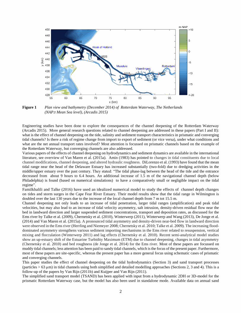
An example of a prismatic tidal channel with large water depths is the tidal Rotterdam Waterway in The Netherlands, which

is the artificial mouth of the river Rhine and has a length of about 30 km, see Figure 1. This tidal channel is briefly described

here, as field data from this case has been used for verification of the various models applied in this Part I. More information

related to mud is given in Part II. The water depth (below mean sea level) of the Waterway decreases stepwise from about 18

m at the mouth to about 11 m near the city of Rotterdam at about 30 km from the mouth and to 8 m more upstream. The tidal

range at the mouth is about 1.85 m during mean tidal conditions at present (2017). The annual-mean fresh water discharge

through the Waterway is about Qwaterway,50%=1310 m3/s (upstream river discharge at German border of Qupstream,50%= 2200 m3/s).

The bed of the Waterway channel sections is relatively flat (regular dredging) and consists of fine to medium sand (0.2-0.4

mm) with a gradually increasing percentage of mud from 5% at the mouth to 35% at about 20 km from the mouth. During the

past decades, the Rotterdam Waterway has undergone a process of constant deepening to accommodate larger vessels calling

at the ports of Rotterdam. Plans have been made by the Port Authorities for further deepening (from 15 m to 16.3 m between

km 1010 and 1030, see Figure 1) of some sections of the main navigation channel.

mailto:[email protected]




2

Figure 1 Plan view and bathymetry (December 2014) of Rotterdam Waterway, The Netherlands

(NAP Mean Sea level), (Arcadis 2015)

Engineering studies have been done to explore the consequences of the channel deepening of the Rotterdam Waterway

(Arcadis 2015). More general research questions related to channel deepening are addressed in these papers (Part I and II):

what is the effect of channel deepening on the tide, salinity and sediment transport characteristics in prismatic and converging

tidal channels? Is there a risk of regime change from import to export of sediment (or vice versa), under what conditions and

what are the net annual transport rates involved? Most attention is focussed on prismatic channels based on the example of

the Rotterdam Waterway, but converging channels are also addressed.

Various papers of the effects of channel deepening on hydrodynamics and sediment dynamics are available in the international

literature, see overview of Van Maren et al. (2015a). Amin (1983) has pointed to changes in tidal constituents due to local

channel modifications, channel deepening, and altered hydraulic roughness. DiLorenzo et al. (1993) have found that the mean

tidal range near the head of the Delaware Estuary has increased substantially (two-fold) due to dredging activities in the

middle/upper estuary over the past century. They stated: “The tidal phase-lag between the head of the tide and the entrance

decreased from about 9 hours to 6.4 hours. An additional increase of 1.5 m of the navigational channel depth (below

Philadelphia) is found (based on numerical simulations) to have a comparatively small or negligible impact on the tidal

regime”.

Familkhalili and Talke (2016) have used an idealized numerical model to study the effects of channel depth changes

on tides and storm surges in the Cape Fear River Estuary. Their model results show that the tidal range in Wilmington is

doubled over the last 130 years due to the increase of the local channel depth from 7 m tot 15.5 m.

Channel deepening not only leads to an increase of tidal penetration, larger tidal ranges (amplification) and peak tidal

velocities, but may also lead to an increase of tidal velocity asymmetry, salt intrusion, density-driven residual flow near the

bed in landward direction and larger suspended sediment concentrations, transport and deposition rates, as discussed for the

Ems river by Talke et al. (2009), Chernetsky et al. (2010), Winterwerp (2011), Winterwerp and Wang (2013), De Jonge et al.

(2014) and Van Maren et al. (2015a). A pronounced tidal asymmetry and density-driven near-bed flow in landward direction

were observed in the Ems river (Herrling and Niemeyer 2008; Chernetsky et al. 2010; Talke et al. 2009). The increasing flood-

dominated asymmetry strengthens various sediment importing mechanisms in the Ems river related to resuspension, vertical

mixing and flocculation (Winterwerp 2011) and lag effects (Chernetsky et al. 2010). Recent semi-analytical model studies

show an up-estuary shift of the Estuarine Turbidity Maximum (ETM) due to channel deepening, changes in tidal asymmetry

(Chernetsky et al. 2010) and bed roughness (de Jonge et al. 2014) for the Ems river. Most of these papers are focussed on

muddy tidal channels; less attention has been paid to sandy tidal channels, which is the focus of the present paper. Furthermore,

most of these papers are site-specific, whereas the present paper has a more general focus using schematic cases of prismatic

and converging channels.

This paper studies the effect of channel deepening on the tidal hydrodynamics (Section 3) and sand transport processes

(particles > 63 m) in tidal channels using both simplified and detailed modelling approaches (Sections 2, 3 and 4). This is a

follow-up of the papers by Van Rijn (2011b) and Kuijper and Van Rijn (2011).

The simplified sand transport model (TSAND) has been applied with input from a hydrodynamic 2DH or 3D-model for the

prismatic Rotterdam Waterway case, but the model has also been used in standalone mode. Available data on annual sand

3

dredging volumes (Arcadis 2015) of the prismatic Rotterdam Waterway has been used for overall verification of the computed

results (Section 4.1).

The proposed simplified model for sand transport in tidal flow (standalone mode or coupled to hydrodynamic models) is a

new development and can be used for quick evaluation of the most relevant parameters affecting channel deepening. Based

on this, the parameter range can be narrowed down substantially to reduce the number of detailed numerical model runs. The

standalone model has been used to produce a general graph of net tide-integrated sand transport rates as function of water

depth and river discharge for sand of 0.25 mm (Section 4.2). This general plot clearly shows the effect of channel deepening

on the import or export of sand at the mouth of a tidal channel with a tidal range of about 2 m. This provides both qualitative

and quantitative insights of channel deepening effects on sand transport processes. The plot can be used to make a first

assessment of the effects of channel deepening on the tide-integrated sand transport rates and hence on dredging volumes. In

Part II, a similar approach for mud transport (particles < 63 m) is presented.

Typical examples of muddy rivers with turbidity maxima (increased mud concentrations) in Europe are discussed in Part II:

tidal Elbe river in Germany; tidal Ems river in Germany; Loire river in France; Western Scheldt tidal estuary and Rotterdam

Waterway (Rhine mouth) in The Netherlands. A simplied mud transport model (TMUD) is described and applied in Part II.

2. Model description

2.1 Detailed models

Various detailed hydrodynamic and sediment transport models have been used by the authors. Herein, the leading detailed

model is the non-linear Delft3D-model for shallow waters, which has been applied in 3D and in 2DH-mode. The 3D-Flow

module solves the unsteady shallow-water equations in one (1DH), two (2DV or 2DH) or three dimensions (3D). The system

of equations consists of the horizontal momentum equations, the continuity equation, the salinity transport equations, and

various turbulence closure models. The vertical momentum equation is reduced to the hydrostatic pressure relation as vertical

accelerations are assumed to be small compared to the gravitational acceleration and are not taken into account. This makes

the 3D model suitable for predicting the flow in shallow seas, coastal areas, estuaries, lagoons, rivers, and lakes. The user

may choose whether to solve the hydrodynamic equations on a Cartesian rectangular, orthogonal curvilinear (boundary fitted),

spherical grid or flexible mesh grid. In three-dimensional simulations a boundary fitted (-coordinate) approach as well as a

fixed grid are available for the vertical grid direction. The 3D model has been used in combination with submodels for salinity

and sediment transport. Various simple sediment transport formulae and the detailed transport model for sand and mud (Van

Rijn 1984, 2007) have been implemented. The non-linear 2DH and 3D-models of the Delft-model system have been used and

verified extensively in numerous studies (Lesser et al. 2004, Van Rijn 2007, Van Rijn 2011a,b, Van Maren et al. 2015a,b,).

The 3D-hydrodynamic model of the Port Authority of Rotterdam has also been used. This hydrodynamic model is based on

the same equations as the Delft3D-model, but uses a different schematization with a much finer horizontal grid to better

include all geometric details of the Port of Rotterdam with all its docks at the expense of very large run times. This latter

model was carefully calibrated to represent the observed water levels (errors within 0.1 m) and the observed salinity

distribution (errors within 10% for salt intrusion length) along the Rotterdam Waterway (Arcadis 2015).

2.2. Simplified models

Simple approximations for tidal penetration, peak tidal velocities, tidal asymmetry, salinity-intrusion, density-driven

circulation velocities, and tidal sand transport in prismatic and converging models are used (Van Rijn 2011b). In the case of

converging channels, the width is represented by b=bo exp(-x/), with: b= channel width, bo=channel width at mouth, =

converging length scale. A tidal channel is almost prismatic for > 300 km (width reduction of about 65% over 300 km). Strongly

converging channels have < 30 km (width reduction of 65% over 30 km). Weakly converging channels for between 30 and

300 km.

2.2.1 Linear tidal model

The simplest way to study the effect of water depth and channel deepening on the tidal parameters along prismatic and

converging tidal channels is by using a linear tidal model. The classical solution of the linearized mass and momentum balance

equations for a prismatic channel of constant depth and width is well-known (Lorentz 1922, 1926; Dronkers 1964; Van Rijn

2011a,b). This solution for a prismatic channel represents an exponentially damped sinusoidal wave which dies out gradually

in a channel with an open end or is reflected in a channel with a closed landward end. In a frictionless system with depth ho

both the incoming and reflected wave have a phase speed of co= (gho)0.5 and have equal amplitudes resulting in a standing

wave with a virtual wave speed equal to infinity due to superposition of the incoming and reflected wave. Including (linear)

friction, the wave speed of each wave is smaller than the classical value co (damped co-oscillation). The linear approach can

also be used for exponentially converging channels, which has been explained and verified in detail in earlier work (Van Rijn

2011a,b).

4

It is noted that the linearized solution cannot deal with the various sources of non-linearity such as: quadratic friction, large

ratio of tidal amplitude and water depth, convective acceleration, variation of the water depth under the crest and trough,

effects of river discharges and effects of tidal flats causing differences in wave speed and hence wave deformation. Therefore,

the non-linear Delft3D-model (in 2DH-mode) has also been used for some cases.

Neglecting the convective acceleration term ( u u /x; very small in tidal channels; see Van Rijn 2011a,b), the equations of

continuity and motion for depth-averaged flow in a prismatic channel with a rectangular cross-section are:

b η Q ______ + ______ = 0 (1)

t x

1 Q g η Q Q ________ + ________

+ ____________ = 0 (2)

A t x C2 A2 R

in which: A = b ho = area of cross-section, b = surface width, ho = depth to MSL (mean sea level), R = hydraulic radius ( ho

if b>>ho), η = water level to mean sea level, Q= discharge= A u , u =cross-section-averaged velocity of the main channel,

see Figure 2, A= area of cross-section of main channel and C = Chézy-coefficient =5.75 g0.5log(12R/ks), ks= bed roughness

height of Nikuradse (1933).

The equations of continuity and momentum for a wide, prismatic channel with rectangular cross-section and constant mean

depth (h = ho+ ) can be linearized (Lorentz-method) by replacing the quadratic friction term by a linear term, as follows:

η ho u ______ + _________ = 0 (3)

t x

u g η

______ + _______ + m u = 0 (4)

t x

in which: u = cross-section-averaged velocity, u = amplitude of the tidal current velocity, m = linear friction coefficient =

(8g u )/(3πC2R), R= hydraulic radius (R ho for a very wide channel b>>ho). Very similar equations can be specified for a

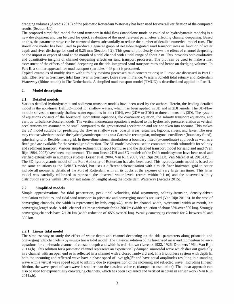
compound channel (Figure 2) with tidal flats (rectangular cross-sections of flats and main channel; Van Rijn 2011a).

Figure 2 Schematized cross-section of compound channel with main channel and tidal flats

In the case of a compound cross-section consisting of a main channel and tidal flats it may be assumed that the flow over the

tidal flats is of minor importance and only contributes to the tidal storage. The discharge is conveyed through the main channel.

This can to some extent be represented by using: co= (g heff)0.5 with: heff = Ac/bs = h hc with h = bc/bs; Ac= area of main

channel (=bchc), hc = depth of main channel (reduces to ho without flats), bc= width of main channel, bf= width of flats and bs=

bc+bf=surface width.

The transfer of momentum from the main flow to the flow over the tidal flats can be seen as additional drag exerted on the

main flow (by shear stresses in the side planes between the main channel and the tidal flats). This effect can be included to

ho

bchannel

HW= High Water

LW=Low Water

bflats

Amplitude MSL = Mean Sea Level

5

some extent by increasing the friction in the main channel slightly. If the hydraulic radius (R) is used to compute the friction

parameters (m and C) and the wave propagation depth (heff= R), the tidal wave propagation in a compound channel will be

similar to that in a rectangular channel with the same cross-section A.

The solution for a prismatic channel is an exponentially damped wave due to bottom friction, as follows:

x,t = η o [e

−x] [cos(t − kx)] (5a)

u x,t = u o [e −x ] cos(t − kx+) (5b)

u o= -( η o/ho) (/k) [cos] = -( η o/ho) c [cos] (5c)

with: = friction parameter, k = wave number, c= wave speed, = phase lead of velocity, H=2 η o = tidal range, tan = /k, x

= horizontal coordinate; positive in landward direction, u o= peak tidal velocity of linear model. The detailed solutions for

prismatic and converging channels are similar (Van Rijn 2011a,b). It is noted that the linear model is not very accurate for very

small water depths (ratio η o/ho should be <<1).

2.2.2 Simplified tidal sand transport model (TSAND-model)

Definitions

We have developed a simplified sand transport model for tidal flow to describe the transport of sand (TSAND). The simplified

approach is based on the detailed sediment transport formulations by Van Rijn (2007), which have been verified extensively.

The detailed sediment transport formulations have been implemented in the Delft3D-model.

The TSAND-model can be used in standalone mode or in post-processing mode (coupled to hydrodynamic model) to compute the

variation of the depth-integrated suspended sand transport and total transport (incl. bed-load transport) over the tidal cycle. It is

assumed that the fine sand concentrations are quickly adjusting to local flow conditions (no significant under or overloading).

The velocities and sand concentrations are computed as a function of z and t; z=height above bed and t=time (time step of 5 min).

The grid points over the depth (50 points) are distributed exponentially, as follows: z=a[h/a](k-1)/(N-1) with: a= reference height

above bed (input value), h=ho+= water depth, ho= depth between bed and mean sea level, = tidal water level, k= index number

of point k, N= total number of grid points. Used as a standalone model, the basic hydrodynamic parameters should be specified

by the user. Used as a post-processing model, the hydrodynamic input may come from a 1D, 2DH or 3D-model. TSAND can be

used for prismatic and converging channels.

Tidal water levels, flow and asymmetry

The tidal water level at each time t is represented, as:

flood,t = flood,max sin{(t-T)/Tflood)} for t < Tflood (6a)

flood,max = a (H/2) and Tflood= (ebb,max/H)T

ebb,t = ebb,max sin{(t-Tflood-T)/Tebb} for t > Tflood (6b)

ebb,max = H - flood,max and Tebb= (flood,max/H)T

with: H = flood,max + ebb,max = tidal range between the levels of HW and LW; a= asymmetry factor (input value a=1 tot 1.2 see

Figure 8, a=1 yields a symmetrical tide), T= tidal period (input value), T= phase shift (velocity is ahead of water level, input

value), Tflood= flood period, Tebb= ebb period. In standalone mode, only one representative tide of the neap-spring cycle is

considered (H, a, T specified as input by user); the tidal range H comes from the linear tidal model (Section 2.2.1).

The depth-averaged velocity at each time t is represented, as:

t = r + max,flood sin(t/Tflood) for t < Tflood (7a)

max,flood = a ( max)

t = r + max,ebb sin{(t-Tflood)/Tebb} for t > Tflood (7b)

max,ebb = -1/a ( max)

with: t=depth-averaged velocity at time t (m/s), r= net tide-averaged and depth-averaged velocity = Q/(b h), b= flow width

of channel (input value), h= water depth (input value), max== peak tidal velocity of sinusoidal tide (input).

u u uu uu u uu u

u uu

6

Equation (7) is used to describe the tidal motion of one single tide in the case that the model is used in standalone mode. An

asymmetrical tide can be generated, using the asymmetry factor a. Tidal flow in various type of channels has been studied to

determine the asymmetry factor a, (Section 3.3). If the sediment transport model is used as a post-processing model, the near-

bed velocity of the hydrodynamic model (1D, 2DH or 3D) is used as input.

The vertical distribution of the velocity at each time t is represented, as:

uz,t= urs,z + [ t/(-1+ln(h/zo))] ln(z/zo) (8)

with: urs,z= residual flow velocity due to horizontal salinity-induced density gradient based on Equation (9), z= level above bed

(m), h= = ho+t = water depth at time t (m), ho= tide-averaged water depth (m), t = tidal water level (m), t = depth-averaged

flow velocity at time t due to tide + steady river current (m/s), r= Q/(bh)= river velocity, zo= 0.033ks,c = zero-velocity level, ks,c

= current-related bed roughness (wave-current interaction is neglected).

The first part of Equation (8) represents the residual flow due to the density gradient. The depth-integration yields zero flow

velocity. The second part represents the tidal velocity profile and the river flow velocity profile due to fresh water discharge. The

vertical velocity distribution of tidal and river flow is represented by a logarithmic function.

Due to density-driven gravitational circulation, a tide-averaged residual flow is generated in a prismatic channel with tidal

flow from the seaside and fresh river water flow from the landside. The residual flow is landward near the bottom and seaward

near the water surface. Residual density-induced flow in a prismatic tidal channel can be determined from the tide-averaged

momentum equation. There are two main contributions: the free convection contribution arising from the density difference

between salt water and fresh water and the fresh water discharge contribution. The sips-mechanism related to tidal straining

(Section 1 of Part II, see also Burchard and Baumert 1998) which enhances the landward-directed near-bed flow is neglected.

Based on the tide-averaged equation of momentum (including eddy viscosity concept) and no net flow over the depth, the

residual (secondary) velocity profile related to density-driven flow can be derived (Hansen and Rattray 1965, Chatwin, 1976

and Prandle, 1985, 2004, 2009). Herein, a similar approach based on a constant vertical eddy viscosity concept is used,

resulting in (Van Rijn 2011a):

urs,z = Mho2 [− (1/6) (z/ho)3 + (1/2) (z/ho)2 − (1/4) (z/ho)] (9)

M = (g ho/E) (1/m) (m/x) = [g0.5 C/{ ( max+ r) ho}][(ho/fresh) (m/x)]

with: z= level above bed (m), ho= tide-averaged water depth (m), max= peak tidal velocity, r= Q/(bh)= river velocity, zo=

0.033ks,c = zero-velocity level, ks,c = current-related bed roughness of Nikuradse, M=salinity factor, E = u* ho= mixing coefficient

in near bed zone (constant), u*= (g0.5/C) (Umax+ r), C= Chézy-coefficient=5.75g0.5log(12h/ks,c), sea= density of sea water

(kg/m3), m/x= salinity-induced horizontal density gradient, m= depth-averaged and tide-averaged fluid density due to

salinity= fresh+ 0.77 S (kg/m3), fresh = fresh water density, S= salinity value (0 to 30 kg/m3), =coefficient (0.003 based on

calibration, see Part II). The maximum residual velocity of Equation (9) is approximately: us,max = −0.035Mho2 at about z/ho=

0.3.

Equation (9) is valid in the mouth region of a tidal channel where the vertical density profile is partially mixed over the depth.

The residual velocities are maximum in the near-bed region and show increasing residual velocities for increasing water depth

and increasing river discharge. The vertical mixing coefficient E (or ) is used as calibration parameter, which is discussed in

Part II based on measured and computed (3D-model) data of the Rotterdam Waterway.

Equation (9) is very similar to that of Hansen and Rattray (1965), Chatwin (1976) and Prandle (1985, 2004, 2009). The latter

derived for a partially-mixed estuary: us,max = Mho2 [− (1/6) (z/ho)3 + 0.27 (z/ho)2 − 0.037 (z/ho)-0.029], which yields us,max

−0.03Mho2 at about z = 0.1h. It is noted that the expression of Prandle yields a finite residual velocity value at z= 0 (at the

bed), whereas Euqation (9 ) yields a zero residual velocity at the bed.

The residual velocities generated by density differences due to strong horizontal sediment concentration gradients, which may

occur in the high turbidity zone (Talke et al., 2009), have been neglected. Hence, the model is less accurate when it is used in

standalone mode for the estuarine turbidity maximum (ETM) with relatively high horizontal sediment density variations.

u

uu

u u

u u

u

7

Sediment concentrations and transport

The sand concentrations are computed using a multi-fraction method (Van Rijn 2007). The multi-fraction method is based on

N=6 fractions (0.062-0.125 mm, 0.125-0.2 mm, 0.2-0.3 mm, 0.3-0.5 mm, 0.5-1 mm, 1-2 mm). The single fraction method is

obtained for N=1. The sand concentration profile at each time t is represented by an analytical expression, as:

ci=ca,i[((h-z)/z)(a/(h-a))]ZSi (10)

with: ci= concentration of fraction i (kg/m3), ZSi= suspension number of sediment fraction i (-).

The reference concentration ca of fraction i at reference level z=a is represented, as (Van Rijn 2007, Part II):

ca,i=0.015 ca (1-pmud) (di/a) (Ti)1.5 (D*,i)-0.3 (11)

with: ca= correction/scaling coefficient (default=1), d50= median particle diameter, a= input value,

D*,i= di[(s-1)g/2]0.333= dimensionless particle parameter,

Ti=[i(b/- I b,cr,d50)]/[(di/d50)b,cr,d50]= dimensionless bed-shear stress parameter of fraction i,

b,cr,d50= critical bed-shear stress of sand based on d50,

b/= cb,c+wb,w= effective bed-shear stress due to current and waves, s=s/= relative density,

=(1+pgravel)(1+pmud)3= factor representing effect of mud and gravel on the critical shear stress of sand,

i=(di/d50)0.25= roughness correction factor of fraction i,

i= (d50/di)0.5= hiding-exposure factor of fraction i (maximum 2 and minimum 0.5),

= kinematic viscosity coefficient, s= sediment density (input value), = fluid density,

pmud= fraction of mud (<0.063 mm) of top layer of bed (0 to 0.3),

pgravel= fraction of gravel (> 2 mm) of top layer of bed (0 to 0.1).

Equation (11) can be used for both sand (Part I), silt and mud (Part II).

The critical bed-shear stress of sand is represented by (Shields based on d50):

b,cr,sand= (s-) g d50 [0.3/D* + 0.055(1-e-0.02D*)] (12)

The critical bed-shear stress for erosion of mud (Part II) is an input parameter to deal with site-specific conditions (no general

relationship is available).

The bed-shear stresses at time t due to currents and waves are represented as:

b,c= (u*,c)2 with u*,c= uz /ln(30z/ks,c) (13)

b,w= 0.25 fw (Uw)2 (14)

with: = 0.4 and uz= flow velocity at z 0.1 h, Uw= (2/Tp)Aw=peak orbital velocity (linear wave theory), Aw= peak orbital

excursion, Tp= peak wave period, fw= exp(-6+5.2(Aw/ks,w)-0.19)= wave-related friction coefficient, = fluid density including

salinity effect; ks,c= current-related roughness, ks,w= wave-related roughness. The effect of surface waves are included to deal

with waves in the mouth of a tidal channel.

The effective bed-shear stresses at time t for sediment transport are represented as:

b,c/ = c b,c

(15)

b,w/= w b,w (16)

with: c=fc//fc= current-related efficiency factor, fc= 0.24/(log(12h/ks,c))2= current-related friction coefficient,

fc/=0.24/(log(12h/d90))2=grain-related friction coefficient, d90= grain size, w= 0.7/D*= wave-related efficiency factor

(w,min=0.14, w,max=0.35).

8

The suspension number ZS of sand is represented as:

ZSsand,i= wsand,i,o/(u*,cw) + 2.5(wsand,o/u*,cw)0.8(ca,sand/co)0.4 + (/fresh - 1)0.4 (17)

with: wsand,i,o= fall velocity of fraction i (based on formula Van Rijn 1993), =0.4, = 1+2(wsand,i/u*,cw)2= coefficient (max=1.5),

u*,cw=(u*,c2+u*,w

2)0.5= bed-shear velocity due to current and waves, u*,c= (b,c/)0.5= current-related bed-shear stress,

u*,w= (b,w/)0.5= wave-related bed-shear stress, ca= reference concentration, co=0.65=maximum bed concentration, = fluid

density including salinity effects, fresh = fluid density of fresh water (= 1000 kg/m3).

Equation (17) represents the effects of downward gravity settling, upward turbulence mixing (first term), empirical damping due

to vertical sediment concentration gradients (second term) and empirical damping due to vertical salinity gradients (third term),

(Winterwerp 2001; Van Rijn 1993). The damping due to vertical salinity/density gradients mainly occurs during the flood period

when the salt wedge penetrates landward. A larger ZS-value yields smaller concentrations.

The time lag effect of the suspended concentrations and suspended transport rate can be represented to some extent by applying

an exponential adjustment of the reference concentration at time t based on: dca/dt =-A(ca,t - ca,t,eq), resulting in (Van Rijn 2015):

ca,t=ca,t-t + dca (18)

ca,t=[1/(1 + A t)][ca,t-t + A t ca,eq,t]

with: t= time step (5 min), ca,t-t= suspended reference concentration at previous time (ca,i for multifraction method), ca,eq,t=

equilibrium reference concentration at time t,

A= c 0.05(1/h)(wsand,o/u*,cw)(1+2wsand,o/u*,cw)(1+Hs/h)2, Aminimum= 0.0005,

c= calibration coefficient (range 0.5 to 2; default =1).

The suspended transport qs can be computed by integration of the product of velocity and concentration over the water depth:

qs = oN ah (u c) dz with N= 6= number of fractions (summation over fractions and depth) (19)

The bed load transport (in kg/m/s) is computed by using a simplified expression (Van Rijn 2007).

The total load transport at each time t is computed as: qtot=qs+qb

The tide-integrated sediment transport rates are computed by integration over the tidal cycle.

Verification of sand transport model

The simplified approach presented here is based on the detailed sediment transport formulations by Van Rijn (1984, 1993, 2007,

2015), which have been verified extensively for river and tidal flow. The detailed formulations have been implemented in the

Delft3D modelling suite and the approach presented here is basically a simplified version of the detailed numerical model.

As the detailed sand transport model has been verified many times before (Van Rijn 1984, 1987, 2007; Lesser et al. 2004).

Herein, only one high-quality data set for tidal flow is considered. This case refers to measured sand concentrations and velocities

in a tidal channel of the Eastern Scheldt estuary in the southwest part of The Netherlands (Krammer, Station 2, 8 April 1987;

Voogt et al., 1991). The data set based on classical mechanical sampling instruments represents a wide range of velocities (1.4

to 1.9 m/s) and is a high-quality data set. The measured suspended transport has a relative error of about 30% (Voogt et al., 1991).

The water depths are in the range of 7 to 8 m. Water depth variations are due to tidal water level variations and the presence of

mega-ripples (with height of about 0.5 m). The bed material is sand with d50= 0.3 mm and d90=0.6 mm (six fractions: p1= 0.04;

p2=0.15, p3=0.35, p4=0.45, p5=0.01, p6=0).

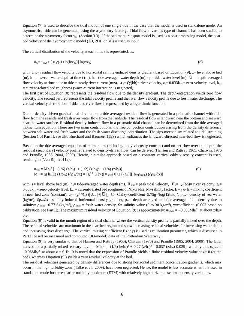
Model validation results are given in Figure 3 presenting the measured water depths, measured depth-mean velocities, measured

suspended transport rates and the computed suspended transport rates based on the single fraction and multi fraction methods

(TSAND-model) without any calibration. The bed roughness is taken to be ks= 0.4 m based on measured velocity data. The

depth-mean velocity increases from about 1.1 m/s to about 1.9 m/s at peak flow conditions resulting in a strong increase of the

suspended transport. The computed suspended transport rates of the multi fraction method are in good agreement with measured

values (all results within factor 2), although the computed model results are, on average, somewhat too small. The computed

suspended transport rates based on the single fraction method with dsus=d50= 0.3 mm are too small (factor 2). The single fraction

method produces good results if the suspended sediment size is calibrated to be dsus= 0.8d50 = 0.24 mm, which is in agreement

with earlier findings (Van Rijn 1984).

9

Figure 3 Measured and computed suspended sand transport in tidal channel Krammer, Eastern Scheldt, The Netherlands

(Voogt et al. 1991)

3. Effect of channel deepening on tidal parameters

To operate the TSAND-model in standalone mode for schematic and practical cases (Section 4.2), it is essential to have

knowledge of the peak tidal velocities in the mouth region (length<0.1 tidal wave length) and the velocity asymmetries

involved. We will therefore now study these parameters and the effects of channel deepening on these parameters by using

linear and non-linear models focussing on various schematic cases with varying water depth.

3.1 Tidal range and tidal penetration

In the case of a prismatic channel, the linear model solution is a damped tidal wave with a damping rate depending on the

water depth and the bed roughness. In the case of a converging tidal channel, the solution can be a damped tidal wave or an

amplified tidal wave depending on the converging length scale, the water depth and the bed roughness (Friedrichs 2010, Van

Rijn 2011a,b). It has been shown that the linear model works very well for a wide range of conditions (Western Scheldt

estuary (Netherlands), Hooghly estuary (India), Delware estuary (USA) and the Yangtze estuary in China (Van Rijn 2011a,b).

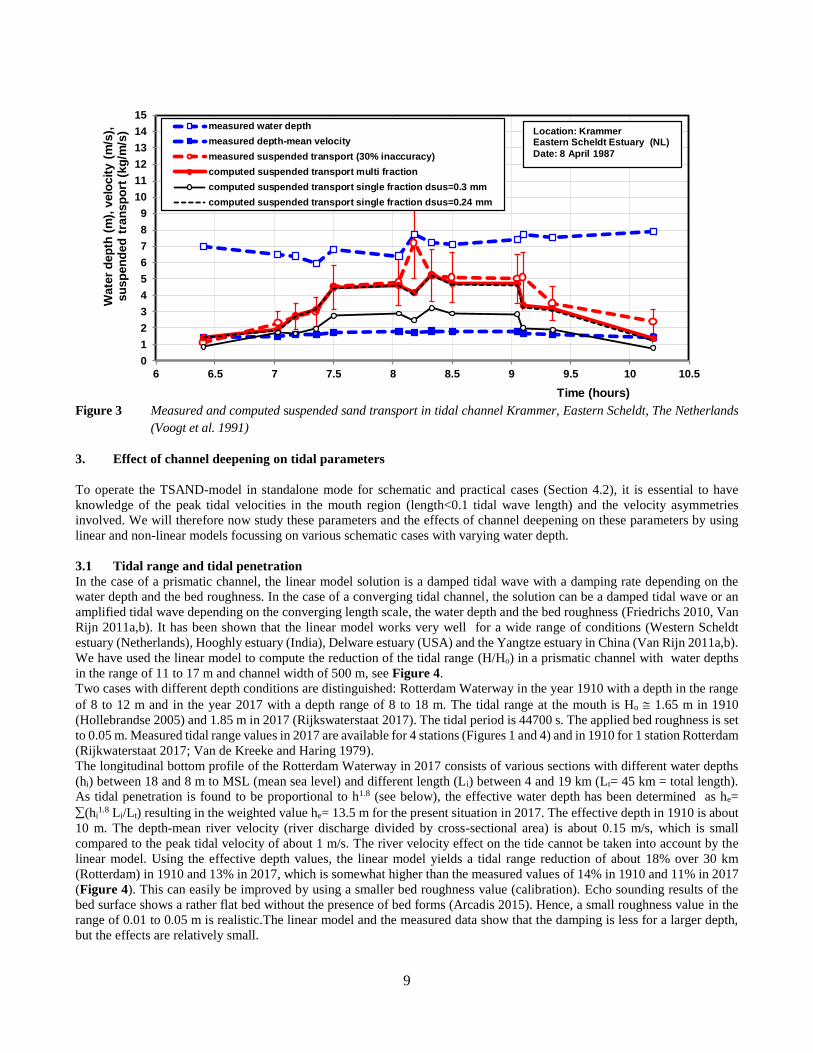
We have used the linear model to compute the reduction of the tidal range (H/Ho) in a prismatic channel with water depths

in the range of 11 to 17 m and channel width of 500 m, see Figure 4.

Two cases with different depth conditions are distinguished: Rotterdam Waterway in the year 1910 with a depth in the range

of 8 to 12 m and in the year 2017 with a depth range of 8 to 18 m. The tidal range at the mouth is Ho 1.65 m in 1910

(Hollebrandse 2005) and 1.85 m in 2017 (Rijkswaterstaat 2017). The tidal period is 44700 s. The applied bed roughness is set

to 0.05 m. Measured tidal range values in 2017 are available for 4 stations (Figures 1 and 4) and in 1910 for 1 station Rotterdam

(Rijkwaterstaat 2017; Van de Kreeke and Haring 1979).

The longitudinal bottom profile of the Rotterdam Waterway in 2017 consists of various sections with different water depths

(hi) between 18 and 8 m to MSL (mean sea level) and different length (Li) between 4 and 19 km (Lt= 45 km = total length).

As tidal penetration is found to be proportional to h1.8 (see below), the effective water depth has been determined as he=

(hi1.8 Li/Lt) resulting in the weighted value he= 13.5 m for the present situation in 2017. The effective depth in 1910 is about

10 m. The depth-mean river velocity (river discharge divided by cross-sectional area) is about 0.15 m/s, which is small

compared to the peak tidal velocity of about 1 m/s. The river velocity effect on the tide cannot be taken into account by the

linear model. Using the effective depth values, the linear model yields a tidal range reduction of about 18% over 30 km

(Rotterdam) in 1910 and 13% in 2017, which is somewhat higher than the measured values of 14% in 1910 and 11% in 2017

(Figure 4). This can easily be improved by using a smaller bed roughness value (calibration). Echo sounding results of the

bed surface shows a rather flat bed without the presence of bed forms (Arcadis 2015). Hence, a small roughness value in the

range of 0.01 to 0.05 m is realistic.The linear model and the measured data show that the damping is less for a larger depth,

but the effects are relatively small.

0

1

2

3

4

5

6

7

8

9

10

11

12

13

14

15

6 6.5 7 7.5 8 8.5 9 9.5 10 10.5

Wate

r d

ep

th (

m),

velo

cit

y (

m/s

),

su

sp

en

ded

tra

nsp

ort

(kg

/m/s

)

Time (hours)

measured water depth

measured depth-mean velocity

measured suspended transport (30% inaccuracy)

computed suspended transport multi fraction

computed suspended transport single fraction dsus=0.3 mm

computed suspended transport single fraction dsus=0.24 mm

Location: Krammer Eastern Scheldt Estuary (NL)

Date: 8 April 1987

10

Figure 4 Effect of water depth on the reduction of tidal range along the prismatic tidal channel of the Rotterdam

Waterway in 1910 and 2017 based on linear tidal model (ks=0.05 m)

Hereafter, the linear model is used to study the tidal penetration distance (Lp) as function of water depth, bed roughness and

the presence of tidal flats (compound prismatic channel) for a range of conditions, see Figure 5. The tidal penetration distance

is defined as the distance after which the tidal amplitude is smaller than 1% of that at the mouth. Water depth, bed roughness

and tidal flats are the most influencial parameters. It is clear that tidal penetration increases strongly for increasing water depth

(less friction); roughly Lp ho1.8 for ks= 0.01 m (see Figure 5) and Lp ho

1.5 for ks=0.1 m (see Figure 5) for situations with no

tidal flats. Tidal penetration increases for decreasing bed roughness ks (from 0.1 to 0.01 m). Tidal penetration is strongly

affected by the presence of tidal flats. The bed of the tidal flats is assumed to be between LW (low water level) and MSL

(mean sea level), see Figure 2. We have used two values of the width of the tidal flats: bflats=0.5 bchannel and bflats= bchannel. The

channel width is set to 500 m. As can be seen, the presence of tidal flats yields a significant reduction (more than 50%) of the

tidal penetration length. This underlines the importance of the tidal flats (see also Friedrichs and Aubrey 1988). Removal of

tidal flats leads to larger tidal penetration and associated salinity intrusion. In practice, the effect of tidal flats is much less as

tidal flats are usually only present in the outer part of the estuary. Tidal flats in the middle part of the estuary are often

reclaimed for commercial use.

Figure 5 Effect of water depth, bed roughness and tidal flats on tidal penetration for a prismatic tidal channel based

on linear tidal model

0.8

0.82

0.84

0.86

0.88

0.9

0.92

0.94

0.96

0.98

1

0 5000 10000 15000 20000 25000 30000 35000

Rela

tive t

idal

ran

ge H

/Ho

(-)

Distance from mouth (m)

Computed h=13 m

Computed h=15 m

Computed h=17 m

Computed h= 11 m

Measured 2017

Measured 1910

2017

1910

Hook of Holland Maassluis Vlaardingen Rotterdam

0

100

200

300

400

500

600

700

800

900

0 1 2 3 4 5 6 7 8 9 10 11 12 13 14 15 16

Tid

al

pe

ne

tra

tio

n le

ng

th (

km

)

Water depth (m)

ks=0.01 m, no tidal flats

ks=0.1 m, no tidal flats

ks=0.1 m, with tidal flats (b-flats= 0.5 b-channel)

ks=0.1 m, with tidal flats (b-flats= b-channel)

Tidal range at mouth= 2 m

11

3.2 Peak tidal velocity at mouth

The magnitude and direction of tidal sand transport in the mouth region strongly depends on the peak velocities of the tidal

system in that region and are discussed in this section. The horizontal distribution of the peak tidal velocities along the tidal

channel beyond the mouth region is discussed in Section 3.4.

We have used the linear model and non-linear models to compute the peak tidal velocity at the mouth of various tidal channels

and the phase shift between the vertical and horizontal tides. The peak tidal velocity at the mouth based on the linear model

primarily depends on the type of channel (prismatic or converging), the tidal range, the water depth and the bed roughness,

see Figure 6 for the linear model results and Figure 7 for both linear and non-linear models. The converging case is a strongly

converging tidal channel with a length of 60 km (<< tidal wave length) and a mouth width of 25 km reducing (exponentially)

to about 2 km at 60 km (resembling the Western Scheldt, The Netherlands).

In the case of prismatic channels, the peak velocity at the mouth increases from about 0.8 m/s at a tidal range of 2 m to about

2 m/s at a tidal range of 8 m based on Equation (5c). The effect of the water depth (between 10 and 20 m) is marginal for

prismatic channels; the peak velocity is slightly smaller for a larger depth. A smaller bed roughness of ks= 0.01 m (factor 5

smaller) leads to somewhat larger velocities (about 5%). A larger bed roughness of ks= 0.25 m (factor 5) leads to somewhat

smaller velocities (about 7%). The phase lead between the horizontal and vertical tide in prismatic channels decreases from

about 1.2 hours to 0.7 hours for increasing water depths between 5 and 15 m (not shown). The phase lead is almost zero for a

depth of 50 m. In a prismatic channel, the phase lead of the linear model only depends on the bottom friction and is fairly

accurate.

In the case of a strongly converging channel with a mouth width of 25 km reducing (exponentially) to about 2 km at 60 km

from the mouth, the peak velocities at the mouth are much smaller compared to those in prismatic channels. The effect of the

water depth is much stronger. Increasing the water depth from 10 m to 20 m leads to a velocity decrease of about 40%. In a

converging channel, the predicted phase lead of the linear model is less accurate as it depends on bottom friction and on the

converging length scale, which introduces additional schematization errors (Van Rijn 2011a,b).

A comparison of linear and non-linear model results is given in Figure 7, which shows the peak tidal velocity as function of

the water depth for a constant tidal range of 4.2 m (about the middle of the tidal range interval of Figure 6). The peak velocity

of the non-linear 2DH-model represents the average value of the peak flood and ebb values. The computed results of the linear

model and the non-linear 2DH-Delft model for a tidal range of 4.2 m are fairly similar. The linear model, although strictly

valid for η o<<ho) does surprisingly well for shallow depths ( η o/ho 0.3-0.4).

Figure 6 Effect of water depth and tidal range on the peak tidal velocity at the mouth for prismatic and converging

channels based on linear model (bed roughness= 0.05 m)

The relationship between the peak tidal velocity at the mouth and the water depth in prismatic channels can be determined

analytically using Equation (5c) of the linear model. Based on sensitivity computations using the linear model, the wave speed c

in water depth between 5 and 20 m is roughly proportional to cho0.7 and the phase lead (cos) is proportional to cos() ho

0.1.

The phase lead is about 1.5 hours for a very shallow prismatic channel (relatively large friction) and about zero for a very deep

channel (almost no friction). The value of cos() varies very weakly between 0.8 and 1. Given these results, the peak tidal

0

0.2

0.4

0.6

0.8

1

1.2

1.4

1.6

1.8

2

2.2

2.4

2.6

2.8

3

0 1 2 3 4 5 6 7 8 9

Pe

ak

tid

al

ve

loc

ity

at m

ou

th (

m/s

)

Tidal range (m)

Prismatic; water depth= 10 m (linear)



Converging; water depth= 10 m (linear)



Prismatic channels

Converging channels

12

velocity (Equation 5c) at the mouth of a prismatic channel without flats varies roughly as: u o ho-0.2 yielding a weakly

decreasing curve for increasing channel depths, as shown in (Figure 7).

Thus, channel deepening has a very marginal effect on the peak tidal velocity in a relatively wide prismatic channel. In a

strongly converging tidal channel, the peak tidal velocity reduces by about 30% if the water depth increases (factor 3) from 5

to 15 m. Other configurations can be easily explored by the analytical linear model equations.

Figure 7 Effect of water depth on the peak tidal velocity at the mouth for prismatic and converging channels based on

linear and non-linear 2DH Delft-model (tidal range= 4.2 m; bed roughness= 0.05 m)

3.3 Tidal asymmetry at the mouth

The analytical solutions of the linearized equations of continuity and momentum presented above do not express the non-linear

effects. All non-linear terms ( u u /x; ( u )/x and u2) have been neglected or linearized. Thus, the wave speed is constant

and the peak flood and ebb velocities are equal (no asymmetry).

Friedrichs and Aubrey (1988) have shown for a short estuary without upstream river flow that the velocity asymmetry depends

on the relative tidal amplitude ( η o/ho) and the ratio Vs/Vc with η o= tidal amplitude, ho = water depth to mean sea level, Vs=

intertidal water volume between HW and LW above the flats and Vc=water volume in main channel below mean sea level. A

ratio Vs/Vc 0 means the presence of a channel without tidal flats resulting in flood dominance (a= u flood/ u ebb > 1). Ebb

dominance can occur if the propagation of the tide during flood is slowed down sufficiently by the water mass above the tidal

flats. During ebb, the flats are dry and the tide propagates through the main channel at a smaller water depth with larger flow

velocities resulting in ebb dominance. It is shown that ebb-dominant sand transport prevails at the mouth of shallow estuaries

for η o/ho < 0.3 with Vs/Vc > 0.3, which cover many small-scale estuaries in the USA. Flood dominance prevails for all

conditions without flats. Thus, flood-dominance occurs in shallow, narrow channels and ebb-dominance in deeper channels

with flats. Hence, shallow channels tend become shallower due to sediment import (flood dominance) and deeper channels

tend to become deeper due to sediment export (ebb dominance) for tidal channels without river flow (no river flushing). In

practice, the morphodynamic behaviour also depends on the location of the channel within the estuary. Some flood or ebb-

dominated channels may show (quasi) morphodynamic equilibrium due to sediment supply from adjacent channels.

Furthermore, relatively short tidal inlet channels may behave in a different way than longer estuary channels.

We studied the velocity asymmetry effects in the mouth region of tidal channels based on computed data available in the

literature and new additional Delft3D model simulations. The focus is to obtain a simple relationship between tidal velocity

asymmetry (a= u flood/ u ebb) and the relative tidal amplitude ( η o/ho), which can be used if the TSAND-model is used in

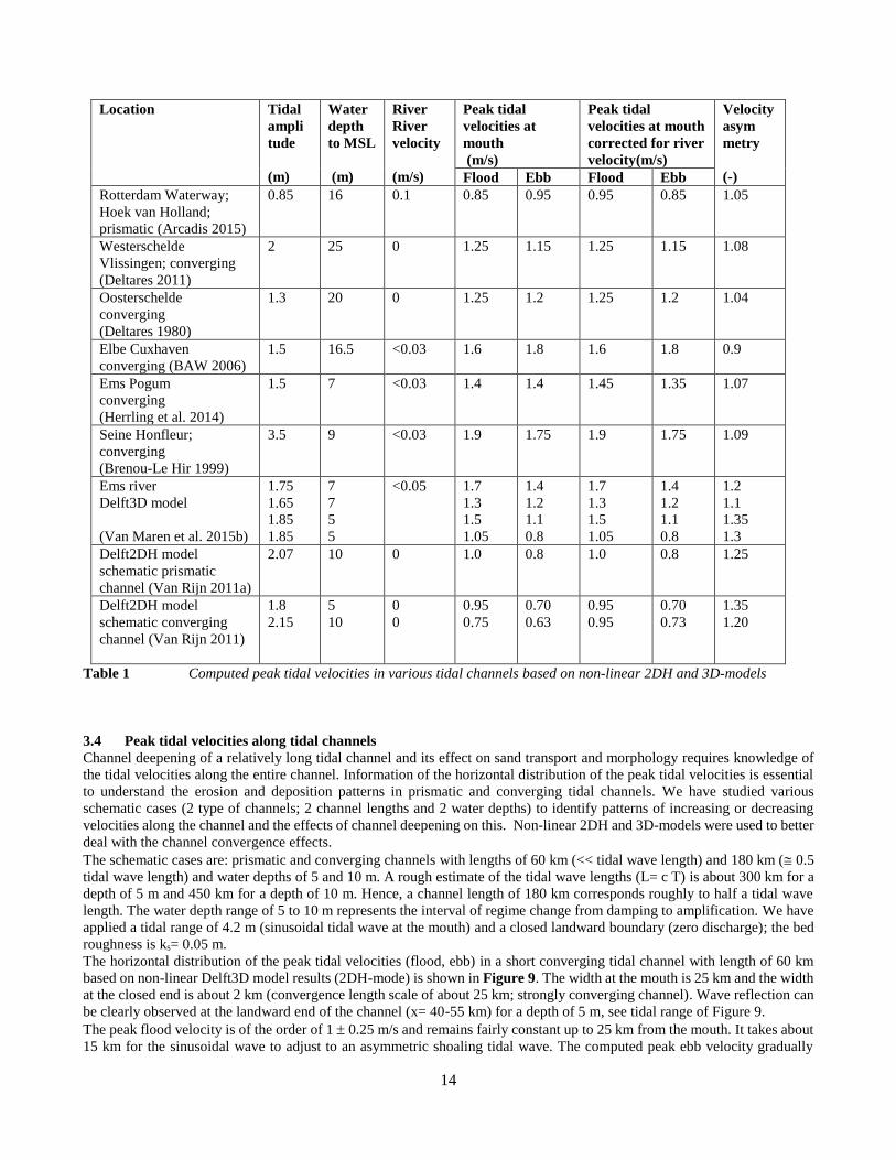
standalone mode (feasibility studies/quick-scan studies), see Figure 8 and Table 1 with all data sources included. The data

refer to computed peak tidal velocities in the mouth of various tidal channel sections of major European rivers based on non-

linear 2DH and 3D-model results. For almost all natural tidal rivers/channels the velocity asymmetry is > 1 (flood dominance),

but the asymmetry factor remains small between 1 and 1.2. The model simulations for the Ems river (Van Maren et al. 2015b)

are based on two Manning-coefficients (relatively smooth: n=0.01 or C= 130 m0.5/s; relatively rough: n=0.02 or C= 65 m0.5/s).

0

0.2

0.4

0.6

0.8

1

1.2

1.4

1.6

1.8

2

2.2

2.4

2.6

2.8

3

0 1 2 3 4 5 6 7 8 9 10 11 12 13 14 15 16 17 18 19 20

Pe

ak

tid

al

ve

loc

ity

at m

ou

th (

m/s

)

Water depth (m)

Prismatic Ho=4.2 m: Peak velocity; non-linear model

Prismatic Ho=4.2 m: Peak velocity; linear model

Converging Ho=4.2 m: Peak velocity; linear model

Converging Ho=4.2 m: Peak velocity; non-linear model

Prismatic Linear

Non-linearConverging

Non-linear

Linear

13

The upper error bar of the Ems river data (Figure 8) refers to smooth bed conditions and the lower error bar refers to rough

bed conditions. The velocity asymmetry is about 10% larger for smooth bed conditions. The model results of Herrling et al.

(2014) for the Ems-river show a somewhat smaller asymmetry value.

The Elbe tidal channel at Cuxhaven (mouth region) is an exception with a velocity asymmetry factor of 0.9 (Figure 8), which

is most likely related to the presence of wide tidal flats (5 to 10 km wide) in the mouth region. The water volume above the

flats drains through the main channel during ebb with relatively small water depths resulting in a strong increase of the peak

tidal velocity during ebb. The ratio Vs/Vc is about 1 and η o/ho is about 0.1 which yields ebb-dominance based on the results

of Friedrichs and Aubrey (1988).

Some results of the linear model are also shown in Figure 8. A first order estimation of the tidal asymmetry can be obtained by

using the linear model with the same settings at high water and at low water. The tidal asymmetry can be expressed as

A=cmax/cmin with cmax= wave speed at high water and cmin= wave speed at low water. As the peak tidal velocity is proportional

to the wave speed , see Equation (5c), it follows that A= cmax/cmin u flood/ u ebb. Very reasonable results can be obtained by

defining an effective high water depth and low water depth as hmax ho+0.5 η o and hmin ho-0.5 η o. The linear model has also

been applied for a compound channel with a main channel (bc=500 m; ks=0.1 m) and tidal flats (see Figure 2) with Vs/Vc in

the range of 0.2 to 0.05, yielding an asymmetry factor between 0.85 and 1 (ebb dominance) for bflats/bchannel= 1. The asymmetry

is smallest (0.85) for a deep main channel. The asymmetry is about 0.75 for bflats/bchannel= 4. The asymmetry factor approaches

1 for a shallow main channel with tidal flats. The flood-related asymmetry for prismatic and converging channels without

large-scale tidal flats (trend curve of Figure 8) can be represented by the following fit: a=1+( η o/ho)1.5. This latter expression

(goodness of fit r2 0.4) is used in the standalone TSAND-model for the computation of net tide-integrated sand transport

rates (Section 4.2). Available field data sets should be studied to confirm the proposed velocity asymmetry relationship, which

is mainly based on model data.

Figure 8 Effect of relative water depth (ratio of tidal amplitude and water depth) on tidal velocity asymmetry in the

mouth region of prismatic and converging tidal channels based on model results

0

0.1

0.2

0.3

0.4

0.5

0.6

0.7

0.8

0.9

1

1.1

1.2

1.3

1.4

1.5

1.6

0 0.05 0.1 0.15 0.2 0.25 0.3 0.35 0.4 0.45 0.5

Tid

al v

elo

cit

y a

sy

mm

etr

y facto

r (-

)

Ratio of tidal amplitude and water depth (-)

Delft 2DH model for prismatic channel (Van Rijn 2011)

Delft 2DH model for strongly converging channel (Van Rijn 2011)

Eastern Scheldt mouth converging channel (Deltares 1980)

Elbe mouth converging channel with flats (BAW 2006)

Western Scheldt mouth converging channel (Deltares 2011)

Rotterdam Waterway mouth prismatic channel (Arcadis 2015)

Ems mouth converging channel (Herrling et al 2014)

Seine mouth converging channel (Brenou-LeHir 1999)

Delft3D-model Ems river (Pogum, Terborg), (Van Maren 2015)

Linear model for prismatic channels

Linear model prismatic channels with tidal flats

Trendcurve

14

Location Tidal

ampli

tude

(m)

Water

depth

to MSL

(m)

River

River

velocity

(m/s)

Peak tidal

velocities at

mouth

(m/s)

Peak tidal

velocities at mouth

corrected for river

velocity(m/s)

Velocity

asym

metry

(-) Flood Ebb Flood Ebb

Rotterdam Waterway;

Hoek van Holland;

prismatic (Arcadis 2015)

0.85 16 0.1 0.85 0.95 0.95 0.85 1.05

Westerschelde

Vlissingen; converging

(Deltares 2011)

2 25 0 1.25 1.15 1.25 1.15 1.08

Oosterschelde

converging

(Deltares 1980)

1.3 20 0 1.25 1.2 1.25 1.2 1.04

Elbe Cuxhaven

converging (BAW 2006)

1.5 16.5 <0.03 1.6 1.8 1.6 1.8 0.9

Ems Pogum

converging

(Herrling et al. 2014)

1.5 7 <0.03 1.4 1.4 1.45 1.35 1.07

Seine Honfleur;

converging

(Brenou-Le Hir 1999)

3.5 9 <0.03 1.9 1.75 1.9 1.75 1.09

Ems river

Delft3D model

(Van Maren et al. 2015b)

1.75

1.65

1.85

1.85

7

7

5

5

<0.05 1.7

1.3

1.5

1.05

1.4

1.2

1.1

0.8

1.7

1.3

1.5

1.05

1.4

1.2

1.1

0.8

1.2

1.1

1.35

1.3

Delft2DH model

schematic prismatic

channel (Van Rijn 2011a)

2.07 10 0 1.0 0.8 1.0 0.8 1.25

Delft2DH model

schematic converging

channel (Van Rijn 2011)

1.8

2.15

5

10

0

0

0.95

0.75

0.70

0.63

0.95

0.95

0.70

0.73

1.35

1.20

Table 1 Computed peak tidal velocities in various tidal channels based on non-linear 2DH and 3D-models

3.4 Peak tidal velocities along tidal channels

Channel deepening of a relatively long tidal channel and its effect on sand transport and morphology requires knowledge of

the tidal velocities along the entire channel. Information of the horizontal distribution of the peak tidal velocities is essential

to understand the erosion and deposition patterns in prismatic and converging tidal channels. We have studied various

schematic cases (2 type of channels; 2 channel lengths and 2 water depths) to identify patterns of increasing or decreasing

velocities along the channel and the effects of channel deepening on this. Non-linear 2DH and 3D-models were used to better

deal with the channel convergence effects.

The schematic cases are: prismatic and converging channels with lengths of 60 km (<< tidal wave length) and 180 km ( 0.5

tidal wave length) and water depths of 5 and 10 m. A rough estimate of the tidal wave lengths (L= c T) is about 300 km for a

depth of 5 m and 450 km for a depth of 10 m. Hence, a channel length of 180 km corresponds roughly to half a tidal wave

length. The water depth range of 5 to 10 m represents the interval of regime change from damping to amplification. We have

applied a tidal range of 4.2 m (sinusoidal tidal wave at the mouth) and a closed landward boundary (zero discharge); the bed

roughness is ks= 0.05 m.

The horizontal distribution of the peak tidal velocities (flood, ebb) in a short converging tidal channel with length of 60 km

based on non-linear Delft3D model results (2DH-mode) is shown in Figure 9. The width at the mouth is 25 km and the width

at the closed end is about 2 km (convergence length scale of about 25 km; strongly converging channel). Wave reflection can

be clearly observed at the landward end of the channel (x= 40-55 km) for a depth of 5 m, see tidal range of Figure 9.

The peak flood velocity is of the order of 1 0.25 m/s and remains fairly constant up to 25 km from the mouth. It takes about

15 km for the sinusoidal wave to adjust to an asymmetric shoaling tidal wave. The computed peak ebb velocity gradually

15

decreases in landward direction. If the water depth is 10 m, the tidal range is amplified but the computed peak flood velocity

remains fairly constant at a value of 0.75 m/s up to 25 km from the mouth and decreases gradually after that. If the water

depth is 5 m and tidal damping is dominant, the peak tidal velocity decreases in landward direction of the converging channel

(x>30 km).

Figure 9 also shows computed peak velocities (mean of 2 computations) in the converging Ems river in Germany based on

the Delft3D model simulations with Manning coefficient n= 0.01 to 0.02 (Chézy =h1/6/n 130 to 65 m0.5/s), bathymetry of

2005; depths of 5 to 7 m (Van Maren et al. 2015b). A weir is present at Herbrum (15 km upstream of Papenburg; 85 km from

mouth) where the measured discharge rate is used as landward boundary condition. The tidal range (at spring tide) shows an

increase from about Ho= 2.8 m at the model boundary Emshorn to about 3.1 m in Knock (20 km), about 3.4 m in Pogum (35

km), to about 3.6 m in Papenburg at 70 km. Hence, the tide is stongly amplified due to geometry effects and resonance effects

(upstream weir). The computed peak tidal velocities are gradually decreasing from Station Pogum to Papenburg (Van Maren

et al., 2015b). The peak velocities in the section Knock to Pogum (20-35 km) of the Ems river are relatively large (up to 1.5

m/s) due to the presence of a long funnel type training wall with groins (transition from estuary to river). The computed peak

tidal velocities in the river mouth section between 35 and 60 km show a slightly decreasing trend. These qualitative trends

have also been found by Chernetsky et al. 2010 for the Ems river.

Figure 9 Effect of water depth on tidal range (upper) and peak flood and ebb velocities (lower) in short converging

channels based on non-linear 2DH and 3D-models

Similar computations have been made for a long converging channel of 180 km (schematic case), see Figure 10. The flow

width of the converging channel decreases from 25000 m at the mouth to 10 m at the closed end (strongly converging channel

with convergence length scale of about 25 km). Tidal damping is present in the converging channel with water depth of 5 m;

the tidal range decreases from 4.2 m at the mouth to about 3 m at the end. Wave reflection is present at the end of the channel

(150-180 km) where the tidal range is relatively large (not shown) for both depths (5 and 10 m). The peak flood velocity near

0

0.2

0.4

0.6

0.8

1

1.2

1.4

1.6

1.8

2

2.2

2.4

0 5 10 15 20 25 30 35 40 45 50 55 60 65 70

Pe

ak tid

al v

elo

cit

y (m

/s)

Distance along channel from mouth/seaward boundary(km)

Peak flood velocity, h= 5 m

Peak ebb velocity, h=5 m

Peak flood velocity, h=10 m

Peak ebb velocity, h=10 m

Peak flood velocity Ems, h=5 to 7 m

Peak ebb velocity Ems, h=5 to 7 m

0

1

2

3

4

5

6

0 5 10 15 20 25 30 35 40 45 50 55 60 65 70

Tid

al

ran

ge

(m

)


Tidal range; h=10 m

Tidal range; h= 5 m

Tidal range EMS; h= 5 to 7 m (springtide)

16

the mouth (< 25 km) remains fairly constant at 0.9 0.2 m/s. The peak ebb velocity is somewhat smaller (not shown). Strong

tidal amplification of the tidal range is present for a converging channel with h= 10 m; the tidal range increases from 4.2 m at

the mouth to about 9 m at the end. The peak flood velocity gradually increases from 0.8 m/s at the mouth to 1.4 m/s near the

end. Similarly the peak ebb velocities increase from about 0.8 m/s at the mouth to about 1.25 m/s near the end (not shown).

Hence, the peak tidal velocities are increasing in a strongly converging tidal channel (strong amplification) with a water depth

of 10 m, particularly beyond the mouth region (> 30 km). It is noted that a convergent channel reducing to a width of about

10 m over a distance of 180 km is not very realistic in practice. It is more likely that after a convergent section, the river has

a constant width. This case, which has also been studied (Van Rijn 2011a), shows that damping due to bottom friction is the

dominant process in the constant width section.

In the prismatic channel with a length of 180 km, the peak tidal velocity always decreases in landward direction due to the

tidal damping effect. The decrease of the velocity is less for a larger water depth (less damping), as shown in Figure 10.

The effect of channel deepening on the peak tidal velocities in the prismatic Rotterdam Waterway is presented in Figure 11

based on results of the non-linear 3D-model including salinity. The depth-averaged peak flood current velocity is about 0.8

m/s in the wider outer section and increases to about 1.2 m/s in the narrower section (km 1030-1015). The velocity is largest

in the opening of the Maeslant barrier where the river width is smallest. The velocity reduces to about 0.8 m/s in the upstream

river sections.

Figure 11 makes clear that the further deepening of an already deep channel from 15 m to 16.3 m such as the Rotterdam

Waterway (from 15 m to 16.3 m) only has a marginal effect on the depth-averaged velocities (lowest panel of Figure 11).

This was also concluded by DiLorenzo et al. (1993) for the Delaware estuary (USA). However, the 3D-model results of the

Rotterdam Waterway show that the near-bed flood velocities are most significantly affected (variation of 20%) in the section

km 1020-1010 with the salinity front, which has serious consequences for the sand transport and deposition processes in that

region.

Figure 10 Effect of water depth on tidal range (upper) and peak flood velocities (lower) in long, converging/prismatic

channels (180 km) based on non-linear 2DH-model

0

4

8

12

16

20

24

28

32

0

1

2

3

4

5

6

7

8

0 10 20 30 40 50 60 70 80 90 100

Flo

w w

idth

(km

)

Tid

al

ran

ge (

m)

(m)


Tidal range, Converging: h= 10 m

Tidal range, Converging: h= 5 m

Tidal range, Prismatic: h= 10 m

Tidal range, Prismatic: h= 5 m

Flow width: Converging Channel

0

0.2

0.4

0.6

0.8

1

1.2

1.4

0 10 20 30 40 50 60 70 80 90 100

Peak t

idal v

elo

cit

y (

m/s

)


Converging, h=10 m

Converging, h= 5 m

Prismatic, h=10 m

Prismatic, h= 5 m

Peak tidal flood velocity

17

Summarizing, channel deepening in a prismatic channel leads to less tidal damping an hence to slightly larger tidal ranges.

The peak tidal velocity in a deepened prismatic channel remains fairly constant in the mouth region. Further deepening of an

already deep channel only has a marginal effect on the depth-averaged velocities. However, near-bed velocities may be

significantly (about 20%) affected in the salinity front zone.

Channel deepening from a small depth of about 5 m to a larger depth of 10 m in a strongly converging channel leads to a

regime shift from tidal damping to tidal amplification with much larger tidal ranges along the channel. Similar results have

been found by DiLorenzo et al. (1993), Chernetsky et al. (2010), Winterwerp (2011), Van Maren et al. (2015a,b), Familkhallili

and Talke (2016). The peak tidal velocities in the mouth region (< 25 km) of a converging channel may decrease by about

20% due to channel deepening. The present cases studied using linear and non-linear models do not show any significant

increase of the peak tidal velocities in the mouth region due to channel deepening in converging channels.

Our results substantiate earlier ideas of Friedrichs (2010), who has observed that many prismatic and converging tidal channels

with an erodible sediment bed have a rather constant peak tidal velocity in the mouth region and are typified as "equilibrium"

to "near-equilibrium" channels.

In the following section 4, it is studied how the tide-integrated sand transport processes are affected by channel deepening in

the prismatic tidal channel of the Rotterdam Waterway. As a result, the depth of a near-equilibrium tidal channel with an

erodible sediment bed is more precisely defined.

Figure 11 Effect of water depth on peak flood velocities along Rotterdam Waterway for present and deepened channel

(North Sea at km 1035) based on non-linear 3D model; tidal range Ho=1.85 m and Qwaterway,50%=1310 m3/s

(QLobith upstream, 50%=2200 m3/s); (Arcadis 2015)

4. Effect of channel deepening on tide-integrated sand transport along tidal channels

Hereafter in Section 4.1, the effect of channel deepening on the sand transport processes in the Roterdam Waterway is studied

using a detailed 3D-model in combination with the TSAND-model. The detailed 3D-model of the Rotterdam Waterway is

based on very small grid cells resulting in relatively large run times. To be able to do many sensitivity sand transport runs,

the 3D-model output of the near-bed velocity and salinity values along the channel axis during the neap-spring tidal cycle is

used as input for the TSAND-model. Many runs were made to determine mean values including the variation range of the net

sand transport rates along the channel axis, which could not have been done by using the 3D model including the advection-

diffusion equation of the sand concentrations and transport rates. First, it is shown that the TSAND-model produces sand

transport rates which are in good agreement (justification) with those of the detailed Delft3D-model. After that, the results of

some sensitivity runs varying the most influencial parameters are shown and discussed.

In Section 4.2, the TSAND-model is used in standalone mode with hydrodynamic input results from Section 3 to compute the

net tide-integrated sand transport rates for a wide range of water depths and fresh water discharges in order to explain the

change from sand export to import and the concept of “equilibrium” depth of tidal channels.

Finally in Section 4.3 the results are discussed.

18

4.1 Channel deepening of Roterdam Waterway; 3D-model with TSAND

We have validated the TSAND-model in post-processing mode (with hydrodynamic input of the 3D model) by comparing

the sand transport rates of the 3D-model (10 vertical grid points) with and without the TSAND-model. The channel bed

consists of sand with d50 = 0.25 mm and mud with varying percentages of 5% at the mouth to 35% near Rotterdam. Local

patches of gravel are present as relict features of local bed stabilization measures. The d50 of the sand fraction is varied in the

range of 0.15 to 0.35 mm based on observed values.

The boundary conditions are a spring-neap tidal cycle (tidal range of about H=2 m) in combination with a fresh water discharge

in the Waterway of Qwaterway,50%=1310 m3/s. Using default parameter settings, the TSAND-model with 50 grid points over the

water depth and near-bed velocity input of the 3D-model (including salinity effects) produces very similar sand transport

results as that of the 3D-model with advection-diffusion equation for sand concentrations, see Figure 12. The net tide-

integrated sand transport is obtained by integrating the instantaneous sand transport rates over the spring-neap cycle and

dividing by the number of tides within the cycle and is expressed in ton/m/tide. The differences between the 3D-model and

the TSAND-model are largest (maximum 55%) in the mouth region (km 1030-1027). These deviations are mainly caused by

the difference in the number of vertical grid points used in both models (10 points in 3D-model and 50 points in TSAND-

model).

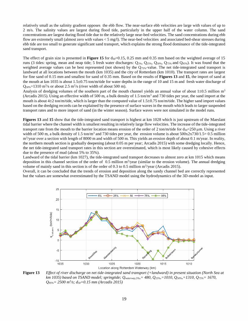
Many TSAND-postprocessing runs were done varying the most important sand transport parameters and model coefficients

(Arcadis 2015). The focus parameter is the net tide-integrated sand transport rate, which is shown in Figure 13 for springtide

in combination with five fresh water discharges and d50 = 0.15 mm.

Figure 12 Comparison of net tide-integrated sand transport (+ landward) along the Rotterdam Waterway (North Sea at

km 1035) based on 3D model; neap-spring cycle; river discharge Qwaterway,50% = 1310 m3/s; d50= 0.25 mm;

(Arcadis 2015)

The tide-integrated sand transport rate is landward-directed at all locations except for the largest fresh water discharge of

Q95%= 2500 m3/s in the Waterway. In the latter case, the transport rate is in landward direction between km 1035 and 1020

and seaward beyond km 1020. It is noted that the net sand transport rate upstream in the region of Rotterdam (x < 1010 km)

is almost zero due to the presence of relatively small depth-averaged flow velocities during the tidal cycle (< 0.6 m/s), even

at large fresh water discharges. The sand transport far upstream in the almost steady river flow section is about 10 to 20

ton/m/tide. Sand is mined/dredged in the depositional area at the transition between the tide-dominated and river-dominated

sections.

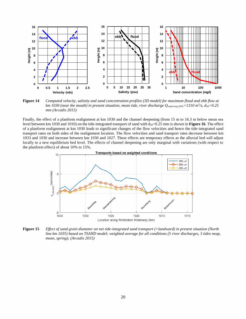
The dominant effect of the flood velocities on the net tide-integrated sand transport rates can be explained by Figure 14,

which shows the velocity, salinity and sand concentration profiles during peak flood and ebb flow at km 1030 during mean

tide, fresh water discharge Qwaterway,50%= 1310 m3/s and d50=0.25 mm. The velocity and salinity profiles are from the 3D-

model, whereas the sand concentration profiles are from the TSAND-model. During flood tide, the near-bed velocities are

relatively large due to the presence of strong horizontal salinity gradients driving the water in landward direction. The near-

surface flood velocities are strongly reduced by the fresh water discharge. During ebb tide, the near-bed velocities are

19

relatively small as the salinity gradient opposes the ebb flow. The near-surface ebb velocities are large with values of up to

2 m/s. The salinity values are largest during flood tide, particularly in the upper half of the water column. The sand

concentrations are largest during flood tide due to the relatively large near-bed velocities. The sand concentrations during ebb

flow are extremely small (almost zero with values < 5 mg/l). The near-bed velocities and associated bed-shear stresses during

ebb tide are too small to generate significant sand transport, which explains the strong flood dominance of the tide-integrated

sand transport.

The effect of grain size is presented in Figure 15 for d50=0.15, 0.25 mm and 0.35 mm based on the weighted average of 15

runs (3 tides: spring, mean and neap tide; 5 fresh water discharges: Q5%, Q25%, Q50%, Q75% and Q95%). It was found that the

weighted average values can be best represented (not shown) by the Q75%-value. The net tide-integrated sand transport is

landward at all locations between the mouth (km 1035) and the city of Rotterdam (km 1010). The transport rates are largest

for fine sand of 0.15 mm and smallest for sand of 0.35 mm. Based on the results of Figures 13 and 15, the import of sand at

the mouth at km 1035 is about 1.50.75 ton/m/tide for water depths in the range of 10 and 15 m and fresh water discharge of

Q50%=1310 m3/s or about 2.5 m2/s (river width of about 500 m).

Analysis of dredging volumes of the southern part of the mouth channel yields an annual value of about 10.5 million m3

(Arcadis 2015). Using an effective width of 500 m, a bulk density of 1.5 ton/m3 and 730 tides per year, the sand import at the

mouth is about 42 ton/m/tide, which is larger than the computed value of 1.50.75 ton/m/tide. The higher sand import values

based on the dredging records can be explained by the presence of surface waves in the mouth which leads to larger suspended

transport rates and to more import of sand (in the winter season). Surface waves were not simulated in the model runs.

Figures 13 and 15 show that the tide-integrated sand transport is highest at km 1028 which is just upstream of the Maeslant

tidal barrier where the channel width is smallest resulting in relatively large flow velocities. The increase of the tide-integrated

transport rate from the mouth to the barrier location means erosion of the order of 2 ton/m/tide for d50=250 m. Using a river

width of 500 m, a bulk density of 1.5 ton/m3 and 730 tides per year, the erosion volume is about 500x2x730/1.5= 0.5 million

m3/year over a section with length of 8000 m and width of 500 m. This yields an erosion depth of about 0.1 m/year. In reality,

the northern mouth section is gradually deepening (about 0.05 m per year; Arcadis 2015) with some dredging locally. Hence,

the net tide-integrated sand transport rates in this section are overestimated, which is most likely caused by cohesive effects

due to the presence of mud (about 5% to 35%).

Landward of the tidal barrier (km 1027), the tide-integrated sand transport decreases to almost zero at km 1015 which means

deposition in this channel section of the order of 0.5 million m3/year (similar to the erosion volume). The annual dredging

volume of mainly sand in this section is of the order of 0.3 to 0.5 million m3/year (Arcadis 2015).

Overall, it can be concluded that the trends of erosion and deposition along the sandy channel bed are correctly represented

but the values are somewhat overestimated by the TSAND model using the hydrodynamics of the 3D-model as input.

Figure 13 Effect of river discharge on net tide-integrated sand transport (+landward) in present situation (North Sea at

km 1035) based on TSAND model; springtide; Qwaterway,5%,= 480, Q25%,=1010, Q50%,=1310, Q75%= 1670,

Q95%= 2500 m3/s; d50=0.15 mm (Arcadis 2015)

20

Figure 14 Computed velocity, salinity and sand concentration profiles (3D model) for maximum flood and ebb flow at

km 1030 (near the mouth) in present situation, mean tide, river discharge Qwaterway,50%=1310 m3/s, d50=0.25

mm (Arcadis 2015)

Finally, the effect of a planform realignment at km 1030 and the channel deepening (from 15 m to 16.3 m below mean sea

level between km 1030 and 1010) on the tide-integrated transport of sand with d50=0.25 mm is shown in Figure 16. The effect

of a planform realignment at km 1030 leads to significant changes of the flow velocities and hence the tide-integrated sand

transport rates on both sides of the realignment location. The flow velocities and sand transport rates decrease between km

1033 and 1030 and increase between km 1030 and 1027. These effects are temporary effects as the alluvial bed will adjust

locally to a new equilibrium bed level. The effects of channel deepening are only marginal with variations (with respect to

the planform effect) of about 10% to 15%.

Figure 15 Effect of sand grain diameter on net tide-integrated sand transport (+landward) in present situation (North

Sea km 1035) based on TSAND model; weighted average for all conditions (5 river discharges, 3 tides neap,

mean, spring); (Arcadis 2015)

0

2

4

6

8

10

12

14

16

0 0.5 1 1.5 2 2.5

He

igh

t (m

)

Velocity (m/s)

flood ebb

0

2

4

6

8

10

12

14

16

0 5 10 15 20 25 30

He

igh

t (m

)

Salinity (psu)

ebb flood

0

2

4

6

8

10

12

14

16

1 10 100 1000

He

igh

t (m

)

Sand concentration (mg/l)

ebb flood

21

Figure 16 Effect of water depth and planform on net tide-integrated sand transport for new situation (North Sea km

1035) based on TSAND-model; weighted average for all conditions (5 river discharges, 3 tides neap, mean,

spring); d50= 0.25 mm (Arcadis 2015)

4.2 Channel deepening at mouth of tidal channels (schematic cases); standalone TSAND-model

An important question related to channel deepening is the risk of regime change in the mouth region from import to export or

vice versa. To be able to compute the net sand transport over a large range of conditions, we have used the simplified TSAND-

model in standalone mode (with hydrodynamic data of the linear model from Section 3) for a prismatic tidal channel (without

tidal flats). The model including tidal flow, river flow, salinity circulation and sand transport is used for sand with d50= 0.25

mm and water depths between 5 and 20 m. The tidal range is 2 m.

The results of Section 3 show that the tidal velocities decrease slightly for increasing water depth in the case of prismatic

channels. The 3D tidal model used for the prismatic Rotterdam Waterway shows that the peak tidal depth-averaged velocities

remain about the same if the water depth is increased by about 10% (Figure 11). Van Maren et al. (2015a) have found for the

converging Ems tidal channel that the bed-shear stresses and hence the velocities along the channel are not much affected by

a considerable increase of the water depth (bathymetry of 2005 instead of 1985; their Figure 11) for the converging Ems-

Dollard estuary.

Given these results, it is reasonable to assume that the peak tidal velocity in the mouth region of a tidal channel is

approximately constant (at about 1 m/s) for a range of water depths between 5 and 20 m in prismatic and weakly converging

channels (see also Friedrichs 2010).

The velocity asymmetry ( max,flood/ max,ebb) is taken as 1.15, 1.1, 1.08 and 1.05 for depths of 5, 10, 15 and 20 m (o/ho=0.2,

0.1, 0.067 and 0.05; o = 1 m = tidal amplitude at mouth, ho = water depth at mouth) based on Figure 8. The fresh water river

discharge per unit width is varied between qr= 0 and 10 m2/s. The horizontal density gradient is an input parameter of the

TSAND-model (standalone mode) and is varied between 0.02 kg/m3/m for a small depth (short intrusion distance) of 5 m and

0.0003 for a depth of 20 m (long intrusion distance) based on available data from the prismatic Rotterdam Waterway (Arcadis

2015).

The focus point of this section is the value of the computed net tide-integrated sand transport as function of the water depth

and the river discharge, see Figures 17 and 18.

The net tide-integrated transport rate clearly decreases for increasing water depth, particularly for depths in the range of 5 to

15 m. For very small river discharges (qr < 1 m2/s), the net tide-integrated transport rate of sand is landward (import/flood-

dominant). At zero river discharge (qr = 0) the net transport rate at the mouth is landward and decreases from about 5 to 1

ton/m/tide for increasing water depths from 5 to 20 m. The net transport rate of sand increases significantly for increasing

peak tidal velocity ( max from 0.8 to 1.3 m/s, h=10 m), see Figure 18. The computed trends show increasing seaward transport

for larger river discharges and decreasing seaward transport rates in deeper water (smaller bed-shear stress, see Figure 20).

Each data point has a vertical error bar of at least 50% which is mainly determined by the input value of the horizontal salinity

gradient.

Comparison of the transport rates with tidal flow ( max=1 m/s) and without tidal flow ( max=0) at a depth of 5 m (Figure

17) shows that the net transport rate increases considerably due to the presence of the tide. This will result in erosion of the

tidal region, which is the reason that this region generally is deeper than further upstream (gradually increasing water depth

in seaward direction). An equilibrium depth can be defined for prismatic and/or weakly converging tidal channels. The

equilibrium depth is the depth at which the net tide-integrated sediment transport is equal to the sediment transport in the

steady upstream river flow. For example, the equilibrium water depth is about 10 m for a river discharge of about 4.5 m2/s

(intersection point of dotted curve for upstream river flow with h=5 m and the square-symbol curve for tidal flow with h=10

m, see Figure 17).

u u

u

u u

22

Based on Figure 17, the net landward tide-integrated transport rates for low river discharges (< 2 m2/s) are of the order of 1

to 3 ton/m/tide (21) for water depths between 5 and 20 m. These values are in reasonable agreement with the computed

values (3D-model) of Figures 13 and 15 for the Rotterdam Waterway yielding a slightly smaller import value of 1.50.75

ton/m/tide at the mouth (1035 km). It is noted that the computed values are somewhat smaller than the observed sand import

of about 42 million m3/year at the mouth (based on dredging records, Arcadis 2015). A possible cause for the underprediction

is the absence of the effect of surface waves on the sand transport rates in Figure 17. Surface waves enhancing suspended

transport and sand import are present in the mouth region of the Rotterdam Waterway, particularly in the winter season.

Using a channel width of 500 m, a net import of 2 ton/m/tide and a bulk density of 1.5 ton/m3, the annual volumetric import

of sand based on 730 tides is 500x2x730/1.5 0.5 million m3/year, which is a small quantity for a wide tidal river. Further

deepening by dredging of an already deep channel (from 15 to 20 m) to accommodate larger vessels will lead to a small

reduction of the import (decreasing import of sand of 10% to 20% for increasing depths at low river discharges).

A remarkable phenomenon of Figure 17 is the ebb-dominance of the prismatic channel system in the case of a significant

river flow discharge > 2 m2/s. This can be explained by Figure 19, which shows computed velocity and sand concentration

profiles at peak flood and ebb flow for a depth of 10 m, qr= 3 m2/s and max= 1 m/s using both the single and multi-fraction

methods. The sand concentrations during ebb flow are much larger than during flood flow conditions (ebb-dominance). The

single fraction results are based on the assumption that the suspended sediment size is equal to the bed material size (dsus=d50).

The results clearly show that the near-bed velocities during flood are relatively large due to the presence of horizontal salinity

gradients. During ebb flow, the near-surface velocities are relatively high (fresh water outflow). The multi-fraction method

yields relatively large sand concentrations in the upper part of the water column due to the presence of the fine sand fractions.

Sensitivity computations for d50= 0.15 mm (finer sand) and 0.35 mm (coarser sand) show that the net transport rate increases

by about a factor of 2.5 for d50= 0.15 mm and decreases by a factor of 2 for d50= 0.35 mm.

Another phenomenon is the decrease of the net transport rate for increasing water depth, which can be explained by Figure

20. This shows the peak bed-shear stresses during flood and ebb flow as function of the ratio with u r/ max with max= 1

m/s. The peak flood bed-shear stresses decrease for increasing river discharges, whereas the peak ebb bed-shear stress increase

for increasing river discharges. At low river discharges, both the peak flood and the peak ebb bed-shear stress decrease for

increasing water depth.

Figure 17 Effect of water depth and river discharge on net tide integrated sand transport at mouth of prismatic

channel; TSAND-model

u

u u

-100

-90

-80

-70

-60

-50

-40

-30

-20

-10

0

10

20

0 1 2 3 4 5 6 7 8 9 10 11 12

Ne

t s

an

d r

an

sp

ort

pe

r ti

de

(t

on

/m/t

ide

)

qriver (m2/s)

Umax=1 m/s, h=5 m

Umax=1 m/s, h=10 m

Umax=1 m/s, h=15 m

Umax=1 m/s, h=20 m

Umax=0 m/s (no tide), h=5m

Landward

Seaward

SAND H= tidal range = 2 m

ks = 0.05 m d50 = 0.25 mm

h= 10 m

h= 15 m

h=5 m

h=5 m

h= 20 m

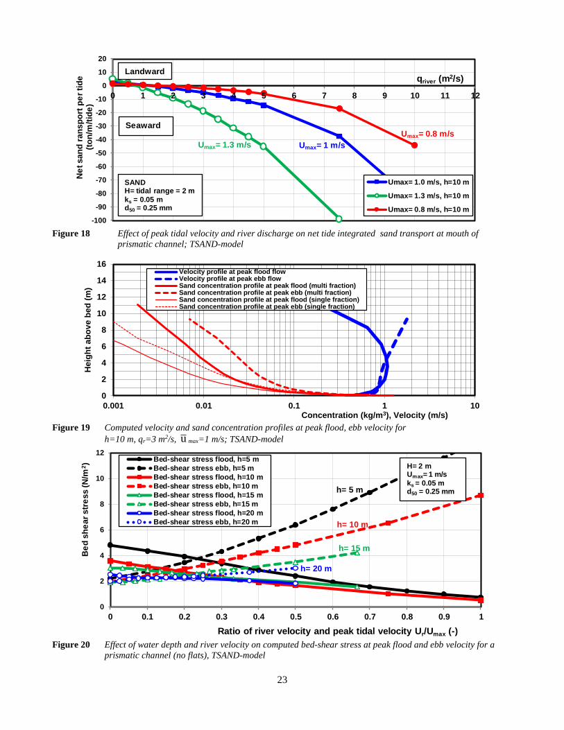
23

Figure 18 Effect of peak tidal velocity and river discharge on net tide integrated sand transport at mouth of

prismatic channel; TSAND-model

Figure 19 Computed velocity and sand concentration profiles at peak flood, ebb velocity for

h=10 m, qr=3 m2/s, max=1 m/s; TSAND-model

Figure 20 Effect of water depth and river velocity on computed bed-shear stress at peak flood and ebb velocity for a

prismatic channel (no flats), TSAND-model

-100

-90

-80

-70

-60

-50

-40

-30

-20

-10

0

10

20

0 1 2 3 4 5 6 7 8 9 10 11 12

Ne

t san

d r

an

sp

ort

pe

r ti

de

(t

on

/m/t

ide

)

qriver (m2/s)

Umax= 1.0 m/s, h=10 m

Umax= 1.3 m/s, h=10 m

Umax= 0.8 m/s, h=10 m

Landward

Seaward

SAND H= tidal range = 2 m

ks = 0.05 m d50 = 0.25 mm

Umax= 1 m/sUmax= 1.3 m/s

Umax= 0.8 m/s

0

2

4

6

8

10

12

14

16

0.001 0.01 0.1 1 10

Heig

ht

ab

ov

e b

ed

(m

)

Concentration (kg/m3), Velocity (m/s)

Velocity profile at peak flood flowVelocity profile at peak ebb flowSand concentration profile at peak flood (multi fraction)Sand concentration profile at peak ebb (multi fraction)Sand concentration profile at peak flood (single fraction)Sand concentration profile at peak ebb (single fraction)

u

0

2

4

6

8

10

12

0 0.1 0.2 0.3 0.4 0.5 0.6 0.7 0.8 0.9 1

Be

d s

he

ar

str

es

s (N

/m2)

Ratio of river velocity and peak tidal velocity Ur/Umax (-)

Bed-shear stress flood, h=5 m

Bed-shear stress ebb, h=5 m







H= 2 m Umax= 1 m/s

ks = 0.05 m d50 = 0.25 mmh= 5 m

h= 10 m

h= 15 m

h= 20 m

24

4.3 Discussion

The consequences of the results of Figures 17 to 20 can be best explained by an example of a prismatic tidal channel with a

sandy bed such as the Rotterdam Waterway. For this purpose we consider two fixed locations: upstream river section (no tide)

and downstream tidal mouth region, both with an equal water depth of 5 m. The upstream sand transport for a depth of 5 m

and a river discharge of 4.5 m2/s (river velocity of 0.9 m/s; Rhine river) is about 12 ton/m/tide (export to the sea, Figure 17).

The sand export in the tidal mouth region at a depth of 5 m and at the same river discharge of 4.5 m2/s is about 100 ton/m/tide

(Figure 17). Thus, the net transport rate in the tidal channel section (with depth of 5 m) increases considerably (from 12 to

100 ton/m/tide) due to the presence of tide-induced and salinity-induced flows resulting in erosion. At a water depth of about

10 m in the mouth region, the net transport rate is about equal to 12 ton/m/tide (export) being the transport rate of the upstream

river section (with depth of 5 m). Thus, a water depth of 10 m can be seen as the ‘equilibrium’ water depth of the tidal channel

in the mouth region. This example shows that the depths of the tide-influenced sections need to be much larger than the depths

of the more inland sections to obtain quasi-equilibrium conditions with a constant transport rate along the channel. The water

depths along the tidal section of the river will gradually (exponentially) increase in seaward direction to the ‘equilibrium’

water depth of 10 m at the mouth.

For water depths smaller than the ‘equilibrium’ depth, erosion will occur until the depth is equal to the equilibrium depth.

For water depths larger (due to dredging) than the ‘equilibrium’ depth, deposition will dominate in the tidal section (regime

shift from erosion to deposition). If the channel banks are erodible (no dikes or groins), both the width and depth of the channel

will adjust to form a converging tidal channel.

Around 1900 the water depth of the Rotterdam Waterway was about 8 to 10 m, which could be maintained without dredging

except for the mouth region with sand deposition in the jetty opening (Staatscommissie, 1920). Thus, a water depth of 8 to 10

m can be seen as the equilibrium depth of the Rotterdam Waterway in a regime with export of sand for discharges of about 3

m2/s (see Figure 17).

For navigational purposes it is often required to have a relatively deep tidal channel with constant water depth. Based on

Figure 17 (sandy bed), the net transport rate will decrease for larger depths than the ‘equilibrium’ depth resulting in channel

deposition. For example, if h=15 m, qr= 4.5 m2/s and max= 1 m/s, it follows that qs,net 2 ton/m/tide (export). This latter

value is much smaller (factor 6) than the net transport of 12 ton/m/tide (export) in the upstream river-dominated section where

the depth is 5 m. The difference of 10 ton/m/tide will be deposited in the deeper tidal channel (15 m). Using a channel width

of 500 m, 730 tides per year and a bulk density of 1.5 ton/m3, the deposition volume (mainly river sediments) will be about

10x500x730/1.5 2.5 million m3/year.

This example shows that channel deepening in a prismatic channel beyond the ‘equilibrium’ depth will always result in

significant deposition and associated dredging in the tidal section. Further deepening of an already deep channel from 15 m

to 20 m only leads to a marginal increase of the deposition volume as the net tide-integrated transport rate (export) at the

mouth decreases from about 2 to 1 ton/m/tide, which is equivalent with an additional deposition volume of about 0.25 million

m3/year for a channel of 500 m wide.

5. Conclusions

In this paper we have identified and discussed the basic processes influencing the sand transport processes in tidal channels.

We presented a simplified model for tide- and density-driven currents and resulting sand transport rates and verified these

with field data of the Rotterdam Waterway. The advantage of the simplified TSAND-model is the rapid assessment of the net

tide-integrated sand transport (import or export) at locations in the mouth region of a tidal channel for a range of hydrodynamic

and sediment conditions including storm events (sensitivity studies). The simplified TSAND-model is a powerful tool to

determine the most influencial processes and parameters so that the number of detailed 2DH or 3D model runs can be reduced.

The most important findings of the present study are:

1. Channel deepening of a prismatic channel (Rotterdam Waterway) from 10 to 20 m leads to less tidal damping;

slightly larger tidal ranges (<10%) and slightly larger peak tidal velocities (<10%) in mouth region (< 25 km).

2. Channel deepening from a small depth of about 5 m to a larger depth of 10 m in strongly converging channels

may lead to a regime shift from tidal damping to tidal amplification with a much larger tidal range; the peak

tidal velocities in the mouth region (< 25 km) remain fairly constant.

3. The tidal velocity asymmetry values in the mouth of a tidal channel are in the range of 1 and 1.2 (flood

dominance) depending on the ratio of the tidal amplitude and the water depth for natural tidal channels with no

or minor intertidal flats.

4. The net tide-integrated sand transport of sandy tidal channels can be determined with sufficient accuracy by the

simplified TSAND-model coupled to 1D, 2DH or 3D hydrodynamic models.

5. Based on the results of the simplified sand transport model, an equilibrium depth can be defined for prismatic

and/or weakly converging tidal channels; the equilibrium depth is the depth at which the net tide-integrated

sediment transport is equal to the sediment transport in the steady upstream river flow.

u

25

6. The equilibrium depth of tidal channels is much larger (factor of 2) than the upstream river depth for sandy

channels. Deposition occurs for channel depths larger than the equilibrium depth.

7. The further deepening (10% to 20%) of an already deep tidal channel (> 15 m; Rotterdam Waterway) has a

marginal effect on the tide-integrated transport rates, the deposition rates and the dredging volumes (no tipping

point effects).

8. The change from import to export of sediment at the mouth of a tidal channel (Rotterdam Waterway) occurs

for fresh water (river) discharges larger than 1 to 3 m2/s in the case of a sandy bed.

Acknowledgements

Pieter Koen Tonnon and Bas van Maren of Deltares (The Netherlands) are gratefully acknowledged for providing 3D-model

results for various cases/sites. Both reviewers are acknowledged for their detailed, critical comments to improve the quality

of the paper. The studies on the Rotterdam Waterway were done by both co-authors when they were employed by Arcadis

Consultancy in The Netherlands. Arcadis is gratefully acknowledged for the permsission to publish these results.

References

Amin, M., 1983. On perturbations of harmonic constants in the Thames estuary. Geophysical Journal of the Royal

Astronomical Society, 73(3), 587–603.

Arcadis, 2015. Deepening of Rotterdam Waterway and Botlek; morphology study. Report C03041.002053.0100 (in Dutch)

BAW, Bundes Anstalt für Wasserbau, 2006. Gutachten zur ausbaubedingten Aenderung der morphodynamischen

Prozesse (in German), Report H1c, www.fahrrinnenausbau.de

Brenou, I. and Le Hir, P. 1999. Modelling the turbidity maximum in the Seine estaury (France). Estuarine, Coastal and Shelf

Science 49, 525-544

Burchard H. and Baumert H., 1998. The formation of estuarine turbidity maxima due to density effects in the salt wedge.

A hydrodynamic process study. Journal of Physical Oceanography, 28, 2, 309-320.

Chatwin, P.C., 1976. Some remarks on the maintenance of the salinity distribution in estuaries. Estuarine and Coastal Marine

Science, Vol. 4, 555-566

Chernetsky, A., Schuttelaars, H. and Talke, S., 2010. The effect of tidal asymmetry and temporal settling lag on sediment

trapping in tidal estuaries. Ocean Dynamics. 60, 1219–1241.

Deltares/Delft Hydraulics 1980. Computation of siltation in dredged trenches. Report R1267 V, Delft, The Netherlands

Deltares 2011. Tidal phenomena in the Scheldt estuary, part 2. Report 1204410, Delft, The Netherlands De Jonge, V.N., Schuttelaars H.M., Van Beusekom J.E.E., Talke S.A., De Swart,H.E., 2014. The influence of channel deepening on estuarine turbidity levels and dynamics, as exemplified by the Ems estuary. Estuarine Coastal Shelf Science. doi:10.1016/j.ecss.2013.12.030 DiLorenzo J.L., Huang P., Thatcher M.L. and Najarian T.O.. 1993. Dredging impacts on Delaware Estuary tides.

Presented at the 3rd International Conference on Estuarine and Coastal Modeling III, 86-104, Oak Brook, Illinois, USA

Dronkers, J.J., 1964. Tidal computations in rivers and coastal waters. p. 518. North-Holland, New York

Familkhalili, R. and Talke, S.A. 2016. The effect of channel deepening on tides and storm surge: A case study of

Wilmington, NC. Geophysical Research Letters 43,9138-9147

Friedrichs, C.T. 2010. Barotropic tides in channelized estuaries. Contemporay Issues in Estuarine Physics, 27-61, Cambridge

University Press

Friedrichs, C.T. and Aubrey, D.G., 1988. Non-linear tidal distortion in shallow well-mixed estuaries; a synthesis. Estuarine,

Coastal and Shelf Science, 27, 521-545

Hansen, D.V. and Rattray, M., 1965. Gravitational circulation in straits and estuaries. Journal Marine Res. 23, 104–122.

Herrling, G. and Niemeyer, H.D., 2008. Comparison of the hydrodynamic regime of 1937 and 2005 in the Ems estuary by

applying mathematical modeling. Harbasins report, 30 p.

Herrling, G., Elsebach, J. and Ritzmann, 2014. Evaluation of changes in the tidal regime of the Ems-Dollard and lower

Weser estuaries by mathematical modelling. Die Kuste, 81, 353-368

Hollebrandse, F.A.P., 2005. Temporal development of the tidal range in the southern North Sea. MSc. Thesis, Civil

Engineering, Delft University of Technology, Delft, The Netherlands

Kuijper, K. and Van Rijn, L.C., 2011. Analytical and numerical analysis of tides and salinities in estuaries;

Part II: salinity distributions in prismatic and convergent tidal channels. Ocean Dynamics, Vol. 61, 1743-1765

Lesser, G., Roelvink, J.A., Van Kester, J.A.T.M. and Stelling, G.S., 2004. Development and validation of a three-

dimensional morphological model. Journal of Coastal Engineering Vol. 51, p 883-915.

Lorentz, H.A., 1922. Including resistance in tidal flow equations (in Dutch). De Ingenieur, p. 695, The Netherlands.

Lorentz, H.A., 1926. Report Commission Zuiderzee 1918-1926 (in Dutch). Den Haag, The Netherlands.

Nikuradse, J., 1933. Strömungsgesetze in rauhen Rohren. Forschungsarbeiten aus dem Gebiete des Ingenieurwesens, Ver.

Deut. Ing. Forschungsheft 361, Berlin, Germany

Prandle, D., 1985. On salinity regimes and the vertical structure of residual flows in narrow estuaries. Estuarine, Coastal and

Shelf Science, Vol. 20, 615-635

http://dx.doi.org/10.1016/j.ecss.2013.12.030

http://dx.doi.org/10.1016/j.ecss.2013.12.030

26

Prandle, D., 2004. Saline intrusion in partially mixed estuaries. Estuarine, Coastal and Shelf Science, Vol. 59, 385-397 Prandle, D., 2009. Esturies. Dynamics, Mixing, Sedimentation and Morphology. Cambridge University Press.

Rijkswaterstaat 2017. Internet tidal database (getij.rws.nl)

Talke S.A., De Swart H.E. and Schuttelaars H.M., 2009. Feedback between residual circulations and sediment

distribution in highly turbid estuaries: an analytical model. Continental Shelf Research 29, 119–135.

doi:10.1016/j.csr.2007.09.002

Van de Kreeke, J. and Haring, J., 1979. Equilibrium flow areas in Rhine-Meuse Delta. Cosatal Engineering, 3, 97-111

Van Maren, D.S., Van Kessel, T., Cronin, K. and Sittoni, L., 2015a. The impact of channel deepening on estuarine

sediment concentration. Continental Shelf Research, Vol. 95, 1-14

Van Maren, D.S., Winterwerp, J.C. and Vroom, J., 2015b. Fine sediment transport into the hyper-turbid lower Ems

River: the role of channel deepening and sediment-induced drag reduction. Ocean Dynamics, DOI 10, 1007/s/10236-015-

0821-2

Van Rijn, L.C., 1984a. Sediment Transport, Part I: Bed Load Transport. Journal of Hydraulic Engineering, ASCE, Vol. 110,

No. 10.

Van Rijn, L.C., 1984b. Sediment Transport, Part II: Suspended Load Transport. Journal of Hydraulic Engineering, ASCE, Vol.

110, No. 11.

Van Rijn, L.C., 1984c. Sediment Transport, Part III: Bed Forms and Alluvial Roughness. Journal of Hydraulic Engineering,

ASCE, Vol. 110, No. 12.

Van Rijn, L.C., 1987. Mathematical modelling of morphological processes in the case of suspended sediment transport.

Doctoral Thesis. Department of Civil Engineering, Delft University of Technology, Delft, The Netherlands

Van Rijn, L.C., 1993. Principles of sediment transport in rivers, estuaries and coastal seas. www.aquapublications.nl

Van Rijn, L.C., 2007. Unified view of sediment transport by currents and waves, I, II, III. ASCE, Journal of Hydraulic

Engineering, Vol. 133, No. 6, 649-667, 668-689, No. 7, 761-775

Van Rijn, L.C., 2011a. Principles of fluid flow and surface waves in rivers, estuaries and coastal seas.

www.aquapublications.nl

Van Rijn, L.C., 2011b. Analytical and numerical analysis of tides and salinities in estuaries;

Part I: tidal wave propagation in convergent tidal channels. Ocean Dynamics, Vol. 61, 1719-1741

Van Rijn 2015. Principles of sedimentation and erosion engineering in rivers, estuaries and coastal seas.

www.aquapublications.nl

Voogt, L., Van Rijn, L.C. and Van Den Berg, J.H., 1991. Sediment transport of fine sands at high velocities. Journal of

Hydraulic Engineering, ASCE, Vol. 117, No. 7.

Winterwerp, J.C., 2001. Stratification effects by cohesive and non cohesive sediment. Journal of Geophysical Research, Vol.

106, No C10, 22,559-22,574

Winterwerp, J.C., 2011. Fine sediment transport by tidal asymmetry in the high-concentrated Ems river: indications for a

regime shift in response to channel deepening. Ocean Dynamics 61, 203-215

Winterwerp, J.C. and Wang, Z.B., 2013. Man-induced regime shifts in small estuaries-I: theory. Ocean Dynamics,

DOI10.1007/s10236-013-0662-9

http://www.aquapublications.nl/






effect of channel deepening on tidal flow and …

Documents