.

Email: klaus.ehrenfried@dlr.de

Effects of Wind-Tunnel Noiseon Array Measurements in Closed Test Sections

K. Ehrenfried1, L. Koop1, A. Henning2 and K. Kaepernick2

1Institute of Aerodynamics and Flow TechnologyGerman Aerospace Center (DLR), Gottingen

2Institut fur Luft und RaumfahrtTechnical University of Berlin

1

Overview

• Motivation

• Experimental setup

• Source maps

• Effects of background noise

• Wavenumber spectrum

• Algorithm to remove noise effect in source maps

• Improved results

Background noise 2

Motivation

• Economic efficiency in aerodynamic and aeroacoustic testing

– Aerodynamic and aeroacoustic tests in parallel

• Acoustically optimized wind tunnels

– Open jet configuration in anechoic chamber

– Surfaces line with absorbing material

– Little background noise

• Aerodynamic measurements

– Closed test sections

– Well defined boundary conditions

– Ideal for comparison with numerical results

=⇒ Aeroacoustic experiments in closed test sections

Background noise 3

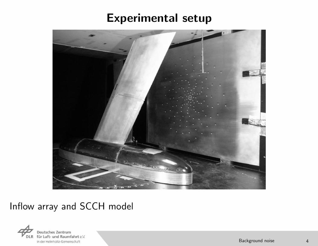
Experimental setup

Inflow array and SCCH model

Background noise 4

Experimental parameters

• Wind tunnel

– 2.0m × 1.4m test section, hard side walls

– 30 m/s flow velocity

• Array

– 144 microphones on 9 spiral arms, 1 m diameter of microphone field

– 25 mm thick array body

– Electret microphones (RTI)

– 120 kHz sampling frequency, 30 sec measurement time

• Wing model

– Swept-wing constant-chord half-model (SCCH model)

– 1.2m span, 0.4 m chord

– Slat deployed, flap retracted, 7 degree angle of attack

Background noise 5

Point of view

Inflow array and SCCH model (upside down)

Background noise 6

Array processing

• Delay-and-sum beamforming in frequency domain

• 4096 samples window length (rectangle), ∆f = 29.3 Hz

• Diagonal removal

• 10 mm source map resolution

• Observation plane turned with SCCH model

• Array maps using local coordinates

• Assumption of homogeneous flow (U = 30 m/s)

• Model-frequency scaling ≈ 1:6

Background noise 7

Beamforming results

f = 7500 Hz (narrow band)

Background noise 8

Beamforming results

f = 15000 Hz (narrow band)

Background noise 9

Beamforming results

f = 30000 Hz (narrow band)

Background noise 10

Beamforming results

f = 30000 Hz (1/3 octave)

Background noise 11

Beamforming results

f = 3750 Hz (narrow band)

Background noise 12

Beamforming results

f = 2900.4 Hz (narrow band)

Background noise 13

Opposite side wall lined with absorbing layer

30 mm thick foam layer

Background noise 14

Effect of absorbing layer

Untreated side wall With foam layer

f = 2900.4 Hz (narrow band)

Background noise 15

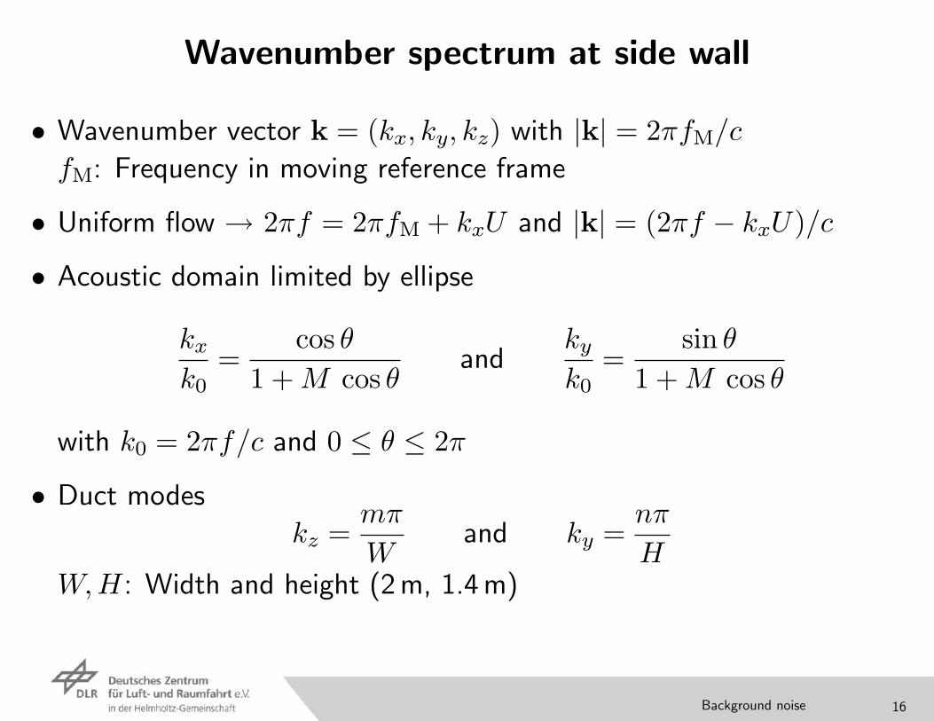
Wavenumber spectrum at side wall

• Wavenumber vector k = (kx, ky, kz) with |k| = 2πfM/c

fM: Frequency in moving reference frame

• Uniform flow → 2πf = 2πfM + kxU and |k| = (2πf − kxU)/c

• Acoustic domain limited by ellipse

kx

k0=

cos θ

1 + M cos θand

ky

k0=

sin θ

1 + M cos θ

with k0 = 2πf/c and 0 ≤ θ ≤ 2π

• Duct modes

kz =mπ

Wand ky =

nπ

HW,H: Width and height (2m, 1.4m)

Background noise 16

Acoustic domain

U = 30 m/s (M ≈ 0.088), 720 duct modes “cut on” (f = 2900 Hz)

Background noise 17

Estimation of the wavenumber spectrum

• Beamforming with an infinite focus distance

• Steering vector

sj = exp [−i(kxxj + kyyj)]

(xj, yj): Position of j-th microphone

• Map in wavenumber space

• Normalization with k0 = 2πf/c

• Summation over 1/3-octave of values for fix (kx/k0, ky/k0)

Background noise 18

Maps in wavenumber space

Untreated side wall With foam layer

f = 3000 Hz (1/3-octave)

Background noise 19

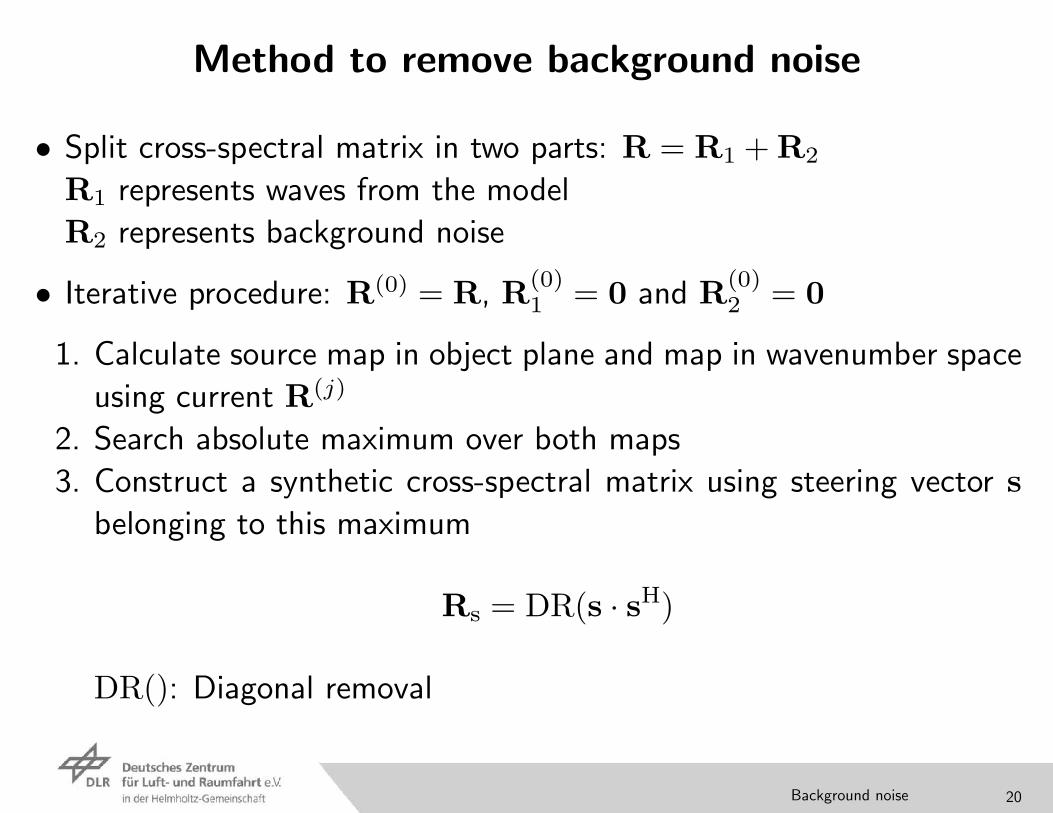
Method to remove background noise

• Split cross-spectral matrix in two parts: R = R1 + R2

R1 represents waves from the model

R2 represents background noise

• Iterative procedure: R(0) = R, R(0)1 = 0 and R(0)

2 = 0

1. Calculate source map in object plane and map in wavenumber space

using current R(j)

2. Search absolute maximum over both maps

3. Construct a synthetic cross-spectral matrix using steering vector sbelonging to this maximum

Rs = DR(s · sH)

DR(): Diagonal removal

Background noise 20

Method to remove background noise

4. Normalize synthetic cross-spectral matrix

Rs = Rs

(sH R(j) ssH Rs s

)

5. Set R(j+1) = R(j) − Rs

6. If absolute maximum belongs to source map in object plane then

{ R(j+1)1 = R(j)

1 + Rs } else { R(j+1)2 = R(j)

2 + Rs }

• Iteration can be stopped when maximum is below predetermined

threshold (here: 200 iterations)

• Remaining R(j) is added to R(j)1 and then R(j)

1 is taken as new

cross-spectral matrix to replace the initial R

Background noise 21

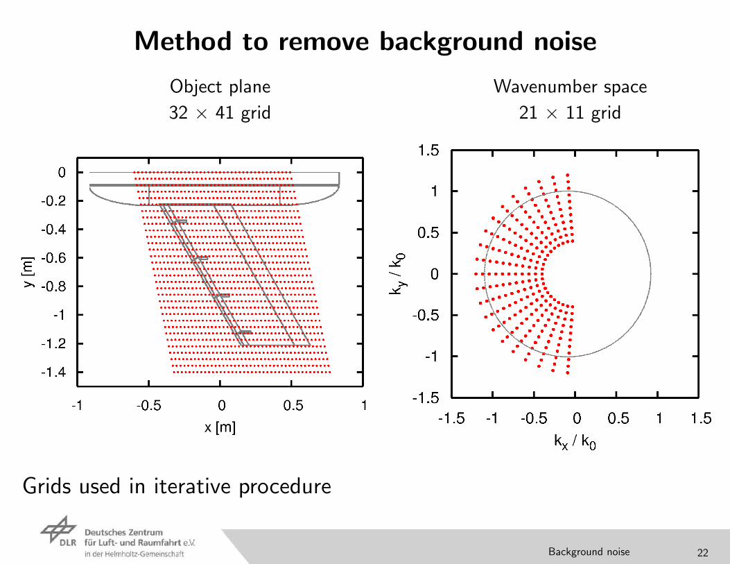
Method to remove background noise

Object plane

32 × 41 grid

Wavenumber space

21 × 11 grid

Grids used in iterative procedure

Background noise 22

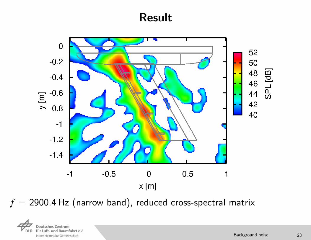
Result

f = 2900.4 Hz (narrow band), reduced cross-spectral matrix

Background noise 23

Comparison

Raw cross-spectral matrix Reduced cross-spectral matrix

f = 2900.4 Hz (narrow band)

Background noise 24

Concluding remarks

• Strong background noise present in wind tunnels with closed test

sections

• Upstream propagating waves

• Waves cause artifacts in source maps

• Iterative method to remove artifacts caused by plane waves

• Further testing in other wind tunnels required

Background noise 25