EE599-020Audio Signals and Systems

Psychoacoustics (Masking)

Kevin D. DonohueElectrical and Computer Engineering

University of Kentucky

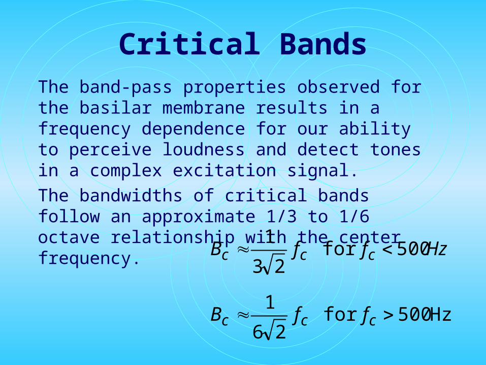
Critical BandsThe band-pass properties observed for the basilar membrane results in a frequency dependence for our ability to perceive loudness and detect tones in a complex excitation signal.

The bandwidths of critical bands follow an approximate 1/3 to 1/6 octave relationship with the center frequency.

Hz 500for 26

1

500for 23

1

ccc

ccc

ffB

HzffB

Loudness and Critical Band

Tones separated by distances greater than the critical band are perceived louder than the same tones within a critical band.

Broadband noises spanning several critical bands are perceived louder than broadband noise of the same power within one critical band.

Example Broadband

A function was created to generate white Gaussian noise with unit power in a designated frequency band and specific sampling rate. A series of band pass filters and scalings were applied to keep the power in the noise constant with frequency bands reducing on a center frequency around 2120 Hz.

500 1000 1500 2000 2500 3000 3500 4000

0

0.5

1

1.5

2

2.5

x 10-3

Hertz

PD

S

Approximate Critical Band

Example Broadband Signal Spectra

Number of critical bands in each sound

14.7

8.1

2.2

1.0

0.5

0.2

Sound Sequence: Starting with the largest band

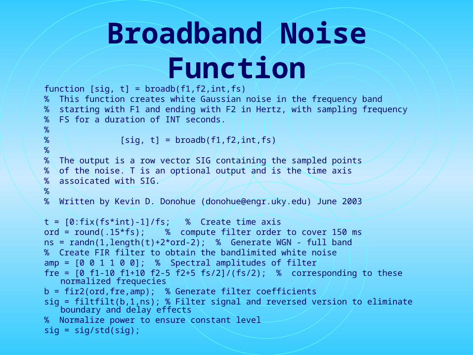
Broadband Noise Functionfunction [sig, t] = broadb(f1,f2,int,fs)% This function creates white Gaussian noise in the frequency band% starting with F1 and ending with F2 in Hertz, with sampling frequency % FS for a duration of INT seconds.%% [sig, t] = broadb(f1,f2,int,fs)%% The output is a row vector SIG containing the sampled points% of the noise. T is an optional output and is the time axis% assoicated with SIG. %% Written by Kevin D. Donohue (donohue@engr.uky.edu) June 2003

t = [0:fix(fs*int)-1]/fs; % Create time axisord = round(.15*fs); % compute filter order to cover 150 msns = randn(1,length(t)+2*ord-2); % Generate WGN - full band% Create FIR filter to obtain the bandlimited white noiseamp = [0 0 1 1 0 0]; % Spectral amplitudes of filterfre = [0 f1-10 f1+10 f2-5 f2+5 fs/2]/(fs/2); % corresponding to these normalized frequeciesb = fir2(ord,fre,amp); % Generate filter coefficients sig = filtfilt(b,1,ns); % Filter signal and reversed version to eliminate boundary and delay effects% Normalize power to ensure constant levelsig = sig/std(sig);

Broadband Noise Script• % This script generates 6 example noise signals, with• % sucessively smaller bandwidths. The last 2 are within• % the critical band.• % The average spectrum (PSD) for each is plotted and the• % signals are concatenated together as save as a wave file.• % You need the functions BARKCOUNT and BROADB• % to run this script.• %• % Written by Kevin D. Donohue (donohue@engr.uky.edu)• % February 2004

• fs = 11025; % Sampling Frequency• dur = 2; % Sound duration in seconds• % Vectors describing the sucessive bandlimit on the sounds• f1 = [270, 1000, 1800, 2000, 2050, 2100]; % lower limit• % corresponding upper bandlimit• f2 = [4000, 3500, 2500, 2320, 2220, 2150];• % colors for the PSD plots• col = ['g', 'r', 'b', 'k', 'c', 'b'];• % Loop to create each sound and concatenate into one• % vector• fsig = []; % Initialize vector to concatenate sounds

for k=1:length(f1);

• % Generate noise

• no(k,:) = broadb(f1(k), f2(k), dur, fs);

• fsig = [fsig, no(k,:)]; % Concatenate

• % Count the bark (Critical Bands)

• cb(k) = barkcount(f1(k),f2(k));

• % Compute PSD of noise

• [p, fax] = psd(no(k,:),1024, fs, hamming(512));

• figure(1);

• % Plot PSD

• lh = plot(fax,abs(p)/(length(no(k,:))),col(k))

• set(lh,'LineWidth',2) % Make line thicker

hold on

• end

• hold off

• % Label figure

• xlabel('Hertz')

• ylabel('PDS')

• % Write sound to wavefile

• wavwrite(fsig/(max(abs(fsig)+eps)), fs, 'wgncritband.wav')

Example Discussion

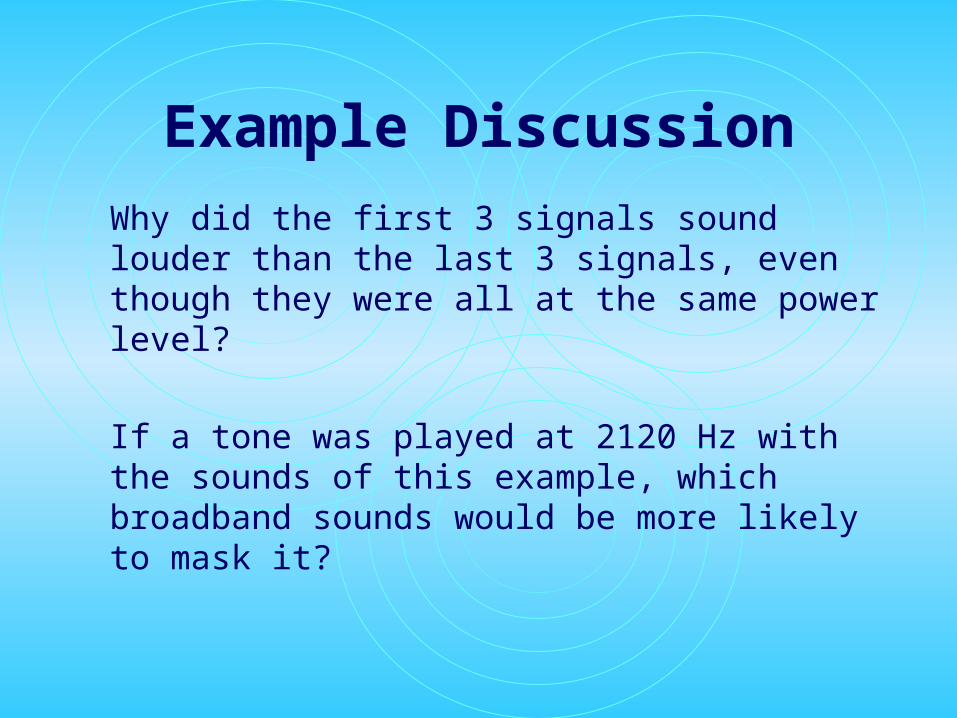
Why did the first 3 signals sound louder than the last 3 signals, even though they were all at the same power level?

If a tone was played at 2120 Hz with the sounds of this example, which broadband sounds would be more likely to mask it?

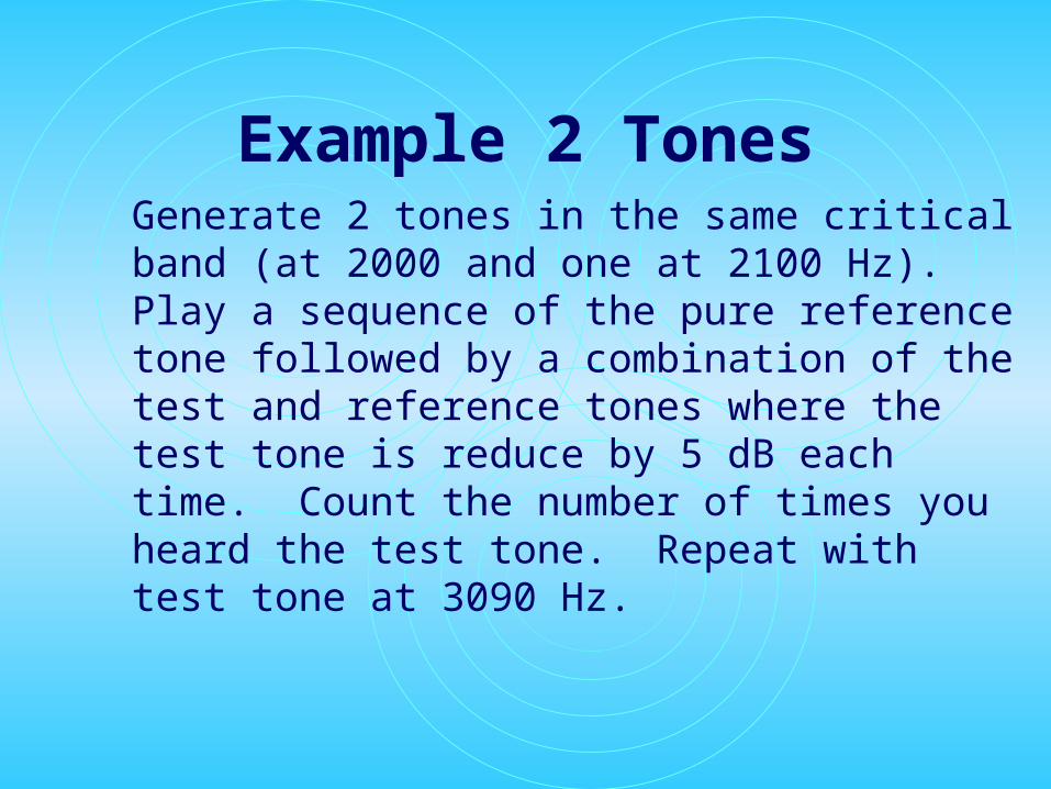
Example 2 TonesGenerate 2 tones in the same critical band (at 2000 and one at 2100 Hz). Play a sequence of the pure reference tone followed by a combination of the test and reference tones where the test tone is reduce by 5 dB each time. Count the number of times you heard the test tone. Repeat with test tone at 3090 Hz.

Example 2 Tones Spectrogram

Seconds

Her

tz

Masking Illustration: 2000 masking 2100

0 5 10 15 20 251500

2000

2500

3000

3500

20

25

30

35

40

45

dB 2000 Hz and2100 Hz pair

Example 2 Tones Spectrogram

Seconds

Her

tz

0 5 10 15 20 251500

2000

2500

3000

3500

20

25

30

35

40

452000 Hz and3090 Hz pair

2-Tone Function• function [v, t] = tonec(f,int,fs)• % This function will create a series of samples at sampling rate• % FS for a duration of INT seconds at frequencies in the frist column• % of vector F in Hertz. The second column of F will be the weight for • % each tone. If a second column is not given then an equal scaling of • % of will be given to each tone.• %• % [v, t] = tonec(f,int,fs)• %• % The output is a row vector V containing the sampled points• % T is an optional output and is the time axis assoicated with V.• %• % Written by Kevin D. Donohue (donohue@engr.uky.edu) 6/2003• [r, c] = size(f); % Check dimension of f• % Ensure frequency values are in different rows• if c > 2 % if not transpose• f = f';• [r, c] = size(f);• end• % Check to see if coefficients for frequenies are provided• if c == 1 % If not set them = to one• f(:,2) = ones(length(f),1);• end• t = [0:fix(fs*int)-1]/fs; % Create time axis• v = zeros(size(t)); % initialize vector to accumulate multiple tones• for k=1:r• v = v + f(k,2)*sin(2*pi*t*f(k,1)); % Create sampled tone signal• end

2-Tone Script• % This script generates tone pair signals, with successively• % smaller amplitudes on a test to illustrate masking• % The signal pair are generate individually and concatenate• % together with silence and reference tones stuffed in between• % and saved as a wave file.• % This script needs the TONEC function to run.• %• % Written by Kevin D. Donohue (donohue@engr.uky.edu) June 2003• fs = 11025; % Sampling Frequency• dur = 1; % Tone duration• reffre = 2000; % Reference tone• tfre = 2100; % Test tone with decreasing volume• % Vector with sequence of relative volume levels• tamp = 10.^([0 -5 -10 -15 -20 -25 -30 -35 -40 -45]/20);• reftone = tonec([reffre 1], dur, fs); % Generate Reference tone signal• outsig = []; % Initalize output matrix for concatenation • scil = zeros(1,round(fs*dur/2)); % Create silence interval• % Loop to build complex tone, concatenation with reference and rest of• % sequence• for k=1:length(tamp)• ttone = tonec([reffre 1; tfre tamp(k)], dur, fs);• outsig = [outsig scil reftone scil std(reftone)*ttone/std(ttone)];• end

• (Continued on next slide …)

2-Tone Script - Continued• % Write test signal• wavwrite(outsig/(max(abs(outsig)+eps)), fs, 'testttsig2.wav')• % Create and plot spectrogram• [B,F,T] = SPECGRAM(outsig,4*512,fs,hamming(4*256),4*128);• imagesc(T,F,20*log10(abs(B)+10))• axis('xy')• axis([T(1) T(end) 1500 3500])• xlabel('Seconds')• ylabel('Hertz')• title(['Masking Illustration: ' num2str(reffre) ' masking ' num2str(tfre)])• colorbar

2-Tone DiscussionHow many times did you hear the test tone for the 2000 and 2100 Hz pair? How many times did you hear the test tone for the 2000 and 3090 Hz pair?Estimate the masking threshold for tones separated by 100 Hz near 2000 Hz.Estimate the masking threshold for tones separated by 1090 Hz near 2000 Hz.Why is there a difference?

Is it possible to eliminate the beat frequencies for closely place tones?

Gammatone Filters

The Gammatone filter:Is physically realizable (causal)

Provides a good fit to the impulse response of the auditory nerve fibers (Carney and Yin 1988, J. Neurophys. 60, 1653-1677).

Gammatone Filters

The Gammatone filter impulse response:

0for 0

0for )2cos()2exp()(

)1(

t

ttfbttbth c

where = 4, fc is the center frequency, and b is set to match the bandwidth of the critical band.