ee365: markov chains - stanford university markov chains ... cgis inventory level at time t ... i we...
TRANSCRIPT

EE365: Markov Chains
Markov chains
Transition Matrices
Distribution Propagation
Other Models
1

Markov chains
2

Markov chains
I a model for dynamical systems with possibly uncertain transitions
I very widely used, in many application areas
I one of a handful of core effective mathematical and computational tools
I often used to model systems that are not random; e.g., language
3

Stochastic dynamical system representation
xt+1 = f(xt, wt) t = 0, 1, . . .
I x0, w0, w1, . . . are independent random variables
I state transitions are nondeterministic, uncertain
I combine system xt+1 = f(xt, ut, wt) with policy ut = µt(xt)
4

Example: Inventory model with ordering policy
xt+1 = [xt − dt + ut][0,C] ut = µ(xt)
I xt ∈ X = 0, . . . , C is inventory level at time t
I C > 0 is capacity
I dt ∈ 0, 1, . . . is demand that arrives just after time t
I ut ∈ 0, 1, . . . is new stock added to inventory
I µ : X → 0, 1, . . . , C is ordering policy
I [z][0,C] = min(max(z, 0), C) (z clipped to interval [0, C])
I assumption: d0, d1, . . . are independent
5

Example: Inventory model with ordering policy
xt+1 = [xt − dt + ut][0,C] ut = µ(xt)
I capacity C = 6
I demand distribution pi = Prob(dt = i)
p =[0.7 0.2 0.1
]I policy: refill if xt ≤ 1
µ(x) =
C − x if x ≤ 10 otherwise
I start with full inventory x0 = C
6
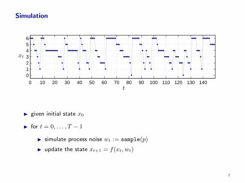
Simulation
0 10 20 30 40 50 60 70 80 90 100 110 120 130 140
0123456
xt
t
I given initial state x0
I for t = 0, . . . , T − 1
I simulate process noise wt := sample(p)
I update the state xt+1 = f(xt, wt)
7

Simulation
I called a particle simulation
I gives a sample of the joint distribution of (x0, . . . , xT )
I useful
I to approximately evaluate probabilities and expectations via Monte Carlosimulation
I to get a feel for what trajectories look like (e.g., for model validation)
8

Graph representation
0 1 2 3 4 5 6
p1p1p1p1p1
p0p0p0p0p0
p2p2p2p2p2
p0
p1
p2 p0
p1
p2
I called the transition graph
I each vertex (or node) corresponds to a state
I edge i→ j is labeled with transition probability Prob(xt+1 = j | xt = i)
9

The tree
1
2
31
0.5
0.4
0.5
0.6
2
2
2
2
0.5
3
0.5
0.5
3
1
0.4
3
0.6
0.5
0.5
3
1
2
1
0.4
3
1
0.4
3
0.6
0.6
0.5
I each vertex of the tree corresponds to a path
I e.g., Prob(x3 = 1 |x0 = 2) = 0.5× 0.5× 0.4 + 0.5× 0.6× 0.4
10

The birth-death chain
1 2 3 4 5 6
0.1 0.1 0.1 0.1
0.6 0.6 0.6 0.6 0.6
0.3 0.3 0.3 0.3 0.3
0.4 0.7
self-loops can be omitted, since they can be figured out from the outgoing proba-bilities
11
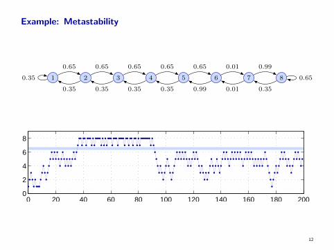
Example: Metastability
1 2 3 4 5 6 7 80.35 0.65
0.65 0.65 0.65 0.65 0.65 0.01 0.99
0.35 0.35 0.35 0.35 0.99 0.01 0.35
0 20 40 60 80 100 120 140 160 180 2000
2
4
6
8
12
Transition Matrices
13

Transition matrix representation
we define the transition matrix P ∈ Rn×n
Pij = Prob(xt+1 = j | xt = i)
I P1 = 1 and P ≥ 0 elementwise
I a matrix with these two properties is called a stochastic matrix
I if P and Q are stochastic, then so is PQ
14

Transition matrix representation
0 1 2 3 4 5 6
p1p1p1p1p1
p0p0p0p0p0
p2p2p2p2p2
p0
p1
p2 p0
p1
p2
transition matrix
P =
0 0 0 0 0.1 0.2 0.70 0 0 0 0.1 0.2 0.7
0.1 0.2 0.7 0 0 0 00 0.1 0.2 0.7 0 0 00 0 0.1 0.2 0.7 0 00 0 0 0.1 0.2 0.7 00 0 0 0 0.1 0.2 0.7
15

Particle simulation given the transition matrix
Given
I the distribution of initial states d ∈ R1×n
I the transition matrix P ∈ Rn×n, with rows p1, . . . , pn
Algorithm:
I choose initial state x0 := sample(d)
I for t = 0, . . . , T − 1
I find the distribution of the next state dnext := pxt
I sample the next state xt+1 := sample(dnext)
16

Definition of a Markov chain
sequence of random variables xt : Ω → X is a Markov chain if, for all s0, s1, . . .and all t,
Prob(xt+1 = st+1|xt = st, . . . , x0 = s0) = Prob(xt+1 = st+1|xt = st)
I called the Markov property
I means that the system is memoryless
I xt is called the state at time t; X is called the state space
I if you know current state, then knowing past states doesn’t give additionalknowledge about next state (or any future state)
17

The joint distribution
the joint distribution of x0, x1, . . . , xt factorizes according to
Prob(x0 = a, x1 = b, x2 = c, . . . , xt = q
)= daPabPbc · · ·Ppq
because the chain rule gives
Prob(xt = st, xt−1 = st−1, . . . , x0 = s0)
= Prob(xt = st |xt−1 = st−1, . . . , x0 = s0)Prob(xt−1 = st−1, . . . , x0 = s0)
abbreviating xt = st to just xt, we can repeatedly apply this to give
Prob(xt, xt−1, . . . , x0)
= Prob(xt |xt−1, . . . , x0)Prob(xt−1 |xt−2, . . . , x0) · · ·Prob(x1 |x0)Prob(x0)
= Prob(xt |xt−1)Prob(xt−1 |xt−2) · · ·Prob(x1 |x0)Prob(x0)
18
The joint distribution
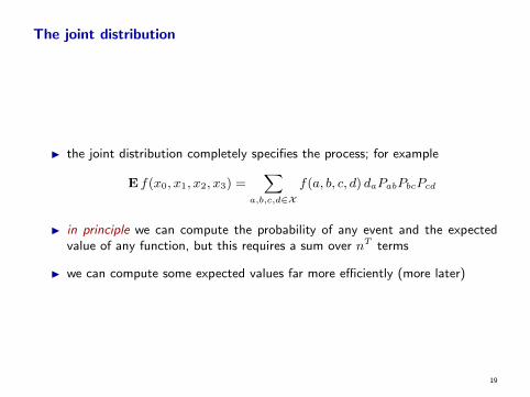
I the joint distribution completely specifies the process; for example
E f(x0, x1, x2, x3) =∑
a,b,c,d∈X
f(a, b, c, d) daPabPbcPcd
I in principle we can compute the probability of any event and the expectedvalue of any function, but this requires a sum over nT terms
I we can compute some expected values far more efficiently (more later)
19

Distribution Propagation
20

Distribution propagation
πt+1 = πtP
I here πt denotes distribution of xt, so
(πt)i = Prob(xt = i)
I can compute marginals π1, . . . , πT in Tn2 operations
I a useful type of simulation . . .
21

Example: Distribution propagation
0 1 2 3 4 5 6
p1p1p1p1p1
p0p0p0p0p0
p2p2p2p2p2
p0
p1
p2 p0
p1
p2
0 1 2 3 4 5 60
0.2
0.4
0.6
0.8
1
t = 0
0 1 2 3 4 5 60
0.2
0.4
0.6
0.8
1
t = 1
0 1 2 3 4 5 60
0.2
0.4
0.6
0.8
1
t = 2
0 1 2 3 4 5 60
0.2
0.4
0.6
0.8
1
t = 3
0 1 2 3 4 5 60
0.2
0.4
0.6
0.8
1
t = 4
0 1 2 3 4 5 60
0.2
0.4
0.6
0.8
1
t = 5
0 1 2 3 4 5 60
0.2
0.4
0.6
0.8
1
t = 9
0 1 2 3 4 5 60
0.2
0.4
0.6
0.8
1
t = 10
0 1 2 3 4 5 60
0.2
0.4
0.6
0.8
1
t = 20
22
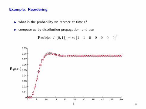
Example: Reordering
I what is the probability we reorder at time t?
I compute πt by distribution propagation, and use
Prob(xt ∈ 0, 1) = πt
[1 1 0 0 0 0 0
]T
0 5 10 15 20 25 30 35 40 45 500
0.01
0.02
0.03
0.04
0.05
0.06
0.07
0.08
0.09
E g(xt)
t 23
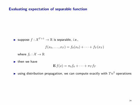
Evaluating expectation of separable function
I suppose f : X T+1 → R is separable, i.e.,
f(x0, . . . , xT ) = f0(x0) + · · ·+ fT (xT )
where ft : X → R
I then we haveE f(x) = π0f0 + · · ·+ πT fT
I using distribution propagation, we can compute exactly with Tn2 operations
24

Powers of the transition matrix
as an example of the use of the joint distribution, let’s show
(P k)ij = Prob(xt+k = j |xt = i
)this holds because
Prob(xt+k = st+k |xt = st
)=
Prob(xt+k = st+k and xt = st
)Prob
(xt = st
)
=
∑s0,s1,...,st−1,st+1,...,st+k−1
ds0Ps0s1Ps1s2 · · ·Pst+k−1st+k
Prob(xt = st
)
=
( ∑s0,s1,...,st−1
ds0Ps0s1 · · ·Pst−1st
)( ∑st+1,...,st+k−1
Pstst+1 · · ·Pst+k−1st+k
)Prob
(xt = st
)25
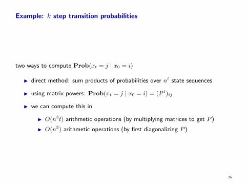
Example: k step transition probabilities
two ways to compute Prob(xt = j | x0 = i)
I direct method: sum products of probabilities over nt state sequences
I using matrix powers: Prob(xt = j | x0 = i) = (P t)ij
I we can compute this in
I O(n3t) arithmetic operations (by multiplying matrices to get P )
I O(n3) arithmetic operations (by first diagonalizing P )
26
Other Models
27
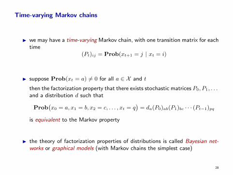
Time-varying Markov chains
I we may have a time-varying Markov chain, with one transition matrix for eachtime
(Pt)ij = Prob(xt+1 = j | xt = i)
I suppose Prob(xt = a) 6= 0 for all a ∈ X and t
then the factorization property that there exists stochastic matrices P0, P1, . . .and a distribution d such that
Prob(x0 = a, x1 = b, x2 = c, . . . , xt = q
)= da(P0)ab(P1)bc · · · (Pt−1)pq
is equivalent to the Markov property
I the theory of factorization properties of distributions is called Bayesian net-works or graphical models (with Markov chains the simplest case)
28

Dynamical system representation revisited
xt+1 = f(xt, wt)
If x0, w0, w1, . . . are independent then x0, x1, . . . is Markov
29

Dynamical system representation
To see that x0, x1, . . . is Markov, notice that
Prob(xt+1 = st+1 |x0 = s0, . . . , xt = st)
= Prob(f(st, wt) = st+1 |x0 = s0, . . . , xt = st
)= Prob
(f(st, wt) = st+1 |φt(x0, w0, . . . , wt−1) = (s0, . . . , st)
)= Prob
(f(st, wt) = st+1
)
I (x0, . . . , xt) = φt(x0, w0, . . . , wt−1) follows from xt+1 = f(xt, wt)
I last line holds since wt ⊥⊥ (x0, w0, . . . , wt−1) and x ⊥⊥ y =⇒ f(x) ⊥⊥ g(y)
x0, x1, . . . is Markov because the above approach also gives
Prob(xt+1 = st+1 |xt = st) = Prob(f(st, wt) = st+1
)30
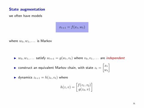
State augmentation
we often have models
xt+1 = f(xt, wt)
where w0, w1, . . . is Markov
I w0, w1, . . . satisfy wt+1 = g(wt, vt) where v0, v1, . . . are independent
I construct an equivalent Markov chain, with state zt =
[xtwt
]I dynamics zt+1 = h(zt, vt) where
h(z, v) =
[f(z1, z2)g(z2, v)
]
31
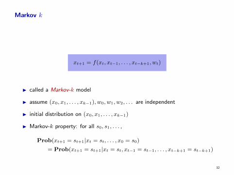
Markov k
xt+1 = f(xt, xt−1, . . . , xt−k+1, wt)
I called a Markov-k model
I assume (x0, x1, . . . , xk−1), w0, w1, w2, . . . are independent
I initial distribution on (x0, x1, . . . , xk−1)
I Markov-k property: for all s0, s1, . . . ,
Prob(xt+1 = st+1|xt = st, . . . , x0 = s0)
= Prob(xt+1 = st+1|xt = st, xt−1 = st−1, . . . , xt−k+1 = st−k+1)
32

Markov k
xt+1 = f(xt, xt−1, . . . , xt−k+1, wt)
I equivalent Markov system, with state zt ∈ Z = X k; notice that |Z| = |X |k
zt =
xtxt−1
...xt−k+1
I dynamics zt+1 = g(zt, wt) where
g(z, w) =
f(z1, z2, . . . , zk, w
)z1...
zk−1
33
Markov language models
I given text, construct a Markov k model by counting the frequency of wordsequences
I applications:
I run particle simulation to generate new text
I suggest correct spellings when spell checking
I optical character recognition
I finding similar documents in information retrieval
34

Example: Markov language models
I example: approximately 78,000 words, 8,200 unique
He wasnt true and disappointment that wouldnt be very old school song at
once it on the grayish white stone well have charlies work much to keep your
wand still had a mouse into a very scratchy whiskery kiss. Then yes yes. I
hope im pretty but there had never seen me what had to vacuum anymore
because its all right were when flint had shot up while uncle vernon around
the sun rose up to. Bill used to. Ron who to what he teaches potions one. I
suppose they couldnt think about it harry hed have found out that didnt trust
me all sorts of a letter which one by older that was angrier about what they
would you see here albus dumbledore it was very well get a rounded bottle
of everyone follows me an awful lot his face the minute. Well send you get
out and see professor snape. But it must have his sleeve. I am i think. Fred
and hermione and dangerous said finally. Uncle vernon opened wide open.
As usual everyones celebrating all hed just have caught twice. Yehll get out.
Well get the snitch yet no way up his feet.
35

Markov language models
I another example
Here on this paper. Seven bottles three are poison two are wine one will get
us through the corridors. Even better professor flitwick could i harry said the
boy miserably. Well i mean its the girls through one of them hardly daring to
take rons mind off his rocker said ron loudly. Shut up said ron sounding both
shocked and impressed. Id have managed it before and you should have done
so because a second later hermione granger telling a downright lie to a baked
potato when professor quirrell too the nervous young man made his way along
the floor in front of the year the dursleys were his only chance to beat you to
get past fluffy i told her you didnt say another word on the wall wiping sweat
off his nerves about tomorrow. Why should he yet harry couldnt help trusting
him. This is goyle said the giant turning his back legs in anger. For the food
faded from the chamber theyd just chained up. Oh no it isnt the same thing.
Harry who was quite clear now and gathering speed. The air became colder
and colder as they jostled their way through a crowd.
36