ee236c project report - university of california, …eda.ee.ucla.edu/mingao/docs/energy management...
TRANSCRIPT

EE236C PROJECT REPORT
Energy Management for EV Charge Station in Distributed Power System
Min Gao
Prof. Lieven Vandenberghe Spring 2012
1. Introduction
Most traditional power systems generate electricity by heat power plants, hydropower
plants and nuclear plants, which are all centralized large electricity generation facilities.
The benefits by doing so is obvious, i.e. it has fully-fledged automatic control method such
that safety of the grid could be ensured, would generate electricity with fixed
frequency(50Hz in Asia, Europe and 60Hz in North America) so as to maintain the
stability of the whole system and would have a low cost of every kWh of electricity.
However, traditional generation method is hard to achieve peak regulation nicely, would
lose lots of energy during long distance transmission and cause severe environmental issue.
On the other hand Distributed Power System(DPS) generates electricity from many small
energy sources. Using DPS could suit the need for the small area near where it has been
located, reduce the long distance transmission loss and eco-friendly since most of the
generation method would not produce as much pollution as the conventional one. The
major concern about DPS is the relatively poor electricity quality compared with the
traditional one. In most cases, power companies are reluctant to let power flow from DPS
sources flow into their stable power grids.
Since fossil fuels become more and more expensive and have been regarded as the main
issue for global warming, people started to find alternative ways to substitute fossil fuels.
With the merit of clean and cheap, electricity has become a good alternative in automobile
industry. Many automobile manufactures began to produce HEV and EV instead of
traditional cars.
Usually, Charging process for EV would be done in a charge station just like gas station
for normal vehicles. Since electricity generated by distributed generator might not satisfy
the need of electricity quality for the conventional power grid, a feasible solution is to
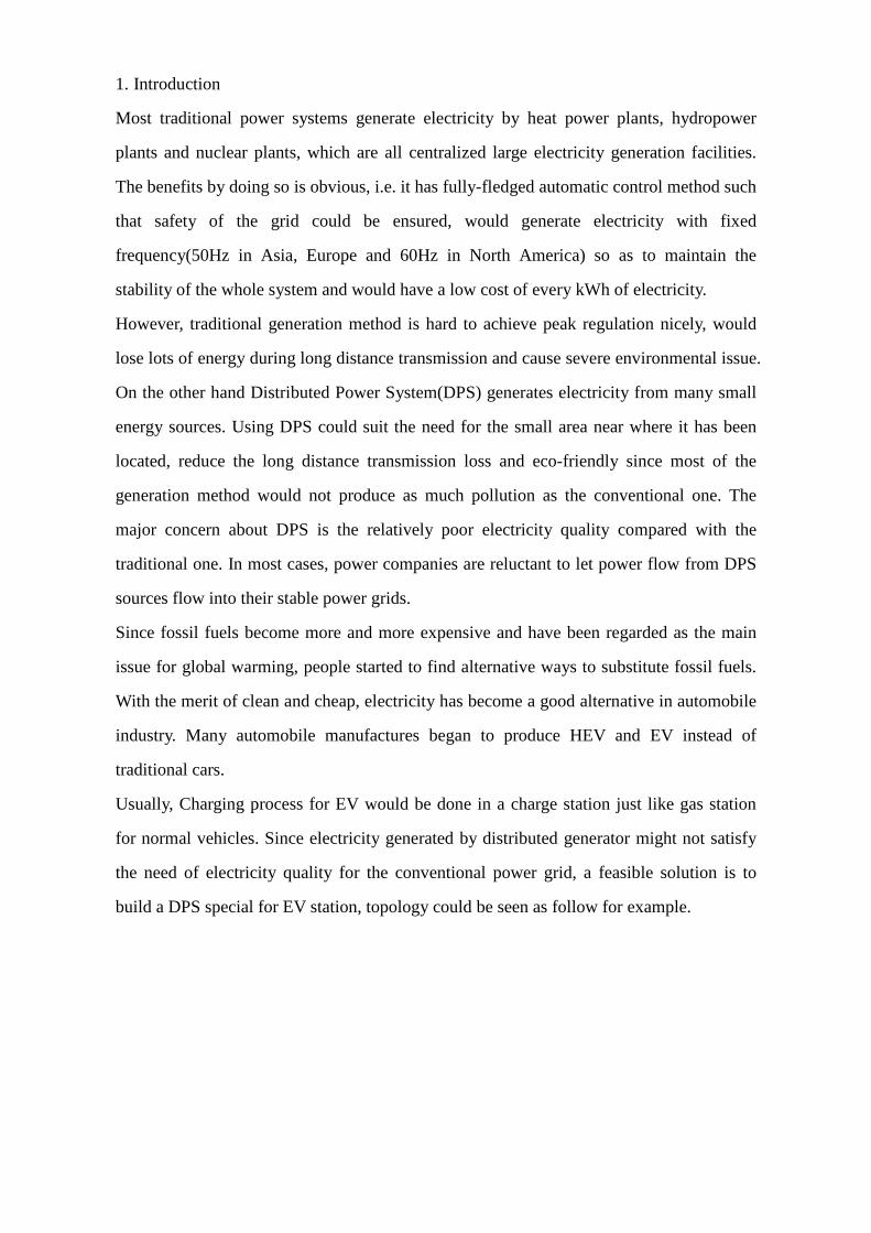
build a DPS special for EV station, topology could be seen as follow for example.
This topology is consist of few batteries which connected to the DPS generator, super
capacitors(or other energy storage device) which can be regarded as back up energy
storage and a switch connects to conventional grid in case of the total amount of the
generated electricity could not satisfy the need of the EV charge station. Typically
charging profile for a EV is a combination of constant current charging, constant voltage
charging and PWM controlled current charging.
Typically there are two different kinds of charging method. The first method would have
two charging stage. The first stage is to charge the battery at constant C-rate until it
reaches nominal voltage value, the second phase is to charge it at constant voltage until
charging current became 0.1 time of current value in the first stage. The second method is
to charge the battery with some pulse current and gradually decrease the charging current
when battery voltage reaches some threshold.
The performance of this topology would have a strong rely on batteries and other storage
device, thus an optimal electricity management method for this topology is of great
demand to be developed.
2. Model Formulation
In this problem, by given load current over time, capacity, SOC and other parameters of
batteries and super capacitors, we want to obtain an optimal battery and super capacitor
discharging schedule from distributed power source so as to prolong battery life and
Fig 1 Charging Station Topology
minimize the energy loss in a distributed generation based EV charging station.
We have following general assumptions. First is at high sample frequency, current/voltage
value between each time step is constant. Then the second one is conventional power grid
will only connected to super capacitors and charge them when needed. Third one is all the
battery and super capacitor current are dynamically control by power electronic device.
Other minor assumptions are described in detailed case.
2.1 Battery Life Optimization
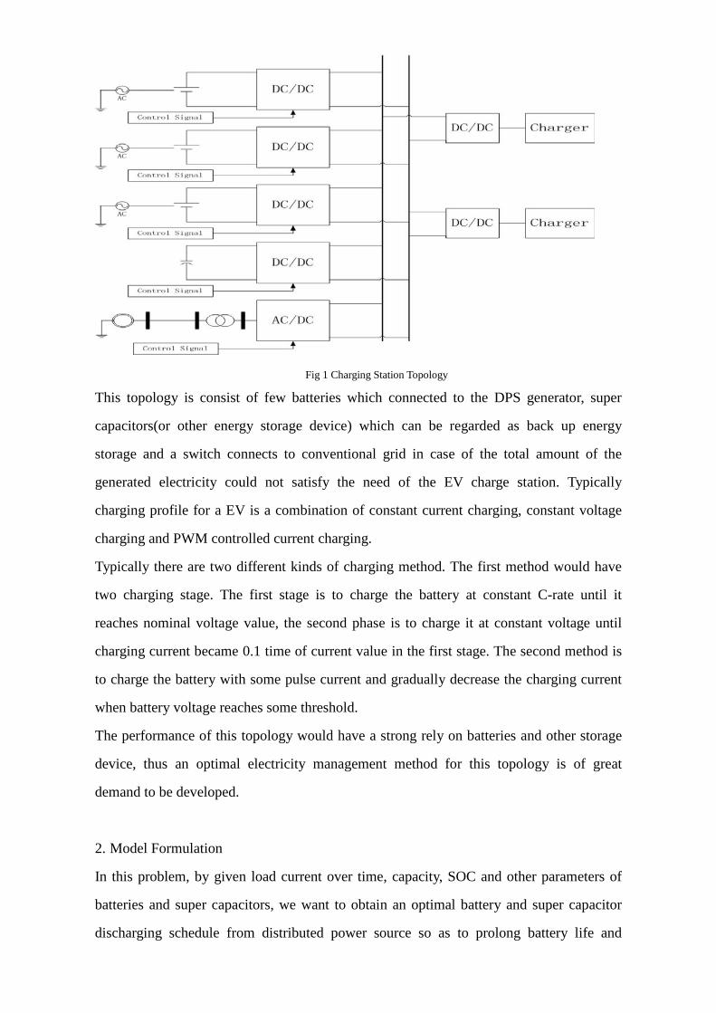
Generally for a battery, the higher the discharge rate is, the less the battery life will be. The
higher Depth of Discharge(DOD) of a battery is, the higher battery capacity degradation
will be.High current value would increase batteries' internal resistance more rapidly and
thus would make batteries' life become shorter. Also note that for certain given discharge
rate, battery cells which is cycled at high level DODs were shown to reach the defined end
of life, i.e. only 70% capacticy of a fresh battery could this battery be charged, much
sooner than those cycled at lower DODs (<50%). This observation is illustrated in Fig. 2
To achieve the goal of long battery life, we will control the current value flows through the
batteries and try to make it as small as possible, also we would like to control the
fluctuation of current value so as to make things easy for controller chips to control the
circuit.
We assume that the voltage and current are measured using discrete signals with a
sufficiently small sampling period . The battery has a capacity in amp-hour units.
The magnitude of the battery current and the current fluctuation of the battery can be
denoted as BI and |)1()(| −− tItI BB , respectively.
Fig 2 Battery Cycle Life VS DOD
For the whole discharging period, we want to minimize the summation of current at each
time step and summation of fluctuation, which is denoted as ∑∈Tt
B tI )(
and ∑∈−
−−Ttt
BB tItI1,
|)1()(| .
For each battery, we want the current flows out from it would not be greater than some
value but not strictly less than it. So a penalty function could play a role here to minimize
the objective and ensure most of the value would be less than desired value. In this
problem, we will choose Huber penalty function.
≥−<
=1||1||21||||
)(2
zzzz
zϕ
Since the Depth of Discharge is a great concern during the EV charging process, a SOC
lower bound for each battery will be added to ensure they will not be over-discharged.
Case1 Battery Only Topology with Identical Parameters
This might be the simplest case among all the possible topologies. The objective function
aims to make current as small as possible and tries deviate current fluctuation. The only
constraint might be Kirchhoff's Circuit Law which is the current flows out from the battery
should be equal to those flows into EV. The optimization problem is shown as below.
0)()(..
),|)1()((|),)((min
1
12
1,11
=+
−−+
∑∑
∑ ∑∑∑
∈=
= ∈−= ∈
Nnload
m
iB
m
i TttBB
m
i TtB
tItIts
tItItI
ni
iiiλϕλϕ
Where )),(( bxfϕ is huber penalty function
This is obviously a convex optimization problem.
Case2 Battery Only Topology with Different parameters
In this case the difference between the case1 is that each battery would have different
capacity and different initial SOC value. By doing so we could simulate each battery's
condition in a more practical manner. For the purpose of SOC balancing between each
battery so that we could fully use every battery and avoid the case that one of the battery
draines out but other batteries still remain plenty of charge, the objective function would
need to keep the difference of each battery's SOC in a small value besides achieveing the
functionality in case 1.
13.0
0)()(..
||||),|)1()((|),)((min
1
11
21,1
1
×≥
=+
+−−+
∑∑
∑ ∑∑∑
∈=
= ∈−= ∈
G
tItIts
FGtItItI
Nnload
m
iB
m
i TttBB
m
i TtB
ni
iiiλϕλϕ
where
)(
))()()(()(
110000......0000......000011
iQ
ttIisociQiG
F
TtBi ∆×−
=
−
−
=
∑∈
In the formulation above, F is teoplitz matrix and G represents for SOC of each battery at
every time step. The second constraint means that DOD for every battery should not be
greater than 70% which is aiming to prolong the battery life. This is also a convex
programming problem.
Case3 Battery and Super Capacitor Topology
Fig 3 is the equivalent circuit for super Capacitors. Denote terminal voltage, capacitor
current, equivalent serial resistance(ESR), and capacitance as ksss CRivkkk,,, respectfully.
From basic circuit theory we have
dttiC
tvTt
sk
s kk)(1)( ∫
∈
−=
One benefit for us to use super capacitor is that it could accept huge current change
between time steps and this will provide the possibility to make battery current have less
fluctuations.
Here we also assume that that the initial capacitor voltage should remain the same to the
Fig 3 Super Capacitor Equivalent Circuit
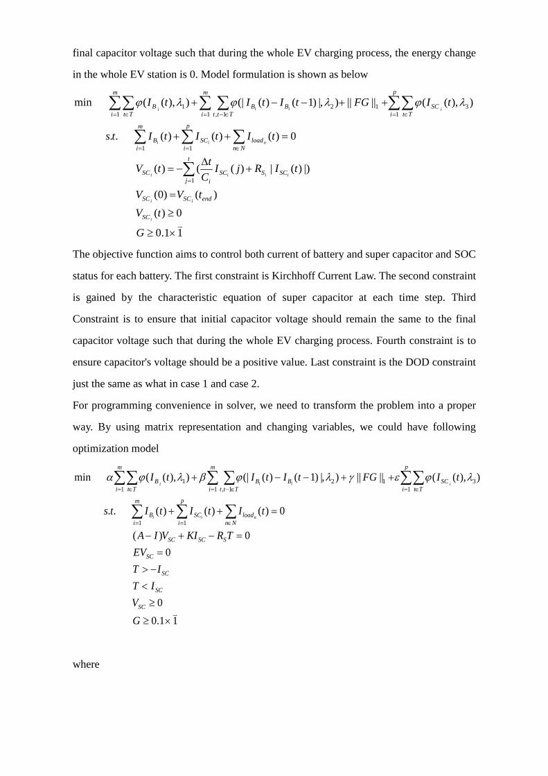
final capacitor voltage such that during the whole EV charging process, the energy change
in the whole EV station is 0. Model formulation is shown as below
11.0
0)(
)()0(
|))(|)(()(
0)()()(..
),)((||||),|)1()((|),)((min
1
11
131
12
1,11
×≥
≥
=
+∆
−=
=++
++−−+
∑
∑∑∑
∑∑∑ ∑∑∑
=
∈==
= ∈= ∈−= ∈
G
tV
tVV
tIRjIC
ttV
tItItIts
tIFGtItItI
i
ii
iiii
nii
iiii
SC
endSCSC
t
jSCSSC
iSC
Nnload
p
iSC
m
iB
p
i TtSC
m
i TttBB
m
i TtB λϕλϕλϕ
The objective function aims to control both current of battery and super capacitor and SOC
status for each battery. The first constraint is Kirchhoff Current Law. The second constraint
is gained by the characteristic equation of super capacitor at each time step. Third
Constraint is to ensure that initial capacitor voltage should remain the same to the final
capacitor voltage such that during the whole EV charging process. Fourth constraint is to
ensure capacitor's voltage should be a positive value. Last constraint is the DOD constraint
just the same as what in case 1 and case 2.
For programming convenience in solver, we need to transform the problem into a proper
way. By using matrix representation and changing variables, we could have following
optimization model
11.00
00)(
0)()()(..
),)((||||),|)1()((|),)((min
11
131
12
1,11
×≥
≥<−>=
=−+−
=++
++−−+
∑∑∑
∑∑∑ ∑∑∑
∈==
= ∈= ∈−= ∈
GV
ITIT
EVTRKIVIA
tItItIts
tIFGtItItI
SC
SC
SC
SC
SSCSC
Nnload
p
iSC
m
iB
p
i TtSC
m
i TttBB
m
i TtB
nii
iiiiλϕεγλϕβλϕα
where
)(
))()()(()(
110000......0000......000011
]1,0,...,0,0,1[
0
00]0,...,0,1[
iQ
ttIisociQiG
F
EI
tK
IA
TtB
n
n
i∑∈
∆×−=
−
−
=
−=
∆=
=
Matrix A comes from processing with one time step and the next time step of the
constraint of super capacity voltage recursively. This formulation is obviously a convex
optimization problem.
Note that with some high current value, first two huber penalty function would return
significant large value which will lower the influence of other terms. We would put some
weight to all the components to adjust this phenomenon.
2.2 Energy Loss Optimization
In EV charging station system, energy loss from power side is mainly generated by
equivalent serial resistance in super capacitors. Especially during the charging and
discharging of the SCs. Although an energy loss can be induced by the battery since it also
has internal resistance, we will ignore it because resistance in battery is relatively small
compared to ESR in super capacitors.
Denote Power loss as lossQ and ∫= tRtIQloss d)( 2 . In problem formulation, we will
simply use RttI )( instead of lossQ to make calculation easier since minimize these two
functions with the same constraint would return the same optimal solution.
The optimization model is shown as follows, the only difference between this formulation
and previous one is the change in objective function.
11.00
00)(
0)()()(..
min
11
×≥
≥<−>=
=−+−
=++
∆××
∑∑∑∈==
GV
ITIT
EVTRKIVIA
tItItIts
tIR
SC
SC
SC
SC
SSCSC
Nnload
p
iSC
m
iB
SCs
nii
2.3 Multi-criteria Formulation
Two objectives mentioned above are needed to be considered simultaneously, i.e., the
minimization of magnitude and fluctuation for battery and minimization of total energy
loss. A combined formulation is shown as follows
11.0
0
00)(
0)()()(..
),)((||||),|)1()((|),)((min
11
131
12
1,11
×≥
≥<−>=
=−+−
=++
∆+++−−+
∑∑∑
∑∑∑ ∑∑∑
∈==
= ∈= ∈−= ∈
GV
ITIT
EVTRKIVIA
tItItIts
tIRtIFGtItItI
SC
SC
SC
SC
SSCSC
Nnload
p
iSC
m
iB
p
iSCs
TtSC
m
i TttBB
m
i TtB
nii
iiiiµλϕεγλϕβλϕα
where
)(
))()()(()(
110000......0000......000011
]1,0,...,0,0,1[
0
00]0,...,0,1[
iQ
ttIisociQiG
F
EI
tK
IA
TtB
n
n
i∑∈
∆×−=
−
−
=
−=
∆=
=
3. Numerical Result
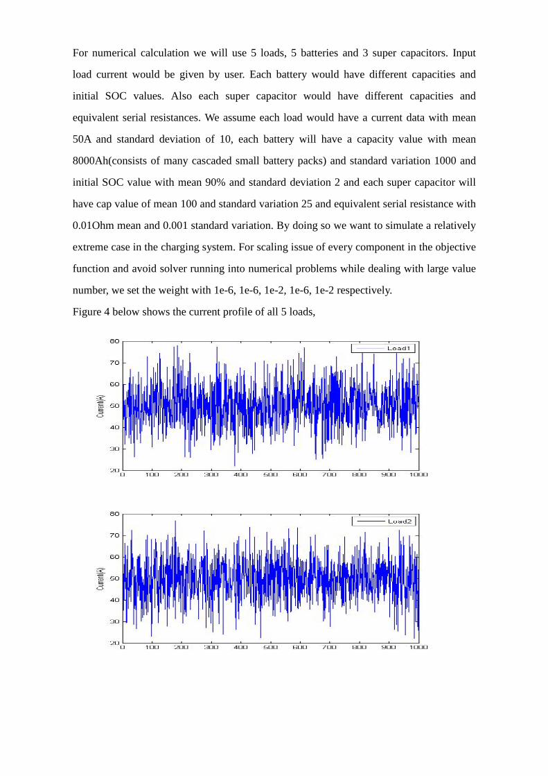
For numerical calculation we will use 5 loads, 5 batteries and 3 super capacitors. Input
load current would be given by user. Each battery would have different capacities and
initial SOC values. Also each super capacitor would have different capacities and
equivalent serial resistances. We assume each load would have a current data with mean
50A and standard deviation of 10, each battery will have a capacity value with mean
8000Ah(consists of many cascaded small battery packs) and standard variation 1000 and
initial SOC value with mean 90% and standard deviation 2 and each super capacitor will
have cap value of mean 100 and standard variation 25 and equivalent serial resistance with
0.01Ohm mean and 0.001 standard variation. By doing so we want to simulate a relatively
extreme case in the charging system. For scaling issue of every component in the objective
function and avoid solver running into numerical problems while dealing with large value
number, we set the weight with 1e-6, 1e-6, 1e-2, 1e-6, 1e-2 respectively.
Figure 4 below shows the current profile of all 5 loads,
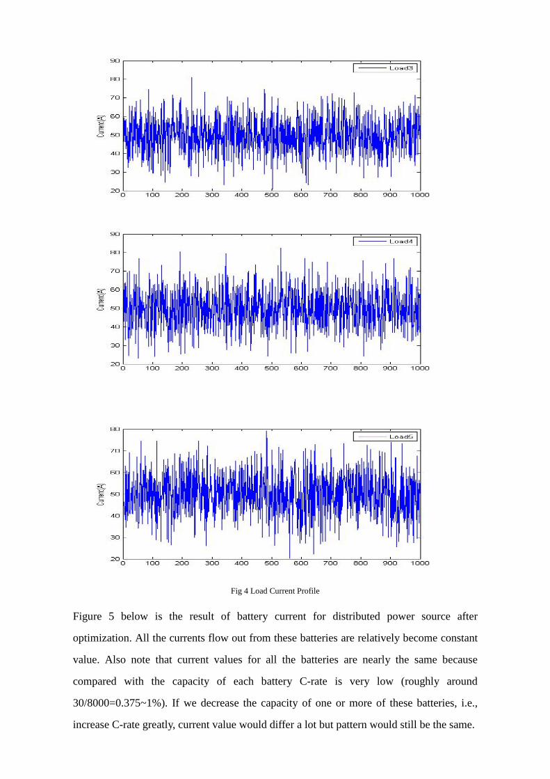
Figure 5 below is the result of battery current for distributed power source after
optimization. All the currents flow out from these batteries are relatively become constant
value. Also note that current values for all the batteries are nearly the same because
compared with the capacity of each battery C-rate is very low (roughly around
30/8000=0.375~1%). If we decrease the capacity of one or more of these batteries, i.e.,
increase C-rate greatly, current value would differ a lot but pattern would still be the same.
Fig 4 Load Current Profile
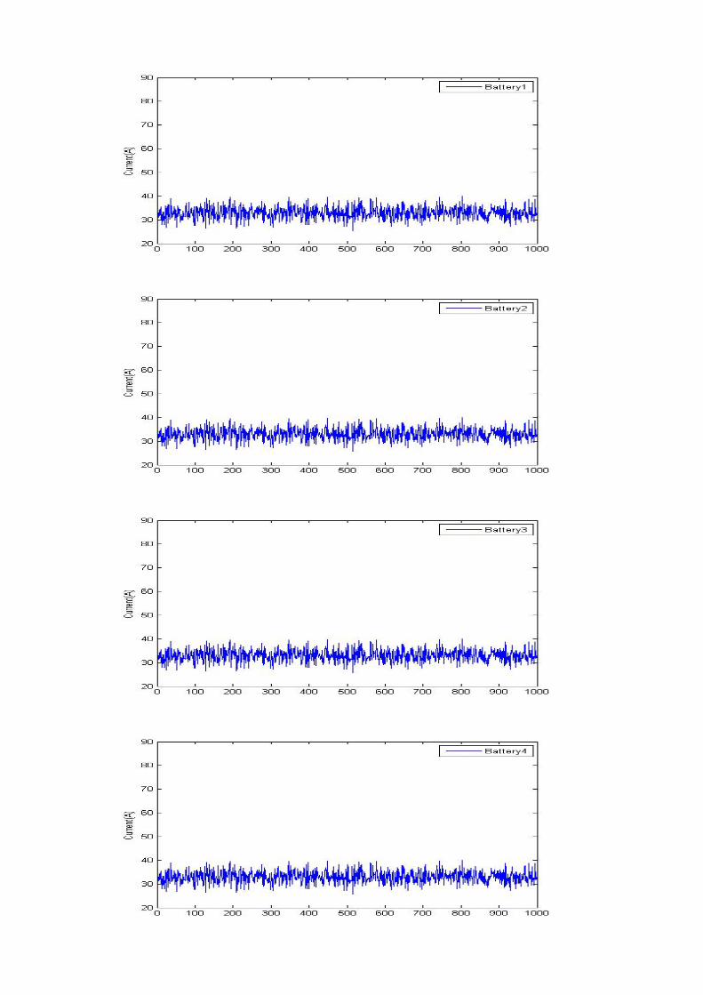
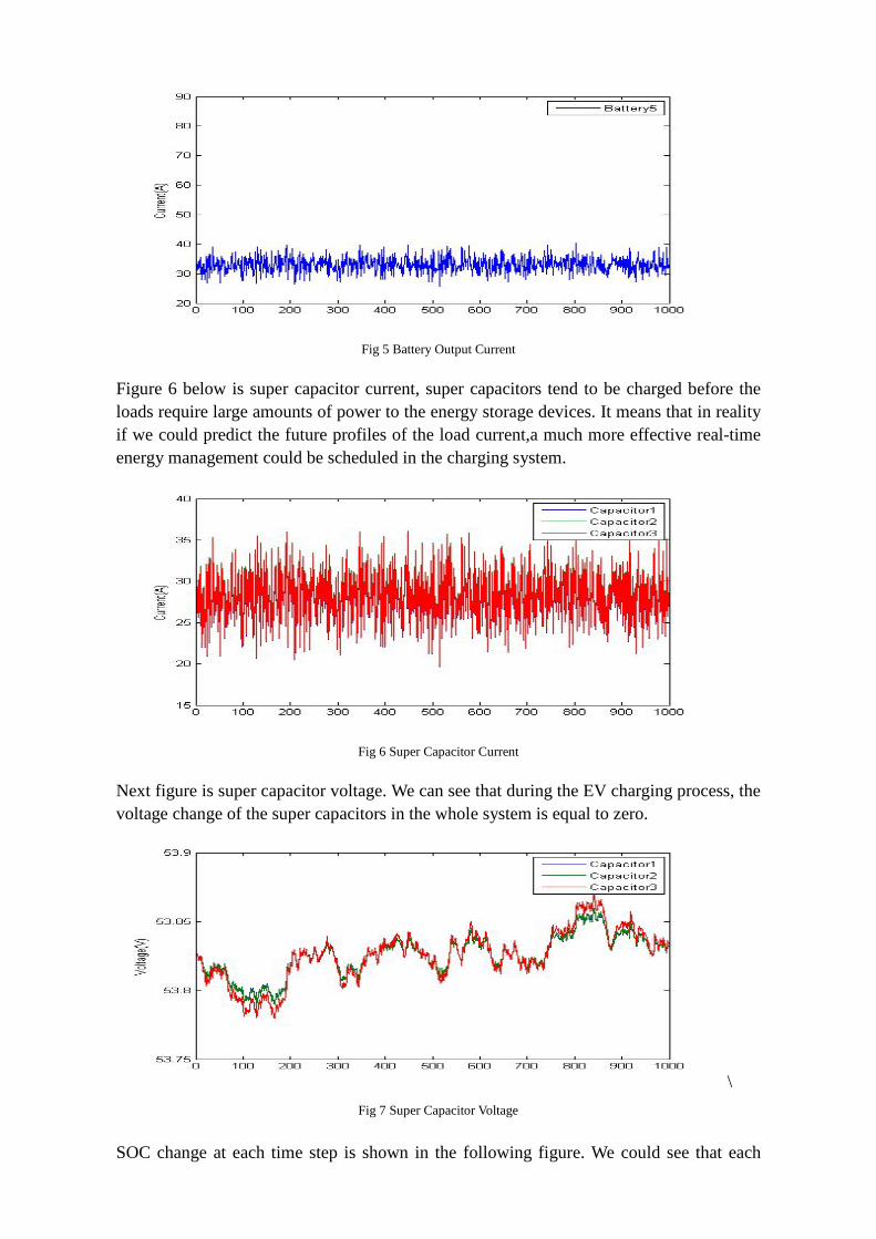
Figure 6 below is super capacitor current, super capacitors tend to be charged before the loads require large amounts of power to the energy storage devices. It means that in reality if we could predict the future profiles of the load current,a much more effective real-time energy management could be scheduled in the charging system.
Next figure is super capacitor voltage. We can see that during the EV charging process, the voltage change of the super capacitors in the whole system is equal to zero.
\
SOC change at each time step is shown in the following figure. We could see that each
Fig 5 Battery Output Current
Fig 6 Super Capacitor Current
Fig 7 Super Capacitor Voltage
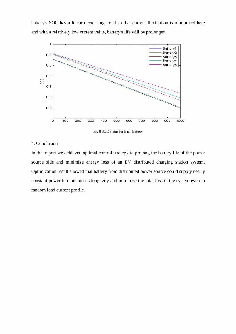
Fig 8 SOC Status for Each Battery
battery's SOC has a linear decreasing trend so that current fluctuation is minimized here
and with a relatively low current value, battery's life will be prolonged.
4. Conclusion
In this report we achieved optimal control strategy to prolong the battery life of the power
source side and minimize energy loss of an EV distributed charging station system.
Optimization result showed that battery from distributed power source could supply nearly
constant power to maintain its longevity and minimize the total loss in the system even in
random load current profile.
Reference
1. S. Boyd and L. Vandenberghe, Convex Optimization. Cambridge, U.K.,: Cambridge Univ. Press,
2004.
2. S.M. Lukic, S.G. Wirasinga, F. Rodriguez, J. Cao, and A. Emadi, "Power Mangement of an
Ultracapacitor/Battery Hybrid Energy Storage System in an HEV," in IEEE Veh. Power Prop. Conf.,
Sep. 2006, pp.1-6.
3. J. Wang, P. Liu, J. Hicks-Garner, E. Sherman, S. Soukiazian, M. Verbrugge, H. Tatariab, J. Musserc,
and P. Finamorec, "Cycle-life model for graphite-LiFePO4 cells,"Journal of Power Sources, vol. 96,
issue 8, pp 3942-8, Apr. 2011.
4. C. Cho, J. Jeon, J. Kim, S. Kwon, K. Park, S. Kim, "Active Synchronizing Control of a Microgrid",
Power Electronics, IEEE Transactions on, vol. 26, issue: 12, pp 3707 - 19 Dec. 2011.
5. Y. Zhang, Z. Jiang, and X. Yu, "Control Strategies for Battery/Super Capacitor Hybrid Energy
Storage Systems, " in Proc. IEEE Energy 2010 Conf., Nov. 2008, pp 1-6.
%%%%%%%%%%%%%%%%%%%%%%%%%%%%%%%%%%%%%%%%%%%%%%%%%%%%%%%% % %EV Charging Station Modeling %Multi-object function is now working %Could also comment out other cases to see result of such easier case %%%%%%%%%%%%%%%%%%%%%%%%%%%%%%%%%%%%%%%%%%%%%%%%%%%%%%%% clear all clc %%Initialization %n=1000sample points; %m=5battery %p=2 m=5; n=1000; k=4; p=2; C=zeros(1,n-1);C(1)=1; R=zeros(1,n);R(1)=1;R(2)=-1; M=zeros(1,m-1);M(1)=1; P=zeros(1,m); P(1)=1;P(2)=-1; T=toeplitz(C,R);F=toeplitz(M,P); Iload=normrnd(50,10,5,n); % %%Case1 % cvx_begin % variable Ibattery(m,n); % minimize (sum(sum(huber(Ibattery,70)))+sum(sum(huber(T*Ibattery',3)))) % subject to % %KCL % for i=1:n % sum(Ibattery(:,i))-sum(Iload(:,i))==0; % end % cvx_end % %%Case2 % capacity=normrnd(8000,1000,1,m); % soc=normrnd(90,6,1,m); % while (max(soc)>100 || min(soc)<0) % soc=normrnd(90,6,1,m); % end % Q=capacity.*soc/100; % for i=1:m % Sigma(i,:)=capacity(i)*0.01*ones(1,n); % end % % cvx_begin % variable Ibattery(m,n); % minimize
(sum(sum(huber(Ibattery,Sigma)/1e6))+sum(sum(huber(T*Ibattery',5)/1e6))+norm(F*((Q-sum(Ibattery')
*0.1)./Q)',1)) % subject to % %KCL % for i=1:n % sum(Ibattery(:,i))-sum(Iload(:,i))==0; % end % (Q-sum(Ibattery')*0.1)./Q>=0.1*ones(1,m); % cvx_end % Case3_1
% capacity=normrnd(8000,1000,1,m); % soc=normrnd(90,6,1,m); % while (max(soc)>100 || min(soc)<0) % soc=normrnd(90,6,1,m); % end % Q=capacity.*soc/100; % for i=1:m % Sigma(i,:)=capacity(i)*0.01*ones(1,n); % end % A=[1,zeros(1,n);eye(n),zeros(n,1)]; % I=eye(n+1); % K=0.1/100*[zeros(1,n);eye(n)]; % Rs=0.001*[zeros(1,n);eye(n)]; % E=[1,zeros(1,n-1),-1]; % % cvx_begin % variables Ibattery(m,n) Icapacity(1,n) Vcapacity(n+1) t(1,n); % minimize
(0.15*sum(sum(huber(Ibattery,65)/1e6))+0.5*sum(sum(huber(T*Ibattery',5)/1e6))+0.25*norm(F*((Q-sum
(Ibattery')*0.1)./Q)',1)+0.1*sum(sum(huber(Icapacity,120)/1e6))) % subject to % for i=1:n % sum(Ibattery(:,i))+sum(Icapacity(:,i))-sum(Iload(:,i))==0; % end % (A-I)*Vcapacity-K*Icapacity'-Rs*t'==0; % E*Vcapacity==0; % % t<Icapacity; % t>-Icapacity; % % (Q-sum(Ibattery')*0.1)./Q>=0.1*ones(1,m); % cvx_end %Case3_2 % mC=3; % capacity=normrnd(8000,1000,1,m); % soc=normrnd(90,6,1,m); % while (max(soc)>100 || min(soc)<0) % soc=normrnd(90,6,1,m); % end % Q=capacity.*soc/100; % for i=1:m % Sigma(i,:)=capacity(i)*0.01*ones(1,n); % end % A=[1,zeros(1,n);eye(n),zeros(n,1)]; % I=eye(n+1); % K=0.1*[zeros(1,n);eye(n)]; % scCapacity=normrnd(100,3,1,mC); % G=[zeros(1,n);eye(n)]; % Rs=normrnd(1,0.1,1,mC) % E=[1,zeros(1,n-1),-1]; % % cvx_begin % variables Ibattery(m,n) Icapacity(mC,n) Vcapacity(n+1,mC) t(mC,n); % minimize
(0.15*sum(sum(huber(Ibattery,65)/1e6))+0.5*sum(sum(huber(T*Ibattery',5)/1e6))+0.25*norm(F*((Q-sum
(Ibattery')*0.1)./Q)',1)+0.1*sum(sum(huber(Icapacity,120)/1e6))) % subject to % %KCL % for i=1:n % sum(Ibattery(:,i))+sum(Icapacity(:,i))-sum(Iload(:,i))==0; % end % for j=1:mC
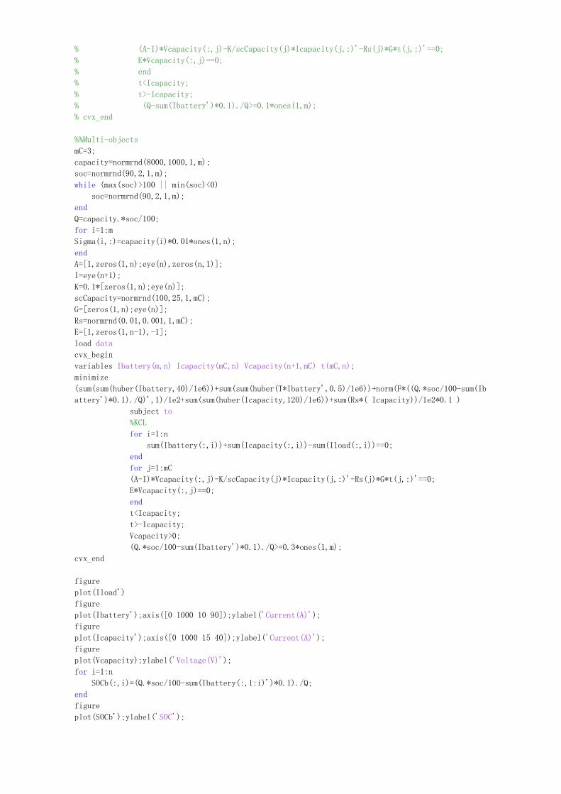
% (A-I)*Vcapacity(:,j)-K/scCapacity(j)*Icapacity(j,:)'-Rs(j)*G*t(j,:)'==0; % E*Vcapacity(:,j)==0; % end % t<Icapacity; % t>-Icapacity; % (Q-sum(Ibattery')*0.1)./Q>=0.1*ones(1,m); % cvx_end %%Multi-objects mC=3; capacity=normrnd(8000,1000,1,m); soc=normrnd(90,2,1,m); while (max(soc)>100 || min(soc)<0) soc=normrnd(90,2,1,m); end Q=capacity.*soc/100; for i=1:m Sigma(i,:)=capacity(i)*0.01*ones(1,n); end A=[1,zeros(1,n);eye(n),zeros(n,1)]; I=eye(n+1); K=0.1*[zeros(1,n);eye(n)]; scCapacity=normrnd(100,25,1,mC); G=[zeros(1,n);eye(n)]; Rs=normrnd(0.01,0.001,1,mC); E=[1,zeros(1,n-1),-1]; load data cvx_begin variables Ibattery(m,n) Icapacity(mC,n) Vcapacity(n+1,mC) t(mC,n); minimize
(sum(sum(huber(Ibattery,40)/1e6))+sum(sum(huber(T*Ibattery',0.5)/1e6))+norm(F*((Q.*soc/100-sum(Ib
attery')*0.1)./Q)',1)/1e2+sum(sum(huber(Icapacity,120)/1e6))+sum(Rs*( Icapacity))/1e2*0.1 ) subject to %KCL for i=1:n sum(Ibattery(:,i))+sum(Icapacity(:,i))-sum(Iload(:,i))==0; end for j=1:mC (A-I)*Vcapacity(:,j)-K/scCapacity(j)*Icapacity(j,:)'-Rs(j)*G*t(j,:)'==0; E*Vcapacity(:,j)==0; end t<Icapacity; t>-Icapacity; Vcapacity>0; (Q.*soc/100-sum(Ibattery')*0.1)./Q>=0.3*ones(1,m); cvx_end figure plot(Iload') figure plot(Ibattery');axis([0 1000 10 90]);ylabel('Current(A)'); figure plot(Icapacity');axis([0 1000 15 40]);ylabel('Current(A)'); figure plot(Vcapacity);ylabel('Voltage(V)'); for i=1:n SOCb(:,i)=(Q.*soc/100-sum(Ibattery(:,1:i)')*0.1)./Q; end figure plot(SOCb');ylabel('SOC');