ee2090 – basic engineering mathematics assoc. prof. m - webs
TRANSCRIPT

EE2090 – Basic EngineeringMathematics
Assoc. Prof. M. AdamsRoom : S2.2-B2-23
Extn : 4361Email : [email protected]
TOPICS
1. Multiple Integrals
2. Infinite Sequences & Series
3. Vectors
4. Introduction to Laplace Transforms
EE2090 – Basic Engineering Mathematicsslide-1

Recommended Text Books
Text:
1. Gerald L. Bradley & K.J. Smith, “Calculus”, 3rd Edition, Prentice
Hall.
2. Erwin Kreyzig, “Advanced Engineering Mathematics, 8th Edition,
John Wiley, 1999.
EE2090 – Basic Engineering Mathematicsslide-2

Course Contents
Multiple Integrals
1. Double Integrals
(a) Regions of Integration
(b) Iterated Integrals
(c) Double Integrals in Polar Coordinates
2. Triple Integrals
Infinite Sequences & Series
1. Sequences and Series
2. Convergence and Tests for Convergence
Vectors
1. Vectors in the Plane
2. Dot and Cross product
3. Lines and Planes in Space
4. Vector Methods for Measuring Distance in R3
EE2090 – Basic Engineering Mathematicsslide-3
Course Contents
Laplace Transforms
1. Definition
(a) Linearity
(b) Inverse Laplace Transform
2. Properties of Laplace Transforms
(a) Differentiation
(b) Integration
(c) Shifting on the s-axis
(d) Shifting on the t-axis
EE2090 – Basic Engineering Mathematicsslide-4

EE2090 2004/05
MULTIPLE INTEGRALS
We shall examine
• Double Integrals, and
• Triple Integrals
First, the Double Integrals
The Double Integral of f over the region R is
4

EE2090 2004/05∫ ∫R
f(x, y)dA = limm,n→∞
m∑i=1
n∑j=1
f(x∗ij, y∗ij)∆A
if this limit exists.
To understand this, let’s review the familiar Definite Integral:
5

EE2090 2004/05
If f(x) is defined for a ≤ x ≤ b, then
b∫a
f(x)dx = limn→∞
n∑i=1
f(x∗i )∆x
• Divide interval [a, b] into n subintervals [xi−1, xi];
• ∆x = (b− a)/n;
6

EE2090 2004/05
• x∗i are sample points in the subintervals;
• Riemann sum is
n∑i=1
f(x∗i )∆x
• Taking the limit of such sum as n → ∞ to obtain the definite
integral of f from a to b !
• The integral represents the area under the curve y = f(x) from
a to b
7

EE2090 2004/05
Volumes and Double Integrals
In a similar manner, we consider:
8
EE2090 2004/05
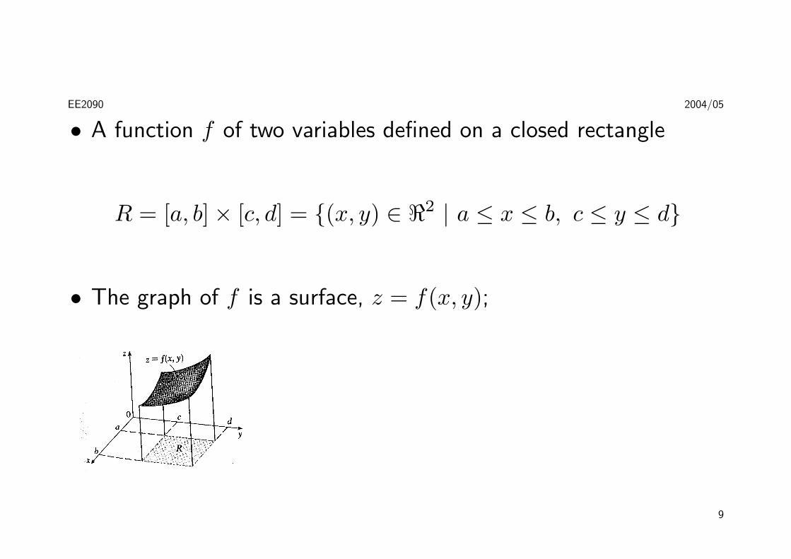
• A function f of two variables defined on a closed rectangle
R = [a, b]× [c, d] = {(x, y) ∈ <2 | a ≤ x ≤ b, c ≤ y ≤ d}
• The graph of f is a surface, z = f(x, y);
9

EE2090 2004/05
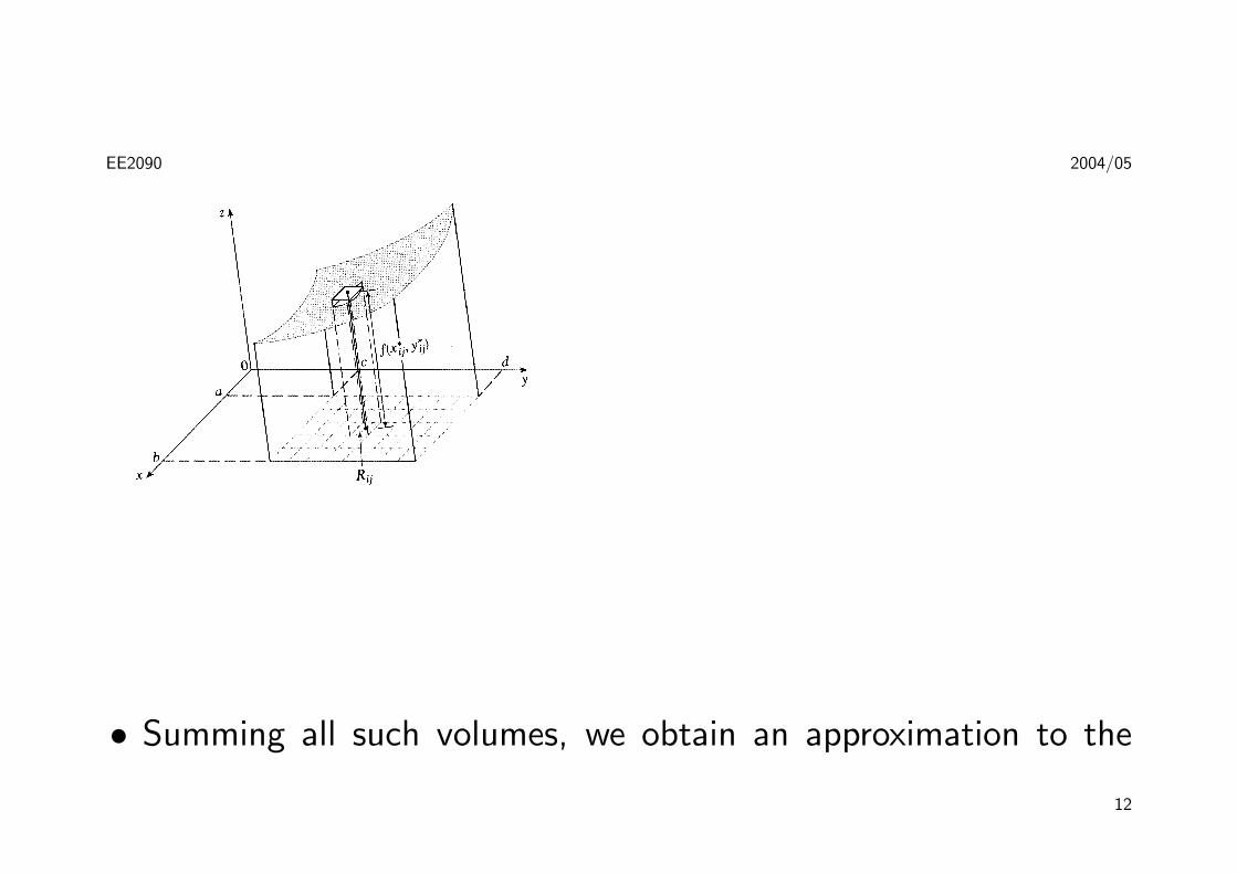
• Let S be the solid that lies above R and under the graph of f :
S = {(x, y, z) ∈ <3 | 0 ≤ z ≤ f(x, y), (x, y) ∈ R}
• Divide the rectangle R into m× n subrectangles;
10

EE2090 2004/05
• ∆x = (b− a)/m and ∆y = (d− c)/n;
• Area of subrectangle Rij is ∆A = ∆x∆y;
• Choose a sample point (x∗ij, y∗ij) in each Rij;
• Volume of the thin column with base Rij and height f(x∗ij, y∗ij) is
f(x∗ij, y∗ij)∆A
11
EE2090 2004/05
• Summing all such volumes, we obtain an approximation to the
12
EE2090 2004/05
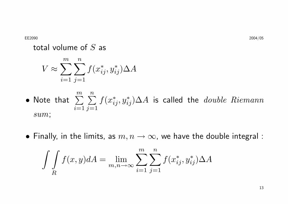
total volume of S as
V ≈m∑
i=1
n∑j=1
f(x∗ij, y∗ij)∆A
• Note thatm∑
i=1
n∑j=1
f(x∗ij, y∗ij)∆A is called the double Riemann
sum;
• Finally, in the limits, as m,n →∞, we have the double integral :∫ ∫R
f(x, y)dA = limm,n→∞
m∑i=1
n∑j=1
f(x∗ij, y∗ij)∆A
13

EE2090 2004/05
• Note, taking the sample point as (xi, yj) gives
∫ ∫R
f(x, y)dA = limm,n→∞
m∑i=1
n∑j=1
f(xi, yj)∆A
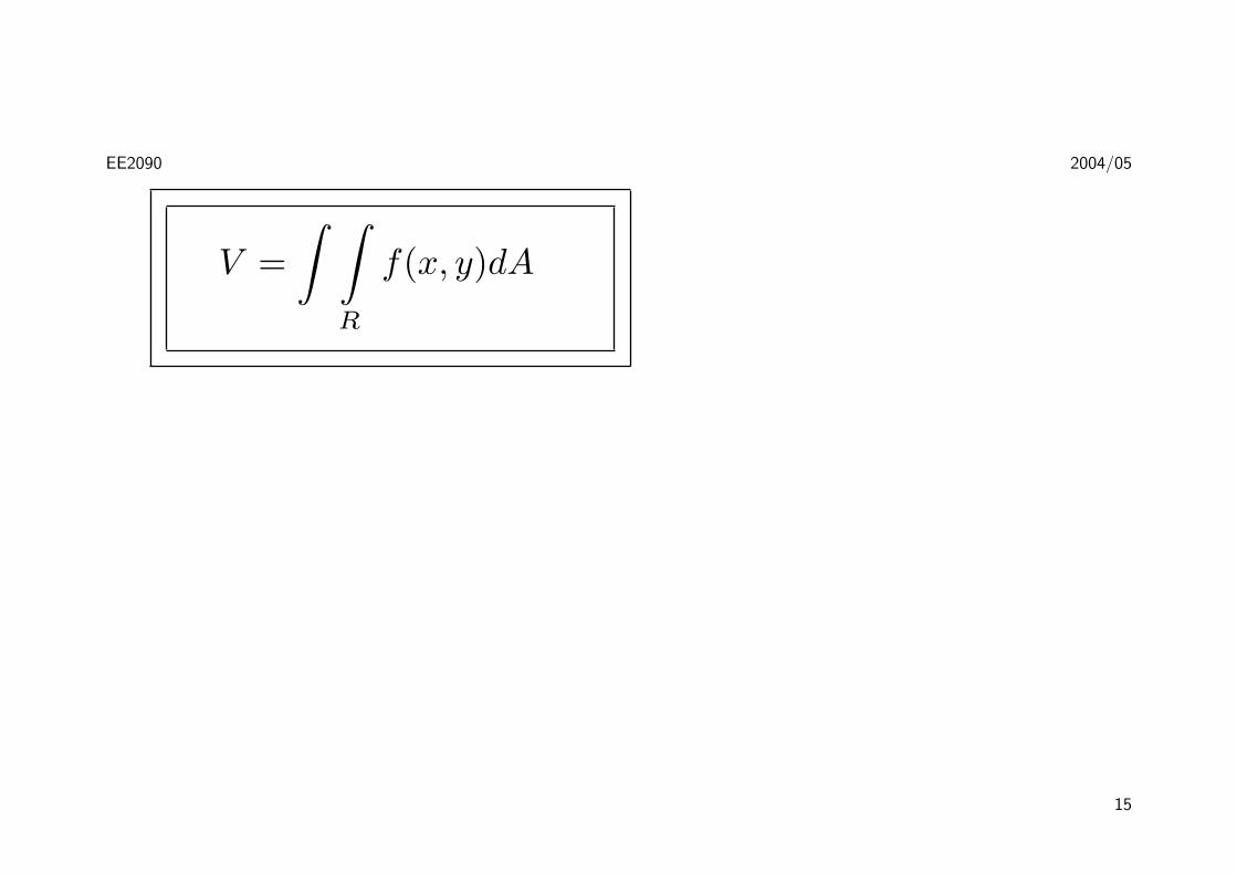
A volume can thus be written as a double integral:
14
EE2090 2004/05
V =∫ ∫
R
f(x, y)dA
15

EE2090 2004/05
Iterated Integrals
• It is usually very difficult to evaluate double integrals from first
principle!
• A practical method for evaluating a double integral is by expressing
it as an iterated integral.
• Suppose f is a function of two variables, continuous on the
rectangle R = [a, b]× [c, d]
16
EE2090 2004/05
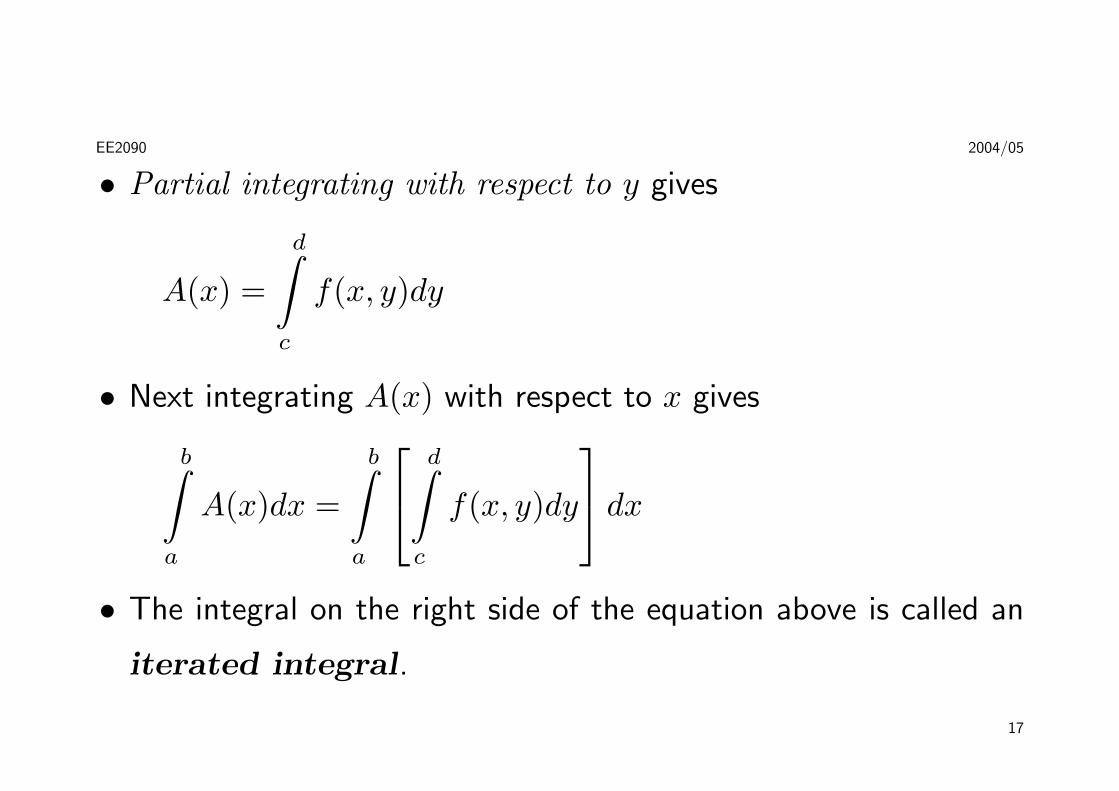
• Partial integrating with respect to y gives
A(x) =
d∫c
f(x, y)dy
• Next integrating A(x) with respect to x gives
b∫a
A(x)dx =
b∫a
d∫c
f(x, y)dy
dx
• The integral on the right side of the equation above is called an
iterated integral.
17

EE2090 2004/05
• Using the iterated integral, we can now express a double integral as
∫ ∫R
f(x, y)dA =
b∫a
d∫c
f(x, y)dydx =
d∫c
b∫a
f(x, y)dxdy
• Note that the order of integration does not matter.
18
EE2090 2004/05
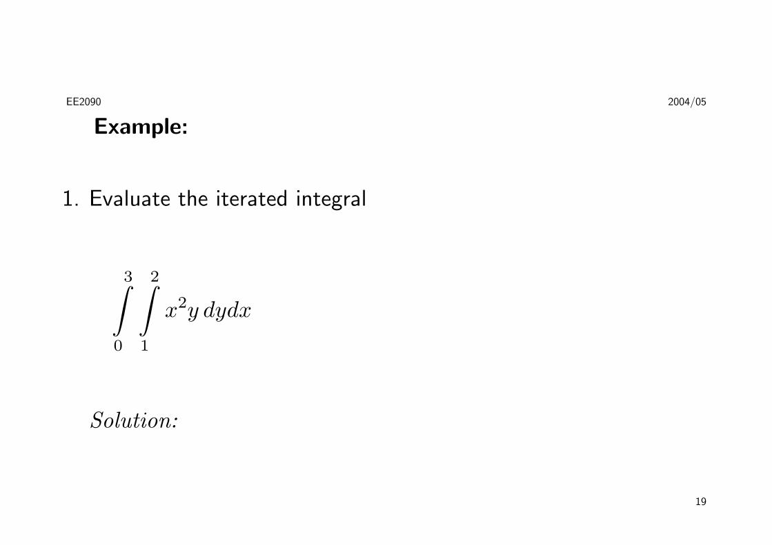
Example:
1. Evaluate the iterated integral
3∫0
2∫1
x2y dydx
Solution:
19
EE2090 2004/05
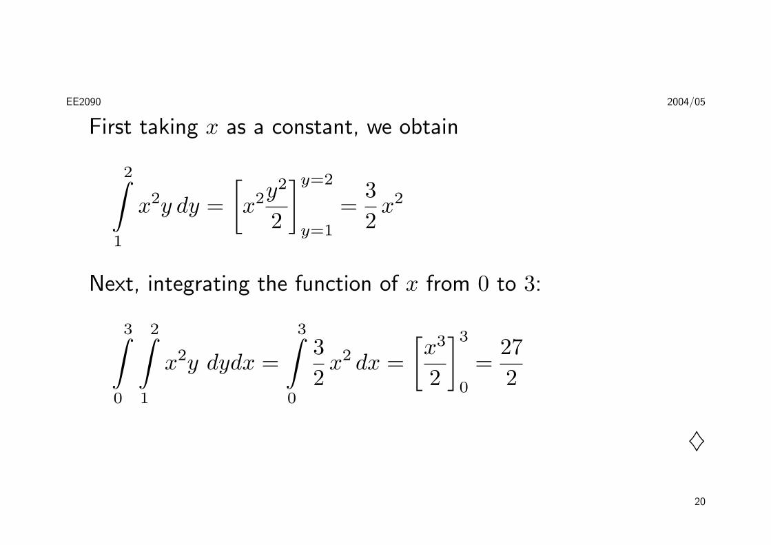
First taking x as a constant, we obtain
2∫1
x2y dy =[x2y
2
2
]y=2
y=1
=32
x2
Next, integrating the function of x from 0 to 3:
3∫0
2∫1
x2y dydx =
3∫0
32
x2 dx =[x3
2
]3
0
=272
♦
20
EE2090 2004/05
2. Evaluate the double integral∫ ∫R
(x− 3y2) dA
where R = {(x, y) | 0 ≤ x ≤ 2, 1 ≤ y ≤ 2}.
Solution:
∫ ∫R
(x− 3y2)dA =
2∫0
2∫1
(x− 3y3) dy dx
21
EE2090 2004/05
=∫ 2
0
[xy − y3
]y=2
y=1dx
=
2∫0
(x− 7) dx =x2
2− 7x
]2
0
= −12
♦
3. Evaluate∫ ∫
Ry sin(xy) dA, where R = [1, 2]× [0, π].
22

EE2090 2004/05
Solution:
∫ ∫R
y sin(xy) dA =
π∫0
2∫1
y sin(xy) dxdy
=
π∫0
[− cos(xy)]x=2x=1 dy
=
π∫0
(− cos 2y + cos y) dy
23
EE2090 2004/05
= −12
sin 2y + sin y
]π
0
= 0
♦
4. Find the volume of the solid S that is bounded by the elliptic
paraboloid x2 + 2y2 + z = 16, the planes x = 2 and y = 2, and
the three coordinate planes.
Solution: First observe that the solid S lies under the surface
24

EE2090 2004/05
z = 16− x2 + 2y2 and above the square R = [0, 2]× [0, 2].
Thus:
V =∫ ∫
R
(16− x2 − 2y2) dA
25

EE2090 2004/05
=
2∫0
2∫0
(16− x2 − 2y2) dxdy
=
2∫0
[16x− 1
3x3 − 2y2x
]x=2
x=0
dy
=
2∫0
(883− 4y2) dy =
[883
y − 43y3
]2
0
= 48
♦
26

EE2090 2004/05
Double Integrals Over General Regions
If f is continuous on a region D such that
D = {(x, y) | a ≤ x ≤ b, g1(x) ≤ y ≤ g2(x)}then∫ ∫
D
f(x, y)dA =
b∫a
∫ g2(x)
g1(x)
f(x, y) dydx.
D in this case is called a type I region
27

EE2090 2004/05
28

EE2090 2004/05
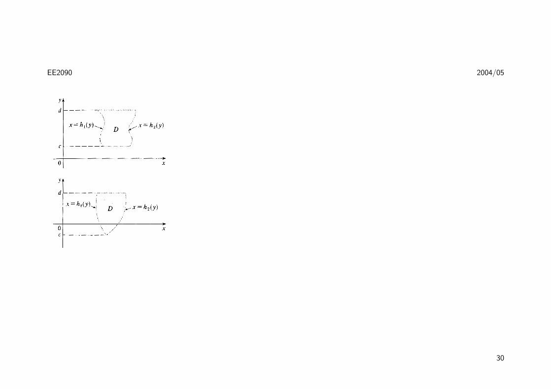
Similarly, we may have
∫ ∫D
f(x, y)dA =
d∫c
∫ h2(y)
h1(y)
f(x, y) dxdy.
D in this case is called a type II region
29
EE2090 2004/05
30
EE2090 2004/05
Examples:
1. Evaluate∫ ∫
D
(x + 2y) dA, where D is the region bounded by the
parabolas y = 2x2 and y = 1 + x2.
Solution:
We need first to determine the boundaries of the region D. In
this respect, it is always helpful to draw a sketch.
31

EE2090 2004/05
The parabolas intersect when 2x2 = 1 + x2, so that x2 = 1, that
is x = ±1. Referring to the figure, we note that the region is of
type I. The lower boundary is y = 2x2 and the upper boundary is
32

EE2090 2004/05
y = 1 + x2. So
∫ ∫D
(x + 2y) dA =
1∫−1
∫ 1+x2
2x2(x + 2y) dydx
=
1∫−1
[xy + y2
]1+x2
y=2x2 dx
=
1∫−1
(−3x4 − x3 + 2x2 + x + 1) dx
33

EE2090 2004/05
= −3x5
5− x4
4+ 2
x3
3+
x2
2+ x
]1
−1
=3215
♦
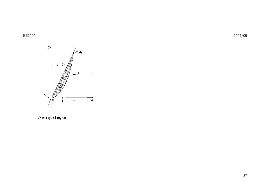
2. Find the volume of the solid that lies under the paraboloid
z = x2 + y2 and above the region D in the xy-plane bounded by
the line y = 2x and the parabola y = x2.
34

EE2090 2004/05
Solution:
Figures show that it is possible to take the region D as either of
type I or type II! Either case will yield the same result!
Taking D as a type I region yields
V =∫ ∫
D
(x2 + y2) dA =
2∫0
∫ 2x
x2(x2 + y2) dydx
35

EE2090 2004/05
whereas, taking it as type II gives
V =∫ ∫
D
(x2 + y2) dA =
4∫0
∫ √y
12y
(x2 + y2) dxdy
and either should yield an answer of 21635 . ♦
36
EE2090 2004/05
37

EE2090 2004/05
38

EE2090 2004/05
3. Evaluate∫ ∫
Dxy dA, where D is the region bounded by the line
y = x− 1 and the parabola y2 = 2x + 6.
Solution:
From the sketches,again D is both type I and type II.
39

EE2090 2004/05
However, it is more complicated to deal with it as a type I region
because the lower boundary consists of two parts! It is therefore
preferable to express D as a type II region, giving the double
40

EE2090 2004/05
integral as :∫ ∫D
xy dA =∫ 4
−2
∫ y+1
12y2−3
xy dxdy =∫ 4
−2
[x2
2y
]x=y+1
x=12y2−3
dy
=12
∫ 4
−2
(−y5
4+ 4y3 + 2y2 − 8y
)dy
=12
[−y6
24+ y4 + 2
y3
3− 4y2
]4
−2
= 36
♦
41
EE2090 2004/05
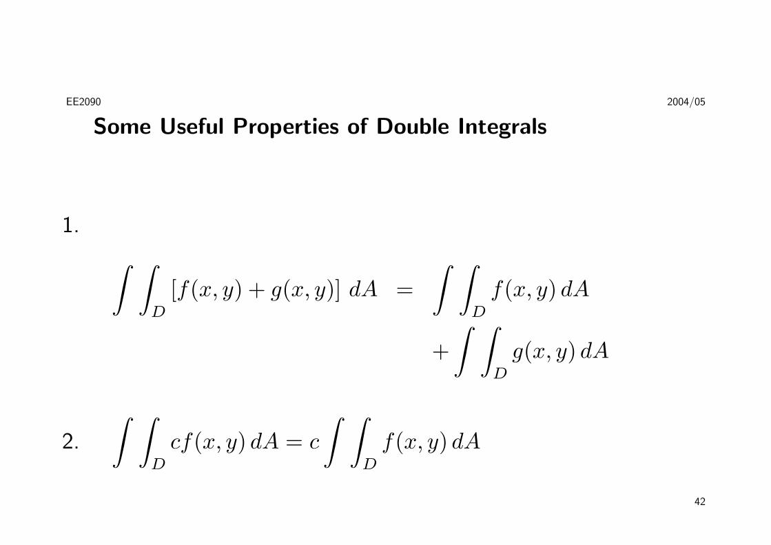
Some Useful Properties of Double Integrals
1. ∫ ∫D
[f(x, y) + g(x, y)] dA =∫ ∫
D
f(x, y) dA
+∫ ∫
D
g(x, y) dA
2.
∫ ∫D
cf(x, y) dA = c
∫ ∫D
f(x, y) dA
42

EE2090 2004/05
3. ∫ ∫D
f(x, y) dA =∫ ∫
D1
f(x, y) dA
+∫ ∫
D2
f(x, y) dA
4. Putting f(x, y) = 1 and integrate over a region D, we get the
area of D:∫ ∫D
dA = A(D)
43
EE2090 2004/05
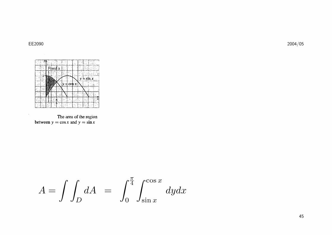
Example:
Find the area of the region D between y = cos x and y = sin x
over the interval 0 ≤ x ≤ π4
Solution:
From the graph, we find that
44
EE2090 2004/05
A =∫ ∫
D
dA =∫ π
4
0
∫ cos x
sin x
dydx
45

EE2090 2004/05
=∫ π
4
0
y]y=cos xy=sin x dx
=∫ π
4
0
[cos x− sinx] =√
2− 1
♦
46

EE2090 2004/05
Double Integrals in Polar Coordinates
• Description of the region of integration, R may be rather
complicated in terms of rectangular coordinates;
• A change of coordinate system may greatly simply the problem;
• One such case is as shown in the figure and a change to polar
coordinates greatly simplifies the problem.
47
EE2090 2004/05
• Recall that the polar coordinates (r, θ) of a point are related to
the rectangular coordinates (x, y) by
r2 = x2 + y2 x = r cos θ y = r sin θ
48
EE2090 2004/05
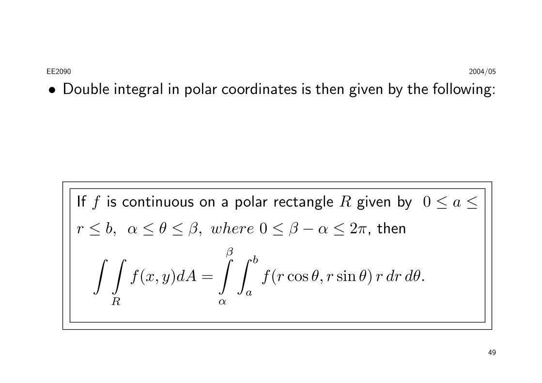
• Double integral in polar coordinates is then given by the following:
If f is continuous on a polar rectangle R given by 0 ≤ a ≤r ≤ b, α ≤ θ ≤ β, where 0 ≤ β − α ≤ 2π, then∫ ∫
R
f(x, y)dA =
β∫α
∫ b
a
f(r cos θ, r sin θ) r dr dθ.
49

EE2090 2004/05
50

EE2090 2004/05
51

EE2090 2004/05
Examples:
1. Evaluate∫ ∫
R(3x + 4y2) dA where R is the region in the upper
half-plane bounded by the circles x2 + y2 = 1 and x2 + y2 = 4
Solution:
Referring to the figure, the region can be described as
R ={(x, y) | y ≥ 0, 1 ≤ x2 + y2 ≤ 4
}52
EE2090 2004/05
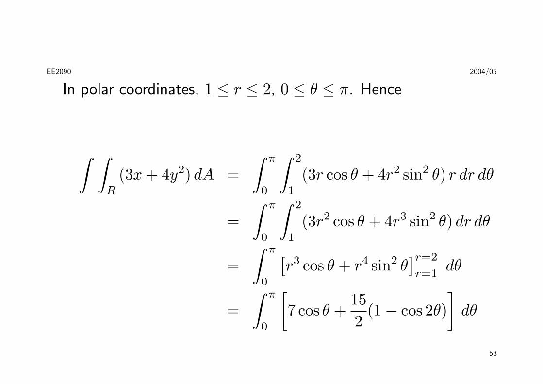
In polar coordinates, 1 ≤ r ≤ 2, 0 ≤ θ ≤ π. Hence
∫ ∫R
(3x + 4y2) dA =∫ π
0
∫ 2
1
(3r cos θ + 4r2 sin2 θ) r dr dθ
=∫ π
0
∫ 2
1
(3r2 cos θ + 4r3 sin2 θ) dr dθ
=∫ π
0
[r3 cos θ + r4 sin2 θ
]r=2
r=1dθ
=∫ π
0
[7 cos θ +
152
(1− cos 2θ)]
dθ
53

EE2090 2004/05
= 7 sin θ +15θ
2− 15
4sin 2θ
]π
0
=15π
2
♦
2. Find the volume of the solid bounded by the plane z = 0 and the
paraboloid z = 1− x2 − y2.
Solution:
Putting z = 0 we get x2 + y2 = 1. So, the plane intersects the
paraboloid in the circle x2 + y2 = 1. The solid thus lies under
the paraboloid and above the circular disk D given by x2+y2 ≤ 1.
54

EE2090 2004/05
55
EE2090 2004/05
In polar coordinate, D is given by 0 ≤ r ≤ 1, 0 ≤ θ ≤ 2π.
Noting that 1− x2 − y2 = 1− r2, the volume is then given by
V =∫ ∫
D
(1− x2 − y2) dA =∫ 2π
0
∫ 1
0
(1− r2) r dr dθ
=∫ 2π
0
dθ
∫ 1
0
(r − r3) dr = 2π
[r2
2− r4
4
]1
0
=π
2
♦
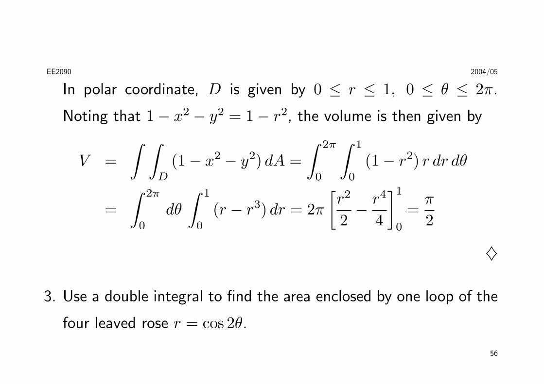
3. Use a double integral to find the area enclosed by one loop of the
four leaved rose r = cos 2θ.
56
EE2090 2004/05
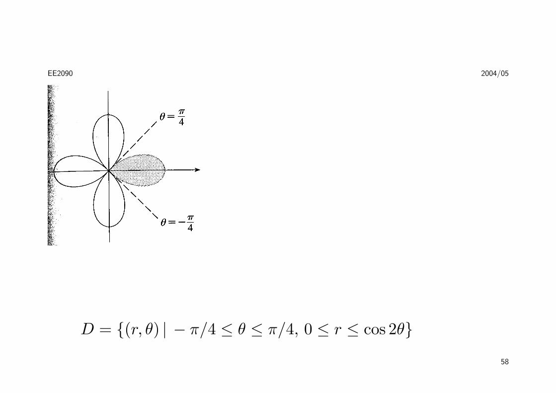
Solution:
From the sketch of the curve, we see that a loop is given by the
region
57
EE2090 2004/05
D = {(r, θ) | − π/4 ≤ θ ≤ π/4, 0 ≤ r ≤ cos 2θ}
58

EE2090 2004/05
So the area is
A(D) =∫ ∫
D
dA =∫ π/4
−π/4
∫ cos 2θ
0
r dr dθ
=∫ π/4
−π/4
[12r2
]cos 2θ
0
dθ =12
∫ π/4
−π/4
cos2 2θ dθ
=14
∫ π/4
−π/4
(1 + cos 4θ) dθ =14
[θ +
14
sin 4θ
]π/4
−π/4
=π
8
♦
59

EE2090 2004/05
We shall now examine the triple integrals
• The Triple Integral of the function f is defined in a similar
manner as that for the double integrals;
• The function f is defined on a rectangular box
B = {(x, y, z) | a ≤ x ≤ b, c ≤ y ≤ d, r ≤ z ≤ s}
• Using the iterated integrals, we can express a triple integral as:
60

EE2090 2004/05
If f is continuous on the rectangular box
B = [a, b]× [c, d]× [r, s], then∫ ∫B
∫f(x, y, z) dV =
∫ s
r
∫ d
c
∫ b
a
f(x, y, z) dx dy dz.
• In the case of a triple integral over a general bounded region E,
we have
61

EE2090 2004/05
E = {(x, y, z) | a ≤ x ≤ b, g1(x) ≤ y ≤ g2(x),
u1(x, y) ≤ z ≤ u2(x, y)}
then∫ ∫E
∫f(x, y, z) dV =
∫ s
r
∫ d
c
∫ b
a
f(x, y, z) dx dy dz.
• Just as in the case of the double integral, setting f(x, y, z) = 1
62

EE2090 2004/05
for all points in E, the triple integral represents the volume of E:
V (E) =∫ ∫
E
∫dV
63

EE2090 2004/05
Examples:
1. Evaluate the triple integral∫ ∫
B
∫xyz2 dV , where B is the
rectangular box given by
B = {(x, y, z) | 0 ≤ x ≤ 1, −1 ≤ y ≤ 2, 0 ≤ z ≤ 3}
Solution:∫ ∫B
∫xyz2 dV =
∫ 3
0
∫ 2
−1
∫ 1
0
xyz2 dx dy dz
64

EE2090 2004/05
=∫ 3
0
∫ 2
−1
[x2yz2
2
]x=1
x=0
dy dz
=∫ 3
0
[y2z2
4
]y=2
y=−1
dz =z3
4
]3
0
=274
♦note that the order of integration does not matter
65
EE2090 2004/05
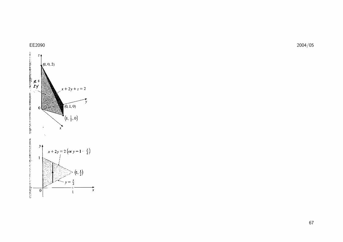
2. Use triple integral to find the volume of the tetrahedron T
bounded by the planes x + 2y + z = 2, x = 2y, x = 0, and
z = 0.
Solution:
The tetrahedron T and its projection D on the xy-plane are
shown in figures.
66
EE2090 2004/05
67

EE2090 2004/05
The lower boundary of T is the plane z = 0 and the upper
boundary is the plane x + 2y + z = 2, that is, z = 2 − x − 2y.
Therefore:
V (T ) =∫ ∫
T
∫dV =
∫ 1
0
∫ 1−x/2
x/2
∫ 2−x−2y
0
dz dy dx
=∫ 1
0
∫ 1−x/2
x/2
(2− x− 2y) dy dx =13
♦
68
EE2090 2004/05
SEQUENCES
A sequence is a succession of numbers that are listed according
to a given prescription or rule. We can write the sequence explicitly
as:
a1, a2, . . . , an, . . .
where n is a positive integer,
or simply as {an}
For example 1, 12,
13, · · · ,
1n, · · · is a sequence and an = 1
n.
69
EE2090 2004/05
• an is called the general term
• an+1 is the successor
• an−1 is the predecessor
We can also write out the ”rule” as a general term and generate
the sequence subsequently. For instance:
an = nn+1 generates a1 = 1
2, a2 = 23, a3 = 3
4, · · ·
Formally, we can state:
70

EE2090 2004/05
A sequence {an} is a function whose domain is a set of nonnegative
integers and whose range is a subset of the real numbers.
The functional values a1, a2, a3, . . . are called the terms of
the sequence, and an, is called the nth term, or the general term,
of the sequence.
71
EE2090 2004/05
LIMITS OF SEQUENCES
How does a given sequence {an} behave as n gets arbitrarily
large ?
Consider the sequence whose an = nn+1
This generates:
a1 =12, a2 =
23, a3 =
34, · · ·
It appears that the terms of the sequence are approaching 1 as n
increases!!
72
EE2090 2004/05
In general, if the terms of the sequence approach the number L
as n increases without bound, we say that the sequence converges
to the limit L and write
L = limn→∞
an
In the above example we would expect
L = limn→∞
n
n + 1= 1
We may define formally the above results as follows:
73

EE2090 2004/05
The sequence {an} converges to the number L, and we write
L = limn→∞
an
if for every ε > 0, there is an integer N such that
|an − L| < ε
whenever n > N . Otherwise, the sequence diverges.
Note that the notation L = limn→∞
an means that eventually the
terms of the sequence {an}, can be made as close to L as may be
desired by taking n sufficiently large.
74

EE2090 2004/05
The following results should be useful:
Theorem 1. [Limit theorem for sequences]
If limn→∞
an = L and limn→∞
bn = M , then
Linearity rule for sequences
limn→∞
(ran + sbn) = rL + sM
Product rule for sequences
limn→∞
(anbn) = LM
75

EE2090 2004/05
Quotient rule for sequences
limn→∞
anbn
= LM provided M 6= 0
Root rule for sequences
limn→∞
m√
an = m√
L provided m√
an is defined for all n and m√
L
exists.
76

EE2090 2004/05
Examples of Convergent sequences
Find the limit of each of these convergent sequences:
1.
{100n
}
2.
{2n2 + 5n− 7
n3
}
3.
{3n4 + n− 15n4 + 2n + 1
}
77
EE2090 2004/05
Solutions
1. As n grows arbitrarily large, 100/n gets smaller and smaller.
Thus,
limn→∞
100n
= 0
♦
2. We cannot use the quotient rule of Theorem 1 because neither
78

EE2090 2004/05
the limit in the numerator nor the one in the denominator exists.
However,
2n2 + 5n− 7n3
=2n
+5n2− 7
n3
and by using the linearity rule, we then have
limx→∞
2n2 + 5n− 7n3
= limn→∞
2n
+ 5 limn→∞
1n2
−7 limn→∞
1n3
= 0 + 0 + 0
79
EE2090 2004/05
= 0 ♦
3. Divide the numerator and denominator by n4 , the highest power
of n that occurs in the expression, to obtain
limn→∞
3n4 + n− 15n4 + 2n2 + 1
= limn→∞
3 + 1n3 − 1
n4
5 + 2n2 + 1
n4
=35
♦
80

EE2090 2004/05
Examples of Divergent sequences
Show that the following sequences diverge:
1. {(−1)n}
2.
{n5 + n3 + 27n4 + n2 + 3
}
Solution:
1. The sequence defined by {(−1)n} is −1, 1, −1, 1, . . . and this
81
EE2090 2004/05
sequence diverges by oscillation because the nth term is always
either 1 or −1. Thus an cannot approach one specific number L
as n grows large. ♦
2. limn→∞
n5 + n3 + 27n4 + n2 + 3
= limn→∞
1 + 1n2 + 2
n5
7n + 1
n3 + 3n5
The numerator tends toward 1 as n → ∞, and the denominator
approaches 0. Hence the quotient increases without bound, and
the sequence must diverge. ♦
The following theorem relates how the limit of a sequence can be
82

EE2090 2004/05
deduced from the limit of a continuous function:
Theorem 2. Given the sequence {an}, let f be a continuous
function such that an = f(n) for n = 1, 2, . . .. If limx→∞
f(x) exists
and limx→∞
f(x) = L, the sequence {an} converges and limn→∞
an = L.
Before proceeding further, the following result is always helpful:
83

EE2090 2004/05
l’Hospital’s Rule
Let f and g be differentiable functions with g′(x) 6= 0
on an open interval containing c (except possibly at c
itself). Suppose
limx→∞
f(x)g(x)
produces an indeterminate form 00 or ∞
∞ and that
limx→∞
f ′(x)g′(x) = L where L is either a finite number,
+∞, or −∞. Then
limx→∞
f(x)g(x)
= L
84
EE2090 2004/05
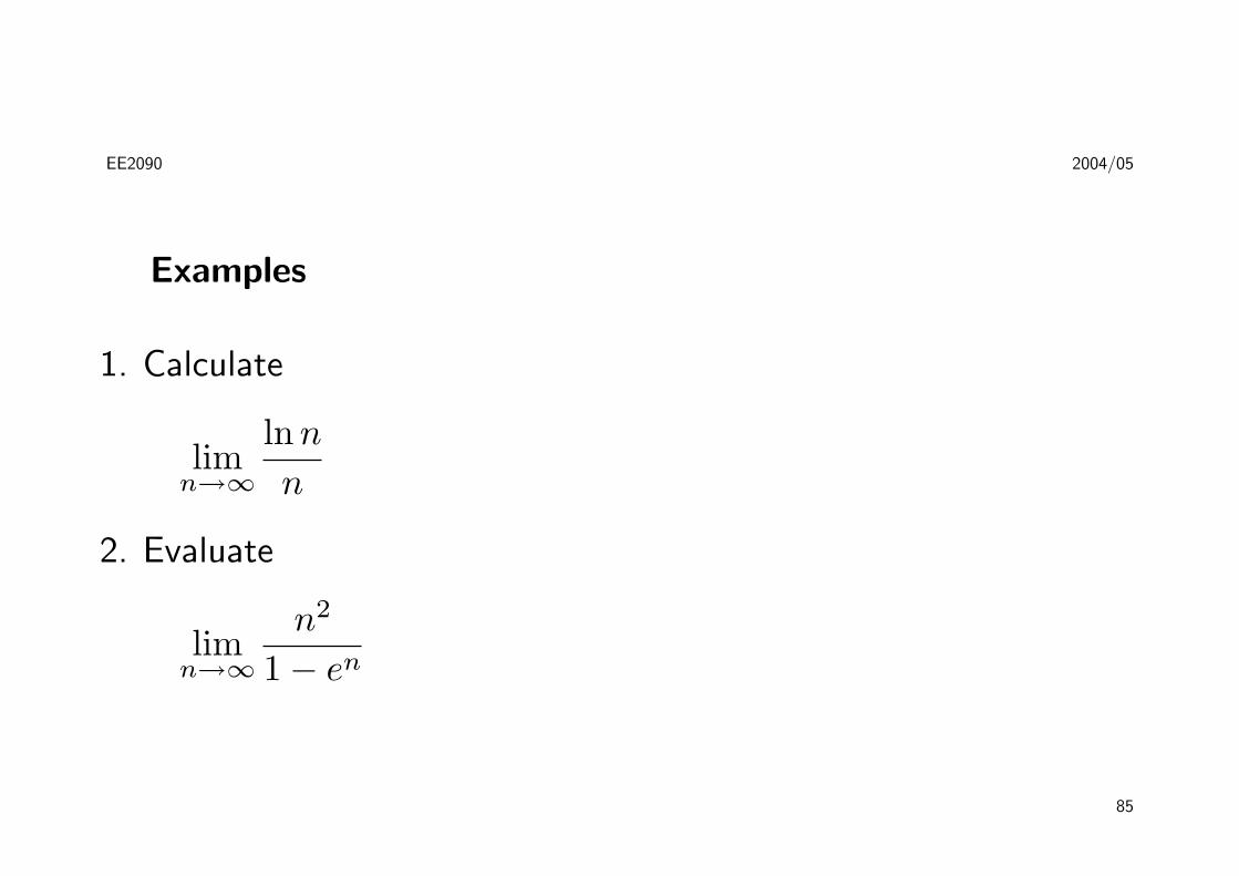
Examples
1. Calculate
limn→∞
lnn
n
2. Evaluate
limn→∞
n2
1− en
85

EE2090 2004/05
Solution
1. Note that both numerator and denominator approach ∞ as
n → ∞. Also note that l’Hospital’s Rule cannot be applied
directly to sequences but to functions of real variables.
So, we should first apply the Rule to related function
f(x) = lnx/x
86

EE2090 2004/05
and obtain
limx→∞
lnx
x= lim
x→∞
1/x
1= 0
By Theorem 2, we have
limn→∞
lnn
n= 0
♦
87

EE2090 2004/05
2. By a similar approach, we have
limx→∞
x2
1− ex= lim
x→∞
2x
−ex
= limx→∞
2−ex
= 0
Hence,
limn→∞
n2
1− en= 0
Note that l’Hospital’s Rule is being applied twice! ♦
88
EE2090 2004/05
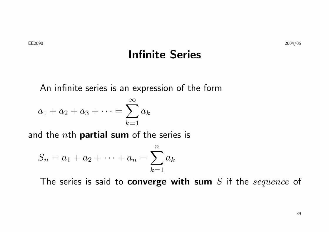
Infinite Series
An infinite series is an expression of the form
a1 + a2 + a3 + · · · =∞∑
k=1
ak
and the nth partial sum of the series is
Sn = a1 + a2 + · · ·+ an =n∑
k=1
ak
The series is said to converge with sum S if the sequence of
89
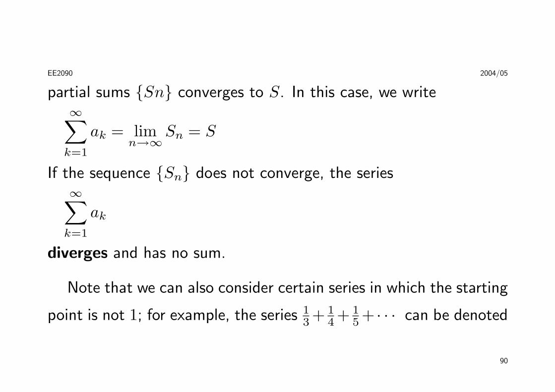
EE2090 2004/05
partial sums {Sn} converges to S. In this case, we write∞∑
k=1
ak = limn→∞
Sn = S
If the sequence {Sn} does not converge, the series∞∑
k=1
ak
diverges and has no sum.
Note that we can also consider certain series in which the starting
point is not 1; for example, the series 13 + 1
4 + 15 + · · · can be denoted
90

EE2090 2004/05
by∞∑
k=3
1k or
∞∑k=2
1k+1
Some Examples
1. Show that the series∞∑
k=1
12k converges.
Solution
This series has the following partial sums:
S1 =12
= 1− 121
91

EE2090 2004/05
S2 =12
+14
= 1− 122
=34
S3 =12
+14
+18
= 1− 123
=78
...
Sn =12
+14
+ · · ·+ 12n
The sequence of partial sums is 12,
34,
78,
1516,
3132,
6364, · · · and in general
92

EE2090 2004/05
(by mathematical induction)
Sn = 1− 12n
Because limn→∞
(1− 12n) = 1, we conclude that the series converges
and its sum is S = 1 ♦
2. Show that the series∞∑
k=1
(−1)k diverges.
Solution
93

EE2090 2004/05
The series can be expanded (written out) as
∞∑k=1
(−1)k = −1 + 1− 1 + 1− 1 · · ·
and we see that the nth partial sum is
Sn =
−1 if n is odd
0 if n is even
Because the sequence {Sn} has no limit, the given series must
diverge. ♦
94
EE2090 2004/05
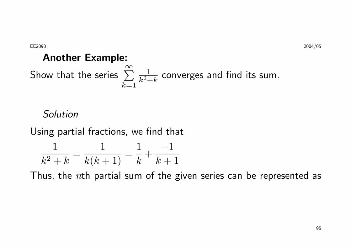
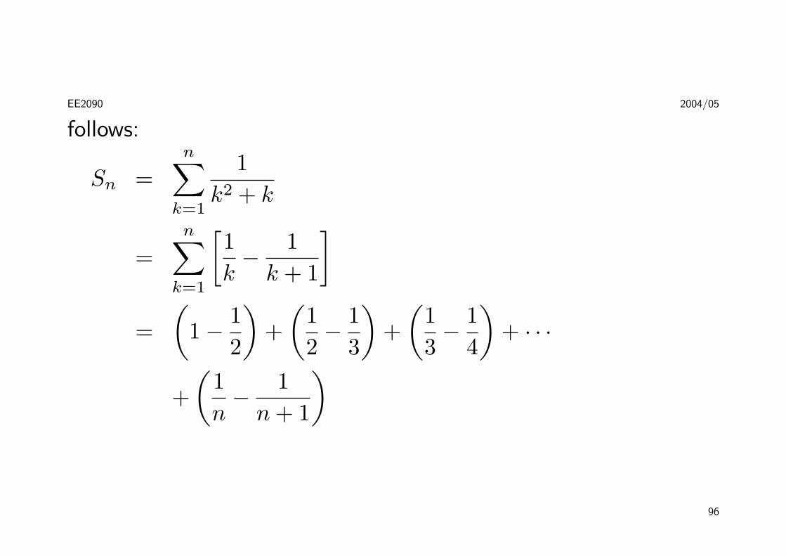
Another Example:
Show that the series∞∑
k=1
1k2+k
converges and find its sum.
Solution
Using partial fractions, we find that
1k2 + k
=1
k(k + 1)=
1k
+−1
k + 1Thus, the nth partial sum of the given series can be represented as
95
EE2090 2004/05
follows:
Sn =n∑
k=1
1k2 + k
=n∑
k=1
[1k− 1
k + 1
]=
(1− 1
2
)+
(12− 1
3
)+
(13− 1
4
)+ · · ·
+(
1n− 1
n + 1
)
96

EE2090 2004/05
= 1 +(−1
2+
12
)+
(−1
3+
13
)+ · · ·
+(−1
n+
1n
)− 1
n + 1
= 1− 1n + 1
The limit of the sequence of partial sums is
limn→∞
Sn = limn→∞
[1− 1
n + 1
]= 1
so the series converges, with sum S = 1. ♦
97

EE2090 2004/05
The above series is called a telescoping series or ( collapsing
series) as there is internal cancellation in the partial sum!
A little note:
When the starting point of a series is not
important, we may denote the series by
writing∑
ak instead of∞∑
k=1
ak
98

EE2090 2004/05
GENERAL PROPERTIES OF INFINITE SERIES
Theorem 3. [Linearity of infinite series]
If∑
ak and∑
bk are convergent series, then so is∑
(cak + dbk)
for constants c, d, and∑(cak + dbk) = c
∑ak + d
∑bk
99
EE2090 2004/05
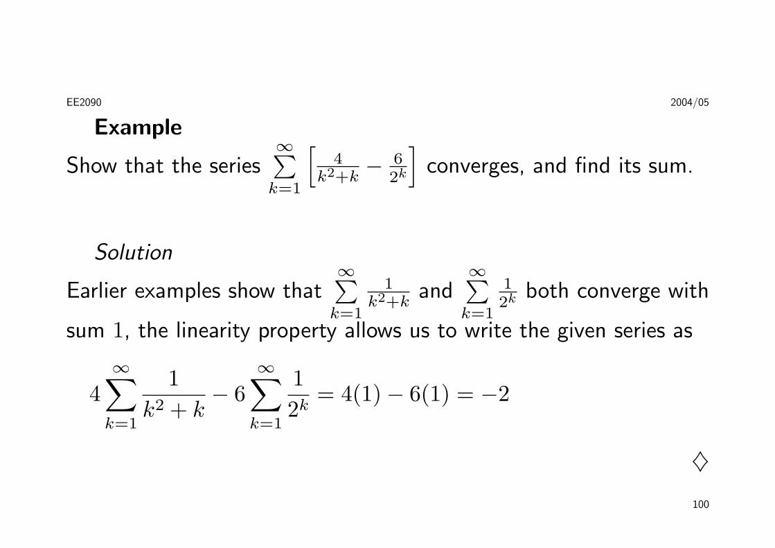
Example
Show that the series∞∑
k=1
[4
k2+k− 6
2k
]converges, and find its sum.
Solution
Earlier examples show that∞∑
k=1
1k2+k
and∞∑
k=1
12k both converge with
sum 1, the linearity property allows us to write the given series as
4∞∑
k=1
1k2 + k
− 6∞∑
k=1
12k
= 4(1)− 6(1) = −2
♦
100
EE2090 2004/05
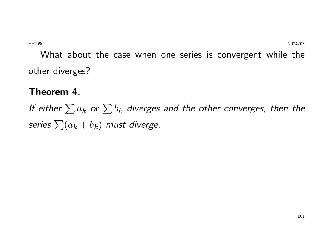
What about the case when one series is convergent while the
other diverges?
Theorem 4.
If either∑
ak or∑
bk diverges and the other converges, then the
series∑
(ak + bk) must diverge.
101
EE2090 2004/05
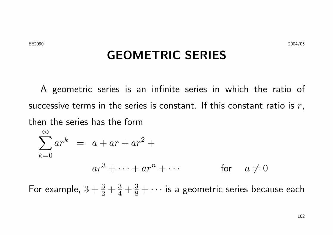
GEOMETRIC SERIES
A geometric series is an infinite series in which the ratio of
successive terms in the series is constant. If this constant ratio is r,
then the series has the form∞∑
k=0
ark = a + ar + ar2 +
ar3 + · · ·+ arn + · · · for a 6= 0
For example, 3 + 32 + 3
4 + 38 + · · · is a geometric series because each
102

EE2090 2004/05
term is 12 the preceding term.
The ratio of a geometric series may be positive or negative. For
example,∞∑
k=0
2(−3)k
= 2− 23
+29− 2
27+ · · ·
is a geometric series with r = −13.
The following theorem tells us how to determine whether a given
geometric series converges or diverges and, if it does converge, what
its sum must be.
103

EE2090 2004/05
Theorem 5. [Geometric series theorem]
The geometric series∞∑
k=0
ark with a 6= 0 diverges if |r| ≥ 1 and
converges if |r| < 1 with sum∞∑
k=0
ark =a
1− r
Example
Determine whether each of the following geometric series converges
or diverges. If the series converges, find its sum.
104

EE2090 2004/05
1.∞∑
k=0
17
(32
)k
2.∞∑
k=2
3(−1
5
)k
Solution
1. r = 32 satisfies |r| ≥ 1, the series diverges. ♦
105

EE2090 2004/05
2. We have r = −15 and |r| < 1, and the geometric series converges.
Note that the first value of k is 2 (not 0), so the value a (the
first value) is a = 3(−15)
2 = 325 and
∞∑k=2
3(−1
5
)k
=a
1− r=
325
1− (−15)
=110
♦
106

EE2090 2004/05
Testing for Convergence or Divergence of a Series
• The convergence or divergence of an infinite series is determined
by the behavior of its nth partial sum, Sn, as n →∞.
• We have used algebraic methods to find formulae for the nth
partial sum of a series.
• It is often difficult or even impossible to find a usable formula
for the nth partial sum of a series, and other techniques must be
107

EE2090 2004/05
used to determine convergence or diverge.
Theorem 6. [The integral test]
If ak = f(k) for k = 1, 2, . . ., where f is a positive, continuous, and
decreasing function of x for x ≥ 1, then∞∑
k=1
ak and
∫ ∞
1
f(x)dx
either both converge or both diverge.
108

EE2090 2004/05
Note the following:
• It is NOT necessary to start the series
or the integral at n = 1.
• It is NOT necessary that f be always
decreasing. What is important is
that f be ultimately decreasing, that
is, decreasing for x larger than some
number!109
EE2090 2004/05
Example - Harmonic series diverges
Test the series (called the harmonic series)∞∑
k=1
1k
= 1 +12
+13
+14
+ · · ·
for convergence.
Solution
Because f(x) = 1x is positive, continuous, and decreasing for x ≥ 1,
110
EE2090 2004/05
the conditions of the integral test are satisfied.∫ ∞
1
1xdx = lim
b→∞
∫ b
1
1xdx = lim
b→∞[ln b− ln 1] = ∞
The integral diverges, so the harmonic series diverges. ♦
Another example
Test the series∞∑
k=1
kek/5 for convergence.
Solution
The function f(x) = xex/5 = xe−x/5 is positive and continuous for
111
EE2090 2004/05
all x > 0. Is it decreasing? We find that
f ′(x) = x
(−1
5e−x/5
)+ e−x/5 =
(1− x
5
)e−x/5
The critical number is found when f ′(x) = 0, so we solve(1− x
5
)e−x/5 = 0
1− x5 = 0
x = 5
We see that f ′(x) < 0 for x > 5, so it follows that f is decreasing for
x > 5. The conditions for the integral test have been established!
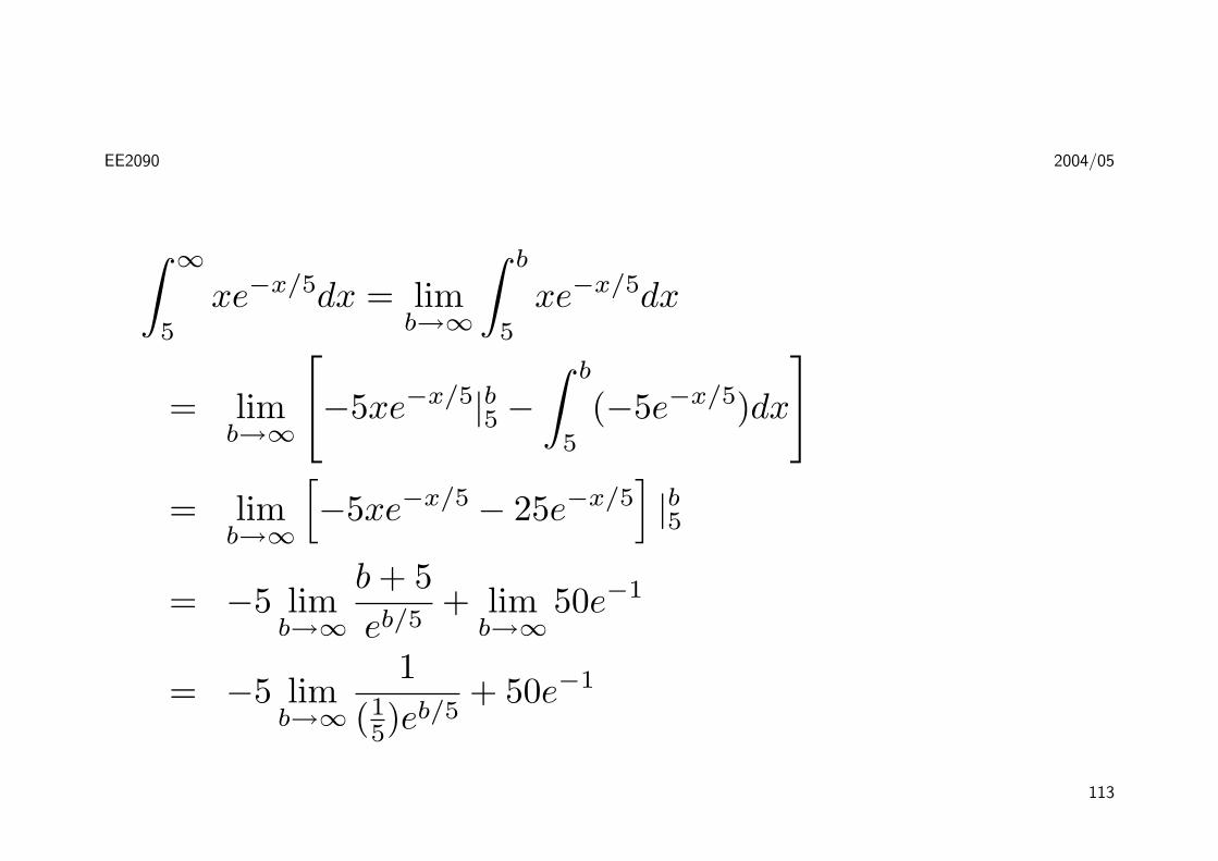
Computing the improper integral, we have:
112
EE2090 2004/05
∫ ∞
5
xe−x/5dx = limb→∞
∫ b
5
xe−x/5dx
= limb→∞
[−5xe−x/5|b5 −
∫ b
5
(−5e−x/5)dx
]= lim
b→∞
[−5xe−x/5 − 25e−x/5
]|b5
= −5 limb→∞
b + 5eb/5
+ limb→∞
50e−1
= −5 limb→∞
1(15)e
b/5+ 50e−1
113

EE2090 2004/05
= 50e−1
Thus, the improper integral converges, which in turn assures the
convergence of given series. ♦
Note, however, that the series converges because the integral
converges to a finite number 50e−1, but this does NOT mean that
the series∞∑
k=1
kek/5 converges to the same number 50e−1!!
114
EE2090 2004/05
Theorem 7. [The Ratio Test]
Given the series∑
ak with ak > 0, suppose that
limk→∞
ak+1
ak= L
The ratio test states the following:
• If L < 1, then∑
ak converges.
• If L > 1 or if L is infinite, then∑
ak diverges.
• If L = 1, the test is in-conclusive.
115
EE2090 2004/05
Example - Convergence using the ratio test
Test the series∞∑
k=1
2k
k! for convergence.
Solution
Let ak = 2k
k! and note that
L = limk→∞
ak+1
ak= lim
k→∞
2k+1
(k+1)!
2k
k!
116

EE2090 2004/05
= limk→∞
k!2k+1
(k + 1)!2k= lim
k→∞
2k + 1
= 0
Thus L < 1, and the ratio test tells us that the given series
converges. ♦
Another example – Divergence using the ratio test
Test the series∞∑
k=1
kk
k! for convergence.
Solution
Let ak = kk
k! and note that
117

EE2090 2004/05
L = limk→∞
ak+1
ak= lim
k→∞
(k+1)k+1
(k+1)!
kk
k!
= limk→∞
k!(k + 1)k+1
kk(k + 1)!= lim
k→∞
(k + 1)k
kk
= limk→∞
(1 +
1k
)k
= e > 1
Because L > 1, the given series diverges. ♦
118

EE2090 2004/05
Theorem 8. [The root test]
Given the series∑
ak with ak ≥ 0, suppose that
limk→∞
k√
ak = L
. The root test states the following:
• If L < 1, then∑
ak converges.
• If L > 1 or if L is infinite, then∑
ak diverges.
• If L = 1, the root test is in-conclusive.
119
EE2090 2004/05
Example - Convergence with the root test
Test the series∞∑
k=2
1(ln k)k for convergence.
Solution
Let ak = 1(ln k)k and note that
L = limk→∞
k√
ak = limk→∞
k
√(ln k)−k
= limk→∞
1ln k
= 0
Because L < 1, the root test tells us that the given series converges.
120
EE2090 2004/05
Another example - Divergence with the root test
Test the series∞∑
k=1
(1 + 1
k
)k2
for convergence.
Solution
L = limk→∞
(1 +
1k
)k21/k
= limk→∞
(1 +
1k
)k
121

EE2090 2004/05
= e > 1
Since L > 1, the series diverges. ♦
Remark
The ratio test is especially useful for series∑
ak for which the
general term ak involves factorials or powers, and the root test
applies naturally if ak involves a power of k.
122

EE2090 2004/05
Vectors in the Plane and in Space
• A vector is a quantity that has both magnitude and direction.
– velocity, force
• A vector is sometimes represented by a directed line, segment,PQ,
with initial point P and terminal point Q. We may write PQ as−−→PQ.
• The magnitude of PQ is denoted as ‖PQ‖
178
EE2090 2004/05
• Two vectors are equal if they have the same magnitude and the
same direction, even if they are in different locations.
• A vector with magnitude 0 is called a null vector or zero vector.
• The 0 vector has no specific direction.
• A scalar multiple sv is parallel to v with magnitude |s|‖v‖ and
points in the same direction as v if s > 0, and in the opposite
direction if s < 0.
179

EE2090 2004/05
• If s = 0 or v = 0, then sv = 0
• Vector addition and subtraction can be realized by the triangle
rule (or the parallelogram rule) and the difference rule.
180

EE2090 2004/05
• Vectors can be conveniently represented using rectangular
coordinates.
– If a vector v is positioned in a rectangular coordinate plane with
its initial point at the origin (0, 0) and its terminal point at
(v1, v2), then v1 and v2 are called the standard components
of v.
– We write v = 〈v1, v2〉
181

EE2090 2004/05
182
EE2090 2004/05
• The following vector properties are important:
〈a1, b1〉= 〈a2, b2〉 if and only if a1 = a2
and b1 = b2
k〈a, b〉= 〈ka, kb〉 for constant k
〈a, b〉+ 〈c, d〉= 〈a + c, b + d〉〈a, b〉 − 〈c, d〉= 〈a− c, b− d〉
• au + bv is called a linear combination of the vectors u and v and
scalar a and b.
183

EE2090 2004/05
– If u = 〈u1, u2〉 and v = 〈v1, v2〉 then
au + bv = a〈u1, u2〉+ b〈v1, v2〉
= 〈au1 + bv1, au2 + bv2〉
Theorem 16. [Properties of Vector Operations]
For any vector u, v, and w in the plane and scalars s and t:
Commutativity of vector addition
u + v = v + u
184
EE2090 2004/05
Associativity of vector addition
(u + v) + w = u + (v + w)
Associativity of scalar multiplication
(st)u = s(tu)
Identity for addition
u + 0 = u
Inverse property for addition
u + (−u) = 0
185
EE2090 2004/05
Distributive laws
(s + t)u = su + tu
s(u + v) = su + sv
Some examples:
1. For the vectors u = 〈2,−3〉 and v = 〈−1, 7〉, find
(a) u + v
(b) 34u
186

EE2090 2004/05
(c) 3u− 12v
Solution:
(a) u + v = 〈2,−3〉+ 〈−1, 7〉 = 〈2 + (−1),−3 + 7〉 = 〈1, 4〉(b) 3
4u = 34〈2,−3〉 = 〈32,
−94 〉
(c) 3u− 12v = 3〈2,−3〉 − 1
2〈−1, 7〉 = 〈132 , −252 〉
♦
2. Show that the line segment joining the midpoints of two sides of
187
EE2090 2004/05
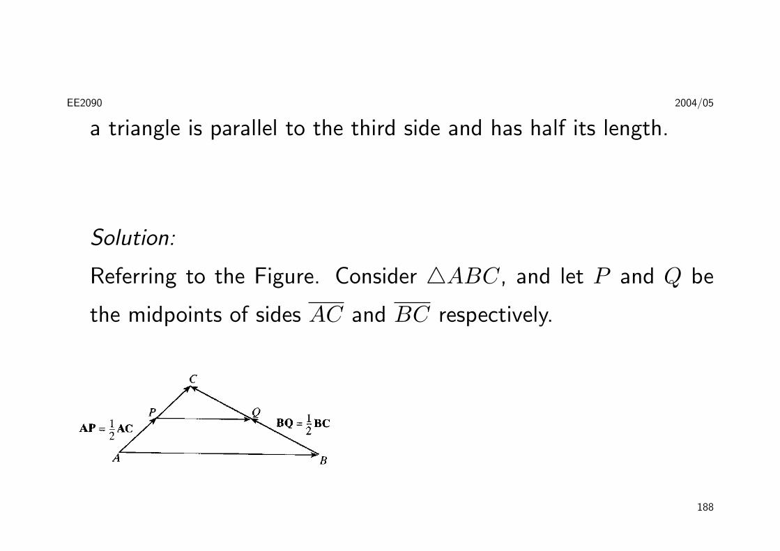
a triangle is parallel to the third side and has half its length.
Solution:
Referring to the Figure. Consider 4ABC, and let P and Q be
the midpoints of sides AC and BC respectively.
188

EE2090 2004/05
We have AP = 12AC and BQ = 1
2BC. Also:
AB = AP + PQ + QB
= 12AC + PQ − BQ
= 12(AB + BC) + PQ − 1
2BC
= 12AB + PQ
12AB = PQ
♦
189
EE2090 2004/05
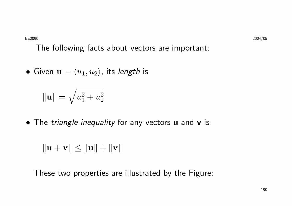
The following facts about vectors are important:
• Given u = 〈u1, u2〉, its length is
‖u‖ =√
u21 + u2
2
• The triangle inequality for any vectors u and v is
‖u + v‖ ≤ ‖u‖+ ‖v‖
These two properties are illustrated by the Figure:
190

EE2090 2004/05
• A unit vector is a vector with length 1
• A direction vector for a given nonzero vector v is a unit vector
191
EE2090 2004/05
u that points in the same direction as v:
u =v‖v‖
• The unit vectors i = 〈1, 0〉 and j = 〈0, 1〉 point in the direction of
the positive x− and y− axes, respectively. They are the standard
basis vectors.
• Any vector v = 〈v1, v2〉 in the plane can be represented as:
v = 〈v1, v2〉 = v1i + v2j
192

EE2090 2004/05
• Extending to 3-dimensional space, we have
v = 〈v1, v2, v3〉 = v1i + v2j + v3k
Some examples:
1. Find a directional vector for v = 〈2,−3〉.Solution:
Noting that ‖v‖ =√
22 + (−3)2 =√
13, we have:
u =v‖v‖
=〈2,−3〉√
13
193

EE2090 2004/05
=1√13〈2,−3〉 =
⟨2√13
,−3√13
⟩
Note that we can also write v = 2i− 3j, then
u =2i− 3j√
13=
2√13
i− 3√13
j
♦
2. If u = 3i + 2j, v = −2i + 5j and w = i − 4j, find the vector
2u + 5v −w.
194

EE2090 2004/05
Solution:
2u + 5v −w = 2(3i + 2j) + 5(−2i + 5j)
−(i− 4j)
= −5i + 33j
♦
3. Two forces, F1 and F2 act on the same body. F1 has a magnitude
of 3 newtons and acts in the direction of −i, whereas F2 has
195

EE2090 2004/05
a magnitude of 2 newtons and acts in the direction of the unit
vector
u =35i− 4
5j
Find the magnitude and direction of the additional force F3 that
must be applied to keep the body at rest.
Solution:
196

EE2090 2004/05
From the given information, we have
F1 = 3(−i) and F2 = 2(35i− 4
5j) =
65i− 8
5j
Let F3 = ai+bj then, for equilibrium, we need F1+F2+F3 = 0.
Thus:
(−3i) + (65i− 8
5j) + (ai + bj) = 0i + 0j
Simplifying, we have
(−3 +65
+ a)i + (−85
+ b)j = 0i + 0j
197

EE2090 2004/05
and thus
−3 + 65 + a = 0 and −8
5 + b = 0
a = 95 b = 8
5
The required force is, F3 = 95i + 8
5j. This is a force of magnitude
‖F3‖ =
√(95)2 + (
85)2 =
15
√145 newtons
which acts in the direction of the unit vector
v =F3
‖F3‖=
5√145
(95i +
85j) =
9√145
i +8√145
j
198
EE2090 2004/05
The Dot Product
The dot product of vectors v = a1i + a2j + a3k and w =
b1i + b2j + b3k is the scalar denoted by v ·wand defined by
v ·w = a1b1 + a2b2 + a3b3
Theorem 17. [Properties of the dot products]
If u, v and w are vectors in <2 or <3 and c is a scalar, then
Magnitude of a vector
199

EE2090 2004/05
v · v = ‖v‖2
Zero product
0 · v = 0
Commutativity
v ·w = w · v
Multiple of a dot product
c(v ·w) = (cv) ·w = v · (cw)
200

EE2090 2004/05
Distributivity
u · (v + w) = u · v + u ·w
An example:
Find the dot product of v = −3i + 2j + k and w = 4i− j + 2k.
Solution:
v ·w = −3(4) + 2(−1) + 1(2) = −12 ♦
201

EE2090 2004/05
Angle between Vectors
• The angle between two vectors plays an important role in certain
applications.
• If θ is the angle between the nonzero vectors v and w, then
cos θ =v ·w‖v‖‖w‖
• Geometrically, we can also use
v ·w = ‖v‖‖w‖ cos θ
202

EE2090 2004/05
• Two vectors are perpendicular or orthogonal, if the angle
between them is θ = π/2
• Nonzero vectors v and w are orthogonal if and only if v ·w = 0
Projections
Let v and w be two vectors in <3 as shown in the Figure.
203
EE2090 2004/05
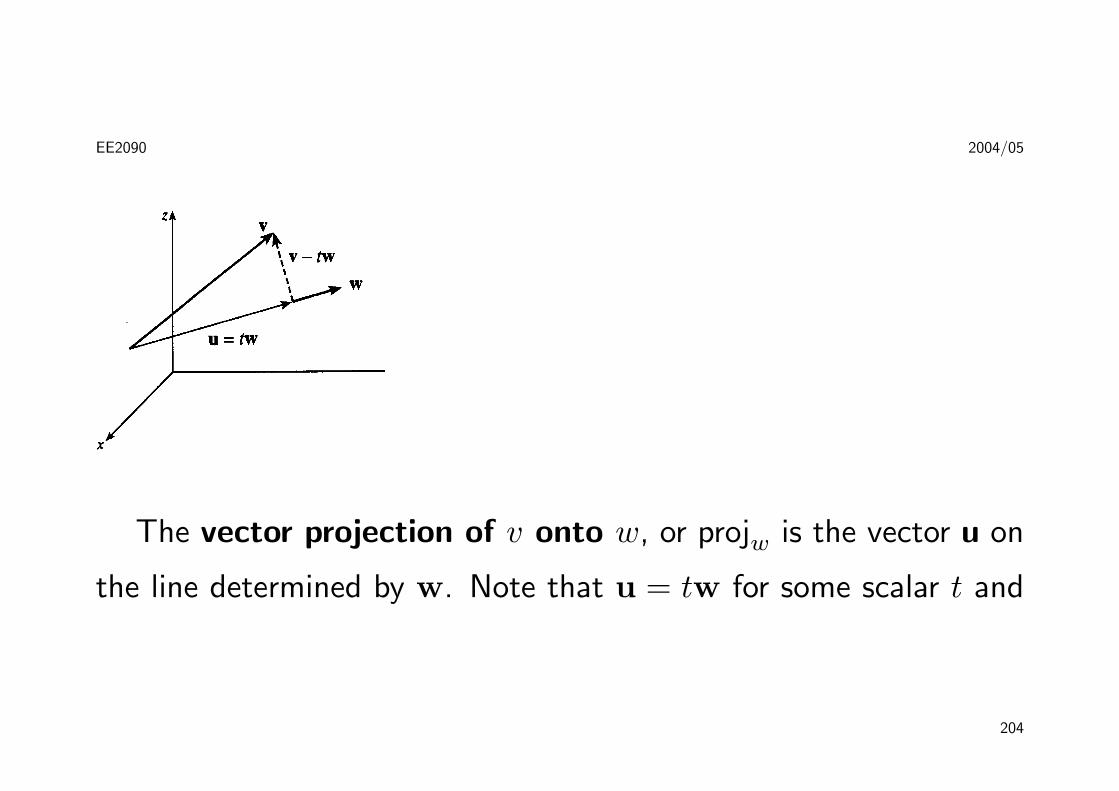
The vector projection of v onto w, or projw is the vector u on
the line determined by w. Note that u = tw for some scalar t and
204

EE2090 2004/05
that v − tw is orthogonal to w. Thus,
(v − tw) ·w = 0
v ·w = t(w ·w)
t = v·ww·w
and the vector projection is
u =(v ·ww ·w
)w
Since w ·w = ‖w‖2, we have
projwv =(
v ·w‖w‖2
)w
205

EE2090 2004/05
=(
v ·w‖w‖
)w‖w‖
The scalar(
v·w‖w‖
)is called the scalar projection of v onto w, or
the component of v in the direction of w, or compwv. Note that
• w‖w‖ is the direction vector for w,
• compwv = v·w‖w‖ = ‖v‖ cos θ, since
(v ·w = ‖v‖‖w‖ cos θ)
206
EE2090 2004/05
.
An example:
Find the vector and scalar projections of v = 2i + 3j + 5k onto
w = 2i− 2j− k.
Solution:
The vector projection of v onto w is
projwv =(v ·ww ·w
)w
207
EE2090 2004/05
=(
2(2) + (3)(−2) + 5(−1)22 + (−2)2 + (−1)2
)(2i− 2j− k)
= −79(2i− 2j− k) = −14
9i +
149
j +79k
compwv =v ·w‖w‖
=2 · 2 + 3 · (−2) + 5 · (−1)√
22 + (−2)2 + (−1)2=−73
♦
Work as a Dot Product
208
EE2090 2004/05
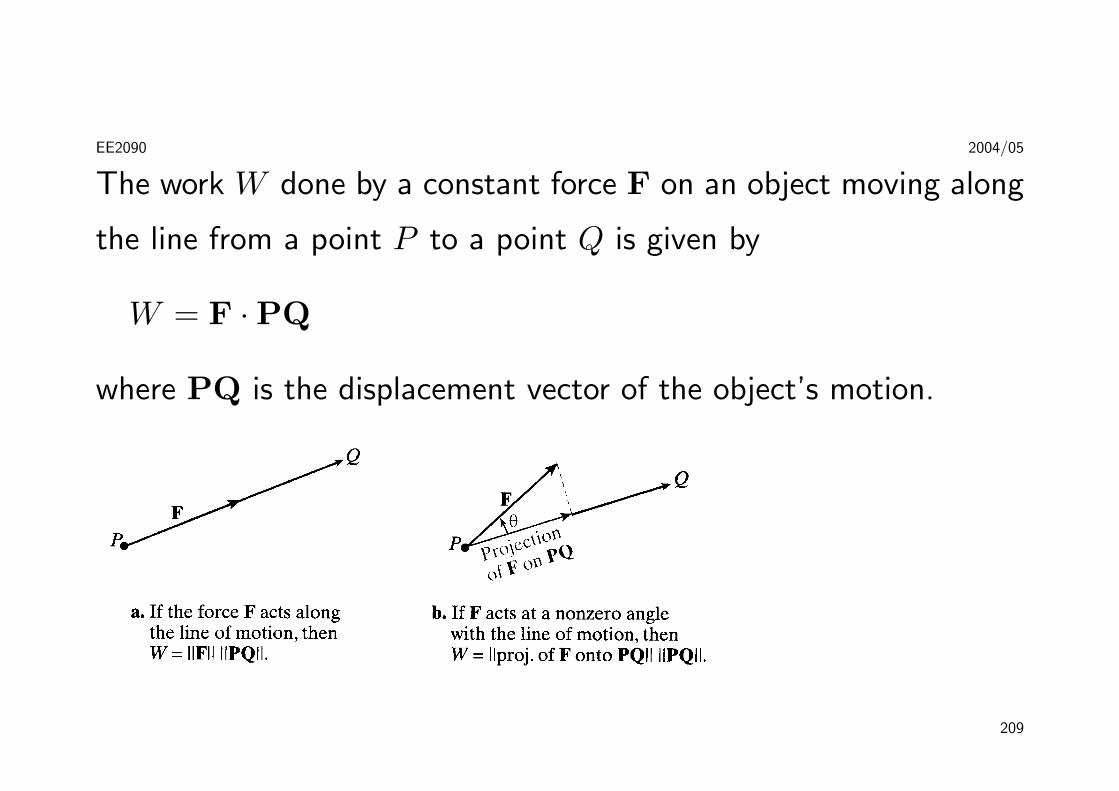
The work W done by a constant force F on an object moving along
the line from a point P to a point Q is given by
W = F ·PQ
where PQ is the displacement vector of the object’s motion.
209

EE2090 2004/05
An example:
A boat sails north aided by a wind blowing in a direction of N30◦E
with magnitude 50 N . How much work is performed by the wind as
the boat moves 10 m?
Solution:
The wind force is ‖F‖ = 50 N , acting in the direction θ = 30◦, as
shown in the Figure. The displacement vector is PQ = 10j. The
210

EE2090 2004/05
force is
F = 50 cos 60◦i + 50 sin 60◦j
The work done is then
W = F ·PQ = 10(25√
3) = 433.01 N −m
211

EE2090 2004/05
♦
212

EE2090 2004/05
The Cross Product
If v = a1i+a2j+a3k and w = b1i+b2j+b3k, the cross product
of the vector v with the vector w, written as v ×w, is the vector
v ×w = (a2b3 − a3b2)i + (a3b1 − a1b3)j + (a1b2 − a2b1)k
A convenient notation for the above is the following determinant
213

EE2090 2004/05
form:
v ×w =
∣∣∣∣∣∣∣∣∣i j k
a1 a2 a3
b1 b2 b3
∣∣∣∣∣∣∣∣∣Expanding the determinant about the first row:
v ×w =
∣∣∣∣∣∣∣∣∣i j k
a1 a2 a3
b1 b2 b3
∣∣∣∣∣∣∣∣∣ =
∣∣∣∣∣∣ a2 a3
b2 b3
∣∣∣∣∣∣ i214
EE2090 2004/05
−
∣∣∣∣∣∣ a1 a3
b1 b3
∣∣∣∣∣∣ j +
∣∣∣∣∣∣ a1 a2
b1 b2
∣∣∣∣∣∣k= (a2b3 − a3b2)i− (a1b3 − a3b1)j
+(a1b2 − a2b1)k
= (a2b3 − a3b2)i + (a3b1 − a1b3)j
+(a1b2 − a2b1)k
215
EE2090 2004/05
Theorem 18. [Properties of the cross product]
If u, w, a, b, and c are vectors in <3 and s and t are scalars, then
Scalar distributivity (sv)× (tw) = st(v ×w)
Distributivity for cross product over addition
u× (v + w) = (u× v) + (u×w)
(u + v)×w = (u×w) + (v ×w)
216

EE2090 2004/05
Anticommutativity
v ×w = −(w × v)
Product of a multiple
v × sv = 0
Zero product
v × 0 = 0× v = 0
217
EE2090 2004/05
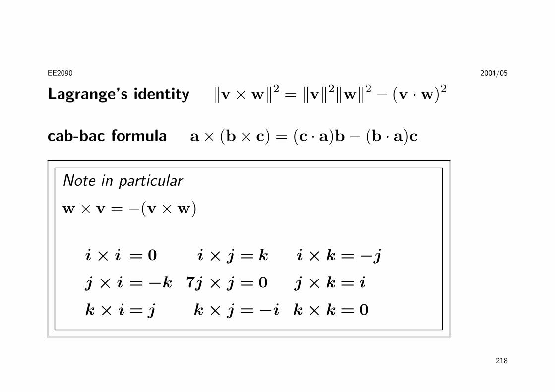
Lagrange’s identity ‖v ×w‖2 = ‖v‖2‖w‖2 − (v ·w)2
cab-bac formula a× (b× c) = (c · a)b− (b · a)c
Note in particular
w × v = −(v ×w)
i × i = 0 i × j = k i × k = −j
j × i = −k 7j × j = 0 j × k = i
k × i = j k × j = −i k × k = 0
218
EE2090 2004/05
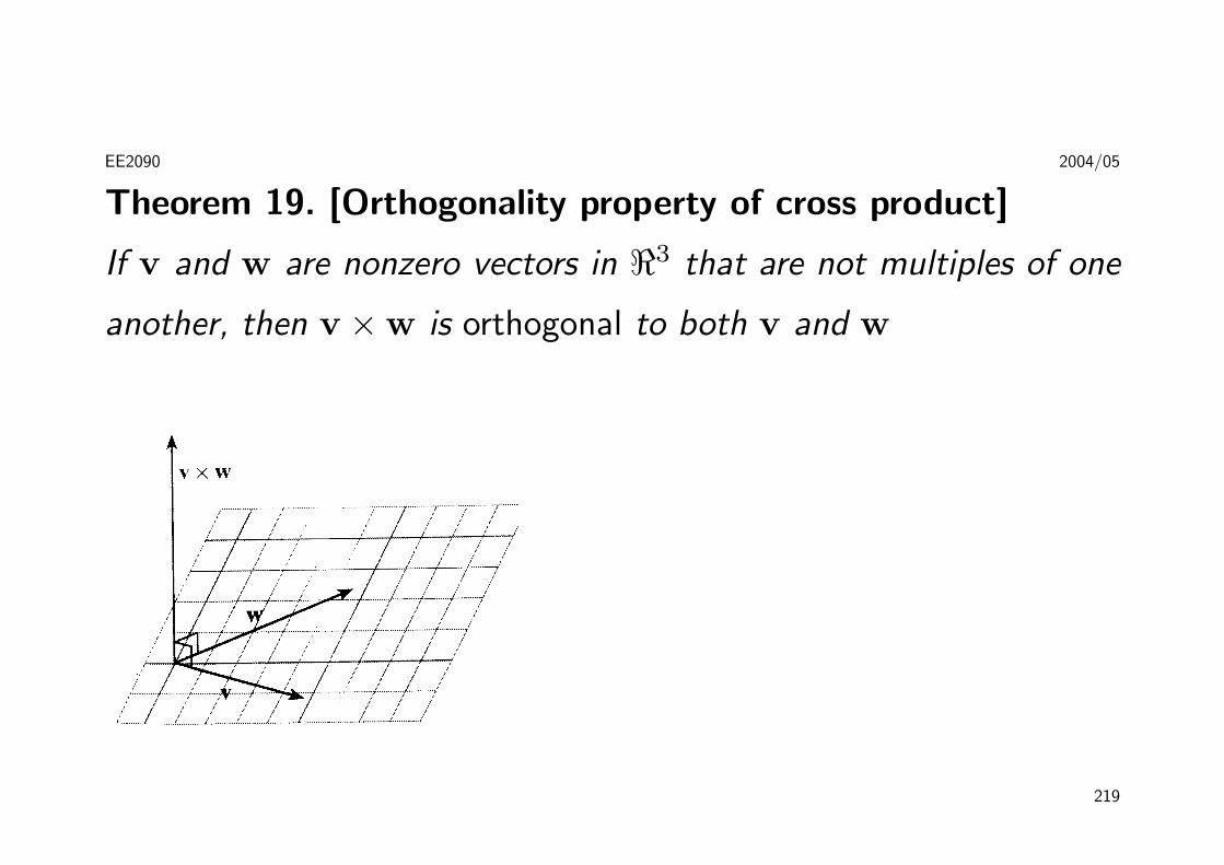
Theorem 19. [Orthogonality property of cross product]
If v and w are nonzero vectors in <3 that are not multiples of one
another, then v ×w is orthogonal to both v and w
219

EE2090 2004/05
The Right-Hand Rule
To determine the direction of the vector (v × w), place the little
finger of the right hand along v and curl the fingers toward w to
cover the smaller angle between v and w, then the thumb points in
the direction of v ×w.
220

EE2090 2004/05
Theorem 20. [Magnitude of the cross product]
If v and w are nonzero vectors in <3 with θ the angle between v
221
EE2090 2004/05
and w (0 ≤ θ ≤ π), then
‖v ×w‖ = ‖v‖‖w‖ sin θ
Applications of cross product: Area and Torque
• Referring to the Figure, let v be defined by AB and w by AC.
Then the parallelogram with adjacent side AB and AC has
AREA = ‖AB×AC‖
222

EE2090 2004/05
The triangle ABC has
AREA =12‖AB×AC‖
223
EE2090 2004/05
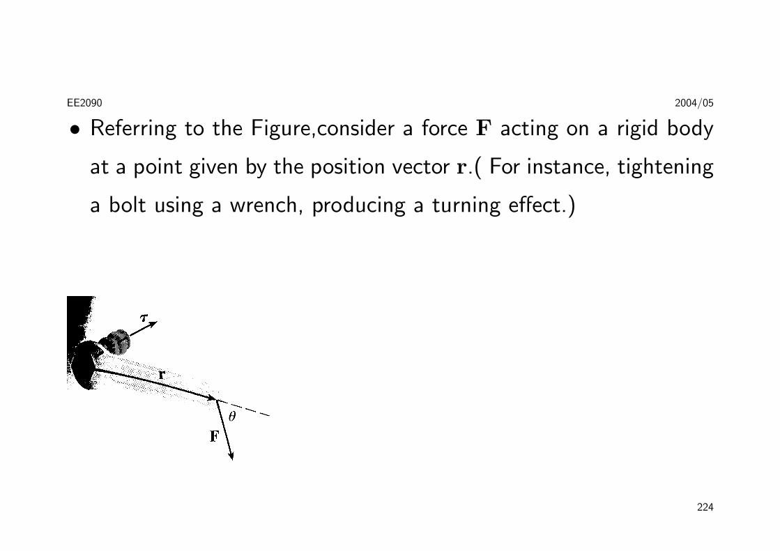
• Referring to the Figure,consider a force F acting on a rigid body
at a point given by the position vector r.( For instance, tightening
a bolt using a wrench, producing a turning effect.)
224

EE2090 2004/05
The torque τ (relative to the origin), is defined as
τ = r × F
and measures the tendency of the body to rotate about the origin.
The direction of the torque vector indicates the axis of rotation.
The magnitude of the torque vector is
|τ | = |r× F| = |r||F| sin θ
where θ is the angle between the position and force vectors. It is
225

EE2090 2004/05
interesting to note that only the component of F perpendicular
to r causes rotation!
Some examples:
1. Find the area of the triangle with vertices P (−2, 4, 5), Q(0, 7,−4),
and R(−1, 5, 0).
Solution:
226

EE2090 2004/05
The area of the triangle PQR has area
A =12‖PQ×PR‖
First find:
PQ = (0 + 2)i + (7− 4)j + (−4− 5)k = 2i + 3j− 9k
PR = i + j− 5k
227
EE2090 2004/05
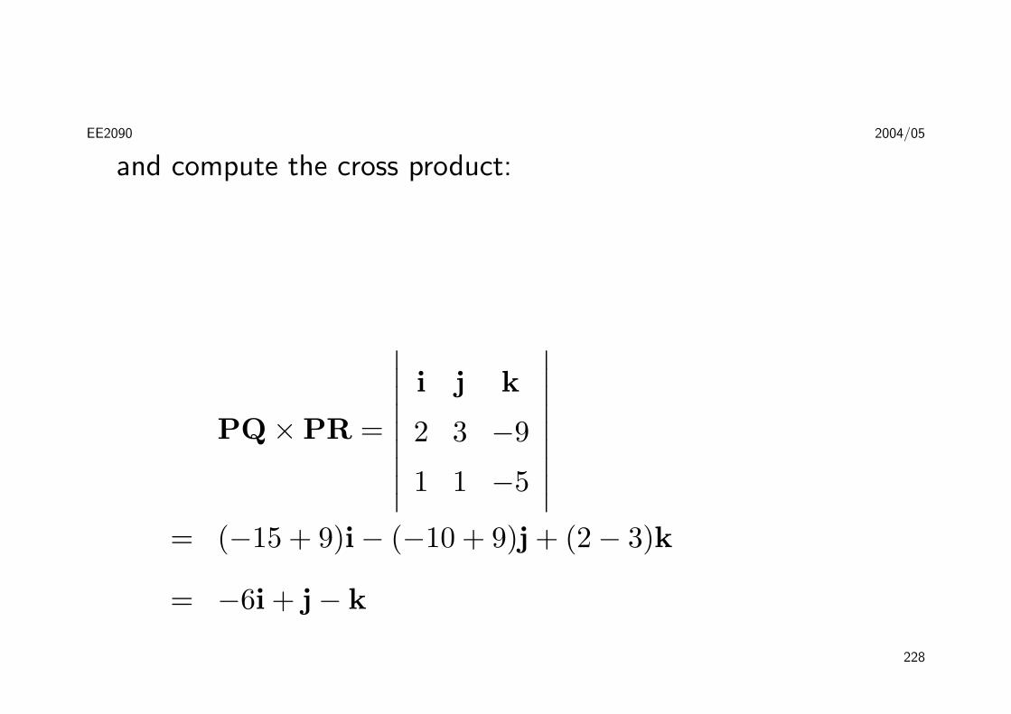
and compute the cross product:
PQ×PR =
∣∣∣∣∣∣∣∣∣i j k
2 3 −9
1 1 −5
∣∣∣∣∣∣∣∣∣= (−15 + 9)i− (−10 + 9)j + (2− 3)k
= −6i + j− k
228

EE2090 2004/05
Thus the area is
A =12‖PQ×PR‖
=12
√(−6)2 + 12 + (−1)2 =
12
√38
♦
2. The figure shows a half open door that is 3 ft wide. A force of
30 lb is applied in a horizontal direction at the edge of the door.
229

EE2090 2004/05
Find the torque of the force about the hinges on the door.
Solution:
Using the coordinate system assigned, F = −30i. The door is
230

EE2090 2004/05
half open, it makes an angle of π4 as shown. The ”position” vector
PQ is represented by
PQ = 3(cosπ
4i + sin
π
4j)
=3√
22
i +3√
22
j
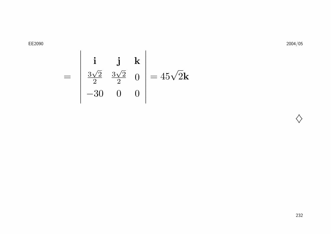
The torque can thus be found:
T = PQ× F
231
EE2090 2004/05
=
∣∣∣∣∣∣∣∣∣i j k
3√
22
3√
22 0
−30 0 0
∣∣∣∣∣∣∣∣∣ = 45√
2k
♦
232

EE2090 2004/05
Lines and Planes in <3
Parametric Equations -
Parametric Representation for a Curve in <2
Let f and g be continuous functions of t on an interval I; then the
equations
x = f(t) and y = g(t)
are called parametric equations with parameter t. As t varies
233

EE2090 2004/05
over the parametric set I, the points (x, y) = (f(t), g(t)) trace
out a parametric curve.
Examples:
1. Sketch the path of the curve x = t2−9, y = 13t for −3 ≤ t ≤ 2.
Solution:
see the Figure.
234

EE2090 2004/05
♦
235

EE2090 2004/05
2. Describe the path x = sinπt, y = cos 2πt, for 0 ≤ t ≤ 0.5.
Solution:
Using a double angle identity, we have
cos 2πt = 1− 2 sin2 πt
so that
y = 1− 2x2
236
EE2090 2004/05
This is an equation for a parabola. Because t is restricted to an
interval, the parametric representation involves only part of the
right side of the parabola.
237

EE2090 2004/05
♦
238

EE2090 2004/05
Parametric Form of a Line in <3
If L is a line that contains the point (x0, y0, z0) and is parallel to
the vector v = Ai + Bj + Ck, then L has parametric form
x = x0 + tA y = y0 + tB z = z0 + tC
The quantities A,B, C are called the direction numbers, or in
notation [A,B, C]. The vector v is called a direction vector of the
line L.(See Figure)
239

EE2090 2004/05
An Example:
Find parametric equations for the line that contains the point
(3, 1, 4) and is parallel to the vector v = −i + j − 2k. Find where
this line passes through the coordinate planes.
240

EE2090 2004/05
Solution:
The direction numbers are [−1, 1,−2] and x0 = 3, y0 = 1, z0 =
4, so the line has the parametric form
x = 3− t y = 1 + t z = 4− 2t
This line intersects the x− y-plane when z = 0:
0 = 4− 2t implies t = 2
Thus, x = 3 − 2 = 1 and y = 3. This is the point (1, 3, 0).
241

EE2090 2004/05
Similarly, the line intersects the xz-plane at (4, 0, 6) and the yz-
plane at (0, 4,−2).
242

EE2090 2004/05
♦
In the special case where none of the direction numbers A, B or C
is 0, we can obtain the following symmetric equations for a line:
Symmetric Form of a Line in <3:
If L is a line that contains the point (x0, y0, z0) and is parallel to
the vector v = Ai + Bj + Ck, (A, B, C nonzero numbers), then
243
EE2090 2004/05
the point (x, y, z) is on L if and only if its coordinates satisfy
x− x0
A=
y − y0
B=
z − z0
C
An Example:
Find symmetric equations for the line L through the points
P (−1, 3, 7) and Q(4, 2,−1)
244

EE2090 2004/05
Solution:
The required line passes through P and is parallel to the vector
PQ = (4 + 1)i + (2− 3)j + (−1− 7)k = 5i− j− 8k
Thus, the direction numbers are [5,−1,−8]. Choosing P as
(x0, y0, z0), we obtain
x + 15
=y − 3−1
=z − 7−8
♦
245
EE2090 2004/05
Equation of a Plane in <3
• Planes in space can be characterized by vector methods,
• Any plane is completely determined by any one of its points and
its orientation, i.e. the ”direction” it faces,
• The direction of a plane is specify by a vector N that is orthogonal
to every vector in the plane – the normal to the plane.
246

EE2090 2004/05
Example:
Find an equation for the plane that contains the point Q(3,−7, 2)
and is normal to the vector N = 2i + j− 3k.
Solution:
The normal vector V is orthogonal to every vector in the plane. If
point P (x, y, z) is in the plane, then N must be orthogonal to the
vector
QP = (x− 3)i + (y + 7)j + (z − 2)z
247

EE2090 2004/05
Hence
N ·QP = 2(x− 3) + (1)(y + 7) + (−3)(z − 2) = 0
2x− 6 + y + 7− 3z + 6 = 0
2x + y − 3z + 7 = 0
Therefore, 2x + y − 3z + 7 = 0 is the equation of the plane. ♦
Generalizing the approach illustrated in the above example, we
take note of the following:
248

EE2090 2004/05
• The plane that contains the point (x0, y0, z0) and having a normal
vector N = Ai + Bj + Ck must have the equation of the plane
as
A(x− x0) + B(y − y0) + C(z − z0) = 0
This is called the point-normal form of the equation of plane;
• By rearranging the terms, we can have the standard form of the
249

EE2090 2004/05
equation of plane as
Ax + By + Cz + D = 0
• The numbers [A, B, C] are the attitude numbers of the plane.
250

EE2090 2004/05
• The attitude numbers of a plane are the same as direction numbers
of a normal vector!
Some Examples:
1. Find the a normal vector to the plane 5x + 7y − 3z = 0
Solution:
251

EE2090 2004/05
A normal to the plane 5x + 7y − 3z = 0 is
N = 5i + 7j− 3k
♦
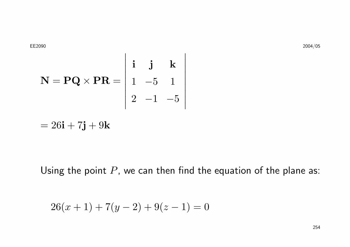
2. Find the standard form equation of a plane containing P (−1, 2, 1),
Q(0,−3, 2), and R(1, 1,−4).
Solution:
252
EE2090 2004/05
The normal N to the required plane is orthogonal to the vectors
PQ and PR, i.e.
N = PR×PQ.
PQ = (0 + 1)i + (−3− 2)j + (2− 1)k = i− 5j + k
PR = (1 + 1)i + (1− 2)j + (−4− 1)k = 2i− j− 5k
253
EE2090 2004/05
N = PQ×PR =
∣∣∣∣∣∣∣∣∣i j k
1 −5 1
2 −1 −5
∣∣∣∣∣∣∣∣∣= 26i + 7j + 9k
Using the point P , we can then find the equation of the plane as:
26(x + 1) + 7(y − 2) + 9(z − 1) = 0
254
EE2090 2004/05
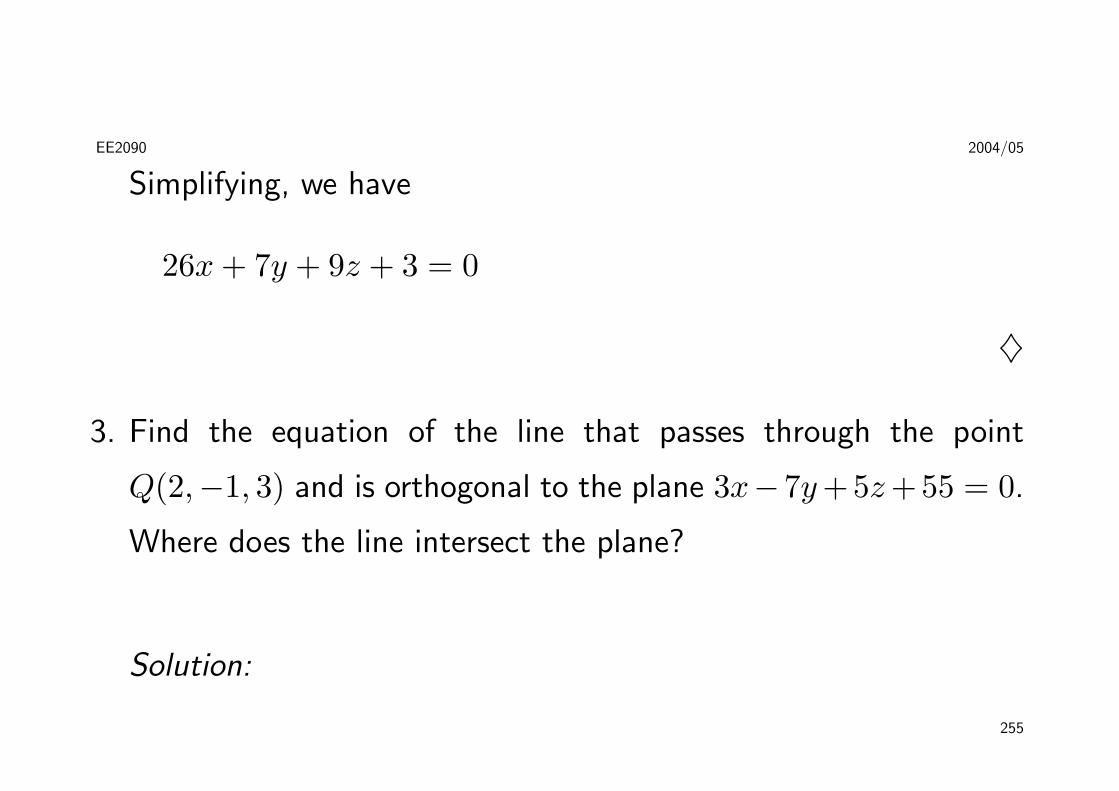
Simplifying, we have
26x + 7y + 9z + 3 = 0
♦
3. Find the equation of the line that passes through the point
Q(2,−1, 3) and is orthogonal to the plane 3x−7y +5z +55 = 0.
Where does the line intersect the plane?
Solution:
255

EE2090 2004/05
By inspection, N = 3i− 7j+5k is a normal vector. The required
line must be parallel to this normal. Thus the line contains the
point Q(2,−1, 3) and has the direction numbers [3,−7, 5], so its
parametric form is
x = 2 + 3t, y = −1− 7t, z = 3 + 5t
Substituting into equation of the plane:
3(2 + 3t)− 7(−1− 7t) + 5(3 + 5t) = −55
256

EE2090 2004/05
t = −1
The point of intersection is found by putting t = −1 into equation
of the line:
x = 2 + 3(−1) = −1
y = −1− 7(−1) = 6
z = 3 + 5(−1) = −2
The point of intersection is (−1, 6,−2) ♦
257

EE2090 2004/05
4. Find the equation of a line passing through (−1, 2, 3) that is
parallel to the line of intersection of the planes 3x − 2y + z = 4
and x + 2y + 3z = 5.
Solution:
By inspection, normals to the planes are N1 = 3i − 2j + k and
N2 = i + 2j + 3k. The desired line is perpendicular to both of
these normals (can you vusualise this?) so a vector parallel to the
258

EE2090 2004/05
line is found by computing the cross product:
N1 ×N2 =
∣∣∣∣∣∣∣∣∣i j k
3 −2 1
1 2 3
∣∣∣∣∣∣∣∣∣= (−6− 2)i− (9− 1)j + (6 + 2)k
= −8(i + j− k)
Thus the required line passes through (−1, 2, 3) and is parallel to
259

EE2090 2004/05
the vector 〈1, 1,−1〉 so it has the parametric form
x = −1 + t, y = 2 + t, z = 3− t
♦
260

EE2090 2004/05
Vector Methods For Measuring Distances in <3
Theorem 21. [Distance from a point to a plane in <3]
The distance from a point P (x0, y0, z0) to the plane Ax + By +
Cz + D = 0 is given by
d =|QP ·N|‖N‖
=|Ax0 + By0 + Cz0 + D|√
A2 + B2 + C2
where Q is any point in the given plane and N is a normal to the
given plane.
261

EE2090 2004/05
Theorem 22. [Distance from a point to a line]
262
EE2090 2004/05
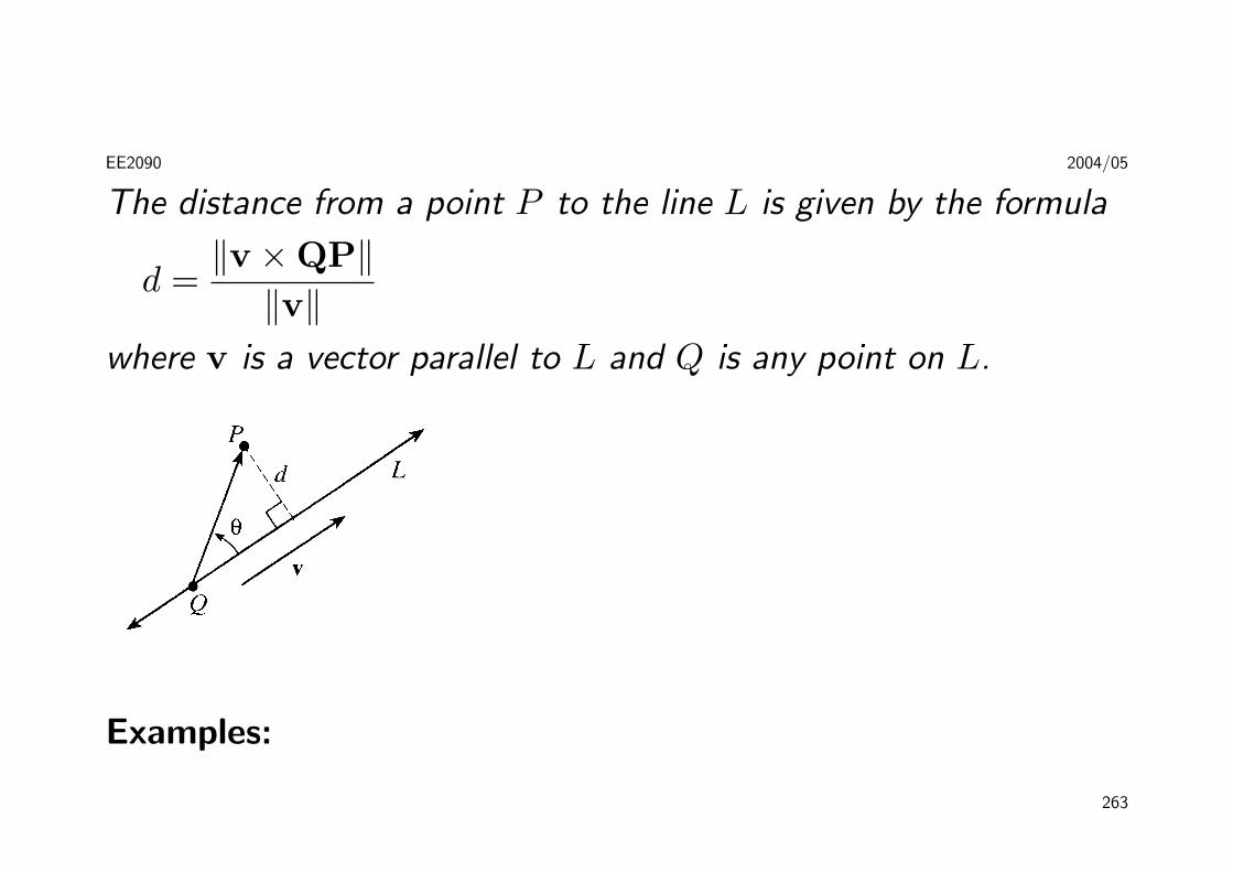
The distance from a point P to the line L is given by the formula
d =‖v ×QP‖
‖v‖where v is a vector parallel to L and Q is any point on L.
Examples:
263
EE2090 2004/05
1. Find an equation for the sphere with center C(−3, 1, 5) that is
tangent to the the plane 6x− 2y + 3z = 9.
Solution:
The radius r of the sphere is the distance from the center C to
264

EE2090 2004/05
the given plane:
r =
∣∣∣∣∣6(−3) + (−2)(1) + 3(5)− 9√62 + (−2)2 + 32
∣∣∣∣∣ =∣∣∣∣−14
7
∣∣∣∣ = 2
The equation of the sphere is
(x + 3)2 + (y − 1)2 + (z − 5)2 = 22
♦
265
EE2090 2004/05
2. Find the distance from the point P (3,−8, 1) to the line
x− 33
=y + 7−1
=z + 2
5
Solution:
We need a point Q on the line. By inspection, Q(3,−7,−2) is
on the line and that QP = 〈0,−1, 3〉. A vector parallel to L is
266

EE2090 2004/05
v = 〈3,−1, 5〉, so that
v ×QP =
∣∣∣∣∣∣∣∣∣i j k
3 −1 5
0 −1 3
∣∣∣∣∣∣∣∣∣= 2i− 9j− 3k
Thus
d =‖v ×QP‖
‖v‖=
√22 + (−9)2 + (−3)2√
32 + (−1)2 + 52≈ 1.64 ♦
267

Introduction
�� Denition
f �t� is a given function with variable t� for all t ��� Laplace Transform �L�T�� of f �t� is
L�f �t�� � F �s� �
Z�
�f �t�e�stdt �����
F �s� is a function of s where s is generally acomplex variable s � � jw�
Original function f �t� is the inverse of F �s�de�ned by
f �t� � L���F �s��
Laplace Transformsslide��

Examples
Example ��
Let f �t� � �� for t � �� Find F �s��
Solution�
L�f �t�� �
Z�
��e�stdt
� �e�st
s
����
��
s
Unit Step Function�
1
t
Laplace Transformsslide��

Examples
The unit step function u�t� is de�ned as follows
u�t� � � � t � �
� � � t � �
Hence
L�u�t�� ��
sSuppose given g�t� only in the interval t � �� we
can rewrite it as g�t�u�t��
X
=
g(t) 1 u(t)
t
g(t)u(t)
t
t
Laplace Transformsslide��

Examples
Example ��
Find the L�T� of f �t� � eat� t � �� where a is aconstant�Solution �
L�f �t�� �
Z�
�eate�stdt
�
Z�
�e��s�a�tdt
� �e��s�a�t
�s� a�
����
��
�s� a�� �s � a� � �
Hence�
F �s� ��
�s � a�for s � a
Laplace Transformsslide��

Examples
Note that from the de�nition of f �t� � eat � t �
�� f �t� can be written as
f �t� � eatu�t�
and
L�eatu�t�� ��
�s� a�� for s � a
Laplace Transformsslide��
Examples
Example ��
Find the L�T� of f �t� � sinh�wt��First note that
sinh�wt� ��
�ewt� e�wt�
Hence
L�sinh�wt�� ��
Z�
�e�te�stdt�
�
Z�
�e��te�stdt
��
��
s� w�
�
s w
�
��
��s w�� �s� w�
s� � w�
��
w
s� � w�
Laplace Transformsslide��

Examples
Example ��
Find the L�T� of f �t� � cosh�wt��First note that
cosh�wt� ��
�ewt e�wt�
Hence
L�cosh�wt�� ��
Z�
�e�te�stdt
�
Z�
�e��te�stdt
��
��
s� w
�
s w
�
��
��s w� �s� w�
s� � w�
��
s
s� � w�
Laplace Transformsslide�

Linearity of Laplace Transforms
�a� Linearity of Laplace Transforms
Theorem ���� The Laplace transformation is
a linear operation� That is for any functions
f �t� and g�t� whose L�T� exist and for any con�
stants a and b
L�af �t� bg�t�� � aL�f �t�� bL�g�t��
Proof�
LHS �
Z�
��af �t� bg�t��e�stdt
� a
Z�
�f �t�e�stdt b
Z�
�g�t�e�stdt
� aL�f �t�� bL�g�t��
Laplace Transformsslide��
Examples
Example �
L�sin�wt�� ��
j
Z�
�ej�te�stdt�
�
j
Z�
�e�j�te�stdt
� L
�ejwt� e�jwt
j
�
��
jL�ejwt� e�jwt�
��
j
��
s� jw�
�
s jw
�
��
j
��s jw�� �s� jw�
s� w�
��
w
s� w�
Laplace Transformsslide���
Examples
Example ��
L�cos�wt�� � L
�ejwt e�jwt
�
��
L�ejwt e�jwt�
��
��
s� jw
�
s jw
�
��
��s jw� �s � jw�
s� w�
��
s
s� w�
Laplace Transformsslide���

Examples
Example ��
L�t� �
Z�
�te�stdt Integrate by parts
Revision� Integration by parts�
Di�erentiation of a product of two functions u�t�and v�t� � from here on simply called u and v�
d
dt�uv� � u
dv
dt v
du
dt
Integrate both sides w�r�t� t and rearrange�
Zudv
dtdt � uv �
Zvdu
dtdt
Laplace Transformsslide���

Examples
Let
L�t� �
Z�
�te�stdt �
Z�
�udv
dtdt
ie� Let u � t and dvdt
� e�st�
L�t� �
�uv �
Zvdu
dtdt
��
�
�
�te�st
�s
��
�
�
Z�
�
�e�st
�s
��dt
� � �
s
�e�st
�s
��
�
��
s�
Laplace Transformsslide���

Examples
Example ��
L�t�� �
Z�
�t�e�stdt
�
Z�
�udv
dtdt
�t�e�st
�s
����
�
s
Z�
� te�stdt
�
s
Z�
�te�stdt
�
s
�
s�
� �
s�
It can be shown by induction that
L�tn� �n�
sn��
Laplace Transformsslide���

Important Laplace Transforms
f �t� F �s� � L�f �t�� �R�
� f �t�e�stdt
� u�t� �s
eat �s�a
� sin�wt� ws��w�
� cos�wt� ss��w�
� sinh�wt� ws��w�
� cosh�wt� ss��w�
� tn n�sn��
Laplace Transformsslide���

Inverse Laplace Transform
�b� Inverse Laplace Transform
The procedure to obtain the inverse Laplace trans�form of F �s� is given in the following steps�
�� First use partial fractions to rewrite thegiven F �s� as a sum of simple terms for whichthe inverse Laplace Transform is straightforward�
� Then take the Inverse L�T� as the sum of theInverse L�T� of the simple terms�
Laplace Transformsslide���

Examples
Example ��Given
F �s� ��
�s� a��s� b�
Find f �t� � L���F �s���
Solution � Use Partial Fractions�
�
�s� a��s� b��
A
s� a
B
s� b
Multiplying both sides by �s� a��s� b�� we have
� � A�s� b� B�s � a�
Let s � a�
� � A�a� b�
or
A ��
�a� b�
Laplace Transformsslide���

Examples
Let s � b�
� � B�b� a�
or
B ��
�b� a�
Hence�
�s� a��s� b��
�
�a� b�
�
�s � a�
�
�b� a�
�
�s� b�
��
�a� b��
�
�s� a��
�
�s� b��
Laplace Transformsslide��
Examples
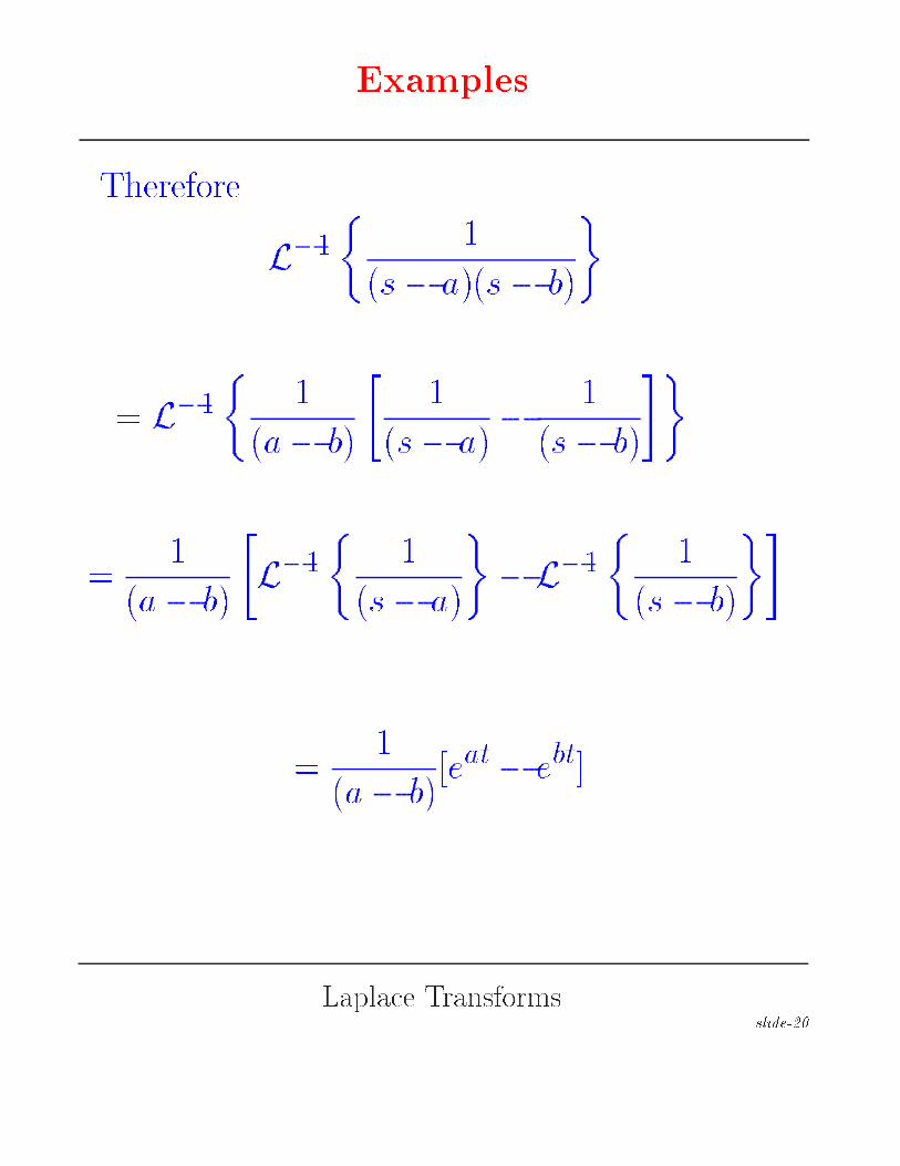
Therefore
L���
�
�s� a��s� b�
�
� L���
�
�a� b�
��
�s � a��
�
�s� b�
��
��
�a� b�
�L��
��
�s� a�
�� L��
��
�s� b�
��
��
�a� b��eat� ebt�
Laplace Transformsslide��
Properties of Laplace Transforms
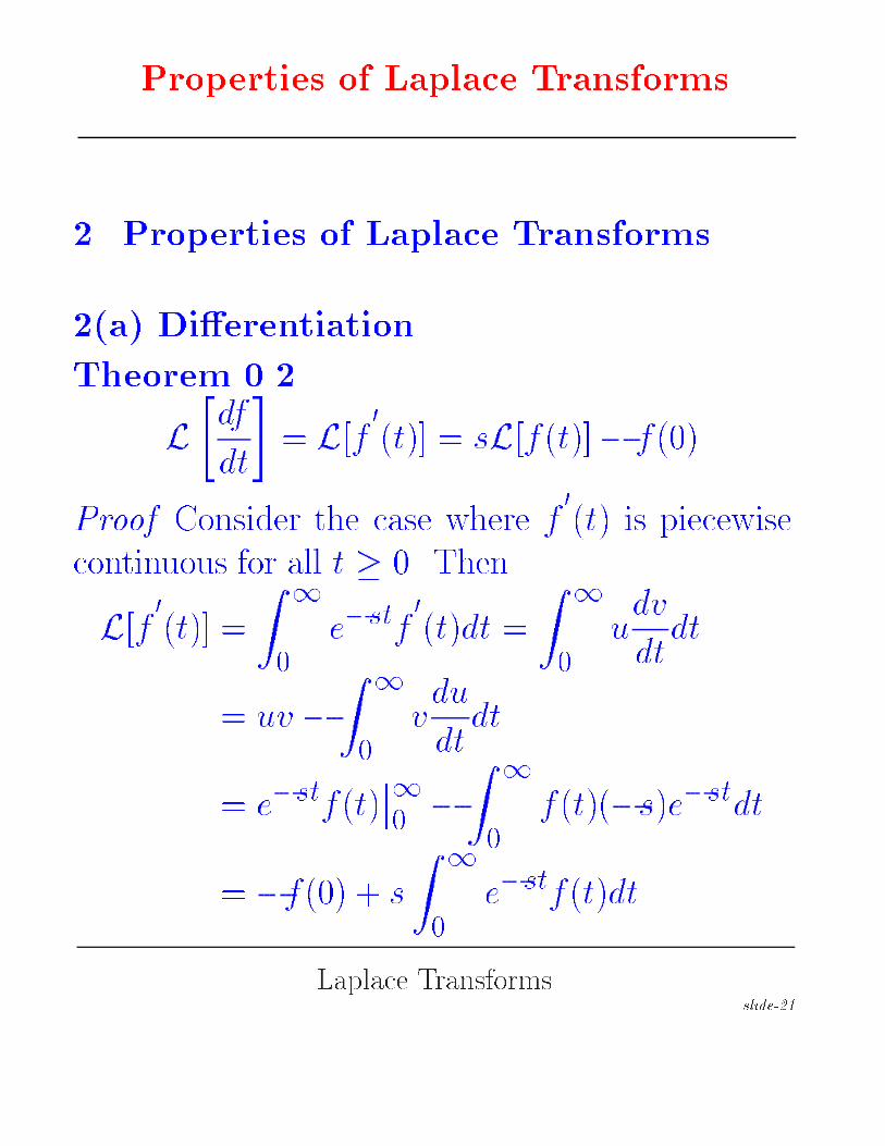
�� Properties of Laplace Transforms
�a� Di�erentiation
Theorem ����
L
�df
dt
�� L�f
�
�t�� � sL�f �t��� f ���
Proof� Consider the case where f�
�t� is piecewisecontinuous for all t � �� Then
L�f�
�t�� �
Z�
�e�stf
�
�t�dt �
Z�
�udv
dtdt
� uv �
Z�
�vdu
dtdt
� e�stf �t����� �
Z�
�f �t���s�e�stdt
� �f ��� s
Z�
�e�stf �t�dt
Laplace Transformsslide���

Properties of Laplace Transforms
Hence
L�f�
�t�� � sL�f �t��� f ���
Remark ���� Di�erentiation of a function f �t� isequivalent to multiplication of F �s� by s�
Laplace Transformsslide���

Properties of Laplace Transforms
Similarly�
L�f��
�t�� � L�d�f �t�
dt��
� sL�f�
�t��� f�
���
� s�sL�f �t��� f ����� f�
���
� s�L�f �t��� sf ��� � f�
���
� s�F �s�� sf ��� � f�
���
Extending this�
L�f���
�t�� � s�F �s�� s�f ��� � s�f�
��� � f��
���
By induction� it can be shown that
L�fn�t�� � snF �s�� sn��f ��� � sn��f���� � � � �
�sfn������ fn�����
Laplace Transformsslide���

Examples
Example ���
f �t� � t� � f�
�t� � t � f��
�t� �
f ��� � � � f�
��� � �
Using the above formula� we have
L�f��
�t�� � s�L�f �t��� sf ��� � f�
���
But
L�f��
�t�� � L� � �
sHence
s� s�L�f �t��� sf ��� � f
�
���
� s�L�f �t��
or
L�f �t�� �
s�
Laplace Transformsslide���
Properties of Laplace Transforms
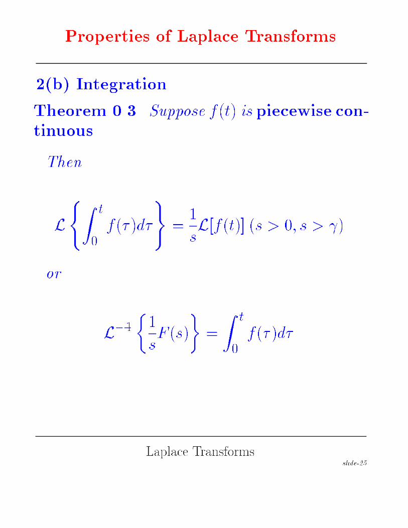
�b� Integration
Theorem ���� Suppose f �t� is piecewise con�tinuous
Then
L
Z t
�f �� �d�
�
�
sL�f �t�� �s � �� s � ��
or
L����
sF �s�
��
Z t
�f �� �d�
Laplace Transformsslide���

Properties of Laplace Transforms
Remark ���� Suppose
G�s� ��
sF �s�
First �nd
f �t� � L���F �s��
Then
g�t� �
Z t
�f �� �d�
Laplace Transformsslide���
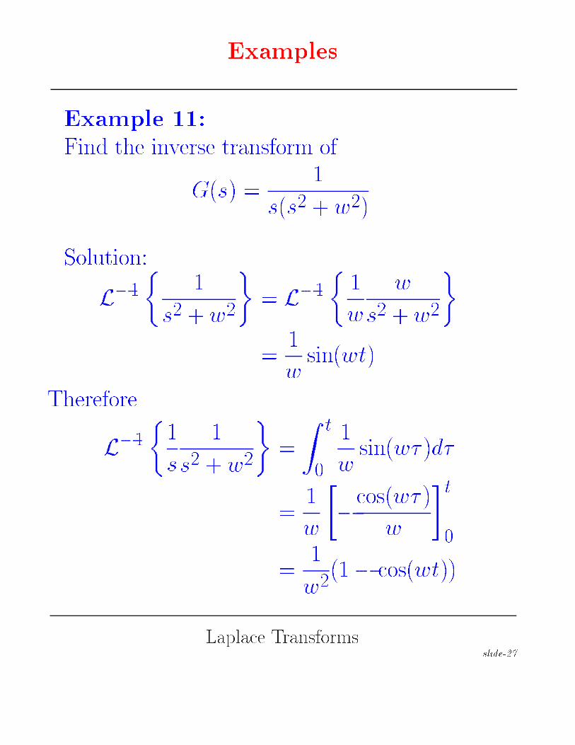
Examples
Example ���Find the inverse transform of
G�s� ��
s�s� w���Solution�
L���
�
s� w�
�� L��
��
w
w
s� w�
�
��
wsin�wt�
Therefore
L����
s
�
s� w�
��
Z t
�
�
wsin�w� �d�
��
w
��cos�w� �
w
�t�
��
w���� cos�wt��
Laplace Transformsslide���

Properties of Laplace Transforms
�c� Shifting on the s�axis
Theorem ���� Suppose
L�f �t�� � F �s�
Then
L�e�atf �t�� � F �s a�
Similarly
L���F �s a�� � e�atf �t�
Proof�
F �s a� �
Z�
�e��s�a�tf �t�dt
�
Z�
�e�st�e�atf �t��dt
� L�e�atf �t��
Laplace Transformsslide���

Properties of Laplace Transforms
Remark ���� L�T� of e�atf �t� can be found by�rst �nding the L�T� of f �t� �neglecting the factore�at� and then changing s with s a in F �s��
Remark ���� Similarly
L�eatf �t�� � F �s� a�
and
L���F �s� a�� � eatf �t�
Laplace Transformsslide��

Properties of Laplace Transforms
Example ���Given
L�sin�wt�� �w
s� w�
Then
L�e�at sin�wt�� �w
�s a�� w�
Example ���Given
L�cos�wt�� �s
s� w�
Then
L�e�at cos�wt�� ��s a�
�s a�� w�
Laplace Transformsslide��

Properties of Laplace Transforms
�d� Shifting on the t�axis
Theorem �� � Suppose
L�f �t�� � F �s�
Then
L�f �t� a�u�t� a�� � e�asF �s�
or
L���e�asF �s�� � f �t� a�u�t� a�
Remark ���� f �t�a�u�t�a� describes the resultof translating f �t� to the right by an amount a andsetting the function to zero for all t � a�
Laplace Transformsslide���

Properties of Laplace Transforms
1
1
1
u(t-1)
=
1
f(t-1)u(t-1)
f(t)
t t
t
Laplace Transformsslide���
Properties of Laplace Transforms
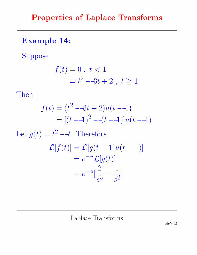
Example ���
Suppose
f �t� � � � t � �
� t� � �t � t � �
Then
f �t� � �t� � �t �u�t� ��
� ��t� ��� � �t� ���u�t� ��
Let g�t� � t� � t� Therefore
L�f �t�� � L�g�t� ��u�t� ���
� e�sL�g�t��
� e�s�
s��
�
s��
Laplace Transformsslide���

Properties of Laplace Transforms
Consider the following di�erent functions ��
�� f �t� t��
� f �t� t��u�t�
�� f �t�u�t� t��
�� f �t� t��u�t� t��
All the functions are di�erent�
Let f �t� � sin�wt��
Laplace Transformsslide���
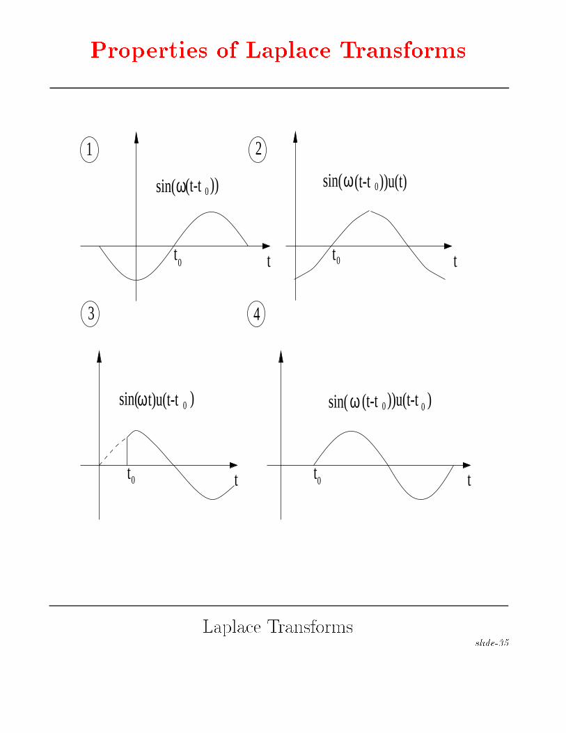
Properties of Laplace Transforms
sin(ω(t-t ))0
sin(ωt)u(t-t 0 )
sin(ω(t-t ))u(t)0
ωsin( (t-t ))u(t-t0 )0
t t0
t tt t
t t0
0 0
1 2
3 4
Laplace Transformsslide���

Properties of Laplace Transforms
Example � �
Find the L�T� of the three functions �graphs ��� and ���
Graph ��
L�sin�w�t� t���u�t�� � L�sin�w�t� t����
� L�sin�wt� cos�wt��� cos�wt� sin�wt���
� cos�wt��w
s� w�� sin�wt��
s
s� w�
�cos�wt��w � sin�wt��s
s� w�
Laplace Transformsslide���
Properties of Laplace Transforms
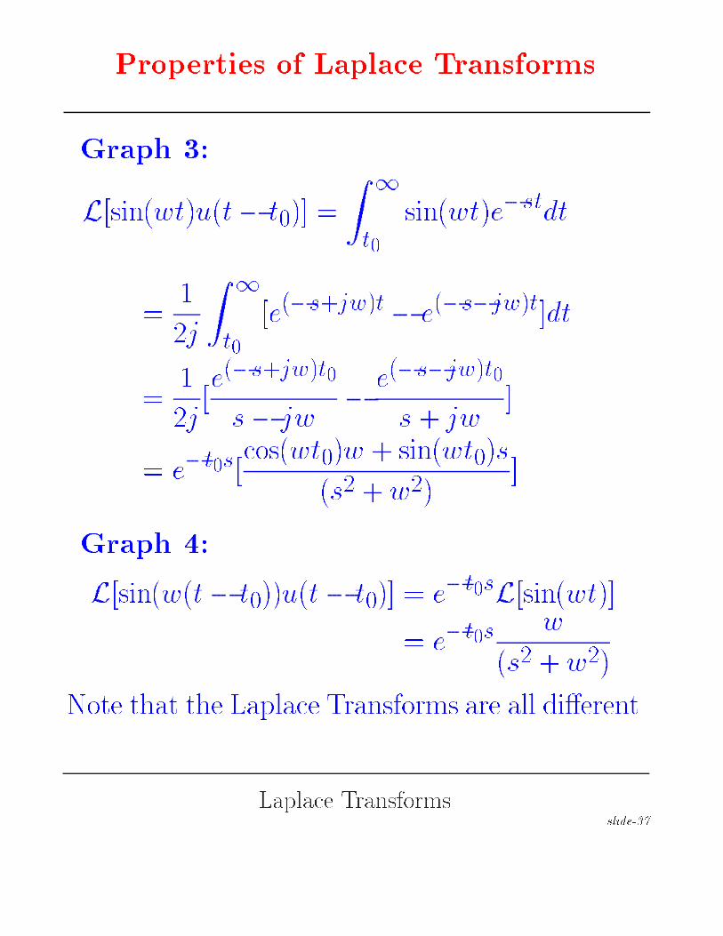
Graph ��
L�sin�wt�u�t� t��� �
Z�
t
sin�wt�e�stdt
��
j
Z�
t
�e��s�jw�t � e��s�jw�t�dt
��
j�e��s�jw�t
s� jw�e��s�jw�t
s jw�
� e�ts�cos�wt��w sin�wt��s
�s� w���
Graph ��
L�sin�w�t� t���u�t� t��� � e�tsL�sin�wt��
� e�tsw
�s� w��
Note that the Laplace Transforms are all di�erent�
Laplace Transformsslide���