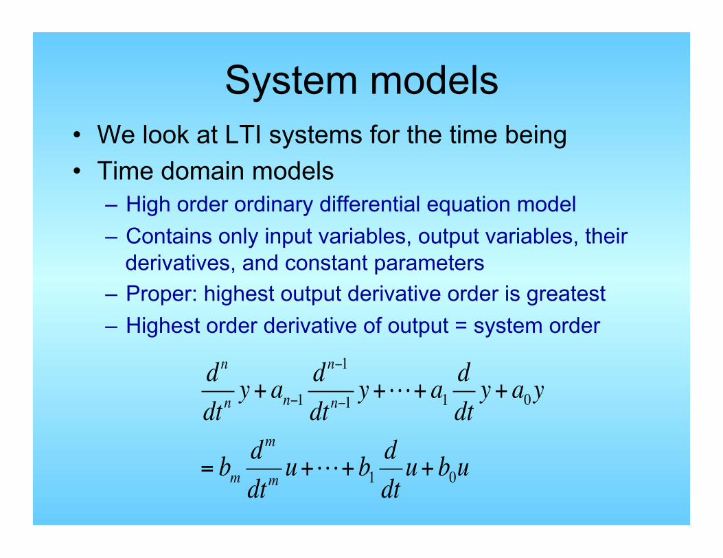
System models •  We look at LTI systems for the time being •  Time domain models

–  High order ordinary differential equation model –  Contains only input variables, output variables, their

derivatives, and constant parameters –  Proper: highest output derivative order is greatest –  Highest order derivative of output = system order

dn

dtny+ an−1

dn−1

dtn−1y++ a1

ddty+ a0y

= bmdm

dtmu++ b1

ddtu+ b0u

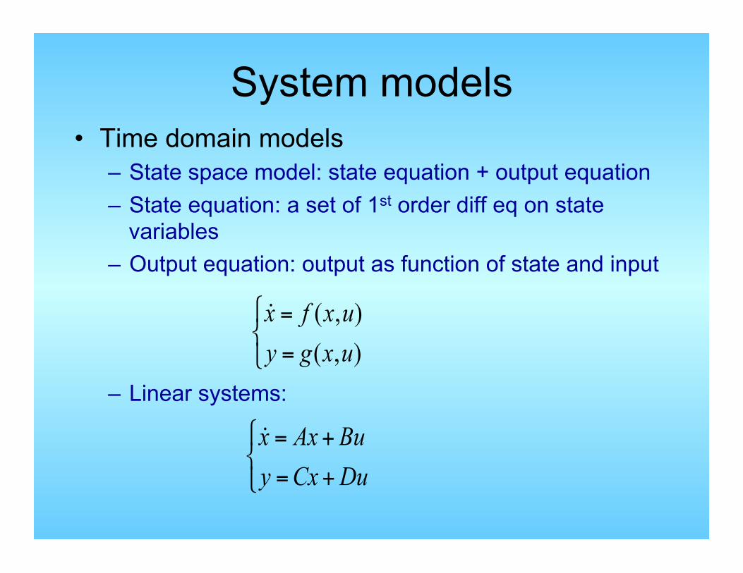
System models •  Time domain models

–  State space model: state equation + output equation –  State equation: a set of 1st order diff eq on state

variables –  Output equation: output as function of state and input

–  Linear systems:

x = f (x,u)y = g(x,u)

!"#

x = Ax + Buy =Cx +Du

!"#

uyaydtday

dtday

dtd

n

n

nn

n

=++++−

−

− 011

1

1

ODE model to State space model

Let x1 = y, x2 = y, x3 = y, ...Then x1 = x2 , x2 = x3, x3 = x4 , ...

ddt

x1x2xn

!

"

#####

$

%

&&&&&

=

0 1 0 … 00 0 1 … 0 −a0 −a1 −a2 … −an−1

!

"

#####

$

%

&&&&&

x1x2xn

!

"

#####

$

%

&&&&&

+

001

!

"

####

$

%

&&&&

u

y = [ 1 0 0 ... 0]x + [0]u

uzazdtdaz

dtdaz

dtd

zbzdtdbz

dtdby

ubudtdbu

dtdb

yaydtday

dtday

dtd

n

n

nn

n

m

m

m

m

m

m

n

n

nn

n

=++++

+++=

+++=

++++

−

−

−

−

−

−

011

1

1

01

01

011

1

1

:Then

Let

:When

ODE model to State space model

m<n

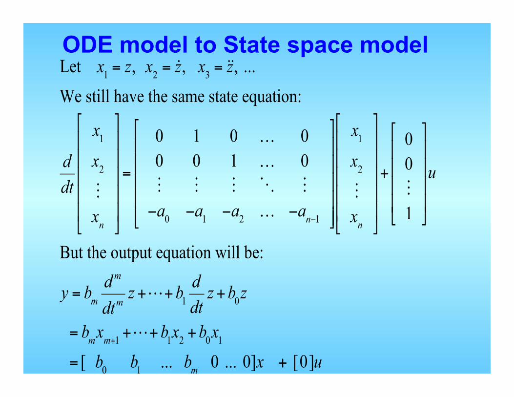
ODE model to State space model Let x1 = z, x2 = z, x3 = z, ...

We still have the same state equation:

ddt

x1

x2

xn

!

"

#####

$

%

&&&&&

=

0 1 0 … 00 0 1 … 0 −a0 −a1 −a2 … −an−1

!

"

#####

$

%

&&&&&

x1

x2

xn

!

"

#####

$

%

&&&&&

+

001

!

"

####

$

%

&&&&

u

But the output equation will be:

y = bmdm

dtmz ++b1

ddtz +b0z

= bmxm+1 ++b1x2 +b0x1

= [ b0 b1 ... bm 0 ... 0]x + [0]u

6

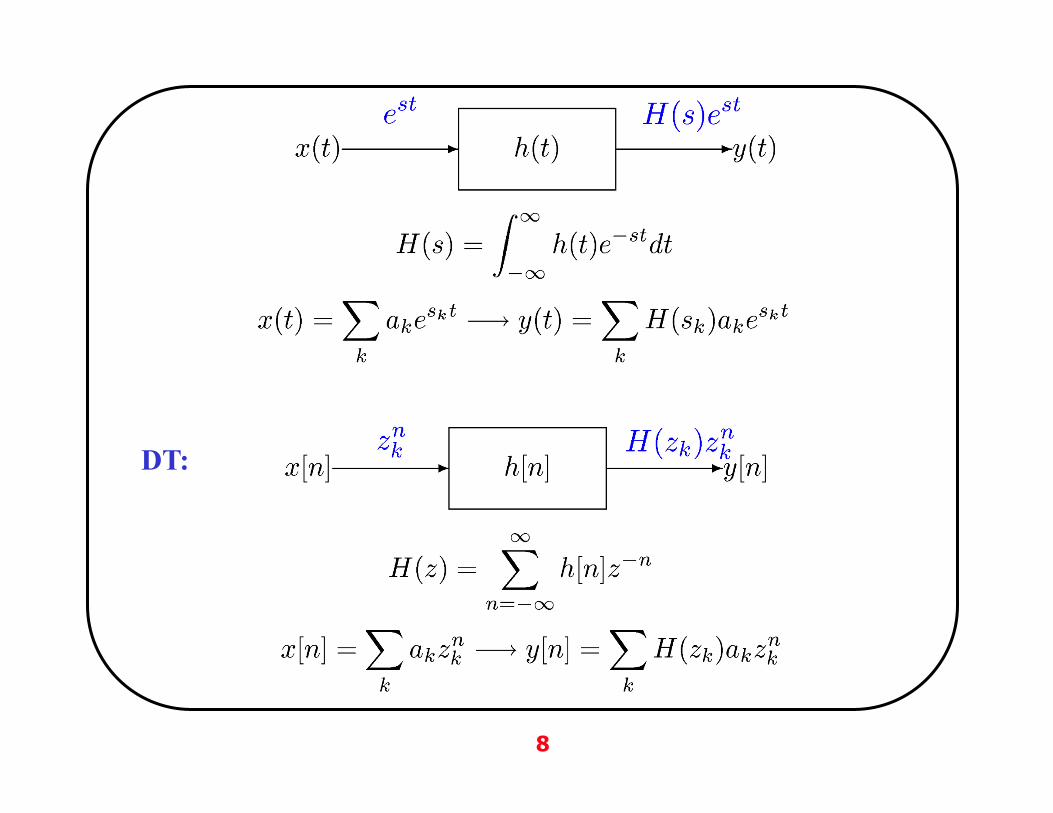
The eigenfunctions φk(t) and their properties (Focus on CT systems now, but results apply to DT systems as well.)

eigenvalue eigenfunction

Eigenfunction in → same function out with a “gain”

From the superposition property of LTI systems:

Now the task of finding response of LTI systems is to determine λk. The solution is simple, general, and insightful.

Complex Exponentials are the only Eigenfunctions of any LTI Systems

eigenvalue eigenfunction

eigenvalue eigenfunction

that work for any and all

8

DT:

9

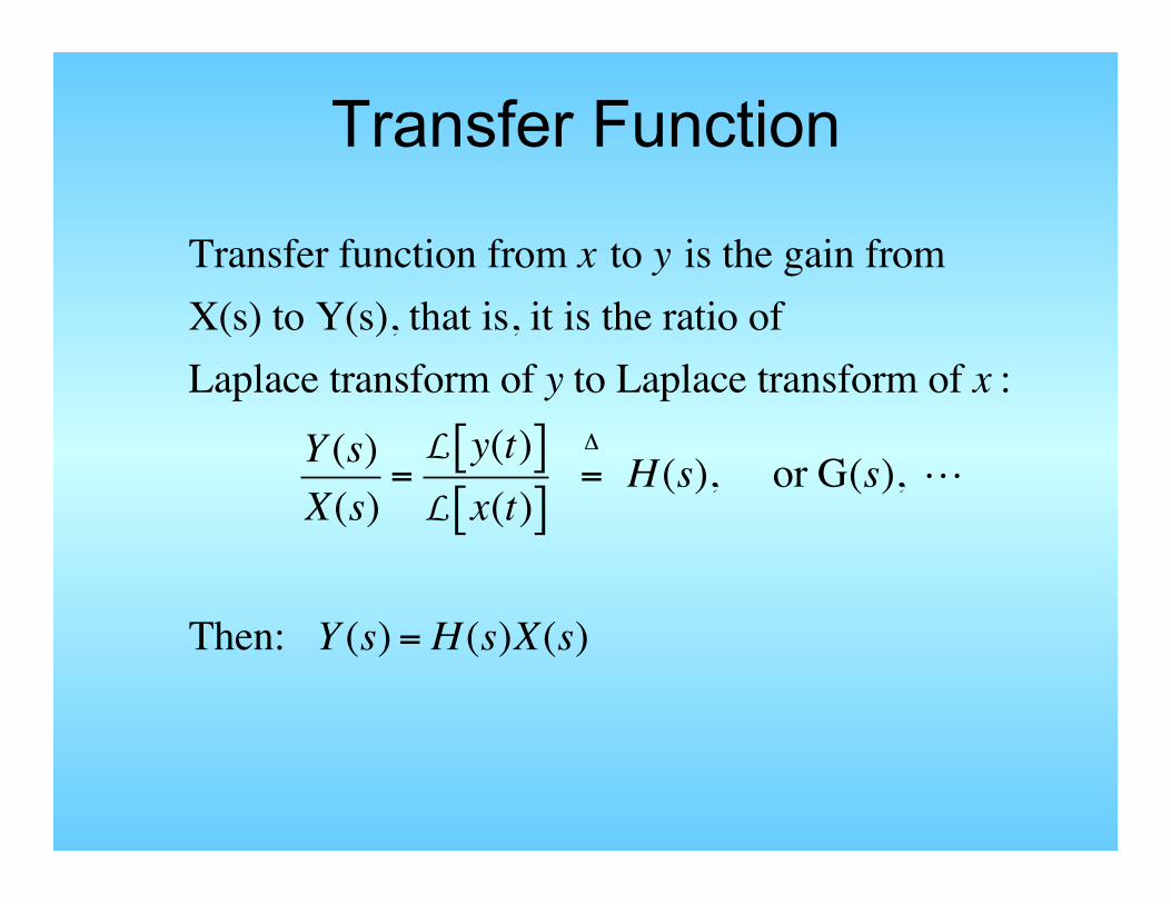
Transfer Function

Transfer Function

Transfer function from x to y is the gain fromX(s) to Y(s), that is, it is the ratio ofLaplace transform of y to Laplace transform of x :

Y (s)X(s)

=L y(t)[ ]L x(t)[ ]

=Δ

H (s), or G(s),

Then: Y (s) = H (s)X(s)

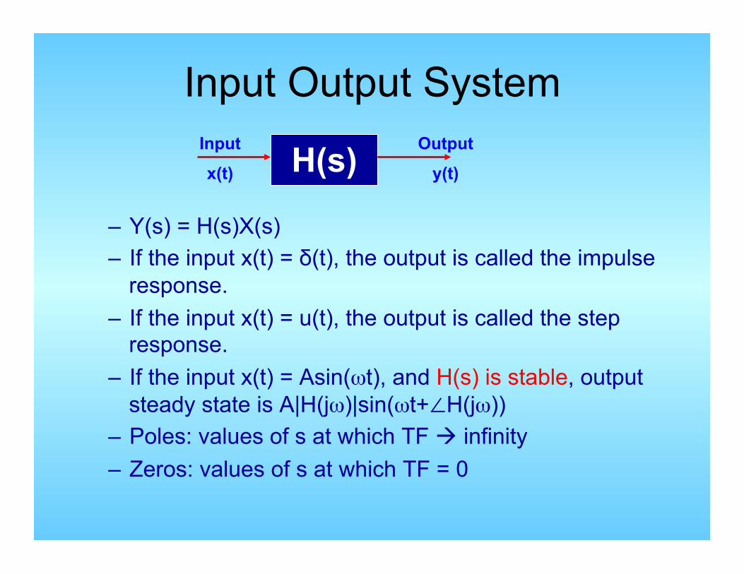
Input Output System

–  Y(s) = H(s)X(s) –  If the input x(t) = δ(t), the output is called the impulse

response. –  If the input x(t) = u(t), the output is called the step

response. –  If the input x(t) = Asin(ωt), and H(s) is stable, output

steady state is A|H(jω)|sin(ωt+∠H(jω)) –  Poles: values of s at which TF à infinity –  Zeros: values of s at which TF = 0

Input

x(t)

Output

y(t) H(s)

Example: controller

•  Proportional controller: C(s) = KP =const •  Integral controller: C(s) = KI/s •  Derivative controller: C(s) = KDs •  PI controller: C(s) = KP + KI/s •  PD controller: C(s) = KP + KDs •  PID controller: C(s) = KP + KI/s + KDs

controller C(s)

E(s) U(s)

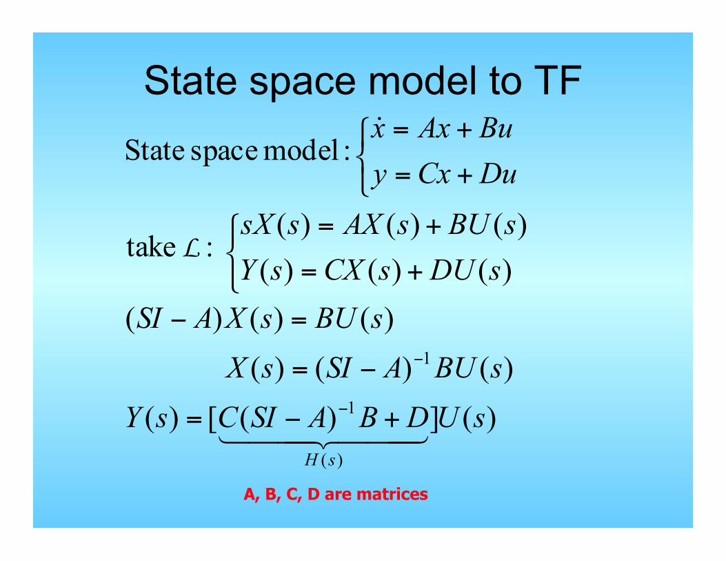
State space model to TF

)(])([)()()()(

)()()()()()()()()(

: take

:model space State

)(

1

1

sUDBASICsYsBUASIsX

sBUsXASIsDUsCXsYsBUsAXssX

DuCxyBuAxx

sH

+−=

−=

=−⎩⎨⎧

+=

+=

⎩⎨⎧

+=

+=

−

−

L

A, B, C, D are matrices

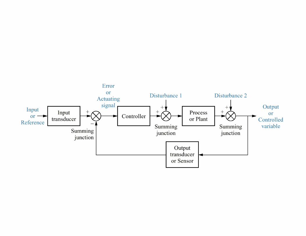
Block  diagrams  computa1ons  

CONTROLLER CONTROLLED DEVICE

FEEDBACK ELEMENT

+ ++

-

Block Diagrams •  A line is a signal •  A block is a gain •  A circle is a sum •  Due to h.f. noise,

use proper blocks: num deg ≤ den deg •  Try to use just horizontal or vertical lines

– Use additional “ ” to help e.g.

Σ

x s +

+

-

+

y

z

G x yy = Gx

z y

x s

- +

+

s = x + z - y

Σ

Block Diagram Algebra •  Series:

•  Parallel:

G1 x y

G2 G1 G2 x y

G1

x y

G2 +

+G1 + G2

x yè

è

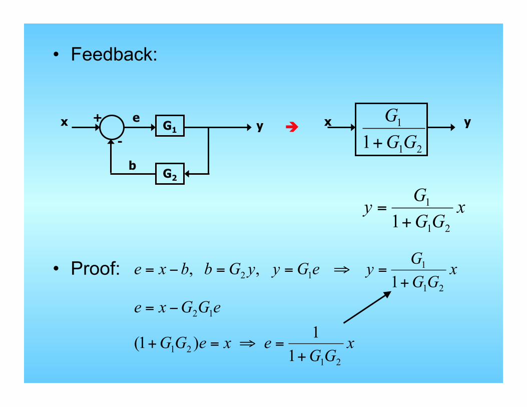
•  Feedback:

•  Proof:

xGG

Gy21

1

1+=

G1 x y

G2

-

+

b

e x y

21

1

1 GGG

+

xGG

exeGG

eGGxe

xGG

GyeGyyGbbxe

2121

12

21

112

11)1(

1,,

+=⇒=+

−=

+=⇒==−=

è

G1

G2

+

+

21

1

1 GGG

−

-

+

1

1

dn

2

2

dn 2121

21

ddnndn+

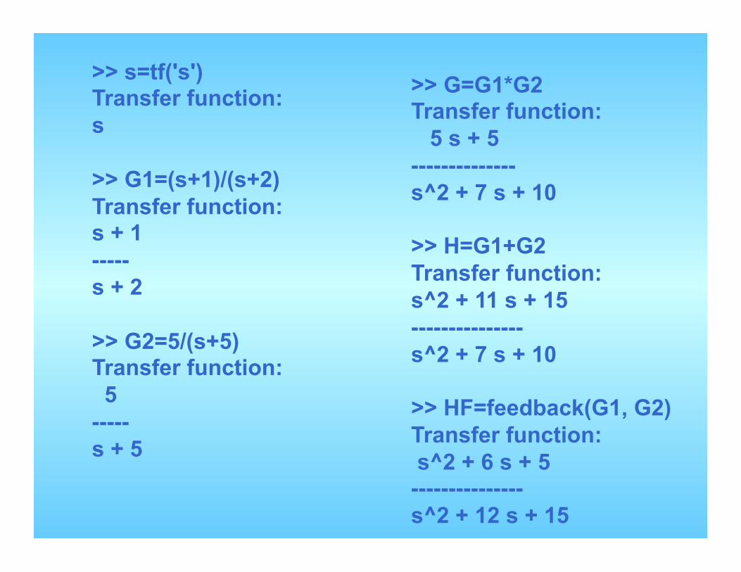
>> s=tf('s') Transfer function: s >> G1=(s+1)/(s+2) Transfer function: s + 1 ----- s + 2 >> G2=5/(s+5) Transfer function: 5 ----- s + 5

>> G=G1*G2 Transfer function: 5 s + 5 -------------- s^2 + 7 s + 10 >> H=G1+G2 Transfer function: s^2 + 11 s + 15 --------------- s^2 + 7 s + 10 >> HF=feedback(G1, G2) Transfer function: s^2 + 6 s + 5 --------------- s^2 + 12 s + 15

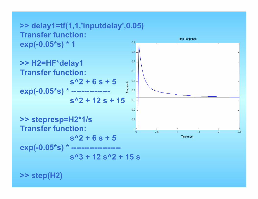
>> delay1=tf(1,1,'inputdelay',0.05) Transfer function: exp(-0.05*s) * 1 >> H2=HF*delay1 Transfer function: s^2 + 6 s + 5 exp(-0.05*s) * --------------- s^2 + 12 s + 15 >> stepresp=H2*1/s Transfer function: s^2 + 6 s + 5 exp(-0.05*s) * ------------------- s^3 + 12 s^2 + 15 s >> step(H2)

0 0.5 1 1.5 2 2.50

0.1

0.2

0.3

0.4

0.5

0.6

0.7

0.8

0.9Step Response

Time (sec)

Ampl

itude

Quarter car suspension

kbs +m1

s1R(s) y+

- s1

Series

2mskbs +R(s) +

-

yFeedback

kbsmskbs++

+2

R(s) y

kbsmskbssHTF++

+== 2)(

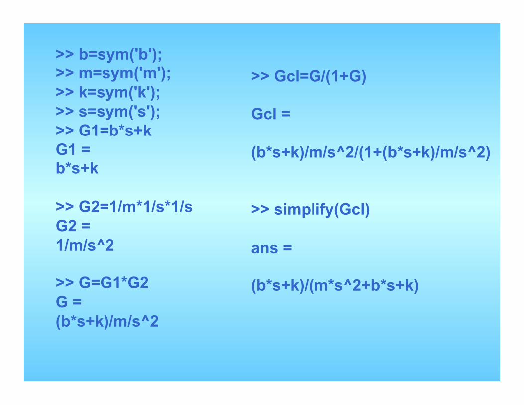
>> b=sym('b'); >> m=sym('m'); >> k=sym('k'); >> s=sym('s'); >> G1=b*s+k G1 = b*s+k >> G2=1/m*1/s*1/s G2 = 1/m/s^2 >> G=G1*G2 G = (b*s+k)/m/s^2

>> Gcl=G/(1+G) Gcl = (b*s+k)/m/s^2/(1+(b*s+k)/m/s^2) >> simplify(Gcl) ans = (b*s+k)/(m*s^2+b*s+k)

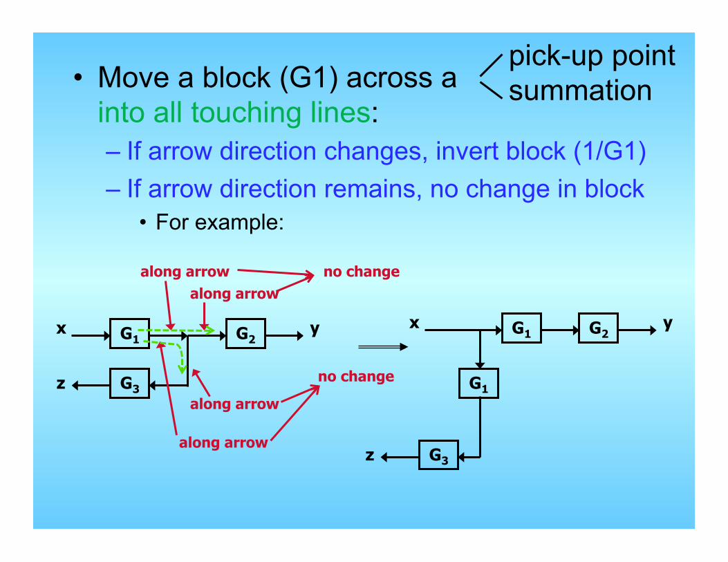
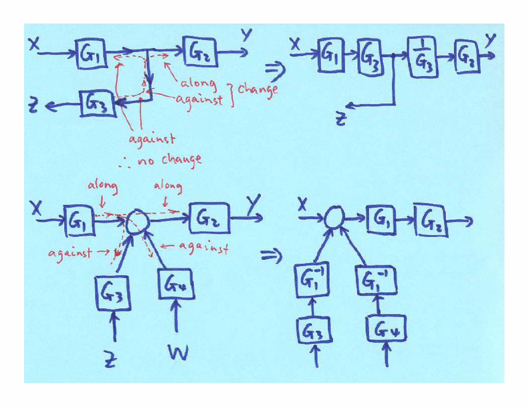
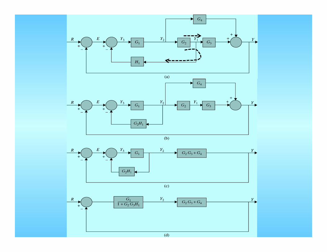
•  Move a block (G1) across a into all touching lines: –  If arrow direction changes, invert block (1/G1) –  If arrow direction remains, no change in block

•  For example:

pick-up point summation

G1 x yG2

G3 z

along arrow along arrow

along arrow

along arrow

no change

no change

G1 x yG2

G3 z

G1

G1 xy

G2

G3 z

G1 xy

G3 z

è G2

1/G2

G1 xy

G2

G3 z

è G1 x

yG2 G3

z

1/G3

against, against

against along

11

1RsL + Cs

1

22

1RsL +

U y+-

2R+-

Vc

I2

I1

11

1RsL + Cs

1

22

1RsL +

U y+-

2R+-

Vc

I2 11 RsL +

)(1

11 RsLCs +22

1RsL +

U y+-

2R+ -

11 RsL +

1)(1

11 ++ RsLCs 22

1RsL +

11 RsL +

U y+ -

2R

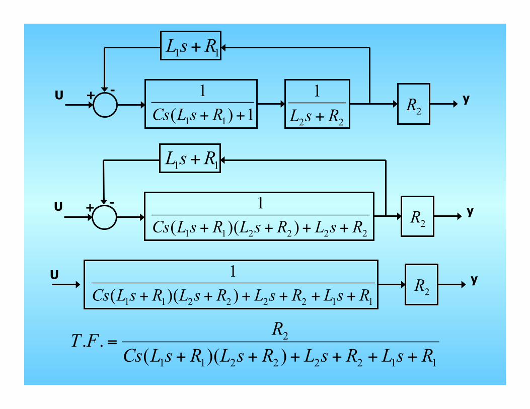
222211 ))((1

RsLRsLRsLCs ++++

11 RsL +

y+ -

2RU

11222211 ))((1

RsLRsLRsLRsLCs ++++++y

2RU

11222211

2

))((..

RsLRsLRsLRsLCsRFT

++++++=

100 12

ss+

+10( 20)s s +

U Y+

-

+

-

25s +

+

+

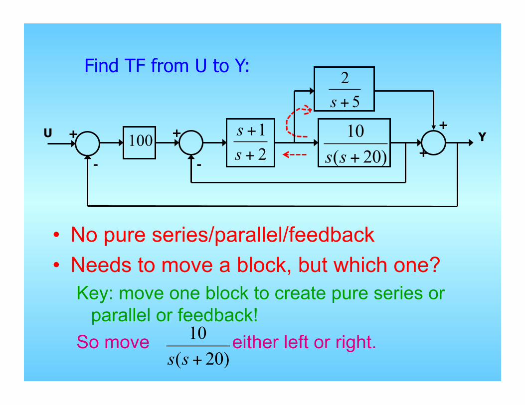
Find TF from U to Y:

•  No pure series/parallel/feedback •  Needs to move a block, but which one?

Key: move one block to create pure series or parallel or feedback!

So move either left or right. 10( 20)s s +

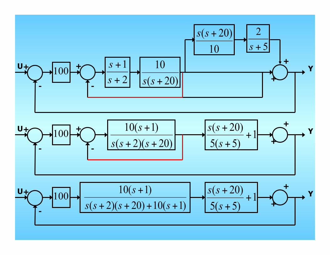
100 12

ss+

+10( 20)s s +

U Y+

-

+

-

25s +

+

+

( 20)10

s s +

100 10( 1)( 2)( 20)

ss s s

+

+ +U Y+

-

+

-

+

+

( 20) 15( 5)s ss+

++

100 10( 1)( 2)( 20) 10( 1)

ss s s s

+

+ + + +U Y+

-

+

+

( 20) 15( 5)s ss+

++

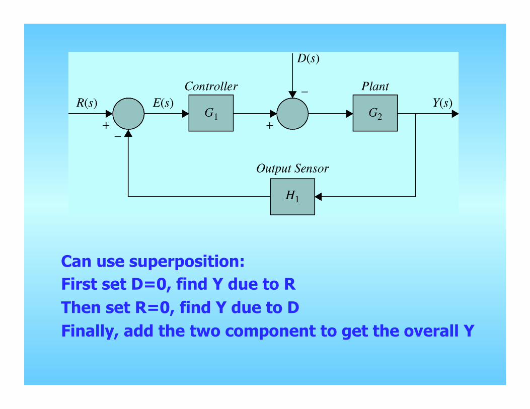
Can use superposition: First set D=0, find Y due to R Then set R=0, find Y due to D Finally, add the two component to get the overall Y

1 21

1 2 1

( ) ( )1GGY s R sGG H

=+

First set D=0, find Y due to R

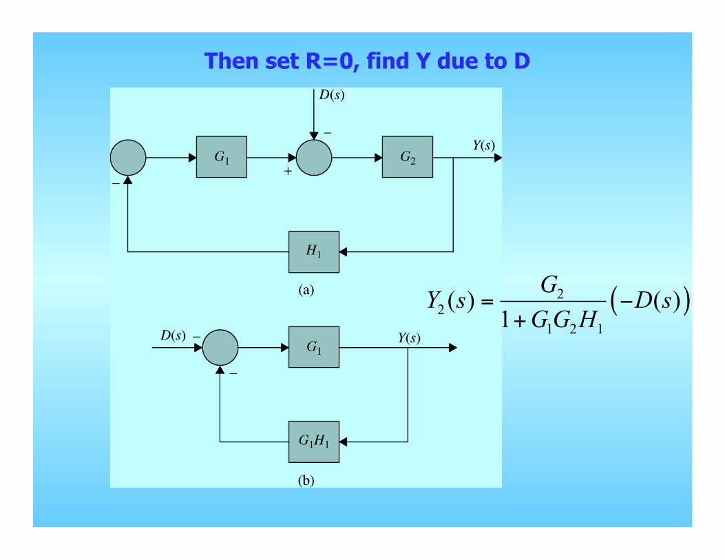
G2

( )22

1 2 1

( ) ( )1

GY s D sGG H

= −+

Then set R=0, find Y due to D

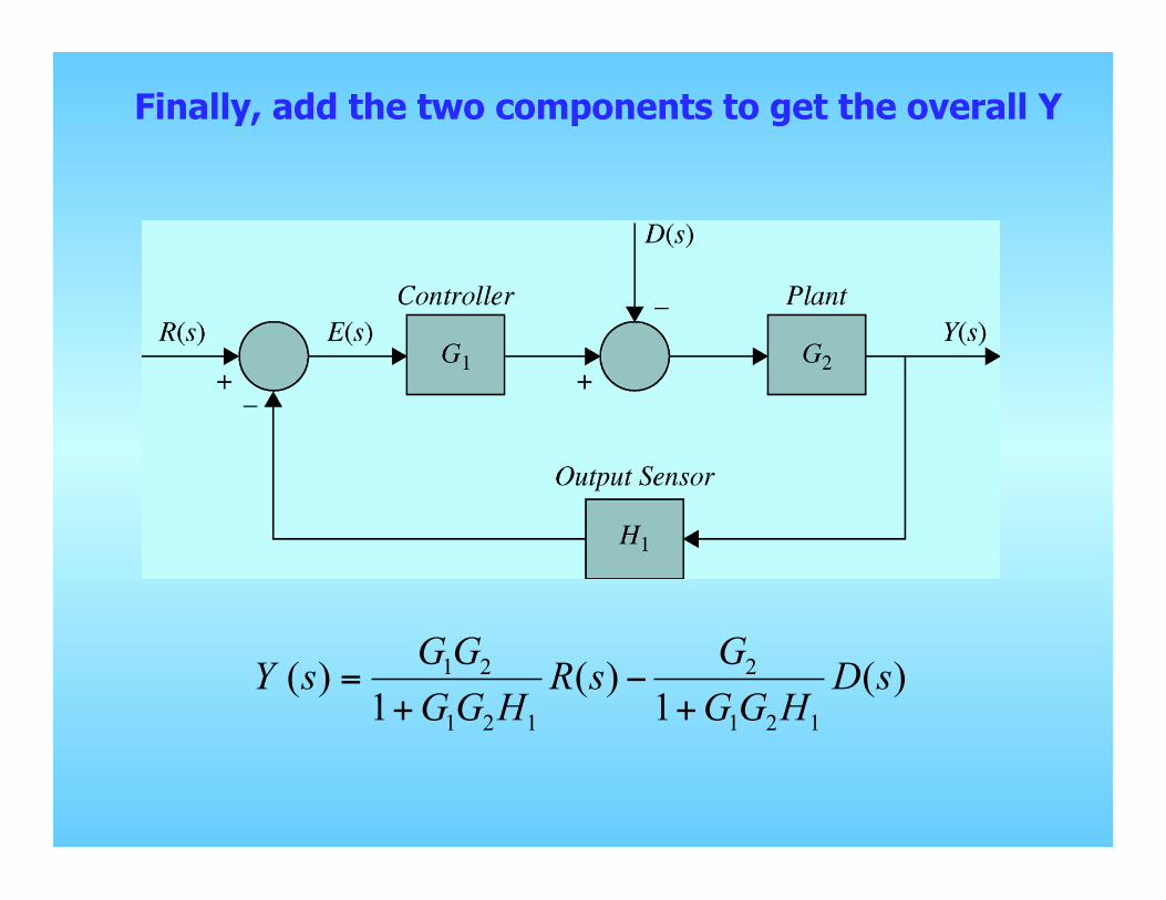
Finally, add the two components to get the overall Y

1 2 2

1 2 1 1 2 1

( ) ( ) ( )1 1GG GY s R s D sGG H GG H

= −+ +