educational and methodological complex economics
TRANSCRIPT

MINISTRY OF EDUCATION AND SCIENCE OF UKRAINE
NATIONAL UNIVERSITY OF LIFE AND ENVIRONMENTAL
SCIENCES OF UKRAINE
FACULTY OF AGRARIAN MANAGEMENT
Department of economic theory
“APPROVED”
Dean of agrarian management faculty
Ph. D, Associate Professor Ostapchyk A.D.
_________________________________
“_____” ______________________ 2020
EDUCATIONAL AND METHODOLOGICAL COMPLEX of the course
“ECONOMICS: MICROECONOMICS”
For training of educational degree “Bachelor”
Branch of knowledge 07 – Management and administration
Specialty 073 – “Management”
Kyiv – 2020
NATIONAL UNIVERSITY OF LIFE AND ENVIRONMENTAL
SCIENCES OF UKRAINE
FACULTY OF AGRARIAN MANAGEMENT
Department of economic theory
“APPROVED”
Dean of agrarian management faculty
Ph. D, Associate Professor Ostapchyk A.D.
_________________________________
“_____” ______________________ 2020
Reviewed and approved
at the meeting of Economic Theory
Protocol № 10 from 22.05. 2020
Head of department
______________________M.P. Talavyrya
WORK PROGRAM of the course
“ECONOMICS: MICROECONOMICS”
For training of educational degree “Bachelor”
Branch of knowledge 07 – Management and administration
Specialty 073 – “Management”
Faculty of Agrarian Management
Developer – Ph. D, Associate Professor Vlasenko Yu.G.
Kyiv – 2020

1. Description of the course “ECONOMICS: MICROECONOMICS”
Preparation of specialists of direction, specialty, education level
Educational degree “Bachelor”
Specialty 073 – “Management”
Branch of knowledge 07 – Management and administration
Description of the course
Species standard
Total number of hours 180
Number of ECTS credits 6
Number semantic modules 2
Course project (work)
(if available in your curriculum)
-
Form of control examination
Descriptions of the course for daily form of education external form of education
daily form of education external form of education
Year of studing 1
Semester I, II
Lectures 45
Practical, seminars 45
Laboratory classes -
Independent work 90
Individual tasks -
Number of weekly hours for daily form:
classroom
independent work of students -
4, 2
3
2. Objectives of course
The program of studying normative discipline of “Microeconomics” was draw up according to the
place and meaning of discipline in compliance with structural-logical scheme which had foreseen by the
education-professional program for “Management” specialization. It includes all content’s modules,
determined by annotation for minimal amount of lecturer hours foresaw by a standard. Subject of
Microeconomics research are economic relations between subjects of household in a conditions of scarce
resources, economic behavior of producers, consumers, owners of production and financial resources.
The primary goal of lecturing discipline “Microeconomics” is to form in future managers a
methodological base of microeconomics analysis of market subject’s behavior.
Primary tasks, which must be solved in a process of a discipline lecturing, are:
- Mastering of a universal tools of taking rational household decisions;
- Cognition of a rules of Microsystems functioning (individuals, householders, enterprises and
organizations) in a different market situation.
- Characteristic and analysis of main types of market structures – perfect competition, pure
monopoly, monopolistic competition, oligopoly;
- Determining of an influence of total market equilibrium on the effectiveness of resources
distribution in economy, exploration of reasons of scarce deficient of a market regulation, indexes of
welfare estimation, necessity of a government regulation of economy.
As a result of study of discipline a student must be correctly oriented in a general economic
situation and elect optimum ways for achievement of correct aims, to link the modern going near the
analysis of economic processes with practice of transformation transformations to Ukraine and other
countries, to lay hands on the set of economic conceptions, which will help to think in the range of public
problems and estimate economic changes which take a place in society.

Logic and structure of course “Microeconomics” will allow students to master the necessary
volume of knowledge of which enables to attain the high level of professional and economic competence
of future specialists.
A study of the course the student should:
to know: the general laws governing the functioning of the economy as a microeconomic system,
mechanisms to achieve balance in a nationwide product market, labor market, money market, the
formation of the overall balance of the national economy and the causes and factors that violation of this
balance, the economic functions of the state and the main instruments of fiscal and monetary and credit
management; relationships internally and international economic processes, instruments of state
regulation of foreign economic activity, social problems in the functioning of the national economy and
how to provide citizens with social security.
Be able to: general economic laws apply to the analysis of problems of dynamics and balance of
the national economy; investigate the causes of violations of microeconomic proportions and predict the
dynamics of microeconomic indicators, calculated on the basis of publicly available statistics inflation,
employment, unemployment, basic indicators of national accounts and to explain their dynamics; assess
the impact of micro environment on the functioning of businesses and make economically sound
solutions that take into account this effect.
3. The program of the course
Content module 1.
Market mechanism: demand and supply;
The theory of the firm: production and costs
Theme 1. Subject and method of microeconomics
Economical science takes roots from Ancient Greece as a science about ways of housekeeping. The
name consists of two parts “Oikos”- the house and “nomos”- the low. The term “economy” appeared at
the end of 5th – beginning of 4th century BC and was used by Greek philosopher Ksenophont for the first
time. For a long time, big households were named by this word. By the Ksenophont interpretation,
economy is a science about housekeeping, property and (or) movables’ managing. He thought it also as
an activity in getting money for housekeeping, etc. Later on Aristotel developed this study a lot. The term
microeconomy contains researches of economical processes at housekeeping, enterprises and
organizations. Microeconomics is tied with separate economic subjects’ activity. The subjects are
consumers, workers, investors of capital, landowners, firms – in fact any individuals or economic subjects
that play an important role at the economy functioning. Microeconomics shows why and how all the low-
level decisions are passed.
Another important aspect of microeconomics is an interaction of economic subjects at the process
of creation of bigger structures – markets of different economic branches. The subjects of the study are
market, demand and supply, costs, incomes of consumers, their distribution, etc.
Theme 2. Demand, supply and their interaction
Main instrument of positive microeconomics is the analysis of demand and supply. The curve of
supply tells about quantity of a commodity that will be presented for every price. The curve of demand
tells about what quantity of the commodity want to buy consumers for every price. When price goes up
the demand goes down cause the consumers will buy less of the commodity or won’t buy at all.
The analysis of supply and demand is used only at markets with a competition, where neither
consumers nor sellers can separately change the price.
The curves of supply. The quantity of supply (Qs) depends on market price (P). General idea of the
curve: Qs= c + dP. When the meaning of d goes up the new curve of supply will be more tilted than the
previous one cause quantity is located on the horizontal axis. When the meaning of c goes up, the curve of
supply will be on the right from the previous curve (cause of the bigger initial value on horizontal
axis.The curves of demand. The general idea of the curve:Qd = a – bp.The size of the slope is ∆Qd / ∆P =
-b.
Theme 3. Elasticity of the demand and supply
An important feature of the curves of demand and supply is sensitivity of quantity to different
changes of price. Elasticity of demand by the price is independent from the units of measurement:
Ed = P/Q ∙ ∆Q/∆P.
Elasticity of demand by incomes – is the change of the quantity of demand in percentage dependent
on the change of a price for 1%:
E1 = I/Q ∙ ∆Q/∆I,
where I – is income of a consumer.
If the price of the close product changes, the reaction of demand will be described with the help of
the cross-valuable elasticity of demand. For example, if the price of oil goes up for 1%, the demand for
natural gas (percent) will be:
EQgPo = Po/Qg ∙ ∆Qg/∆Po,
where Qg - quantity of demand for natural oil, Po - price for oil. Cross-valuable elastisity of demand
is a positive value when both products are substitutes, and negative when these products are supplements.
Elasticity of supply by the price – is the change of the quantity of supply (percent) when price
changes for 1%:Es = P/Qs ∙ ∆Qs/∆P.
Theme 4. Consumer’s behavior
Consumer’s behavior is researched by comparison of market baskets with different sets of two
products. At first we should examine interests that illustrate the variance of consumer’s choice, who
doesn’t worry about the price of different variants of choice. To understand the essence of such likings we
should compare two different baskets of consumer’s products.
Following suppositions are the base of the theory of consumer’s likings:
1) Completion – consumer likes one basket more than another from any market baskets or he doesn’t
care about which one to choose.
2) Transitivity – if there are three market baskets, if the consumer likes the first one better than the
second one, and then the second more than third one, so the first one is better than the third basket
for the consumer.
3) “More – better” – the consumer likes the basket with bigger quantity of products.
If there are only two products at the basket, the consumer’s likings can be shown at the form of a
graph. It is called the curve of indifference. This curve unites all the baskets that are indifferent for the
consumer.The curves of indifference illustrate only ordinal number of likings, cause anyway the basket
that is on top is the best for the consumer.
Theme 5. Individual and market demand
Analysis of individual and market demand is based on the model of the consumer’s behavior.
The curves of demand illustrate the changes of the best basket during the change of a budget line.
If the price goes down the budget line shifts around its axis. The curve “price – consumption” unites
a point of touch of the curves of indifference and the budget line. The curve of demand shows the
quantity of a product by every price for this product.
If the level of income changes the budget lines make the same. The curve “income – consumption”
unites points of touch of the curves of indifference to budget lines. The Angel’s curve illustrates the
quantity of product during the change of the income level. The consumption grows with an income for a
normal product. So, the curve smoothly goes up. The consumption of secondary product decreases when
the income goes down and the Angel’s curve smoothly goes down.Reduction of the price has two
consequences: profit effect and substitution effect.

Theme 6. Theory of a firm: production
This theme is dedicated to the production of a firm that is a physical connection that shows how do
the outdoing resources (factors of production, such as labor, capital and materials) become production
(for sale at market). The technology is drown by the function of production Q = F (K, L), that gives
information about maximal volume, that can get a firm if it has some capital and labor. The function of
production causes technological effectiveness – the firm produce maximum it can in such case.
Production function can be shown in two dimensions as isoquants. Isoquant is a curve, where
different combinations of resources give opportunity to produce the same quantity of production.
Isoquants are like the curves of indifference, but the volume of production can be measured and
controlled, but you can’t measure at quantitative units.
It’s important to tell long-run period of production from a short one. The difference is not only at
time but resources. Short-run period is a period of time when you can’t change one or more resources.
The firm owns some fixed resources at the short-run period. Long-run period is a period when all
resources can be changed. The period is different for different firms and branches of economy.
Theme 7. Production costs of a firm
Any production needs costs of resources that are limited and have a price. That’s why production
costs or expenditures are considered to be the value of resources (in money) that are used for the
production. Using a resource for one production we can’t use it for another. Economic costs of any
resource are equal to its price or value for the best usage. Economic costs of a resource are all the costs
caused by specific usage of the resource. It can’t be used in any other production process. For a separate
firm, economic costs are the payments though pay or incomes to give to the supplier of resources to keep
them at one production.External costs – are straight money payments to the suppliers of the productional
factors.
Internal are the costs for the resources that are the property of the firm. Using these resources in a
better way the payments can be received. One of the elements of internal costs is normal income. Normal
income is an income for internal costs of the owner’s capital. Normal income also can be payments for
managing skills. If normal income is absent at the production, businessman can reorganize the production
or close it at all.
There are fixed and variable costs at short-run period. Long-run period has only variable costs.
Content module 2.
The theory of market structures: market of product;
Markets of the factors of production
Theme 8. Perfect competitive market
As a rule in the basis of every firm behavior is profit-maximization. This means, that firms are
trying to find the best usage for its resources.
Competition in the market for investment capital requires from the firm the skill of effective capital
usage. Revenue is the price of one unit of a product, multiplied the quantity bought (TR=P*Q).
As a firm on the perfectly competitive market has no influence on the market price, so every unit
sold gives the same sum of additional or marginal revenue to the firm (MR=ΔTR/ΔQ). In this formula
MR is marginal revenue; ΔTR is the increase in total revenue; ΔQ is the increase in quantity of the
product. For separate firm marginal revenue is just the market price. Average revenue is calculated as:
ATR=TR/Q. Profit equals total revenue subtracting total costs (Π=TR-TC). We need to differ economic
and accounting profit.
Economic profit is a difference between total revenue and economic costs.
Theme 9. Monopoly Market
The direct opposite to perfect competitive market is monopoly and monopsony. Monopoly is the
availability of only one seller and many buyers on the market; and monopsony is the availability of
only one buyer and many sellers on the market.
Pure monopolist is the only seller on the market. So its demand curve is the market demand curve.
Monopolist is in the unique situation as he is the market by itself and that is why it entirely controls the
quantity of products produced for sale.
To maximize profit monopolist at first has to define peculiarities of market demand and also its own
expenditures. Data about demand and expenditures play the leading role in making economic decisions by
the firm. For maximizing profits monopolist chooses such a quantity of production, for which marginal
costs are equal to marginal revenue. But as the marginal revenue curve always lies below the demand
curve of the monopolist, the monopolist establishes price above the point of intersection of MC and MR
curves. So due to such exceeding of price over marginal costs the monopolist gains additional profit.
Theme 10. Market of Monopolistic Competition
Market of monopolistic competition is the industry, in which there are several firms. There are
not so many firms as on perfectly competitive market, but enough for that every firm could do not take
into account the actions of competitors, and there were no secret unions with the aim of production
reduction and price increase.
Differentiated goods characterize monopolistic competition. Very firm produces a good, which is a
little different than a competitor’s good. Consumers prefer goods of certain producers and to some extent
pay higher price for this good to satisfy their wants.
Market of monopolistic competition has two important peculiarities. Firstly, firms compete with
each other sailing differentiated goods, which can be easily substituted by each other, but they are not
absolutely substitutes. Secondly, entry into the market and exit out of it are free: it is not difficult for new
firms to enter the market with their own trademarks and it is as easy for acting firms, whose goods
became unprofitable, to leave the market.
Theme 11. Oligopoly
The main characteristic of oligopoly is the availability of not many firms on the market. Oligopoly
model comprises a large sphere, which is in the diapason between pure monopoly on the one hand and
monopolistic competition on the other hand. In conditions of oligopoly goods may be diversified or
homogeneous. Almost all goods are produced by a small number of firms, as entry barriers do not let new
firms to enter the market. These are “natural” barriers, which are the main in the structure of the certain
market. Moreover “old” firms (which have already divided the market between themselves) can use
strategic actions to shut the entry into the market.
While making decisions on the oligopoly market every firm must consider the reaction of its
competitors, knowing that they also consider its reaction on their decisions. The main concept of strategic
behavior analysis is the equilibrium by Nash. According to this equilibrium, every firm maximally
realizes its abilities, knowing what its competitors are doing. That’s why no-one firm has incentive to
change its course of activity.
Theme 12. Derived demand formation
Till now we dealt with markets with enterprises-producers, sellers of goods and services, population
as a final buyer of the goods. But for production of goods and services we need economic resources
(factors of production).

The firm’s demand for factors of production is determined by the consumer’s demand on full
products markets, that is why demand for factors of production is called derived demand.
The utility of factor for the firm is in the income increase, caused by the usage of this factor. As
income is realized on the market of goods, the utility of factor so as the demand for it depends not only on
the situation on the factor’s market, but also on the state of goods market.
The analysis of functioning of markets of factors of production is done according to the principles
same as on the markets of goods. Considering the type of market structure, economists study the
formation of demand for factors (individual and market) and what determinants influence the supply.
Theme 13. Labor market
Demand for factors of production (resources) is derived from the demand for goods and services,
which are produced with the help of these factors. That is why the demand for labor is determined by the
productivity of a certain kind of labor and by the level of prices on goods, in production of which it is
used.
In the conditions, when labor is the only variable resource, demand for it of a separate firm is
determined by the size of marginal product of labor in money measurement (MRPL). In general it equals
the multiplication of marginal productivity of labor and marginal revenue of the firm. For perfectly
competitive sale, at which the price equals the marginal revenue, it equals the multiplication of marginal
productivity of labor and price of the good. No matter, competitive market of products is or not, if the
firm buys resources on competitive market, MRPL curve is a curve of this firm demand for labor. The
firm maximizes profit producing such a quantity of goods, when MRPL equals marginal costs on labor
(MRCL) or wage (W). So the firm hires work force till the point where MRPL=W.
Theme 14. Capital Market
Capital is the resource of durable usage and is created with the aim of production of more goods and
services. There is an important difference between capital and other productive resources, which is a time
factor. Usage of labor gives immediate revenue to the firm, and machines, created today, will bring
revenue during many years.
When a firm makes a decision to build a plant, it has to compare the investment of capital, which is
necessary to be done today, and additional revenue, which new capital will bring in future. To evaluate
the cost of future revenues the term of “present discounted value (PDV) ” is used. PDV of one hryvnya in
n years equals 1 hrn. / (1+c)n, where C - percentage rate. From this main ratio we can define PDV of any
sum, received in any number of years.
Percentage rate is a price, which is paid for capital owners for usage of their borrowed for a certain
period of time means. Percentage rate is defined as other prices according to the equilibrium between
supply of money and demand for them. There are many factors, which influence the competitive
magnitude of percentage rates. They are: level of risk while giving the credit, term for which the credit is
being given, its size. Nominal (in current prices) and real (considering the inflation) percentage rates are
distinguished.
Theme 15. Aging, Social Security, and Health Care
In recent decades, economists have devoted a great deal of attention to understanding the economics of
the family. One area of particular interest is the decision of households to have children. In developed
economies, children provide consumption benefits for their parents (well... except when they are
teenagers). Children provide labor services on family farms and provide old-age security for their parents
in less developed economies.
From the 1960s onward, though, fertility rates declined. One of the major reasons for this is the increase
in female wage rates and labor market opportunities. Higher wages and improved job opportunities for
married women substantially raised the opportunity cost of having children. (In the diagram above, this

would be indicated by a reduction in the supply curve for children.) As wage rates for married women
have continued to increase, fertility levels have remained substantially lower than in earlier periods.
Rising divorce rates and increased educational attainment by women, have also helped to maintain low
fertility levels.
The large baby-boom generation, combined with low fertility rates in recent decades, have resulted in a
potential problem for the social security system. As the baby-boom generation retires, there will be
substantially fewer workers supporting each Social Security recipient. This problem is exacerbated by
increased longevity resulting from improvements in medical care. The problems associated with the
future of the social security system are covered in a fair amount of detail on the web page on Social
Security that I've constructed for South-Western College Publishing.
Theme 16. Government and Market Failure
This chapter addresses the major types of market failure that provides an economic rationale for
corrective governmental action:
Externalities
Externalities are side effects of production or consumption that impose costs on or provide benefits to
third-parties who are not directly involved in the activity. Positive externalities are side-effects that
provide benefits to one or more third-parties, while negative externalities harm others.
Social marginal benefits exceed private marginal benefits when positive externalities are present. Since
people do not take external benefits into account when weighing their own private benefits and costs,
social marginal benefits exceed social marginal cost at their optimal level of the activity.
Solutions to externality problems
One method of dealing with externalities is to impose a tax (in the case of a negative externality) or
provide a subsidy (in the case of a positive externality). If the tax (or subsidy) is set at the level of the
marginal external cost (or marginal external benefit), individuals will select the optimal level of the
activity since thgeir own costs and benefits now reflect social costs and benefits. This method of
correcting for the presence of an externality was first suggested by A. Pigou, and is known as a Pigovian
tax (or subsidy). This type of approach is said to "internalize the externality" by converting an external
cost or benefit into an internal cost or benefit.
The Coase theorem suggests that, as long as property rights are well established and there are no
transaction costs, private bargaining may correct for the presence of externalities. In practice, however,
the existence of transaction costs makes it unlikely that an efficient outcome will occur in the absence of
government intervention.
Public goods
A public good is a good that is nonrival in consumption. This means that one person's consumption does
not reduce the quantity or quality of the good available to other consumers. Examples of public goods
include national defense and TV and radio signals broadcast through the air. Some public goods have
some congestion costs in which the benefits do decline a bit as the number of people consuming them
rises. Town parks, highways, police and fire protection, and other similar commodities and services fit
this definition.
Asymmetric information occurs in this case because the buyer of a used car has less information about the
true quality of the car than does the seller. The equilibrium price of a 1-year old used car reflects the
average value of these cars. Those who try to sell high-quality used cars end up with the same price that
sellers of "lemons" receive since buyers cannot tell them apart. The government may attempt to correct
for adverse selection by requiring product warranties.

4. Structure of the course
specialty 073– “Management”
Titles content modules and themes
Amount of hours
daily form of education
total including the
l s lab individual independent
1 2 3 4 5 6 7
Content module 1. Market mechanism: demand and supply. The theory of the
firm:production and firm
Theme 1. The subject and method of
microeconomics
12 4 4 - - 6
Theme 2. Demand, supply and their
interaction
13 4 4 - - 6
Theme 3. Elastiсity of demand and
supply
13 4 4 - - 6
Theme 4. The theory of consumer
behavior
13 5 5 - - 7
Theme 5. The individual and market
demand
13 4 4 - - 7
Theme 6. The theory of the firm:
production
13 4 4 - - 6
Theme 7. The theory of the firm: cost
of production
13 5 5 - - 7
Total for the semantic module 1 90 30 30 - - 45
Content module 2. The theory of market strukture: market of product. Markets of
the factors of production
Theme 8. The market of perfect
competitiveness
10 2 2 - - 5
Theme 9. Monopoly market 10 2 2 - - 5
Theme 10. The market of
monopolistic competitiveness
10 1 1 - - 5
Theme 11. Oligopoly 10 2 2 - - 5
Theme 12. The formation of derived
demand
10 2 2 - - 5
Theme 13. Labor market 10 2 2 - - 5
Theme 14. Capital market 10 2 2 5
Theme 15. Aging, Social Security, and
Health Care
10 1 1 5
Theme 16. Government and Market
Failure
10 1 1 5
Total for the semantic module 2 90 15 15 - - 45
Total hours 180 45 45 - - 90

5. Topics of practical works
specialty 6.030502 – “Economic cibernetics”
№
Name of the topic hours
1. The subject and method of microeconomics 2
2. Demand, supply and their interaction 2
3. Elastiсity of demand and supply 3
4. The theory of consumer behavior 4
5. The market and individual demand 2
6. The theory of the firm: production 2
7. The theory of the firm: cost of production 2
8. The market of perfect competitiveness 4
9. Monopoly market 4
10. The market of monopolistic competitiveness 2
11. Oligopoly 2
12. The formation of derived demand 2
13. Labor market 4
14. Capital market 4
15. Aging, Social Security, and Health Care 3
16. Government and Market Failure 3
Total 45
6. Test questions, tests, tasks for determining the level of learning students
6.1. Test questionsfor determining the level of learning students
1. The microeconomics.
2. Methods of microeconomic analysis.
3. Limited resources and the immensity of needs.
4. The problem of choice.
5. Matrix market forms
6. Market: essence, conditions of operation, the positive and negative sides.
7. Types markets.
8. Demand. Demand function. Changes in demand and changes in demand overall.
9. Offer. Feature offers. Changes in supply and demand in general.
10. The interaction of supply and demand. Market equilibrium.
11. The impact of the tax burden on the producer and consumer surplus
12. The concept of elasticity. Price elasticity of demand. Factors of price elasticity of demand.
13. The cross-elasticity of demand. Elasticity of demand for income.
14. The elasticity of supply. Factors affecting the elasticity of supply.
15. Basic theory of consumer behavior.
16. The usefulness. Utility function.
17. The curve of indifference. Map indifference curves.
18. Marginal rate of substitution.
19. The budgetary restrictions.
20. Determination of the equilibrium of the consumer.
21. The line "income-consumption." Engel curves.
22. The line "price-consumption" and building demand curve
23. The substitution effect and the income effect
24. Microeconomic model of the company.
25. The concept and parameters of the production function.
26. The total, average and marginal product. The law of diminishing marginal productivity.
27. The production function of two variables.
28. Isocost. The choice of a combination of production factors on the criterion of
minimizing costs. The trajectory of expansion of production of the company

29. Income and expense: definition, their total, average and marginal rates.
30. The costs in the short and long run. Economies of scale.
31. The optimal production capacity and minimum effective size production.
32. Identify and conditions of the market of perfect competition
33. Demand for products competitive firms
34. Basic approaches to determine the volume of production
35. Short-term and long-term market equilibrium in perfect competition
36. offer competitive firms
37. Perfect competition and efficiency
38. Monopoly: the nature and conditions of existence.
39. Monopoly power. Varieties monopoly.
40. Demand for product monopoly firm.
41. Demand, total income, income limit in terms of simple monoply.
42. Short-term and long-term monopoly equilibrium.
43. Indicators of monopoly power.
44. The principles of pricing in terms of monopoly power.
45. Antitrust policy.
46. Monopoly and competitive balance.
47. Social costs of monopoly power. The social cost of monopoly.
48. Oligopoly: definition, characteristics and causes.
49. The behavior of oligopolists, cooperative and non-cooperative.
50. Analysis of the relationship of two producers in statics.
51. Price War: definition, purpose and consequences.
52. Basic models of oligopolistic pricing.
53. Oligopoly and economic efficiency.
54. The model of monopolistic competition: the nature, characteristics.
55.Short equilibrium firms in monopolistychnoyi competition
56. Long-term equilibrium firms in monopolistychnoyi competition
57. Nonprice competition.
58. Monopolistic competition and its efektyvnist.
59. Market of production factors: definition, functions and features
60. Limit consumption of resources and profit maximization producer
61. Demand for factors of production.
62. Market of production factors under perfect and imperfect competition
63. Wages as the price of Work.
64. The choice between individual work and rest. Individual labor supply curve.
65. Effect of state and trade unions on wages and employment.
66. Economic rents in the labor market.
67. Capital as a resource durables
68. Discounting and enterprise investment decision
69. Formation of equilibrium in the capital market
70. The land market: the nature, supply and demand of land.
71. The land rent and its types.
72. The price of land as a discounted value
6.1.1 The coursework themes
1. The theory of rational choice of the consumer.
2. Theory of production.
3. Formation of individual and market demand.
4. The market mechanism, supply and demand and their interaction.
5. The elasticity of supply and demand.
6. The theory of the firm: production costs.
7. Production costs in the long run.
8. Equilibrium in the market of perfect competition.

9. Formation offers company and industry under perfect competition.
10. Equilibrium monopoly in the short - and long run.
11. Pricing in monopoly.
12. Monopoly power monopoly and regulation.
13. Antitrust policy in Ukraine.
14. Natural monopolies and their regulation in Ukraine.
15. Monopsony and its power in the market.
16. Nekooperovana, quantitative and pricing oligopoly.
17. The theory of value and its use.
18. Collusion and price leadership in an oligopolistic market.
19. The balance in the market of monopolistic competition.
20. Nonprice competition.
21. Demand for factors of production.
22. Supply and demand in the labor market.
23. Pricing in the labor market with imperfect competition.
24. Pricing in the capital market.
25. Supply and demand analysis of capital and investment decisions.
26. The land market.
27. Production in the long run, economies of scale.
28. Oligopolists strategic behavior and game theory.
29. The total balance of competitive markets.
30. Efficiency in exchange.
31. Efficiency in production.
32. The theory of social welfare.
33. The external effects in a market economy and their government regulation.
34. State regulation of the economy at the micro level.
35. The markets with asymmetric information.
36. Choice under risk and uncertainty.
6.2. Tests for determining the level of learning students
1. Marginal revenue is calculated by the formulas …..
2. If a good is inferior and its price increases
a. the income effect will be positive and the substitution effect will be positive.
b. the income effect will be negative and the substitution effect will be negative.
c. the income effect will be positive and the substitution effect will be negative.
d. the income effect will be negative and the substitution effect will be positive.
3. The price factors of demand are …….
4. If a good is normal and its price decreases
a. the income effect will be positive and the substitution effect will be positive.
b. the income effect will be negative and the substitution effect will be negative.
c. the income effect will be positive and the substitution effect will be negative.
d. the income effect will be negative and the substitution effect will be positive.
5. A change in the distribution of income which leaves total income constant will not shift the
market demand curve for a product providing
a. everyone has an income elasticity of demand of zero for the product.
b. everyone has the same income elasticity of demand for the product.
c. individuals have differing income elasticities for the product, but the average income elasticity
for income gainers is equal to the average income elasticity for income losers.
d. any of the above conditions occur.

6. If a consumer purchases only two goods (X and Y) and the demand for X is elastic, then a
rise in the price of X
a. will cause total spending on good Y to rise.
b. will cause total spending on good Y to fall.
c. will cause total spending on good Y to remain unchanged.
d. will have an indeterminate effect on total spending on good Y.
7. Which of the curves always has a negative slope?
a. MC
b. TC
c. ATC
d. AFC
e. AVC
f. FC
8. The curve of ……. costs intersects the curves of average total and variable costs at the
point of their lowest value
9. If goods X and Y are complements, then the cross price elasticity of demand between them
will be
a. positive
b. negative
c. zero
d. infinity
10. The X-intercept of the budget constraint represents
a. how much of good Y can be purchased if no good X is purchased and all income is spent.
b. how much of good X can be purchased if no good Y is purchased and all income is spent.
c. total income divided by the price of X.
d. a and c.
11. The point of tangency between a consumer's budget constraint and his or her
indifference curve represents
a. complete satisfaction for the consumer.
b. the equivalence of prices the consumer pays.
c. constrained utility maximization for the consumer.
d. the least he or she can spend.
12. An increase in an individual’s income without changing relative prices will
a. rotate the budget constraint about the X-axis.
b. shift the indifference curves outward.
c. shift the budget constraint outward in a parallel way.
d. rotate the budget constraint about the Y axis.
13. Determine the marginal utility of a good B in equilibrium if the marginal utility of a good
A is equal to 100 utile; price of a good A is equal to $10; price of a good B is equal to $5
a. 100 utile;
b. 50 utile;
c. 20 utile;
d. 10 utile;
e. 5 utile
14. If the price of X fails, the budget constraint
a. shifts outward in a parallel fashion.
b. shifts inward in a parallel fashion.
c. rotates outward about the X-intercept.
d. rotates outward about the Y-intercept.

15. If an individual has a constant MRS of shoes for sneakers of 3/4 (that is, he or she is
always willing to give up 3 pairs of sneakers to get 4 pairs of shoes) then, if sneakers and
shoes are equally costly, he or she will
a. buy only sneakers.
b. buy only shoes.
c. spend his or her income equally on sneakers and shoes.
d. wear sneakers only 3/4 of the time.
16. Suppose a cup of coffee at the campus coffee shop is $2.50 and a cup of hot tea is $1.25.
Suppose a student’s beverage budget is $20 per week. What is the most cups of tea the
student could buy?
a. 20
b. 16
c. 10
d. 8
17. A firm is defined as
a. a president, some vice presidents, and some employees.
b. any organization that wants to make a profit.
c. any accumulation of productive assets.
d. any organization that turns inputs into outputs.
18. A production function measures how
a. a firm transforms output into input.
b. a firm transforms inputs into output.
c. an individual maximizes utility.
d. a firm minimizes cost.
19. The marginal physical productivity of labor is defined as
a. a firm’s total output divided by total labor input.
b. the extra output produced by employing one more unit of labor while allowing other inputs
to vary.
c. the extra output produced by employing one more unit of labor while holding other inputs
constant.
d. the extra output produced by employing one more unit of capital while holding labor input
constant.
20. If more and more labor is employed while keeping all other inputs constant, the marginal
physical productivity of labor
a. will eventually increase.
b. will eventually decrease.
c. will eventually remain constant.
d. cannot tell from the information provided.
21. The factor affecting the elasticity of supply and demand …….
22. For a linear demand curve
a. the price elasticity of demand is constant for all values of P and Q
b. the price elasticity of demand decreases (becomes more negative) as Q increases
and P decreases.
c. the price elasticity of demand increases (becomes less negative) as Q increases and P
decreases.
23. If demand is elastic, a decrease in quantity will cause the total spending (P*Q) to
a. rise.
b. fall.
c. remain unchanged.
d. change in a way that cannot be determined.
24. A firm’s marginal cost curve
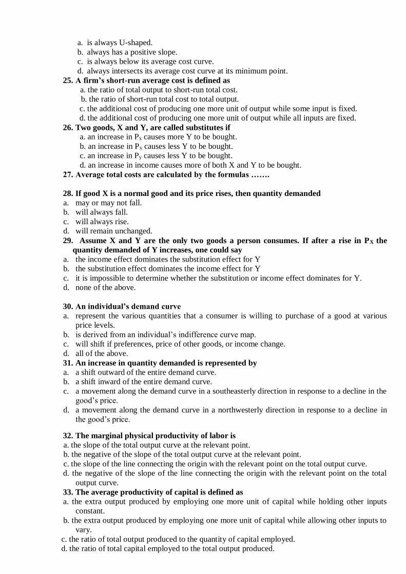
a. is always U-shaped.
b. always has a positive slope.
c. is always below its average cost curve.
d. always intersects its average cost curve at its minimum point.
25. A firm’s short-run average cost is defined as
a. the ratio of total output to short-run total cost.
b. the ratio of short-run total cost to total output.
c. the additional cost of producing one more unit of output while some input is fixed.
d. the additional cost of producing one more unit of output while all inputs are fixed.
26. Two goods, X and Y, are called substitutes if
a. an increase in Px causes more Y to be bought.
b. an increase in Px causes less Y to be bought.
c. an increase in Py causes less Y to be bought.
d. an increase in income causes more of both X and Y to be bought.
27. Average total costs are calculated by the formulas …….
28. If good X is a normal good and its price rises, then quantity demanded
a. may or may not fall.
b. will always fall.
c. will always rise.
d. will remain unchanged.
29. Assume X and Y are the only two goods a person consumes. If after a rise in PX the
quantity demanded of Y increases, one could say
a. the income effect dominates the substitution effect for Y
b. the substitution effect dominates the income effect for Y
c. it is impossible to determine whether the substitution or income effect dominates for Y.
d. none of the above.
30. An individual’s demand curve
a. represent the various quantities that a consumer is willing to purchase of a good at various
price levels.
b. is derived from an individual’s indifference curve map.
c. will shift if preferences, price of other goods, or income change.
d. all of the above.
31. An increase in quantity demanded is represented by
a. a shift outward of the entire demand curve.
b. a shift inward of the entire demand curve.
c. a movement along the demand curve in a southeasterly direction in response to a decline in the
good’s price.
d. a movement along the demand curve in a northwesterly direction in response to a decline in
the good’s price.
32. The marginal physical productivity of labor is
a. the slope of the total output curve at the relevant point.
b. the negative of the slope of the total output curve at the relevant point.
c. the slope of the line connecting the origin with the relevant point on the total output curve.
d. the negative of the slope of the line connecting the origin with the relevant point on the total
output curve.
33. The average productivity of capital is defined as
a. the extra output produced by employing one more unit of capital while holding other inputs
constant.
b. the extra output produced by employing one more unit of capital while allowing other inputs to
vary.
c. the ratio of total output produced to the quantity of capital employed.
d. the ratio of total capital employed to the total output produced.

34. Graphically, the average productivity of labor would be illustrated by
a. the slope of the total product curve at the relevant point.
b. the slope of the marginal productivity curve at the relevant point.
c. the negative of the slope of the marginal productivity curve at the relevant point.
d. the slope of the chord connecting the origin with the relevant point on the total output curve.
35. A firm's isoquant shows
a. the amount of labor needed to produce a given level of output with capital held constant.
b. the amount of capital needed to produce a given level of output with labor held constant.
c. the various combinations of capital and labor that will produce a given amount of output.
d. None of the above.
36. The marginal rate of technical substitution of labor for capital measures
a. the amount by which capital input can be reduced while holding quantity produced constant
when one more unit of labor is used.
b. the amount by which labor input can be reduced while holding quantity produced constant when
one more unit of capital is used.
c. the ratio of total labor to total capital.
d. the ratio of total capital to total labor.
37. A firm's rate of technical substitution is represented graphically by
a. the slope of the line connecting the origin with the relevant point on the isoquant.
b. the negative of the slope of the line connecting the origin with the relevant point on the isoquant.
c. the slope of the isoquant at the relevant point.
d. the negative of the slope of the isoquant at the relevant point.
38. Calculated the coefficient of cross elasticity of demand, if price increase of tea by 3%
caused an increase in the quantity demand of coffee by 6%
a. 0,5
b. 2
c. 9
d. 18
39. If TC of producing 5 units make up 1000 UAH and TFC equals – 200 UAH, what would
be ATC ?
a. 800
b. 200
c. 160
d. 40
e. 5
40. The downshifting part of the ATC in the very long run period illustrates the action of:
a. negative effect of scale
b. positive effect of scale
c. constant feedback from the scale
d. the law of decreasing marginal return from the resource.

NATIONAL UNIVERSITY OF LIFE AND ENVIRONMENT SCIENCES OF UKRAINE
EQL “Bachelor”
Specialty:
“Economic cibernetics”
Faculty of
agrarian management
Department of
Economic theory
2015 – 2016
academic year
EXAM TICKET № 1
on discipline
MICROECONOMICS
“APPROVED”
Head of the Department
(signature)
Ryduy М.М.
19 April 2016 р.
Exam questions
(максимальна оцінка 10 балів на відповідь на запитання)
1. Production possibility curve and its properties.
2. Task A firm fully monopolized production. The following information removes position of firm:
МR= 1000-20Q;
ТR= 1000Q-10Q2;
МС = 100+ 10Q.
How many products and what price it will be sold at, if: a) does a firm function as simple monopoly? b) does a firm function in the conditions of pure competition?
(максимальна оцінка 10 балів за розв’язок задачі).
Different types of tests
(максимальна оцінка 10 балів на відповідь на тестові запитання)
1. If demand is inelastic, marginal revenue will be
a. positive.
b. zero.
c. negative.
d. constant.
2. If a firm wished to maximize total revenues it should produce where
a. marginal cost is zero.
b. marginal revenue is zero.
c. marginal revenue is equal to marginal cost. d. marginal revenue is equal to price.
3. In order to maximize profits, a firm that can sell all it wants without affecting price should , produce
a. where average variable costs are minimized.
b. where marginal cost is equal to average variable costs.
c. where marginal cost is equal to price.
d. where marginal cost is a minimum.
4. If a firm is a price taker, its marginal revenue is
a. equal to market price.
b. less than market price.
c. greater than market price.
d. a multiple of market price that may be either greater than or less than one.
5. If a firm's marginal revenue is below its marginal cost, an increase in production will usually
a. increase profits.
b. leave profits unchanged.
c. decrease profits.
d. increase marginal revenue.
6. If the demand faced by a firm is inelastic, selling one more unit of output will
a. increase revenues.
b. decrease revenues.
c. keep revenues constant.
d. increase profits.
7. If the demand faced by a firm is elastic, selling one less unit of output will
a. increase revenues. b. decrease revenues.
c. keep revenues constant.
d. increase profits.
8. The factor affecting the elasticity of supply and demand………………….
9. In the state of equilibrium the consumer maximizes ……………… utility
10. Goods that have negative utility are called…………………………………
_____________________ Власенко Ю.Г.

6.3. Tasks for determining the level of learning students
Task 1
a) What is a kind of the price elasticity, if 1 % increase of the price of a good causes less than 1 %
decrease of demand?
b) If 5 % decrease of the price of a good causes 8 % decrease of supply, what is the kind of the
elasticity of supply of this good ?
c) 3% increase of the price of tea caused 6 % increase of demand for coffee. What is the cross
elasticity of demand for coffee?
d) Let’s suppose, that the price elasticity of supply of raw oil is 2,5. How much must the price
increase to cause 20 % increase in the quantity of the good produced?
Task2
1. On the following graph the demand curve shifted from D0 to D1.
What factors could cause this shift?
1) a fall in a price of the substitute good for pencils
2) a fall in a price of the complement good for pencils
3) a fall in a price of raw materials, used to produce pencils
4) a fall in consumer’s income if pencils are inferior goods
5) a fall in consumer’s income if pencils are normal goods
6) added value tax reduction.
7) wide advertising of pencils
Task 3
In every following case define if there is a shift of the demand curve or a shift along the demand
curve (a shift in the quantity demanded). Show it graphically:
a) Consumers’ expenditures rise as a result of increased sales of clocks.
b) Laundry rises a price of its services, as a result the number of clients reduces.
c) Fires on coffee plantations in Brazil causes expectations for higher prices of coffee in future.
d) Healthy way of living agitation in Northern America causes the decrease of demand for cigarettes.
Task 4 There are data about the situation in the market of videotapes.
price, money 8 16 24 32 40
demand, men units 70 60 50 40 30
supply,men units 10 30 50 70 90

Draw the graph of the demand and supply of videotapes.
a) What situation will arise in the market – excess demand or excess supply of the videotapes-if the
price is 8 per unit? What is the quantity of excess demand or supply?
b) Do the same task if the price is 32 per unit.
c) What is the equilibrium price, of the videotapes in this market
d) The increase of consumers’ income caused the increase of demand for the videotapes on 15 mln
units at every price level. What will the equilibrium price and quantity be in this case?
Task5
A demand curve on backpacks in small town is described by such equation:
Q = 600 - 2Р , the equation of supply is 5 = 300 + 4Р. What is the equilibrium price and quantity?
Task 6
A firm can offer 800 pair of sledges. At the end of the winter their sale will be impossible.
Storage of their products it is also impossible. By estimation of marketing service not one pair of
sledges will not be realized at price more than 60 UAH, if to give all sledges gratis, it is possible
to sell free 1200 pair.
Draw demand and supply curves, providing for, that a demand curve carries linear character.
What is the equilibrium price and quantity of the good?
Task 7
Show graphically, what factor causes a shift in quantity supplied and what-shift of the supply
curve.
a) as a result of the costs cutting of production producers sell more cars;
b) as a consequence of oranges retail price decrease their suplly to the market decreases.
c) The government increases excise duties on alcohol drincks.
d) As a result of new technology usage the number of firms producing PC increases.
Task 8
We will assume that three firms (A,B,C) work in industry, production which volume of is expressed by
the next graphs of supply of commodity X. Plot the curve of market supply of commodity X.
Task 9
The demand curve on a commodity is described by such equalization: Qd= 600- 4Р, The supply curve
equation is: Qs = 300+8Р. What is the equilibrium price and quantity of the good? Let’s suppose that the
price of the good is 15 grn. Use the equation to calculate the deficit which will arise.

Task 10 Demand and supply of the grain per week on the grain – exchange are characterized by the data
available in the following table:
a) What will the equilibrium price and equilibrium quantity of the grain to be?
b) Show graphically demand and supply of the good
c) Assume, that the government established the maximum price of 700 grn for one ton of the grain.
How will it influence supply, economic state of
d) enterprises and their quantity in the market?
Demand, tons Price per ton, grn Supply, tons
90 600 45
80 630 50
70 690 56
60 750 60
50 810 69
40 860 70
Task11
Price elasticity of demand on the products of agriculture is 0,25, and elasticity of demand at price
on a car is 5,0. Which industries will suffer more from falling of demand. Explain the answer.
Task 12
Assume that families in a student dormitory buy 100 kg of beef per month at price 7 UAH. Price
elasticity of demand is 0.5. Expect the quantity of consumption of beef on condition that a price on
a product will be increased on 10%.
Task 13
In a town the consumption of salt per month in summer is 200 tons. The price of 1 kg of salt is 0,35
grn. Let’s assume, that the price of salt increased to 7 grn per 1 kg. Calculate the change of
consumers’ expenditures, if the price elasticity of salt is 0,1.
Task 14
Price elasticity of demand on cameras is 0,2. That will happen with the quantity of demand for these
goods, if a price on them will be increased on 20%.
Task 15
Utility indicators of different combinations of hats and apples are shown in the table:
Quantity 1 2 3 4 5 6 7 8 9 10
Utility of hats 100 190 270 340 400 450 490 520 540 550
Utility of apples 50 95 135 170 200 225 245 260 270 275
The price for hats is 2$. The price of apples is 1$. The income is 12$.
a) Show the action of the diminishing marginal utility law.
b) Define the real income of a consumer, expressed in the quantity of hats and apples bought.
c) In the equilibrium a consumer will buy___hats and ____apples; the marginal utility of hats
is____, and marginal utility of apples is____. The total utility is____.
d) What is the value of hats, expressed in apples, and the value of apples, expressed in hats?

Task 16
Consumer A is deciding how to allocate his income among buying books and clothes. The graph
reflects consumer’s budget line and indifference curve. How the following points on the graph:
a) A point, in which A maximizes his needs
b) A point, in which A buys only books
c) A point of such bundle, buying which a consumer doesn’t spend all his income, assigned on
buying the mentioned goods
d) A point, in which A gains as much satisfaction as in point d, but which is out of his budget line
e) A point, in which A buys only clothes
f) A point which shows more attractive bundle of goods than one which is shown by the point d, but
which is out of the consumer’s budget line.
Task 17 Every week a student receive from his parents 20 grn on allowance (food and entertainment). Show
the budget line of the student for every of the following situations, signing food on the vertical axis
and entertainment on the horizontal axis:
a) The price of food (Pf) is 50 kop per unit, the price of entertainment (PH) is 50 kop per unit
b) Pf = 50 kop; PH = 1 grn
c) Pf = 1 grn; PH = 50 kop
d) Pf = 40 kop; PH = 40 kop
e) Pf = 50 kop; PH = 50 kop, but income has increased to 25 grn per week.
f) Comment budget lines d and e and compare them with budget line a.
Task 18
The consumer’s income is 8 $. The price of good A is 1$, the price of good B is 0,5$. What of the
following combinations is on the budget line?
a) 5A and 6B
b) 6A and 6B
c) 8A and 1B
d) 7A and 1B
e) 4A and 4B
show the solution graphically. Plot the the budget line if the price of the good decreased on 50 % and
consumer’s income decreased to 4 $. What combinations of goods A and B will be attainable for
consumer in this case?

Task 19 A student reads magazines and listens music on tapes. A table shows an utility which he will collect
from consumption of different amount of magazines and cassettes.
Price of magazine - a 1,5 grn., and price of tape is 7,5 grn. Let's suppose that a student buys 2
cassettes and 10 magazines.
a) How much money does the student spend on the buying such amount of tapes and magazines
b) What utility he gains from consuming such a bundle of goods
c) Plot the marginal utility curve
d) Can you define if the student maximizes his utility
e) What utility will he gain if he spends all his budget on buying tapes
f) What combination of goods maximizes the student’s utility? What is the total utility from
consuming such a combination of goods?
Quantity 1 2 3 4 5 6 7 8 9 10
Utility of
magazines60 111 156 196 232 265 295 322 347 371
Utility of
tapes360 630 810 945 1050 1140 1215 1275 1320 1350
Task 20
Imagine that you make a choice between two goods A and B, utilities of which are thown in the table.
How many units of each good should you buy to maximize the utility, if your income is 9 grn, and prices
of goods A and B are relatively 2 grn and 1 grn? Define the total utility you will get. Now imagine that in
other equal conditions the price of the good A falls to 1 grn. How many units of goods A and B will you
buy in this case? Using two combinations of price and quantity of good A (known to you) plot the
demand curve for the good A..
Units of a good 1 2 3 4 5 6
Utility of good A 10 18 24 28 31 33
Utility of good B 8 15 21 26 З0 33
Task 21
Marginal utility of commodity A is 100 utils. The price of the good a is 10$. The price of the good B is
5$. Define the marginal utility of the good B in the equilibrium.
Task 22
The firm’s Total Costs in the long-term period are in the table.
a) Determin the size of the long-term Average and long-term Marginal Costs.
b) Make the curves of the long-term Average and Marginal Costs.
c) What is the size of production when the long-term Average Costs are minimum?
The quantity of production
( units per week)
Costs
Total Average Marginal
1
2
3
4
5
6
32
48
82
140
228
352
7. Educational methods
Forms and educational methods - lectures, practical classes, independent work by students
of the course.
8. Forms of control
Forms of knowledge control system evaluation - control knowledge is made by the students'
practical work, presentations of reports, compiling module tests for the module-rating system.
Current control of student learning is at the workshops and is a preliminary control of knowledge
and skills of students posing of the problem the teacher and discussing it with students solving problems
with their discussion, solving control tasks, their inspection, evaluation.
Final control is conducted to assess learning outcomes at a certain education (qualification) level
or some of its completed stage.
Final control includes a modular form of final control after logically completed part of lectures
and practical classes and the results included in the billing summary assessment.
Semester control is carried out in the form of semester examination in the amount of training
material defined guidelines, and deadlines set by the curriculum.
Students enrolled in the correspondence, carried out according to the curriculum independent
tests, tasks which cover topics course "Macroeconomics", provided methodological guidelines.
9. Distribution points that get students
Criteria for assessment of learning tasks is one of the main ways to test knowledge and skills of
students with discipline "Microeconomics". In assessing the objectives as a basis should take the
completeness and correctness of their implementation. Please note the following competencies and skills
of students:
• differentiate, integrate and unify knowledge;
• teaching material logically and sequentially;
• use additional literature.
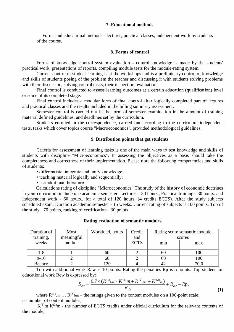
Calculations rating of discipline "Microeconomics" The study of the history of economic doctrines
in your curriculum include one academic semester: Lectures – 30 hours., Practical training - 30 hours. and
independent work - 60 hours., for a total of 120 hours. (4 credits ECTS). After the study subjects
scheduled exam. Duration academic semester - 15 weeks. Current rating of subjects is 100 points. Top of
the study - 70 points, ranking of certification - 30 points
Rating evaluation of semantic modules
Duration of
training,
weeks
Most
meaningful
module
Workload, hours Credit
and
ECTS
Rating score semantic module
scores
min max
1-8 1 60 2 60 100
9-16 2 60 2 60 100
Всього 2 120 4 42 70,0
Top with additional work Raw is 10 points. Rating the penalties Rp is 5 points. Top student for
educational work Rew is expressed by:
,)(7,0 )2()2()1()1(
RpRК
KRmKRR aw
D
mbmbm
ew
(1)
where R(1)bm … R(2)
bm – the ratings given to the content modules on a 100-point scale;
n - number of content modules;
K(1)m K(2)m - the number of ECTS credits under official curriculum for the relevant contents of
the module;

KD = K(1)m + K(2)m - number of credits ECTS, provided a working curriculum for discipline in the
current semester;
Raw, Rp - in accordance with additional work and penalties work.
,4
)(7,0 )2()1(
RpRRR
R aw
bmbm
ew
Students who had taken out educational work 60 or more points may not be an exam, and get test
scores "automatically," according to the typed number of points transferred to the national evaluation of
ECTS in accordance with table 1. in this case the top student in the discipline equal to his rating on
education.
Rd = Raw
A student wants to improve your rating and improve the assessment of discipline, it must pass
certification semester. The latter will definitely pass students who for academic work took less than 60
points. For admission to the certification a student must score at least 60 points from each module
contents and in general - not less than 42 points for academic works.
Top student certification Rat is determined on a 100-point scale. If the certification of courses a
student took less than 60 points, they will not count against him - not added to the collected points for
academic work and student remains rating (score) defined by formula (1).
Otherwise, the top student in the discipline determined Rd calculated formula:
Rd = Raw +0,3 x RAT (2)
Rate of student discipline is translated into the national assessment and evaluation of ECTS in
accordance with table .
The relationship between national and ECTS grades and rated student
National
assessment
Percentage of
students who reach
the appropriate
assessment at the
European University
Definition of assessment ECTS Students'
scores
"Fine" 10 EXCELLENT - only minor errors 90-100
"Well"
25 VERY GOOD - above the average of several errors
82-89
30 GOOD - generally work with a number of
blunders
74-81
"Satisfactorily" 25 SATISFACTORY - not bad, but with
significant shortcomings
64-73
10 SUFFICIENT - performance meets the
minimum criteria
60-63
"Unsatisfactorily" - POOR - need to work before you get credit
(positive assessment)
35-59
- POOR - thorough and elaborate 01-34
10. Methodological Support
1. Рудий М.М., Власенко Ю.Г.Мікроекономіка.Навчально-методичний посібник. -К.: ТОВ
«Аграр Медіа Груп», 213. – 246 с.
2. Мікроекономіка. Навчальний посібник для вивчення курсу.(укладачі
М.М.Рудий, Т.С.Ожелевська).К.: НАУ , 2005. – 155 с.
3. Практикум-тренінг з мікроекономіки.(укладачі М.М.Рудий та інші).К.:НАУ, 2008. -172 с.
4. Базилевич В.Д. Мікроекономіка: підручник. -К.:Знання, 2008. – 679 с.
5. Рудий М.М. Мікроекономіка. Навч.пос.-К.:Каравела, 2012. -360 с.
6. Рудий М.М., Жебка В.В. Мікроекономіка. Навч. пос.- К.: Центр учбової літератури,
2008.- 360 с.
7. Економічна теорія: Макро- і мікроекономіка / За ред. З. Г. Ватаманюка, С.М. Панчишина. –
К.: Альтернативи, 2001. – 606 с.
8. Мікроекономіка і макроекономіка: Підручник для студентів екон. спец. закл. освіти; За ред.
С. Будаговської. – К.: Основи, 2001. – 517 с.

9. Ястремський О. І., Гриценко О. Г. Основи мікроекономіки: Підручник. – К.:
Знання-Прес, 2007. – 578 с.
1. A.H. Hancen, A Cuide to Keynes, McGraw – Hill, 1953, pp. 44-54
2. A.M. Okun, “The Personal Tax Surcharge and Consumer Demand, 1968-70”, in Brookings
Papers on Economic Activity, 1, 1971, pp. 167-204
3. Andreev B.F. System a rate of the economic theory: microeconomics and macroeconomics.
The joint venture “Lenizdat”, 1998. – 574 p.
4. Economics/Richard G. Lipsey, Paul N. Courant. - 11th ed. – 1995. – 800 p.
5. J.R. Hicks. Capital and Growth, Oxford Univ. Press, 1965, Chs. 1-3 and 8
6. John Maynard Keynes, The General Theory of Employment, Interest, and Money, Harcourt
Brace Jovanovich, 1936, p. 96
7. M.M. Bober, Intermediate Price and Income Theory, rev. ed., Norton, 1962, pp. 483-95
8. Mankiw N.G. Macroeconomics. – New York: Worth Publishers, 1992. – 514p.
9. McConnell, Campbell R. Economics: principles, problems and policies / Campbell R.,
McConnell, Stanley R., Brue. – 11th ed., New York, 1990, 866 p.
10. Miller, Roger LeRoy, Macroeconomics, Harper & Row, Publishers, Inc. – 1986. – 646 p.
11. Milton Friedman, “The Quantity Theory of Money – A Restatement”, Studies in the Quantity
Theory of Money (Chicago: University of Chicago Press, 1957), pp. 3-21
12. P.A. Samuelson, Foundations of Economic Analysis, Harvard Univ. Press, 1947, pp. 311-17
13. Parkin M. Economics. – 3rd ed. Addison-Wesley Publishing Company, 1990. – 1006p.
14. Paul Samuelson and William Nordhaus. Economics. – New York: Irvin, - 1998. – 688 p.
15. Мікроекономіка і макроекономіка: Підруч. Для студентів ек. спец. закл. освіти: У 2 ч. /
С. Будаговська, О. Кілієвич, І. Луніна та ін.; За заг. ред. С. Будаговської. – К.: Вид-во
Соломії Павличко “Основи”, 2003. – 517 с.
16. Основы экономической теории: Уч.-метод. пособие / Под ред. Р.Нуреева. – М.: Вопр.
Экономики. - 1994.
11. Methodological Support
1. Піндайк Р., Рубінфельд Д. Л. Мікроекономіка / Пер. с англ. А. Олійника, Р. Скільського. – К.:
Основи, 2006. – 646 с.
2. Нуреев Р.М. Курс микроэкономики: Учебник для вуЗов. – 2-е изд., изм. – М.: Издательство
НОРМА, 2001. – 572 с.
3. Самюелсон Пол. А., Нордгауз Вільям Д. Мікроекономіка / Пер. с англ. С. Панчишина. – К.:
Основи, 1998. – 676 с.
4. Гальперин В.М., Игнатьев С. М. , Моргунов В. И. Микроэкономика: В 2-х т. / Под общ. ред.
В. М. Гальперина. – СПб: Экон. шк., 2000. – Т. 1. – 367 с.
5. Гальперин В.М., Игнатьев С. М., Моргунов В. И. Микроэкономика: В 2-х т. / Под общ. ред. В.
М. Гальперина. – СПб: Экон. шк., 2000. – Т. 2 – 503 с.
6. Талавиря М.П. Лакішик О.В. Власенко Ю.Г. Гуща І.О. Макроекономіка: Практикум-тренінг для
студентів економічних спеціальностей: Навчальний посібник. – Ніжин: ПП Лисенко М.М., 2013. –
191 с.
12. Information Resources
1. Основні макроекономічні показники / Державний комітет статистики України
[Електронний ресурс]. - Режим доступу: http://www.ukrstat.gov.ua/
2. http:www.wto.org.
3. http:/www.inf.org.
4. http:/www.bank.gov.ua.
5. Національна бібліотека України ім. В.І.Вернадського // http://www.nbuv.gov.ua
6. Офіційна Інтернет-сторінка Верховної Ради України http://www.portal.rada.gov.ua
7.Програми нормативних навчальних дисциплін підготовки бакалавра галузі знань 0306
«Менеджмент і адміністрування» напряму 6.030601 «Менеджмент». К: КНТЕУ, 2010. – с. 68-82.