Edinburgh Research Explorer

Multilateral Bargaining in Networks

Citation for published version:Lee, J 2014 'Multilateral Bargaining in Networks'.

Link:Link to publication record in Edinburgh Research Explorer

Document Version:Early version, also known as pre-print

General rightsCopyright for the publications made accessible via the Edinburgh Research Explorer is retained by the author(s)and / or other copyright owners and it is a condition of accessing these publications that users recognise andabide by the legal requirements associated with these rights.

Take down policyThe University of Edinburgh has made every reasonable effort to ensure that Edinburgh Research Explorercontent complies with UK legislation. If you believe that the public display of this file breaches copyright pleasecontact openaccess@ed.ac.uk providing details, and we will remove access to the work immediately andinvestigate your claim.

Download date: 31. May. 2018

Multilateral Bargaining in Networks

Joosung Lee∗

November 2014

Abstract

We introduce a noncooperative multilateral bargaining model for a network-restrictedenvironment, in which players can communicate only with their neighbors. Eachplayer can strategically choose the bargaining partners among the neighbors and buytheir communication links with upfront transfers. We characterize a condition onnetwork structures for efficient equilibria: An efficient stationary subgame perfectequilibrium exists for all discount factors if and only if the underlying network iseither complete or circular. We also provide an example of a Braess-like paradox, inwhich the more links are available, the less links are actually used. Thus, networkimprovements may decrease social welfare.

keywords: noncooperative bargaining, coalition formation, communication restric-tion, buyout, network, Braess’s Paradox

JEL Classification: C72, C78; D72, D74, D85

1 Introduction

Bargaining sometimes involves an agreement among three or more players. Examples

are abundant; in order to construct a railroad, a number of landowners must agree on

it; to undertake a profitable project, an unanimous agreement should be reached among

several individuals who have different but indispensable skills or resources. Sometimes

each player can cooperate with all the other players so that the unanimous agreement is

immediately reached; while other times, some players can cooperate only with a part of

other players for informational or physical reasons, and hence an gradual agreement is

inevitable.1

∗Business School, University of Edinburgh, 29 Buccluech Place, Edinburgh EH8 9JS, United Kingdom.E-mail: Joosung.LEE@ed.ac.uk. This paper constitutes the second chapter of my Ph.D. dissertationsubmitted to the Pennsylvania State University. Earlier drafts of this paper were titled “NoncooperativeUnanimity Games in Networks.” I am grateful to Kalyan Chatterjee for his guidance, encouragement,and support. I also thank Ed Green, Jim Jordan, Vijay Krishna, Shih En Lu, Neil Wallace, and theparticipants of Fall 2013 Midwest Economic Theory Meeting for helpful discussions. All remaining errorsare mine.

1Since Aumann and Dreze (1974), cooperation restrictions have been studied mainly in cooperativegames. Myerson (1977) uses a network to described the structure of cooperation restrictions.

1

1

2

3

4

5

6

7

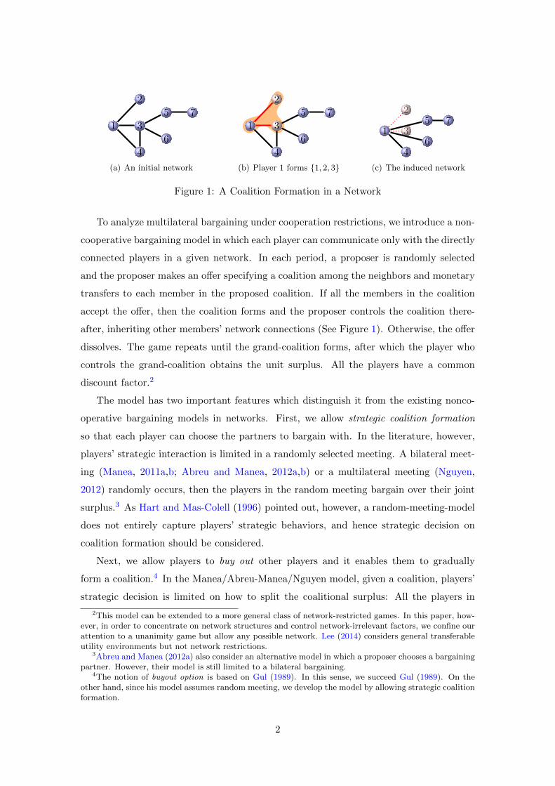
(a) An initial network

1

2

3

4

5

6

7

(b) Player 1 forms {1, 2, 3}

1

2

3

4

5

6

7

(c) The induced network

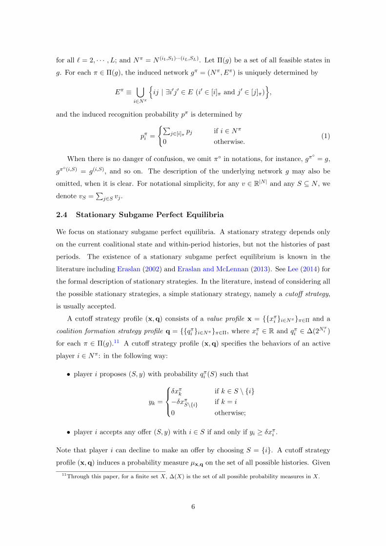
Figure 1: A Coalition Formation in a Network

To analyze multilateral bargaining under cooperation restrictions, we introduce a non-

cooperative bargaining model in which each player can communicate only with the directly

connected players in a given network. In each period, a proposer is randomly selected

and the proposer makes an offer specifying a coalition among the neighbors and monetary

transfers to each member in the proposed coalition. If all the members in the coalition

accept the offer, then the coalition forms and the proposer controls the coalition there-

after, inheriting other members’ network connections (See Figure 1). Otherwise, the offer

dissolves. The game repeats until the grand-coalition forms, after which the player who

controls the grand-coalition obtains the unit surplus. All the players have a common

discount factor.2

The model has two important features which distinguish it from the existing nonco-

operative bargaining models in networks. First, we allow strategic coalition formation

so that each player can choose the partners to bargain with. In the literature, however,

players’ strategic interaction is limited in a randomly selected meeting. A bilateral meet-

ing (Manea, 2011a,b; Abreu and Manea, 2012a,b) or a multilateral meeting (Nguyen,

2012) randomly occurs, then the players in the random meeting bargain over their joint

surplus.3 As Hart and Mas-Colell (1996) pointed out, however, a random-meeting-model

does not entirely capture players’ strategic behaviors, and hence strategic decision on

coalition formation should be considered.

Next, we allow players to buy out other players and it enables them to gradually

form a coalition.4 In the Manea/Abreu-Manea/Nguyen model, given a coalition, players’

strategic decision is limited on how to split the coalitional surplus: All the players in

2This model can be extended to a more general class of network-restricted games. In this paper, how-ever, in order to concentrate on network structures and control network-irrelevant factors, we confine ourattention to a unanimity game but allow any possible network. Lee (2014) considers general transferableutility environments but not network restrictions.

3Abreu and Manea (2012a) also consider an alternative model in which a proposer chooses a bargainingpartner. However, their model is still limited to a bilateral bargaining.

4The notion of buyout option is based on Gul (1989). In this sense, we succeed Gul (1989). On theother hand, since his model assumes random meeting, we develop the model by allowing strategic coalitionformation.

2

the coalition, once they reach an agreement, must exit the game and they are excluded

in further bargaining. Therefore, those models are not applicable to an environment in

which gradual coalition formation is inevitable to generate a surplus.5 On the other hand,

when players can buy out other players as an intermediate step, they not only consider the

surplus of the current coalition itself, but also take into account the subsequent bargaining

game. Thus players may even form a zero-surplus coalition strategically.

The main result characterizes a condition on network structures for efficient equilibria.

If the underlying network is either complete or circular, then for any discount factor

there exists an efficient stationary subgame perfect equilibrium. In such an efficient

equilibrium, each player buys out all the neighbors whenever she is selected as a proposer.

However, if the underlying network is neither complete nor circular, then some of the

players strategically delay a unanimous agreement when they are sufficiently patient.

Thus, an efficient stationary subgame perfect equilibrium is impossible for a sufficiently

high discount factor.

We also provide an interesting example in which adding a new communication link

decreases social welfare. This observation is reminiscent of the Braess’s paradox which

first appeared in Braess (1968).6 In the original context, the Braess’s paradox refers a

situation that constructing a new route reduces overall performance when players choose

their route selfishly. Analogously in our model, each player strategically chooses commu-

nication links to use for bargaining. Similarly, the more links are available, the less links

are actually used. As the result, network improvements decrease social welfare.7 To our

best knowledge, this is the first observation of an analog of the Braess’s paradox in the

bargaining literature.

The paper is organized as follows. In section 2, we introduce a noncooperative mul-

tilateral bargaining model for a network-restricted environment. Section 3 provides the

main characterization result with leading examples. Section 4 considers an alternative

model in which players cannot trade their chances of being a proposer. Missing proofs

are presented in Appendix.

5For instance, in a four-player circle, since no one can immediately form the grand-coalition, the surpluscannot be realized in their models.

6See Braess et al. (2005) for translation from the original German. In recent years, numerous stud-ies on Braess’s paradox have been made particularly in computer science and related disciplines. SeeRoughgarden (2005) for more details.

7In the Braess’s paradox with the traffic network context, all the players are worse off; while in thisbargaining in communication networks, some players may be better off even though overall performancedeteriorates.

3

2 A Model

2.1 Networks

A network (or a graph) g = (N,E) consists of a finite set N = {1, 2, · · · , n} of players (or

nodes) and a set E of links (or edges) of N . When g = (N,E) is not the only network

under consideration, the notations N(g) and E(g) are occasionally used for the player set

and the link set rather than N and E to emphasize the underlying network g. Through

this paper, we assume that g is simple8 and connected. Given g = (N,E) and S ⊆ N , a

subgraph restricted on S is g|S = (S, {ij ∈ E | {i, j} ⊆ S}). The (closed) neighborhood of

i ∈ N is given by Ni(g) ≡ {j ∈ N | ∃ij ∈ E} ∪ {i}. Let degi(g) ≡ |Ni(g)| − 1 be a degree

of i and d(i, j; g) be a (geodesic) distance between i and j in g.

A set S ⊆ N is dominating in g if, for all i ∈ N , either i ∈ S or there exists j ∈ S

such that ij ∈ E. A player i ∈ N is dominating in g if {i} is a dominating set. Let D(g)

be a set of dominating players in g. A dominating set S is minimal if no proper subset

is a dominating set. A network is trivial if |N(g)| = 1. For any integer k = 2, · · · , n− 1,

a network is k-regular if degi(g) = k for all i ∈ N(g). A network g is complete if it is

(n− 1)-regular, or equivalently if D(g) = N(g). A connected network g is circular if it is

2-regular.9

A complete cover of g is a collection M of subsets of N(g), such that, ∪M = N(g)

and g|M is a complete network for all M ∈ M. A complete covering number of g is the

minimum cardinality of a complete cover of g. A minimal complete cover is a complete

cover of which cardinality is minimum.

2.2 A Noncooperative Bargaining Game

A noncooperative bargaining game, or shortly a game, is a triple Γ = (g, p, δ), where g is

a underlying network, p ∈ R|N |++ is an initial recognition probability with∑

i∈N pi = 1, and

0 < δ < 1 is a common discount factor.

A game Γ = (g, p, δ) proceeds as follows. In each period, Nature selects a player

i ∈ N as a proposer with probability pi. Then, the proposer i makes an offer, that is, i

strategically chooses a pair (S, y) of a coalition S ⊆ Ni(g) and monetary transfers y ∈ R|N |+

with∑

j∈N yj = 0. Each respondent j ∈ S \ {i} sequentially either accepts the offer or

rejects it.10 If any j ∈ S \ {i} rejects the offer, then the offer dissolves and all the players

repeat the same game in the next period. If each j ∈ S \ {i} accepts the offer, then i buys

8A simple network is an unweighted and undirected network without loops or multiple edges.9A circular network (or a circle) should not be confused with a cycle in a network. A circular network

is a network that consists of a single cycle.10The result does not depend on the order of responses.

4

out S \ {i}, that is, each respondent j ∈ S \ {i} leaves the game with receiving yj from

the proposer i and the remaining players (N \ S) ∪ {i} play the subsequent game Γ(i,S)

in the next period. All the players have a common discount factor δ.

After i buys out S \ {i}, or i forms S, the subsequent game Γ(i,S) =(g(i,S), p(i,S), δ

)is

defined in the following way:

i) The induced network g(i,S) =(N (i,S), E(i,S)

), where N (i,S) = (N \ S) ∪ {i} and

E(i,S) = {ij | (∃i′j ∈ E) i′ ∈ S and j ∈ N \ S}⋃{jk | (∃jk ∈ E) j, k ∈ N \ S}.

That is, after i’s S-formation, S \ {i} leaves the network, but i inherits all the

network connections from S.

ii) The induced recognition probability p(i,S):

p(i,S)j =

pS if j = i

pj if j ∈ N \ S0 if j ∈ S \ {i}.

That is, the proposer i takes the respondents’ chances of being a proposer as well.

The game continues until only one player remains, after which the last player acquires

one unit of surplus. When the game ends in finite period T , the history h specifies a finite

sequence y(h) = {yt(h)}Tt=0 of monetary transfers and the last player i∗(h) ∈ N . Given

Γ = (g, p, δ) and a history h, player i’s discounted sum of expected payoffs is

Ui(h) =

T∑t=0

δtyti(h) + δT1(i = i∗(h)).

If the game does not end within finite periods, then the history h induces a sequence y(h)

of monetary transfers without determining the last player, and hence player i’s discounted

sum of expected payoffs is

Ui(h) =

∞∑t=0

δtyti(h).

2.3 Coalitional States

A (coalitional) state π is a partition of N , specifying a set of active players Nπ ⊆ N .

For each active player i ∈ Nπ, i’s partition block [i]π represents the players i together

with players whom he has previously bought out. Denote π◦ by the initial state, that is,

Nπ◦ = N and [i]π◦ = {i} for all i ∈ N . A state π is terminal if |Nπ| = 1.

A state π is feasible in g, if there exists a sequence of coalition formations {(i`, S`)}L`=1

such that i1 ∈ N and Si1 ⊆ Ni1 ; and i` ∈ N (i1,S1)···(i`−1,S`−1) and S` ⊆ N(i1,S1)···(i`−1,S`−1)i`

5

for all ` = 2, · · · , L; and Nπ = N (i1,S1)···(iL,SL). Let Π(g) be a set of all feasible states in

g. For each π ∈ Π(g), the induced network gπ = (Nπ, Eπ) is uniquely determined by

Eπ ≡⋃i∈Nπ

{ij | ∃i′j′ ∈ E (i′ ∈ [i]π and j′ ∈ [j]π)

},

and the induced recognition probability pπ is determined by

pπi =

{∑j∈[i]π

pj if i ∈ Nπ

0 otherwise.(1)

When there is no danger of confusion, we omit π◦ in notations, for instance, gπ◦

= g,

gπ◦(i,S) = g(i,S), and so on. The description of the underlying network g may also be

omitted, when it is clear. For notational simplicity, for any v ∈ R|N | and any S ⊆ N , we

denote vS =∑

j∈S vj .

2.4 Stationary Subgame Perfect Equilibria

We focus on stationary subgame perfect equilibria. A stationary strategy depends only

on the current coalitional state and within-period histories, but not the histories of past

periods. The existence of a stationary subgame perfect equilibrium is known in the

literature including Eraslan (2002) and Eraslan and McLennan (2013). See Lee (2014) for

the formal description of stationary strategies. In the literature, instead of considering all

the possible stationary strategies, a simple stationary strategy, namely a cutoff strategy,

is usually accepted.

A cutoff strategy profile (x,q) consists of a value profile x = {{xπi }i∈Nπ}π∈Π and a

coalition formation strategy profile q = {{qπi }i∈Nπ}π∈Π, where xπi ∈ R and qπi ∈ ∆(2Nπi )

for each π ∈ Π(g).11 A cutoff strategy profile (x,q) specifies the behaviors of an active

player i ∈ Nπ: in the following way:

• player i proposes (S, y) with probability qπi (S) such that

yk =

δxπk if k ∈ S \ {i}−δxπS\{i} if k = i

0 otherwise;

• player i accepts any offer (S, y) with i ∈ S if and only if yi ≥ δxπi .

Note that player i can decline to make an offer by choosing S = {i}. A cutoff strategy

profile (x,q) induces a probability measure µx,q on the set of all possible histories. Given

11Through this paper, for a finite set X, ∆(X) is the set of all possible probability measures in X.

6

history h, let π(h) = {πt(h)}Tt=0 be a sequence of states which is determined by h. Given

(x,q), define the set of inducible states:

Πx,q(g) = {π ∈ Π(g) | (∃h ∃t) µx,q(h) > 0 and π = πt(h)}.

Given x, for each π ∈ Π(g), i ∈ Nπ, and S ⊆ Nπi , define a player i’s excess surplus of

S-formation:

eπi (S,x) =

{δx

π(i,S)i − δxπS if S ( Nπ

1− δxπNπ if S = Nπ.

Let Dπi (x) = argmaxS⊆Nπieπi (S,x) be a demand set of player i in π and mπ

i (x) =

maxS⊆Nπieπi (S,x) be a (net) proposal gain of player i in π. Given a cutoff strategy

profile (x,q), define an active player i’s continuation payoff in π:

uπi (x,q) = pπi∑S⊆Nπ

qπi (S)eπi (S,x) +∑j∈Nπ

pπj

∑S:i∈S⊆Nπ

qπj (S)δxπi + δ

∑S:i 6∈S⊆Nπ

qπj (S)xπ(j,S)i

= pπi

∑S⊆Nπ

qπi (S)eπi (S,x) + δ

∑j∈Nπ

pπj∑S⊆Nπ

qπj (S)(1(i ∈ S)xπi + 1(i 6∈ S)x

π(j,S)i

) .(2)

We close this section with two important lemmas which provide fundamental tools

for our analysis. Lemma 1 shows that any stationary subgame perfect equilibrium can

be uniquely represented by a cutoff strategy equilibrium in terms of a equilibrium payoff

vector. Thus, when we are interested in players’ equilibrium payoffs or efficiency, without

loss of generality, we may consider only cutoff strategy equilibria. Through this paper,

an equilibrium refers a cutoff strategy equilibrium. Lemma 2 characterizes a cutoff strat-

egy equilibrium with two tractable conditions, optimality and consistency. More general

versions of the proofs can be found in Lee (2014).

Lemma 1. For any stationary subgame perfect equilibrium, there exists a cutoff strategy

equilibrium which yields the same equilibrium payoff vector.

Lemma 2. A cutoff strategy profile (x,q) is an stationary subgame perfect equilibrium if

and only if, for all π ∈ Π and i ∈ Nπ, the following two conditions hold,

i) Optimality: qπi ∈ ∆(Dπi (x)); and

ii) Consistency: xπi = uπi (x,q).

3 Efficient Equilibria

In this section, we characterize a necessary and sufficient condition on network structures

for efficient equilibria. Given g, define a maximum coalition formation strategy profile

7

q = {{qπi }i∈Nπ}π∈Π(g) with

qπi (S) =

{1 if S = Nπ

i

0 otherwise,

that is, for each state π ∈ Π(g), each proposer i ∈ Nπ chooses a maximum coalition Nπi

to bargain with. Given Γ = (g, p, δ), let u(Γ) be a maximum welfare. Note that u(Γ)

is obtained by any cutoff strategy profile involves with a maximum coalition formation

strategy profile. A strategy profile (x,q) is efficient if∑i∈N

ui(x,q) = u(Γ). (3)

Example 1. Let N = {1, 2, 3, 4}. Consider two game Γ = (g, p, δ) and Γ′ = (g′, p, δ),

where g = (N, {12, 23, 34, 41}) is a circular network and g′ = (N, {12, 23, 34, 41, 13}) is a

chordal network. It is easy to see u(Γ) = δ and u(Γ′) = (p1 + p3) + δ(p2 + p4).

An efficient strategy profile does not necessarily consist of maximum coalition forma-

tion strategies. For each π ∈ Π(g), define a set of i’s coalitions which maximizes the sum

of players’ expected payoffs in the subsequent state:

Eπi ≡ argmaxS⊆Nπ

i

u(Γπ(i,S)).

Lemma 3. Given Γ = (g, p, δ), an equilibrium (x,q) is efficient if and only if,

∀π ∈ Πx,q(g) ∀i ∈ Nπ qπi ∈ ∆(Eπi ).

Proof. If |N(g)| = 2, then the statement is obviously true. As an induction hypothesis,

suppose the statement is true for any less-than-n-player game. Consider g with |N(g)| =

n. For any π ∈ Π(g), observe that summing (2) over Nπ yields

∑i∈Nπ

uπi (x,q) =∑i∈Nπ

pπi∑S⊆Nπ

qπi (S)

eπi (S,x) + δ

∑j∈S

xπj +∑j 6∈S

xπ(i,S)j

=

∑i∈Nπ

pπi∑S⊆Nπ

qπi (S)Xπ(i,S), (4)

where Xπ(i,Nπ) = 1 and Xπ(i,S) = δ∑

j∈Nπ(i,S) xπ(i,S)j for all S ( Nπ.

Sufficiency: Let (x,q) is an efficient equilibrium. By the consistency condition, for all

S ( Nπ, ∑j∈Nπ(i,S)

xπ(i,S)j =

∑j∈Nπ(i,S)

uπ(i,S)j (x,q).

Since (x,q) is efficient, the induction hypothesis and the definition of efficiency yield

Xπ(i,S) = δu(Γπ(i,S)) for all S ( Nπ. Suppose for contradiction that there exists π ∈

8

Πx,q(g), i ∈ Nπ, and S, S′ ⊆ Nπi such that qπi (S) > 0 and u(Γπ(i,S)) < u(Γπ(i,S′)). Then

i can strictly improve the sum of the players’ payoff by putting more weight on S′ in his

coalition formation strategy and hence qπi cannot be a part of an efficient equilibrium.

Necessity: Given g, π ∈ Π(g), and (x,q), define a partial strategy profile (x|π,q|π) =

{(xπ′ , qπ′)}π′∈Π(gπ). By induction hypothesis, for all π ∈ Πx,q(g) \ {π◦}, (x|π,q|π) is an

efficient equilibrium for a game with gπ. Consider the initial state. By (4), in order to

maximize∑

i∈N ui(x,q), each player i must maximize∑

S⊆N qi(S)X(i,S). Since, for all

i ∈ N and all S ∈ Ei, (x|(i,S),q|(i,S)) is an efficient equilibrium for a game with g(i,S), the

condition qi ∈ ∆(Ei) maximizes∑

i∈N ui(x,q) and hence (x,q) is efficient.

We are ready to state our main theorem, which characterizes a condition on network

structures for efficient equilibria.

Theorem 1. An efficient stationary subgame perfect equilibrium exists for all discount

factors if and only if the underlying network is either complete or circular.

We prove the theorem through four propositions. For the sufficient condition, in

subsection 3.1, we construct an efficient equilibrium in a complete network (Proposition

1) and in a circular network (Proposition 2). Moreover, in a complete network, the

equilibrium payoff vector is unique and hence any stationary subgame perfect equilibrium

is efficient. For the necessary condition, Proposition 3 proves the inefficiency result for

a specific class of networks, namely pre-complete networks, in subsection 3.2. That is, if

the underlying network is pre-complete and non-circular, then any stationary subgame

perfect equilibrium is inefficient for a sufficiently high discount factor. In subsection 3.3,

Proposition 4 completes the necessary condition by showing that, for any game with

an incomplete non-circular network, any efficient strategy induces a pre-complete non-

circular network with positive probability.

3.1 The Sufficient Condition

First, we consider a complete network. Proposition 1 shows that a unanimous agreement

is always immediately reached for any p and δ. Furthermore, any equilibrium is efficient

and its payoff vector equals to p. Let p = {{pπi }i∈Nπ}π∈Π.

Proposition 1. Let g be a complete network. For any Γ = (g, p, δ),

i) there exists a cutoff strategy equilibrium (p, q);

ii) for any equilibrium, the equilibrium payoff vector equals to p.

9

Example 2 (A Three-Player Complete Network). Let g be a complete network with

N(g) = {i, j, k} and p be an initial recognition probability. In the first period, a proposer

i forms a grand-coalition by buying out other two players at the prices of δpj and δpk. Thus

the unit surplus belongs to i and his payoff is 1− (pj +pk)δ = 1− (1−pi)δ. Thus, before a

proposer is selected, player i’s expected payoff is pi ·(1− (1− pi)δ)+(pj+pk)·δpi = pi.

Next, in a circular network, we construct an efficient equilibrium in which each player

always forms a maximum coalition and the equilibrium payoff vector is proportional to

the initial recognition probability. Recall that bxc is the largest integer not greater than

x.

Proposition 2. Let g be a circular network. For any Γ = (g, p, δ), there exists a cutoff

strategy equilibrium (x, q), where for all π ∈ Π(g) and all i ∈ Nπ,

xπi = δ

⌊|Nπ |

2

⌋−1pπi . (5)

Example 3 (A Four-Player Circular Network). Let g be a circular network with |N(g)| =

4. For all π with 2 ≤ |Nπ| ≤ 3, since gπ is complete, the equilibrium strategies in a non-

initial state π are xπ = pπ and qπ = qπ, which are consistent with (5). For the initial

state, take any i ∈ N and let Ni = {i, j, k}. For any {i} ( S ⊆ Ni, since S-formation

induces a complete network, the excess surplus from S-formation is ei(S,x) = pSδ−δxS =

δ(1 − δ)pS , which implies Di = {Ni}. For all ` ∈ N , then q`(N`) = 1. Thus, we have∑`∈N p`

∑S3i q`(S) = pNi and

∑`∈N p`

∑S 63i q`(S) = 1 − pNi . Therefore, i’s expected

payoff is:

ui(x, q) = pi · δ(1− δ)pNi + δ [pNi · δpi + (1− pNi) · pi] = δpi,

which satisfies consistency condition.

3.2 The Necessary Condition : Pre-complete Networks

To prove the necessary condition, we will show that any efficient strategy profile cannot be

an equilibrium in any incomplete non-circular network if the discount factor is sufficiently

high. First, we need to define a special class of networks, namely pre-complete networks,

in which all the players can induce a complete network. Given g, denote a set of i’s

feasible coalitions which yield a complete network by

Ci(g) = {S ⊆ Ni(g) | g(i,S) is complete.}

Definition 1. A graph g is pre-complete if

∀i ∈ N(g) {i} /∈ Ci(g) 6= ∅.

10

(a) Single Dominating Player: Inefficient

(b) Multiple Dominating Players: Inefficient

(c) No Dominating Player (Non-circular): Inefficient

(d) Circular: Efficient.

Figure 2: Examples of Pre-complete Networks: A dark node represents a dominatingplayer.

See Figure 2 for examples of pre-complete networks.

Proposition 3. Let g be a pre-complete non-circular network. For any p, there exists

δ < 1 such that for all δ > δ, any efficient strategy profile (x,q) cannot be an equilibrium

in Γ = (g, p, δ).

In a pre-complete network, there may or may not be exist a dominating player. We

divide the proof into two disjoint cases, D(g) 6= ∅ and D(g) = ∅.

3.2.1 Case 1: Dominating Players

We provide two leading examples to illustrate an occurrence of a strategic delay. Based

on the examples, we discuss a Braess-Like paradox. Then, we prove Proposition 3 in a

case of D(g) 6= ∅.

The first example is of a three-player chain, in which there is only one dominating

player. In such a chain, the unique dominating player has a stronger bargaining power

than the other players so that her value is too high for the other players to buy her out.

Thus, when non-dominating players are recognized as a proposer, they decline to make

11

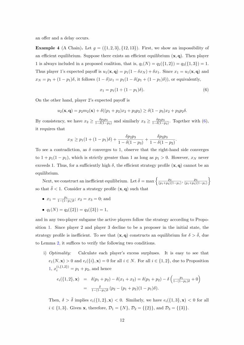
an offer and a delay occurs.

Example 4 (A Chain). Let g = ({1, 2, 3}, {12, 13}). First, we show an impossibility of

an efficient equilibrium. Suppose there exists an efficient equilibrium (x,q). Then player

1 is always included in a proposed coalition, that is, q1(N) = q2({1, 2}) = q3({1, 3}) = 1.

Thus player 1’s expected payoff is u1(x,q) = p1(1− δxN ) + δx1. Since x1 = u1(x,q) and

xN = p1 + (1− p1)δ, it follows (1− δ)x1 = p1(1− δ(p1 + (1− p1)δ)), or equivalently,

x1 = p1(1 + (1− p1)δ). (6)

On the other hand, player 2’s expected payoff is

u2(x,q) = p2m2(x) + δ((p1 + p2)x2 + p3p2) ≥ δ(1− p3)x2 + p3p2δ.

By consistency, we have x2 ≥ δp2p31−δ(1−p3) and similarly x3 ≥ δp2p3

1−δ(1−p2) . Together with (6),

it requires that

xN ≥ p1(1 + (1− p1)δ) +δp2p3

1− δ(1− p3)+

δp2p3

1− δ(1− p2).

To see a contradiction, as δ converges to 1, observe that the right-hand side converges

to 1 + p1(1 − p1), which is strictly greater than 1 as long as p1 > 0. However, xN never

exceeds 1. Thus, for a sufficiently high δ, the efficient strategy profile (x,q) cannot be an

equilibrium.

Next, we construct an inefficient equilibrium. Let δ = max{

p2(p1+p2)(1−p1) ,

p3(p1+p3)(1−p1)

}so that δ < 1. Consider a strategy profile (x,q) such that

• x1 = p11−(1−p1)δ ; x2 = x3 = 0; and

• q1(N) = q2({2}) = q3({3}) = 1,

and in any two-player subgame the active players follow the strategy according to Propo-

sition 1. Since player 2 and player 3 decline to be a proposer in the initial state, the

strategy profile is inefficient. To see that (x,q) constructs an equilibrium for δ > δ, due

to Lemma 2, it suffices to verify the following two conditions.

i) Optimality: Calculate each player’s excess surpluses. It is easy to see that

e1(N,x) > 0 and ei({i},x) = 0 for all i ∈ N . For all i ∈ {1, 2}, due to Proposition

1, x(i,{1,2})i = p1 + p2, and hence

ei({1, 2},x) = δ(p1 + p2)− δ(x1 + x2) = δ(p1 + p2)− δ(

p11−(1−p1)δ + 0

)= δ

1−(1−p1)δ (p2 − (p1 + p2)(1− p1)δ).

Then, δ > δ implies ei({1, 2},x) < 0. Similarly, we have ei({1, 3},x) < 0 for all

i ∈ {1, 3}. Given x, therefore, D1 = {N}, D2 = {{2}}, and D3 = {{3}}.

12

ii) Consistency: Compute each player’s expected payoff:

• u1(x,q) = p1e(N,x) + δx1 = p1(1− δx1) + δx1 = p1 + (1− p1)δ(

p11−(1−p1)δ

)= p1

1−(1−p1)δ

• u2(x,q) = p2e({2},x) + δx2 = p2 · 0 + δ · 0 = 0

• u3(x,q) = p3e({3},x) + δx3 = p3 · 0 + δ · 0 = 0.

Therefore, ui(x,q) = xi for all i ∈ N .

Even if there are multiple dominating players, as see (b) in Figure 2, they can generate

an additional advantage by forming a coalition with other dominating players and splitting

non-dominating players into two isolated groups. In the next example, we construct an

equilibrium in a chordal network in which there are two dominating players.

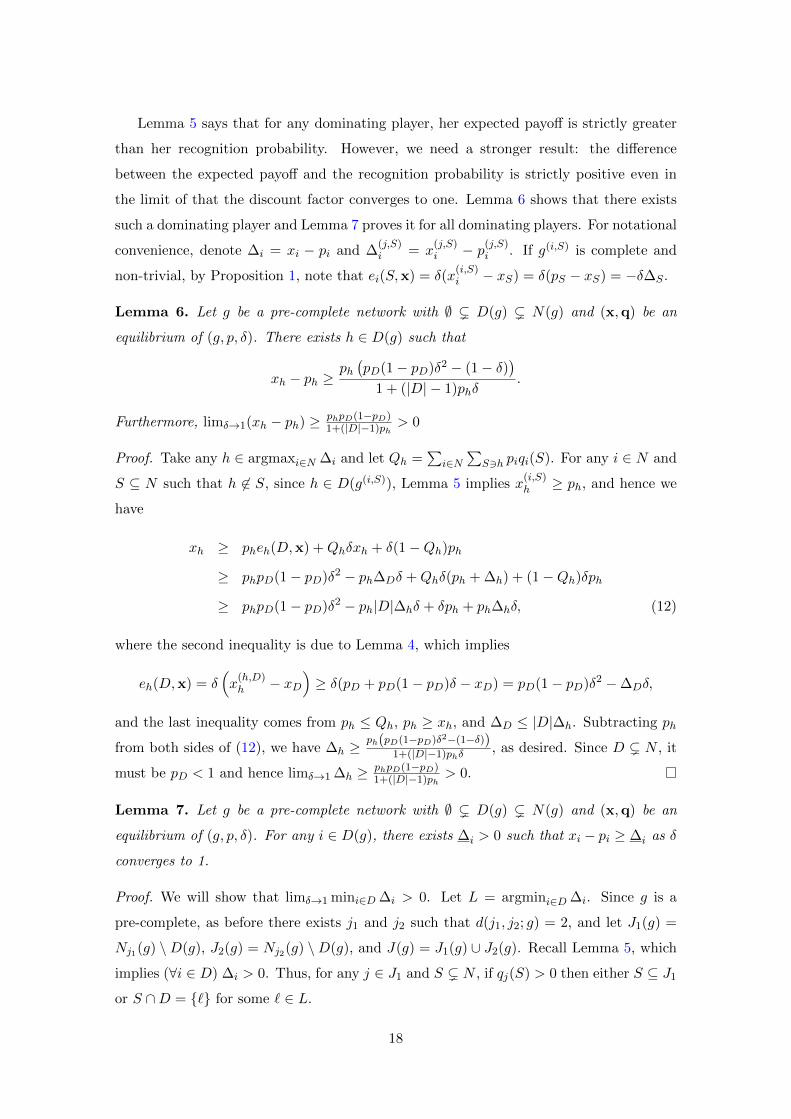
Example 5 (A Chordal Network). Let g = ({1, 2, 3, 4}, {12, 23, 34, 41, 13}) and p =

(14 ,

14 ,

14 ,

14). Suppose δ > δ ≈ 0.91.12 We construct an equilibrium (x,q) such that

• x1 = x3 = (6−δ)δ4(4−δ)(2−δ) ; x2 = x4 = (6−6δ+δ2)δ

4(4−δ)(2−δ) ;

• q1({1, 3}) = q3({1, 3}) = 1; q2({1, 2}) = q2({2, 3}) = q4({1, 4}) = q4({3, 4}) = 12 .

In any subgame in which the number of active players is less than or equal to three,

they follows the equilibrium strategies according to Proposition 1 and Example 4. Note

that the equilibrium welfare is xN = δ(3−δ)2(2−δ) . The equilibrium payoff vector converges to(

512 ,

112 ,

512 ,

112

)as δ → 1. Now we verify the equilibrium conditions.

i) Odd Players’ Optimality: Since δ > 34 , Example 4 implies that x

(1,{1,3})1 =

p1+p31−(1−p1−p3)δ = 1

2−δ and x(1,{1,3})1 = x

(1,{1,3})4 = 0. Given x, calculate player 1’s

excess surpluses:

• e1({1, 2},x) = δx(1,{1,2})1 − δ(x1 + x2) = δ(1−δ)(4−δ)

4(2−δ)

• e1({1, 3},x) = δx(1,{1,3})1 − δ(x1 + x3) = δ(8−8δ+δ2)

2(2−δ)(4−δ)

• e1({1, 2, 4},x) = δx(1,{1,2,4})1 − δ(x1 + x2 + x4) = δ(6−6δ+δ2)

2(4−δ)

• e1(N,x) = 1− δxN = (1−δ)(4+2δ−δ2)2(2−δ)

Given e1(S,x) for all S ⊆ N1, it is routine to see that δ > δ implies D1(x) =

{{1, 3}}. Similarly, we also have D3(x) = {{1, 3}}.

ii) Even Players’ Optimality: For any {2} ( S ⊆ N2, player 2’s S-formation induces

a complete network. Thus, given x, one can compute player 2’s excess surpluses:

12Note that δ is a solution to δ(8− 8δ + δ2) = (4− δ)(1− δ)(4 + 2δ − δ2).

13

• e2({1, 2},x) = e2({2, 3},x) = δx(2,{1,2})2 − δ(x1 + x2) = δ(1−δ)(4−δ)

4(2−δ)

• e({1, 2, 3},x) = δx(2,{1,2,3})2 − δ(x1 + x2 + x3) = δ(24−36δ+11δ2−δ3)

4(2−δ)(4−δ)

Observe that e2({1, 2},x) = e2({2, 3},x) > 0 for all δ; while e({1, 2, 3},x) is strictly

negative if δ > δ. Thus, for any δ > δ, we have D2(x) = {{1, 2}, {2, 3}} and

similarly D4(x) = {{1, 4}, {3, 4}}.

iii) Consistency: Given (x,q), compute each players’ expected payoffs:

• u1(x,q) = p1e({1, 3},x) + δ[(p1 + p3 + 1

2(p2 + p4))x1 + 1

2(p2 + p4)p1

]= 1

4 ·δ(8−8δ+δ2)2(2−δ)(4−δ) + δ

[34 ·

(6−δ)δ4(4−δ)(2−δ) + 1

2 ·18

]= (6−δ)δ

4(4−δ)(2−δ) = x1

,

• u2(x,q) = p2e({1, 2},x) + δ [p2x2 + p4p2 + (p1 + p3) · 0]

= 14 ·

δ(1−δ)(4−δ)4(2−δ) + δ

[14 ·

(6−6δ+δ2)δ4(4−δ)(2−δ) + 1

4 ·14

]= (6−6δ+δ2)δ

4(4−δ)(2−δ) = x2

,

and similarly u3(x,q) = x3 and u4(x,q) = x4, and hence consistency holds.

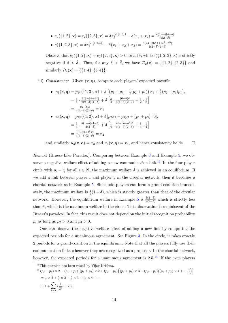
Remark (Braess-Like Paradox). Comparing between Example 3 and Example 5, we ob-

serve a negative welfare effect of adding a new communication link.13 In the four-player

circle with pi = 14 for all i ∈ N , the maximum welfare δ is achieved in an equilibrium. If

we add a link between player 1 and player 3 in the circular network, then it becomes a

chordal network as in Example 5. Since odd players can form a grand-coalition immedi-

ately, the maximum welfare is 12(1 + δ), which is strictly greater than that of the circular

network. However, the equilibrium welfare in Example 5 is δ(3−δ)2(2−δ) which is strictly less

than δ, which is the maximum welfare in the circle. This observation is reminiscent of the

Braess’s paradox. In fact, this result does not depend on the initial recognition probability

p, as long as p2 > 0 and p4 > 0.

One can observe the negative welfare effect of adding a new link by computing the

expected periods for a unanimous agreement. See Figure 3. In the circle, it takes exactly

2 periods for a grand-coalition in the equilibrium. Note that all the players fully use their

communication links whenever they are recognized as a proposer. In the chordal network,

however, the expected periods for a unanimous agreement is 2.5.14 If the even players

13This question has been raised by Vijay Krishna.14 (p2 + p4)× 2 + (p1 + p3)

[(p1 + p3)× 2 + (p2 + p4)

((p1 + p3)× 3 + (p2 + p4)

((p1 + p3)× 4 + · · ·

))]= 1

2× 2 + 1

4× 2 + 1

8× 3 + 1

16× 4 + · · ·

= 1 +

∞∑k=2

k1

2k= 2.5.

14

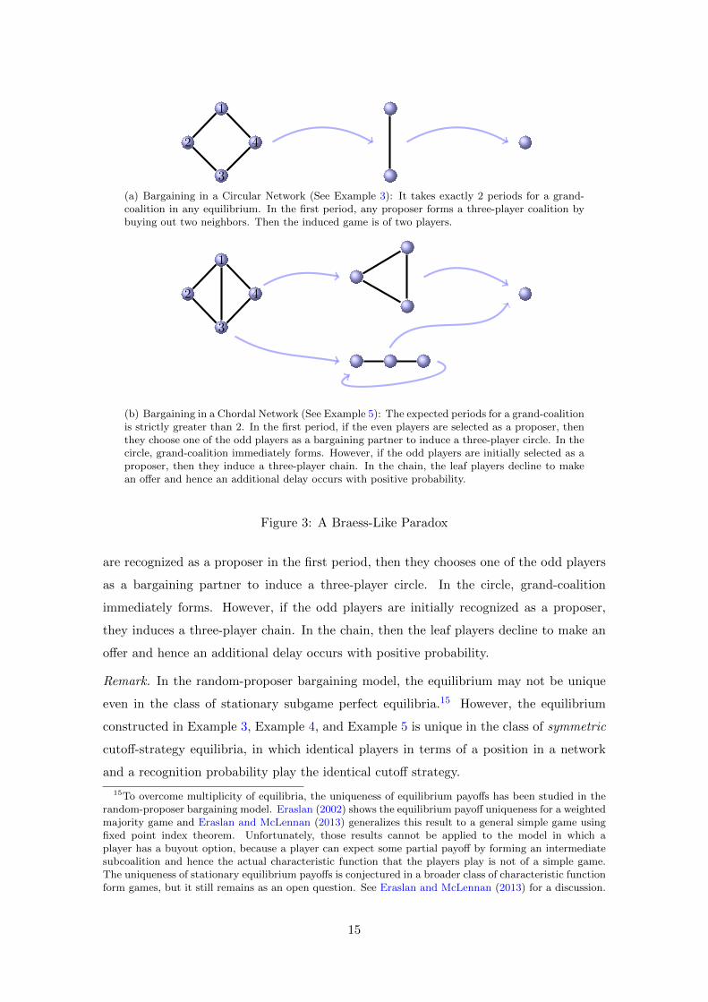
1

2

3

4

(a) Bargaining in a Circular Network (See Example 3): It takes exactly 2 periods for a grand-coalition in any equilibrium. In the first period, any proposer forms a three-player coalition bybuying out two neighbors. Then the induced game is of two players.

1

2

3

4

(b) Bargaining in a Chordal Network (See Example 5): The expected periods for a grand-coalitionis strictly greater than 2. In the first period, if the even players are selected as a proposer, thenthey choose one of the odd players as a bargaining partner to induce a three-player circle. In thecircle, grand-coalition immediately forms. However, if the odd players are initially selected as aproposer, then they induce a three-player chain. In the chain, the leaf players decline to makean offer and hence an additional delay occurs with positive probability.

Figure 3: A Braess-Like Paradox

are recognized as a proposer in the first period, then they chooses one of the odd players

as a bargaining partner to induce a three-player circle. In the circle, grand-coalition

immediately forms. However, if the odd players are initially recognized as a proposer,

they induces a three-player chain. In the chain, then the leaf players decline to make an

offer and hence an additional delay occurs with positive probability.

Remark. In the random-proposer bargaining model, the equilibrium may not be unique

even in the class of stationary subgame perfect equilibria.15 However, the equilibrium

constructed in Example 3, Example 4, and Example 5 is unique in the class of symmetric

cutoff-strategy equilibria, in which identical players in terms of a position in a network

and a recognition probability play the identical cutoff strategy.

15To overcome multiplicity of equilibria, the uniqueness of equilibrium payoffs has been studied in therandom-proposer bargaining model. Eraslan (2002) shows the equilibrium payoff uniqueness for a weightedmajority game and Eraslan and McLennan (2013) generalizes this result to a general simple game usingfixed point index theorem. Unfortunately, those results cannot be applied to the model in which aplayer has a buyout option, because a player can expect some partial payoff by forming an intermediatesubcoalition and hence the actual characteristic function that the players play is not of a simple game.The uniqueness of stationary equilibrium payoffs is conjectured in a broader class of characteristic functionform games, but it still remains as an open question. See Eraslan and McLennan (2013) for a discussion.

15

Now, we are ready to prove Proposition 3 in a case of D(g) 6= ∅. Since g is a pre-

complete, note that there exists j1 and j2 such that d(j1, j2; g) = 2. Let J1(g) = Nj1(g) \

D(g), J2(g) = Nj2(g) \D(g), and J(g) = J1(g)∪ J2(g). Lemma 4 provides a lower bound

of the unique dominating player’s expected payoff.

Lemma 4. Let g be a pre-complete network with D(g) = {i}. If (x,q) is an equilibrium

of Γ = (g, p, δ), then

xi ≥ pi + pi(1− pi)δ. (7)

Proof. Step 1: Consider a three-person chain, that is, J1 = {j1} and J2 = {j2}. Since

x(j1,J1)i = x

(j2,J2)i = xi and uN (x,q) ≤ u(Γ) = pi + δ(1− pi), player i’s expected payoff is

xi ≥ piei(N,x) +∑k∈N

pk∑S3i

qk(S)δxi + δ∑k∈N

pk∑S 63i

qk(S)xi

≥ pi(1− δ(pi + δ(1− pi))) + δxi.

Rearranging the terms, we have the desired result.

Step 2: As an induction hypothesis, assume that for any pre-complete network g′ with

D(g′) = {i}, ≤ |J1(g′)| ≤ a, and 1 ≤ |J2(g′)| ≤ b, x′i ≥ p′i + p′i(1− p′i)δ. Now we consider

a pre-complete network g with D(g) = {i}, |J1(g)| = a, and |J1(g)| = b + 1. Player i’s

expected payoff is

xi ≥ piei(N,x) +∑k∈N

pk∑S3i

qk(S)δxi + δ∑k∈N

pk∑S 63i

qk(S)x(k,S)i . (8)

For any k ∈ N and S ⊆ N such that i 6∈ S, the induction hypothesis implies x(k,S)i ≥

pi+pi(1−pi)δ. Suppose by way of contradiction that pi+pi(1−pi)δ > xi. Then, (8) can

be written as xi ≥ pi (1− δ(pi + δ(1− pi))) + δxi, or equivalently, xi > pi + pi(1 − pi)δ,

which yields a contradiction. Similarly, induction argument completes the proof.

Proof of Proposition 3 (Case 1: D(g) 6= ∅)

Take any j ∈ J1. Since (x,q) is efficient, we have (∀j′ ∈ J2)∑

S∈Cj′qj′(S) = 1 and

(∀i ∈ D ∪ J1)∑

j∈S⊆N qi(S) = 1. Thus, player j’s payoff is

uj(x,q) = pjmj(x) + δ(pD + pJ1)xj + δ∑j′∈J2

pj′∑S⊆N

qj′(S)x(j′,S)j

≥ δ(pD + pJ1)xj + δpJ2pj ,

which implies that xj ≥pjpJ2δ

1−(1−pJ2 )δ . Summing j over J1, we have xJ1 ≥pJ1pJ2δ

1−(1−pJ2 )δ .

Similarly for J2, we have xJ2 ≥pJ1pJ2δ

1−(1−pJ1 )δ , and hence

xJ = xJ1 + xJ2 ≥ pJ1pJ2δ(

1

1− (1− pJ1)δ+

1

1− (1− pJ2)δ

)(9)

16

Now take any i ∈ D. Player i’s optimality implies ei(N,x) ≥ ei(D,x), or equivalently,

1 − δxN ≥ δx(i,D)i − δxD. Since g(i,D) has a single dominating player, Lemma 4 implies

x(i,D)i ≥ pD + pD(1− pD)δ and it follows that

1− pDδ(1 + δ − pDδ) ≥ δxJ (10)

By (9) and (10), we have

1− pDδ(1 + δ − pDδ) ≥ pJ1pJ2δ2

(1

1− (1− pJ1)δ+

1

1− (1− pJ2)δ

). (11)

As δ → 1, the right hand side of (11) converges to pJ ; while the left hand side converges

to p2J . Since pJ < 1, there exists δ < 1 such that the inequality (11) yields a contradiction

for δ > δ.

3.2.2 Case 2: No Dominating Player

Now we consider a network without a dominating player. See (c) in Figure 2 for instance.

Even in a case of that there is no dominating player, we will show that some players can be

a dominating player in the induced network by buying out only a part of their neighbors.

Before proving this, some lemmas are presented. First, whenever there is a dominating

player in an incomplete network, Lemma 5, Lemma 6, and Lemma 7 show dominating

players have some additional bargaining power compared to other non-dominating players.

In a network without a dominating player, Lemma 8 shows that each player’s payoff should

be strictly less than her recognition probability under any efficient equilibrium. For any

non-circular pre-complete network without a dominating player, Lemma 9 finds a player

who can be a dominating player avoiding a complete network. Combining those lemmas,

therefore, when an efficient equilibrium is assumed, at least one player can be strictly

better off by strategically delaying a unanimous agreement, which is a contradiction in

turn.

Lemma 5. Let g be a pre-complete network with ∅ ( D(g) ( N(g) and (x,q) be an

equilibrium of (g, p, δ) with δ < 1. If i ∈ D(g) then xi > pi.

Proof. If |N(g)| = 3, due to Lemma 4, then xi ≥ pi + pi(1− pi)δ > pi for any i ∈ D. As

an induction hypothesis, suppose the statement is true for any g′ with |N(g′)| < n. Now

consider g with |N(g)| = n. Take any i ∈ D(g). For any k ∈ N and any S such that

i 6∈ S, if g(k,S) is complete then x(k,S)i = pi; and if g(k,S) is incomplete then x

(k,S)i > pi by

the induction hypothesis. Thus, letting Qi =∑

k∈N pk(∑

S3i qi(S) + qk({k})), we have

xi ≥ pi(1− δxN ) +Qiδxi + δ(1−Qi)pi, and hence xi ≥ pi + δ(1−δ)1−δQi pi > pi.

17

Lemma 5 says that for any dominating player, her expected payoff is strictly greater

than her recognition probability. However, we need a stronger result: the difference

between the expected payoff and the recognition probability is strictly positive even in

the limit of that the discount factor converges to one. Lemma 6 shows that there exists

such a dominating player and Lemma 7 proves it for all dominating players. For notational

convenience, denote ∆i = xi − pi and ∆(j,S)i = x

(j,S)i − p(j,S)

i . If g(i,S) is complete and

non-trivial, by Proposition 1, note that ei(S,x) = δ(x(i,S)i − xS) = δ(pS − xS) = −δ∆S .

Lemma 6. Let g be a pre-complete network with ∅ ( D(g) ( N(g) and (x,q) be an

equilibrium of (g, p, δ). There exists h ∈ D(g) such that

xh − ph ≥ph(pD(1− pD)δ2 − (1− δ)

)1 + (|D| − 1)phδ

.

Furthermore, limδ→1(xh − ph) ≥ phpD(1−pD)1+(|D|−1)ph

> 0

Proof. Take any h ∈ argmaxi∈N ∆i and let Qh =∑

i∈N∑

S3h piqi(S). For any i ∈ N and

S ⊆ N such that h 6∈ S, since h ∈ D(g(i,S)), Lemma 5 implies x(i,S)h ≥ ph, and hence we

have

xh ≥ pheh(D,x) +Qhδxh + δ(1−Qh)ph

≥ phpD(1− pD)δ2 − ph∆Dδ +Qhδ(ph + ∆h) + (1−Qh)δph

≥ phpD(1− pD)δ2 − ph|D|∆hδ + δph + ph∆hδ, (12)

where the second inequality is due to Lemma 4, which implies

eh(D,x) = δ(x

(h,D)h − xD

)≥ δ(pD + pD(1− pD)δ − xD) = pD(1− pD)δ2 −∆Dδ,

and the last inequality comes from ph ≤ Qh, ph ≥ xh, and ∆D ≤ |D|∆h. Subtracting ph

from both sides of (12), we have ∆h ≥ph(pD(1−pD)δ2−(1−δ))

1+(|D|−1)phδ, as desired. Since D ( N , it

must be pD < 1 and hence limδ→1 ∆h ≥ phpD(1−pD)1+(|D|−1)ph

> 0.

Lemma 7. Let g be a pre-complete network with ∅ ( D(g) ( N(g) and (x,q) be an

equilibrium of (g, p, δ). For any i ∈ D(g), there exists ∆i > 0 such that xi − pi ≥ ∆i as δ

converges to 1.

Proof. We will show that limδ→1 mini∈D ∆i > 0. Let L = argmini∈D ∆i. Since g is a

pre-complete, as before there exists j1 and j2 such that d(j1, j2; g) = 2, and let J1(g) =

Nj1(g) \D(g), J2(g) = Nj2(g) \D(g), and J(g) = J1(g) ∪ J2(g). Recall Lemma 5, which

implies (∀i ∈ D) ∆i > 0. Thus, for any j ∈ J1 and S ( N , if qj(S) > 0 then either S ⊆ J1

or S ∩D = {`} for some ` ∈ L.

18

Case 1: Suppose |J1| = |J2| = 1. Then, for each j ∈ J , qj({j}) +∑

`∈L qj({j, `}) = 1,

and hence there exists ` ∈ L such that∑

j∈J pj (qj({j}) + qj({j, `})) ≥ pJ|L| . Let Q` =∑

j∈J pj (qj({j}) + qj({j, `}))+∑

i∈D∑

S3` piqi(S), thenQ` ≥ pJ|L|+p`. Since x` ≥ p`e`(J∪

{`},x) +Q`δx` + (1−Q`)δp`, it follows

∆` ≥ δp`(∆` + ∆J) + δ

(pJ|L|

+ p`

)∆` − (1− δ)p`,

which implies ∆` ≥ −δp`∆J−(1−δ)p`1−δ pJ|L|

. Since xN−pN = ∆N < 0, we have −∆J ≥ ∆D ≥ ∆h.

Thus, by Lemma 6, we have the desired result,

limδ→1

∆` ≥ −|L|p`|L| − pJ

∆J ≥|L|p`|L| − pJ

∆h ≥p`phpD(1− pD)|L|

(|L| − pJ)(1 + (|D| − 1)ph)> 0.

Case 2: As an induction hypothesis, for any pre-complete network g′ with ∅ ( D(g′) (

N(g′) and 1 ≤ |J1(g′)| ≤ a and 1 ≤ |J2(g′)| ≤ b and any equilibrium (x′,q′) of (g′, p′, δ),

assume that limδ→1 mini∈D(g′)(x′i − p′i) > 0. Now we consider a pre-complete network

g with ∅ ( D(g) ( N(g) and |J1(g)| = a and |J2(g)| = b + 1. Due to the induction

hypothesis, there exists ∆′` > 0 such that ∆′` ≥ limδ→1(x(j,J ′)` − p`) for all α ∈ {1, 2},

j ∈ Jα, and J ′ ⊆ Jα. Then, we have

x` ≥ p`e`(J ∪ {`},x) +

p` +∑

α∈{1,2}

∑j∈Jα

pj (qj({j}) + qj(Jα ∪ {`}))

δ(p` + ∆`)

+

∑α∈{1,2}

∑j∈Jα

∑J ′⊆Jα

pjqj(J′)

δ(p` + ∆′`) + pD\{`}δp`. (13)

If limδ→1 ∆` ≥ ∆′`, then there is nothing to prove. Suppose that limδ→1 ∆` ≤ ∆′`. As

δ → 1, then (13) yields x` ≥ −p`δ∆J + δp` + (1 − pD)δ∆`, or equivalently, (1 − (1 −

pD)δ)∆` ≥ −δp`∆J − (1− δ)p`. Take any h ∈ argmaxi∈D ∆i. Since −∆J > ∆D > ∆h, it

follows that

(1− (1− pD)δ)∆` > δp`∆h − (1− δ)p`.

By Lemma 5, we have the desired result, limδ→1 ∆` ≥ p`ph(1−pD)1+(|D|−1)ph

> 0.

Lemma 8. Let g be a pre-complete network with D(g) = ∅. If (x,q) is an efficient

equilibrium of Γ = (g, p, δ), then for all i ∈ N , xi = δpi.

Proof. Since g is pre-complete and (x,q) is efficient, for all j ∈ N , qj(S) > 0 implies g(j,S)

is complete. Thus, each player i can expect pi in the next period by rejecting any offer.

Suppose player i gets an offer with yi < δ2pi. By rejecting yi, i can be strictly better

since the stationary strategy profile guarantees δpi in the next period. Hence, xi ≥ δpi

for all i ∈ N . If there exists i ∈ N such that xi > δpi, then it must be xN > δpN = δ,

which is infeasible.

19

Lemma 9. Let g be a pre-complete non-circular network with D(g) = ∅. There exist

i, j ∈ N(g) such that i ∈ D(g(i,{i,j})) ( N(g(i,{i,j})).

Proof. Since g is pre-complete non-circular, its complete covering number is 2. Let M

be a minimal complete cover of g. Since D(g) = ∅, M must be disjoint. Given i ∈ N ,

then let Mi ∈ M such that i ∈ Mi. Since D(g) = ∅, for all k ∈ N , there exists at

least one k′ ∈ M ck such that kk′ 6∈ E(g), that is, it must be |M c

k \ Nk(g)| ≥ 1. We will

show that there exists i ∈ N and j ∈ M ci such that i ∈ D(g(i,{i,j})) ( N(g(i,{i,j})), by

constructing such a pair of i and j in the following two cases. First, suppose there exists

k ∈ N such that |M ck \ Nk(g)| ≥ 2. Take i ∈ M c

k \ Nk(g) and j ∈ M ci with ij ∈ E(g).

Take i′ ∈ M ck \ Nk(g) with i′ 6= i. Since g|Mi

and g|Mci

are complete, i ∈ D(g(i,{i,j})).

Since d(k, i′; g) = d(k, i′; g(i,{i,j})) = 2, k 6∈ N(g(i,{i,j})), as desired. Second, suppose, for

all k ∈ N , |M ck \ Nk(g)| = 1. Take any i ∈ N and j ∈ M c

i such that ij ∈ E(g). Take

k ∈ Mi \ {i} and k′ ∈ M ci such that d(k, k′; g) = 2. Again we have i ∈ D(g(i,{i,j})) and

d(k, k′; g) = d(k, k′; g(i,{i,j})) = 2, as desired.

Proof of Proposition 3 (Case 2: D(g) = ∅)

Suppose (x,q) is an efficient equilibrium. Due to Lemma 8, for all i ∈ N and all S ∈ Ci,

ei(S,x) = δ(x

(i,S)i − xS

)= δ (pS − δpS) = δ(1− δ)pS ,

which converges to 0 as δ → 1. By Lemma 9, there exists i, j ∈ N(g) such that i ∈

D(g(i,{i,j})) and {i, j} 6∈ Ci. Due to Lemma 7, there exists ∆i such that x(i,{i,j})i −p(i,{i,j})

i ≥

∆i. By Lemma 8, then we have

ei({i, j},x) = δ(x

(i,{i,j})i − (xi + xj)

)≥ δ

((p

(i,{i,j})i + ∆i − δ(pi + pj)

)= δ∆i + δ(1− δ)(pi + pj).

As δ → 1, note that ei({i, j},x) ≥ ∆i > 0. Thus for a sufficiently high δ, ei({i, j},x) >

ei(S,x) for all S ∈ Ci, which contradicts to optimality of player i.

3.3 The Necessary Condition : Incomplete Networks

We have considered pre-complete non-circular networks. To complete the necessary condi-

tion, we have to allow any incomplete non-circular network. Proposition 4 implies that for

any game with an incomplete non-circular network, if the players play efficient strategies,

then a pre-complete non-circular network must be induced with positive probability.

20

Proposition 4. Let g be an incomplete network. For any efficient strategy profile (x,q),

there exists π ∈ Πx,q(g) such that gπ is a pre-complete network. In addition, if g is a non-

circular network, then there exists π ∈ Πx,q(g) such that gπ is a pre-complete non-circular

network.

Proof. Suppose that g is neither pre-complete nor complete. Now we construct a sequence

of coalition formations which is consistent with (x,q) and the sequence induces a pre-

complete network. Take i∗ ∈ argmaxi∈N(g) degi(g). Let I(g) = {i ∈ N(g) | Ci(g) = ∅}.

Let g1 = g and take i1 ∈ argmaxi∈I(g1) d(i, i∗; g1). Pick any S1 such that qi1(S1) > 0.

Let g2 = g(i1,S1). Similarly, pick i2 ∈ argmaxi∈I(g2) d(i, i∗; g2). Pick any S2 such that

qi2(S2) > 0. Since (x,q) is efficient, |S1| ≥ 2, |S2| ≥ 2, and so on; and I(g1) ) I(g2) ) · · · .

Thus, one can repeat this process until I(gT ) = ∅, after which gT is a pre-complete

network. This proves the first part. In addition, assume that g is not circular. If g is a

tree, then any induced network cannot be circular and hence gT is not circular. If g has

a cycle but not a circular network, then degi∗(g) = degi∗(gT ) ≥ 3, and hence gT cannot

be circular.

4 Non-transferability of Recognition Probabilities

We have assumed that the initial recognition probabilities are transferable. That is, when

they trade their communication links, they also trade their chances of being a proposer

as well. In some other environment, however, players cannot trade their recognition

probabilities. With non-transferable recognition probabilities, instead of (1), we define

the recognition probabilities in any state π in the following way:

pπi =

pi∑

k∈Nπ pkif i ∈ Nπ

0 otherwise.(14)

With non-transferable recognition probabilities, obtaining an efficient equilibrium is

impossible even in circular networks.

Theorem 2. With non-transferable recognition probabilities, an efficient equilibrium

exists for all discount factors if and only if the underlying network is complete.

Before proving the theorem, we construct an inefficient equilibrium in a four-player

circular network as an example.

Example 6 (A Circular Network with Non-Transferable Recognition Probabilities).

Let g = ({1, 2, 3, 4}, {12, 23, 34, 14}) and p =(

14 ,

14 ,

14 ,

14

). If δ > 2

3 , then there exists a

cutoff strategy equilibrium (x,q) such that

21

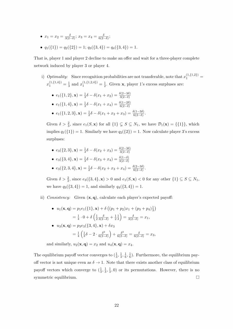
• x1 = x2 = δ3(2−δ) ; x3 = x4 = δ

6(2−δ) ;

• q1({1}) = q2({2}) = 1; q3({3, 4}) = q4({3, 4}) = 1.

That is, player 1 and player 2 decline to make an offer and wait for a three-player complete

network induced by player 3 or player 4.

i) Optimality: Since recognition probabilities are not transferable, note that x(1,{1,2})1 =

x(1,{1,4})1 = 1

3 and x(1,{1,2,4})1 = 1

2 . Given x, player 1’s excess surpluses are:

• e1({1, 2},x) = 13δ − δ(x1 + x2) = δ(2−3δ)

3(2−δ)

• e1({1, 4},x) = 13δ − δ(x1 + x4) = δ(1−2δ)

6(2−δ)

• e1({1, 2, 3},x) = 12δ − δ(x1 + x2 + x3) = δ(1−3δ)

6(2−δ) .

Given δ > 23 , since e1(S,x) for all {1} ( S ⊆ N1, we have D1(x) = {{1}}, which

implies q1({1}) = 1. Similarly we have q2({2}) = 1. Now calculate player 3’s excess

surpluses:

• e3({2, 3},x) = 13δ − δ(x2 + x3) = δ(2−3δ)

3(2−δ)

• e3({3, 4},x) = 13δ − δ(x3 + x4) = δ(1−δ)

3(2−δ)

• e3({2, 3, 4},x) = 12δ − δ(x2 + x3 + x4) = δ(2−3δ)

6(2−δ) .

Given δ > 23 , since e3({3, 4},x) > 0 and e1(S,x) < 0 for any other {1} ⊆ S ⊆ N1,

we have q3({3, 4}) = 1, and similarly q4({3, 4}) = 1.

ii) Consistency: Given (x,q), calculate each player’s expected payoff:

• u1(x,q) = p1e1({1},x) + δ((p1 + p2)x1 + (p3 + p4)1

3

)= 1

4 · 0 + δ(

12

δ3(2−δ) + 1

213

)= δ

3(2−δ) = x1,

• u3(x,q) = p3e3({3, 4},x) + δx3

= 14

(13δ − 2 · δ2

6(2−δ)

)+ δ2

6(2−δ) = δ6(2−δ) = x3,

and similarly, u2(x,q) = x2 and u4(x,q) = x4.

The equilibrium payoff vector converges to (13 ,

13 ,

16 ,

16). Furthermore, the equilibrium pay-

off vector is not unique even as δ → 1. Note that there exists another class of equilibrium

payoff vectors which converge to (13 ,

13 ,

13 , 0) or its permutations. However, there is no

symmetric equilibrium.

22

Now we prove Theorem 2. Since Proposition 1 still holds with non-transferable recog-

nition probabilities, this directly proves the sufficient condition. Proposition 5 shows that

an efficient equilibrium is impossible for any pre-complete network. Due to the first part

of Proposition 4, then, the necessary condition is proved for any incomplete network.

Proposition 5. Suppose that recognition probabilities are not transferable. Let g be a

pre-complete. For any p, there exists δ < 1 such that for all δ > δ, any efficient strategy

profile (x,q) cannot be an equilibrium in Γ = (g, p, δ).

Proof. Since g is incomplete, N(g) \ D(g) 6= ∅. After renaming, let N(g) \ D(g) =

{1, · · · , L}. For each 1 ≤ ` ≤ L, take any S` such that q`(S`) > 0. Since (x,q) is efficient,

S` ∈ C`. Due to Proposition 1, we have x(`,S`)` = p

(`,S`)` . Since non-transferable recognition

probabilities are assumed, we have

x(`,S`)` = p

(`,S`)` =

p`∑j∈N\S` pj + p`

=∑j∈S`

pj −

(∑j∈N\S` pj

)(∑j∈S`\{`} pj

)∑

j∈N\S` pj + p`. (15)

In addition, since S`-formation is optimal for each `, it must be e`(S`,x) ≥ e`({`},x) = 0,

or equivalently,∑

j∈S` xj ≤ x(`,S`)` . Summing this over ` and plugging (15), we have

L∑`=1

∑j∈S`

xj ≤L∑`=1

∑j∈S`

pj − ρ, (16)

where

ρ =L∑`=1

(∑j∈N\S` pj

)(∑j∈S`\{`} pj

)∑

j∈N\S` pj + p`.

Note that ρ is strictly positive and does not depend on δ.

On the other hand, for any k’s S-formation such that qk(S) > 0 and any j 6∈ S, it must

be x(k,S)j = p

(k,S)j =

pj∑`∈N\S pk+pk

> pj . Then, for each j ∈ N , j’s continuation payoff is

uj(x,q) = pjmj(x) + δ∑k∈N

pk

∑S3j

qk(S)xj +∑S 63j

qk(S)x(k,S)j

≥ δ

∑k∈N

pk

∑S3j

qk(S)xj +∑S 63j

qk(S)p(k,S)j

> Qjxj + (1−Qj)pj .

where Qj =∑

k∈N pk∑

S3j qk(S). By the consistency condition, it follows that

xj >(1−Qj)δpj

1−Qjδ(17)

23

Combining (16) and (17), we have,

δ

L∑`=1

∑j∈S`

(1−Qj)pj1−Qjδ

+ ρ <

L∑`=1

∑j∈S`

pj . (18)

As δ → 1, δ∑L

`=1

∑j∈S`

(1−Qj)pj1−Qjδ converges to

∑L`=1

∑j∈S` pj . However, this contradicts

to the fact that ρ > 0 is fixed. Thus, there exists δ < 1 such that for all δ > δ, the

inequality (18) is violated.

Remark. In network-restricted unanimity games, welfare can be improved by allowing for

players to trade their recognition probabilities. If the recognition probabilities are not

transferable, a proposer has less incentive to form a coalition. In general characteristic

function form games, however, the effect of transferability of recognition probabilities

on welfare may be negative. For instance, when there exists a veto player, non-veto

players may form a union, to be a new veto coalition, as a transitional state, rather than

immediately forming an efficient coalition. If the recognition probabilities are transferable,

then they have stronger incentive to form transitional inefficient coalitions. Thus, for a

non-unanimity game, banning players from trading recognition probabilities may improve

welfare. See Lee (2014) for details.

References

Abreu, D. and M. Manea (2012a): “Bargaining and efficiency in networks,” Journal

of Economic Theory, 147, 43–70.

——— (2012b): “Markov equilibria in a model of bargaining in networks,” Games and

Economic Behavior, 75, 1–16.

Aumann, R. J. and J. H. Dreze (1974): “Cooperative games with coalition structures,”

International Journal of game theory, 3, 217–237.

Braess, D. (1968): “Uber ein Paradoxon aus der Verkehrsplanung,” Un-

ternehmensforschung, 12, 258–268.

Braess, D., A. Nagurney, and T. Wakolbinger (2005): “On a paradox of traffic

planning,” Transportation science, 39, 446–450.

Eraslan, H. (2002): “Uniqueness of stationary equilibrium payoffs in the Baron–

Ferejohn model,” Journal of Economic Theory, 103, 11–30.

24

Eraslan, H. and A. McLennan (2013): “Uniqueness of stationary equilibrium payoffs

in coalitional bargaining,” Journal of Economic Theory, 148, 2195–2222.

Gul, F. (1989): “Bargaining foundations of Shapley value,” Econometrica: Journal of

the Econometric Society, 81–95.

Hart, S. and A. Mas-Colell (1996): “Bargaining and value,” Econometrica: Journal

of the Econometric Society, 357–380.

Lee, J. (2014): “Bargaining and Buyout,” working paper, available at https://sites.

google.com/site/joosungecon/Buyout_posting.pdf.

Manea, M. (2011a): “Bargaining in dynamic markets with multiple populations,” work-

ing paper.

——— (2011b): “Bargaining in stationary networks,” The American Economic Review,

101, 2042–2080.

Myerson, R. B. (1977): “Graphs and cooperation in games,” Mathematics of operations

research, 2, 225–229.

Nguyen, T. (2012): “Coalitional bargaining in networks.” in ACM Conference on Elec-

tronic Commerce, vol. 772.

Roughgarden, T. (2005): Selfish routing and the price of anarchy, MIT press.

Appendix

Proof of i) in Proposition 1.

Case 1: |N(g)| = 2. Let N(g) = {i, j} and p = (pi, pj) with pi + pj = 1. We show that

a cutoff strategy profile ({p1, p2}, {qi(N) = 1, qj(N) = 1}) is an equilibrium by verifying

player i has no profitable deviation strategy given player j’s cutoff strategy. Note that

player i’s expected payoff from following her cutoff strategy is pi(1− δpj) + pj(δpi) = pi.

First, consider player i’s proposal strategy. Either making an offer with yj < δpj or

declining to make an offer yields an expected payoff δpi. Making an offer with yj > δpj is

not profitable since the offer yj = δpj will be accepted. Thus, player i cannot be better off

by deviating from the given proposal strategy. Next, consider player i’s response strategy.

By rejecting any offer, player i expects the payoff pi in the next period. Thus, rejecting

any offer with yi < δpi is optimal. It is clear that accepting any offer with yi ≥ δpi is

25

optimal. Therefore, player i has no profitable deviation strategy given player j’s cutoff

strategy.

Case 2: |N(g)| > 2. Suppose that, for any game (g′, p′, δ) with |N(g′)| < |N(g)|, (p′, q′)

is an equilibrium, where p′ = {{p′πi }i∈Nπ}π∈Π(g′) and q′ = {{qπi }i∈Nπ}π∈Π(g′). Note that,

in such an equilibrium, for each i ∈ N(g′), player i’s expected payoff is p′i. We show that

a cutoff strategy profile σ = (p, q) is an equilibrium for (g, p, δ) by verifying player i has

no profitable deviation strategy given other players cutoff strategies. Recall that if player

i follows the cutoff strategy, then her expected payoff is pi(1 − δ) + δpi = pi. Since all

the other players except for i are supposed to play stationary strategies, it is enough to

consider the proposal strategy and the response strategy of player i separately.

• Proposal strategy: Consider player i’s proposal strategy qi such that qi(S) > 0

for some S ( N instead of qi. By forming S ( N , player i expects p(i,S)i in

the subsequent game, because (g(i,S), p(i,S), δ) is a less-than-n-player game with a

complete network. In order for S to form, it must be yj ≥ δpj for all j ∈ S \ {i}.

Note also that p(i,S)i ≤ pS .16 Thus, player i’s proposal gain from S-formation is

δp(i,S)i −

∑j∈S\{i}

yj ≤ δpS −∑

j∈S\{i}

δpj = δpi. (19)

On the other hand, player i’s proposal gain from following qi is

1−∑

j∈N\{i}

δpj = (1− δ)pN + δpi = (1− δ) + δpi. (20)

Since (19) is strictly less than (20), any proposal strategy which forms S ( N is not

optimal for i. Among proposal strategies which form N , it is clear that making an

offer with y = δp is optimal.

• Response strategy: Since each j ∈ N \ {i} is supposed to play the given cutoff

strategy, player i is guaranteed at least δpi by rejecting any offer. Thus, it is optimal

for i to accept any offer with yi ≥ δpi and to reject any offer with yi < δpi.

Proof of ii) in Proposition 1.

The statement is true for |N(g)| = 2 from the proof of Proposition 1. As an induction

hypothesis, suppose that the statement is true for any game with less-than-n-player games

and now consider a game Γ = (g, p, δ) with |N(g)| = n. Due to Lemma 1, only cutoff

strategy equilibria are considered. Suppose that there exists a cutoff strategy equilibrium

(x,q).

16With transferable recognition probabilities, it holds with equality. With non-transferable recognitionprobabilities, the inequality is strict.

26

Case 1: Suppose that q = q. For each i ∈ N , since∑

k∈N pk∑

S⊆N qk(S)1(i ∈ S) = 1,

we have

ui(x, q) = pi (1− δxN ) + δxi. (21)

Due to consistency, we obtain ui(x, q) = xi and xN = 1. Plugging them into (21), we

have xi = pi. Thus, for any cutoff equilibrium involving maximum coalition formation

strategies q yields a payoff vector p.

Case 2: Suppose that there exists i who plays a non-maximum coalition formation

strategy so that qi(S) > 0 with S ( N . This implies that

• xN = uN (x,q) < 1; and

• there exists S ( N such that i ∈ S and ei(S,x) ≥ ei(N,x).

Thus for each i ∈ S, we have

δx(i,S)i − δxS ≥ 1− δxN > 1− δ.

By the induction hypothesis, the inequality implies

δxS + 1 < δpS + δ. (22)

On the other hand, by letting Qj =∑

k∈N pk∑

S⊆N qk(S)1(j ∈ S), for each j ∈ S, we

have

xj = uj(x,q) ≥ pj (1− δxN ) + δ(Qjxj + (1−Qj)pj)

> pj (1− δ) + δ(Qjxj + (1−Qj)pj)

= pj + δQj(xj − pj). (23)

Rearranging the terms, (23) yields xj > pj for all j ∈ S. However, this contradicts to

(22) for all δ.

Proof of Proposition 2.

Define η(g) = b|N(g)|/2c − 1. If g is circular and η(g) = 0, then g must be a three-player

circle, which is complete. Proposition 1 proves this case. As an induction hypothesis,

suppose that, for all circular network g′ such that η(g′) < m, a cutoff strategy profile

(x′, q′) is an equilibrium for (g′, p′, δ), where x′ = {{δη(g′π)p′πi }i∈N(g′π)}π∈Π(g′). Now we

show that a cutoff strategy profile (x, q) is an equilibrium for (g, p, δ) with a circular

network g and η(g) = m, where x = {{δη(gπ)pπi }i∈N(gπ)}π∈Π(g). Take any i ∈ N and let

Ni = {i, j, k}. We verify the equilibrium conditions for player i.

27

i) Optimality: After i’s maximum coalition formation, the active players face a game

with a circular network g′ and η(g′) = m − 1. Due to the induction hypothesis,

since x(i,{i,j,k})i = δm−1(pi + pj + pk), we have

ei({i, j, k},x) = δm(pi + pj + pk)− δ(xi + xj + xk)

= δm(pi + pj + pk)− δ(δmpi + δmpj + δmpk)

= δm(1− δ)(pi + pj + pk). (24)

Suppose i decline to make an offer, that is i forms {i}. Since ei({i},x) = 0 is

strictly less than (24), i’s {i}-formation is not optimal. Suppose i forms {i, j}.

Note that

x(i,{i,j})i =

{δm−1(pi + pj) if |N(g)| is even,

δm(pi + pj) if |N(g)| is odd.

Thus, we have

ei({i, j},x) ≤ δm(pi + pj)− δ(xi + xj) = δm(1− δ)(pi + pj),

which is strictly less than (24), and hence i’s S-formation with |S| = 2 is not

optimal.

ii) Consistency: Since all the players play maximum coalition formation strategies,

player i’s continuation payoff is:

ui(x,q) = piei({i, j, k},x) + δ

(pi + pj + pk)xi +∑

`∈N\{i,j,k}

p`x(`,N`)i

= piδ

m(1− δ)(pi + pj + pk) + δ(pi + pj + pk)xi + δ(1− (pi + pj + pk))δm−1pi.

Since ui(x,q) = xi, rearranging the terms, we have

(1− δ(pi + pj + pk))xi = piδm(1− δ)(pi + pj + pk) + (1− (pi + pj + pk))δ

mpi,

which yields xi = δmpi.

28