Edinburgh Research Explorer

dispel4py: A Python Framework for Data-IntensiveScientificComputing

Citation for published version:Filgueira Vicente, R, Krause, A, Atkinson, M, Klampanos, I & Moreno, A 2016, 'dispel4py: A PythonFramework for Data-Intensive ScientificComputing', International Journal of High Performance ComputingApplications, vol. 31, no. 4, pp. 316-334. https://doi.org/10.1177/1094342016649766

Digital Object Identifier (DOI):10.1177/1094342016649766

Link:Link to publication record in Edinburgh Research Explorer

Document Version:Peer reviewed version

Published In:International Journal of High Performance Computing Applications

General rightsCopyright for the publications made accessible via the Edinburgh Research Explorer is retained by the author(s)and / or other copyright owners and it is a condition of accessing these publications that users recognise andabide by the legal requirements associated with these rights.

Take down policyThe University of Edinburgh has made every reasonable effort to ensure that Edinburgh Research Explorercontent complies with UK legislation. If you believe that the public display of this file breaches copyright pleasecontact openaccess@ed.ac.uk providing details, and we will remove access to the work immediately andinvestigate your claim.

Download date: 26. Apr. 2020

dispel4py: A Python Framework for Data-Intensive ScientificComputing

Rosa Filguiera1, Amrey Krause2, Malcolm Atkinson1, Iraklis Klampanos1, and AlexanderMoreno3

1University of Edinburgh, School of Informatics, Edinburgh EH8 9AB, UK2University of Edinburgh, EPCC, Edinburgh EH9 3JZ, UK

3 Georgia Institute of Technology, School of Computer Science, Atlanta, Georgia 30332

February 9, 2016

Abstract

This paper presents dispel4py, a new Python framework for describing abstract stream-based workflows for dis-tributed data-intensive applications. These combine the familiarity of Python programming with the scalability ofworkflows. Data streaming is used to gain performance, rapid prototyping and applicability to live observations.dispel4py enables scientists to focus on their scientific goals, avoiding distracting details and retaining flexibilityover the computing infrastructure they use. The implementation, therefore, has to map dispel4py abstract work-flows optimally onto target platforms chosen dynamically. We present four dispel4py mappings: Apache Storm,MPI, multi-threading and sequential, showing two major benefits: a) smooth transitions from local development ona laptop to scalable execution for production work, and b) scalable enactment on significantly different distributedcomputing infrastructures. Three application domains are reported and measurements on multiple infrastructuresshow the optimisations achieved; they have provided demanding real applications and helped us develop effectivetraining. The dispel4py.org is an open-source project to which we invite participation. The effective mappingof dispel4py onto multiple target infrastructures demonstrates exploitation of data-intensive and HPC architecturesand consistent scalability.

Keywords— Data-intensive computing, e-Infrastructures, data streaming, scientific workflows, programming frame-works

1 IntroductionDuring recent years there has been a widespread and increasing requirement for data-intensive computation in science,engineering, medicine, government and many other fields [1]. The term “data-intensive” is used to characterise com-putation that either requires or generates large volumes of data, or has complex data access patterns due to algorithmicor infrastructural reasons. Most of the research reported in that book proceeded by gathering the required data andorganising it for one kind of use in one administrative context. Data exploitation was then conducted by teams thatincluded domain scientists, data-analysis specialists and computer scientists. Similar data exploitation preparationsand localisation are typical in many other contexts, such as those reported in [2, 3, 4].

Many domains of science use live data or large volumes of data archived for multiple purposes, so that a dynamicapproach is needed. We have developed dispel4py to address these needs based on three key requirements.

1. Scientists can develop and experiment with encodings of their scientific methods entirely in a familiar Pythonenvironment, using their preferred program-development environments, their familiar scientific, statistical andvisualization libraries and established data-analysis tools.

1

2. Scientists can complete the work entirely themselves or draw on experts in data-analysis or data-intensive engi-neering [5].

3. The resulting encoded methods will transfer unchanged into production and live-streaming deployments andadapt automatically to the data scale, data rates and computational infrastructure encountered.

Nowadays Python is probably the programming language of choice (besides R, Matlab, C++) for scientists [7]. Thisis due to its succinct style, its rich handling of data types, convenient interfaces to legacy code, a very substantialsupply of relevant libraries and excellent development tools. It runs on every computer we encounter and is alreadyinstalled in most cases. Therefore, Python was a preferred choice for encoding dispel4py. In the future it wouldbe worthwhile having a flexible framework that works well with multiple languages. Our geoscience collaboratorswere already adept at Python. They have to handle primary data streams as well as data from institutional and globalarchives. Their live data flows from global and local networks of digital seismometers, and streams from many otherdigital instruments e.g. when observing volcanoes. They employ the usual two-stage handling of data – establishedinitial collection with quality monitoring [8], then an open ended exploration of data and simulation models whereresearchers are responsible for the design of methods and the interpretation of results. These researchers may wantto ‘re-cook’ relevant primary data according to their own needs. Their research context has the added complexity ofdelivering services, such as hazard assessments and event, e.g. earthquake, detection and categorisation, which maytrigger support actions for emergency responders [9]. They therefore have the aspiration to move innovative methodsinto service contexts easily.

Data-streaming is essential to enable users such as geoscientists to move developed methods between live andarchived data applications, and to address long-term performance goals. The growing volumes of scientific data, theincreased focus on data-driven science and the achievable storage density doubling every 14 months (Kryder’s Law[10]), severely stresses the available disk I/O – or more generally the bandwidth between RAM and external devices.This is driving increased adoption of data-streaming interconnections between workflow stages, as these avoid a writeout to disk followed by reading in, or double that I/O load if files have to be moved. As long as stages can process asuccession of data units and pass derived data units to subsequent stages, the code in the stages can remain resident, andthe coupling can use in-RAM, local or inter-site communication mechanisms1. As with disk-mediated communication,moving data reduction to as early a stage as is logically possible and employing lossless compression has benefits [11].Significantly reducing the cost of data movement between stages makes it economic to compose very simple stages,e.g. format changes, which potentially intermingle with much more demanding stages.

Each stage of a dispel4py encoded method is represented as a Python object that takes data from zero or moreinput streams and emits data on zero or more output streams. Typically it applies a function to units of data takenfrom the input streams and emits units of data on its output streams. Where the function only uses a small numberof data units per function application and where the data units are of modest size the stage can work with a limitedmemory footprint. Such near linear stages predominate once the combined expertise has transformed the method intoan appropriate form. The connections between stages are also set up in the Python program. When the program is run,a graph is produced, which consists of nodes that perform the operations on data and arcs along which data streamsbetween nodes. That graph is interpreted during development, when processing rates are not usually a priority, andis transformed, optimised and mapped for production runs. That is, if the enactment is local, the normal case duringdevelopment, the processes in each node, corresponding to stages in the method, are set running, data is streamedinto the inputs, consumed and passed along communication channels to the next stage(s), eventually reaching theoutput stages. The complete graph is choreographed by flow control along the channels [12]. Termination occurs forone of three reasons: a) the incoming streams terminate, and the ‘end-of-stream’ propagates through the nodes andreaches the final outputs; b) a ‘no-longer-interested’ signal propagates back through the graph – this may save muchcomputation when a user recognises that an output stream is erroneous, or c) a signal to stop is sent to the controlsoftware that deployed the graph, e.g. when expected termination hasn’t occurred.

When production runs are anticipated the enactment is targeted at a distributed computational infrastructure (DCI).Those handled at present are: Apache Storm clusters2, MPI [13] powered clusters, and shared-memory multi-coremachines using Multiprocessing (a multi-threading Python package). In these cases, once the graph has been produced

1Of course, capture or viewing of intermediary streams needs to be supported for diagnostics during experiments and development.2https://storm.incubator.apache.org/

2

it is transformed to match the target DCI, e.g. parallel streaming is introduced. The revised graph is then mapped tothe target DCI and all nodes are started. The data flow to the input streams is then released and processing continuesuntil one of the above termination conditions applies. After this, the control software verifies the clean up of thedeployed graph has released all resources. The third termination condition and this final check are the only momentsof orchestrated coordination.

The dispel4py evaluation shows that it can achieve good scalability results on the different DCI, with mediumand large scale applications, parallelising and adapting itself automatically to the number of cores available, withoutmodifying the workflow. The evaluations also show that an application’s best-performance depends on a combinationof two factors: dispel4py mapping and the DCI selected.

The primary use of dispel4py is in e-Science contexts, most notably in Seismology. Recently it has been used intwo other domains: Astrophysics and Social Computing.

The rest of the paper is structured as follows. Section 2 presents relevant background. Section 3 introduces anddefines dispel4py concepts. Section 4 discusses four dispel4py supported mappings. Section 5 presents threeeScience domains, Seismology, Astrophysics and Social Computing, with dispel4py workflows. Section 6 presents adispel4py workflow required by seismologists, which is used in this paper to evaluate the dispel4py mappings. Weconclude with a summary of achievements and outline some future work.

2 BackgroundThere are many scientific workflow systems, including: Pegasus [14], Kepler [15], Swift [16], KNIME [17, 18], Tav-erna [19], Galaxy [20], Trident [21] and Triana [22]. These are task oriented, that is their predominant model hasstages that correspond to tasks, and they organise their enactment on a wide range of distributed computing infras-tructures (DCI) [23], normally arranging data transfer between stages using files [24]. These systems have achievedsubstantial progress in handling data-intensive scientific computations; e.g. in astrophysics [26, 27, 28], in climatephysics and meteorology [29], in biochemistry [31], in geosciences and ge-oengineering [32] and in environmentalsciences [33, 34].

Despite the undoubted success of the task-oriented scientific workflow systems, dispel4py adopts a data-streamingapproach for reasons given above. This mirrors the shared-nothing composition of operators in database queries andin distributed query processing [35] that has been developed and refined in the database context [36]. Data streamingwas latent in the auto-iteration of Taverna [37], has been developed as an option for Kepler [38], is the model usedby Meandre [39], and by Swift (which supports the data-object-based operation using its own data structure).Datastreaming pervaded the design of Dispel [40]. Dispel [41] was proposed as a means of enabling the specification ofscientific methods assuming a stream-based conceptual model that allows users to define abstract, machine-agnostic,fine-grained data-intensive workflows. The dispel4py system implements many of the original Dispel concepts, butpresents them as Python constructs.

Bobolang, a relative new workflow system based on data streaming, has linguistic forms based on C++ and focuseson automatic parallelisation [42]. It also supports multiple inputs and outputs, meaning that a single node can have asmany inputs or outputs as a user requires. Currently, it does not support automatic mapping to different DCIs.

A data-streaming system, such as dispel4py, typically passes small data units along its streams compared withthe volume of each data unit (file) passed between stages in task-oriented workflows. In principle, at least, the unitspassed in a data stream can be arbitrarily large, e.g. multi-dimensional arrays denoting successive states in a finiteelement model (FEM) of a dynamic system [43], though they are typically time-stamped tuples often encoding timeand a small number of scalars in a highly compressed form. The data-streaming model can also pass file names in itsdata units and thereby draw on the facilities task-oriented systems use.

The optimisation of data-streaming workflows has been investigated recently [44, 45, 46, 47]. This has addressedthe substantial challenges of task distribution, data dependencies, and inter-task data movement at large sale, sincethey can become a bottleneck, as Wozniak reports [48].

Mechanisms to improve sharing and reuse of workflows have proved important in the task-oriented context, e.g.myExperiment [49] , Wf4Ever [50], and Neuroimaging workflow reuse [51]. It is unclear whether these will needextension to accommodate data-streaming workflows [52]. For example, the properties of data handled, i.e. wherevery large volumes of simulation output data, large curated repositories of archived data e.g. many seismic traces over

3

long periods, or data where the owner asks users not to make copies, precludes simple bundling of data with workflowsto ensure reproducibility. Whereas this is appropriate for computationally intensive task-oriented workflows [53].

3 Vision and dispel4py conceptsThe dispel4py data-streaming workflow library is part of a greater vision for the future of formalising and automat-ing both data-intensive and computational scientific methods. We posit that workflow tools and languages will playincreasingly significant roles due to their inherent modularity, user-friendly properties, accommodation of the fullrange from rapid prototyping to optimised production, and intuitive visualisation properties – graphs appear to be anatural way to visualise logical sequences. Data streaming is a technological discipline and abstraction which willhave a significant impact in the ways scientists think and carry out their computational and data-analysis tasks, dueto its natural divide-and-conquer properties. Easy-to-use data-streaming workflow technologies, such as dispel4py,allow scientists to express their requirements in abstractions closer to their needs and further from implementation andinfrastructural details.

The Dispel workflow specification language for data-intensive applications [41] was designed with the above goalsin mind. The dispel4py system built on this and aligned more closely with the requirements of scientists thanof infrastructure providers. In addition to its modelling and programming constructs, dispel4py needs to be partof an eScience infrastructure that facilitates sharing and collaboration. It does this via registries of workflow andother components3. The registry and collections of observations of previous enactments provide input to optimisingexecution on dynamically changing environments. The registry also supports strong data provenance by identifyingworkflows and sub-workflows. These identities are used by tools for exploring provenance and for validating andreplicating scientific results [54]. The tools present intuitive and helpful user interfaces [55].

In the vision sketched above dispel4py has a central role as a user-friendly, streaming workflow library andengine which enables scientists to describe data-intensive applications and to execute them in a scalable manner on avariety of platforms. We now present a summary of the main dispel4py concepts and terminology:

• A processing element (PE) is a computational activity, corresponding to a stage in a scientific method or a data-transforming operator, that encapsulates an algorithm or a service. PEs represent the basic computational blocksof any dispel4py workflow, at an abstract level – they are instantiated as nodes in a workflow graph. They maybe constructed as a Python class, or may be a composite processing element. dispel4py offers a variety of baseclasses for PEs to be extended: GenericPE , IterativePE, ConsumerPE, SimpleFunctionPE and CompositePE.The primary differences between them are the number of inputs that they accept and how users express theircomputational activities. GenericPE represents the basic interface and accepts a configurable number of inputsand outputs, whereas IterativePE declares exactly one input and one output and usually encapsulates a simpleiterative computational step such as a filter or a transformation. A ConsumerPE has one input and no outputs,representing a leaf in the workflow tree and accordingly, a ProducerPE has no inputs and one output and servesas a data producer or root.

• An instance is the executable copy of a PE with its input and output ports that runs in a process as a node in thedata-streaming graph. During enactment and prior to execution each PE is translated into one or more instances.Multiple instances may occur because the same action is required in more than one part of the encoded methodor to parallelise to increase data throughput.

• A connection streams data from one output of a PE instance to one or more input ports on other PE instances.The rate of data consumption and production depends on the behaviour of the source and destination PEs.Consequently a connection needs to provide adequate buffering. Distributed choreography is thereby achieved:when a buffer is full the data generating processes pauses, and when the buffer is empty the consuming processessuspend themselves. Connections also provide signalling pathways to achieve the first two forms of termination(see Section 1).

3A dispel4py reference registry can be found at https://github.com/iaklampanos/dj-vercereg

4

• A composite processing element is a PE that wraps a dispel4py sub-workflow. Composite processing elementsallow for synthesis of increasingly complex workflows by composing previously defined sub-workflows.

• A partition is a number of PEs wrapped together and executed within the same process. This is a new feature ofdispel4py that was not included in Dispel. It is used to explicitly co-locate PEs that have relatively low CPUand RAM demands, but high data-flows between them. This corresponds to task-clustering in the task-orientedworkflow systems, and will also occur automatically in dispel4py, but users like to specify that a group of PEsshould normally go together.

• A graph defines the ways in which PEs are connected and hence the paths taken by data, i.e. the topology of theworkflow. There are no limitations on the type of graphs that can be designed with dispel4py. Figure 1 is anexample graph involving four PEs. PE-1 produces random words (output-1) and numbers (output-2) as outputs,and sends each output to a different PE, PE-2 and PE-3. PE-2 counts the number of words, and PE-3 calculatesthe average of the numbers. The output of those PEs are then merged in PE4, which prints out the number ofwords and the final average. More graph examples can be found in the dispel4py documentation4.

• A grouping specifies for an input connection the communication pattern between PEs. There are four differentgroupings available: shuffle, group-by, one-to-all, all-to-one. Each grouping arranges that there are a set ofreceiving PE instances. The shuffle grouping randomly distributes data units to the instances, whereas group byensures that each value that occurs in the specified elements of each data unit is received by the same instance.In this case, the effect is that an instance receives all of the data units with its particular value. one to all meansthat all PE instances send copies of their output data to all the connected instances and all to one means that alldata is received by a single instance.

To construct dispel4py workflows, users only have to use available PEs from the dispel4py libraries and registry, orimplement PEs (in Python) if they require new ones. They connect them as they desire in graphs. We show the codefor creating the Split and Merge dispel4py workflow represented in Figure 1. In the code listing below, we assumethat the logic within PEs is already implemented.

1 from dispel4py.workflow_graph import WorkflowGraph2

3 pe1 = WordNumber() # create instances of the PEs4 pe2 = CountWord()5 pe3 = Average()6 pe4 = Reduce()7

8 graph = WorkflowGraph() # start a new graph9 graph.connect(pe1, ’output1’, pe2, ’input’) # establish connections between instances

10 graph.connect(pe1, ’output2’, pe3, ’input’) # along which data units flow11 graph.connect(pe2, ’output’, pe4, ’input1’)12 graph.connect(pe3, ’output’, pe4, ’input2’)

Listing 1: Python script defining split-and-merge dispel4py graph.

PE-1WordNumber

PE-2CountWord

PE-3Average

PE-4Reduce

ouput-1

ouput-2

input

input

ouput

input-1

ouput

input-2

Figure 1: Split and Merge dispel4py workflow generated by the Python script above.

4http://dispel4py.org/api/dispel4py.examples.graph_testing.html

5

Once the dispel4py workflow has been built, it can be automatically executed in several distributed computinginfrastructures thanks to the mappings that are explained in the next section. Hence dispel4py workflows can beexecuted anywhere Python is available and without any adaptation by users. If a dispel4py workflow is executedusing MPI or Multiprocess with several processes, then the processes are equally distributed among the PEs, exceptfor the first PE, which is assigned one process by default. If users want to change the default topology, they only needto write the following instruction in the script before connecting their PEs in the graphs.

<name_of_PE>. numprocesses = Number

If the number of processes is not specified the enactment system attempts to allocate an optimal number.

4 dispel4py mappingsOne of dispel4py’s strengths is a level of abstraction that allows the creation and refinement of workflows withoutknowledge of the hardware or middleware context in which they will be executed. Users can therefore focus on design-ing their workflows at an abstract level, describing actions, input and output streams, and how they are connected. Thedispel4py system then maps these descriptions to the selected enactment platforms. Since the abstract workflows areindependent from the underlying communication mechanism these workflows are portable among different computingresources without any migration cost imposed on users, i.e. users do not need to make any changes to run in a differentcontext.The dispel4py system currently implements mappings for Apache Storm, MPI and Multiprocessing DCIs, as wellas a Sequential mapping for development and small applications. However, for understanding them better, we needfirst to pay attention (see Figure 2) to the main modules that compose dispel4py:

• The core module defines the base class GenericPE which all PE implementations must extend.

• The base module makes available the utility PE classes described in the previous section, notably IterativePE,ConsumerPE and CompositePE.

• The module workflow graph constructs the graph representation, building on the Python package networkx5.It also provides other utilities, for example visualisation of the dispel4py graph using Graphviz dot6.

• The mapping modules mpi process (MPI), multi process (Multiprocessing) and simple process for se-quential mapping are described in the following subsections. They are based on the shared processor modulecontaining methods applicable to all platforms, for example create partitioned method creates the partitions togroup the workflow’s PEs), assign and connect method reads the number of processes to run the workflow andthen assigns the instances to execute each PE and load graph and inputs method loads the workflow (graph)and its initial inputs. The processor is responsable for calling the appropriate mapping module based on auser’s command-line argument. Each mapping module has its own implementation for creating the PE’s in-stances and for streaming data from one PE instance to another (e.g. MPI asynchronous calls for MPI mappingor multiprocessing.Queues objects for Multiprocessing mapping).

• The Apache Storm mapping has its own package with various modules that translate a dispel4py workflowto a Storm topology and submit it to a cluster.

Descriptions of Sequential, Multiprocessing, Apache Storm, MPI, and Spark mappings follow.

5https://networkx.github.io/6http://www.graphviz.org/

6

dispel4py

init .py

main .py

base.py

core.py

worklfow graph.py

new

init .py

aggregate.py

mappings.py

monitoring.py

mpi process.py

multi process.py

processor.py

simple process.py

spark process.py

storm

init .py

client.py

storm submission.py

storm submission client.py

topology.py

utils.py

Figure 2: The file structure of the dispel4py project

4.1 Sequential modeThe sequential mode (simple) is a simple standalone mode that is ideal for testing workflow execution during devel-opment. It executes a dispel4py graph in sequence within a single process without optimisation. When executinga dispel4py graph in sequential mode, the dependencies of each PE are determined and the PEs in the graph areexecuted in a depth-first fashion starting from the roots of the graph (data sources). The source PEs process a numberof iterations as specified by the user. All data is processed and messages are passed in-memory within a single process.

dispel4py simple split_and_merge

4.2 MultiprocessingThe Python library multiprocessing is a package that supports spawning subprocesses to leverage multicore shared-memory resources. It is available as part of standard Python distributions on many platforms without further de-pendencies, and hence is ideal for small jobs on desktop machines. The Multiprocessing mapping of dispel4py

7

creates a pool of processes and assigns each PE instance to its own process. Messages are passed between PEs usingmultiprocessing.Queue objects.

As in the MPI mapping, dispel4py maps PEs to a collection of processes. Each PE instance reads from its ownprivate input queue on which its input data units arrive. Each data unit triggers the execution of the process() methodwhich may or may not produce data units to be output. Output from a PE is distributed to the connected PEs dependingon the grouping pattern that the destination PE has requested. The distribution of data is managed by a Communicationclass for each connection. The default is ShuffleCommunication which implements a round-robin pattern; the use casebelow also uses GroupByCommunication which groups the output by certain attributes.

The Multiprocessing mapping also allows partitioning of the graph to support gathering several PEs together inone process. Users can specify partitions of the graph and the mapping distributes these across processes in the sameway as single PEs. The following shows the command to execute the Split and Merge dispel4py graph, usingMultiprocessing mapping:

dispel4py multi -n <number processes> split_and_merge

4.3 Apache StormThe dispel4py system was initially designed to use Apache Storm. This was motivated by similarities betweendispel4py’s and Storm’s streaming models, and because Storm delivered dynamic scaling and was well provenreliability in the context of Twitter.

Apache Storm executes graphs, called topologies, that are like workflows; they consume and process streams ofdata units when data arrive, typically running continuously until killed. The Storm system handles load balancing andrecovers from failures of worker nodes by restarting crucial services. Workers can be added to the cluster at runtime,building on the Apache Zookeeper technology7. However, Storm is not normally deployed on HPC resources, onwhich most large-scale scientific computing runs. Instead, it is normally installed on a dedicated cluster.

The dispel4py system maps to Storm by translating its graph description to a Storm topology. As dispel4pyallows its users to define data types for each PE in a workflow graph, types are deduced and propagated from the datasources throughout the graph when the topology is created. Each Python PE is mapped to either a Storm bolt or spout,depending on whether the PE has inputs (a bolt), i.e. is an internal stage, or is a data source (a spout), i.e. is a pointwhere data flows into the graph from external sources. The data streams in the dispel4py graph are mapped to Stormstreams. The dispel4py PEs may declare how a data stream is partitioned across processing instances. By defaultthese instructions map directly to built-in Storm stream groupings. The source code of all mappings can be found at8.

There are two execution modes for Storm: a topology can be executed in local mode using a multi-threadedframework (development and testing), or it can be submitted to a production run. The user chooses the mode whensubmitting a dispel4py graph in Storm. Both modes require the availability of the Storm package on the clientmachine. The following command submits the Split and Merge dispel4py graph (Figure 1) as a Storm topology inlocal mode or to a remote cluster depending on the -m option.

dispel4py storm split_and_merge -m <local|remote>

4.4 MPIMPI is a standard, portable message-passing system for parallel programming, whose goals are high performance,scalability and portably [13]. MPI, in contrast to Storm, is very well known and widely supported in HPC environ-ments. For this mapping, dispel4py uses mpi4py9, which is a full-featured Python binding for MPI based on theMPI-2 standard. The dispel4py system maps PEs to a collection of MPI processes. Depending on the number oftargeted processes, which the user specifies when submitting the mapping, multiple instances of each PE are createdto make use of all available processes. Input PEs, i.e. at the root of the dispel4py graph, only ever execute in oneinstance to avoid the generation of duplicate data units.

7http://zookeeper.apache.org8https://github.com/dispel4py/dispel4py/9http://mpi4py.scipy.org/

8

Data units to be shipped along streams are converted into generic pickle-based Python objects and transferredusing MPI asynchronous calls. Groupings are mapped to communication patterns, which assign the destination of astream according to the grouping (e.g. shuffle grouping is mapped to a round-robin pattern, for group-by the hash ofthe data block determines the destination).

To use the MPI mapping, mpi4py, and any MPI interface, such as mpich10 or openmpi11 need to have beeninstalled. To submit the Split and Merge dispel4py graph by using MPI mapping, a user would issue the followingcommand:

mpiexec -n <number mpi_processes> dispel4py mpi split_and_merge

4.5 Apache SparkCurrently, we are prototyping12 a new mapping to Apache Spark13, which is a popular platform that leverages HadoopYARN and HDFS taking advantage of many properties such as dynamic scaling and fault tolerance. It has alsobeen used on HPC platforms by distributing Spark worker nodes at runtime to the available processors of a job inan HPC cluster and managing Spark tasks. The Spark mapping is targeted at users who are not familiar with theHadoop/MapReduce environment but would like to take advantage of the rich libraries and scalability that platformprovides. The dispel4py system maps to Spark by translating a graph description to PySpark actions and transfor-mations on Spark’s resilient distributed datasets (RDDs). RDDs can be created from any storage source supportedby Hadoop, such as text files in HDFS, HBase tables, or Hadoop sequence files. Root PEs in the dispel4py graphare mapped to RDD creators, and each PE with inputs is mapped to an action or a transformation of an RDD. At theleaves of the dispel4py graph a call to foreach() is inserted in order to trigger the execution of a complete pipeline ofactions. In the future we envisage mapping a set of reserved PE names (possibly supported by the registry) to availableactions and transformations in Spark to take full advantage of the optimizations available on that platform.

dispel4py spark split_and_merge

5 dispel4py workflowsThe following subsections describe dispel4py workflows with examples from three domains: Seismology, Astro-physics and Social Computing [56]. Using these we will show how dispel4py enables scientists to describe data-intensive applications using a familiar notation, and to execute them in a scalable manner on a variety of platformswithout modifying their code.

5.1 Seismic ambient noise cross-correlationEarthquakes and volcanic eruptions are often preceded or accompanied by changes in the geophysical properties ofthe Earth, such as seismic wave velocities or event rates. The development of reliable risk assessment methods forthese hazards requires real-time analysis of seismic data and truly prospective forecasting and testing to reduce bias.However, potential techniques, including seismic interferometry and earthquake “repeater” analysis, require a largenumber of waveform cross-correlations, which is computationally intensive, and is particularly challenging in real-time. With dispel4py we have developed the Seismic Ambient Noise Cross-Correlation workflow (also called thexcorr workflow) as part of the VERCE14 project [57], which preprocesses and cross-correlates traces from severalstations in real-time.Seismic Ambient Noise can be used for surface wave tomography [58]. The first two phases described in this paperhave been designed and implemented as a workflow in dispel4py. During Phase 1, each continuous time seriesfrom a given seismic station (called a “trace”), is subject to a series of treatments. The processing of each trace isindependent from any other, making this phase embarrassingly parallel (complexity O(n), where n is the number ofstations). Phase 2 pairs all of the stations and calculates the cross-correlation for each pair (complexity O(n2)).

10http://www.mpich.org/11http://www.open-mpi.org/12As the Spark mapping is currently a prototype, its evaluation is not available in this paper.13http://spark.apache.org14http://www.verce.eu

9

find Files

read Trace

trace Prep

align Time

WindowxCorr write

HDF5

Partition 1 Partition 2 Partition 3 Partition 4

fillGaps meanSub

detrend clip decim white xCorr

Phase 1: composite PEpipeline to prepare trace from a single seismometer

Parallelisedmappings Phase 2

Cross Correlation

Figure 3: A simplified abstract workflow for seismic cross-correlation using dispel4py

Figure 3 shows the dispel4py xcorr workflow, which has six PEs. Note that the tracePrep PE is a compositePE,where data preparation takes place. Each of those PEs, from decim to calc fft, performs processing on the data stream.

Raw data is recorded continuously by seismic networks, over periods of a few months for temporary deploymentsto decades. Each network is composed of hundreds of stations, each of which records three spatial components atsampling rates that range from a few to hundreds of Hz. Raw data volumes range from a few TBs to hundreds of TBs.The main attributes characterising a trace are the name of the network, the station, the component or channel, and thestart and end times. Traces are available in several formats, such as miniSEED [59] or SAC15. They are obtained frompublic archives, (e.g. EIDA-Orfeus16 or IRIS17). Often each file corresponds to a single channel of a single station ona given network for a single day. The metadata describing the trace are recorded in the header of the file.

The design and formalisation of the scientific method (the composition PE and the cross-correlation function) canbe easily modified by seismologists to meet revised goals, by changing the order of PEs and their parameters, or byaltering or adding PEs, coded as simple Python functions. They can draw on Python’s rich scientific libraries, or thosespecific to seismology, such as ObsPy [60], wrap legacy code using Python’s embedding of other languages, or call onexperts to develop advanced functions. The scientists do not worry about how to parallelise the workflow nor chooseon which platform it will run because dispel4py performs the parallelisation automatically. The source code of thePE implementations in the example above is 350 lines of Python, while the definition of the graph is only 60 lines long.The modularity and abstraction level of the PEs enhances reusability, allowing scientists to compose new workflowgraphs using their own or other scientists’ previously written and shared PEs.

Two test loads were used for measurements: a) cross-correlation of two seismic traces, using data accumulatedover 90 and 180 days, denoted as X90d

2 and X180d2 ; and b) cross-correlation of up to 1000 seismic traces, using a

sampling period of 1 hour, denoted as X1h1000.

The input data size for X180d2 is 3.5GB, and the size of the results is 25MB (X90d

2 ) and 51MB (X180d2 ). The input

data for X1h1000 was 150MB producing 39GB of results.

5.2 Astrophysics: Internal Extinction of GalaxiesOne of the current challenges in Astronomy is the efficient exploitation of the huge volume of data currently available.The scientific workflows are becoming a useful tool to approach this challenge since on the one hand they enablethe scientist to share and reuse their scientific methods. thereby avoiding duplication and improving reproducibility,and on the other hand empowering scientists to take the most of the available computational and data infrastructures,without being distracted or deterred by the complexity of the target technology.

The Virtual Observatory (VO)18 is a network of tools and services implementing the standards published by theInternational Virtual Observatory Alliance (IVOA)19 to provide transparent access to multiple archives of astronomicaldata. The ASTRONET Infrastructure Roadmap [61] stated that the development of the VO was expected to merge

15http://www.iris.edu/files/sac-manual/manual/file_format.html16http://www.orfeus-eu.org17http://www.iris.edu/hq18Not to be confused with VO meaning Virtual Organisation.19http://www.ivoa.es

10

into the standard practices for the delivery of astronomical data by 2008. IVOA confirmed in 2014 that this wasachieved and that the architecture of the Virtual Observatory (VO) system was now well established with a set ofcore standards20. VO services are used in Astronomy for data sharing and serve as the main data access point forastronomical workflows in many cases. This is the case of the workflow presented here, which calculates the InternalExtinction of the Galaxies from the AMIGA catalogue21. This property represents the dust extinction within thegalaxies and is a correction coefficient needed to calculate the optical luminosity of a galaxy. The implementationof this workflow (also called int ext workflow) with dispel4py shows that it can use VO services, as a first step tosupporting more complex workflows in this field.Figure 4 shows the dispel4py int ext workflow with four PEs. The first PE reads an input file (coordinates.txt size19KB) that contains the right ascension (Ra) and declination (Dec) values for 1051 galaxies. The second PE queries aVO service for each galaxy in the input file using the Ra and Dec values. The results of these queries are filtered byfilterColumns PE, which selects only the values that correspond to the morphological type (Mtype) and the apparentflattening (logr25) features of the galaxies. Their internal extinction is calculated by the internalExtinction PE.

readRaDec

getVOTable

filterColumns

internalExtinction

Figure 4: Workflow for calculating the internal extinction of galaxies using dispel4py

The int ext workflow was previously implemented using Taverna, which, as well as the VO service query and thepython script, includes two services belonging to the Astrotaverna plugin [62]22 to manage the data format of VOTa-bles. For this work, we re-implemented it by using dispel4py and compared against the Taverna’s implementation.

5.3 Social Computing: Twitter Sentiment AnalysisToday, social media such as Facebook and Twitter are driving new forms of social interaction, dialogue, exchange andcollaboration. It enables users to exchange ideas, post updates and comments, or participate in activities and eventswhile sharing their views and interests. Researchers can use this data to study language variation and change, to detectvarious real-world events, or to perform text mining and sentiment analysis. However, the amount and variety of socialmedia data is huge and grows at increasingly high rates every year. Therefore, tools that enable scientists to processand analyse large-scale social data are needed.

With over 500 million tweets per day23 and 240 million active users who post opinions about people, events,products or services, Twitter has become an interesting resource for sentiment analysis [63]. In this case study, we in-vestigate the benefits of dispel4py for analysing Twitter data by implementing a basic Sentiment Analysis workflow,called sentiment. dispel4py has been specifically designed for implementing streaming and data-intensive work-flows, which fits the data stream model followed by Twitter. The aim of sentiment analysis (also referred to as opinionmining) is to determine the attitude of the author with respect to the subject of the text, which is typically quantified ina polarity: positive, negative or neutral. There are two main approaches [64] to the problem, the lexical approach andthe machine learning approach. The lexical approach uses lexicon-based methods that rely on emotional dictionaries.Emotional lexical items from the dictionary are searched in the text, their sentiment weights are calculated, and someaggregated weight function is applied to compute a final score. In the machine learning approach, the task of thesentiment analysis algorithm is reduced to the common problem of text classification and can be solved by training aclassifier on a labeled text collection.

We focus on how dispel4py manages the frequency of tweets for performing two basic sentiment analyses byusing the lexical approach and by applying the AFINN and SentiWordNet lexicons [65]. AFINN [66] is a dataset of

20http://www.astronet-eu.org/IMG/pdf/ASTRONET_IR_final_pdf_1.pdf21http://amiga.iaa.es22http://myexperiment.org/workflows/2920.html23http://www.internetlivestats.com/twitter-statistics/

11

2477 English words and phrases that are frequently used in microbbloging services and each word is associated withan integer between minus five (negative) to plus five (positive). SentiWordNet (SWN3) [67]24 is a fine-grained, ex-haustive lexicon with 155,287 English words and 117,659 synsets, which are sets of synonyms that represent cognitivesynonyms. It distinguishes between nouns, verbs, adjectives and adverbs, and each synset is automatically annotatedaccording to positivity, negativity and neutrality.

readTweets

sentimentAFINN

tokenizationWD

findState

top3

Happiest

sentimentSWN3

tokenTweet

POSTagged

wordnetDef

SWN3Interpret

ation

sentOrientati

on

classifySWN3Tweet

tokenTweet

classifyAFINNTweet

happyState

Phase 1 b: composite PEPreprocess the tweet

Phase 2 b: composite PEClassify the tweet with SWN3

Phase 1 a: composite PEPreprocess and classify

with AFINN

Grouping-bystate

Groupingall-to-one

findState

top3

Happiest

happyState

Grouping-bystate

Groupingall-to-one

Figure 5: Workflow for calculating Twitter sentiment analysis and the top three happiest U.S. states using dispel4py.

The original code used for building the sentiment workflow can be found at25. Figure 5 shows the sentimentworkflow, which first scans the tweets preprocessing the words they contain, and then classifies each tweet based on thetotal counts for positive and negative words. As the sentiment workflow applies two analyses, different preprocessingand classification tasks need to be performed. To classify each tweet with the AFINN lexicon (see Phase 1a in Figure 5),the sentimentAFINN PE tokenises each tweet “text” word, and then a very rudimentary sentiment score for the tweetis calculated by adding the score of each word. After determining the sentiments of all tweets, they are sent to thefindState PE, which searches the US state from which the tweet originated, and discards tweets which are not sent fromthe US. The HappyState PE applies a grouping by based on the state and aggregates the sentiment scores of tweetsfrom the same state, which are sent to the top3Happiest PE. This PE applies all-to-one grouping and determines whichare the top three happiest states.

The sentiment workflow also calculates tweet sentiment in parallel using the SWN3 lexicon. The tokenizationWDPE is a composite PE, where tweet tokenisation and tagging takes place (see Phase 1b in Figure 5): the tokenTweetPE splits the tweet text into tokens, the POSTagged PE produces a part-of-speech (POS) tag as an annotation basedon the role of each word (e.g. noun, verb, adverb) and the wordnetDef PE determines the meaning of each word byselecting the synset that best represents the word in its context. After pre-processing each tweet, the second phase ofthe analysis is performed by the sentiment SWN3 composite PE (see Phase 2b in Figure 5): the SWN3 InterpretationPE searches the sentiment score associated with each synset in the SWN3 lexicon, the sentimentOrientation PE getsthe positives, negatives and average scores of each term found in a tweet and the classifySWN3Tweet PE determinesthe sentiment of the tweet. After the classification, the same procedure as before is applied to each tweet, to knowwhich are the three happiest states.

With dispel4py we could run the sentiment workflow for computing the top three “happiest” US states and thesentiment analysis results as the tweets are produced. However, to study the performance of the workflow under

24http://sentiwordnet.isti.cnr.it/25https://github.com/linkTDP/BigDataAnalysis_TweetSentiment

12

different DCIs and mappings, 126,826 tweets (500MB) were downloaded into a file in March 2015, and used as a testset for all the experiments. For this reason, the first PE, readTweets PE, reads each tweet from the file, and streamsthem out.

6 EvaluationTo evaluate dispel4py we performed two types of experiment: Scalability and Performance. Scalability experimentscompare the scalability of the dispel4py mappings on different DCIs while using the same Seismic Ambient NoiseCross-Correlation workflow and while varying the number of cores and the input data (X90d

2 , X180d2 and X1h

1000). Per-formance experiments show the maximum performance for each workflow described in Section 5 using the maximumnumber of cores available to us for each DCI.

As introduced in Section 4, given a workflow and a number of processes in which to execute it, dispel4pyautomatically scales by creating multiple instances of each PE, with the exception of the Sequential mapping. InputPEs, i.e. at the root of the dispel4py graph, only ever execute in one instance to avoid the generation of duplicatedata units. However, for the rest of PEs, dispel4py creates as many instances as the number of processes divided bythe number of PEs. dispel4py includes also a mechanism to override the number of instances per PE. The number ofprocesses for executing a workflow can not be lower than the number of PEs; an exception is raised in such a situation.

6.1 ExperimentsFive platforms have been used for our experiments: Terracorrelator, the SuperMUC cluster (LRZ – Munich), AmazonEC2, the Open Science Data Cloud cluster (OSDC sullivan), and the Edinburgh Data-Intensive Machine (EDIM1);these are described below and summarised in Table 6.

The Terracorrelator26 is configured for massive data assimilation in environmental sciences at the University ofEdinburgh. The machine has four nodes, each with 32 cores. Two nodes are Dell R910 servers with 4 Intel XeonE7-4830 8 processors, each with 2TB RAM, 12TB SAS storage and 8Gbps fibre-channel to storage arrays. We usedone 32-core node for our measurements.

SuperMUC27 is a supercomputer at the Leibniz Supercomputing Centre (LRZ) in Munich, with 155,656 processorcores in 9,400 nodes. SuperMUC has greater than 300 TB RAM and infiniband FDR10 interconnect. SuperMUC isbased on the Intel Xeon architecture consisting of 18 Thin Node Islands and one Fat Node Island. We used two Thin(Sandy Bridge) Nodes, each with 16 cores and 32 GB of memory, for the measurements.

On the Amazon EC2 the Storm deployment used an 18-worker node setup. We chose Amazon’s T2.medium in-stances28, provisioned with 2 vCPUs and 4GB of RAM. Amazon instances are built on Intel Xeon processors operatingat 2.5GHz, with Turbo up to 3.3GHz. The MPI measurements on Amazon EC2 used the same resources.

OSDC sullivan29 is an OpenStack cluster with GlusterFS. Each node is an m1.xlarge with 8 vCPUS, 20GB VMdisk, and 16GB RAM. Four nodes were used, providing 32 cores, for our measurements.

EDIM130 is an Open Nebula31 linux cloud designed for data-intensive workloads. Backend nodes use mini ITXmotherboards with low-powered Intel Atom processors with 3x 2TB SATA disk and 1x 250GB SSD per backend node.Our experiments on EDIM1 used a 15-node Apache Storm cluster, on a one-to-one setup with the hosting nodes. EachVM in our cluster had 4 virtual cores – using the processor’s hyperthreading mode, 3GB of RAM and 2.1TB of diskspace on 3 local disks. Data were streamed to and from a virtual cluster with the same specifications and number ofnodes, implementing Hadoop HDFS.

As Storm could not be installed on all resources the set of measurements vary with target DCI as shown in Table 1.26http://gtr.rcuk.ac.uk/project/F8C52878-0385-42E1-820D-D0463968B3C027http://www.lrz.de/services/compute/supermuc/systemdescription/28http://aws.amazon.com/ec2/instance-types/29https://www.opensciencedatacloud.org/30https://www.wiki.ed.ac.uk/display/DIRC31http://opennebula.org

13

Measurement platformTerracorrelator SuperMUC Amazon EC2 OSDC sulli-

vanEDIM1

DCI type shared-memory

cluster cloud cloud cloud

Enactmentsystems MPI, multi MPI, multi MPI, Storm,

multiMPI, multi MPI, Storm,

multiNodes 1 16 18 4 14Cores perNode 32 16 2 8 4

Total Cores 32 256 36 32 14Memory 2,048 GB 32 GB 4 GB 20 GB 3 GBWorkfklows xcorr, int ext,

sentimentxcorr, senti-ment

xcorr xcorr xcorr, int ext,sentiment

Table 1: Coverage of target computational and data infrastructures

Figure 6: Cross-correlation experiments running dispel4py on the Terracorrelator cluster.

Figure 7: Cross-correlation experiments running dispel4py on part of the SuperMUC cluster.

14

Figure 8: Cross-correlation experiments running dispel4py on an OSDC cluster.

6.2 Scalability experimentsFor each measurement we varied the number of cores, except for simple mapping, which always uses one core to runa dispel4py workflow. In Table 2 we show a summary of the Scalability experiments that we have performed withdifferent testbeds, DCI and mappings.

Measurement platformLoad Terracorrelator SuperMUC OSDC sullivan

X180d2 MPI, multiprocess-

ing & simpleMPI, & multipro-cessing

MPI, & multipro-cessing

X1h1000 MPI

Table 2: Coverage of Scalability experiments by using xcorr workflow

Firstly, we present the scalability results for both both X90d2 and X180d

2 . Figure 6 (Terracorrelator) shows that MPIand Multiprocess mappings scale well when the number of cores is increased in both cases (X90d

2 and X180d2 ). As the

Terracorrelator is a shared memory machine, the Multiprocess mapping slightly outperforms MPI.Figure 7 shows that the MPI and the Multiprocess mappings scale well on SuperMUC, which is very fast, so our

mappings perform extremely well. The MPI implementation used is optimised to a degree that it performs as fast as themultiprocessing library within shared memory. As the number of cores per node is 16, we only tested the Multiprocessmapping up to that number, because as we have shown in Figure 8, that this mapping does not improve when there aremore processes than cores.Figure 8 (OSDC cloud) shows that the Multiprocess mapping scales for 8 cores, but then levels off for more as it onlyhas 8 cores per node. However, for the MPI mapping, it scales well for X180d

2 , but shows some variation for X90d2 ,

probably due to the increase of messages for the same input data.The sequential mapping simple keeps all of the intermediate data in memory and does not make use of multiple

cores, which explains its constant performance regardless of the number of cores allocated. As an HPC platform,SuperMUC shows better performance than the others for simple. Only Terracorrelator had sufficient RAM per nodefor X180d

2 using the simple mode.Finally, we present the scalability results for the X1h

1000. The number of cross-correlations for this use case is(1000*999)/2 = 499500. The measurements on SuperMUC with 16, 32, 64, 128, and 256 cores (which means 1, 2,4, 8 and 16 nodes), are shown in Figure 9. They demonstrate the effectiveness of scalability for those experiments,showing that the performance of MPI mapping gains by increasing the number of cores and nodes.

15

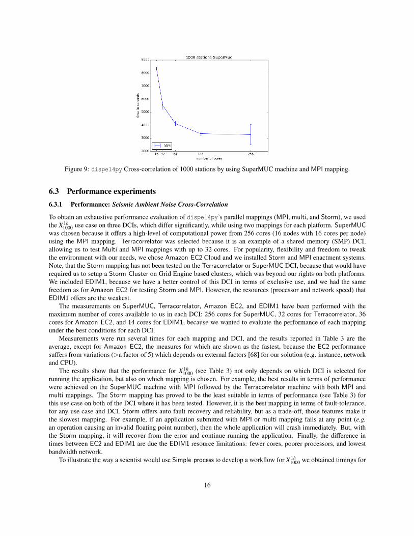
Figure 9: dispel4py Cross-correlation of 1000 stations by using SuperMUC machine and MPI mapping.

6.3 Performance experiments6.3.1 Performance: Seismic Ambient Noise Cross-Correlation

To obtain an exhaustive performance evaluation of dispel4py’s parallel mappings (MPI, multi, and Storm), we usedthe X1h

1000 use case on three DCIs, which differ significantly, while using two mappings for each platform. SuperMUCwas chosen because it offers a high-level of computational power from 256 cores (16 nodes with 16 cores per node)using the MPI mapping. Terracorrelator was selected because it is an example of a shared memory (SMP) DCI,allowing us to test Multi and MPI mappings with up to 32 cores. For popularity, flexibility and freedom to tweakthe environment with our needs, we chose Amazon EC2 Cloud and we installed Storm and MPI enactment systems.Note, that the Storm mapping has not been tested on the Terracorrelator or SuperMUC DCI, because that would haverequired us to setup a Storm Cluster on Grid Engine based clusters, which was beyond our rights on both platforms.We included EDIM1, because we have a better control of this DCI in terms of exclusive use, and we had the samefreedom as for Amazon EC2 for testing Storm and MPI. However, the resources (processor and network speed) thatEDIM1 offers are the weakest.

The measurements on SuperMUC, Terracorrelator, Amazon EC2, and EDIM1 have been performed with themaximum number of cores available to us in each DCI: 256 cores for SuperMUC, 32 cores for Terracorrelator, 36cores for Amazon EC2, and 14 cores for EDIM1, because we wanted to evaluate the performance of each mappingunder the best conditions for each DCI.

Measurements were run several times for each mapping and DCI, and the results reported in Table 3 are theaverage, except for Amazon EC2, the measures for which are shown as the fastest, because the EC2 performancesuffers from variations (>a factor of 5) which depends on external factors [68] for our solution (e.g. instance, networkand CPU).

The results show that the performance for X1h1000 (see Table 3) not only depends on which DCI is selected for

running the application, but also on which mapping is chosen. For example, the best results in terms of performancewere achieved on the SuperMUC machine with MPI followed by the Terracorrelator machine with both MPI andmulti mappings. The Storm mapping has proved to be the least suitable in terms of performance (see Table 3) forthis use case on both of the DCI where it has been tested. However, it is the best mapping in terms of fault-tolerance,for any use case and DCI. Storm offers auto fault recovery and reliability, but as a trade-off, those features make itthe slowest mapping. For example, if an application submitted with MPI or multi mapping fails at any point (e.g.an operation causing an invalid floating point number), then the whole application will crash immediately. But, withthe Storm mapping, it will recover from the error and continue running the application. Finally, the difference intimes between EC2 and EDIM1 are due the EDIM1 resource limitations: fewer cores, poorer processors, and lowestbandwidth network.

To illustrate the way a scientist would use Simple process to develop a workflow for X1h1000 we obtained timings for

16

Measurement platformMode Terracorrelator Amazon

EC2EDIM1 SuperMUC

MPI 3,066 16,863 38,657 1,093multi 3,144Storm 27,899 120,077

Table 3: Elapsed time (in seconds) for X1h1000 on four DCI using the maximum number of cores available

X1h5 ; these are 88 seconds by a Mac OS X 10.9.5 laptop, with processor 1.7GHz Intel Core i5 and 8GB RAM using

release 2.7 of the Python system32.

6.3.2 Performance: Internal Extinction of Galaxies

Initially, we compared the time-to-complete for both implementations (Taverna vs dispel4py), performing a set ofexecutions using the same desktop machine, with 4 GB RAM, an Intel Core 2 Duo 2.66GHz processor, and ensuringthe same network conditions, checking that the VO service is running, and executing them in the same time slot. Thenumber of jobs executed concurrently was set to 10 in the Taverna workflow, since after several tests, we verified thiswas its optimal configuration. dispel4py was configured to use the multi mapping and 4 processes. The differencein elapsed time is considerable. While the Taverna execution takes approximately 9.5 minutes, dispel4py takes 1.7minutes.

Measurement platformMode Terracorrelator EDIM1

MPI 32 96multi 14 101Storm 30

Table 4: Elapsed times (seconds) for 1,050 galaxies on two DCIs with the maximum number of cores available

Further evaluations were performed using the Terracorrelator and EDIM1 DCIs, and the results show (see Table 4) thatthe lowest elapsed time for this workflow was achieved using the multi mapping on the Terracorrelator, followed byStorm on EDIM1. For those evaluations we used the maximum number of cores available in each DCI (see Table 1).The performance differences for the MPI and multi mappings between Terracorrelator and EDIM are due to thenumber and features of the cores available in each DCI. We used 14 cores for the MPI mapping and 4 cores for themulti mapping on EDIM1, and 32 cores for both mappings on the Terracorrelator.

6.3.3 Performance: Twitter Sentiment Analysis

The results shown in Table 5 demonstrate that dispel4py is able to map to diverse DCIs and enactment systems,adapting automatically to their variations, and show that the performance depends on the DCI selected and that thesame use case can run faster or slower depending on the selection of DCI and dispel4py mapping made.

Measurement platformMode Terracorrelator EDIM1 SuperMUC

MPI 925 32,396 2,058multi 971 3,955

Table 5: Elapsed times (seconds) for 126,826 tweets on three DCIs with the maximum number of cores available

32When comparing this with times in Table 3 note that correlation is of O(n2), where n is the number of sources (subscript in the notation X1h5 ).

17

6.4 Analysis of measurementsThe major features of the measured results are summarized in Table 6.

Measurement platformLoad Mode Terracorrelator SuperMUC Amazon EC2 OSDC sullivan EDIM1

simple 1,420X180d

2 MPI 242 173 613multi 218 203 325MPI 3,066 1,093 16,863 38,657

X1h1000 multi 3,144

Storm 27,898 120,077MPI 32 96

int ext multi 14 101Storm 30MPI 952 2,058 32,396

twitter multi 971 3,955

Table 6: Highlights as best average elapsed times for various loads on multiple DCIs

Machine X90d2 X180d

2Terracorrelator 0.44 0.52

SuperMUC 0.67 0.64OSDC 0.43 0.84

Table 7: Parallelization efficiency values for MPI mapping for two sample loads on three DCI.

To assess dispel4py’s automatic parallelisation, we calculated the efficiency of the MPI mapping by using thexcorr workflow and and assessed its parallelisation efficiency using Equation (1) below, as this is an established methodin HPC for measuring scalability of an application. As shown in Table 7, for large datasets the efficiency is at over40% on all platforms.

Time 4processesTime 32processes∗ 32

4

(1)

The results overall show that: a) the same dispel4py workflow can be used unchanged with different map-pings, b) the scalability achieved demonstrates the power of data streaming for data-intensive workloads, c) that thedispel4py Python library provides access to this power for scientists, both when they are developing and when theyare running in production mode their automated scientific methods, and d) mapping to different target DCIs is essentialto handle the variety of workloads—exploiting effectively the features of the target DCIs.

The strategy of depending solely on the Python environment during development and early tests pays off becauseusers can install this on their computer very easily and without the need for technical help. This effectively lowersthe intellectual barrier to getting started, particularly for those already adept and using Python. Though the Pythoninformation is well crafted and the Python community very helpful if a would be dispel4py user is not familiarwith Python. The automated mapping to other target computing infrastructures smooths the path to more demandingevaluations and eventual production deployment. Hence the application of innovations developed in dispel4py isaccelerated and can be achieved by practitioners who don’t have local experts to solve system issues and to optimizetheir methods for particular target computing infrastructures. In most cases those target infrastructures will be onshared clusters. Consequently, the data-intensive frameworks and libraries will have to be set up by the system’sadministrators to comply with security policies.

The present repertoire of supported mappings (with Apache Spark being prototyped) satisfies a large number ofapplications. The current mappings are remarkably efficient even though they do not analyze past performance toestimate costs more accurately. Such an upgrade to the mappings is also being prototyped. The strategy of avoiding

18

(disk) IO clearly pays off in contexts where fast inter-process communication is well supported (in memory or fastinterconnect). That gain is lost when, in contexts such as Storm, data is being preserved for recovery. Coupling suchdata preservation for recovery into the abstract graph could reduce this effect by being selective and strategic in thechoice of locations for recovery – trading potential work lost against recovery overhead. Today, it is possible for theauthor of a dispel4py workflow to do this, but it requires care and effort. A PE library and a tool that supportedsuch recovery strategies would be worthwhile, and the graphs produced could thn be mapped to the highly developedframeworks for data-intensive work, such as Storm and Spark. This would get the best of both worlds.

7 Conclusions and future workSection 1 identified three demanding requirements that should be met by dispel4py, a novel Python library forautomating data-intensive research methods. We have demonstrated that all three requirements are met. The usersof dispel4py have been able to express their computations and data handling as fine-grained abstract workflows.They have been able to use development environments, and tools such as iPython to create and refine sophisticateddata-intensive methods. They have been able to complete this work themselves or integrate developments producedby other experts via the standard Python library mechanisms. The automatic mapping of their workflows withoutmodification to a wide range of computing and data infrastructures empowers researchers with smooth transitionsbetween development and production. This is achieved because the workflow source definition is unchanged. As aconsequence transitions from the lightweight development context are not delayed waiting for expert help to insertoptimizations and details specific to the target, the user just submits the workflow to a different target. Similarly, if auser retrieves a copy of a production workflow to refine a method or develop a related method, that user is not confusedby those inserted details and does not need to reverse the changes.

We argue that data-streaming has long-term value in lightweight coupling of the stages of research methods, inhandling live data streams, and in achieving high-performance data-intensive processing. Three realistic scenarioswere illustrated from the fields of seismology, astrophysics and social computation. These were used to measure theperformance and scalability achieved when dispel4py workflows are mapped to the MPI, Multiprocessing, Stormand Sequential modes running on five different distributed computing infrastructures. It is clear that the underly-ing differences in technology are exploited effectively and that impressive speedups and delivered performance isachieved. Table 6 illustrates this well, showing the best performance achieved on each target platform with differentdata-intensive frameworks. Significant differences appear. Some are explained by the properties of the underlyinghardware. But the TerraCorrelator, designed for data-intensive work with moderate cost and energy consumptioncompared with SuperMUC, shows consistently reasonable elapsed times, outperforming SuperMUC in some cases.The target data-intensive framework also has a significant effect, with Storm significantly slower than MPI on the twoinfrastructures on which we measured them both. User communities will often choose a platform because of theirapplication domain’s shared provision, or because they have entitlement on their project’s or institution’s resources.The efficient accommodation of multiple target mappings means that their needs and constraints can usually be metquite easily.

The next stages of the dispel4py open-source project’s development will include: a) providing a registry systemto assist in the description and sharing of PEs and re-usable workflow fragments, b) developing additional diagnostictools, including graph visualisation and user-controlled monitoring, c) expanding the existing system of provenancecollecting and provenance-driven tools, d) developing a planner that can select the best target DCIs and enactmentmodes automatically, building on systematically garnered and analysed data about previous enactments, and e) ex-tending the community of developers and users to improve dispel4py’s future sustainability. We seek to deploy andevaluate dispel4py in a wide range of scientific and commercial domains. It is an open source project and we wouldwelcome collaborators in steering its development. Our aim will remain delivering products, tools and technologies,to practitioners in many application disciplines to empower them to develop and conduct their own data-intensiveresearch. We will be happy to help but we should not be needed.

19

AcknowledgmentsThis research was supported by the VERCE project (EU FP7 RI 283543), the TerraCorrelator project (funded byNERC NE/L012979/1), with major contributions from the Open Cloud Consortium (OCC) funded by by grants fromGordon and Betty Moore Foundation and the National Science Foundation, and led by the University of Chicago.

References[1] A. J. G. Hey, S. Tansley, and K. Tolle, The Fourth Paradigm: Data-Intensive Scientific Discovery. Microsoft Research, 2009.

[2] T. Segaran and J. Hammerbacher, Beautiful Data: The Stories Behind Elegant Data Solutions. O’Reilly, 2009.

[3] A. Shoshani and D. Rotem, Scientific Data Management: Challenges, Technology and Deployment. Chapman & Hall, 2010.

[4] W. H. Dutton and P. W. Jeffreys, World Wide Research: Reshaping the Sciences and Humanities. MIT Press, 2010.

[5] M. Atkinson and M. Parsons, “The digital-data challenge,” in [6]. Wiley, 2013, ch. 1, pp. 5–13.

[6] M. P. Atkinson et al., The DATA Bonanza – Improving Knowledge Discovery for Science, Engineering and Business. Wiley, 2013.

[7] H. Koepke, “Why Python rocks for research,” University of Washington, Tech. Rep., 2014.

[8] A. Ringler et al., “The data quality analyzer: A quality control program for seismic data,” Computers & Geosciences, vol. 76, pp. 96–111, 2015.

[9] P. S. Earle et al., “Prompt Assessment of Global Earthquakes for Response (PAGER): A system for rapidly determining the impact of earthquakes worldwide,” USGeological Survey, Tech. Rep., 2009.

[10] C. Walter, “Kryder’s Law,” Scientific American, pp. 32–33, August 2005.

[11] R. Filgueira et al., “Applying selectively parallel io compression to parallel storage systems,” in Euro-Par, 2014.

[12] A. Barker et al., “Choreographing web services,” IEEE Trans. on Services Computing, vol. 2, no. 2, pp. 152–166, 2009.

[13] MPI Forum, “MPI: A message-passing interface standard,” IJ of Supercomputer Applications, vol. 8, pp. 165–414, 1994.

[14] E. Deelman et al., “Pegasus, a workflow management system for science automation,” Future Generation Computer Systems, no. 0, pp. –, 2014.

[15] B. Ludascher et al., “Scientific workflow management and the Kepler system,” Concurrency and Computation: P&E, vol. 18, no. 10, pp. 1039–1065, 2006.

[16] M. Wilde et al., “Swift: A language for distributed parallel scripting,” Parallel Comp., vol. 37, no. 9, pp. 633 – 652, 2011.

[17] S. Beisken et al., “KNIME-CDK: Workflow-driven cheminformatics,” BMC Bioinformatics, vol. 14, no. 1, p. 257, 2013.

[18] M. R. Berthold et al., “KNIME - The Konstanz Information Miner,” SIGKDD Explor., vol. 11, no. 1, pp. 26–31, 2009.

[19] K. Wolstencroft et al., “The Taverna workflow suite: designing and executing workflows of Web Services on the desktop, web or in the cloud,” Nucleic AcidsResearch, vol. 41, no. W1, pp. W557–W561, 2013.

[20] D. Blankenberg et al., Galaxy: A Web-Based Genome Analysis Tool for Experimentalists. Wiley, 2010.

[21] Y. Simmhan et al., “Building the Trident Scientific Workflow Workbench for Data Management in the Cloud,” in ADVCOMP. IEEE, October 2009.

[22] D. Churches et al., “Programming scientific and distributed workflow with Triana services,” Conc.&Comp.: P&E, vol. 18, no. 10, pp. 1021–1037, 2006.

[23] M. Kozlovszky et al., “DCI Bridge: Executing WS-PGRADE Workflows in Distributed Computing Infrastructures,” in [25], P. Kacsuk, Ed. Springer, 2014,ch. 4, pp. 51–67.

[24] K. Vahi et al., “Rethinking Data Management for Big Data Scientific Workflows,” in Workshop on Big Data and Science: Infrastructure and Services, 2013.

[25] P. Kacsuk, Ed., Science Gateways for Distributed Computing Infrastructures: Development framework and exploitation by scientific user communities. Springer,2014.

[26] G. B. Berriman et al., “The application of cloud computing to the creation of image mosaics and management of their provenance,” in Software and Cyberinfras-tructure for Astronomy, vol. 7740. SPIE, 2010, p. 77401F.

[27] M. Rynge et al., “Producing an Infrared Multiwavelength Galactic Plane Atlas using Montage, Pegasus and Amazon Web Services,” in ADASS Conf., 2013.

[28] G. B. Berriman et al., “Generating Complex Astronomy Woret al.,kflows,” in Workflows for e-Science. Springer.

[29] D. Gannon et al., “Dynamic, Adaptive Workflows for Mesoscale Meteorology,” in [30]. Springer, 2007, pp. 126–142.

[30] I. J. Taylor et al., Workflows for e-Science: Scientific Workflows for Grids. Springer, 2007.

[31] S. Aiche et al., “Workflows for automated downstream data analysis and visualization in large-scale computational mass spectrometry,” Proteomics, 2015.

[32] P. Maechling et al., “SCEC CyberShake Workflows—Automating Probabilistic Seismic Hazard Analysis Calculations,” in [30]. Springer, 2007, pp. 143–163.

[33] D. Barseghian et al., “Workflows and extensions to the Kepler scientific workflow system to support environmental sensor data access and analysis,” EcologicalInformatics, vol. 5, pp. 42–50, 2010.

20

[34] S. Kelling et al., “Estimating species distributions – across space, through time and with features of the environment,” in [6]. Wiley, 2013, ch. 22, pp. 441–458.

[35] C. Buil-Aranda et al., “Federating Queries in SPARQL1.1:Syntax, Semantics and Evaluation,” Web Semantics, vol. 18, no. 0, 2013.

[36] M. Stonebraker et al., “SciDB: A DBMS for Applications with Complex Analytics,” Comp. in Sci.&Eng., vol. 15, no. 3, pp. 54–62, 2013.

[37] D. De Roure and C. Goble, “Software design for empowering scientists,” IEEE Software, vol. 26, no. 1, pp. 88–95, 2009.

[38] S. Kohler et al., “Sliding Window Calculations on Streaming Data using the Kepler Scientific Workflow System,” Procedia Computer Science, vol. 9, no. 0, pp.1639 – 1646, 2012.

[39] B. Acs et al., “A general approach to data-intensive computing using the Meandre component-based framework,” in Proc. 1st Int. Workshop on Workflow Ap-proaches to New Data-centric Science. ACM, 2010, pp. 8:1–8:12.

[40] M. P. Atkinson, “Data-Intensive thinking with Dispel,” in [6]. Wiley, 2013, ch. 4, pp. 61–122.

[41] M. P. Atkinson et al., “Data-intensive architecture for scientific knowledge discovery,” Distributed and Parallel Databases, vol. 30, no. 5-6, pp. 307–324, 2012.

[42] Z. Falt et al., “Bobolang: A Language for Parallel Streaming Applications,” in Proc. HPDC. ACM, 2014, pp. 311–314.

[43] M. Carpene et al., “Towards Addressing CPU-Intensive Seismological Applications in Europe,” in Supercomputing. Springer, 2013, vol. 7905, pp. 55–66.

[44] B. Agarwalla et al., “Streamline: scheduling streaming applications in a wide area environment,” in Multimedia Systems, vol. 13, 2007, pp. 69–85.

[45] K. Agrawal et al., “Mapping filtering streaming applications,” Algorithmica, vol. 62, no. 1-2, pp. 258–308, 2012.

[46] F. Guirado et al., “Enhancing throughput for streaming applications running on cluster systems,” J. Par. Distrib. Comp., vol. 73, no. 8, pp. 1092–1105, 2013.

[47] S. G. Ahmad et al., “Data-Intensive Workflow Optimization based on Application Task Graph Partitioning in Heterogeneous Computing Systems,” in 4th IEEEInt.l conf. on Big Data and Cloud Computing, 2014.

[48] J. M. Wozniak et al., “Turbine: A distributed-memory dataflow engine for high performance many-task applications,” Fundamenta Informaticae, vol. 128, no. 3,pp. 337–366, 01 2013.

[49] D. De Roure et al., “The Design and Realisation of the myExperiment Virtual Research Environment for Social Sharing of Workflows,” FGCS, vol. 25, pp.561–567, 2009.

[50] K. Belhajjame et al., “A Suite of Ontologies for Preserving Workflow-Centric Research Objects,” J. Web Semantics, in press 2015.

[51] D. Garijo et al., “Workflow reuse in practice: A study of neuroimaging pipeline users,” in 10th IEEE International Conference on e-Science, eScience 2014, SaoPaulo, Brazil, October 20-24, 2014, 2014, pp. 239–246. [Online]. Available: http://dx.doi.org/10.1109/eScience.2014.33

[52] L. Lefort et al., “W3C Incubator Group Report – review of Sensor and Observation ontologies,” W3C, Tech. Rep., 2010.

[53] D. Rogers et al., “Bundle and Pool Architecture for Multi-Language, Robust, Scalable Workflow Executions,” J. Grid Comput., vol. 11, no. 3, pp. 457–480, 2013.

[54] A. Spinuso et al., “Provenance for seismological processing pipelines in a distributed streaming workflow,” in Proc. EDBT ’13. ACM, 2013, pp. 307–312.

[55] S. Gesing et al., “Workflows in a Dashboard: A New Generation of Usability,” in Proc. WORKS’14. IEEE, 2014, pp. 82–93.

[56] R. Filgueira et al., “dispel4py: An agile framework for data-intensive escience,” in Proc. IEEE eScience 2015, 2015.

[57] M. P. Atkinson et al., “VERCE delivers a productive e-Science environment for seismology research,” in Proc. 11th IEEE eScience Conf., 2015.

[58] G. D. Bensen et al., “Processing seismic ambient noise data to obtain reliable broad-band surface wave dispersion measurements,” Geophysical Journal Interna-tional, vol. 169, no. 3, pp. 1239–1260, 2007.

[59] “SEED Reference Manual v2.4, Appendix G: Data Only SEED Volumes (Mini-SEED),” http://www.iris.edu/ manuals/ SEED appG.htm, accessed August 2011.

[60] M. Beyreuther et al., “ObsPy: A Python Toolbox for Seismology,” Seismological Research Letters, vol. 81, no. 3, pp. 530–533, 2010.

[61] M. Bode et al., The ASTRONET Infrastructure Roadmap. ASTRONET, 2008. [Online]. Available: http://books.google.co.uk/books?id=Y5tQPgAACAAJ

[62] J. Ruiz et al., “Astrotaverna - building workflows with virtual observatory services,” Astronomy and Computing, vol. 7–8, no. 0, pp. 3–11, 2014, special Issue onThe Virtual Observatory: I.

[63] A. Pak and P. Paroubek, “Twitter as a corpus for sentiment analysis and opinion mining,” in Proceedings of the International Conference on Language Resourcesand Evaluation, LREC 2010, 17-23 May 2010, Valletta, Malta, N. Calzolari, K. Choukri, B. Maegaard, J. Mariani, J. Odijk, S. Piperidis, M. Rosner, andD. Tapias, Eds. European Language Resources Association, 2010. [Online]. Available: http://www.lrec-conf.org/proceedings/lrec2010/summaries/385.html

[64] W. Medhat, A. Hassan, and H. Korashy, “Sentiment analysis algorithms and applications: A survey,” Ain Shams Engineering Journal, vol. 5, no. 4, pp. 1093 –1113, 2014. [Online]. Available: http://www.sciencedirect.com/science/article/pii/S2090447914000550

[65] H. Cho, J. Lee, and S. Kim, “Enhancing lexicon-based review classification by merging and revising sentiment dictionaries,” in Sixth International JointConference on Natural Language Processing, IJCNLP 2013, Nagoya, Japan, October 14-18, 2013. Asian Federation of Natural Language Processing / ACL,2013, pp. 463–470. [Online]. Available: http://aclweb.org/anthology/I/I13/I13-1053.pdf

[66] F. A. Nielsen, “Afinn,” Richard Petersens Plads, Building 321, DK-2800 Kgs. Lyngby, mar 2011.

[67] S. Baccianella, A. Esuli, and F. Sebastiani, “Sentiwordnet 3.0: An enhanced lexical resource for sentiment analysis and opinion mining,” in Proceedings of theSeventh International Conference on Language Resources and Evaluation (LREC’10), May 2010.

[68] A. Le-Quoc et al., “The top 5 aws ec2 performance problems,” http://www.datadoghq.com/wp-content/uploads/2013/07/top 5 aws ec2 performance problems ebook.pdf,2013.

21