edgeworth expansions for sampling without replacement from

JOURNAL OF MULTIVARIATE ANALYSIS 17, 261-278 (1985)

Edgeworth Expansions for Sampling without Replacement from Finite Populations

G. JOGESH BABU* AND KESAR SINGH+

Rutgers University

Communicated by J. Pfanzagl

The validity of the one-term Edgeworth expansion is proved for the multivariate mean of a random sample drawn without replacement under a limiting non-latticeness condition on the population. The theorem is applied to deduce the one- term expansion for the univariate statistics which can be expressed in a certain linear plus quadratic form. An application of the results to the theory of bootstrap is mentioned. A one-term expansion is also proved in the univariate lattice case. 0 1985 Academic Press, Inc.

1. INTRODUCTION AND MAIN RESULTS

Let { Ui, UZ,..., U,} be a finite population, i.e., a finite collection of N distinguishable objects. Let u,, uZ,..., u, denote a random sample of size n drawn without replacement from this population. Let X be a (row) vector of k variables; Xi = (Xi, ,..., X,) is the value of Xfor Ui. Let xi denote the X measurement on the sampled unit ui. In this study, we consider the problem of Edgeworth expansions for a class of statistics based on the data (x,, x2,..., x,). The main finding of this paper is the validity of the one-term Edgeworth expansion under an intuitive condition of limiting non-latticeness. Here the limit is taken as the sample size n (which may depend upon N) tends to co in such a fashion that (n/N) 6 1 - 6, for a 6 > 0. The Erdos-RCnyi formula for the characteristic function of a sample sum in the above situation is one of the key tools in this study.

Before getting to the specific findings of this paper let us have a brief look at the related literature. Erdijs and RCnyi [8] proved probably the

Received November 8, 1982; revised March 30, 1984. AMS 1970 subject classifications: 62E20, 62DOS. Key words and phrases: edgeworth expansions, sampling without replacement, weak con-

vergence, characteristic functions, ratio estimators, lattice distributions, rank tests. * On leave from the Indian Statistical Institute. + Research supported by NSF Grants MCS-81-02341 and MCS-8301082.

261 0047-259X/85 S3.00

Copyright 0 1985 by Academic Press. Inc. All rights of reproduction in any form reserved.

262 BABU AND SINGH

first satisfactory CLT for sampling without replacement. This paper came up with an ingenious formula for the c.f.‘s of the sum of a random sample drawn without replacement. The formula has been used in a number of related studies. Few references of earlier results on the CLT are cited in the above article. See Hajek [ 12, 131 and Rosen [16, 171 for further works on the first-order limit theory for rejective sampling schemes. Robinson [15] has a theorem on Edgeworth expansion in the case of one-dimensional mean. We may comment here that the Condition (C) of Robinson’s paper, though verifiable when one is dealing with the two sample rank tests, appears too technical to visualize in the case of a natural population. Bickel and van Zwet [6] also contains some results on Edgeworth expansion for sampling without replacement under conditions similar to that of Robinson. The expansions in the latter paper were obtained in the context of higher-order asymptotics for two sample rank tests.

The following are some of the notations used in this text. For a vector p = (p, ,..., fik) of non-negative integers, let I/?1 = /I, + . . . + Pk, p! = pl ! fi2 !... fik !, DB = Dfl 04 *+. Dp where Dp before a function stands for the Pith partial derivative with respect to the ith variable, xB = xfIx$ . . xp for x = (x1 ,..., xk). The usual Euclidean norm is denoted by 11 11, and the inner product of two vectors c1 and fl is denoted by a. /I. @= and 4x denote the d.f. and the density of the normal distribution with mean 0 and dispersion C; 0 and 4 are the d.f. and the density function of the standard normal distribution on the real line. Let F, be the d.f. on [Wk which assigns mass l/N to each of the points X,, X, ,..., X,. Let p = n/N and q = 1 - p. For a function f on [Wk, ENf is the mean of f under FN; Z:, = E,(X- E,X)‘(X- E,X). Let

and df, E, Y)=suP{lf(.Y-fW Ilv-4 G&l

$f, 6 C) = s df, 6 Y) d@,(Y) for a real-valued measurable function f on lRk. The d.f. of Z,, where Z, = (nq)-“* C; (xi- E,X), is denoted by Q,. The one-term Edgeworth expansion for Q,, is the signed measure P, whose density is

dzx(~) - (9 -P)(nq)F”2pN(y)p

PN (Y) = c +, EdX- &4BDB4,,(~)- IPI= .

Now, we state the one-term expansion for Qn as

THEOREM 1. If ENllXll 3 +’ is bounded and (n/N) < 1 - 6 for some 6 > 0 as N -+ 00 and FN converges weakly to a s.n.1. (strongly non-lattice) dis-

EDGEWORTH EXPANSIONS 263

tribution F on IWk, then, for any bounded measurable function f, there exists a sequence 6, = o(n-‘I’) s.1.

where 6,, the constant c and the o(n112) term depend on f only through its upper bound.

Although our primary interest in this article lies in the expansion of Q,(A) for certain Bore1 measurable subsets of IWk, Theorem 1 is required in the present integral form in order to deduce the next theorem from it.

The condition of s.n.1. weak limit can be relaxed slightly. The proof of Theorem 1 goes through if one assumes that there exists a measurable sub- set A of [Wk s.t. lim inf F,(A) > 0 and the conditional distribution of F, on A has a s.n.1. weak limit. Roughly speaking, the latter condition amounts in practice to assuming that the central portion of the population is more or less smooth.

It is not clear at this point if it is possible to obtain more than one-term expansion for Q,, under the condition of a weak convergence of FN. However, if one assumes that {X,, X2,..., X,} is a random sample from a population which satisfies Cramer’s condition, then the proofs of this article can easily be modied to obtain a k-term expansion. Incidently, the assumption that {Xi, X2,..., X,} is a random sample from an appropriate population is known as a superpopulation model in the sample-survey literature. A considerable number of studies have been carried out under superpopulation models.

A fairly large class of statistics used in sample surveys including serveral studentized functions of the multivariate sample means, can be expressed as I.Z, +n-“‘Z,LZh + op(n-‘/2) where I is a 1 x k vector and L is a k x k matrix. We apply Theorem 1 to deduce the one-term expansion for this class of statistics. The result is formally stated as

THEOREM 2. Let the conditions of Theorem 1 hold. Assume that a univariate statistic T,, can be decomposed as T,, + R, where T,, = 1. Z, + n-‘12Z, LZL and R, is such that P( 1 R,I 2 a,) = o(n- ‘I*) for a positive sequence (a,} which itself is o(n-‘I*). Let o’, be IC,l’. Ifmax(Il,I, L,L IQ’I) ’ b ts oun e d d as n, N -+ 00, where l= (1, ,..., lk) and ((L,)) = L, then

~(T,~o,Y)=@(Y)-~(Y) &Y)+oW"~)

where ?j( y) = ON ‘E( F,,) + ( l/64,)( y2 - 1) E( r, - J!%‘,)~. In fact

E,T,,=n-“2tr(C,L)+o(n~“2) (tr stands for the trace of a matrix) (1)

264 BABUANDSINGH

and

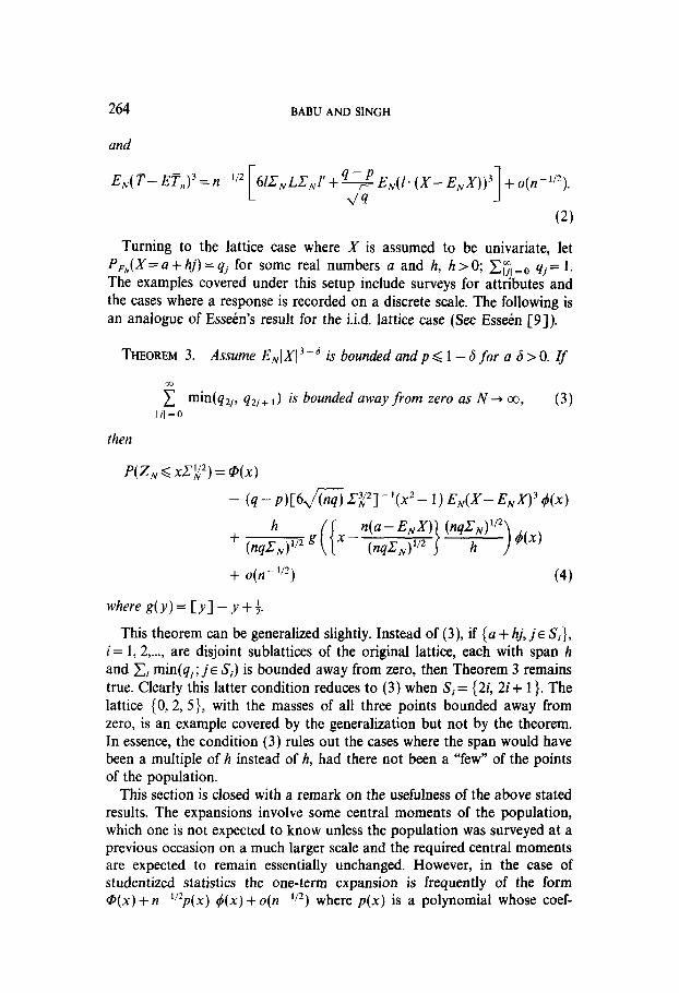
E,(T-ET”)3=n-1’2 6l,Z,LC,,,P+4-p EN(I.(X-E X))3 [ A

N 1

+o(n-‘I’).

(2)

Turning to the lattice case where X is assumed to be univariate, let P,(X = a + hj) = qj for some real numbers a and h, h > 0; C; = 0 qj = 1. The examples covered under this setup include surveys for attributes and the cases where a response is recorded on a discrete scale. The following is an analogue of Esseen’s result for the i.i.d. lattice case (See Essdn [9]).

THEOREM 3. Assume ENIX13+’ is bounded andp< l-6 for a 6>0. If

C min(q2j, qZj+l ) is bounded away from zero as N + a~, IA =O

(3)

then

P(z, 6 &,!‘) = @(x) - (4 - P~~~~~~*I -‘(x2 - 1) E,wV-- &-J’)3 4(x)

h

+ (nqzN)“* g

+ o(n - 1’2)

whereg(y)=[y]-y+f

(4)

This theorem can be generalized slightly. Instead of (3), if (a + hj, je S,}, i = 1, 2,..., are disjoint sublattices of the original lattice, each with span h and xi min(qj; Jo Si) is bounded away from zero, then Theorem 3 remains true. Clearly this latter condition reduces to (3) when Si = (2i, 2i + 1 }. The lattice {0,2, 5}, with the masses of all three points bounded away from zero, is an example covered by the generalization but not by the theorem. In essence, the condition (3) rules out the cases where the span would have been a multiple of h instead of h, had there not been a “few” of the points of the population.

This section is closed with a remark on the usefulness of the above stated results. The expansions involve some central moments of the population, which one is not expected to know unless the population was surveyed at a previous occasion on a much larger scale and the required central moments are expected to remain essentially unchanged. However, in the case of studentized statistics the one-term expansion is frequently of the form a(x) + n-“*p(x) b(x) + o(n-‘I*) where p(x) is a polynomial whose coef-


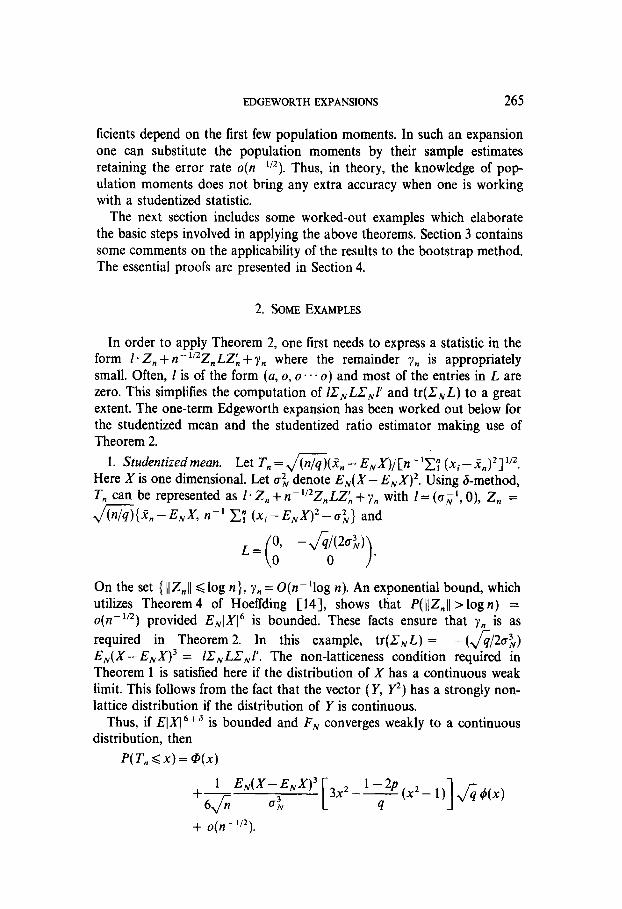
ficients depend on the first few population moments. In such an expansion one can substitute the population moments by their sample estimates retaining the error rate o(c”~). Thus, in theory, the knowledge of population moments does not bring any extra accuracy when one is working with a studentized statistic.

The next section includes some worked-out examples which elaborate the basic steps involved in applying the above theorems. Section 3 contains some comments on the applicability of the results to the bootstrap method. The essential proofs are presented in Section 4.

2. SOME EXAMPLES

In order to apply Theorem 2, one first needs to express a statistic in the form 1.2, + ~I-‘/~Z,,LZ:, + Y,, where the remainder yn is appropriately small. Often, I is of the form (a, o, 0.. . o) and most of the entries in L are zero. This simplifies the computation of lC,.,LEJ and tr(C,L) to a great extent. The one-term Edgeworth expansion has been worked out below for the studentized mean and the studentized ratio estimator making use of Theorem 2.

1. Studentized mean. Let T, = J7n/4)(2, - E,X)/[n-‘ET (x~-.~J~]*‘~. Here X is one dimensional. Let 0; denote E,,,(X- E,X)2. Using d-method, T, can be represented as 1.2, + K’/~Z,LZ:, -I- yn with 1= (a,‘, O), Z, =

,/6?8{%-Ed, n-l C; (Xi - ENX)2 - CL} and

L = ( 0, -&d) 0 ) 0 .

On the set { IIZ,,I( <log n>, y, = O(n-‘log n). An exponential bound, which utilizes Theorem 4 of Hoeffding [ 141, shows that P( JIZ,,II > log n) = o(n-‘12) provided E,(X16 is bounded. These facts ensure that y,, is as required in Theorem 2. In this example, tr(X,L) = -(h/20;) E,(X- E,X)3 = LZ’, LCJ’. The non-latticeness condition required in Theorem 1 is satisfied here if the distribution of X has a continuous weak limit. This follows from the fact that the vector (Y, Y2) has a strongly non- lattice distribution if the distribution of Y is continuous.

Thus, if EIX16+’ is bounded and F,,, converges weakly to a continuous distribution, then

P( T, <x) = G(x)

266 BABU AND SINGH

2. Studentized ratio estimator. Let Y be the variable under study and X be an auxiliary variable. Let X and Y both be one dimensional. Consider

T,=JGGC(~/-~)ENX-ENYI

I[

n-l iCYi--(J/-f)Xi)* .

I

112

1

Let R = E, Y/E,X. Let DC denote EN( Y - RX)* in this example. Here, T,, has the desired representation with 1= (a; ‘, o, o),

Z.=~jn-‘i:(yj-Rxi),n~‘~(gi-Rni)’ 1 I

- o$,n -lfXi-ENXJ 1 J

and

where a=(,,/&),E,X)[E,,,(XY) - RENX2], b = -h/20; and c= -,,&(r,E,,,X). Thus, tr(.Z,L) = lC,LZ,l’ = (&c$E,X)[E,XY - RE,X*] - (4324) E,,,(Y - RX)3 - (J;;Ia,E,X) E,(Y - RX)(X - E,X). Here, the boundedness of E,IX(6+6 and E,IY16+6 is needed in order to apply Theorem 2. The vector [ ( Y - RX), ( Y - RX)*, (X- ENX)] has a strongly non-lattice weak limit if the following holds:

The joint population of (Y, X) has a weak limit which has a non-zero absolutely continuous component.

The one-term expansion in this example can be written explicitly as follows:

,/r, P( T,, < x) = Q(x) + - 60&/G

(x2 - 1) +$ E,,,( Y - RX)3

2

- x2 *E,(XY-RX*)-;E,(Y-Rx)” EN(x)

- & E,(Y- RX)(X- E,X) b(x) + o(n-‘I*). N I>

It may be noted here that quite frequently there are surveys where the auxiliary variable is discrete and the variable under study is continuous. It turns out that in this situation too, the above expansion for the studentized ratio estimators remains valid. To be precise, we need to assume the follow-

EDGEWORTHEXPANSIONS 267

ing for this validity: The auxiliary variable X is concentrated on the points a+hj;j=O, fl,.... The joint distribution of (X, Y) has a weak limit whose marginal corresponding to Y is continuous and that corresponding to X is lattice (with span h). The proof of this claim involves some major modifications in the proof of Theorem 1, which may be presented elsewhere.

3. Studentized sample proportion. Let T, = ,/%&- @l&6% where e^ is the sample proportion of an attribute and 8 is the corresponding population proportion. It is easily checked that

(e^- e) (e^- e) [Qi -Q-p2= ce(i -e)-y-zJ~ &i@2$j

1-a [ 0-e y+op(n-')

where the o&n-‘) term is small enough to be ignored in the one-term expansion. As a result, if Q, is the one-term expansion for P(m (8 - 0)/,/m Qx) then the corresponding expansion for P( T,, < x) is

Q,(x + (q/n)1’2( 1 - 28) x2/2[0(l -0)-J”‘).

It is interesting to note that in the case of attribute sampling one can deduce the one-term expansion for the studentized mean directly from that of the regular mean (8- tI).

3. SOME COMMENTS RELATED TO THE BOOTSTRAP METHOD

The bootstrap procedure in the usual i.i.d. case consists of drawing repeated samples from the expirical population and recomputing the required statistic for the second-stage samples, and replacing the unknown population parameters appearing in the statistic by those of the empirical population. The histogram of a large number of the bootstrap values is used for approximating the true distribution of the statistic. Obviously, if the size of the second-stage samples is to be kept the same as that of the original sample, it would be meaningless to draw random samples without replacement from the usual empirical population. One way to avoid this problem is to sample from an enlarged empirical population 9& made of k copies of {x,, x2 ,..., x,}, for a fixed or a random integer k. The idea of enlarging the empirical population to sample from was first suggested by Gross [ 1 I]. Bickel and Freedman [S], Chao and Lo [7] established various consistency properties of this modified version of bootstrap. In order to match the sampling fraction of the second-stage samples with that of the original sample, the inflating factor k should be chosen as the integer closest to (N/n). In fact, as suggested by the above authors, one may ran-

268 BABU AND SINGH

domize the bootstrap samples between Fntn,rNln, and QN,,,,+ 1 with probabilities p and (1 - p), choosing p such that the finite population correction in the bootstrap variance of the sample mean matches exactly with that in the actual variance.

It was noted in Singh [ 181 and Babu and Singh [ 1,2] that in the i.i.d. setup the bootstrap approximation to the distribution of a studentized statistic is typically equivalent to one-term Edgeworth corrected normal approximation. This phenomenon of one-term Edgeworth correction by the bootstrap is primarily based upon the observation that the conditions assumed on the original population for the validity of the one-term expansion also hold on the empirical population, for all large n (a.s.); and hence one has a valid one-term expansion for the bootstrap distributions. Since a bootstrap statistic is structurally identical to the original statistic, it turns out that the difference of its one-term expansion and that of the original statistic is o(n-‘I*), p rovided the leading terms do not involve any parameter. In the present setup of sampling without replacement, it is well known that the difference of the empirical d.f. and the population d.f. converges to zero. As a result if FN possesses a strongly non-lattice weak limit, then so does the d.f. of 9n,k (which indeed is the same for all k). The only extra item that one needs to take into consideration here is the appearance of sampling fractions in the l/,,& terms. It does not seem likely that the discrepancy caused by the departure of k from (N/n), when the latter is not an integer, can be eliminated in general by any simple randomization of k; though the effect of this discrepancy is not likely to be substantial especially so if the sampling fraction is small to start with. Thus in summary, the one- term correction phenomenon by the bootstrap basically holds in the present setup too.

4. THE PROOFS

We assume without loss of generality that EN(X) =O. In the proofs below c, 6 and E are generic constants; c stands for suIIiciently large positive numbers and E, 6 symbolize appropriately small but positive numbers. We define a sequence a, to be O(*) if a,, = U(n?) for every k > 0; in other words there exists a constant c(k), for every k >O, such that nklanl <c(k).

Proof of Theorem 1. We truncate Xls at &&log n)2. Let X7 denote the truncated and centered Xi’s, i.e.,

xi* = xiz( IlXill < &/(lOg n)‘) - E,Xz( IlXll < &/(lOg 4’).

Let x,? denote the corresponding sample values. If Qz denotes the dis-


tribution of (nq)) ‘I* C; x,+, then for any measurable function f: Rk + [w, bounded by c(f) > 0,

since xi, x2,..., x, are identically distributed and E,,,llXI13+6 = O(1) for a 6 > 0. The difference jj’d(Q,* - P,) is estimated using an inversion result obtained by combining Lemma 11.6 of Bhattacharya and Ranga Rao [4] with Lemma 5 of Sweeting [ 191. The result is formally stated as follows:

LEMMA 1. Let P be a probability on Rk and Q denote a measure with density [ 1 + nl’*pv)] dp( y), w h ere p(y) is a polynomial and Z is a p.d. matrix of order k x k. Let I,,,, 1;; and the coefficients of p( y) be bounded by M > 0, where A,,,,, , Jmin denote the maximum and the minimum eigenvalues of Z. Then for any bounded measurable function f: Rk + R and 6 > 0,

+ c(M) O(f, fW”*, C) + o(n-“*).

Here P and $ stand for the c.f’s of P and Q, and c(k) and c(M) are positive constants. The constants c(k), c(M) and the o(n-‘I*) term depend upon f only through its bound.

The proof of this lemma is deleted. The problem thus reduces to showing that, for any A4 > 0 and IpI <k + 1,

s ,,,,, cM\r l@@,*(t) - ~,Wll dt= oW’*). . n

The above inte ral is estimated in two separate ranges: (I) log n < lltll GM $ n and (II) lltll <log n. In the first range, lDBP,(t)l = O(*). Therefore, in this range, it suffices to show that lD8(j~(t)l is appropriately small. In fact, it is shown in Lemma 3 that this term is O(*) too. The integral over the inner zone is shown to be o(n-“*) through Lemma 4. In Lemma 2, we show that the eigenvalues of Z, and Z$ = ENX*‘X* are bounded below and above if one assumes that F,,, has a s.n.1. weak limit. This latter fact is of critical importance in the proofs of Lemmas 3 and 4.

LEMMA 2. Let 1, and A, denote the smallest and the largest eigenvalues of Z,. As N + co, AN’ and AN are bounded. The same hola3 about 2%.

270 BABUANDSINGH

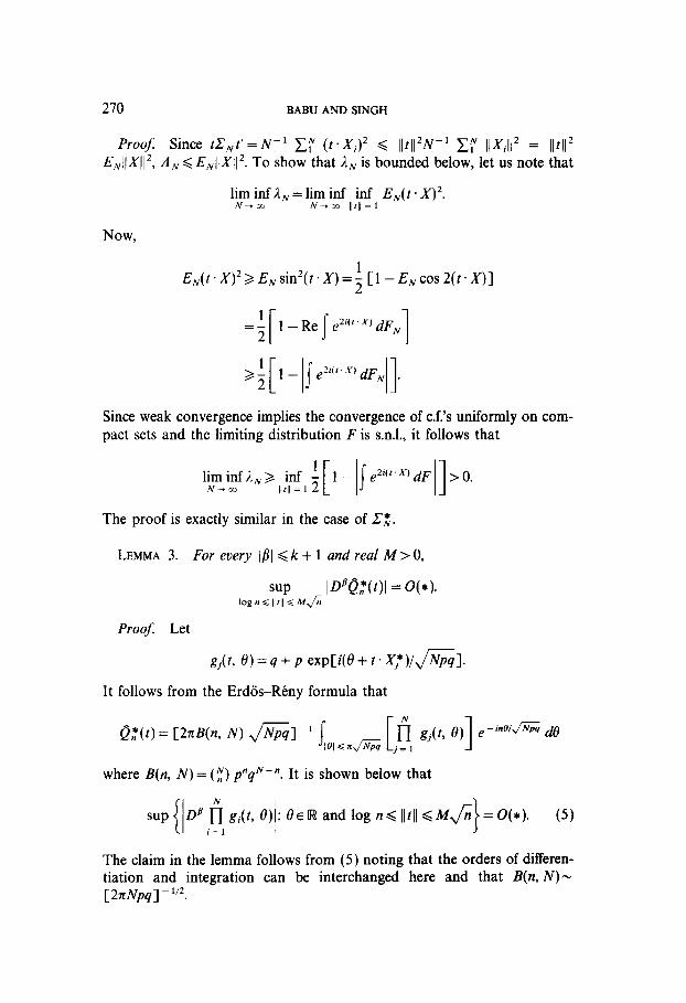
Proof Since tC,t’=N-’ C;” (t.Xi)’ < Iltll’N-’ Cr llXi[l’ = lltl12 E,I(XJI ‘, A,,, < E,IIXI( 2. To show that 1, is bounded below, let us note that

lirn+izf 1, = limizf ,, t:f, EN( t. X)‘. I

Now,

Since weak convergence implies the convergence of c.f.‘s uniformly on com- pact sets and the limiting distribution F is s.n.l., it follows that

l~~~fl,b,,~,nf,~[l-~~~2’(‘X)~F~~>0.

The proof is exactly similar in the case of C,$.

LEMMA 3. For every I/?1 <k + 1 and real M>O,

SUP IDq*(t)l = O(*). n log n < II 111 < MJ;;

Proof: Let

g,(t, O)=q+p exp[i(8+t.X:)/&].

It follows from the Erdos-Riny formula that

where B(n, N) = (z) p”qN-“. It is shown below that

sup DB fi g,(t, 6) : 0~ R and log n< lItI GM& (5) i= 1

The claim in the lemma follows from (5) noting that the orders of differen- tiation and integration can be interchanged here and that B(n, N)- [ 2xNpq] - 1’2.


The derivative DB[n~=, g,(t, e)] (the derivatives are only with respect to t) is a sum of N’B’ terms. Each term is of the form a * b where a is the product of at least (N- 181) of the functions g,(t, 19) and b is the product of certain partial derivatives of the remaining g,(t, 0)‘s. The orders of the partial derivatives add up to l/I1 in each summand. If b is made of the derivatives of j of the functions g,(t, Q, 1 < j < l#Il, then b is bounded by cpj. Note that the number of such terms is at most cN(N- 1). .. (N-j). Thus,

C={l,2 ,... N}-{i,,i, )... i,,,},l<i,< .-.i,,,<N / . (6)

Now, for a C= (1, 2 ,... N} - {i1, i, ,... i,@,},

Gcexp [

-2pqg [i-c0S((e+kx:)lJjVpg)l 1 1

=cexp[-2pqNE,[l-cos((e+t.X*)/JNpg]]. (7)

These estimates are combined with the following lower bounds for E,[l -cos((e+t.X*)/&)] to deduce (5).

lim inf inf ~,[i - c0s((e + t. x*)/Jivpq)-j > 0 N -+ m .9 E W,E Q Iltll/J;; Q M

(8)

and, over 0 < ltl/,f n 6 E for a sufficiently small positive E, there exists a 6 > 0 s.t.

~N[i-cos((e+~‘~*)/JNP(I)]~~litii2/~. (9)

Consider (8) first. The following arguments are similar to the ones employed in Lemma 2.

E~[ i - c0s((e + t. x*)/&)1

al-lENexp[(i6+it.X*)/JX&]l

= 1- IE,exp[it.X*/JNpq]I.

Therefore, in view of the assumed weak convergence of FN,

the left-hand side of (8) 3 inf [l-t?(t)] a, s llfll G “2

(10)

272 BABU AND SINGH

for some positive a1 and u2. Hence, (8) holds. To establish (9), we employ the following estimate based on Taylor’s expansion:

t‘qt’ EN ,ir ‘WJG - 1 + - , 2Npq

<E (t.X*13 “@jp’

This, together with (lo), Lemma 2 and the moment condition E,&Yl13+” = 0( 1 ), implies (9).

LEMMA 4. Over I/ tll 6 log n,

Proof: Using a refined version of Sterling’s formula, it is checked that & B(n, N) = l/,,,% + o(n-“*). Thus,

Q,*(t) = je, gj(t, 0) e-inQ’G de. (11) Because of the following estimatess, the range of integration in (11) can be reduced to Z&/log n, which helps in the later expansions: If 181 B Z&/log n and II t II < log n,

DB fi gi( t, 0) < cnlPl I

1, exp(-pq~[I-eos(e~)])

= O(*)

in view of the definition of X*‘s, (6) and (7). For estimating @[Q,*(t) - P,(t)], the following representation of @P,(t) has been made use of:

&iDBB,(t)-[ DB exp - 4 - t.zy - i$(e, t) de IQ1 i %&aog n > I

= o(n-‘12) exp( --Ellt(12)

where $(t, e)= (q-p)[e3+ 3etzgt’+E,(ta*)3]/6JNpq. In the remainder of the proof we show that

fi g,(t, tJ)e-ineIfi-exp

j= I

Mt, e) )II = o(n -‘12) exp[ -4 llt112 + e2)] (12)

over 101 < 2&/log n, II t (I < log n and I/?[ < k + 1, which clearly suffices to conclude the lemma.

EDGEWORTH EXPANSIONS

Let us define

213

h(t, e)= f log gj(t, fq- j=l

+ 6N( Npq)“’ 4q-p) ((g+t.-jy)3 1

and

M( t, 0) = -ge2 + tc;t’) - i$( t, e).

Thus,

the left side of (12)= IDB[eM(‘,‘)(eh(‘,‘)-- 1)]1.

Let A denote the set {(t, 0) s.t. lltll <log n and 101 <2,,/%&/logn}. On A, the functions g,(t, 0) are bounded away from zero, uniformly in i. Employ- ing this, the moment condition on FN and (9.1) of [4] it follows that, for

ID’h(t, e)i < 2 D’lOg gj(t, 0) j=l

<cp i (Npq)-‘““2~~X~~I”’ =+I-“~). j=l

Also, for Iv1 < 3, it is verified using some easy calculations that

lm(t, e)l =o(d’2)e(i + lltl14+ lel4)

and

lw, e)l G 1 +w CII~II~+ 18123;

therefore

le h(‘du - 1 I < Ih(t, 0)l leh(‘*‘)l

=50(+2)(84+ ljt114+ l)exp[o(l).(e2+ ll#)].

Now, Lemma (9.3) of [S] pooled with (13), (14) and (15) entails

pS(ew.w _ 1 )I = pBewol

~o(n-~‘~).(l +e4+ Iltl14)k+1exp[o(l).(82+ lltl12)].

(13)

(14)

(15)

(

16)

17)

274 BABU AND SINGH

Looking at M(t, 0), it is clear that D”M(t, 19) = 0 for Jvl 2 4. If 1~1 < 3 and (t. O)EA, then

D’M(t, 8)<c(l +02+ llt112).

As a result, we have, using Lemma 9.3 of [4] once again, that for (t, 0) E A,

ID Pe”(r,“)l 6 c( 1 + e2 + I/t )I ‘)’ + ’ exp( - $[0’ + t.Z;t’]). (18)

Finally, the bounds (16), (17) and (18) are put together to deduce that

ID e B Mw)(ehkH) _ * )I

6 1 ID veM(I.@)I Db v(ehk@ _ 1 )I

o< IYI $ IBI

= o(n P”2).exp[-s(82+ ilt112)]

for all l/II <k+ 1 and (t, O)EA. The key tool in the derivation of Theorem 2 from Theorem 1 is the next

lemma with is a version of Lemma 2.1 of Bhattacharya and Ghosh [3].

LEMMA 5. Let I= (I,, I, ,..., I,) be a vector, L = {L,) be a k x k matrix and q be a polynomial in k variables. For a p.d. matrix V= { Vii} define T(z) = (lVl’)“2 (1. z + n”*zLz’). Assume max(vV, [eig,( V)]-‘, ll,l, ILiil, la,,\ ) 6 A4 where eig,( V) is the minimum eigenvalue of V and a, are the coefficients of q. Zf IlkI > I, > 0 and f is a bounded measurable function from Rk to R then there exists a polynomial $ in one variable, whose coefficients are continuous functions of li, L,, vii and a,, such that

s f(T(z))Cl +n -“?&)I tiv(z) dz

= f(y)Cl+n s -“21c/(~)I 4(y) dy + 4np”2).

The o(.) term depends upon M, 1, and the bound off only.

A proof of this claim in the special case when f is I~-oo,Yj is contained in Babu and Singh [ 11. Essentially the same steps go through for general functions also.

Proof of Theorem 2. In view of the assumed decomposition for T,, it suffices to establish the expansion with T, replaced by T,,. Combining Theorem 1 with Lemma 5 we find that there exists a polynomial q, s.t.

P(Tn<ua,)=Ju [l +n -‘/2q,(y)1 4(y) & + oW”*) - cc


and, for a fixed t,

E, exp(it T,/a,) = I* e”‘[l -t-n-‘/*q,(y)] 4(y) dy+o(n-I’*)

= [~+ndl!‘q,(-iO)] epf2i2 + o(n-‘I*)

where IJ,,( - iD) is an operator obtained by formally replacing y by - iD in q,,(y) (D stands for derivative). It only remains to indentify the polynomial qO. We do so by directly expanding the c.f. of T, at a fixed t as follows:

An elementary truncation technique, which uses Theorem 4 of Hoeffding [14], shows that

EJexp(itcr;‘T,)] =E,[exp(ito;‘Z.Z,)(l+ (0~J2-l itZ,LZi)]

+ o(n - 1’2).

An application of Theorem 1 on the one-dimensional variable 1. Z, yields

E,exp(ita;’ Z.Z,)=e-‘2’2{1 +(6r~im)-‘(q-p)(it)~ E,(I’X)3}

+ o(n-“*).

Further, due to the weak convergence of Z, to normality and the assumed moment condition on the population,

= s (zLz’) exp(itl* z/cN) d@,,(z) + o( 1)

= s

z(Z$*)‘LC$*) z’ exp( [it(l. C$*z)/a,]) d@,(z) + o(1)

= e-“‘*[tr(C,L) - t*(E,LZJ)/a2,] + o(1).

Some direct calculations show (1) and (2). As a consequence of the above, q, must satisfy

n-“2q,(-iD)e-‘2’2= [(it)3(l/6)o,3E(Tn-Er,)3

+ (it) a; ‘E( T=)] ewr2’*

which means that qO is in accord with Theorem 2.

Proof of Theorem 3. The proof of this theorem is based on a convolution technique, which can be found in Feller [lo, p. 5403. This technique is particularly convenient here because some of the estimates required

683/17/3-3

276 BABU AND SlNGH

in the arguments are the same as those in the non-lattice case. In order to retain the same lattice structure, X7 are redefined as follows:

X* = XiZ(lxjl < JNpql(lOg n)2) + “( Ixjl > JINpql(lOg Cl)‘).

Let H, denote the uniform distribution on the interval [ -h,/2, h,/2] where h,, = hi&. (Here, C, is real-valued.) Theorem 3 is deduced from the following:

sup I[(Q: - P,) * H, * H,] (x)1 =~(n-“~) (19)

where Q:(x) = P((nq)-“2 C; x7 d x). As a matter of fact, [(Qz -P,) * H,](x)= o(n-‘I*), uniformly in x,

implies Theorem 3. Some details of this derivation can be found in Singh [ 18, p. 11911. However, the proofs given below require two convolutions of H, with (Qz -P,) in order to make the remainder o(n-I’*). The extra convolution with another copy of H, has no effect on the ultimate one- term expansion because of the following:

[Q; * H,- Q; * H, * H,](x)=o(n-l/2) (if (19) holds)

and

[I’,* H,-P,* H,,* H,](x)=o(n-“*)

uniformly in x. The proof of (19) goes as follows: In the expressions below the range of i in c?/(&)~ is 0, 1,2. By virtue of

Lemma 1 and the facts that sup,lP, * H,, * H,(x) - P,,(x)/ = o(n-I/*) and

the claim follows if

for any fixed M > 0. That the integral in (20) over ItI G E& is o(n-‘I*), for an appropriately small E > 0, follows from the proofs of Lemmas 3 and 4. Since, over the zone E,,&< ItI <IV&, th, is bounded below and (~?/(at)~) P,( t)[I?,,(t)]* = O(*), it suffices to show that

[&f(t) sin2(thJ2)]1 df=o(n-“‘). (21)


Let us note that the functions \(a’/(at)‘) Q,*(t)! and I(#/(&)‘) sin*(th,/2)1 are coperiodic with the period =2x/h,. Therefore the problem reduces to showing that

sin*(th,/2)] dt = o(n-‘I*) (22)

and

s & [o,*(t) sin’(lh,,/2)]1 dt= o(n-‘I*). (23) E<rh,<Zn-&

Now, (22) holds due to the bound I(8i/(&)i) Q:(r)! <c exp( -at’) over ItI < E&, which is evident from Lemmas 3 and 4. Finally, it is the verification of (23) which utilizes condition (3). By virtue of (6) and (7)

1 - cos 6+1*X:

d- I) Nw <cn2;~;exp(-pqL,[Nq2j{l-cos(e+~))}

+ Nqv+ 1 1 -COS { (e+ f(yb&)+ fh)}])

where C, extends over all j s.t. Ia + hjl < ,/Npq/log n)‘. As t varies in the range [c/h,, (211 -~)/h,,], the difference in the domains of the two cos functions in the above expression lies between E and (27c-E). Consequen- tly, throughout this range oft,

G cn* ev( -NM1 - cos(Q)l C, min(q+ q2j+ 1)),

and hence (23) follows.

REFERENCES

Cl] BABU, G. J. AND SINGH, K. (1984). On one-term Edgeworth correction by Efron’s bootstrap. Sankya Ser. A 46, 219-232.

[Z] BABU, G. J. AND SINGH, K. (1983). Inference on means using the bootstrap. Ann. Statist. 11 (3) 999-1003.

[3] BHATTACHARYA, R. N. AND GHOSH, J. K. (1978). On the validity of formal Edgeworth expansion. Ann. Stahl. 6 434-451.

[4] BHATTACHARYA, R. N. AND ho, R. (1976). Normal Approximation and Asymptotic Expansions. Wiley, New York.

278 BABU AND SINGH

[S] BICKEL, P. J. AND FREEDMAN, D. A. (1984). Asymptotic normality and the bootstrap in stratified sampling. Ann. Statist. 12, 47@482.

[6] BICKEL, P. J. AND VAN ZWET, W. R. (1978). Asymptotic expansions for the power of distribution free tests in the two sample problem. Ann. Stafisf. 6 937-1004.

[7] CHAO, MIN-TE, AND Lo, SHAW-HWA (1982). A bootstrap method for finite population. Preprint.

[8] ERD~S, P. AND R~NYI, A. (1959). On the central limit theorem for samples from a finite population. Publ. Math. Inst. Hungar Acad. Sri. 4 49-61.

[9] ESSEBN, C. G. (1945). Fourier analysis of distribution functions. Acfa Math. 77 l-125. [lo] FELLER, W. (1970). An Introduction to Probability Theory and Its Applications, Vol. 2.

Wiley, New York. [ 111 GROSS. S. (1980). Median estimation in sample surveys. Paper presented at 1980 A.S.A.

meeting. [ 121 HAJEK, J. (1960). Limiting distributions in simple random sampling from a finite pop-

ulation. Publ, Math. Inst. Hungar Acad. Sri. 5 361-374. [ 131 HAJEK, J. (1964). Asymptotic theory for rejective sampling with varying probabilities

from a tinite population. Ann. Math. Statist. 35 1491-1523. [ 141 HOEFFDING, W. (1963). Probability inequalities for sums of bounded random variables.

J. Amer. Statist. Assoc. 58 13-30. [ 151 ROBINX~N, J. (1978). An asymptotic expansion for samples from a finite population.

Ann. Sfatisf. 6 1005-1011. [ 161 ROSEN, B. (1967). On the central limit theorem for sum of dependent r.v.‘s. 2. Wahrsch.

Verw Gebiete 7 48-72. [ 171 ROSEN, B. (1972). Asymptotic theory for successive sampling with varying probabilities

without replacement, I, II. Ann. Math. Statist. 43 373-397, 748-776. [IS] SINGH, K. (1981). On asymptotic accuracy of Efron’s bootstrap. Ann. Statist. 9

1187-l 195. [19] SWEETING, T. J. (1977). Speeds of convergence for the multidimensional central limit

theorem. Ann. Probab. 5 2841.

edgeworth expansions for sampling without replacement from

Documents