http://www.ictp. trieste.it/~pub_offIC/97/62

United Nations Educational Scientific and Cultural Organizationand

International Atomic Energy Agency

INTERNATIONAL CENTRE FOR THEORETICAL PHYSICS

EDGE STATE TRANSMISSION, DUALITY RELATIONAND ITS IMPLICATION TO MEASUREMENTS

Shanhui XiongInternational Centre for Theoretical Physics, Trieste, Italy.

ABSTRACT

The duality in the Chalker-Coddington network model is examined. We are able to writedown a duality relation for the edge state transmission coefficient, but only for a specificsymmetric Hall geometry. Looking for a broader implication of the duality, we calculate thetransmission coefficient T in terms of the conductivity axx and axy in the diffusive limit.The edge state scattering problem is reduced to solving the diffusion equation with two

lead

boundary conditions (dy — ^-dx)4> = 0 and [dx -\—xv

a xy dy](f> = 0. We find that the

resistances in the geometry considered are not necessarily measures of the resistivity andPxx = WT^ (R = I — T) holds only when pxy is quantized. We conclude that dualityalone is not sufficient to explain the experimental findings of Shahar et al., and that theLandauer-Buttiker argument does not render the additional condition, contrary to previousexpectation.

MIRAMARE - TRIESTE

July 1997

I. INTRODUCTION

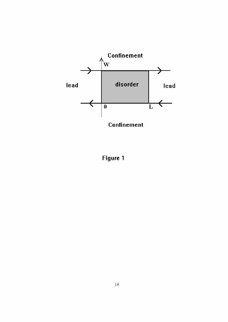
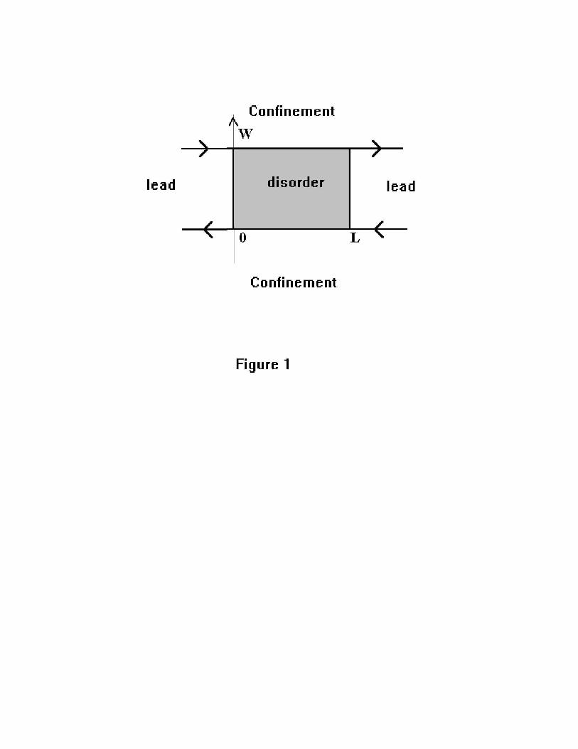
We consider the transport properties of a two-dimensional (2D) disordered strip con-nected to two disorder-free leads, as shown in figure 1. In the transverse direction, thesystem is restricted to a finite width of W by confinement potentials. The entire system issubject to a perpendicular magnetic field. In the leads the edge states are the only currentcarrying states. Therefore the problem can also be viewed as that of edge states scatteringthrough a disordered region. From the viewpoint of the Landauer-Buttiker formula [1,2],the DC transport properties are determined by the scattering matrix at the Fermi energy. Ithas been shown that the total transmission or the total back scattering of edge states leadsto the quantization of Hall conductance [3-6]; from the bulk point of view the quantizationrequires the localization of the bulk states. The equivalence between the edge state descrip-tion and the bulk point of view has generated interesting discussions [3-8]. However, therehas been no quantitative analysis as to how the edge state transmission coefficient relates tothe bulk conductivity or resistivity. It has been shown [4,5] that the longitudinal resistanceRxx of the above system is

_ Rh

where T and R are transmission and reflection coefficient of a single edge state. The followingrelation

L RhPxx = ^J7y ̂ i

has also been used in a number of articles [5,8,9], where pxx is the longitudinal resistivity,W and L are the width and length of the sample respectively. The latter relation is basedon the assumption that the resistance is a measure of the resistivity. This assumption is notjustified.

Our work is also motivated by the recent experimental and subsequent theoretical workby Shahar et al. [10,11] concerning the duality between phases on either sides of the quantumHall transitions. Using the Chalker-Coddington network model [12], we are able to obtaina previously speculated duality relation [11] for the transmission coefficient and the longi-tudinal resistance in the geometry specified above. To decide whether or not the dualityrelation explains the experiment, which was done in a different geometry, one again needsto resolve the relation between resistance and resistivity.

This paper addresses two issues. First we are concerned with the duality in the Chalker-Coddington model and how this duality manifests itself in the resistance measurement.Secondly we render a microscopic calculation for the edge state transmission coefficient inthe diffusive limit in terms of the bulk parameters, the longitudinal and Hall conductivityGXX and axy. We find a non-trivial relation between resistance and resistivity. Althoughthe calculation helps to put a restriction to the implication of the duality, it resolves anindependent issue of its own.

Section II serves as a brief review of the quantum linear response theory. There we setup the starting point for the microscopic calculations. We emphasize that for finite-sizedsystems with phase coherence, all measured quantities are conductances or resistances andare in principle sensitive to the way the measurement is set up. We make a contrast between

the bulk current density and the Landauer-Buttiker scattering point of view. In followingboth approaches in later calculations, we demonstrate their equivalence.

In section III we express the Hall and longitudinal resistance in terms of the trans-mission coefficient using the Landauer-Buttiker formula. Our derivation makes explicit theinvolvement of probes and leads in the measurement. In section IV, we proceed to discussthe duality in the discrete Chalker-Coddington model, which leads to an inverse relationfor the longitudinal resistance, but only for samples with reflection symmetry. We also lookfor the implication of the duality in the continuous limit. There the duality is between thephase with its bare Hall conductivity at <r° and the phase at n — <r° , where n is a integer.(Note: from now on we use e2/h as the unit for conductivity and h/e2 for resistivity.) Theduality relation in the continuous limit translates to a relation between the renormalizedconductivity: crxy(a^.y) + axy(n — a^.y) = n (here crxy(a^.y) denotes the renormalized axy asa function its bare value cr° ). We show that this duality relation alone is not enough toexplain the experimental claim of [10]. To do so an additional constraint between axx andaxy is required.

In section V we calculate the transmission coefficient and the resistances in the pertur-bative limit (<JXX > 1). We show that the ideal leads affect the outcome of the measurementby imposing a boundary condition on the electro-chemical potential and the Hall resistanceis thus artificially fixed to a quantized value. We find that only under the condition thatthe Hall resistivity is quantized the resistance is proportional to resistivity. The edge statescattering problem in the diffusive limit is reduced to a special boundary problem. Its an-alytical solution, by conformal mapping, is discussed in section VI. We conclude with adiscussion on the missing connections between the duality found in experiment and that inexisting models for the quantum Hall effects.

II. TWO FORMS OF THE LINEAR RESPONSE THEORY

The quantum mechanical linear response theory for non-interacting electron gas can beput in two forms. In one form one writes the local current density as a functional of theexternal field:

r ' v ( r , r ' ) £ , ( r ' ) , (2.1)

where cr^r , r') is the bilocal conductivity and can be expressed in terms of the single particleGreen's function G±(E) = 1/(E — H ± irj) where H is the single particle Hamiltonian. (Fora detailed form of <r(r, r') see [13].) The relation between the current and the external fieldis generally non-local and in the presence of magnetic field c ^ r , r') contains not only Fermisurface contribution, but also contributions from all energies below the Fermi energy.

Due to a set of current conservation constraints [13], the total current in a lead (say, thezth lead) to linear order depends only on the voltages in the leads, the VJS:

Ii = 9ijVi. (2.2)

where the conductance coefficients, the gijS, are surface integrals of <r(r, r') in the iih andjth lead:

dSi-air^-dSj. (2.3)

Although the off-Fermi-surface terms in cr(r, r') contribute to the local current response,they give zero net contribution upon surface integral [13]. As a result the g8Js can be writtenin terms of the scattering matrix at the Fermi energy. One arrives at the Landauer-Buttikerformula [1,2]

2 2

9H = jTtJ, for i + j ; gtt = &- [Ttt - N] (2.4)

where T8J is the total transmission coefficient from the iih to the jih lead,

tij is the scattering matrix between the states of the iih and the jih probe and N is the totalnumber of scattering states (or total number of edge states in the present case) at the Fermi-level. The above formula best illustrates the non-local aspect of quantum transport and hasbeen instrumental to our understanding of Anderson localization and to the formulation ofthe random matrix theory for quasi one-dimensional disorder systems. The DC conductancegij is well defined for a finite-sized disordered region (embedded in an infinite open system),therefore are good candidates for scaling analysis; moreover, they are directly measurablein experiments. However, the formula is rarely used for microscopic calculations, becauseit introduces confinements and leads which can be cumbersome to address theoretically,particularly in the presence of magnetic field. Only recently it was understood that thepresence of a confinement potential at the edges changes the boundary condition for diffusionfrom (dn)(f) = 0 to (dn + ^^-dt)p = 0 where t is the tangential and n is the normal directionof the edge [14]. The boundary condition imposed by the perfect 2D leads will be discussedin this paper.

In practice, the conductivity, a concept from classical physics, is still widely used, al-though for quantum mechanical systems it no longer bears the local interpretation. It canbe defined as the ratio between the average current density and the average field. Cautionhas to be exercised for finite-sized closed systems, where the DC dissipative conductivityaxx is zero due to the discreteness of energy levels. The DC axx is usually asymptoticallydefined from AC conductivity axx(u) by taking the system size to infinite before taking thefrequency (to) of the external field to zero. Experimentally, most of the measurements ofaxx and axy are deduced from longitudinal and Hall conductance(resistance) by extendingthe following classical relation to quantum mechanical systems:

W9xx = oxx—, gxy = axy, (2.5)

where gxx and gxy are combinations of the transmission coefficients. The "conductivities"thus defined are in fact conductances. The conductance or the transmission coefficientsdepend on a number of factors: the random scattering potential in the disordered region,the confinement potential, the property of the leads and even that of the thermal reservoirs.The result of a measurement is not independent of the way in which the measurement is

done. Without checking that the measurement results are robust against size and geometryvariations, one cannot be sure that the conductivity (or resistivity) is obtained. As we willshow in section V, even in the perturbative regimes where quantum corrections are small,Rxx and Rxy exhibit the above Ohmic type of relations only under certain conditions. Forthe critical regimes between the quantum Hall plateaus, experimental and numerical studiesfor different geometries have so far come up with a range of values for the critical value of<Jxx [15], indicating the need for a more careful study of finite-size scaling under differentboundary conditions. We would like to address this point in a future study.

III. LANDAUER-BUTTIKER FORMULA FOR RESISTANCE

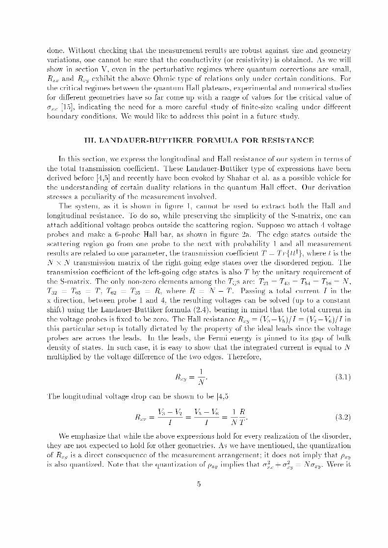
In this section, we express the longitudinal and Hall resistance of our system in terms ofthe total transmission coefficient. These Landauer-Buttiker type of expressions have beenderived before [4,5] and recently have been evoked by Shahar et al. as a possible vehicle forthe understanding of certain duality relations in the quantum Hall effect. Our derivationstresses a peculiarity of the measurement involved.

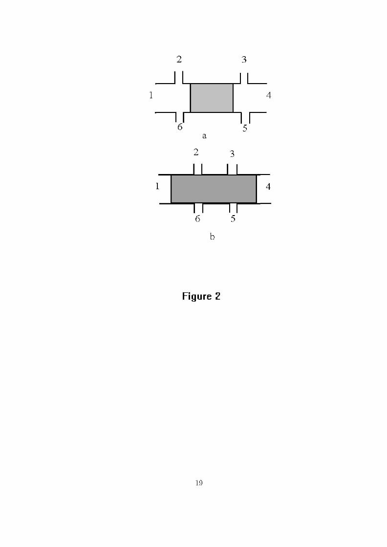
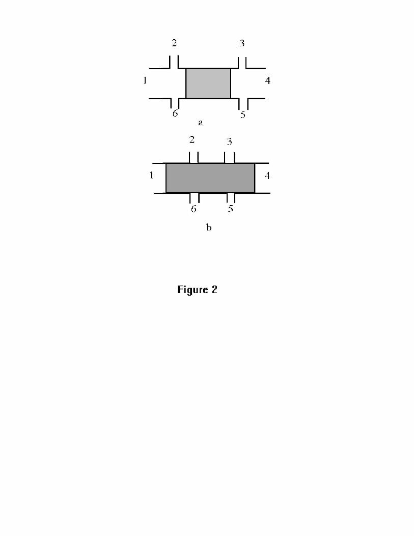
The system, as it is shown in figure 1, cannot be used to extract both the Hall andlongitudinal resistance. To do so, while preserving the simplicity of the S-matrix, one canattach additional voltage probes outside the scattering region. Suppose we attach 4 voltageprobes and make a 6-probe Hall bar, as shown in figure 2a. The edge states outside thescattering region go from one probe to the next with probability 1 and all measurementresults are related to one parameter, the transmission coefficient T = Tr{tt^}, where t is theN X N transmission matrix of the right-going edge states over the disordered region. Thetransmission coefficient of the left-going edge states is also T by the unitary requirement ofthe S-matrix. The only non-zero elements among the T8Js are: T2i = T43 = T54 = T\Q = N,T32 = T65 = T, T62 = T35 = R, where R = N — T. Passing a total current / in thex-direction, between probe 1 and 4, the resulting voltages can be solved (up to a constantshift) using the Landauer-Buttiker formula (2.4), bearing in mind that the total current inthe voltage probes is fixed to be zero. The Hall resistance Rxy = (V3 — V5)// = (V2 — Ve)/1 inthis particular setup is totally dictated by the property of the ideal leads since the voltageprobes are across the leads. In the leads, the Fermi energy is pinned to its gap of bulkdensity of states. In such case, it is easy to show that the integrated current is equal to Nmultiplied by the voltage difference of the two edges. Therefore,

_ 1xy N'

The longitudinal voltage drop can be shown to be [4,5]

Vi-V2 V5-V6 iR , , 9 ,Rxx = ; = ; = -T777T- (<3-^j

1 1 iv 1

We emphasize that while the above expressions hold for every realization of the disorder,they are not expected to hold for other geometries. As we have mentioned, the quantizationof Rxy is a direct consequence of the measurement arrangement; it does not imply that pxy

is also quantized. Note that the quantization of pxy implies that a2xx + a1 = Naxy. Were it

to be true, this would give, for critical axy = ocxy = N — 1/2, the critical axx = axx = ̂ ^—-,

which contradicts the current consensus that all integer quantum Hall transitions are thesame and that axx should be independent of N. This is one more reason why Rxx should notbe taken as axx for N > 1. (This simple measurement setup is not able to detect whetherN Landau levels are coupled by disorder or decoupled from one another in the scatteringregion, since it is only sensitive to the trace of the transmission matrix. Equilibrium amongedges states are re-enforced by the thermal reservoirs attached to the probes.)

IV. DUALITY RELATION FOR THE EDGE TRANSMISSION COEFFICIENT

Recently, studying the critical transitions between the quantum Hall plateaus, Shaharet al. [10,11] found that the longitudinal I-V curves near the critical magnetic field Bc arenon-linear and demonstrate a certain reflection symmetry with respect to the linear line atBc; more precisely, the longitudinal voltage and current appear to reverse roles at two fillingfractions, v and i/d, on either sides of the quantum Hall transition:

{Vx{u% Ix(ud)} = { / » , Vx(u)}, (4.1)

with v and ud satisfying a definite relation suggestive of charge-flux symmetry in the bosonicview of the quantum Hall effect [10,11]. The authors pointed out that duality between chargeand flux in the effective bosonic action can be the explanation of the observed relation(4.1), however there is one catch to this scenario- it requires the extra condition that thebosonic Hall resistivity remains zero across the phase transition, to which there has beenno satisfying explanation. As an alternative the same authors also suggested a fermionicscenario, appealing to the Landauer-Buttiker expression similar to (3.1) and (3.2) (theirversion is amendable to linear response). Noticing that for N = 1, Rxx goes to its inverseas T —> 1 — T = R, Shahar et al. propose that (4.1) can be explained within the Landauer-Buttiker framework if the following is true:

T(EC + AE) = 1 -T(EC- AE). (4.2)

We show that the above relation can be the consequence of certain duality embedded in theChalker-Coddington model for the quantum Hall effect. However, one can only write downthe duality relation for the transmission coefficient of a symmetric sample with L = W.

The Chalker-Coddington model [12] consists of a lattice of directed links and scatteringnodes (see figure 3), representing the semi-classical orbits along the equipotential contoursof the random potential and the tunneling among these orbits at the nodes. Each node isdescribed by a 2 X 2 scattering matrix with random phases and a fixed probability To toscatter to the right and 1 — To to the left. To is a function of the Fermi-energy. In figure3, we show one such network coupled to two edge states. At fixed Fermi energy, thereare two equivalent ways to view the network: as one built out of clockwise guiding centerorbits (the white squares) with probability 1 — To to tunnel to the neighboring orbits, orequivalently, of counter-clockwise orbits (black squares) with tunneling probability To. (AtTo = 1, the network breaks down to decoupled clockwise orbits and two edge states at thetop and bottom; at To = 0, it breaks down to decoupled counter-clockwise orbits and two

6

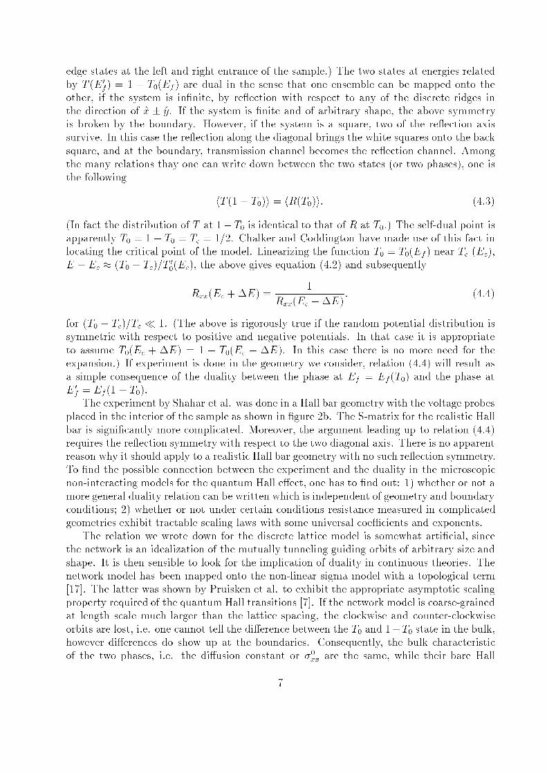
edge states at the left and right entrance of the sample.) The two states at energies relatedby T(E'j) = 1 — To(Ef) are dual in the sense that one ensemble can be mapped onto theother, if the system is infinite, by reflection with respect to any of the discrete ridges inthe direction of x ± y. If the system is finite and of arbitrary shape, the above symmetryis broken by the boundary. However, if the system is a square, two of the reflection axissurvive. In this case the reflection along the diagonal brings the white squares onto the backsquare, and at the boundary, transmission channel becomes the reflection channel. Amongthe many relations thay one can write down between the two states (or two phases), one isthe following

(T(l-T0)) = (R(T0)). (4.3)

(In fact the distribution of T at 1 — To is identical to that of R at To.) The self-dual point isapparently To = 1 — To = Tc = 1/2. Chalker and Coddington have made use of this fact inlocating the critical point of the model. Linearizing the function To = T0(Ef) near Tc (Ec),E — Ec ss (To — TC)/TQ(EC), the above gives equation (4.2) and subsequently

^ ( 4 - 4 )

for (To — Tc)/Tc <C f • (The above is rigorously true if the random potential distribution issymmetric with respect to positive and negative potentials. In that case it is appropriateto assume TO(EC + AE) = 1 — TO(EC — AE). In this case there is no more need for theexpansion.) If experiment is done in the geometry we consider, relation (4.4) will result asa simple consequence of the duality between the phase at Ej = Ej(T0) and the phase atE'f = Ef(l-T0).

The experiment by Shahar et al. was done in a Hall bar geometry with the voltage probesplaced in the interior of the sample as shown in figure 2b. The S-matrix for the realistic Hallbar is significantly more complicated. Moreover, the argument leading up to relation (4.4)requires the reflection symmetry with respect to the two diagonal axis. There is no apparentreason why it should apply to a realistic Hall bar geometry with no such reflection symmetry.To find the possible connection between the experiment and the duality in the microscopicnon-interacting models for the quantum Hall effect, one has to find out: I) whether or not amore general duality relation can be written which is independent of geometry and boundaryconditions; 2) whether or not under certain conditions resistance measured in complicatedgeometries exhibit tractable scaling laws with some universal coefficients and exponents.

The relation we wrote down for the discrete lattice model is somewhat artificial, sincethe network is an idealization of the mutually tunneling guiding orbits of arbitrary size andshape. It is then sensible to look for the implication of duality in continuous theories. Thenetwork model has been mapped onto the non-linear sigma model with a topological term[17]. The latter was shown by Pruisken et al. to exhibit the appropriate asymptotic scalingproperty required of the quantum Hall transitions [7]. If the network model is coarse-grainedat length scale much larger than the lattice spacing, the clockwise and counter-clockwiseorbits are lost, i.e. one cannot tell the difference between the To and I — To state in the bulk,however differences do show up at the boundaries. Consequently, the bulk characteristicof the two phases, i.e. the diffusion constant or a°x are the same, while their bare Hall

conductivity axy differ by one quanta. (It has been shown that the bare conductivities of

the network model are <r° = ^2 , ,T £\o and <r°, = ^2 ,,,° ^ ,2 [8,191). Since reflection is the-'o+(i--'o) xv J-o+ii—J-o) L J /

operation that maps the To phase to the 1 — To phase, we consider how the non-linear sigmamodel transforms under the one reflection operation (x —> —x or y —> —y). The topologicalterm, with axy as its coefficient, changes sign while the axx term remains the same. Since thetheory is periodic in ax , the corresponding dual phases are those parameterized by ax andn — ax , w

x , the corresponding dual phases are those parameterized by ax

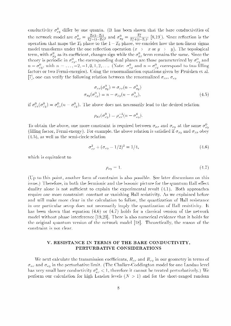
with n = . . . , —2, —1, 0,1, 2 , . . . . (Note: ax and n — ax correspond to two fillingfactors or two Fermi-energies). Using the renormalization equations given by Pruisken et al.[7], one can verify the following relation between the renormalized axx, axy

- (T°xy)

°xv{°Oxy) = n~ azy(n ~ ^xy), (4-5)

if cr° (cr°,) = <r° (n — <r°,). The above does not necessarily lead to the desired relation

To obtain the above, one more constraint is required between axx and axy at the same <r°(filling factor, Fermi energy). For example, the above relation is satisfied if axy and axx obey(4.5), as well as the semi-circle relation

°lx + K , " 1/2)2 = 1/4, (4.6)

which is equivalent to

Pxy = I- (4.7)

(Up to this point, another form of constraint is also possible. See later discussions on thisissue.) Therefore, in both the fermionic and the bosonic picture for the quantum Hall effectduality alone is not sufficient to explain the experimental result (4.1). Both approachesrequire one more constraint: constant or vanishing Hall resistivity. As we explained beforeand will make more clear in the calculation to follow, the quantization of Hall resistancein our particular setup does not necessarily imply the quantization of Hall resistivity. Ithas been shown that equation (4.6) or (4.7) holds for a classical version of the networkmodel without phase interference [19,23]. There is also numerical evidence that it holds forthe original quantum version of the network model [18]. Theoretically, the reason of theconstraint is not clear.

V. RESISTANCE IN TERMS OF THE BARE CONDUCTIVITY,PERTURBATIVE CONSIDERATIONS

We next calculate the transmission coefficients, Rxx and Rxy in our geometry in terms ofGXX and axy in the perturbative limit. (The Chalker-Coddington model for one Landau levelhas very small bare conductivity <JXX < 1, therefore it cannot be treated perturbatively.) Weperform our calculation for high Landau levels (N > 1) and for the short-ranged random

potential model, of which the bare conductivity a°x can be large. The calculation serves tostrengthen our view regarding duality in quantum Hall systems, it also has an interest of itsown, since the problem of edge state transmission in the multi-scattering, diffusive regimehas not been analyzed before. Our treatment is at most phenomenological. Its rational is asfollows. In our previous work [19], we have calculated the bilocal conductivity c r^r , r') toleading order in l/axx. We find that to leading order the non-local relation between currentj(r) and external field E(r) can be decoupled and reduced to the familiar Drude equation(with some modification to be specified later)

j , ( r ) = a ° ^ ( r ) , (5.1)

where £ = E + V/i/e is the electro motive field (/i is the local chemical potential). In thesame work we also give the generating function from which one obtains the full quantummechanical conductance. The effect of the edges can be treated within the non-linear sigmamodel, with axx and axy as the coupling constants and the presence of the topological termalters the boundary condition for diffusion. In treating the quantum mechanical system asthough it was classical, we are assuming that the field theory is renormalizable, i. e., all thequantum corrections to conductance can be accounted for by replacing the bare couplingconstants with the renormalized reversion. The assumption so far has met no contradictionat perturbative level [19]. The new ingredient is the discussion on the boundary conditionimposed by the 2D perfect leads. We show that the computation of transmission coefficientand of current distribution reduce to solving the Laplace equation with identical boundaryconditions.

In reference [19] it has been shown using the self-consistent Born approximation(SCBA)[20], which gives the leading order in l/axx, that the bilocal conductivity tensor is of thefollowing form:

-W)- S(y))\

-W)- S(y'))} d(r, r'

(5.2)

where o?(r, r') is the diffusion propagator satisfying the —V2o?(r,r') = <£(r, r'), axx, crx'yand (TI

xIy° are the SCBA version of the Streda conductivities [21,7,19]. The higher gradient

terms are of higher order in 1/L, where / is the mean free path and L is the system length.The physics implied by the leading order expression is simple. The first term, the contactterm, arises, in terms of Drude's picture for conduction, from electrons accelerating in thecombined external field E — ev X B. The second term is the diffusion term and it arisesfrom the charge density fluctuation Sne in response to the external potential, which is long-ranged. A local relation between the current and the eletromotive field can be obtained if oneintroduces an effective local chemical potential /i(r) to account for the density fluctuation[19]. However, equation (5.2) does not quite recover equation (5.1). One notices that in thediffusive term, axy splits into two parts, cr^°, which appears in the bulk diffusion current and<r^'°, which is proportional to the edge current density and shows up only at the reflecting

9

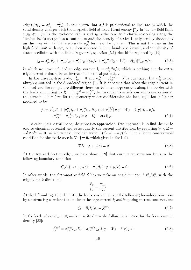
edges (axy = a1 + cr^y). It was shown that a1^ is proportional to the rate at which thetotal density changes with the magnetic field at fixed Fermi energy [7]. In the low field limit^cTo <C f (^c is the cyclotron radius and r0 is the zero field elastic scattering rate), theLandau levels merge into a continuum and the density of states is only weakly dependenton the magnetic field, therefore the a^1 term can be ignored. This is not the case in thehigh field limit with LOCT0 > I, when separate Landau bands are formed, and the density ofstates oscillates with the field. In general, equation (5.1) should be replaced by [19]

J, = *%,EV + KJ^ + v&^dvU/e + <T%°[6(y - W) - S(y)]S^ fi/e. (5.3)

in which we have included an edge current Ie = <r^'°/i/e, which is nothing but the extraedge current induced by an increase in chemical potential.

In the disorder-free leads, a1 = 0 and a^1 = cr̂ ead = N is quantized, but a^1 is notalways quantized in the disordered region [7]. It is apparent that when the edge current inthe lead and the sample are different there has to be an edge current along the border withthe leads amounting to I'e = [cl

Xyd — <r^'°]/i/e, in order to satisfy current conservation atthe corners. Therefore, for the geometry under consideration the local equation is furthermodified to be

~ w ) -

To calculate the resistance, there are two approaches. One approach is to find the staticelectro-chemical potential and subsequently the current distribution, by requiring V X E =—dH/dt = 0, in which case, one can write E(r) = — Vt^(r). The current conservationcondition for the static case is V • j = 0, which gives in the bulk

V 2 ( - ^ + /i/e) = 0. (5.5)

At the top and bottom edge, we have shown [19] that current conservation leads to thefollowing boundary condition

v®xdy(—Lp + /i/e) — a®ydx(—Lp + /i/e) = 0. (5-6)

In other words, the eletromotive field £ has to make an angle 0 = tan"1 <r° ,/cr° with the• ^-s Jb y I Jb Jb

edge along x-direction:

At the left and right border with the leads, one can derive the following boundary conditionby constructing a surface that encloses the edge current I'e and imposing current conservation:

Jx - dyre(y) = j l : a d . (5.7)

In the leads where axx = 0, one can write down the following equation for the local currentdensity [22]:

-W)- 6(y)We. (5.8)

10

Combining (5.4),(5.7) (5.8), we get

a°xxdx{-V + I'M + [ < - al:;ds]dy(-V + /i/e) = 0, (5.9)

i. e., £ has to make an angle 0' = t a n " 1 ^ , , — cr'e"d)/cr° with the border with the leads(along —y-direction ):

leadC a0 _°x _ uxy uxy

Thus the problem of finding the resistance to leading order of 1/(T°X is that of solving theLaplacian equation for the electrical chemical potential with two tilted boundary conditions.Notice that as far as the conductance or resistance is concerned, one can arrive at the correctequations by using the simpler but incorrect local relation (5.f).

Alternatively, one can follow the Landauer-Buttiker approach, i. e., one finds the trans-mission coefficient. This also requires the computation of the bilocal-conductivity tensor.For our simple geometry,

T= I dVl f dy2<Txx(rur2) (5.10)

where S\ and S2 are two the cross-sections at the left and right end of the scattering region.Making use of the SCBA expression (5.2) for c r^ r , r') , we get

x=0,x'=L

(a0)2

' W'i 0 ' W) + C/(0' 0 ' L ' 0) ~ ( / ( L ' W'i 0 ' 0) ~

In reference [19], we have shown that the diffusion propagator satisfies boundary condition(5.6) at the reflecting edges, with d replacing —if + /i/e. One can easily check that it alsosatisfies boundary condition of the form (5.9) at borders with the leads. The above expressioncan be simplified if one takes into account the additional detailed boundary condition thatthe returning probability via the incoming links is zero, the coarse-grained diffusive versionof which is d(L, 0; r) = o?(0, W; r) = 0, and the fact that transmission probability of left-goingand right-going edge states are the same, i. e., d(L, W; 0, W) = o?(0, 0; L, 0). We get

^LW;0,W) (5.12)

Defining </>(r) = 2(-^f^d(r; 0, W), </> satisfies (5.5), (5.6), (5.9) and, in addition, the fol-lowing initial condition (f)(L, 0) = 0, and </>(0, W) = N, since in the limit L —> 0, T —> N.Thus within the diffusive limit the Landauer-Buttiker approach and the current distributionapproach boil down to the same mathematical problem. Since the problem contains non-self-adjoint boundary conditions, its solution in the general case requires a special method,which we will discuss in the next section. However, some conclusions can be made beforesolving the equation.

11

Again the fact that the Hall resistance is quantized can be demonstrated usingboundary condition (5.9) alone. The current across the border with the leads is Ix =/0 dy(axx£x + axy£y) and the transverse drop in electro-chemical potential at the borders

is A(f)y = Jo dy£y(x,y)x=o:L- Making use of the relation between £x and £y from (5.9), theresult Rxy = —^ is recovered.

The next conclusion follows from the two boundary conditions. Since the field £ atthe reflecting edges and at the borders with the leads is required to point in two specificdirections, the field and current distribution is uniform only when the two directions coincide,i. e. when the bare conductivities satisfy the following constraint:

(axx)2 + ax(ax - alead) = 0, (5.13)

which is equivalent to

Xy (a0 )2 + (^0 \2 lead'\ xx J ' \ x x) xy

For (Jlxy

d = 1, the above gives the same semi-circle constraint (4.6) of Ruzin et al. Undercondition (5.13), the field distributions takes the simple form:

(7°</>o(x, y) = -E0(x + -f^y), So(x, y) = E0(x + -f^y), (5.14)

where Eo is a constant. The total current, the transverse and longitudinal electro-chemicalpotential differences can be easily calculated. Indeed RXX<SCBA = yyPxx-

The axx and axy of the Chalker-Coddington model satisfies the above. However suchbare values were computed by forcefully leaving out the quantum interference of the originalmodel [19]. Since axx < 1, the model has no perturbative regime, i. e., there does not exist alength scale within which these bare values are the leading contributions. For the Gaussianwhite noise potential model axx = (2N — l ) ^ " 1 sin2 a and ax = N — 1 + a/vr, where a isa function of the Fermi energy (we do not need its expression here, see [7]), they do notsatisfy the constraint. In this case the field and current distribution is not uniform, Rxx isnot proportional to pxx and Rxy is not equal to pxy.

As we mentioned before, the geometry we consider (figure 2a) does not correspond tothose used in the experiments, we would like to know how Rxx and Rxy change if we move thevoltage probes into the scattering region as shown in figure 2b. Assuming that the voltageprobes are very small in dimensions (much smaller than the sample length L and width W),we can treat the probes as perturbations in boundary conditions and get a rough picture bylooking at the field distribution in the main strip in the absence of these probes. If condition(5.13) is met and the field and current distribution is uniform, the electro-chemical potentialdrop transverse to the current is the same everywhere along the strip and the longitudinalpotential difference is in proportion with the distance between the probes. Such systemshave a quantized Hall resistivity, as is the case with the Chalker-Coddington network withno phase coherence or a random version of it as discussed by [23]. In the general case whenthe field is not uniform, the Hall resistance departs from the quantized value as we movethe voltage probes to the interior of the sample. However if the Hall bar is long and narrow(L ^> W), the field distribution in the interior far from the ends takes the form of equation

12

(5.14), forced by boundary condition (5.6). If the probes are placed in the region where thefield is nearly uniform, Rxx and Rxy are roughly proportional to the intrinsic p x x and p x .In this way the effect of the perfect leads is removed.

VI. ANALYTICAL SOLUTION OF THE BOUNDARY PROBLEM

To solve the boundary problem we use the method of conformal mapping, which was firstused by Girvin and Rendell [24] to find the two-probe conductance in the case of absorbingleads. The idea is as follows. Let us consider a parallelogram in the z'-plane (z1 = x' + iy'),with its top and bottom edge parallel to x'-axis and its left and right side tilted from thevertical direction by 89 = 9 —9' + 90. In this geometry, the uniform field distribution of (5.14)satisfies both boundary conditions. The solution for the rectangle geometry in the z-plane(z = x + iy) can be found if one finds a conformal mapping z' —> z which transforms theparallelogram to the rectangle. We start by writing down the complex potential 4>(z') whichcan give the correct physical field £0(x',y'). The field is related to the complex potentialthrough

— —— = by + icx.dz

It is easy to see that the following complex potential

<f>{z) = -iEoe z. (6.1)

gives £0(x.',y') in the z'-plane. The conformal transformation from z-plane to the z'-planerotates the angle at x = 0, L by 89, L, e., the rotation defined by

d-f = e'M (6.2)dz

has the boundary conditions

Im[f(z)} = 89, for x = 0, L; Im[f(z)} = 0 for y = 0, W. (6.3)

The transformation has been worked out by Girvin and Rendell to be

^ 489f(z)= V {smh[nir(z-L/2)/W]/cosh(nirL/2W)}. (6.4)

n=odd

The potential drops are:

fL

Acf)x = —E0cos(9) / dx expJo

489

, , nirLn=odd

smh[mr(x - L/2)/W}/ cosh(mrL/2W)

r-W

A(j)y = —Eosin(9 — 89) / dyexpJo

The transmission coefficient is

13

/) cos(mry/W)

(6.5)

(6.6)

(6.7)

In the limit W = L, one can show that the two integrands in (6.5) and (6.6) are equal, theexpression simplifies to be

s in( f l -M) -cos(fl')L " ^ cos0 + s i n ( 0 M ) c o s # c o s ( # ' ) '

The resistance Rxx can be obtained by either plugging the above into the Landauer-Buttikerexpression (3.2) or by calculating the total current from the field distribution, then dividingA(f)x by it.

VII. CONCLUSIONS AND DISCUSSIONS

Prompted by the experimental evidence of duality near quantum Hall transitions, weprobe the implication of duality in the Chalker-Coddington model within the fermionic non-interacting picture. For finite systems with boundaries, a duality relation holds for the edgestate transmission coefficient, however, only for a class of systems with reflection symmetry.For such systems duality leads to measurable inverse relations of the longitudinal resistanceof two states at opposite sides of a quantum Hall transition. In a general situation (forarbitrary geometry) the duality translates to a diluted version crxy(a^, ) + axy(n — <r° ) = n.Our key difference with previous authors on the subject [11] is that we think that theLandauer Buttiker argument constructed for resistance in symmetric geometry cannot beexpected to hold in other geometries, such as a Hall bar, since our calculations show thatresistance is not necessarily resistivity. If the experiment of Shahar et al. is correct and thereversal of the role of longitudinal voltage and current is indeed observed in the quantumscaling regime, it points to the possibility that the renormalized axx and axy satisfy theconstraint (4.6) first suggested by the numerical work of Ruzin et al. This has so far notbeen understood within any theoretical framework.

Our work unravels the mystery surrounding the Landauer-Buttiker argument. We per-formed a perturbative calculation for the edge state transmission coefficient in terms of theconductivities and analyze the current distribution. The presence of the 2D perfect leadsgives rise to a tilted boundary condition for diffusion, which is similar and dual to the oneat the reflecting edges, (dual in the sense that one boundary condition becomes the otheras a®y —> n — crx ) . Only when axx and axy satisfy the semi-circle constraint (equivalentto the quantization of pxy), the current distribution is uniform and the resistance RXX:Xy

is in proportion to the resistivity pXX:Xy. Our phenomenological treatment is based on ourknowledge of the bilocal conductivity cr^r, r') in the perturbative regime. To access thefinite-size scaling of the resistance in the non-perturbative critical regime, one needs to studythe form of cr,,,,(r, r') afresh.

ACKNOWLEDGMENTS

This work was based on my previous collaboration with N. Read and A. D. Stone. I alsothank A. Nersesyan for helpful comments, Z. B. Su for useful conversations, Juana Moreno

14

for a critical reading of the manuscript and the International Centre for Theoretical Physics,Trieste, for hospitality.

15

REFERENCES

[1] R. Landauer, IBM J. Res. Develop. 1, 233 (1957); R. Landauer, Phil. Mag. 21, 863(1970);M. Buttiker, Phys. Rev. Lett. 57, 1761 (1986)

[2] M. Buttiker, IBM J. Res. Develop. 32, 317 (1988).[3] B. I. Halperin, Phys. Rev. B 25, 2185 (1982).[4] P. Streda, J. Kureca and A. H. MacDonald, Phys. Rev. Lett, r 59, 1973 (1987).[5] J. K. Jain and S. A. Kivelson, Phys. Rev. Lett. 60, 1542 (1988).[6] M Buttiker, Physics Rev. B 38, 9357 (1988).[7] A. M. M. Pruisken, in The Quantum Hall Effect, edited by R.E. Prange and S.M. Girvin

(Springer-Verlag, New York, 1990), Chap. 5.[8] P. L. McEuen, A. Szafer, C. A. Richter, B. W. Alphenaar, J. K. Jain, A. D. Stone, and

R. G. Wheeler, Phys. Rev. Lett. 64, 2062 (1990).[9] Dung-Hai Lee, Ziqiang Wang and Steven Kivelson, Phys. Rev. Lett. 70, 4130 (1993).

[10] D. Shahar, D. C. Tsui, M, Shayegan, E. Shimshoni and S.L. Sondhi, Science Vol. 274,589(1996)

[11] E. Shimshoni, S. L. Sondi and D. Shahar, cond-mat 9610102, to appear in Phys. Rev.B.

[12] J. T. Chalker and P. D. Coddington, J. Phys. C 21, 2665 (1988).[13] H. U. Baranger and A. D. Stone, Phys. Rev. B 40, 8169 (1989).[14] N. Read, unpublished; D. E. Khemel'nitskii and M. Yosefin, Surface Sci. 305, 507

(1994); D. L. Maslov and D. Loss, Phys. Rev. Lett. 71, 4222 (1993)[15] Y. Huo, R. E. Hetzel, and R. N. Bhatt, Phys. Rev. Lett. 70, 481 (1993); B. M. Gammel

and W. Brenig, Phys. Rev. Lett. 73, 3286 (1994); L. P. Rokhinson, B. Su and V. J.Goldman, Solid State Communications 96, 309 (1995); Z. Wang, B. Jovanovic and D.-H. Lee, Phys. Rev. Lett. 77, 4426 (1996); D. Shahar, D. C. Tsui, M. Shayegan, R. N.Bhatt and J. E. Cunningham, Phys. Rev. Lett. 22,4511(1995).

[16] J. Kucera and P. Streda, J. Phys. C 21, 4357 (1988).[17] N. Read, unpublished; D.-H. Lee, Phys. Rev. B 50, 10788(1994); M. R. Zirnbauer, Ann.

Physik 3, 513 (1994), M. R. Zirnbauer, cond-matt/9701024.[18] A. M. Dykhne and I. M. Ruzin, Phys. Rev. B 50, 2369 (1994); I. M. Ruzin and S. Feng,

Phys. Rev. Lett. 74, 154 (1995).[19] S. Xiong, N. Read, A. D. Stone, LANL Preprint (unpublished)[20] T. Ando and Y. Uemura, J. Phys. Soc. Japan, 36, 959 (1974); T. Ando, Y. Matsumoto

and Y. Uemura, J. Phys. Soc. Japan, 39, 279 (1975).[21] L. Smrcka and P. Streda, J. Phys. C 10, 2152 (1977); P. Streda, ibid. 15, L717 (1982).[22] D. J. Thouless, Phys. Rev. Lett. 71, 1878 (1993).[23] E. Shimshoni, A. Auerbach, LANL preprint, cond-mat9607031.[24] R. W. Rendell and S. M. Girvin, Phys. Rev. B 23, 6610 (1980).

16

FIGURES

FIG. 1. Edge states scattering through a disordered region.

FIG. 2. The Hall bar geometry, a: fictitious version with the voltage probes set outside thedisordered region, b: more realistic version with the voltage probes set in the interior of the sample.

FIG. 3. Duality in the Chalker-Coddington network model for the quantum Hall effect. Atfixed Fermi energy Ej, the system can be viewed as a network built of counter-clockwise orbitsenclosing the shaded areas with tunneling probability 1 — To(Ef), or equivalently, a network builtof clockwise orbits enclosing the white regions with tunneling probability To(Ef). The phase atTo(Ef) can be mapped onto the phase at To(E'r) = 1 — To(Ef) upon reflection with respect to oneof the diagonal axis.

17

lead

Jf

\

?

/\

. Confinement

disorder

0 L

\?

lead

Confinement

Figure 1

18

b

Figure 2

19

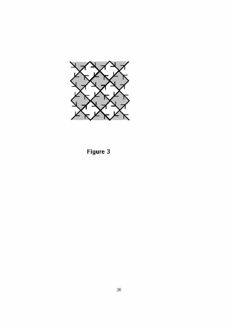
Figure 3

20

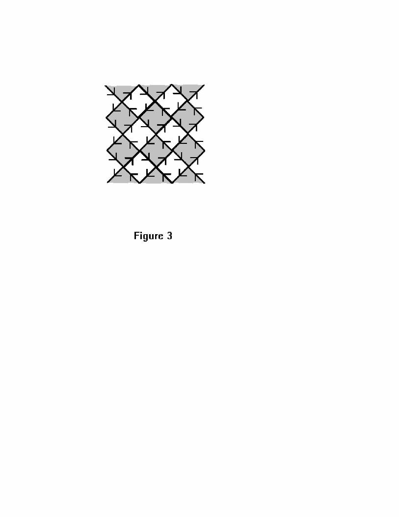
Figure 3

b

Figure 2

Confinement

W

lead lead

Confinement

Figure 1