edge detection and ridge detection with automatic scale...
TRANSCRIPT
Edge detection and ridge detection
with automatic scale selection
Tony Lindeberg
Computational Vision and Active Perception Laboratory (CVAP)Department of Numerical Analysis and Computing Science
KTH (Royal Institute of Technology)S-100 44 Stockholm, Sweden.
http://www.nada.kth.se/˜tonyEmail: [email protected]
Technical report ISRN KTH/NA/P–96/06–SE, May 1996, Revised August 1998.Int. J. of Computer Vision, vol 30, number 2, 1998. (In press).Shortened version in Proc. CVPR’96, San Francisco, June 1996.
Abstract
When computing descriptors of image data, the type of information that can beextracted may be strongly dependent on the scales at which the image operatorsare applied. This article presents a systematic methodology for addressing thisproblem. A mechanism is presented for automatic selection of scale levels whendetecting one-dimensional image features, such as edges and ridges.
A novel concept of a scale-space edge is introduced, defined as a connectedset of points in scale-space at which: (i) the gradient magnitude assumes a localmaximum in the gradient direction, and (ii) a normalized measure of the strengthof the edge response is locally maximal over scales. An important consequenceof this definition is that it allows the scale levels to vary along the edge.
Two specific measures of edge strength are analysed in detail, the gradientmagnitude and a differential expression derived from the third-order derivativein the gradient direction. For a certain way of normalizing these differential de-scriptors, by expressing them in terms of so-called γ-normalized derivatives, animmediate consequence of this definition is that the edge detector will adapt itsscale levels to the local image structure. Specifically, sharp edges will be detectedat fine scales so as to reduce the shape distortions due to scale-space smoothing,whereas sufficiently coarse scales will be selected at diffuse edges, such that anedge model is a valid abstraction of the intensity profile across the edge.
Since the scale-space edge is defined from the intersection of two zero-crossingsurfaces in scale-space, the edges will by definition form closed curves. This sim-plifies selection of salient edges, and a novel significance measure is proposed,by integrating the edge strength along the edge. Moreover, the scale informationassociated with each edge provides useful clues to the physical nature of the edge.
With just slight modifications, similar ideas can be used for formulating ridgedetectors with automatic selection, having the characteristic property that theselected scales on a scale-space ridge instead reflect the width of the ridge.
It is shown how the methodology can be implemented in terms of straightfor-ward visual front-end operations, and the validity of the approach is supportedby theoretical analysis as well as experiments on real-world and synthetic data.
Keywords: edge detection, ridge detection, scale selection, diffuseness, normalizedderivative, Gaussian derivative, scale-space, multi-scale representation, featuredetection, computer vision
i

ii Lindeberg
Contents
1 Introduction 1
2 The need for automatic scale selection in edge detection 3
3 Scale-space and automatic scale selection: Review 6
3.1 Scale-space representation . . . . . . . . . . . . . . . . . . . . . . . . . . . . . 63.2 Scale selection from maxima over scales of normalized derivatives . . . . . . . 7
4 Edge detection with automatic scale selection 8
4.1 Local directional derivatives . . . . . . . . . . . . . . . . . . . . . . . . . . . . 84.2 Differential geometric edge definition . . . . . . . . . . . . . . . . . . . . . . . 84.3 Scale selection: Selection of edge curves on the edge surface . . . . . . . . . . 94.4 Derivatives of edge strength with respect to scale . . . . . . . . . . . . . . . . 104.5 Theoretical analysis for characteristic model signals . . . . . . . . . . . . . . . 104.6 Measure of edge saliency . . . . . . . . . . . . . . . . . . . . . . . . . . . . . . 144.7 Experiments . . . . . . . . . . . . . . . . . . . . . . . . . . . . . . . . . . . . . 154.8 Summary . . . . . . . . . . . . . . . . . . . . . . . . . . . . . . . . . . . . . . 22
5 Ridge detection with automatic scale selection 22
5.1 Local directional derivatives . . . . . . . . . . . . . . . . . . . . . . . . . . . . 235.2 Differential geometric ridge definition . . . . . . . . . . . . . . . . . . . . . . . 235.3 The need for automatic scale selection in ridge detection . . . . . . . . . . . . 255.4 Scale selection: Selection of ridge curves on the ridge surface . . . . . . . . . . 255.5 Measures of ridge strength . . . . . . . . . . . . . . . . . . . . . . . . . . . . . 265.6 Qualitative properties of different ridge strength measures . . . . . . . . . . . 265.7 Experiments . . . . . . . . . . . . . . . . . . . . . . . . . . . . . . . . . . . . . 305.8 Summary . . . . . . . . . . . . . . . . . . . . . . . . . . . . . . . . . . . . . . 30
6 Relations to previous works 34
7 Summary and discussion 35
7.1 Edge detection with automatic scale selection . . . . . . . . . . . . . . . . . . 357.2 Ridge detection with automatic scale selection . . . . . . . . . . . . . . . . . . 367.3 Scale-space derivatives of high order . . . . . . . . . . . . . . . . . . . . . . . 36
8 Extensions and further work 36
8.1 Multiple feature responses at different scales . . . . . . . . . . . . . . . . . . . 368.2 Selective mechanisms . . . . . . . . . . . . . . . . . . . . . . . . . . . . . . . . 378.3 Alternative approaches to feature detection . . . . . . . . . . . . . . . . . . . 37
9 Conclusion: Principles for scale selection 38
A Appendix: Derivatives of edge strength with respect to scale 39
A.1 Derivatives of Gγ−normL with respect to scale . . . . . . . . . . . . . . . . . . 39A.2 Derivatives of Tγ−normL with respect to scale . . . . . . . . . . . . . . . . . . 39
B Appendix: Derivatives of ridge strength with respect to scale 40
C Appendix: Detailed algorithmic description 42
C.1 Pre-processing: Computation of differential invariants . . . . . . . . . . . . . 42C.2 Tracking the intersection of the zero-crossing surfaces . . . . . . . . . . . . . 42

Edge detection and ridge detection with automatic scale selection 1
1 Introduction
One of the most intensively studied subproblems in computer vision concerns howto detect edges from grey-level images. The importance of edge information for earlymachine vision is usually motivated from the observation that under rather generalassumptions about the image formation process, a discontinuity in image brightnesscan be assumed to correspond to a discontinuity in either depth, surface orientation,reflectance or illumination. In this respect, edges in the image domain constitute astrong link to physical properties of the world. A representation of image informationin terms of edges is also compact in the sense that the two-dimensional image patternis represented by a set of one-dimensional curves. For these reasons, edges have beenused as main features in a large number of computer vision algorithms.
A non-trivial aspect of edge based analysis of image data, however, concerns whatshould be meant by a discontinuity in image brightness. Real-world image data areinherently discrete, and for a function defined on a discrete domain, there is no naturalnotion of “discontinuity”. This means that there is no inherent way to judge whatare the edges in a given discrete image. Therefore, the concept of an image edge isonly what we define it to be.
From this viewpoint, it is easy to understand that a large number of approacheshave been developed for detecting edges. The earliest schemes focused on the detec-tion of points at which the gradient magnitude is high. Derivative approximationswere computed either from the pixels directly, using operators such as Robert’s crossoperator (Roberts 1965), the Sobel operator (Pingle 1969) and the Prewitt opera-tor (Prewitt 1970), or from local least-squares fitting (Haralick 1984). An importantstep was then taken by the introduction of multi-scale techniques. (Torre and Poggio1980) motivated the need for linear filtering as a pre-processing step to differenti-ation, in order to regularize ill-posed differentiation into well-posed operators. TheMarr-Hildreth operator (Marr and Hildreth 1980) was motivated by the rotationalsymmetry of the Laplacian operator and the special property of the Gaussian kernelas being the only real function that minimizes the product of the variances of the filterin the spatial and the Fourier domains.1 Other early techniques with a multi-scalecharacter were presented by (Rosenfeld and Thurston 1971) and by (Marr 1976).
(Canny 1986) considered the problem of determining an “optimal smoothing fil-ter” of finite support for detecting step edges. The methodology was to maximize acertain performance measure constituting a trade-off between detection and localiza-tion properties given a restriction on the probability of obtaining multiple responsesto a single edge. He also showed that the resulting smoothing filter could be wellapproximated by the first-order derivative of a Gaussian kernel. (Deriche 1987) ex-tended this approach to filters with infinite support, and proposed a computationallyefficient implementation using recursive filters.2 (Canny 1986) also introduced thenotions of non-maximum suppression and hysteresis thresholding. Similar conceptswere developed independently by (Korn 1988).
These ideas have then been furthered by several authors, and a large literaturehas evolved on the design of “optimal edge detectors” for different types of edgemodels, noise models, and optimality criteria, see, for example, (Nalwa and Binford
1As is well-known, however, this operator gives poor localization at curved structures, and containsno mechanism for distinguishing “false” from “true” edges.
2In two dimensions, however, such recursive filters may be strongly biased to the orientation ofimage grid.

2 Lindeberg
1986; Boyer and Sarkar 1991; Petrou and Kittler 1991; Wilson and Bhalerao 1992).3
Another subject, which has been given large attention during recent years, is thereplacement of the linear smoothing operation by a non-linear smoothing step, withthe goal of avoiding smoothing across object boundaries, see (Perona and Malik 1990;Saint-Marc et al. 1991; Nitzberg and Shiota 1992; Haar Romeny 1994) for examples.
A trade-off problem, which is common for all these edge detection schemes, and,in fact, arises for any multi-scale feature detector, concerns how much smoothing touse in the smoothing step. A larger amount of smoothing will, in general, have thedesirable effect of increasing the suppression of noise and other interfering fine-scalestructures. This, in turn, can be expected to simplify the detection problem at thecost of possible poor localization. A smaller amount of smoothing, on the other hand,can be expected to improve the localization properties at the cost of a lower signal-to-noise ratio. To circumvent this problem, (Bergholm 1987) proposed to detect edges atcoarse scales, and to follow these to finer scales using edge focusing. He did, however,not present any method for determining the scale level for the detection step, or towhat scales the edges should be localized. Hence, edge focusing serves mainly as aselection procedure, which among all the edges at the finer (localization) scale selectsthose who can be traced to corresponding edges at the coarser (detection) scale.
The subject of this article is to address the general problem of automaticallyselecting local appropriate scales for detecting edges in a given data set. As will beillustrated by examples later in section 4, the choice of scale levels can crucially affectthe result of edge detection. Moreover, different scale levels will, in general, be neededin different parts of the image. Specifically, coarse scale levels are usually necessaryto capture diffuse edges, due to shadows and other illumination phenomena.
To cope with this problem, we will propose an extension of the notion of non-maximum suppression, with the scale dimension included already in the edge defini-tion. This approach builds upon previous work on feature detection with automaticscale selection (Lindeberg 1993c, 1994a), based on the idea that in the absence offurther evidence, scale levels for feature detection can be selected from the scales atwhich normalized measures of feature strength assumes local maxima over scales. Itwill be shown that for two specific measures of edge strength, an immediate conse-quence of this definition is that fine scale levels will be (automatically) selected forsharp edges, and coarse scales for diffuse edges.
In addition, an edge detector based on this approach computes a diffuseness esti-mate at each edge point. Such attribute information constitutes an important cue tothe physical nature of the edge. Another important property of this approach is thatthe scale levels are allowed to vary along the edge, which is essential to capture edgesfor which the degree of diffuseness varies along the edge.
In this respect, the approach we will arrive at will have certain properties in com-mon with methods for estimating edge diffuseness (Mallat and Zhong 1992; Zhangand Bergholm 1993). With just a slight modification, it can also be used for formu-lating ridge detection methods with automatic scale selection. Let use, however, deferfrom discussing these relationships until we have described our own methodology. Thepresentation begins with a hands-on demonstration of the need for a scale selectionmechanism in edge detection. After this, a more detailed outline will be given of howthe article is organized.
3An important aspect to keep in mind concerning such “optimal edge detectors”, however, is thatthe optimality is relative to the model, and not necessarily with respect to the performance of theedge detector when applied to real-world data.

Edge detection and ridge detection with automatic scale selection 3
2 The need for automatic scale selection in edge detection
To illustrate the need for an explicit mechanism for automatic scale selection whendetecting edges from image data about which no a priori information is available, letus consider the effects of performing edge detection on image data at different scales.
Figure 1 shows the result of applying a standard edge detector (Lindeberg 1993b)4
to two images, which have been smoothed by convolution with Gaussian kernelsof different widths. (To isolate the behaviour of the edge detector, no thresholdinghas been performed on the gradient magnitude.) As can be seen, different types ofedge structures give rise to edge curves at different scales. In the left image of theoffice scene, the sharp edges due to object boundaries give rise to connected edgesegments at both fine and coarse scales. For these edges, the localization is best atfine scales, since an increased amount of smoothing mainly results in destructiveshape distortions. At the finest scales, however, there is a large number of otheredge responses due to noise and other spurious structures. Moreover, the diffuse edgestructures fail to give rise to connected edge curves at the finest scales. Hence, coarserscale levels are necessary to capture the shadow edges (as well as other edge diffuseedge structures). This effect is even more pronounced for the synthetic fractal imagein the right column, for which it can be clearly seen how the edge detector respondsto qualitatively different types of edge structures at different scales.
Figure 2 shows a further example of this behaviour for an image of an arm, withand without 10 % added white Gaussian noise. Here, it can be clearly seen that thesharp edge structures (the outline of the arm and the boundaries of the table) giverise to edge curve responses both at fine and coarse scales, whereas the diffuse edgestructures (the shadow on the arm, the cast shadow on the table, and the reflection ofthe hand on the table) only give rise to connected edge curves only at coarser scales.When noise is added (the images in the right column), the diffuse edges are muchmore sensitive to these local perturbations than the sharp edges. Furthermore, if asmuch smoothing is applied to the cast shadow on the table as is necessary to capturethe widest parts of its boundaries as closed edge curves, the shape distortions willbe substantial near the fingertip. Hence, to capture this shadow with a reasonablytrade-off between detection and localization properties, we must allow the amount ofsmoothing to vary along the edge.
In summary, these experiments illustrate how an edge detector responds to differ-ent types of edge structures in qualitatively different ways depending on the physicalnature of the edge and the scale level at which the edge detector operates. A naturalrequirement on any edge detector intended to work robustly in a complex unknownenvironment is that it must be able to make these qualitatively different types ofbehaviours explicit for further processes. Whereas a straightforward approach couldbe to detect edges at multiple scales, and then send these as input to higher-levelprocessing modules, such a representation would not only be highly redundant. Itmay also be very hard to interpret, since the representation of the edge behaviour isonly implicit. For this reason, and in view of the fact that the choice of scale levelscrucially affects the performance of the edge detector, (and different scale levels will,in general, be required in different parts of the image), we argue that it is essentialthat the edge detection module is complemented by an explicit mechanism whichautomatically adapts the scale levels to the local image structure.5
4This specific implementation of non-maximum suppression expressed in a scale-space setting willbe described in more detail in section 4.2.
5Concerning the common use of a single fixed (often rather fine) scale level for edge detection in

4 Lindeberg
Scale-space representation Edges Scale-space representation Edges
t = 1.0
t = 4.0
t = 16.0
t = 64.0
t = 256.0
Figure 1: Edges computed at different scales from an image of an indoor office scene anda synthetic fractal image. Observe how different types of edge structures are extracted atdifferent scales, and specifically how certain diffuse edge structures fail to give rise to connectededge curves at the finest levels of scale. (Image size: 256*256 and 182*182 pixels.)

Edge detection and ridge detection with automatic scale selection 5
Scale-space representation Edges Scale-space representation Edges
t = 1.0
t = 4.0
t = 16.0
t = 64.0
t = 256.0
Figure 2: Edges computed at different scales from an image of arm. The left column showsresults computed from the original image, and the right column corresponding results afteradding 10 % white Gaussian noise to the raw grey-level image. (Image size: 256*256 pixels.)
6 Lindeberg
The requirements on such a mechanism are (i) to output a more compact repre-sentation of the edge information than a raw multi-scale edge representation, and (ii)to produce edge curves with an appropriate trade-off between detection and localiza-tion properties. Specifically, some of the desirable properties of this mechanism are todetect sharp edges at sufficiently fine scales so as to minimize the negative influenceof the smoothing operation. For diffuse edges, the scale selection mechanism shouldselect sufficiently coarse scales, such that a smooth edge model is a valid abstractionof the local intensity variations. Moreover, to capture edges with variable degree ofdiffuseness, it will in general be necessary to allow the scale levels to vary along theedge. The main subject of this article is to develop a framework for edge detection,in which the scale dimension is take into account already the edge definition, and theabovementioned properties follow as consequences of the proposed definitions.
The presentation is organized as follows: Section 3 reviews some of the mainresults of scale-space theory as well as the main steps in a general methodologyfor automatic scale selection developed in (Lindeberg 1993c, 1994a). In section 4,this methodology is adapted to the edge detection problem. It is shown how thenotion of non-maximum suppression can be extended to the scale dimension, bymaximizing a suitable measure of edge strength over scales. A theoretical analysisof the behaviour of the resulting scale selection method is presented for a numberof characteristic edge models. Experimental results are also presented for differenttypes of real-world and synthetic images. Then, section 5 shows how these ideas, in aslightly modified version, can be applied to the ridge detection problem, and be usedfor formulating a ridge detector with automatic scale selection. Section 6 explainsthe relations to previous works on these subjects, and section 7 summarizes the mainproperties of the proposed approach. Finally, section 8 outlines natural extensions ofthis methodology, and section 9 concludes with the implications of this work withrespect to the previously proposed scale selection principle.
3 Scale-space and automatic scale selection: Review
3.1 Scale-space representation
A fundamental problem that arises whenever computing descriptors from image dataconcerns what image operators to use. A systematic approach that has been developedfor dealing with this problem is provided scale-space theory (Witkin 1983; Koenderink1984; Yuille and Poggio 1986; Lindeberg 1990, 1994c; Florack et al. 1992). It focuseson the basic fact that image structures, like objects in the world, exist as meaningfulentities over certain ranges of scale, and that one, in general, cannot expect to knowin advance what scales are appropriate for describing those.
The essence of the results from scale-space theory is that if one assumes thatthe first stages of visual processing should be as uncommitted as possible, and haveno particular bias, then convolution with Gaussian kernels and their derivatives ofdifferent widths is singled out as a canonical class of low-level operators. Hence, given
many computer vision applications, let us point out that such a strategy may be sufficient for scenesthat are sufficiently simple, and the external conditions are under sufficiently good control, such thatthe contrast between the interesting objects and the background is high, and the edge structures aresharp. For such data, a large range of scales can often be used for extracting connected edge curves,and any scale in that range may therefore be an acceptable choice. The complications we want toaddress in this paper are those arising when a single scale is not sufficient and/or such a scale cannotbe not known in advance. Note that (unlike sometimes implicitly assumed in previous works) thesetypes of problems are not eliminated by a coarse-to-fine approach.

Edge detection and ridge detection with automatic scale selection 7
any image f : R2× → R, its scale-space representation L : R
2 ×R+ → R is defined by
L(.; t) = g(.; t) ∗ f (1)
where g : R2 × R+ → R denotes the Gaussian kernel given by
g(x; t) =1
2πte−(x2+y2)/(2t). (2)
and t is the scale parameter. From this representation, scale-space derivatives arethen defined by
Lxαyβ (·; t) = ∂xαyβL(·; t) = gxαyβ(·; t) ∗ f, (3)
where (α, β) denotes the order of differentiation. The output from these operatorscan be used as a basis for expressing a large number of visual operations, such as fea-ture detection, matching, and computation of shape cues. A particularly convenientframework for expressing these is in terms of multi-scale differential invariants (Koen-derink and van Doorn 1992; Florack et al. 1992), or more specifically, as singularities(maxima or zero-crossings) of such entities (Lindeberg 1993b).
3.2 Scale selection from maxima over scales of normalized derivatives
A basic problem that arises for any such feature detection method expressed withina multi-scale framework concerns how to determine at what scales the image fea-tures should be extracted, or if the feature detection is performed at several scalessimultaneously, what image features should be regarded as significant.
Early work addressing this problem for blob-like image structures was presentedin (Lindeberg 1991, 1993a). The basic idea was to study the behaviour of imagestructures over scales, and to measure saliency from the stability of image structuresacross scales. Scale levels were, in turn, selected from the scales at a certain normalizedblob measure assumed local maxima over scales.
Then, in (Lindeberg 1993c, 1994a) an extension was presented to other aspects ofimage structure. A general heuristic principle was proposed stating that local maximaover scales of (possibly non-linear) combinations of normalized derivatives,
∂ξ =√
t ∂x, (4)
serve as useful indicators reflecting the spatial extent of corresponding image struc-tures. It was suggested that this idea could be used as a major guide for scale selectionalgorithms, which automatically adapt the local scale of processing to the local im-age structure. Specifically, it was proposed that feature detection algorithms withautomatic scale selection could be formulated in this way. Integrated algorithms werepresented, applying this idea to blob detection and corner detection with automaticscale selection, and early results were shown for the edge detection problem.
In this article, we shall develop more generally how this scale selection princi-ple applies to the detection of one-dimensional image features, such as edges andridges. For reasons that will become apparent later, we shall also extend the notionof normalized derivatives, and introduce a γ-parameterized normalized derivative by
∂x,γ−norm = tγ/2 ∂x. (5)
When γ = 1, this definition is identical to the previous notion of normalized derivativein (4). As we shall see in section 4.5 and section 5.6, however, the additional degree offreedom in the parameter γ will be essential when formulating scale selection mech-anisms for detecting one-dimensional features such as edges and ridges.
8 Lindeberg
4 Edge detection with automatic scale selection
In this section, we shall first review basic notions when expressing a differential ge-ometric edge detector in terms of local directional derivatives. Then, we turn to theproblem of formulating a mechanism for automatic scale selection, and illustrate itsperformance by theoretical analysis and experiments.
4.1 Local directional derivatives
A convenient framework to use when computing image features from differential in-variants, is to define the feature descriptors in terms of local directional derivativesrelative to some preferred coordinate system. A natural way to construct such a sys-tem suitable for edge detection is as follows: At any point (x0, y0) in a two-dimensionalimage, introduce a local coordinate system (u, v) with the v-axis parallel to the gra-dient direction at (x0, y0) and the u-direction perpendicular, i.e.,
(
cos αsinα
)
=1
√
L2x + L2
y
(
Lx
Ly
)
∣
∣
∣
∣
∣
∣
(x0,y0)
. (6)
Directional derivatives in this local (u, v)-system are related to partial derivatives inthe Cartesian coordinate system by
∂u = sinα ∂x − cos α ∂y, ∂v = cos α ∂x + sin α∂y, (7)
and the (u, v)-system is characterized by the fact that one of the two first-orderderivatives, Lu, is zero.
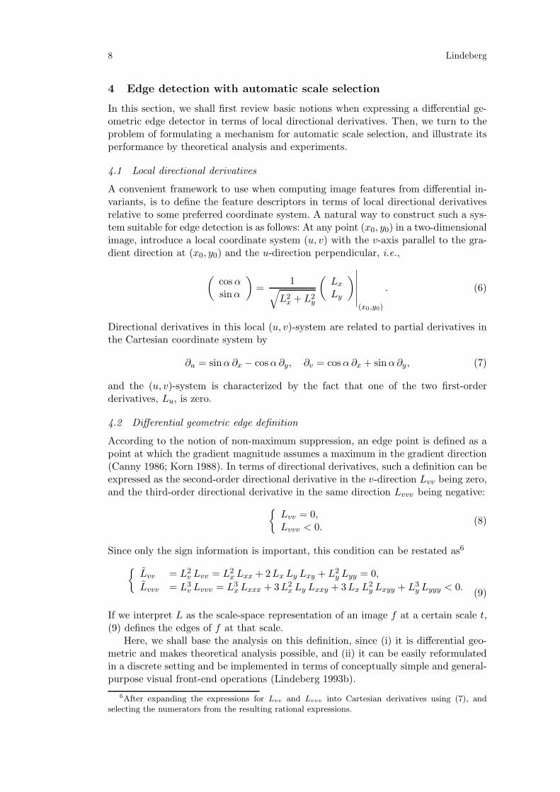
4.2 Differential geometric edge definition
According to the notion of non-maximum suppression, an edge point is defined as apoint at which the gradient magnitude assumes a maximum in the gradient direction(Canny 1986; Korn 1988). In terms of directional derivatives, such a definition can beexpressed as the second-order directional derivative in the v-direction Lvv being zero,and the third-order directional derivative in the same direction Lvvv being negative:
{
Lvv = 0,Lvvv < 0.
(8)
Since only the sign information is important, this condition can be restated as6
{
Lvv = L2v Lvv = L2
x Lxx + 2Lx Ly Lxy + L2y Lyy = 0,
Lvvv = L3v Lvvv = L3
x Lxxx + 3L2x Ly Lxxy + 3Lx L2
y Lxyy + L3y Lyyy < 0.
(9)
If we interpret L as the scale-space representation of an image f at a certain scale t,(9) defines the edges of f at that scale.
Here, we shall base the analysis on this definition, since (i) it is differential geo-metric and makes theoretical analysis possible, and (ii) it can be easily reformulatedin a discrete setting and be implemented in terms of conceptually simple and general-purpose visual front-end operations (Lindeberg 1993b).
6After expanding the expressions for Lvv and Lvvv into Cartesian derivatives using (7), andselecting the numerators from the resulting rational expressions.
Edge detection and ridge detection with automatic scale selection 9
4.3 Scale selection: Selection of edge curves on the edge surface
If the edge definition (8) is applied at all scales in the scale-space representation ofan image, the edge curves will sweep out a surface in scale-space. This surface will bereferred to as the edge surface in scale-space.
In view of the scale selection principle reviewed in section 3.2, a natural extensionof the notion of non-maximum suppression is to define an edge as a curve on the edgesurface in scale-space such that some suitably selected measure of edge strength islocally maximal with respect to scale on this curve. Thus, given such a (normalized)measure of edge strength EnormL, let us define a scale-space edge as the intersectionof the edge surface in scale-space with the surface defined by EnormL being maximalover scales. In differential geometric terms, this scale-space edge is thus defined as aconnected set of points {(x, y; t) ∈ R
2 × R+} (a curve Γ) which satisfies
{
∂t(EnormL(x, y; t)) = 0,∂tt(EnormL(x, y; t)) < 0,
{
Lvv(x, y; t) = 0,Lvvv(x, y; t) < 0.
(10)
Of course, there are several possible ways of expressing the notion that EnormL shouldassume local maxima over scales on the edge curve. In (10), this condition is formu-lated as zero-crossings of the partial derivative of EnormL with respect to the scaleparameter (i.e., a directional derivative in the vertical scale direction). A natural al-ternative is to consider directional derivatives in a direction in the tangent plane tothe edge surface, and to choose this direction as the steepest ascent direction of thescale parameter. In other words, let
N = (Nx, Ny, Nt) = ∇(x,y; t)(EnormL)∣
∣
P0= (∂x(EnormL), ∂y(EnormL), ∂t(EnormL))
denote the (unnormalized) normal direction of the edge surface in scale-space, anddefine the (normalized) steepest ascent direction of the scale parameter by
T = (Tx, Ty, Tt) =(−Nx Nt, −Ny Nt, N2
x + N2y )
√
(N2x + N2
y ) (N2x + N2
y + N2t )
. (11)
Then, with the directional derivative operator in the T -direction,
∂T = Tx ∂x + Ty ∂y + Tt ∂t, (12)
an alternative definition of a scale-space edge is as a connected set of points Γ ={(x, y; t) ∈ R
2 × R+} that satisfies
{
∂T (EnormL(x, y; t)) = 0,∂TT (EnormL(x, y; t)) < 0,
{
Lvv(x, y; t) = 0,Lvvv(x, y; t) < 0.
(13)
The general scale selection method we propose for edges (and more generally alsofor other one-dimensional features), is to extract the features from the intersectionbetween the feature surface in scale-space with the surface defined by a measure of(normalized) feature strength being locally maximal with respect to scale.
What remains to turn this idea into an operationally useful definition for detect-ing edges is to define the measure of edge strength. Based on the γ-parameterizednormalized derivative concept introduced in (5), we shall here consider the following
10 Lindeberg
two γ-normalized differential entities:
Gγ−normL = L2v,γ−norm
= tγ (L2x + L2
y), (14)
Tγ−normL = −Lvvv,γ−norm
= −t3 γ (L3x Lxxx + 3L2
x Ly Lxxy + 3Lx L2y Lxyy + L3
y Lyyy).(15)
The first entity, the gradient magnitude, is the presumably simplest measure of edgestrength to think of in edge detection. (Here, we have have squared it to simplify thedifferentiations to be performed in next section.). The second entity originates fromthe sign condition in the edge definition (9). As we shall see later, both these strengthmeasures are useful in practice, but have slightly different properties.
4.4 Derivatives of edge strength with respect to scale
In the definition of scale-space edge, expressions such as ∂t(EnormL) and ∂tt(EnormL)occur. In this section, we shall present a methodology for rewriting such differentialexpressions involving derivatives of the scale-space representation with respect to thescale parameter in terms of spatial derivatives only.
Since the scale-space representation L satisfies the diffusion equation, the spatialderivatives of L satisfy this equation as well. This implies that we can trade derivativeswith respect to the scale parameter by spatial derivatives according to
∂t(Lxαyβ ) =1
2∇2
(x,y)(Lxαyβ ) =1
2(Lxα+2yβ + Lxαyβ+2). (16)
In appendix A.1 and appendix A.2, this idea is applied to the first- and second-orderderivatives of Gγ−normL and Tγ−normL with respect to the scale parameter. Notethat the differential expressions obtained contain spatial derivatives of L up to orderthree and five concerning Gγ−normL, and spatial derivatives of L up to order five andseven concerning Tγ−normL. Whereas one could raise a certain scepticism concerningthe applicability of derivatives of such high order to real-world image data, we shallin section 4.7 demonstrate that these descriptors can indeed be used for computinghighly useful edge features, when integrated into a scale selection mechanism.
Before turning to experiments, however, let us first investigate the properties ofthe proposed scale selection method theoretically.
4.5 Theoretical analysis for characteristic model signals
To understand the consequences of using local maxima over scales of Gγ−normL andTγ−normL for selecting scale levels for edge detection, we shall in this section analysea set of characteristic model signals, for which a closed-form analysis is tractable.
4.5.1 Diffuse Gaussian step edge
Consider first a diffuse Gaussian step edge, defined as the primitive function of aGaussian kernel,
ft0(x, y) = Φ(x; t0) =
∫ x
x′=−∞g(x′; t0) dx′. (17)

Edge detection and ridge detection with automatic scale selection 11
Here, g denotes the one-dimensional Gaussian kernel g(x; t) = 1√2πt
e−x2/(2t), and t0represents the degree of diffuseness of the edge. From the semi-group property of theGaussian kernel, it follows that the scale-space representation of this signal is
L(x, y; t) = Φ(x; t0 + t) =
∫ x
x′=−∞g(x′; t0 + t) dx′. (18)
On the edge, i.e. at x = 0, the γ-normalized first-order derivative is
tγ/2 Lx(0, y; t) = tγ/2 g(x; t0 + t)∣
∣
∣
x=0=
1√2π
tγ/2
(t0 + t)1/2, (19)
and the γ-normalized third-order derivative
t3γ/2 Lxxx(0, y; t) = tγ/2 (x2 − t − t0)
(t + t0)2g(x; t0 + t)
∣
∣
∣
∣
x=0
= − 1√2π
t3γ/2
(t0 + t)3/2.(20)
Scale selection based on Gγ−normL: By differentiating the first-order measure of edgestrength
∂t((Gγ−normL)(0, y; t)) = ∂t(tγ L2
x(0, y; t))
∼ ∂t
(
tγ
t0 + t
)
=tγ−1
(t0 + t)2(γ t0 − (1 − γ) t), (21)
we see that when 0 < γ < 1 this measure assumes a unique maximum7 over scales at
tGγ−norm=
γ
1 − γt0. (22)
Requiring the maximum to be assumed at tGγ−norm= t0 gives γ = 1
2 . If we then insert(22) into (19) we see that the edge strength measure at the selected scale is given by
Lξ(0, y; tGγ−norm) =
1
2√
πt−(1−γ)/20 (23)
Scale selection based on Tγ−normL: For the third-order measure of edge strength,the γ-normalized magnitude is proportional to the third power of Gγ−normL:
(Gγ−normL)(0, y; t) = −t3γ L3x(0, y; t)Lxxx(0, y; t) ∼
(
tγ
t0 + t
)3
. (24)
Hence, for this edge model, the two scale selection methods have the same effect.
7For the singular boundary case γ = 0, corresponding to no derivative normalization, the monotonedecrease of edge strength with scale is consistent with the general smoothing effect of the diffusionequation, which means that the amplitude of local variations decreases. In the other boundary caseγ = 1, corresponding to traditional derivative normalization according to (4), the edge strengthincreases monotonically with scale, and asymptotically approaches the height of the diffuse step edge.A scale selection method based on such derivative normalization, would thus select an infinitely largescale for this edge model, corresponding to the infinite extent of the ideal step edge. By introducing theγ-parameterized derivative normalization, we have hence obtained a way to make the scale selectionmethod respond to the diffuseness of the edge instead of the spatial extent of the edge model.
12 Lindeberg
4.5.2 Analysis for a Gaussian blob
Consider next the scale-space representation
L(x, y; t) = g(x, y; t0 + t) (25)
of a Gaussian blob f(x, y) = g(x, y; t0). For this signal, the edges are given by
Lvv =x2 + y2 − t0 − t
(t0 + t)2g(x, y; t0 + t) = 0, (26)
i.e., they are located on a circle x2 + y2 = t + t0, and the radius increases with scale.
Scale selection based on Gγ−normL: To analyse the behaviour of the scale selectionmethod on this curved edge model, let us insert L according to (25) into the expressionfor ∂t((Gγ−normL)(x, y; t)) in (14). Then, straightforward calculations give
∂t((Gγ−normL)(x, y; t)) =tγ−1 (x2 + y2) (t (x2 + y2 − 4 (t + t0)) + γ (t + t0)
2)
4π2 (t + t0)6 e(x2+y2)/(t+t0),
and on the edge this expression reduces to
∂t((Gγ−normL)(x, y; t))|Lvv=0 =tγ−1 (γ t0 − (3 − γ) t)
4 e π2 (t + t0)4. (27)
Hence, the selected scale level is
tGγ−norm=
γ
3 − γt0 = {if γ = 1
2} =1
5t0, (28)
which is significantly finer than the scale selected for a straight edge having the samedegree of diffuseness.
Scale selection based on Tγ−normL: Similar insertion of L according to (25) into theexpression for ∂t((Tγ−normL)(x, y; t)) in (15), followed by a restriction to the edge,gives
∂t((Tγ−normL)(x, y; t))|Lvv=0 =t3 γ−1 (6 γ t0 − (13 − 6 γ) t)
16 e2 π4 (t + t0)8, (29)
and the selected scale level
tTγ−norm=
6 γ
13 − 6 γt0 = {if γ = 1
2} =3
10t0 (30)
is again much finer than for a straight edge having the same degree of diffuseness.
Approximate maximization of edge strength over scales: Since the curved edges inthis edge model have a non-zero edge drift in scale-space, we can use this model forcomparing scale selection based on zero-crossings of partial derivatives of the strengthmeasures computed in the (vertical) scale direction with the alternative approach ofcomputing such directional derivatives along the edge surface.
Insertion of (25) into the definition of Gγ−normL in (14) gives the following ex-pression for the first-order measure of edge strength in scale-space
(Gγ−normL)(x, y; t) =tγ (x2 + y2)
4π2 (t + t0)4e−(x2+y2)/(2(t+t0)), (31)
Edge detection and ridge detection with automatic scale selection 13
which on the edge surface reduces to
(Gγ−normL)(x, y; t)|Lvv=0 =tγ
4 e π2 (t + t0)3(32)
and assumes its maximum over scales at
tGγ−norm,surf =γ
3 − γt0 = {if γ = 1
2} =1
5t0. (33)
For the third-order measure of edge strength, similar insertion of (25) into (15) gives
(Tγ−normL)(x, y; t)|Lvv=0 =t3γ
8 e2 π4 (t + t0)7(34)
on the edge surface, and the maximum over scales is assumed at
tTγ−norm,surf =3γ
7 − 3γt0 = {if γ = 1
2} =3
11t0. (35)
Hence, for this model, differentiation of Gγ−norm along the edge surface gives the sameresult as in (28), whereas there is a minor difference for Tγ−norm compared to (30).
4.5.3 Bifurcation
So far, we have considered isolated edges. In practice, however, interference effectsbetween adjacent structures can often be as important. To illustrate the behaviour ofthe scale selection mechanisms in such a situation, let us consider a double symmetricstep edge, for which one of two edges disappears when the scale parameter becomessufficiently large. This singularity corresponds to the annihilation of a maximum-minimum pair in gradient magnitude. A simple model of the local variations in gradi-ent magnitude near this bifurcation can be obtained from the following polynomial8
Lv(x; t) = Lx(x; t) = x3 + 3x (t − tb), (36)
which represents the canonical type of singularity in a one-parameter family of func-tions, the fold unfolding (Poston and Stewart 1978), and also has the attractive prop-erty that it satisfies the diffusion equation (here, tb denotes the bifurcation scale).Differentiation gives
Lvv(x; t) = Lxx(x; t) = 3(x2 + t − tb) = 0, (37)
and the position of the edge point as function of scale follows
x1,edge(t) = (tb − t)1/2 (t ≤ tb). (38)
Scale selection based on Gγ−normL: Insertion of x1,edge(t) according to (38) into (36)gives that the variation over scales of the γ-normalized first-order strength measureon edge surface9 follows
(Gγ−normL)(x1,edge(t); t) = 4 tγ (tb − t)3, (39)
with the (global) maximum over scales at tGγ−norm,surf = γ3+γ tb = {if γ = 1
2} = 17 tb.
8Corresponding to a scale-space representation of the form L(x; t) = 1
4x4+ 3
2x2(t−tb)+
3
4(t−tb)
2.9Unfortunately, insertion of the polynomial expression for L into the partial scale derivatives of
the edge strength measures (67) and (71) result in complicated polynomial expressions. For thisreason, we will instead analyse this singularity by differentiation along the edge surface instead of inthe vertical scale direction.
14 Lindeberg
Scale selection based on Tγ−normL: Similar insertion of Lx and Lxxx into (15) showsthat on the edge surface the third-order strength measure varies is
(Gγ−normL)(x1,edge(t); t) = 48 t3γ (tb − t)5, (40)
with the maximum over scales at tTγ−norm,surf = 3γ5+3γ tb = {if γ = 1
2} = 313 tb.
Remarks. For this edge model, the first-order measure of edge strength results inthe selection of a significantly finer scale than scale selection based on the third-orderedge strength measure. In this context, however, a remark is necessary. Since thepolynomial edge model constitutes a local approximation in a small neighbourhoodof the singularity, the global behaviour may not be that relevant. The crucial pointis instead the qualitative behaviour at the singularity, which means that both themeasures of edge strength decrease with scale when the scale parameter t approachesthe bifurcation scale tb. This property is important, since it prevents the scale selectionmechanism from selecting scale levels near bifurcations.10
4.6 Measure of edge saliency
As is well-known, and as can be seen from the results in figure 2, edge detection basedon non-maximum suppression without thresholding, does, in general, lead to a largenumber of edge curves. Whereas the experiments in next section will show that theproposed scale selection scheme usually delivers a much smaller set of edge curvesthan fixed-scale edge detection performed over the same number of scales, there willnevertheless be a need for some selective mechanism for generating hypotheses aboutwhat edge curves should be regarded as significant. To reduce the number of edges,without introducing any global thresholds, such as (hysteresis) thresholds on gradientmagnitude, we shall in this section introduce a measure of edge saliency to each scale-space edge, which will be used for generating a (coarse) ranking on significance.
4.6.1 Integrated edge strength along the curve
A straightforward way of constructing such a saliency measure in the context of theproposed edge detection framework is by integrating the measure of edge strengthalong the edge curve. Hence, for any connected edge curve Γ, and for each of themeasures Gγ−normL and Tγ−normL, we define these significance measures (based on
10Besides such edges being highly sensitive to the choice of scale levels (the drift velocity may tendto infinity at bifurcations), edge features near bifurcations are not very likely to be significant for avision system, since they will be extremely sensitive to local perturbations. When performing edgedetecting at a fixed scale, there is always a certain probability that the edge detector responds tosuch edges. By including a scale selection mechanism in the edge detector, we have obtained a wayto suppress such features, based on a local analysis of the behaviour of the edges across scales.
Edge detection and ridge detection with automatic scale selection 15
γ = 1)11 by
G(Γ) =
∫
(x; t)∈Γ
√
(Gγ−normL)(x; t) ds, (41)
T (Γ) =
∫
(x; t)∈Γ
4
√
(Tγ−normL)(x; t) ds, (42)
where the integration is performed over the projection of the edge curve onto the imageplane, i.e., ds2 = dx2 + dy2, and the edge strength measures have been transformedto be proportional to the image brightness at each point before integration.12
Whereas this type of construction can be highly sensitive to spurious fragmentation13,it will be demonstrated in next section that significance values computed in this wayare indeed be highly useful for suppressing spurious edge responses and serve as ahelp for selecting intuitively reasonable subsets of edge curves (see also section 8.2).
4.7 Experiments
Let us now apply the proposed scale selection methodology and compute scale-spaceedges from different types of real-world and synthetic images. In brief, the edge fea-tures will be extracted by first computing the differential descriptors occurring in thedefinition in (10) at a number of scales in scale-space.14 Then, a polygon approxima-tion is constructed of the intersections of the two zero-crossing surfaces of Lvv and∂t(Eγ−norm) that satisfy the sign conditions Lvvv < 0 and ∂t(Eγ−norm) < 0. Finally,significance measures are computed according to (41) and (42), and the N edgeshaving the strongest saliency measures been extracted. (A detailed description of thealgorithm can be found in appendix C.)
4.7.1 Scale selection based on the first-order edge strength measure
Figure 3 shows the result of applying this edge detection scheme based on localmaxima over scales of Gγ−normL to four different images. The left middle columnshows all the scale-space edges extracted based on the definition in (10), and the rightcolumn shows the 100 edge curves having the strongest saliency measures according
11The reason we prefer to use γ = 1 in this case, is that γ-normalized scale-space derivatives arenot perfectly scale invariant under rescalings of the input pattern unless γ = 1, which implies thatedges of different degrees of diffuseness would be treated differently. Specifically, a systematic biaswould be induced with preference to sharp edges as is apparent from the analysis of the step edgemodel in section 4.5.1 (see equation (23)).
Note, however, that if we (because of some delibaretely chosen reason) would like to introduce sucha bias, it holds that relative ratios of such saliency measures will still be preserved under rescalings ofthe input pattern, which implies that the relative ranking of the edge features will be invariant to sizechanges. This property is a direct consequency of the fact that the γ-normalized scale-space derivativestransform according to power laws (see section 4.1 in the companion paper (Lindeberg 1996)), andthat these saliency measures are self-similar functions of homogenous differential expressions.
12With reference to the invariance properties discussed in the previous footnote, it is worth notingthat the integration measure in these saliency measures is not scale invariant. Relative ratios will,however, be preserved under size changes and thus the relative ranking between features. If for somereason comparisons must be made between images of a scene in which objects have changed size (e.g.,between different time frames in a time sequence), it is worth noting that such effects can be easilycompensated for given the size information in the image features and the self-similar transformationproperty of this saliency measure. Of course, this property holds irrespective of the value of γ.
13Fragmentation means a spurious loss of edge points, which destroys the connectivity of the edgecurves. Note, however, that by definition, the scale-space edges form connected curves. Hence, withthis edge concept, the fragmentation will be less severe than for algorithmically defined edge trackers.
14Here, 40 scale levels uniformly distributed between tmin = 0.1 and tmax = 256.

16 Lindeberg
original grey-level image all scale-space edges the 100 strongest edge curves
Figure 3: The result of edge detection with automatic scale selection based on local maximaover scales of Gγ−normL (with γ = 1
2). The middle column shows all the scale-space edges,
whereas the right column shows the 100 edge curves having the highest significance values(according to (41)). Image size: 256×256 pixels for the two top-most images, 143×143 pixelsfor the statue image, and 182 × 182 pixels for the fractal image.
Edge detection and ridge detection with automatic scale selection 17
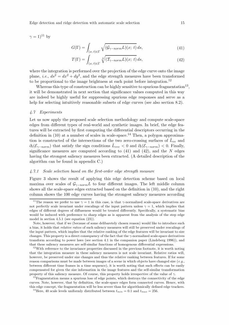
the 50 most significant edges the 20 most significant edges the 10 most significant edges
Figure 4: Illustration of the ranking on saliency obtained from the integrated γ-normalizedgradient magnitude along the scale-space edges. Here, the 50, 20, and 10 most significantscale-space edges, respectively, have been selected from the arm image.
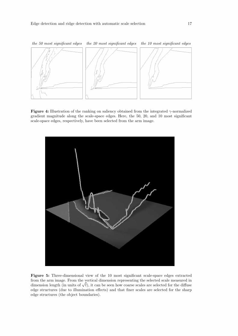
Figure 5: Three-dimensional view of the 10 most significant scale-space edges extractedfrom the arm image. From the vertical dimension representing the selected scale measured indimension length (in units of
√t), it can be seen how coarse scales are selected for the diffuse
edge structures (due to illumination effects) and that finer scales are selected for the sharpedge structures (the object boundaries).

18 Lindeberg
original image the 100 strongest edge curves the 10 strongest edge curves
Figure 6: Corresponding results of applying the edge detection method with automatic scaleselection to an image of a detail of a table (containing strong effects of focus blur). Here, the100 and the 10 strongest edge responses, respectively, have been extracted.
Figure 7: Three-dimensional view of the three strongest scale-space edges extracted fromthe image in figure 6 (showing a detail of a table registered with a narrow depth of field).Observe how the selected scale levels (graphically represented by the height of the curves overthe image plane) reflect the variation in the amount of focus blur along the edge.

Edge detection and ridge detection with automatic scale selection 19
original grey-level image all scale-space edges the 100 strongest edge curves
Figure 8: The result of edge detection with automatic scale selection based on local maximaover scales of Tγ−normL (with γ = 1
2). The middle column shows all the scale-space edges,
whereas the right column shows the 100 edge curves having the highest significance values(according to (42)). Image size: 256×256 pixels for the two top-most images, 143×143 pixelsfor the statue image, and 182 × 182 pixels for the fractal image.

20 Lindeberg
original grey-level image the 1000 most salient scale-space edges
Figure 9: The result of edge detection with automatic scale selection using local maximaover scales of Tγ−normL (with γ = 1
2) for two images containing a large number of fine-scale
details. Observe how well the fine-scale structures are captured and resolved. (Image size:256 × 256 pixels for the Godthem Inn image and 240× 240 for the Paolina image.)

Edge detection and ridge detection with automatic scale selection 21
to (41). As can be seen, a large number of edges is obtained, corresponding to objectboundaries, shadow edges, as well as spurious structures in the smooth background.
For the arm image in the first row, we can observe that the sharp edges corre-sponding to the object boundaries are extracted, as well as the shadow edges on thearm, the cast shadow on the table, and the reflection on the table. In other words, thescale selection procedure leads to a qualitatively very reasonable extraction of edgeswith the scale levels adapted to the local image structure. (Recall from figure 2 thatfor this image it is impossible to capture the entire shadow edge at one scale withoutintroducing severe shape distortions at the finger tip.)
The second and the third rows show corresponding results for an indoor officescene and an outdoor image of a statue. As can be seen, the major edges of theobjects are extracted, as well as the occlusion shadow on the cylindrical object in theright part of the image. For the outdoor image, the outline of the statue is extracted,some parts of the shadows on the ground, the outline of the forest at the horizon, aswell as an outline of the clouds in the sky.
The fourth row shows the result of applying the edge detection procedure to a frac-tal image. This example is interesting, since the image contains structures of differenttypes and at a large number of different scales. As can be seen, the edge detectorcaptures a large number of different features, and among the 100 strongest edges wefind the boundaries of the bright blob structures and a subset of the boundary edgeshaving highest contrast.
Of course, the number of edges selected for display is arbitrary, and in an inte-grated vision system, some mechanism is required for evaluating how many of theedges correspond to meaningful image structures in a given situation. We argue,however, that the significance values provide important information for making suchdecisions. Figure 4 illustrates this property, by showing the 50, 10 and 5 strongestedges, respectively, extracted from the arm image. As can be seen, the outlines of thearm, the table and the cast shadow are among the most significant edges.
Figure 5 gives a three-dimensional illustration of how the selected scale levelsvary along the edges. In this figure, the 10 most salient scale-space edges have beenextracted from the arm image and visualized as one-dimensional curves embeddedin the three-dimensional scale-space representation. These curves in scale-space havebeen overlayed on top of a low-contrast copy of the original grey-level image, andare seen from an oblique view with the height over the image plane representing theselected scale measured in dimension length (in units of
√t). From this illustration,
it can be seen how fine scales have been selected at the object boundaries, and thatcoarser scales are selected with increasing degree of diffuseness.
Figure 6 shows another illustration of how diffuseness estimates are obtained fromthis edge detector. It shows edges detected from an image of a detail of table, forwhich the effects of focus blur are strong. Note how the selected scale levels capturethe varying degree of diffuseness along the edges (see figure 7).
4.7.2 Scale selection based on the third-order edge strength measure
Figure 8 shows corresponding results of edge detection with scale selection basedon local maxima over scales of Tγ−normL. To a first approximation, the results arequalitatively similar. At the more detailed level, however, we can observe that theperformance is slightly better in the respect that more responses are obtained for theshadow edges in the indoor office image and for the outdoor statue image. An intuitiveexplanation of why the edge strength measures differ in this respect, is that the third-

22 Lindeberg
order derivative operator has more narrow response properties to edges. Therefore, themagnitude of this response will start to decrease earlier with scale, when interferenceeffects between neighbouring edges start affecting the edge responses.
Figure 9 shows the performance of this scale selection method when applied totwo images containing a large amount of fine-scale structures. From a first view,these results may look very similar to the result of traditional edge detection at afixed (very fine) scale. A more detailed study, however, reveals that a number ofshadow edges are extracted, which would be impossible to detect at the same scaleas the dominant fine-scale information. In this context, it should be noted that thisdetection of edges at very fine scales in this case is not the result of any manual settingof tuning parameters. It is a direct consequence of the definition of the scale-spaceedge concept, and is the result of applying the same mechanism as selects coarse scalelevels for diffuse image structures.
4.8 Summary
To conclude,15 for both these measures of edge strength, the proposed scale selectionscheme has the desirable property of adapting the scale levels to the local imagestructure such that the selected scales reflect the degree of diffuseness of the edge.
5 Ridge detection with automatic scale selection
In most current feature based computer vision algorithms, edges are used as the maintype of image features. This historical heritage should, however, not exclude the use ofother features. For example, blob descriptors can deliver important hypotheses aboutthe existence of objects, signalling that ”there might be something there of about thatsize—now some other processing module could take a closer look” (Lindeberg 1993a).A ridge feature can be seen as a refined version of such a descriptor, which in addi-tion provides an approximate symmetry axis of the candidate object. Psychophysicalsupport for this idea have been presented by (Burbeck and Pizer 1995).
When to define ridges from intensity data, there are several possible approaches. Intopography, a ridge is defined as a separator between regions from which water flows indifferent directions (to different sinks). The precise mathematical formulation of thisproperty has, however, lead to a large number of confusions. A historic account of thisdevelopment is given by (Koenderink and van Doorn 1994). In computer vision, earlyapproaches to ridge detection were proposed by (Haralick 1983), who defined bright(dark) ridges as points for which the main principal curvature assumes a maximum(minimum) in the main principal curvature direction, and by (Crowley and Parker1984), who considered directional maxima in bandpass filtered images.
During more recent years, the ridge detection problem has been intensively studiedby Pizer and his co-workers (Pizer et al. 1994). (Gauch and Pizer 1993) define ridgesfrom topographical watersheds computed in a scale-space representation of the imagedata. (Morse et al. 1994) compute ”core” descriptors in a multi-scale fashion bypropagating a measure of edge strength from each edge point and then detecting peaksin the measure of ”medialness” so obtained. A more extensive discussion of differenttypes of ridge detectors is presented by (Eberly et al. 1994), including extensions tohigher dimensions. Related applications of similar ideas to medical images have beenpresented by (Griffin et al. 1992; Monga et al. 1994; Koller et al. 1995).
15A more extensive summary and discussion is given in section 7.1.

Edge detection and ridge detection with automatic scale selection 23
For binary data, the related notion of “skeletons” can be derived from the medialaxis (Blum and Nagel 1978) and be computed by (grass-fire-like) distance transforms(Arcelli and Baja 1992). It is, however, well-known that features extracted in thisway can be highly sensitive to small perturbations of the boundary. To reduce theseproblems, (Ogniewicz and Kubler 1995) proposed a hierarchical skeleton concept. Al-ternatively, this sensitivity can be reduced by grey-level based multi-scale techniques.
In this section, we shall show how the framework for edge detection developed inprevious section, with just minor modifications, can be used for formulating a ridgedetector with automatic scale selection. In analogy with the treatment in section 4, weshall first express a differential geometric ridge detector in terms of local directionalderivatives at a fixed scale in scale-space. Then, we turn to the problem of includinga mechanism for automatic scale selection.
5.1 Local directional derivatives
At any image point (x0, y0), introduce a local (p, q)-system aligned to the principalcurvature directions of the brightness function. To express directional derivatives inthese coordinates, which are characterized by the mixed second-order derivative beingzero, Lpq = 0, we can rotate the coordinate system by an angle β defined by
cos β|(x0,y0)=
√
√
√
√
√
1
2
1 +Lxx − Lyy
√
(Lxx − Lyy)2 + 4L2xy
∣
∣
∣
∣
∣
∣
∣
(x0,y0)
,
(43)
sinβ|(x0,y0)= (sign Lxy)
√
√
√
√
√
1
2
1 − Lxx − Lyy√
(Lxx − Lyy)2 + 4L2xy
∣
∣
∣
∣
∣
∣
∣
(x0,y0)
, (44)
and define unit vectors in the p- and q-directions by ep = (sin β,− cos β) and eq =(cos β, sin β) with associated directional derivative operators
∂p = sin β ∂x − cos β ∂y, ∂q = cos β ∂x + sin β ∂y. (45)
Then, it is straightforward to verify that this definition implies that
Lpq = ∂p∂qL = (cos β ∂x + sin β ∂y) (sin β ∂x − cos β ∂y)L
= cos β sin β (Lxx − Lyy) − (cos2 β − sin2 β)Lxy = 0.(46)
5.2 Differential geometric ridge definition
As mentioned in the introduction to this section, there are several ways to defineridges from intensity data. A natural way to formulate a ridge concept in terms oflocal differential geometric properties of image brightness is by defining a bright (dark)ridge as a connected set of points for which the intensity assumes a local maximum(minimum) in the direction of the main principal curvature. When expressed in the(p, q)-system, this requirement for point to be a bright ridge point can be written
Lp = 0,Lpp < 0,
|Lpp| ≥ |Lqq|,or
Lq = 0,Lqq < 0,
|Lqq| ≥ |Lpp|,(47)

24 Lindeberg
scale-space representation bright ridges scale-space representation bright ridges
t = 1.0
t = 4.0
t = 16.0
t = 64.0
t = 256.0
Figure 10: Ridges computed at different scales for an aerial image and an image of a hand(using the ridge definition in (48)). Notably, different types of image structures give riseto different ridges curves at different scales. In particular, no single scale is appropriate forcapturing all major ridges. (Image size: 128 ∗ 128 and 140 ∗ 140 pixels.)

Edge detection and ridge detection with automatic scale selection 25
depending on whether the p- or the q-direction corresponds to the maximum absolutevalue of the principal curvature. This idea, which goes back to (Saint-Venant 1852),is closely related to the approaches in (Haralick 1983; Eberly et al. 1994).16
In (Lindeberg 1994b) it is shown that in terms of the (u, v)-system described insection 4.1, this condition can for non-degenerate L equivalently be written
{
Luv = 0,L2
uu − L2vv > 0,
(48)
where the sign of Luu determines the polarity; Luu < 0 corresponds to bright ridges,and Luu > 0 to dark ridges.
5.3 The need for automatic scale selection in ridge detection
Figure 10 shows the result of computing ridges defined in this way at different scalesin scale-space for an aerial image of a suburb and an image of an arm, respectively.Observe how different types of ridge structures give rise to ridge curves at differentscales. For example, the main roads in the aerial image appear at t ≈ 64, the fingersgive rise to ridge curves at t ≈ 16, and the arm as a whole is extracted as a long ridgecurve at t ≈ 256. Moreover, note that these ridge descriptors are much more sensitiveto the choice of the scale levels than the edge features in figure 2. In particular,no single scale is appropriate for extracting ridges over the entire image. Hence, amechanism for automatic scale selection is necessary in order to compute these ridgedescriptors from image data about which no a priori information is available.
5.4 Scale selection: Selection of ridge curves on the ridge surface
If the ridge definition (47) is applied at all scales in scale-space, it will sweep out a sur-face in scale-space. This surface will be referred to as the ridge surface in scale-space.To formulate a scale selection method for ridge detection, let us assume that we canassociate a normalized measure of ridge strength RnormL to each point in scale-space.Then, in analogy with section 4.3, we can define a scale-space ridge as the intersectionof the ridge surface with the surface defined by RnormL being locally maximal overscales. Assume, for simplicity, that we in some region can locally rename17 the p-and q-directions such that the p-direction corresponds to the maximum value of theprincipal curvature at each point. Then, a scale-space ridge is defined as a connectedset of points Γ = {(x, y; t) ∈ R
2 × R+} that satisfies
{
∂t(RnormL(x, y; t)) = 0,∂tt(RnormL(x, y; t)) < 0,
{
Lp(x, y; t) = 0,Lpp(x, y; t) < 0.
(49)
Alternatively, we can consider directional derivatives of RnormL computed in thetangent plane of the ridge surface, in analogy with the definition in equation (13).
16 In terms of details, however, the approach by (Eberly et al. 1994) differs from the approachtaken here (and in (Lindeberg 1994b)) in the sense that (Eberly et al. 1994) compute derivatives inthe p- and q-directions by differentiating along the curved trajectories of the (p, q)-system, whereaswe here compute directional derivatives in the tangential directions of this curvi-linear coordinatesystem. For curved ridges, these two approaches will, in general, have different properties.
17Globally, however, we cannot expect to be able to reorient the coordinate system in this way.Hence, when implementing this ridge detection scheme in practice, the logical ”or” operation occur-ring in (47) is always necessary. The simplifying assumption is introduced here with the only purposeof simplifying the presentation and shortening the algebraic expressions.
26 Lindeberg
What remains to turn this definition into an operational method for detectingridges, is to define the measure of ridge strength. In the following sections, we willconsider the consequences of using three such strength measures.
5.5 Measures of ridge strength
Given the ridge definition in (47), the presumably first choice to consider as measureof ridge strength is the maximum absolute value of the principal curvatures
ML = max(|Lpp|, |Lqq|). (50)
If we again introduce normalized derivatives parameterized by a parameter γ suchthat ∂ξ = tγ/2∂x, we obtain the γ-normalized maximum absolute principal curvature
Mγ−normL = max(|Lpp,γ−norm|, |Lqq,γ−norm|) = tγ max(|Lpp|, |Lqq|), (51)
where the explicit expressions for Lpp,γ−norm and Lqq,γ−norm are
Lpp,γ−norm =tγ
2
(
Lxx + Lyy −√
(Lxx − Lyy)2 + 4L2xy
)
, (52)
Lqq,γ−norm =tγ
2
(
Lxx + Lyy +√
(Lxx − Lyy)2 + 4L2xy
)
. (53)
A negative property of this entity, however, is that it is not specific to ridge-like struc-tures, and gives strong responses to other image structures, such as blobs. (Consider,for example, the behaviour when Lxx = Lyy and Lxy = 0.) For this reason, we shallalso consider the following differential expression, which originates from the alterna-tive formulation of the ridge definition in (48). This ridge strength measure will bereferred to as the square of the γ-normalized square principal curvature difference
Nγ−normL = (L2pp,γ−norm − L2
qq,γ−norm)2. (54)
In contrast to Mγ−normL, this entity assumes large values only when the principalcurvatures are significantly different, i.e., for elongated structures. Moreover, there isno logical “or” operation in its differential expression in terms of spatial derivatives
Nγ−normL = ((Lpp,γ−norm + Lqq,γ−norm) (Lpp,γ−norm − Lqq,γ−norm))2
= t4γ (Lxx + Lyy)2 ((Lxx − Lyy)
2 + 4L2xy). (55)
If we want to have a ridge strength measure that completely suppresses the influenceof the Laplacian blob response (∇2L)2 = (Lxx + Lyy)
2, a natural third alternative toconsider is the square of the γ-normalized principal curvature difference.
Aγ−normL = (Lpp,γ−norm − Lqq,γ−norm)2 = t2γ ((Lxx − Lyy)2 + 4L2
xy).(56)
In appendix B, explicit expressions are derived for the first- and second-order deriva-tives of these ridge strength measures with respect to the scale parameter.
5.6 Qualitative properties of different ridge strength measures
Concerning the qualitative behaviour of ridge detectors based on these ridge strengthmeasures, we can first make the general observation that the behaviour is the samefor cylindric image patterns, i.e., image patterns of the form f(x, y) = h(ax + by + c)for some h : R → R and some constants a, b, c ∈ R.18 For image structures withoutsuch symmetry, however, the qualitative behaviour may be different.
18For such image patterns, one of the principal curvatures is zero, and the ridge strength measuresare all proportional to the other principal curvature raised to some power.

Edge detection and ridge detection with automatic scale selection 27
scale-space representation M2γ−normL
√
Nγ−normL Aγ−normL
t = 1.0
t = 4.0
t = 16.0
t = 64.0
t = 256.0
Figure 11: Ridge strength measures computed different scales for an aerial image of a suburb.Notably, different types of ridge structures give rise to strong responses at different scales.Moreover, there are qualitative differences in the response properties of the ridge descriptorsto curved ridges and ridges of finite extent. The ridge strength measures also differ in termsof the extent to which they give spurious responses to blob-like and edge-like structures.

28 Lindeberg
scale-space representation M2γ−normL
√
Nγ−normL Aγ−normL
t = 1.0
t = 4.0
t = 16.0
t = 64.0
t = 256.0
Figure 12: Ridge strength measures computed different scales for an image of a hand. Notethat the fingers and the arm give rise to strong ridge strength responses at the same scales(t ≈ 16 and t ≈ 256) as the fixed-scale ridge detector in figure 10 succeeds in extracting cor-responding ridge curves. Moreover, observe that Nγ−normL has more ridge-specific responseproperties than Mγ−normL and Aγ−normL.

Edge detection and ridge detection with automatic scale selection 29
5.6.1 Cylindrical Gaussian ridge
To study the behaviour for a cylindric ridge in more detail, consider a one-dimensionalGaussian blob with variance t0, extended cylindrically in the perpendicular direction
f(x, y) = g(x; t0), (57)
where g here denotes the one-dimensional Gaussian kernel
g(x; t) =1√2πt
e−x2/(2t). (58)
From the semi-group property of Gaussian smoothing, it follows that the scale-spacerepresentation of f is given by
L(x, y; t) = g(x; t0 + t). (59)
Here, the ridge coincides with the y-axis, and on this ridge we have
(Mγ−normL)(0, y; t) = tγ |gxx(0, y; t)| =1√2π
tγ
(t0 + t)3/2. (60)
Differentiation with respect to t gives
∂t(Mγ−normL)(0, y; t) =1
2√
2π
tγ−1 (2 γ (t + t0) − 3 t)
(t0 + t)5/2, (61)
and setting this derivative to zero
∂t(Mγ−normL)(0, y; t) = 0 ⇔ tMγ−norm=
2 γ
3 − 2 γt0. (62)
Clearly, 0 < γ < 32 is a necessary condition to give a local maximum over scales.
Moreover, γ = 1 corresponds to tMγ−norm= 2 t0. If we want the selected scale level to
reflect the width of the ridge such that tMγ−norm= t0, then we should select γ = 3
4 .
5.6.2 Simulation experiments
Because of the complexity of the differential expressions for these ridge strengthmeasures, it is hard to find representative ridge models that allow for compact closed-form analysis of curved ridges. For this reason, let us instead illustrate the qualitativebehaviour by simulations on real-world data.
Figures 11–12 show the result of computing the three ridge strength measures,Mγ−normL, Nγ−normL and Aγ−normL, at different scales for an aerial image of asuburb and an image of a hand, respectively. For all these descriptors different types ofimage structures give rise to different types of responses at different scales. Specifically,strong responses are obtained when the standard deviation of the Gaussian kernel isapproximately equal to the width of the ridge structure. (Observe that the fixed-scaleridge detector in figure 10 extracts nice ridge curves at these scales.)
It can also be seen that the ridge descriptors have qualitative different behavioursin the way they respond to curved ridge structures, ridges of finite length, and tothe extent they generate spurious responses at blob structures and edge structures.Notably, Mγ−normL and Aγ−normL give strong responses at edges, and Mγ−normLalso comparably strong blob responses. In this respect, Nγ−normL appears to havethe most ridge-specific response properties of these descriptors.
30 Lindeberg
5.7 Experiments
Let us now show the result of applying integrated ridge detectors with automaticscale selection to different types of real-world images.
In analogy with section 4.7, we first compute the differential descriptors occurringin the definition of a scale-space ridge (49) at a number of scales in scale-space19
Then, polygons are constructed to approximate the intersections of the two zero-crossing surfaces of Lp and ∂t(Rγ−norm) that satisfy the sign conditions Lpp < 020
and ∂t(Rγ−norm) < 0. Finally, a significance measure is is computed for each ridgecurve in a way analogous to section 4.6.1.
5.7.1 Measures of ridge saliency
To have the significance measures proportional to the local brightness contrast, thestrength measures are again transformed before integration. For any scale-space ridgeΓ, and for each measure of ridge strength, the saliency measure is defined by:
M(Γ) =
∫
(x; t)∈Γ(Mγ−norm)(x; t) ds, (63)
N(Γ) =
∫
(x; t)∈Γ
4
√
(Nγ−norm)(x; t) ds, (64)
A(Γ) =
∫
(x; t)∈Γ
√
(Aγ−norm)(x; t) ds, (65)
where the integration is again performed by projecting the scale-space ridge onto theimage plane ds2 = dx2 + dy2.
5.7.2 Scale selection based on Mγ−norm and Aγ−norm
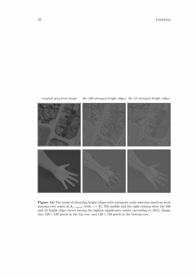
Figure 13 and figure 14 show the result of detecting bright ridges from the aerialimage of the suburb and the image of the arm in figure 10, using scale selection basedon maxima over scales of Mγ−norm and Aγ−norm, respectively. As can be seen, themajor roads are extracted from the aerial image. For the image of the arm, ridgedescriptors are extracted for each one of the fingers. In addition, a coarse-scale ridgeis obtained for the arm as a whole.
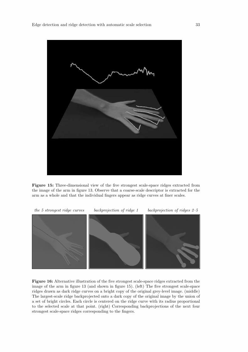
Figure 15 shows a three-dimensional illustration of the result from the arm image.Here, the five most significant scale-space ridges have been drawn as three-dimensionalcurves in scale-space with the height over the image plane representing the selectedscale at each ridge point. Note how the selected scale levels reflect the widths of ridges.
Figure 16 shows another illustration of this data, where each ridge curve has beenrepresented by a region, constructed from the union of circles centered at the pointson the ridge curve, and with the radius proportional to the selected scales measuredin dimension length.
5.8 Summary
To conclude,21 we have shown that for both these measures of ridge strength, theproposed scale selection scheme has the desirable property of adapting the scale levelsto the local image structure such that the selected scales reflect the width of the ridge.
19Here, 40 scale levels uniformly distributed between tmin = 1 and tmax = 512.20This condition concerns bright ridges. For dark ridges, it is, of course, changed to Lpp > 0.21A more extensive summary and discussion is given in section 7.2.

Edge detection and ridge detection with automatic scale selection 31
original grey-level image the 100 strongest bright ridges the 10 strongest bright ridges
Figure 13: The result of detecting bright ridges with automatic scale selection based on localmaxima over scales of Nγ−norm (with γ = 3
4). The middle and the right column show the 100
and 10 bright ridge curves having the highest significance values (according to (65)). Imagesize: 128 × 128 pixels in the top row, and 140× 140 pixels in the bottom row.
32 Lindeberg
original grey-level image the 100 strongest bright ridges the 10 strongest bright ridges
Figure 14: The result of detecting bright ridges with automatic scale selection based on localmaxima over scales of Aγ−norm (with γ = 3
4). The middle and the right column show the 100
and 10 bright ridge curves having the highest significance values (according to (65)). Imagesize: 128 × 128 pixels in the top row, and 140× 140 pixels in the bottom row.
Edge detection and ridge detection with automatic scale selection 33
Figure 15: Three-dimensional view of the five strongest scale-space ridges extracted fromthe image of the arm in figure 13. Observe that a coarse-scale descriptor is extracted for thearm as a whole and that the individual fingers appear as ridge curves at finer scales.
the 5 strongest ridge curves backprojection of ridge 1 backprojection of ridges 2–5
Figure 16: Alternative illustration of the five strongest scale-space ridges extracted from theimage of the arm in figure 13 (and shown in figure 15). (left) The five strongest scale-spaceridges drawn as dark ridge curves on a bright copy of the original grey-level image. (middle)The largest-scale ridge backprojected onto a dark copy of the original image by the union ofa set of bright circles. Each circle is centered on the ridge curve with its radius proportionalto the selected scale at that point. (right) Corresponding backprojections of the next fourstrongest scale-space ridges corresponding to the fingers.
34 Lindeberg
6 Relations to previous works
Because of the range of topics spanned by this article, there are several links toprevious works in addition to those already pointed out in the introductory sections.
The normalized gradient magnitude (with γ = 1) has been used also by (Korn1988), for relating thresholds on gradient magnitude at different scales. Inspired bythe early work by (Marr 1976), who observed that variations of the step size ina finite difference operator gives rise to different types of signatures depending onthe edge type, (Zhang and Bergholm 1993) studied ways of classifying edges basedon the evolution properties over scales of the normalized gradient magnitude. Theirapproach was to first accumulate the signature and then to fit a pre-defined modelto the data. Related techniques have been presented by (Mallat and Zhong 1992),who characterize edges from the Lipschitz exponents of wavelet descriptors, (Lu andJain 1989) who reason about the behaviour of Laplacian zero-crossings in scale-space,and (Rohr 1992) who fit parametric junction and edge models to the image data toestimate the degree of diffuseness.
The notion of scale-space edge proposed here unifies the ideas of such diffusenessestimation schemes with the standard method for edge detection by non-maximumsuppression proposed by (Canny 1986) and (Korn 1988). Moreover, the use of normal-ized derivatives in edge detection (Korn 1988; Zhang and Bergholm 1993), and thegeneral idea of using maxima over scales of normalized derivatives for scale selectionfor feature detectors (Lindeberg 1993c, 1994a), are here furthered to the notion ofscale selection based on γ-normalized derivatives. In addition, a third-order measureof edge strength is introduced, and an integrated edge detection scheme is presentedin terms of the intersection of zero-crossing surfaces in scale-space. The local max-imization of the edge strength measures across scales also provides a way to adaptthe scale levels to the local image structures in such a way that the scale levels mayvary along the edge, and diffuseness estimates be obtained directly when detectingedges and based on local operations only. Compared to the approach by (Zhang andBergholm 1993) there is hence no need for explicitly accumulating the signature bylinking edges across scales, or to fit a model to the data to estimate the degree ofdiffuseness. Corresponding differences hold in relation to the works by (Mallat andZhong 1992; Lu and Jain 1989; Rohr 1992).
The ridge detectors proposed by (Pizer et al. 1994; Eberly et al. 1994; Koller etal. 1995) also involve the maximization of certain strength measures across scales.In this respect, they are closely related to the scale selection principle used in thiswork. The methods in (Pizer et al. 1994; Koller et al. 1995), however, differ in therespect that they are non-local and construct ridges by propagating edge informationfrom corresponding boundaries. The ridge detection scheme in (Eberly et al. 1994) iscloser to this approach in the sense that it is local. This work differs, however, in thedetailed ridge definition (see footnote 16), in the choice of ridge strength measures,and the explicit construction of ridges as intersections of zero-crossing surfaces. Theuse of γ-normalized derivatives instead of ordinary normalized derivatives also allowsfor a more direct control of the scale levels to be selected.22
The strongest connection to other works, however, is that this article makes ex-plicit how the scale selection principle proposed in (Lindeberg 1991, 1993c, 1994a)can be used for constructing integrated algorithms for detecting edges and ridges.
22Note that (as shown in section 5.6.1) the use of ordinary normalized derivatives (with γ = 1)leads to the selection of much coarser scale levels than with this approach (using γ = 3
4).

Edge detection and ridge detection with automatic scale selection 35
7 Summary and discussion
We have presented a framework for automatic scale selection for detecting one-dimensional features, such as edges and ridges, from image data. Compared to atraditional approach of defining and extracting such features from a grey-level imageat a fixed level of scale (or a set of such fixed scales), we have proposed that it ismore natural to define the concepts of edges and ridges as one-dimensional curves inthe three-dimensional scale-space representation of the image (spanned by the spaceand scale dimensions). A basic reason why such a definition is more useful is that ingeneral situations it will hardly ever be the case that a vision system can know inadvance what scales are appropriate for analysing the image structures in a given im-age. Therefore, a mechanism for automatic scale selection is a necessary complementto traditional multi-scale processing in general, and feature detection in particular.
As we have illustrated by examples, a single scale level will usually not be appro-priate for extracting the relevant edges in a real-world image of a scene of moderatecomplexity. For example, at distinct edge structures, such as sharp edges due at ob-ject boundaries with high contrast, the amount of smoothing should usually be assmall as possible, to not affect the localization of the edges more than necessary.Conversely, at more diffuse edges structures, such as edges due to illumination effectsand edge structures subject to out-of-focus blur, a substantial amount of smoothingmay be required before the edge detector is able to produce coherent edge curves.Comparably coarse scales for edge detection will also be necessary if the noise level ishigh, or if other interfering fine-scale structures are present, such as surface texture.To achieve an appropriate trade-off in the well-known conflict between detection andlocalization, we must therefore allow the scale levels for edge detection to vary overthe image. Specifically, to capture edges with varying degree of diffuseness, such ascast shadows, it will be necessary to let the scale levels vary along the edge. Similarproblems arise when extracting ridges from image data. The general conclusion isthat the scale level should be of the same order as the width of the ridge structure,and that a ridge detector is usually much more sensitive to the choice of scale levelsthan an edge detector.
7.1 Edge detection with automatic scale selection
To cope with the scale problem in edge detection, we proposed an extension of thenotion of non-maximum suppression to include the scale dimension already in the edgedefinition. In addition to the usual requirement, that the gradient magnitude shouldassume a maximum in the gradient direction (which gives rise to an edge surface inscale-space), we proposed to define a scale-space edge by simultaneous maximizationof a (normalized) measure of edge strength over scales.
Specifically, we considered the consequences of using two such measures of edgestrength in more detail—the γ-normalized square gradient magnitude, Gγ−norm, andthe negative γ-normalized third-order directional derivative in the gradient direc-tion multiplied by the gradient magnitude raised to the power of three, Tγ−norm.By theoretical analysis for a set of characteristic edge models and by experimentson real-world data, we demonstrated that the qualitative behaviour of the composededge detection method is to select fine scales for sharp edge structures and to se-lect coarse scales when extracting diffuse edges. Hence, the resulting scale selectionmechanism has the desirable property of adapting the scale levels for edge detectionto the local image structure. By such automatic selection of local appropriate scales

36 Lindeberg
for edge detection, we have not only eliminated the need for external choice of scalelevels for the edge detection module. We have also obtained a methodology for edgedetection, which can be expected to be more robust to changes in the environment.Notably, the behaviour of scale selection method is not the result of any rule-basedsystem. Instead, it follows as a direct consequence of the proposed edge definition.
Another important property of this approach is that the edge detector simulta-neously determines an estimate of edge diffuseness as attribute to each edge point.Such information provides useful clues to the physical nature of the edge, which, forexample, can be used for distinguishing object edges from shadow edges, and forestimating relative depth based on focus blur.
7.2 Ridge detection with automatic scale selection
Then, we turned to the problem of ridge detection. It was shown that by minor mod-ifications, similar ideas could be used for formulating a ridge detector with automaticscale selection. A traditional fixed-scale differential geometric ridge definition, whichmeans that bright (dark) ridges at any scale are defined as points for which the mainprincipal curvature assumes a maximum (minimum) in the gradient direction, was ex-tended to the scale dimension, and the concept of a scale-space ridge was introduced,by maximizing a (normalized) measure of ridge strength over scales.
Specifically, three measures of ridge strength were considered in more detail, theγ-normalized main principal curvature, Mγ−norm the γ-normalized square differenceof the square principal curvatures, Nγ−norm, and the γ-normalized square differenceof the principal curvatures, Aγ−norm. For ridges with one-dimensional symmetry, allthese entities have the same scale selection properties, and give rise to scale levelscorresponding to the width of the ridge. Hence, in addition to automatic adaptationof the scale levels for ridge detection to the local image structure, this feature detectorreturns an estimate of the width of the ridge associated with each ridge point. Thisattribute information is important when mapping ridge features to the image regionsthey arose from.
7.3 Scale-space derivatives of high order
The scale selection methodologies presented here are based on the zero-crossings ofdifferential invariants containing derivatives up to order five, and the sign of differen-tial invariants containing derivatives up to order seven. Sometimes it has been arguedthat for practical purposes it is very hard or even impossible to compute derivativesof order two or higher on real-world image data. With the results presented in thiswork, we have on the other hand demonstrated that highly useful results can indeedbe obtained for much higher orders of differentiation, provided that the derivative ap-proximations are computed in a multi-scale framework and combined with an explicitmechanism for scale selection as well as a carefully chosen discrete implementation.
8 Extensions and further work
8.1 Multiple feature responses at different scales
An important property of feature detectors designed according to this framework isthat they will have the ability to respond to different types of image structures atdifferent scales, which is impossible for a fixed-scale edge detector operating at asingle level of scale. A fundamental problem in this context, however, concerns howto combine features extracted at different scales for further processing. For certain
Edge detection and ridge detection with automatic scale selection 37
types of image data, we can expect qualitatively different types of interpretationsto be possible depending on the scale of the analysis. One example is the classicalabstraction hierarchy: forest–tree–branch–leaf. In this work, we have not made anyeffort to address this problem by integrating edge descriptors at different scales. Itis worth pointing out, however, that if this scheme is applied to such image data, itwill respond to the outline of the tree at some coarse scale, and to the outlines of theleaves at some finer scales.23
8.2 Selective mechanisms
Another basic problem concerns the design of selective mechanisms. Whereas thisscale selection methodology produces a much more compact set of edge descriptorsthan a fixed-scale edge detection at a corresponding set of scales, there is a need forranking the edges on saliency to suppress spurious responses and to allow subsets ofthe most salient edges to be selected. One of the most common ways of suppressingspurious edge responses is by (hysteresis) thresholding on the gradient magnitude. Ofcourse, the approach presented here is compatible with such thresholding techniques(preferably based on the normalized measures of feature strength). The inherent limi-tations of such techniques, however, suggest that richer sources of information shouldbe used already in the earliest processing stages. The saliency measures introducedin section 5.5, constitute a step in this direction. More generally, one could conceiveincluding stability properties of the features in scale-space, such as their scale-spacelifetime, based on the explicit registration of bifurcation events (Lindeberg 1993a).
8.3 Alternative approaches to feature detection
Throughout this work we have focused on the detection of edge and ridge featuresrepresented as one-dimensional curves, following the dominant approach to machinevision today, based on sparse image features of low dimension. Extracting curve de-scriptors explicitly, however, leads to a number of technical complications, and withrespect to a number of visual tasks one could conceive using only responses fromdifferential operators (direct computation by dense feature descriptors), or to repre-sent edges and ridges by regions instead of curves. In principle, there is nothing thatprevents the ideas behind this approach from being extended in such ways.24
Concerning the specific implementations of feature detection algorithms presented,they have been based on standard techniques, and the measures of feature strengthchosen because of their intimate connections to the differential geometric feature de-tectors used. Whereas we by these experiments have shown that the resulting method-ology allows highly useful image descriptors to be extracted in a completely automaticway, the design choices made here should be interpreted as excluding the possibilitythat future work may show that other differential descriptors could improve the per-formance further.25 The most important contribution of this work in this respect isthat it opens up a general framework for scale selection, in which further develop-ments and refinement of early visual modules can be performed, by integrating them
23Provided that there is a brightness contrast relative to the background and the resolution issufficiently high for the leaves to be resolved.
24Compare, for example, with the dense pseudo-quadrature responses in (Lindeberg 1994a), andthe multi-scale blob extraction in (Lindeberg 1993a).
25For example, an interesting path to follow is to investigate if more explicit local estimates of signalto noise ratios can be included in the measures of feature strength, analogously to the minimizationof error measures in the second localization step in (Lindeberg 1994a).

38 Lindeberg
with explicit mechanisms for scale selection.
9 Conclusion: Principles for scale selection
To conclude, this work combined with the earlier work in (Lindeberg 1993c, 1994a)shows that detection of local maxima over scales of normalized differential entities pro-vides a consistent framework for generating hypothesis about local appropriate scalesfor detecting image features such as blobs, corners, edges and ridges.
A related methodology for scale selection, for computing local image deformationssuch as optic flow and when performing image matching, is presented in (Lindeberg1995). There, hypotheses about appropriate scales are generated from the scale levelsat which normalized error measures assume local minima over scales.
These general principles, implying that in the absence of further evidence, scalelevels are selected from the scales at which the normalized response is as strongest,or the scale levels at which the error in the computed estimates are as smallest, maybe far more general than the actual implementations presented so far.
Acknowledgments
This work was partially performed under the ESPRIT-BRA project InSight and theESPRIT-NSF collaboration Diffusion. The support from the Swedish Research Coun-cil for Engineering Sciences, TFR, is gratefully acknowledged.
The three-dimensional illustrations in figure 5, 7 and 15 have been produced withthe kind assistance of Pascal Grostabussiat.
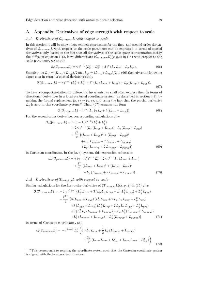
Edge detection and ridge detection with automatic scale selection 39
A Appendix: Derivatives of edge strength with respect to scale
A.1 Derivatives of Gγ−normL with respect to scale
In this section it will be shown how explicit expressions for the first- and second-order deriva-tives of Gγ−normL with respect to the scale parameter can be expressed in terms of spatialderivatives only, based on the fact that all derivatives of the scale-space representation satisfythe diffusion equation (16). If we differentiate (Gγ−normL)(x, y, t) in (14) with respect to thescale parameter, we obtain
∂t(Gγ−normL) = γ tγ−1 (L2x + L2
y) + 2 tγ (Lx Lxt + Ly Lyt). (66)
Substituting Lxt = (Lxxx+Lxyy)/2 and Lyt = (Lxxy+Lyyy)/2 in (66) then gives the followingexpression in terms of spatial derivatives only
∂t(Gγ−normL) = γ tγ−1 (L2x + L2
y) + tγ (Lx (Lxxx + Lxyy) + Ly (Lxxy + Lyyy)).(67)
To have a compact notation for differential invariants, we shall often express them in terms ofdirectional derivatives in a local preferred coordinate system (as described in section 4.1), bymaking the formal replacement (x, y) 7→ (u, v), and using the fact that the partial derivativeLu is zero in this coordinate system.26 Then, (67) assumes the form
∂t(Gγ−normL) = tγ−1 Lv (γ Lv + t (Luuv + Lvvv)). (68)
For the second-order derivative, corresponding calculations give
∂tt(Gγ−normL) = γ (γ − 1) tγ−2 (L2x + L2
y)
+ 2 γ tγ−1 (Lx (Lxyy + Lxxx) + Ly (Lxxy + Lyyy)
+tγ
2
(
(Lxxx + Lxyy)2 + (Lxxy + Lyyy)
2
+Lx (Lxxxxx + 2 Lxxxyy + Lxyyyy)
+Ly (Lxxxxy + 2 Lxxyyy + Lyyyyy)) (69)
in Cartesian coordinates. In the (u, v)-system, this expression reduces to
∂tt(Gγ−normL) = γ (γ − 1) tγ−2 L2v + 2 γ tγ−1 Lv (Luuv + Lvvv)
+tγ
2
(
(Luuu + Luvv)2 + (Luuv + Lvvv)2
+Lv (Luuuuv + 2 Luuvvv + Lvvvvv)) . (70)
A.2 Derivatives of Tγ−normL with respect to scale
Similar calculations for the first-order derivative of (Tγ−normL)(x, y; t) in (15) give
∂t(Tγ−normL) = − 3 γ t3 γ−1 (L3x Lxxx + 3 (L2
x Ly Lxxy + Lx L2y Lxyy) + L3
y Lyyy)
− t3 γ
2
(
3 (Lxxx + Lxyy) (L2x Lxxx + 2 Ly Lx Lxxy + L2
y Lxyy)
+3 (Lyyy + Lxxy) (L2x Lxxy + 2 Ly Lx Lxyy + L2
y Lyyy)
+3 (L2x Ly (Lxxxxy + Lxxyyy) + Lx L2
y (Lxxxyy + Lxyyyy))
+L3x (Lxxxxx + Lxxxyy) + L3
y (Lxxyyy + Lyyyyy))
(71)
in terms of Cartesian coordinates, and
∂t(Tγ−normL) = − t3 γ−1 L2v
(
6 γ Lv Lvvv +t
2Lv (Luuvvv + Lvvvvv)
+3 t
2(Luuu Luvv + L2
uvv + Luuv Lvvv + L2vvv)
)
(72)
26This corresponds to rotating the coordinate system such that the Cartesian coordinate systemis aligned with the local gradient direction.

40 Lindeberg
in the local (u, v)-system The Cartesian expression for the second-order derivative muchlarger.27 When expressed in terms of the local (u, v)-system, it reduces to
∂tt(Tγ−normL) = − 3 γ (3 γ − 1) t3 γ−2 L3v Lvvv
− 3 γ t3 γ−1 L2v
(
Lv (Lvvvvv + Luuvvv)
+3 (L2vvv + L2
uvv + Lvvv Luuv + Luvv Luuu))
− t3 γ
4
(
12 Lv Luvv (Lvvv + Luuv) (Luvv + Luuu)
+6(
Lv
(
Lvvv (Lvvv + Luuv)2 + Luuv (Luvv + Luuu)2)
+L2v ((Lvvv + Luuv) (Lvvvvv + Luuvvv)
+(Luvv + Luuu) (Luvvvv + Luuuvv)))
+L3v (Lvvvvvvv + 2 Luuvvvvv + Luuuuvvv)
+3 L2v
(
Lvvv (Lvvvvv + 2 Luuvvv + Luuuuv)
+Luvv (Luvvvv + 2 Luuuvv + Luuuuu))
)
. (73)
B Appendix: Derivatives of ridge strength with respect to scale
In this appendix, explicit expressions are derived for the first- and second-order scale deriva-tives of the ridge strength measures defined in section 5.5.
Let us again follow the methodology in section 4.4 and appendix A.1, and use the diffusionequation for replacing derivatives of L with respect to t by to derivatives of L with respectto x and y. Applying this procedure to the first- and second-order derivatives of Lpp,γ−norm
with respect to the scale parameter gives:28
∂t(Lpp,γ−norm) = γ tγ−1
(
Lxx + Lyy −√
(Lxx − Lyy)2 + 4 L2xy
)
+tγ
2
Lxxxx + 2 Lxxyy + Lyyyy
− (Lxx − Lyy) (Lxxxx − Lyyyy) + 4 Lxy (Lxxxy + Lxyyy)√
(Lxx − Lyy)2 + 4 L2xy
.
∂tt(Lpp,γ−norm) = γ (γ − 1) tγ−2
(
Lxx + Lyy −√
(Lxx − Lyy)2 + 4 L2xy
)
+tγ
4S1
+ γ tγ−1
(
Lxxxx + 2 Lxxyy + Lyyyy
− (Lxx − Lyy) (Lxxxx − Lyyyy) + 4 Lxy (Lxxxy + Lxyyy)√
(Lxx − Lyy)2 + 4 L2xy
27In unfactorized form, the polynomial expression contains 251 partial derivatives of L.28∂tα(Lqq,γ−norm) can be obtained from these expressions by changing the sign of each square root.

Edge detection and ridge detection with automatic scale selection 41
where
S1 = Lxxxxxx + 3 (Lxxxxyy + Lxxyyyy) + Lyyyyyy
+(4 Lxy (Lxxxy + Lxyyy) + (Lxx − Lyy) (Lxxxx − Lyyyy))
2
(
(Lxx − Lyy)2 + 4 L2xy
)3/2
+(Lxxxx − Lyyyy)
2 + (Lxx − Lyy) (Lxxxxxx + LxxxxyyLxxyyyy − Lyyyyyy)√
(Lxx − Lyy)2 + 4 L2xy
− 4 ((Lxxxy + Lxyyy)2 + Lxy (Lxxxxxy + 2 Lxxxyyy + Lxyyyyy))√
(Lxx − Lyy)2 + 4 L2xy
These expressions simplify somewhat if we rewrite them in terms of local directional deriva-tives in the (p, q)-system. If we, in addition, apply the simplifying assumption Lpp > Lqq,which suppresses all occurrences of sign(Lpp −Lqq), then ∂t(Lpp,γ−norm) and ∂tt(Lpp,γ−norm)reduce to the form
∂t(Lpp,γ−norm) = 2 γ tγ−1 Lpp + tγ (Lpppp + Lppqq) (74)
∂tt(Lpp,γ−norm) = 2 γ (γ − 1) tγ−2 Lpp
+ 2 γ tγ−1 (Lpppp + Lppqq)
+tγ
2
(
Lppppqq + 2 Lppqqqq + Lqqqqqq
− (Lpppp + Lqqqq)2 + 2 (Lpppq + Lpqqq)
2
Lpp − Lqq
)
(75)
For the first-order derivatives of Nγ−normL, corresponding calculations followed by simplifi-cations to the (p, q)-system give
∂t(Nγ−normL) = 2 t4 γ (L2pp − L2
qq) (Lpp (Lpppp + Lppqq) − Lqq (Lppqq + Lqqqq))
∂tt(Nγ−normL) = 2 t4 γ (L2pp − L2
qq) (Lpppp − Lqqqq) (Lqqqq + 2 Lppqq + Lpppp) +t4 γ
2S2
where
S2 = (Lpp − Lqq)2
(
(Lqqqq + 2 Lppqq + Lpppp)2
+(Lpp + Lqq) (Lqqqqqq + 3 (Lppqqqq + Lppppqq) + Lpppppp))
+ (Lpp + Lqq)2
(
4 (Lpppq + Lpqqq)2 + (Lpppp − Lqqqq)
2
+(Lpp − Lqq) (−Lqqqqqq − Lppqqqq + Lppppqq + Lpppppp))
Finally, for Aγ−normL, the first- and second-order scale derivatives are
∂t(Aγ−normL) = t2 γ−1 (Lpp + Lqq) (2 γ (Lpp − Lqq) + t (Lpppp − Lqqqq)) , (76)
∂tt(Aγ−normL) = 2 γ (2 γ − 1) t2 γ−2 (Lpp + Lqq)2
+ 4 γ t2 γ−1 (Lpp + Lqq) (Lpppp − Lqqqq)
+t2 γ
2
(
(Lpppp − Lqqqq)2 + 4 (Lpqqq + Lpppq)
2
+(Lpp + Lqq) (Lpppppp + Lppppqq − Lppqqqq − Lqqqqqq)) .(77)

42 Lindeberg
C Appendix: Detailed algorithmic description
According to the definitions in section 4.3 and 5.4, scale-space edges and scale-space ridgesrespectively are is defined as the intersections of the zero-crossing surfaces of two differentialinvariants Z1L and Z2L that satisfy the sign conditions S1L < 0 and S2L < 0 for two otherdifferential descriptors S1L and S2L.
To compute these features from image data, we have made a rather straightforward ex-tension of the single-scale edge detection method developed in (Lindeberg 1993b), based onthe following types of visual front-end operations:
• smoothing by (large support) convolution with a discrete Gaussian kernel,
• discrete derivative approximations from (small support) finite differences,
• (pointwise) combination of these descriptors to differential invariants, and
• interpolation for zero-crossings (by nearest neighbour comparisons).
In summary, the composed algorithms for multi-scale edge and ridge detection consist of thefollowing major processing steps:
C.1 Pre-processing: Computation of differential invariants
In an initial processing step, differential geometric descriptors are computed based on thescale-space framework for discrete signals described in (Lindeberg 1994c):
• Choice of scale range: Given a discrete image f of a certain size, select a scale range forthe analysis.29 Within this interval, distribute a set of scale levels30 tk, such that theratio between successive scale values tk+1/tk is approximately constant. A natural wayto distribute these scales, is such that the difference in effective scale between adjacentscales τk+1 − τk is approximately constant.
• Scale-space smoothing:. For each scale tk, compute the scale-space representation of fby separable convolution with the discrete analogue of the Gaussian kernel T : L(·; tk) =T (·; tk) ∗ f . (Alternatively, use the non-separable discrete analogue, which allows forhigher degree of rotational invariance.)
• Discrete approximation of γ-normalized differential invariants: For each point at eachscale, compute discrete derivative approximations of L(·; tk) by central differences,combine these into discrete approximations of the differential invariants, and multiplythe result by appropriate powers of tk. Alternatively, normalize the discrete derivativeapproximation kernels to be constant over scales in appropriately selected lp-norms,based on the constant Lp-norm interpretation of the γ-normalized derivative conceptdescribed in the companion paper (Lindeberg 1994a).
C.2 Tracking the intersection of the zero-crossing surfaces
Given access to the differential invariants defining the zero-crossing surfaces, the next step isto construct a polygon approximation of the intersection of these surfaces.
In this implementation, we traverse all voxels in a way closely related to the marchingcubes (Lorensen and Cline 1987) and the marching lines (Thirion and Gourdon 1993) algo-rithms. For each voxel, a test is made if there the intersection of iso-surfaces passes throughthat voxel. Then, on top of this construction, a tracking algorithm operates and links linesegments into polygons, by following the end points of each detected line segment to the nextvoxel. In this way, connected polygons are obtained without any need for further combinatorialprocessing. At an overview level, this surface intersection algorithm works as follows:
29Here, for images of size up to 256 × 256 pixels, we have used tmin = 0.1 and tmax = 256 whendetecting edges and tmin = 1 and tmax = 512 when detecting ridges. (These scale ranges can, ofcourse, be narrowed if further a priori information is available.)
30In this implementation, we have used 40 scales.
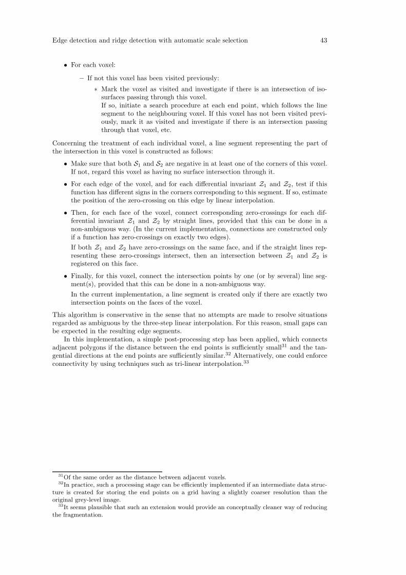
Edge detection and ridge detection with automatic scale selection 43
• For each voxel:
– If not this voxel has been visited previously:
∗ Mark the voxel as visited and investigate if there is an intersection of iso-surfaces passing through this voxel.If so, initiate a search procedure at each end point, which follows the linesegment to the neighbouring voxel. If this voxel has not been visited previ-ously, mark it as visited and investigate if there is an intersection passingthrough that voxel, etc.
Concerning the treatment of each individual voxel, a line segment representing the part ofthe intersection in this voxel is constructed as follows:
• Make sure that both S1 and S2 are negative in at least one of the corners of this voxel.If not, regard this voxel as having no surface intersection through it.
• For each edge of the voxel, and for each differential invariant Z1 and Z2, test if thisfunction has different signs in the corners corresponding to this segment. If so, estimatethe position of the zero-crossing on this edge by linear interpolation.
• Then, for each face of the voxel, connect corresponding zero-crossings for each dif-ferential invariant Z1 and Z2 by straight lines, provided that this can be done in anon-ambiguous way. (In the current implementation, connections are constructed onlyif a function has zero-crossings on exactly two edges).
If both Z1 and Z2 have zero-crossings on the same face, and if the straight lines rep-resenting these zero-crossings intersect, then an intersection between Z1 and Z2 isregistered on this face.
• Finally, for this voxel, connect the intersection points by one (or by several) line seg-ment(s), provided that this can be done in a non-ambiguous way.
In the current implementation, a line segment is created only if there are exactly twointersection points on the faces of the voxel.
This algorithm is conservative in the sense that no attempts are made to resolve situationsregarded as ambiguous by the three-step linear interpolation. For this reason, small gaps canbe expected in the resulting edge segments.
In this implementation, a simple post-processing step has been applied, which connectsadjacent polygons if the distance between the end points is sufficiently small31 and the tan-gential directions at the end points are sufficiently similar.32 Alternatively, one could enforceconnectivity by using techniques such as tri-linear interpolation.33
31Of the same order as the distance between adjacent voxels.32In practice, such a processing stage can be efficiently implemented if an intermediate data struc-
ture is created for storing the end points on a grid having a slightly coarser resolution than theoriginal grey-level image.
33It seems plausible that such an extension would provide an conceptually cleaner way of reducingthe fragmentation.

44 Lindeberg
References
C. Arcelli and G. Sanniti di Baja. Ridge points in Euclidean distance maps. Pattern Recog-nition Letters, 13(4):237–242, 1992.
F. Bergholm. Edge focusing. IEEE Trans. Pattern Analysis and Machine Intell., 9(6):726–741, Nov. 1987.
H. Blum and H.-H. Nagel. Shape description using weighted symmetry axis features. PatternRecognition, 10:167–180, 1978.
K. L. Boyer and S. Sarkar. On optimal infinite impulse response edge detection. IEEE Trans.Pattern Analysis and Machine Intell., 13(11):1154–1171, 1991.
C. A. Burbeck and S. M. Pizer. Object representation by cores: Identifying and representingprimitive spatial regions. Vision Research, 1995. (In press).
J. Canny. A computational approach to edge detection. IEEE Trans. Pattern Analysis andMachine Intell., 8(6):679–698, 1986.
J. L. Crowley and A. C. Parker. A representation for shape based on peaks and ridges in theDifference of Low-Pass Transform. IEEE Trans. Pattern Analysis and Machine Intell.,6(2):156–170, 1984.
R. Deriche. Using Canny’s criteria to derive a recursively implemented optimal edge detector.Int. J. of Computer Vision, 1:167–187, 1987.
D. Eberly, R. Gardner, B. Morse, S. Pizer, and C. Scharlach. Ridges for image analysis. J.of Mathematical Imaging and Vision, 4(4):353–373, 1994.
L. M. J. Florack, B. M. ter Haar Romeny, J. J. Koenderink, and M. A. Viergever. Scale andthe differential structure of images. Image and Vision Computing, 10(6):376–388, Jul.1992.
J. M. Gauch and S. M. Pizer. Multiresolution analysis of ridges and valleys in grey-scaleimages. IEEE Trans. Pattern Analysis and Machine Intell., 15(6):635–646, 1993.
L. D. Griffin, A. C. F. Colchester, and G. P. Robinson. Scale and segmentation of imagesusing maximum gradient paths. Image and Vision Computing, 10(6):389–402, 1992.
B. ter Haar Romeny, editor. Geometry-Driven Diffusion in Computer Vision. Series inMathematical Imaging and Vision. Kluwer Academic Publishers, Dordrecht, Netherlands,1994.
R. M. Haralick. Ridges and valleys in digital images. Computer Vision, Graphics, and ImageProcessing, 22:28–38, 1983.
R. M. Haralick. Digital step edges from zero-crossings of second directional derivatives. IEEETrans. Pattern Analysis and Machine Intell., 6, 1984.
J. J. Koenderink and A. J. van Doorn. Generic neighborhood operators. IEEE Trans. PatternAnalysis and Machine Intell., 14(6):597–605, Jun. 1992.
J. J. Koenderink and A. J. van Doorn. Two-plus-one-dimensional differential geometry. Pat-tern Recognition Letters, 15(5):439–444, 1994.
J. J. Koenderink. The structure of images. Biological Cybernetics, 50:363–370, 1984.
T. M. Koller, G. Gerig, G. Szekely, and D. Dettwiler. Multiscale detection of curvilinearstructures in 2-D and 3-D image data. In Proc. 5th International Conference on ComputerVision, pages 864–869, Cambridge, MA, June 1995.
A. F. Korn. Toward a symbolic representation of intensity changes in images. IEEE Trans.Pattern Analysis and Machine Intell., 10(5):610–625, 1988.
T. Lindeberg. Scale-space for discrete signals. IEEE Trans. Pattern Analysis and MachineIntell., 12(3):234–254, Mar. 1990.

Edge detection and ridge detection with automatic scale selection 45
T. Lindeberg. Discrete Scale-Space Theory and the Scale-Space Primal Sketch. Ph. D. disser-tation. Ph. D. dissertation, Dept. of Numerical Analysis and Computing Science, KTH,May. 1991. ISRN KTH/NA/P--91/08--SE. An extended and revised version publishedas book ”Scale-Space Theory in Computer Vision” in The Kluwer International Series inEngineering and Computer Science.
T. Lindeberg. Detecting salient blob-like image structures and their scales with a scale-spaceprimal sketch: A method for focus-of-attention. Int. J. of Computer Vision, 11(3):283–318,Dec. 1993.
T. Lindeberg. Discrete derivative approximations with scale-space properties: A basis forlow-level feature extraction. J. of Mathematical Imaging and Vision, 3(4):349–376, Nov.1993.
T. Lindeberg. On scale selection for differential operators. In K. Heia K. A. Høgdra, B. Braa-then, editor, Proc. 8th Scandinavian Conf. on Image Analysis, pages 857–866, Tromsø,Norway, May. 1993. Norwegian Society for Image Processing and Pattern Recognition.
T. Lindeberg. Scale selection for differential operators. Technical Report ISRN KTH/NA/P--94/03--SE, Dept. of Numerical Analysis and Computing Science, KTH, Jan. 1994. (Sub-mitted).
T. Lindeberg. Scale-space theory: A basic tool for analysing structures at different scales.Journal of Applied Statistics, 21(2):225–270, 1994. Supplement Advances in AppliedStatistics: Statistics and Images: 2 .
T. Lindeberg. Scale-Space Theory in Computer Vision. The Kluwer International Series in En-gineering and Computer Science. Kluwer Academic Publishers, Dordrecht, Netherlands,1994.
T. Lindeberg. Direct estimation of affine deformations of brightness patterns using visualfront-end operators with automatic scale selection. In Proc. 5th International Conferenceon Computer Vision, pages 134–141, Cambridge, MA, June 1995.
T. Lindeberg. Feature detection with automatic scale selection. Technical Report ISRNKTH/NA/P--96/18--SE, Dept. of Numerical Analysis and Computing Science, KTH, May.1996.
W. E. Lorensen and H. E. Cline. Marching cubes: A high resolution 3-D surface constructionalgorithm. Computer Graphics, 21(4):163–169, 1987.
Y. Lu and R. C. Jain. Reasoning about edges in scale-space. IEEE Trans. Pattern Analysisand Machine Intell., 14(4):450–468, 1989.
S. G. Mallat and S. Zhong. Characterization of signals from multi-scale edges. IEEE Trans.Pattern Analysis and Machine Intell., 14(7):710–723, 1992.
D. Marr and E. Hildreth. Theory of edge detection. Proc. Royal Soc. London, 207:187–217,1980.
D. C. Marr. Early processing of visual information. Phil. Trans. Royal Soc (B), 27S:483–524,1976.
O. Monga, R. Lengagne, and R. Deriche. Extraction of the zero-crossings of the curvaturederivatives in volumic 3-D medical images: A multi-scale approach. In Proc. IEEE Comp.Soc. Conf. on Computer Vision and Pattern Recognition, pages 852–855, Seattle, Wash-ington, 1994.
B. S. Morse, S. M. Pizer, and A. Liu. Multi-scale medial analysis of medical images. Imageand Vision Computing, 12(6):327–338, 1994.
V. S. Nalwa and T. O. Binford. On detecting edges. IEEE Trans. Pattern Analysis andMachine Intell., 8(6):699–714, 1986.
46 Lindeberg
M. Nitzberg and T. Shiota. Non-linear image filtering with edge and corner enhancement.IEEE Trans. Pattern Analysis and Machine Intell., 14(8):826–833, 1992.
R.L. Ogniewicz and O. Kubler. Hierarchic voronoi skeletons. Pattern Recognition, 28(3):343–359, 1995.
P. Perona and J. Malik. Scale-space and edge detection using anisotropic diffusion. IEEETrans. Pattern Analysis and Machine Intell., 12(7):629–639, 1990.
M. Petrou and J. Kittler. Optimal edge detectors for ramp edges. IEEE Trans. PatternAnalysis and Machine Intell., 13(5):483–491, 1991.
K. K. Pingle. Visual perception by computer. In A. Grasselli, editor, Automatic Interpretationand Classification of Images, pages 277–284. Academic Press, New York, 1969.
S. M. Pizer, C. A. Burbeck, J. M. Coggins, D. S. Fritsch, and B. S. Morse. Object shapebefore boundary shape: Scale-space medial axis. J. of Mathematical Imaging and Vision,4:303–313, 1994.
T. Poston and I. Stewart. Catastrophe Theory and its Applications. Pitman, London, 1978.
J. M. S. Prewitt. Object enhancement and extraction. In A. Rosenfeld and B. S. Lipkin,editors, Picture Processing and Psychophysics, pages 75–149. Academic Press, New York,1970.
L. G. Roberts. Machine perception of three-dimensional solids. In J. T. Tippet et al., editor,Optical and Electro-Optical Information Processing, pages 159–197. MIT Press, Cam-bridge, Massachusetts, 1965.
K. Rohr. Modelling and identification of characteristic intensity variations. Image and VisionComputing, (2):66–76, 1992.
A. Rosenfeld and M. Thurston. Edge and curve detection for visual scene analysis. IEEETrans. Computers, 20(5):562–569, 1971.
P. Saint-Marc, J.-S. Chen, and G. Medioni. Adaptive smoothing: A general tool for earlyvision. IEEE Trans. Pattern Analysis and Machine Intell., pages 514–529, 1991.
De Saint-Venant. Surfaces a a plus grande pente constituees sur des lignes courbes. Bull.Soc. Philomath. Paris, Mar. 1852.
J.-P. Thirion and A. Gourdon. The marching lines algorithm: New results and proofs. Tech-nical Report RR–1881–1, INRIA, Sophia-Antipolis, France, 1993.
V. Torre and T. A. Poggio. On edge detection. IEEE Trans. Pattern Analysis and MachineIntell., 8(2):147–163, 1980.
R. Wilson and A. H. Bhalerao. Kernel design for efficient multiresolution edge detection andorientation estimation. IEEE Trans. Pattern Analysis and Machine Intell., 14(3):384–390,1992.
A. P. Witkin. Scale-space filtering. In Proc. 8th Int. Joint Conf. Art. Intell., pages 1019–1022,Karlsruhe, West Germany, Aug. 1983.
A. L. Yuille and T. A. Poggio. Scaling theorems for zero-crossings. IEEE Trans. PatternAnalysis and Machine Intell., 8:15–25, 1986.
W. Zhang and F. Bergholm. An extension of Marr’s signature based edge classification andother methods for determination of diffuseness and height of edges, as well as line width.In H.-H. Nagel et. al., editor, Proc. 4th Int. Conf. on Computer Vision, pages 183–191,Berlin, Germany, May. 1993. IEEE Computer Society Press.