Journal of

Imaging

Article

Edge-Based and Prediction-Based Transformations forLossless Image Compression

Md. Ahasan Kabir * and M. Rubaiyat Hossain Mondal ID

Institute of Information and Communication Technology, Bangladesh University of Engineering and Technology,Dhaka 1205, Bangladesh; rubaiyat97@iict.buet.ac.bd* Correspondence: kabir.ece07@gmail.com

Received: 7 February 2018; Accepted: 1 May 2018; Published: 4 May 2018�����������������

Abstract: Pixelated images are used to transmit data between computing devices that have camerasand screens. Significant compression of pixelated images has been achieved by an “edge-basedtransformation and entropy coding” (ETEC) algorithm recently proposed by the authors of thispaper. The study of ETEC is extended in this paper with a comprehensive performance evaluation.Furthermore, a novel algorithm termed “prediction-based transformation and entropy coding”(PTEC) is proposed in this paper for pixelated images. In the first stage of the PTEC method, theimage is divided hierarchically to predict the current pixel using neighboring pixels. In the secondstage, the prediction errors are used to form two matrices, where one matrix contains the absoluteerror value and the other contains the polarity of the prediction error. Finally, entropy coding isapplied to the generated matrices. This paper also compares the novel ETEC and PTEC schemes withthe existing lossless compression techniques: “joint photographic experts group lossless” (JPEG-LS),“set partitioning in hierarchical trees” (SPIHT) and “differential pulse code modulation” (DPCM).Our results show that, for pixelated images, the new ETEC and PTEC algorithms provide bettercompression than other schemes. Results also show that PTEC has a lower compression ratio butbetter computation time than ETEC. Furthermore, when both compression ratio and computationtime are taken into consideration, PTEC is more suitable than ETEC for compressing pixelated aswell as non-pixelated images.

Keywords: Image compression; edge; SPIHT; computation time; pixelated image; JPEG-LS

1. Introduction

In today’s information age, the world is overwhelmed with a huge amount of data. With theincreasing use of computers, laptops, smartphones, and other computing devices, the amount ofmultimedia data in the form of text, audio, video, image, etc. are growing at an enormous speed.Storage of large volumes of data has already become an important concern for social media, emailproviders, medical institutes, universities, banks, and many other offices. In digital media such asin digital cameras, digital cinemas, and films, high resolution images are needed. In addition to thestorage, data are often required to be transmitted over the Internet at the highest possible speed. Dueto the constraint in storage facility and limitation in transmission bandwidth, compression of data isvital [1–8].

The basic idea of compressing images lies in the fact that several image pixels are correlated,and this correlation can be exploited to remove the redundant information [9]. The removal ofredundancy and irrelevancy leads to a reduction in image size. There are two major types of imagecompression—lossy and lossless [10–12]. In the case of lossless compression, the reconstruction processcan recover the original image from the compressed images. On the other hand, images that go throughthe lossy compression process cannot be precisely recovered to its actual form. Examples of lossy

J. Imaging 2018, 4, 64; doi:10.3390/jimaging4050064 www.mdpi.com/journal/jimaging

J. Imaging 2018, 4, 64 2 of 20

compression are some of the wavelet-based compressions such as embedded zerotrees of wavelettransforms (EZW), joint photographic experts group (JPEG) and the moving picture experts group(MPEG) compression.

A large number of research papers report image compression algorithms. For example, onestudy [13] is about discrete cosine transform (DCT)-based lossless image compression where thehigher energy coefficients in each block are quantized. Next, an inverse DCT is performed only on thequantized coefficients. The resultant pixel values are in the 2-D spatial domain. The pixel values oftwo neighboring regions are then subtracted to obtain residual error sequence. The error sequence isencoded by an entropy coder such as Arithmetic or Huffman coding [13]. Image compression in thefrequency domain using wavelets is reported in several studies [12,14–17]. In the method describedin [14] lifting-based bi-orthogonal wavelet transform is used which produces coefficients that can berounded without any loss of data. In the work of [18] wavelet transform limits the image energy withinfewer coefficients which are encoded by “set partitioning in hierarchical trees” (SPIHT) algorithm.

In [19] JPEG lossless (JPEG-LS), a prediction-based lossless scheme, is proposed for continuoustone images. In [14] embedded zero tree coding (EZW) method is proposed based on the zero treehypothesis. The study in [12] proposes a compression algorithm based on combination of discretewavelet transform (DWT) and intensity-based adaptive quantization coding (AQC). In this AQCmethod, the image is divided into sub-blocks. Next, the quantizer step in each sub-block is computedby subtracting the maximum and the minimum values of the block and then dividing the result by thequantization level. In the case of intensity-based adaptive quantizer coding (IBAQC) reported in [12]the image sub-block is classified into low and high intensity blocks based on the intensity variation ofeach block. To encode high intensity block, it is required to have large quantization level depending onthe desired peak signal to noise ratio (PSNR). On the other hand, if the pixel value in the low intensityblock is less than the threshold, it is required to encode this value without quantization; otherwise, it isrequired to quantize the bit value with less quantization level. In case of the composite DWT-IBAQCmethod, IBAQC is applied to the DWT coefficients of the image. Since the whole energy of the imageis carried by only a few wavelet (DWT) coefficients, the IBQAC is used to encode only the coarse (lowpass) wavelet coefficients [12].

Some researchers describe prediction-based lossless compression [1,3,19–24]. Moreover, thecombination of wavelet transform and the concept of prediction are presented in some studies [25,26].In [25], the image is pre-processed by DPCM and then the wavelet transform is applied to the outputof the DPCM. In [26], the image pixels are predicted by a hierarchical prediction scheme and then thewavelet transform is applied to the prediction error. Some work [5,9,11,27–30] applies various types ofimage transformation or pixel difference or simple entropy coding. An image transformation schemeknown as “J bit encoding” (JBE) has been proposed in [11]. It can be noted that image transformationmeans rearranging the positions of the image components or pixels to make the image suitable for hugecompression. In this [11] work, the original data are divided into two matrices where one matrix is fororiginal nonzero data bytes, while the other matrix is for defining the positions of the zero/nonzero bytes.

A number of research papers use the high efficiency video coding (HEVC) standard for imagecompression [31–34]. The work in [31] describes a lossless scheme that carries out sample-basedprediction in the spatial domain. The work in [33] provides an overview of the intra coding techniquesin the HEVC. The authors of [32] present a collection of DPCM-based intra-prediction method whichis effective to predict strong edges and discontinuities. The work in [34] proposes piecewise mappingfunctions on residual blocks computed after DPCM-based prediction for lossless coding. Besides,the compression using HEVC, JPEG2000 [35,36] and graph-based transforms [37] are also reported.Moreover, the work in [5] presents a combination of fixed-size codebook and row-column reductioncoding for lossless compression of discrete-color images. Table 1 provides a comparative study ofdifferent image compression algorithms reported in the literature.

One special type of image is the pixelated images that are used to carry data between opticalmodulators and optical detectors. This is known as pixelated optical wireless communication system in the

J. Imaging 2018, 4, 64 3 of 20

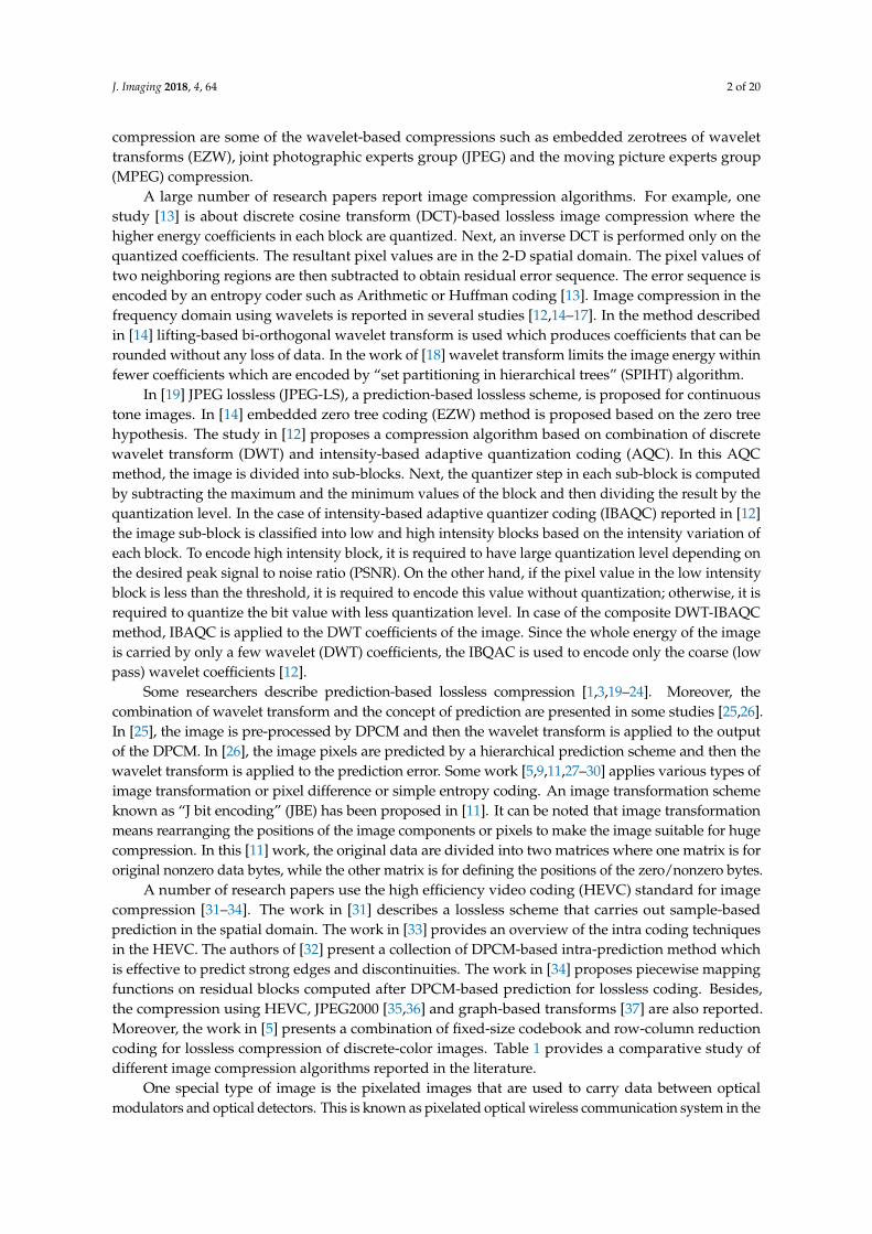
literature. Figure 1 illustrates one example of a pixelated system [38]. In such systems, a sequence of imageframes is transmitted by liquid crystal display (LCD) or light emitting diodes (LED) arrays. A smart-phonewith camera or an array of photodiode with imaging lens can be used as optical receivers [6–8]. Suchsystems have the potential to have huge data rates as there are millions of pixels on the transmitter screens.The images created on the optical transmitter are required to be within the field of view (FOV) of thereceiver imaging lens. Pixelated links can be used for secure data communication in banking and militaryapplications. For instance, pixelated systems can be useful at gatherings such as shopping malls, retailstore, trade shows, galleries, conferences, etc. where business cards, product videos, brochures, and photoscan be exchanged without the help of the Internet (www) connection. The storage of pixelated imagesmay be vital for offline processing. Since data are embedded within image pixels, the pixelated imagesmust be processed by lossless compression methods. Any amount of loss in image entropy may lead toloss in the embedded data. A very important feature of pixelated images is that a single intensity valuemade of pixel blocks contains a single data, and this value of intensity changes abruptly at the transitionof pixel blocks. This feature is not particularly exploited in the existing image compression techniques.Hence, none of the above-mentioned research reports are optimum for pixelated images as the specialfeatures of these images are yet to be exploited for compression. In fact, a new compression algorithm forpixelated images has been proposed by the authors of this paper in a very recent study [39]. This newalgorithm is termed as edge-based transformation and entropy coding (ETEC) having high compressionratio at moderate computation time. In this previous study [39], the ETEC method is evaluated for onlyfour pixelated images. This paper extends the study of ETEC method for fifty (50) different pixelatedimages. Moreover, a new algorithm termed as prediction-based transformation and entropy coding(PTEC) is proposed to overcome the limitations of computation time of ETEC. The main contributions ofthis paper can be summarized as follows:

(1) Providing a framework for ETEC method as a combination of JBE and entropy coding, and thenevaluating its effectiveness for compressing a wide range of pixelated images.

(2) Developing a new algorithm termed as PTEC by combining the aspects of hierarchical predictionapproach, JBE method, and entropy coding.

(3) Comparing the proposed ETEC and PTEC schemes with the existing compression techniques fora number of pixelated and non-pixelated standard images.

J. Imaging 2018, 4, x FOR PEER REVIEW 3 of 20

in the literature. Figure 1 illustrates one example of a pixelated system [38]. In such systems, a

sequence of image frames is transmitted by liquid crystal display (LCD) or light emitting diodes

(LED) arrays. A smart-phone with camera or an array of photodiode with imaging lens can be used

as optical receivers [6–8]. Such systems have the potential to have huge data rates as there are

millions of pixels on the transmitter screens. The images created on the optical transmitter are

required to be within the field of view (FOV) of the receiver imaging lens. Pixelated links can be used

for secure data communication in banking and military applications. For instance, pixelated systems

can be useful at gatherings such as shopping malls, retail store, trade shows, galleries, conferences,

etc. where business cards, product videos, brochures, and photos can be exchanged without the help

of the Internet (www) connection. The storage of pixelated images may be vital for offline

processing. Since data are embedded within image pixels, the pixelated images must be processed

by lossless compression methods. Any amount of loss in image entropy may lead to loss in the

embedded data. A very important feature of pixelated images is that a single intensity value made of

pixel blocks contains a single data, and this value of intensity changes abruptly at the transition of

pixel blocks. This feature is not particularly exploited in the existing image compression techniques.

Hence, none of the above-mentioned research reports are optimum for pixelated images as the

special features of these images are yet to be exploited for compression. In fact, a new compression

algorithm for pixelated images has been proposed by the authors of this paper in a very recent study

[39]. This new algorithm is termed as edge-based transformation and entropy coding (ETEC) having

high compression ratio at moderate computation time. In this previous study [39], the ETEC method

is evaluated for only four pixelated images. This paper extends the study of ETEC method for fifty

(50) different pixelated images. Moreover, a new algorithm termed as prediction-based

transformation and entropy coding (PTEC) is proposed to overcome the limitations of computation

time of ETEC. The main contributions of this paper can be summarized as follows:

(1) Providing a framework for ETEC method as a combination of JBE and entropy coding, and then

evaluating its effectiveness for compressing a wide range of pixelated images.

(2) Developing a new algorithm termed as PTEC by combining the aspects of hierarchical

prediction approach, JBE method, and entropy coding.

(3) Comparing the proposed ETEC and PTEC schemes with the existing compression techniques

for a number of pixelated and non-pixelated standard images.

Figure 1. Illustration of (a) a pixelated optical wireless communication system [38] (b) a transmitted

pixelated image.

(a)

(b)

Figure 1. Illustration of (a) a pixelated optical wireless communication system [38] (b) a transmittedpixelated image.

J. Imaging 2018, 4, 64 4 of 20

The rest of the paper is summarized as follows. Section 2 describes JPEG-LS, SPIHT, Huffmancoding, Arithmetic coding and other existing methods. Section 3 describes the new ETEC and PTECmethods. The results on different image compression methods are reported in Section 4. Finally,Section 5 presents the concluding remarks.

Table 1. Technical scenarios of few existing lossless and near lossless image compression algorithms.

Ref. No. PredictionBased

WaveletBased

PixelDifference

BasedDCT Entropy

Coding Image Encoder/Transformer Image Type HierarchicalApproach

[1] Yes No No No Yes PDT Dithering No[3] Yes No No No Yes No Continuous Yes[5] No No No No Yes Row-column reduction encoding Map images No[9] No No No No Yes LZW Continuous No

[11] No No No No Yes J bit encoding Continuous No[12] No Yes No No No AQC Continuous No[13] No No Yes Yes Yes No Continuous No[14] No Yes No No No Modified EZW Continuous No[15] No Yes No No No No All No[16] No Yes No No No No Color No[17] No Yes No No Yes No Continuous No[19] Yes No No No Yes No Continuous No[20] Yes No No No No H.264/AVC Hyper-spectral No[21] Yes No No No Yes Taylor series Continuous No[22] Yes No No No Yes AQC Continuous Yes[23] Yes No Yes No Yes S+P transform Continuous No[24] Yes No No No No LS based Natural No[25] Yes Yes No No Yes No Medical image No[26] Yes Yes No No No Color transform Color Yes[27] Yes No No Yes Yes Geometric, photometric transformation JPEG image No[28] No No No No Yes Dynamic bit reduction Continuous No[29] No No Block diff No No No Fractal No[30] No No No No No AQC (3-level) Continuous No[31] Yes No No Yes Yes residual coding All No[32] Yes No No No No residual coding All No[33] Yes No No No No residual coding All No[34] Yes No No No Yes residual coding All No[35] Yes Yes No No Yes residual coding All No[36] Yes Yes No No Yes Embedded block coding All No[37] Yes No No No Yes Graph based transforms All No

2. Existing Image Compression Techniques

The JPEG-LS compression algorithm is suited for continuous tone images. The compressionalgorithm consists of four main parts, which are fixed predictor, bias canceller or adaptive corrector,context modeler and entropy coder [19]. In JPEG-LS, the edge detection is performed by “median edgedetection” (MED) process [19]. JPEG-LS uses context modeling to measure the quantized gradientof surrounding image pixels. This context modeling of the predication error gives good resultsfor images with texture pattern. Next correction values are added to the prediction error, and theremaining or residual error is encoded by Golomb coding [40] scheme. SPIHT [18,41] is an advancedencoding technique based on progressive image coding. SPIHT uses a threshold and encodes the mostsignificant bit of the transformed image, followed by the application of increasing refinement. Thispaper considers SPIHT algorithm with lifting-based wavelet transform for 5/3 Le Gall wavelet filter.

Differential pulse code modulation (DPCM) [42] predictor can predict the current pixel basedon its neighboring pixels as mentioned in the JPEG-LS predictor. The subtraction of the current pixelintensity and the predictor output gives predictor error e. The quantizer quantizes the error valueusing suitable quantization level. In case of lossless compression, the quantized level is unity. Next, anentropy coding is performed to get the final bit streams. The predictor operator can be expressed bythe following equation

x̂s(i, j) = a ∗ I(i, j− 1) + b ∗ I(i− 1, j− 1) + c ∗ I(i− 1, j) + d ∗ I(i− 1, j + 1) + . . . . . . . (1)

where x̂s is predictor output, the terms a, b, c and d are constant, I is the intensity value and (x,y)represent the spatial indices of the pixels.

J. Imaging 2018, 4, 64 5 of 20

Arithmetic coding is an entropy coding used for lossless compression [43]. In this method, theinfrequently occurring symbols/characters are encoded with greater number of bits than frequentoccurring symbols/characters. An important feature of Arithmetic coding is that it encodes the fullinformation into a single long number and represents current information as a range. Huffmancoding [44] is basically a prefix coding method which assigns variable length codes to inputcharacters/symbols. In this scheme, the least frequently occurring character is assigned with thesmallest of the codes within a code table.

3. Proposed Algorithms

This section describes the recently proposed ETEC method and then proposes the PTEC method.

3.1. ETEC

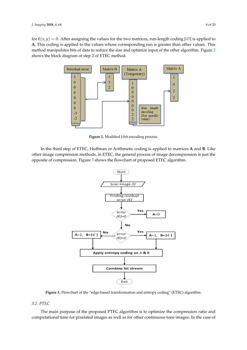
The study of ETEC is extended in this paper with a detailed analysis of the ETEC algorithm. It hasalready been mentioned in Section I that each pixel block of a pixelated image carries a single intensityvalue or a single piece of data. The pixel blocks have abrupt transition and thus have many directionaledges. The ETEC method can be described by three steps. In the first step, the special feature ofpixelated images is used to calculate a residual error € by using the following intensity gradient

∇I =

[gx

gy

]=

[∂I∂x∂I∂y

](2)

where ∂I/∂x is the derivative with respect to the x direction, ∂I/∂y is the derivative with respect to they direction, I is the intensity value and (x,y) represent the spatial indices of the pixels. The maximumchange of gradient between two co-ordinates represents the presence of edge either in the vertical orthe horizontal direction.

The edge pixels are responsible for the increase in the level of the residual error €. It can be notedthat for the presence of vertical edges, the value of € can be reduced to obtain the vertical intensitygradient. Similarly, for the presence of horizontal edges, the value of € can be reduced to obtain thehorizontal intensity gradient. In order to detect a strong edge, a threshold Th is applied to the residualerror in between the previous neighbors. If the previous residual error is greater than the threshold Th,then the present pixel I(x,y) is considered to be on the edge. So, the direction of gradient is changed.This can be mathematically described as:

if € =∂Ix

∂x> Th (3)

then € =∂Ix

∂x(4)

and if € =∂Iy

∂y> Th (5)

then € =∂Iy

∂y(6)

As long as the previous residual error is less than the threshold, i.e., € < Th, the scanning directionremains the same. After the whole scanning, the term € contains lower entropy compared to theoriginal image.

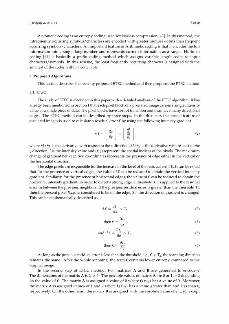
In the second step of ETEC method, two matrices A and B are generated to encode €.The dimensions of the matrix A is X × Y. The possible values of matrix A are 0 or 1 or 2 dependingon the value of €. The matrix A is assigned a value of 0 where €(x, y) has a value of 0. Moreover,the matrix A is assigned values of 1 and 2 where €(x, y) has a value greater than and less than 0,respectively. On the other hand, the matrix B is assigned with the absolute value of €(x, y), except

J. Imaging 2018, 4, 64 6 of 20

for €(x, y) = 0. After assigning the values for the two matrices, run-length coding [45] is applied toA. This coding is applied to the values whose corresponding run is greater than other values. Thismethod manipulates bits of data to reduce the size and optimize input of the other algorithm. Figure 2shows the block diagram of step 2 of ETEC method.

J. Imaging 2018, 4, x FOR PEER REVIEW 6 of 20

In the second step of ETEC method, two matrices A and B are generated to encode €. The

dimensions of the matrix A is X Y . The possible values of matrix A are 0 or 1 or 2 depending

on the value of € . The matrix A is assigned a value of 0 where x y€ , has a value of 0.

Moreover, the matrix A is assigned values of 1 and 2 where x y€ , has a value greater than and

less than 0, respectively. On the other hand, the matrix B is assigned with the absolute value of

x y€ , , except for x y€ , 0 . After assigning the values for the two matrices, run-length coding

[45] is applied to A . This coding is applied to the values whose corresponding run is greater than

other values. This method manipulates bits of data to reduce the size and optimize input of the other

algorithm. Figure 2 shows the block diagram of step 2 of ETEC method.

Figure 2. Modified J-bit encoding process.

In the third step of ETEC, Huffman or Arithmetic coding is applied to matrices A and B .

Like other image compression methods, in ETEC, the general process of image decompression is just

the opposite of compression. Figure 3 shows the flowchart of proposed ETEC algorithm.

Figure 3. Flowchart of the “edge-based transformation and entropy coding” (ETEC) algorithm.

Figure 2. Modified J-bit encoding process.

In the third step of ETEC, Huffman or Arithmetic coding is applied to matrices A and B. Likeother image compression methods, in ETEC, the general process of image decompression is just theopposite of compression. Figure 3 shows the flowchart of proposed ETEC algorithm.

J. Imaging 2018, 4, x FOR PEER REVIEW 6 of 20

In the second step of ETEC method, two matrices A and B are generated to encode €. The

dimensions of the matrix A is X Y . The possible values of matrix A are 0 or 1 or 2 depending

on the value of € . The matrix A is assigned a value of 0 where x y€ , has a value of 0.

Moreover, the matrix A is assigned values of 1 and 2 where x y€ , has a value greater than and

less than 0, respectively. On the other hand, the matrix B is assigned with the absolute value of

x y€ , , except for x y€ , 0 . After assigning the values for the two matrices, run-length coding

[45] is applied to A . This coding is applied to the values whose corresponding run is greater than

other values. This method manipulates bits of data to reduce the size and optimize input of the other

algorithm. Figure 2 shows the block diagram of step 2 of ETEC method.

Figure 2. Modified J-bit encoding process.

In the third step of ETEC, Huffman or Arithmetic coding is applied to matrices A and B .

Like other image compression methods, in ETEC, the general process of image decompression is just

the opposite of compression. Figure 3 shows the flowchart of proposed ETEC algorithm.

Figure 3. Flowchart of the “edge-based transformation and entropy coding” (ETEC) algorithm. Figure 3. Flowchart of the “edge-based transformation and entropy coding” (ETEC) algorithm.

3.2. PTEC

The main purpose of the proposed PTEC algorithm is to optimize the compression ratio andcomputational time for pixelated images as well as for other continuous tone images. In the case of

J. Imaging 2018, 4, 64 7 of 20

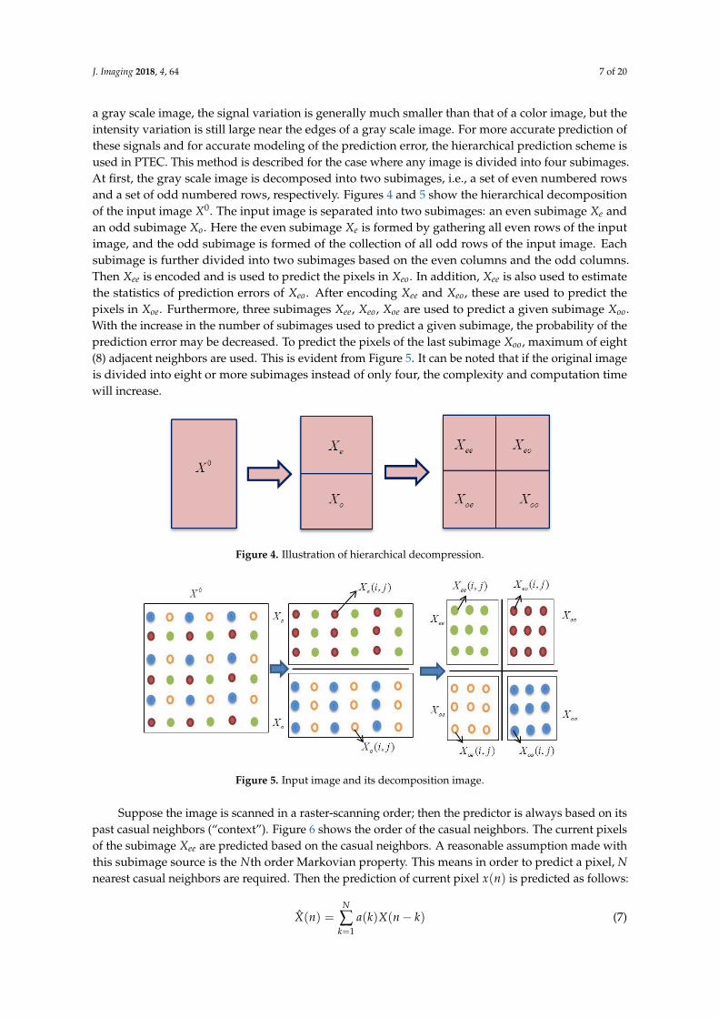
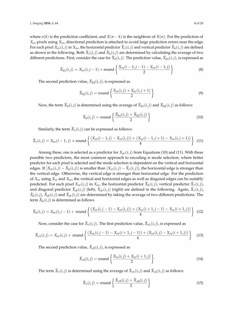
a gray scale image, the signal variation is generally much smaller than that of a color image, but theintensity variation is still large near the edges of a gray scale image. For more accurate prediction ofthese signals and for accurate modeling of the prediction error, the hierarchical prediction scheme isused in PTEC. This method is described for the case where any image is divided into four subimages.At first, the gray scale image is decomposed into two subimages, i.e., a set of even numbered rowsand a set of odd numbered rows, respectively. Figures 4 and 5 show the hierarchical decompositionof the input image X0. The input image is separated into two subimages: an even subimage Xe andan odd subimage Xo. Here the even subimage Xe is formed by gathering all even rows of the inputimage, and the odd subimage is formed of the collection of all odd rows of the input image. Eachsubimage is further divided into two subimages based on the even columns and the odd columns.Then Xee is encoded and is used to predict the pixels in Xeo. In addition, Xee is also used to estimatethe statistics of prediction errors of Xeo. After encoding Xee and Xeo, these are used to predict thepixels in Xoe. Furthermore, three subimages Xee, Xeo, Xoe are used to predict a given subimage Xoo.With the increase in the number of subimages used to predict a given subimage, the probability of theprediction error may be decreased. To predict the pixels of the last subimage Xoo, maximum of eight(8) adjacent neighbors are used. This is evident from Figure 5. It can be noted that if the original imageis divided into eight or more subimages instead of only four, the complexity and computation timewill increase.

J. Imaging 2018, 4, x FOR PEER REVIEW 7 of 20

3.2. PTEC

The main purpose of the proposed PTEC algorithm is to optimize the compression ratio and

computational time for pixelated images as well as for other continuous tone images. In the case of a

gray scale image, the signal variation is generally much smaller than that of a color image, but the

intensity variation is still large near the edges of a gray scale image. For more accurate prediction of

these signals and for accurate modeling of the prediction error, the hierarchical prediction scheme is

used in PTEC. This method is described for the case where any image is divided into four

subimages. At first, the gray scale image is decomposed into two subimages, i.e., a set of even

numbered rows and a set of odd numbered rows, respectively. Figures 4 and 5 show the hierarchical

decomposition of the input image X0 . The input image is separated into two subimages: an even

subimage e

X and an odd subimage o

X . Here the even subimage e

X is formed by gathering all

even rows of the input image, and the odd subimage is formed of the collection of all odd rows of the

input image. Each subimage is further divided into two subimages based on the even columns and

the odd columns. Then ee

X is encoded and is used to predict the pixels in eo

X . In addition, ee

X is

also used to estimate the statistics of prediction errors of eo

X . After encoding ee

X and eo

X , these

are used to predict the pixels in oe

X . Furthermore, three subimages ee

X , eo

X , oe

X are used to

predict a given subimage oo

X . With the increase in the number of subimages used to predict a given

subimage, the probability of the prediction error may be decreased. To predict the pixels of the last

subimage oo

X , maximum of eight (8) adjacent neighbors are used. This is evident from Figure 5. It

can be noted that if the original image is divided into eight or more subimages instead of only four,

the complexity and computation time will increase.

Figure 4. Illustration of hierarchical decompression.

Figure 5. Input image and its decomposition image.

Suppose the image is scanned in a raster-scanning order; then the predictor is always based on

its past casual neighbors (“context”). Figure 6 shows the order of the casual neighbors. The current

pixels of the subimage eeX are predicted based on the casual neighbors. A reasonable assumption

made with this subimage source is the thN order Markovian property. This means in order to

Figure 4. Illustration of hierarchical decompression.

J. Imaging 2018, 4, x FOR PEER REVIEW 7 of 20

3.2. PTEC

The main purpose of the proposed PTEC algorithm is to optimize the compression ratio and

computational time for pixelated images as well as for other continuous tone images. In the case of a

gray scale image, the signal variation is generally much smaller than that of a color image, but the

intensity variation is still large near the edges of a gray scale image. For more accurate prediction of

these signals and for accurate modeling of the prediction error, the hierarchical prediction scheme is

used in PTEC. This method is described for the case where any image is divided into four

subimages. At first, the gray scale image is decomposed into two subimages, i.e., a set of even

numbered rows and a set of odd numbered rows, respectively. Figures 4 and 5 show the hierarchical

decomposition of the input image X0 . The input image is separated into two subimages: an even

subimage e

X and an odd subimage o

X . Here the even subimage e

X is formed by gathering all

even rows of the input image, and the odd subimage is formed of the collection of all odd rows of the

input image. Each subimage is further divided into two subimages based on the even columns and

the odd columns. Then ee

X is encoded and is used to predict the pixels in eo

X . In addition, ee

X is

also used to estimate the statistics of prediction errors of eo

X . After encoding ee

X and eo

X , these

are used to predict the pixels in oe

X . Furthermore, three subimages ee

X , eo

X , oe

X are used to

predict a given subimage oo

X . With the increase in the number of subimages used to predict a given

subimage, the probability of the prediction error may be decreased. To predict the pixels of the last

subimage oo

X , maximum of eight (8) adjacent neighbors are used. This is evident from Figure 5. It

can be noted that if the original image is divided into eight or more subimages instead of only four,

the complexity and computation time will increase.

Figure 4. Illustration of hierarchical decompression.

Figure 5. Input image and its decomposition image.

Suppose the image is scanned in a raster-scanning order; then the predictor is always based on

its past casual neighbors (“context”). Figure 6 shows the order of the casual neighbors. The current

pixels of the subimage eeX are predicted based on the casual neighbors. A reasonable assumption

made with this subimage source is the thN order Markovian property. This means in order to

Figure 5. Input image and its decomposition image.

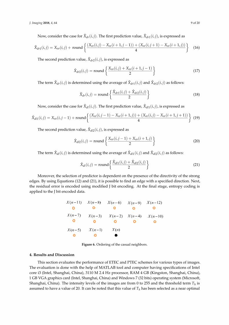
Suppose the image is scanned in a raster-scanning order; then the predictor is always based on itspast casual neighbors (“context”). Figure 6 shows the order of the casual neighbors. The current pixelsof the subimage Xee are predicted based on the casual neighbors. A reasonable assumption made withthis subimage source is the Nth order Markovian property. This means in order to predict a pixel, Nnearest casual neighbors are required. Then the prediction of current pixel x(n) is predicted as follows:

X̂(n) =N

∑k=1

a(k)X(n− k) (7)

J. Imaging 2018, 4, 64 8 of 20

where a(k) is the prediction coefficient, and X(n− k) is the neighbors of X(n). For the prediction ofXeo pixels using Xee, directional prediction is attached to avoid large prediction errors near the edge.For each pixel Xeo(i, j) in Xeo, the horizontal predictor X̂v(i, j) and vertical predictor X̂h(i, j) are definedas shown in the following. Both X̂v(i, j) and X̂h(i, j) are determined by calculating the average of twodifferent predictions. First, consider the case for X̂h(i, j). The prediction value, X̂h1(i, j), is expressed as

X̂h1(i, j) = Xeo(i, j− 1) + round{

Xeo(i− 1, j− 1)− Xeo(i− 1, j)2

}(8)

The second prediction value, X̂h2(i, j), is expressed as

X̂h2(i, j) = round{

Xee(i, j) + Xee(i, j + 1)2

}(9)

Now, the term X̂h(i, j) is determined using the average of X̂h1(i, j) and X̂h2(i, j) as follows:

X̂h(i, j) = round{

X̂h1(i, j) + X̂h2(i, j)2

}(10)

Similarly, the term X̂v(i, j) can be expressed as follows:

X̂v(i, j) = Xeo(i− 1, j) + round{(Xee(i− 1, j)− Xee(i, j)) + (Xee(i− 1, j + 1)− Xee(i, j + 1))

4

}(11)

Among these, one is selected as a predictor for Xeo(i, j) from Equations (10) and (11). With thesepossible two predictors, the most common approach to encoding is mode selection; where betterpredictor for each pixel is selected and the mode selection is dependent on the vertical and horizontaledges. If

∣∣Xeo(i, j)− X̂h(i, j)∣∣ is smaller than

∣∣Xeo(i, j)− X̂v(i, j)∣∣, the horizontal edge is stronger than

the vertical edge. Otherwise, the vertical edge is stronger than horizontal edge. For the predictionof Xoe using Xee and Xeo, the vertical and horizontal edges as well as diagonal edges can be suitablypredicted. For each pixel Xoe(i, j) in Xoe, the horizontal predictor X̂h(i, j), vertical predictor X̂v(i, j),and diagonal predictor X̂dl(i, j) (left), X̂dr(i, j) (right) are defined in the following. Again, X̂v(i, j),X̂h(i, j), X̂dl(i, j) and X̂dr(i, j) are determined by taking the average of two different predictions. Theterm X̂h(i, j) is determined as follows

X̂h(i, j) = Xoe(i, j− 1) + round{(Xee(i, j− 1)− Xee(i, j)) + (Xee(i + 1, j− 1)− Xee(i + 1, j))

4

}(12)

Now, consider the case for X̂v(i, j). The first prediction value, X̂v1(i, j), is expressed as

X̂v1(i, j) = Xee(i, j) + round{(Xeo(i, j− 1)− Xeo(i + 1, j− 1)) + (Xeo(i, j)− Xeo(i + 1, j))

4

}(13)

The second prediction value, X̂v2(i, j), is expressed as

X̂v2(i, j) = round{

Xee(i, j) + Xee(i + 1, j)2

}(14)

The term X̂v(i, j) is determined using the average of X̂v1(i, j) and X̂v2(i, j) as follows:

X̂v(i, j) = round{

X̂v3(i, j) + X̂v4(i, j)2

}(15)

J. Imaging 2018, 4, 64 9 of 20

Now, consider the case for X̂dr(i, j). The first prediction value, X̂dr1(i, j), is expressed as

X̂dr1(i, j) = Xeo(i, j) + round{(Xee(i, j)− Xee(i + 1, j− 1)) + (Xee(i, j + 1)− Xee(i + 1, j))

4

}(16)

The second prediction value, X̂dr2(i, j), is expressed as

X̂dr2(i, j) = round{

Xeo(i, j) + Xeo(i + 1, j− 1)2

}(17)

The term X̂dr(i, j) is determined using the average of X̂dr1(i, j) and X̂dr2(i, j) as follows:

X̂dr(i, j) = round{

X̂dr1(i, j) + X̂dr2(i, j)2

}(18)

Now, consider the case for X̂dl(i, j). The first prediction value, X̂dl1(i, j), is expressed as

X̂dl1(i, j) = Xeo(i, j− 1) + round{(Xee(i, j− 1)− Xee(i + 1, j)) + (Xee(i, j)− Xee(i + 1, j + 1))

4

}(19)

The second prediction value, X̂dl2(i, j), is expressed as

X̂dl2(i, j) = round{

Xeo(i, j− 1) + Xeo(i + 1, j)2

}(20)

The term X̂dl(i, j) is determined using the average of X̂dl1(i, j) and X̂dl2(i, j) as follows:

X̂dl(i, j) = round{

X̂dl1(i, j) + X̂dl2(i, j)2

}(21)

Moreover, the selection of predictor is dependent on the presence of the directivity of the strongedges. By using Equations (12) and (21), it is possible to find an edge with a specified direction. Next,the residual error is encoded using modified J bit encoding. At the final stage, entropy coding isapplied to the J bit encoded data.

J. Imaging 2018, 4, x FOR PEER REVIEW 9 of 20

The second prediction value, v

X i j2

ˆ ( , ) , is expressed as

ee eev

X i j X i jX i j

2

( , ) ( 1, )ˆ ( , ) round2

(14)

The term v

X i jˆ ( , ) is determined using the average of v

X i j1

ˆ ( , ) and v

X i j2

ˆ ( , ) as follows:

3 4ˆ ˆ( , ) ( , )ˆ ( , ) round

2v v

v

X i j X i jX i j (15)

Now, consider the case for dr

X i jˆ ( , ) . The first prediction value, dr

X i j1

ˆ ( , ) , is expressed as

ee ee ee ee

dr eo

X i j X i j X i j X i jX i j X i j

1

( , ) ( 1, 1) ( , 1) ( 1, )ˆ ( , ) ( , ) round

4 (16)

The second prediction value, dr

X i j2

ˆ ( , ) , is expressed as

eo eodr

X i j X i jX i j

2

( , ) ( 1, 1)ˆ ( , ) round2

(17)

The term dr

X i jˆ ( , ) is determined using the average of dr

X i j1

ˆ ( , ) and dr

X i j2

ˆ ( , ) as follows:

1 2ˆ ˆ( , ) ( , )ˆ ( , ) round

2dr dr

dr

X i j X i jX i j (18)

Now, consider the case for dl

X i jˆ ( , ) . The first prediction value, dl

X i j1

ˆ ( , ) , is expressed as

ee ee ee ee

dl eo

X i j X i j X i j X i jX i j X i j

1

( , 1) ( 1, ) ( , ) ( 1, 1)ˆ ( , ) ( , 1) round

4 (19)

The second prediction value, dl

X i j2

ˆ ( , ) , is expressed as

eo eodl

X i j X i jX i j

2

( , 1) ( 1, )ˆ ( , ) round2

(20)

The term dl

X i jˆ ( , ) is determined using the average of dl

X i j1

ˆ ( , ) and dl

X i j2

ˆ ( , ) as follows:

1 2ˆ ˆ( , ) ( , )ˆ ( , ) round

2dl dl

dl

X i j X i jX i j (21)

Moreover, the selection of predictor is dependent on the presence of the directivity of the strong

edges. By using Equations (12) and (21), it is possible to find an edge with a specified direction. Next,

the residual error is encoded using modified J bit encoding. At the final stage, entropy coding is

applied to the J bit encoded data.

Figure 6. Ordering of the casual neighbors.

Figure 6. Ordering of the casual neighbors.

4. Results and Discussion

This section evaluates the performance of ETEC and PTEC schemes for various types of images.The evaluation is done with the help of MATLAB tool and computer having specifications of Intelcore i3 (Intel, Shanghai, China), 3110 M 2.4 Hz processor, RAM 4 GB (Kingston, Shanghai, China),1 GB VGA graphics card (Intel, Shanghai, China) and Windows 7 (32 bits) operating system (Microsoft,Shanghai, China). The intensity levels of the images are from 0 to 255 and the threshold term Th isassumed to have a value of 20. It can be noted that this value of Th has been selected as a near optimal

J. Imaging 2018, 4, 64 10 of 20

value. Since a high value of Th may not recognize some edges in the images, whereas low values of Thmay unnecessary consider any small transition as an edge

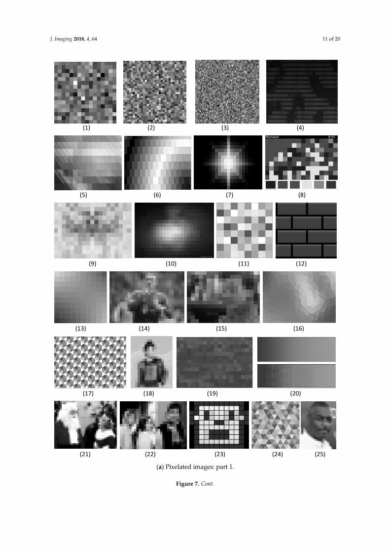
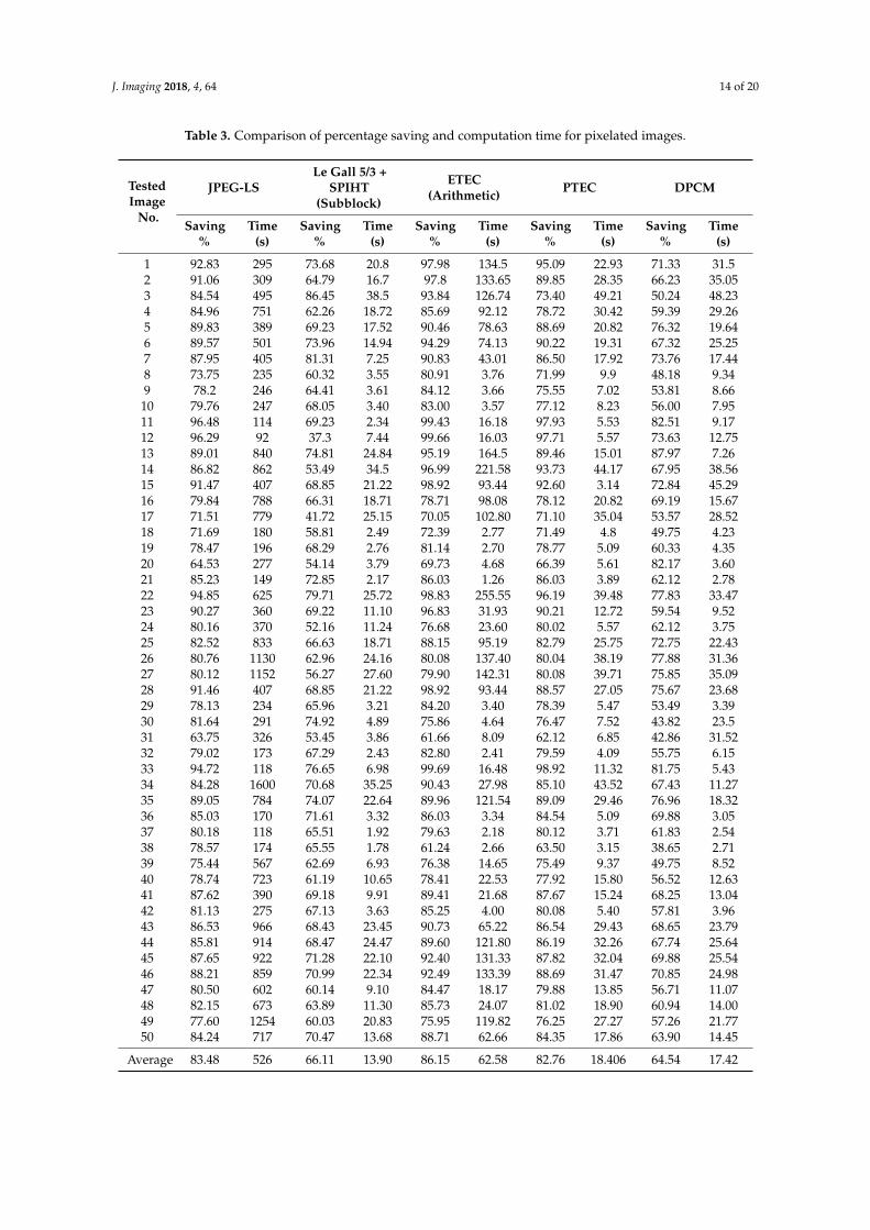
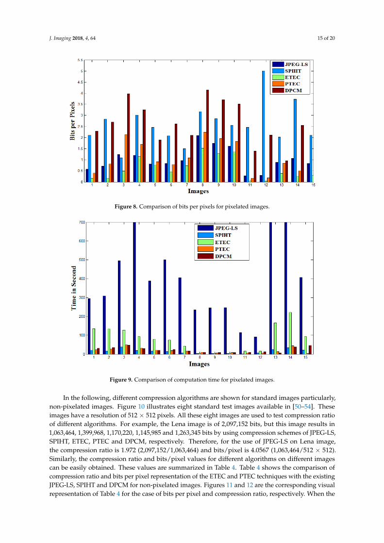
Figure 7 shows 50 different types of pixelated images used for evaluating the compressionalgorithms. Some of these images are created using MATLAB tool, and the remaining ones areavailable in [46–49]. Both Figure 7a,b have 25 images each. These images are made of different pixelblocks and each block is of different pixel sizes. Each pixel block has uniform intensity level. In somecases, a pixelated image may have very small pixel block or no block (each pixel block made of onepixel only). A number of metrics such as compression ratio, bits per pixel, saving percentage [28], andcomputation time are considered for comparing the algorithms. It can be noted that in this study thecompression ratio is defined as the ratio of the size of the original image to the compressed image.Moreover, the saving percentage parameter is the difference between the original image and thecompressed image as a percentage of the original image. Mathematically, the compression ratio isC1/C2, and the saving percentage is (1− C2/C1) where C1 and C2 are the size of the original imageand the compressed image, respectively. The bit per pixel parameter is obtained by dividing theimage size (in bytes) by the number of pixels in the compressed image. The computation time is thetotal amount of time required to perform the image compression using MATLAB tool with the givencomputer specified earlier in this section.

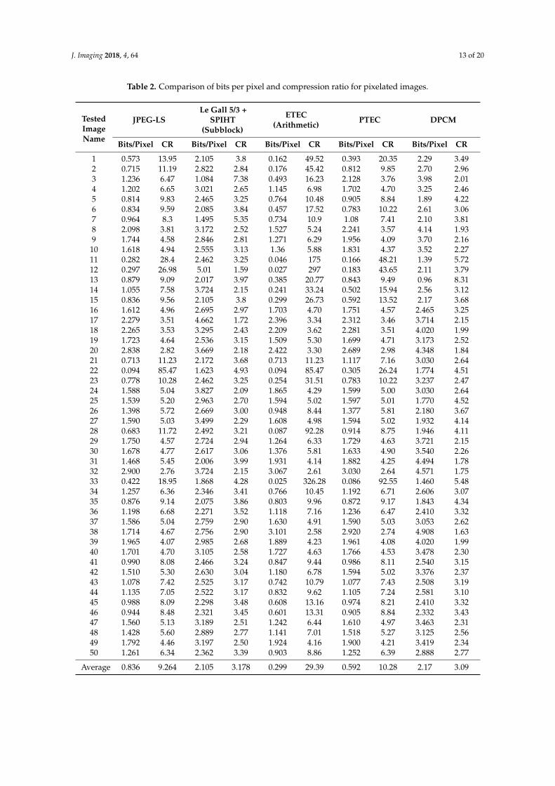
First, consider the compression ratio (denoted as CR) and bits/pixel parameters. In Table 2,compression ratio and bits/pixel metrics are compared for the proposed ETEC and PTEC techniqueswith the existing JPEG-LS, SPIHT, and DPCM methods. The comparison is done for the 50 pixelatedimages illustrated in Figure 7. The bits per pixel parameter of the first 15 images are plotted in Figure 8for the proposed and existing compression algorithms. Now consider the saving percentage andcomputation time. Table 3 represents the percentage saving and computation time for the case of those50 images. The computation time in seconds is also plotted for the first 15 images in Figure 9. It canbe seen from Table 2 that for the pixelated images, the average bits per pixel for ETEC (0.299) andPTEC (0.592) are lower (better) than the existing JPEG-LS (0.836), SPIHT (2.105) and DPCM (2.17).Table 2 shows that the average compression ratio of ETEC (29.39) and PTEC (10.28) are better thanSPIHT (3.178) and JPEG-LS (9.264) and DPCM (3.09). Table 2 also shows that the compression ratio ofPTEC is not always better than JPEG-LS for all the 50 pixelated images. In particular, PTEC has bettercompression than JPEG-LS for pixelated images having large pixel blocks. For small pixel blocks, thecompression performance of PTEC is worse than JPEG-LS. This is because of the hierarchical predictionof PTEC. In case of small pixel block images, the prediction error for the first subimage is very high dueto the high randomness of pixel intensity. For large pixel block images, this problem is significantlyreduced. Table 3 indicates that the computational time of ETEC (62.58 s) is worse than SPIHT (13.9 s),but better than JPEG-LS (526 s) and DPCM (17.48 s). Furthermore, PTEC method has a computationtime of 18.406 s which is much better than ETEC (62.58 s) and comparable to SPIHT (13.9 s). So, forpixelated images and for the case where both compression and computation time are important, PTECmay be more suitable than ETEC, SPIHT, JPEG-LS and DPCM.

J. Imaging 2018, 4, 64 11 of 20

J. Imaging 2018, 4, x FOR PEER REVIEW 11 of 20

(a) Pixelated images: part 1.

(1) (2) (3) (4)

(5) (6) (7) (8)

(9) (10) (11) (12)

(13) (14) (15) (16)

(17) (18) (19) (20)

(21) (22) (23) (24) (25)

Figure 7. Cont.

J. Imaging 2018, 4, 64 12 of 20

J. Imaging 2018, 4, x FOR PEER REVIEW 12 of 20

(b) Pixelated images: part 2.

Figure 7. Tested pixelated images [46–49].

(26) (27) (28) (29) (30)

(31) (32) (33) (34)

(35) (36) (37) (38)

(39) (40) (41) (42)

(43) (44) (45) (46)

(47) (48) (49) (50)

Figure 7. Tested pixelated images [46–49].

J. Imaging 2018, 4, 64 13 of 20

Table 2. Comparison of bits per pixel and compression ratio for pixelated images.

TestedImageName

JPEG-LSLe Gall 5/3 +

SPIHT(Subblock)

ETEC(Arithmetic) PTEC DPCM

Bits/Pixel CR Bits/Pixel CR Bits/Pixel CR Bits/Pixel CR Bits/Pixel CR

1 0.573 13.95 2.105 3.8 0.162 49.52 0.393 20.35 2.29 3.492 0.715 11.19 2.822 2.84 0.176 45.42 0.812 9.85 2.70 2.963 1.236 6.47 1.084 7.38 0.493 16.23 2.128 3.76 3.98 2.014 1.202 6.65 3.021 2.65 1.145 6.98 1.702 4.70 3.25 2.465 0.814 9.83 2.465 3.25 0.764 10.48 0.905 8.84 1.89 4.226 0.834 9.59 2.085 3.84 0.457 17.52 0.783 10.22 2.61 3.067 0.964 8.3 1.495 5.35 0.734 10.9 1.08 7.41 2.10 3.818 2.098 3.81 3.172 2.52 1.527 5.24 2.241 3.57 4.14 1.939 1.744 4.58 2.846 2.81 1.271 6.29 1.956 4.09 3.70 2.16

10 1.618 4.94 2.555 3.13 1.36 5.88 1.831 4.37 3.52 2.2711 0.282 28.4 2.462 3.25 0.046 175 0.166 48.21 1.39 5.7212 0.297 26.98 5.01 1.59 0.027 297 0.183 43.65 2.11 3.7913 0.879 9.09 2.017 3.97 0.385 20.77 0.843 9.49 0.96 8.3114 1.055 7.58 3.724 2.15 0.241 33.24 0.502 15.94 2.56 3.1215 0.836 9.56 2.105 3.8 0.299 26.73 0.592 13.52 2.17 3.6816 1.612 4.96 2.695 2.97 1.703 4.70 1.751 4.57 2.465 3.2517 2.279 3.51 4.662 1.72 2.396 3.34 2.312 3.46 3.714 2.1518 2.265 3.53 3.295 2.43 2.209 3.62 2.281 3.51 4.020 1.9919 1.723 4.64 2.536 3.15 1.509 5.30 1.699 4.71 3.173 2.5220 2.838 2.82 3.669 2.18 2.422 3.30 2.689 2.98 4.348 1.8421 0.713 11.23 2.172 3.68 0.713 11.23 1.117 7.16 3.030 2.6422 0.094 85.47 1.623 4.93 0.094 85.47 0.305 26.24 1.774 4.5123 0.778 10.28 2.462 3.25 0.254 31.51 0.783 10.22 3.237 2.4724 1.588 5.04 3.827 2.09 1.865 4.29 1.599 5.00 3.030 2.6425 1.539 5.20 2.963 2.70 1.594 5.02 1.597 5.01 1.770 4.5226 1.398 5.72 2.669 3.00 0.948 8.44 1.377 5.81 2.180 3.6727 1.590 5.03 3.499 2.29 1.608 4.98 1.594 5.02 1.932 4.1428 0.683 11.72 2.492 3.21 0.087 92.28 0.914 8.75 1.946 4.1129 1.750 4.57 2.724 2.94 1.264 6.33 1.729 4.63 3.721 2.1530 1.678 4.77 2.617 3.06 1.376 5.81 1.633 4.90 3.540 2.2631 1.468 5.45 2.006 3.99 1.931 4.14 1.882 4.25 4.494 1.7832 2.900 2.76 3.724 2.15 3.067 2.61 3.030 2.64 4.571 1.7533 0.422 18.95 1.868 4.28 0.025 326.28 0.086 92.55 1.460 5.4834 1.257 6.36 2.346 3.41 0.766 10.45 1.192 6.71 2.606 3.0735 0.876 9.14 2.075 3.86 0.803 9.96 0.872 9.17 1.843 4.3436 1.198 6.68 2.271 3.52 1.118 7.16 1.236 6.47 2.410 3.3237 1.586 5.04 2.759 2.90 1.630 4.91 1.590 5.03 3.053 2.6238 1.714 4.67 2.756 2.90 3.101 2.58 2.920 2.74 4.908 1.6339 1.965 4.07 2.985 2.68 1.889 4.23 1.961 4.08 4.020 1.9940 1.701 4.70 3.105 2.58 1.727 4.63 1.766 4.53 3.478 2.3041 0.990 8.08 2.466 3.24 0.847 9.44 0.986 8.11 2.540 3.1542 1.510 5.30 2.630 3.04 1.180 6.78 1.594 5.02 3.376 2.3743 1.078 7.42 2.525 3.17 0.742 10.79 1.077 7.43 2.508 3.1944 1.135 7.05 2.522 3.17 0.832 9.62 1.105 7.24 2.581 3.1045 0.988 8.09 2.298 3.48 0.608 13.16 0.974 8.21 2.410 3.3246 0.944 8.48 2.321 3.45 0.601 13.31 0.905 8.84 2.332 3.4347 1.560 5.13 3.189 2.51 1.242 6.44 1.610 4.97 3.463 2.3148 1.428 5.60 2.889 2.77 1.141 7.01 1.518 5.27 3.125 2.5649 1.792 4.46 3.197 2.50 1.924 4.16 1.900 4.21 3.419 2.3450 1.261 6.34 2.362 3.39 0.903 8.86 1.252 6.39 2.888 2.77

Average 0.836 9.264 2.105 3.178 0.299 29.39 0.592 10.28 2.17 3.09

J. Imaging 2018, 4, 64 14 of 20

Table 3. Comparison of percentage saving and computation time for pixelated images.

TestedImage

No.

JPEG-LSLe Gall 5/3 +

SPIHT(Subblock)

ETEC(Arithmetic) PTEC DPCM

Saving%

Time(s)

Saving%

Time(s)

Saving%

Time(s)

Saving%

Time(s)

Saving%

Time(s)

1 92.83 295 73.68 20.8 97.98 134.5 95.09 22.93 71.33 31.52 91.06 309 64.79 16.7 97.8 133.65 89.85 28.35 66.23 35.053 84.54 495 86.45 38.5 93.84 126.74 73.40 49.21 50.24 48.234 84.96 751 62.26 18.72 85.69 92.12 78.72 30.42 59.39 29.265 89.83 389 69.23 17.52 90.46 78.63 88.69 20.82 76.32 19.646 89.57 501 73.96 14.94 94.29 74.13 90.22 19.31 67.32 25.257 87.95 405 81.31 7.25 90.83 43.01 86.50 17.92 73.76 17.448 73.75 235 60.32 3.55 80.91 3.76 71.99 9.9 48.18 9.349 78.2 246 64.41 3.61 84.12 3.66 75.55 7.02 53.81 8.66

10 79.76 247 68.05 3.40 83.00 3.57 77.12 8.23 56.00 7.9511 96.48 114 69.23 2.34 99.43 16.18 97.93 5.53 82.51 9.1712 96.29 92 37.3 7.44 99.66 16.03 97.71 5.57 73.63 12.7513 89.01 840 74.81 24.84 95.19 164.5 89.46 15.01 87.97 7.2614 86.82 862 53.49 34.5 96.99 221.58 93.73 44.17 67.95 38.5615 91.47 407 68.85 21.22 98.92 93.44 92.60 3.14 72.84 45.2916 79.84 788 66.31 18.71 78.71 98.08 78.12 20.82 69.19 15.6717 71.51 779 41.72 25.15 70.05 102.80 71.10 35.04 53.57 28.5218 71.69 180 58.81 2.49 72.39 2.77 71.49 4.8 49.75 4.2319 78.47 196 68.29 2.76 81.14 2.70 78.77 5.09 60.33 4.3520 64.53 277 54.14 3.79 69.73 4.68 66.39 5.61 82.17 3.6021 85.23 149 72.85 2.17 86.03 1.26 86.03 3.89 62.12 2.7822 94.85 625 79.71 25.72 98.83 255.55 96.19 39.48 77.83 33.4723 90.27 360 69.22 11.10 96.83 31.93 90.21 12.72 59.54 9.5224 80.16 370 52.16 11.24 76.68 23.60 80.02 5.57 62.12 3.7525 82.52 833 66.63 18.71 88.15 95.19 82.79 25.75 72.75 22.4326 80.76 1130 62.96 24.16 80.08 137.40 80.04 38.19 77.88 31.3627 80.12 1152 56.27 27.60 79.90 142.31 80.08 39.71 75.85 35.0928 91.46 407 68.85 21.22 98.92 93.44 88.57 27.05 75.67 23.6829 78.13 234 65.96 3.21 84.20 3.40 78.39 5.47 53.49 3.3930 81.64 291 74.92 4.89 75.86 4.64 76.47 7.52 43.82 23.531 63.75 326 53.45 3.86 61.66 8.09 62.12 6.85 42.86 31.5232 79.02 173 67.29 2.43 82.80 2.41 79.59 4.09 55.75 6.1533 94.72 118 76.65 6.98 99.69 16.48 98.92 11.32 81.75 5.4334 84.28 1600 70.68 35.25 90.43 27.98 85.10 43.52 67.43 11.2735 89.05 784 74.07 22.64 89.96 121.54 89.09 29.46 76.96 18.3236 85.03 170 71.61 3.32 86.03 3.34 84.54 5.09 69.88 3.0537 80.18 118 65.51 1.92 79.63 2.18 80.12 3.71 61.83 2.5438 78.57 174 65.55 1.78 61.24 2.66 63.50 3.15 38.65 2.7139 75.44 567 62.69 6.93 76.38 14.65 75.49 9.37 49.75 8.5240 78.74 723 61.19 10.65 78.41 22.53 77.92 15.80 56.52 12.6341 87.62 390 69.18 9.91 89.41 21.68 87.67 15.24 68.25 13.0442 81.13 275 67.13 3.63 85.25 4.00 80.08 5.40 57.81 3.9643 86.53 966 68.43 23.45 90.73 65.22 86.54 29.43 68.65 23.7944 85.81 914 68.47 24.47 89.60 121.80 86.19 32.26 67.74 25.6445 87.65 922 71.28 22.10 92.40 131.33 87.82 32.04 69.88 25.5446 88.21 859 70.99 22.34 92.49 133.39 88.69 31.47 70.85 24.9847 80.50 602 60.14 9.10 84.47 18.17 79.88 13.85 56.71 11.0748 82.15 673 63.89 11.30 85.73 24.07 81.02 18.90 60.94 14.0049 77.60 1254 60.03 20.83 75.95 119.82 76.25 27.27 57.26 21.7750 84.24 717 70.47 13.68 88.71 62.66 84.35 17.86 63.90 14.45

Average 83.48 526 66.11 13.90 86.15 62.58 82.76 18.406 64.54 17.42

J. Imaging 2018, 4, 64 15 of 20J. Imaging 2018, 4, x FOR PEER REVIEW 15 of 20

Figure 8. Comparison of bits per pixels for pixelated images.

Figure 9. Comparison of computation time for pixelated images.

In the following, different compression algorithms are shown for standard images particularly,

non-pixelated images. Figure 10 illustrates eight standard test images available in [50–54]. These

images have a resolution of 512 × 512 pixels. All these eight images are used to test compression

ratio of different algorithms. For example, the Lena image is of 2,097,152 bits, but this image results

in 1,063,464, 1,399,968, 1,170,220, 1,145,985 and 1,263,345 bits by using compression schemes of

JPEG-LS, SPIHT, ETEC, PTEC and DPCM, respectively. Therefore, for the use of JPEG-LS on Lena

image, the compression ratio is 1.972 (2,097,152/1,063,464) and bits/pixel is 4.0567 (1,063,464/512 ×

512). Similarly, the compression ratio and bits/pixel values for different algorithms on different

images can be easily obtained. These values are summarized in Table 4. Table 4 shows the

comparison of compression ratio and bits per pixel representation of the ETEC and PTEC

techniques with the existing JPEG-LS, SPIHT and DPCM for non-pixelated images. Figures 11 and

12 are the corresponding visual representation of Table 4 for the case of bits per pixel and

compression ratio, respectively. When the average compression ratio is considered, PTEC (2.06) is

better than SPIHT (1.76), ETEC (1.93) and DPCM (1.72), but worse than JPEG-LS (2.16). Similarly,

PTEC is better than SPIHT, ETEC and DPCM but worse than JPEG-LS in terms of average bits/pixel

Figure 8. Comparison of bits per pixels for pixelated images.

J. Imaging 2018, 4, x FOR PEER REVIEW 15 of 20

Figure 8. Comparison of bits per pixels for pixelated images.

Figure 9. Comparison of computation time for pixelated images.

In the following, different compression algorithms are shown for standard images particularly,

non-pixelated images. Figure 10 illustrates eight standard test images available in [50–54]. These

images have a resolution of 512 × 512 pixels. All these eight images are used to test compression

ratio of different algorithms. For example, the Lena image is of 2,097,152 bits, but this image results

in 1,063,464, 1,399,968, 1,170,220, 1,145,985 and 1,263,345 bits by using compression schemes of

JPEG-LS, SPIHT, ETEC, PTEC and DPCM, respectively. Therefore, for the use of JPEG-LS on Lena

image, the compression ratio is 1.972 (2,097,152/1,063,464) and bits/pixel is 4.0567 (1,063,464/512 ×

512). Similarly, the compression ratio and bits/pixel values for different algorithms on different

images can be easily obtained. These values are summarized in Table 4. Table 4 shows the

comparison of compression ratio and bits per pixel representation of the ETEC and PTEC

techniques with the existing JPEG-LS, SPIHT and DPCM for non-pixelated images. Figures 11 and

12 are the corresponding visual representation of Table 4 for the case of bits per pixel and

compression ratio, respectively. When the average compression ratio is considered, PTEC (2.06) is

better than SPIHT (1.76), ETEC (1.93) and DPCM (1.72), but worse than JPEG-LS (2.16). Similarly,

PTEC is better than SPIHT, ETEC and DPCM but worse than JPEG-LS in terms of average bits/pixel

Figure 9. Comparison of computation time for pixelated images.

In the following, different compression algorithms are shown for standard images particularly,non-pixelated images. Figure 10 illustrates eight standard test images available in [50–54]. Theseimages have a resolution of 512 × 512 pixels. All these eight images are used to test compression ratioof different algorithms. For example, the Lena image is of 2,097,152 bits, but this image results in1,063,464, 1,399,968, 1,170,220, 1,145,985 and 1,263,345 bits by using compression schemes of JPEG-LS,SPIHT, ETEC, PTEC and DPCM, respectively. Therefore, for the use of JPEG-LS on Lena image,the compression ratio is 1.972 (2,097,152/1,063,464) and bits/pixel is 4.0567 (1,063,464/512 × 512).Similarly, the compression ratio and bits/pixel values for different algorithms on different imagescan be easily obtained. These values are summarized in Table 4. Table 4 shows the comparison ofcompression ratio and bits per pixel representation of the ETEC and PTEC techniques with the existingJPEG-LS, SPIHT and DPCM for non-pixelated images. Figures 11 and 12 are the corresponding visualrepresentation of Table 4 for the case of bits per pixel and compression ratio, respectively. When the

J. Imaging 2018, 4, 64 16 of 20

average compression ratio is considered, PTEC (2.06) is better than SPIHT (1.76), ETEC (1.93) andDPCM (1.72), but worse than JPEG-LS (2.16). Similarly, PTEC is better than SPIHT, ETEC and DPCMbut worse than JPEG-LS in terms of average bits/pixel metric. Table 5 represents the percentage ofsaving area and computation time for the compression algorithms. It can be seen from Table 5 that thePTEC is better than SPIHT, ETEC and DPCM but worse than JPEG-LS in terms of percentage savingmetric. Table 5 also shows that for the non-pixelated images, the average computation time of PTEC(74.50 s) is comparable to SPIHT (43.45 s) and DPCM (43.48 s), but better than ETEC (347.44 s) andJPEG-LS (2279.36 s). Note that PTEC has much better computation time than ETEC. This is because theuse of hierarchical approach in PTEC. In the hierarchical approach, the computational data matrix isreduced to 1

4 of the original data matrix. To handle a smaller matrix requires less time than handling alarge one.

So, for non-pixelated images and for the case where both compression and computation time areimportant, PTEC, SPIHT and DPCM may be more suitable than ETEC and JPEG-LS.

Table 4. Comparison of bits per pixel and compression ratio for non-pixelated images.

TestedImage

No.

JPEG-LSLe Gall 5/3 +

SPIHT(Subblock)

ETEC(Arithmetic) PTEC DPCM

Bits/Pixel CR Bits/Pixel CR Bits/Pixel CR Bits/Pixel CR Bits/Pixel CR

lena 4.0567 1.972 5.3404 1.498 4.464 1.792 4.364 1.83 4.81 1.66peppers 4.5050 1.775 5.1543 1.552 4.998 1.601 4.704 1.70 4.84 1.65ankle 2.93 2.73 3.704 2.16 3.265 2.45 2.694 2.97 3.940 2.03brain 2.52 3.17 3.54 2.26 3.019 2.65 2.74 2.92 3.791 2.11

mri_top 3.60 2.22 4.372 1.83 3.922 2.04 3.774 2.12 4.678 1.71boat 4.8618 1.645 5.4581 1.465 5.15 1.553 5.067 1.58 5.35 1.49

barbara 4.8280 1.657 5.3452 1.496 5.559 1.439 5.402 1.48 5.74 1.39house 3.8535 2.076 4.4817 1.785 4.176 1.915 4.227 1.89 4.64 1.72

Average 3.89 2.16 4.67 1.76 4.32 1.93 4.12 2.06 4.72 1.72

Table 5. Comparison of percentage saving and computation time for non-pixelated images.

TestedImage

No.

JPEG-LSLe Gall 5/3 +

SPIHT(Subblock)

ETEC(Arithmetic) PTEC DPCM

Saving%

Time(s)

Saving%

Time(s)

Saving%

Time(s)

Saving%

Time(s)

Saving%

Time(s)

lena 49.29 2934 33.24 59.7 44.2 330.26 45.451 97.16 39.92 53.70peppers 43.69 1705 35.57 76.27 37.527 390.89 41.197 104.6 39.52 54.87ankle 63.37 1548.7 53.70 22.13 59.18 398.25 66.33 37.63 50.74 27.29brain 68.45 1761.67 55.75 36.62 62.26 500.39 65.75 61.43 52.61 29.94

mri_top 54.95 1941.48 45.36 34.25 50.98 393.27 52.83 62.12 41.52 33.76boat 39.23 3352 31.77 58.19 35.625 397 36.665 106.3 33.03 60.86

barbara 39.65 4037 33.18 50.70 30.517 355.47 32.473 109.1 28.22 72.41house 51.83 955 43.98 9.7 47.794 14.13 47.163 17.6 41.96 15.01

Average 51.30 2279.36 41.57 43.45 46.01 347.44 48.48 74.50 40.85 43.48

J. Imaging 2018, 4, 64 17 of 20

J. Imaging 2018, 4, x FOR PEER REVIEW 16 of 20

metric. Table 5 represents the percentage of saving area and computation time for the compression

algorithms. It can be seen from Table 5 that the PTEC is better than SPIHT, ETEC and DPCM but

worse than JPEG-LS in terms of percentage saving metric. Table 5 also shows that for the

non-pixelated images, the average computation time of PTEC (74.50 s) is comparable to SPIHT

(43.45 s) and DPCM (43.48 s), but better than ETEC (347.44 s) and JPEG-LS (2279.36 s). Note that

PTEC has much better computation time than ETEC. This is because the use of hierarchical

approach in PTEC. In the hierarchical approach, the computational data matrix is reduced to ¼ of

the original data matrix. To handle a smaller matrix requires less time than handling a large one.

So, for non-pixelated images and for the case where both compression and computation time

are important, PTEC, SPIHT and DPCM may be more suitable than ETEC and JPEG-LS.

Table 4. Comparison of bits per pixel and compression ratio for non-pixelated images.

Tested

Image No.

JPEG-LS Le Gall 5/3 + SPIHT

(Subblock)

ETEC

(Arithmetic) PTEC DPCM

Bits/Pixel CR Bits/Pixel CR Bits/Pixel CR Bits/Pixel CR Bits/Pixel CR

lena 4.0567 1.972 5.3404 1.498 4.464 1.792 4.364 1.83 4.81 1.66

peppers 4.5050 1.775 5.1543 1.552 4.998 1.601 4.704 1.70 4.84 1.65

ankle 2.93 2.73 3.704 2.16 3.265 2.45 2.694 2.97 3.940 2.03

brain 2.52 3.17 3.54 2.26 3.019 2.65 2.74 2.92 3.791 2.11

mri_top 3.60 2.22 4.372 1.83 3.922 2.04 3.774 2.12 4.678 1.71

boat 4.8618 1.645 5.4581 1.465 5.15 1.553 5.067 1.58 5.35 1.49

barbara 4.8280 1.657 5.3452 1.496 5.559 1.439 5.402 1.48 5.74 1.39

house 3.8535 2.076 4.4817 1.785 4.176 1.915 4.227 1.89 4.64 1.72

Average 3.89 2.16 4.67 1.76 4.32 1.93 4.12 2.06 4.72 1.72

Table 5. Comparison of percentage saving and computation time for non-pixelated images.

Tested

Image

No.

JPEG-LS Le Gall 5/3 + SPIHT

(Subblock) ETEC (Arithmetic) PTEC DPCM

Saving % Time (s) Saving % Time (s) Saving % Time (s) Saving % Time (s) Saving % Time (s)

lena 49.29 2934 33.24 59.7 44.2 330.26 45.451 97.16 39.92 53.70

peppers 43.69 1705 35.57 76.27 37.527 390.89 41.197 104.6 39.52 54.87

ankle 63.37 1548.7 53.70 22.13 59.18 398.25 66.33 37.63 50.74 27.29

brain 68.45 1761.67 55.75 36.62 62.26 500.39 65.75 61.43 52.61 29.94

mri_top 54.95 1941.48 45.36 34.25 50.98 393.27 52.83 62.12 41.52 33.76

boat 39.23 3352 31.77 58.19 35.625 397 36.665 106.3 33.03 60.86

barbara 39.65 4037 33.18 50.70 30.517 355.47 32.473 109.1 28.22 72.41

house 51.83 955 43.98 9.7 47.794 14.13 47.163 17.6 41.96 15.01

Average 51.30 2279.36 41.57 43.45 46.01 347.44 48.48 74.50 40.85 43.48

Figure 10. Standard test images: (a) lena [51] (b) peppers [51] (c) ankle [52] (d) brain [53] (e) Mri_top

[54](f) boat [51] (g) barbara [50] (h) house [51]. Figure 10. Standard test images: (a) lena [51] (b) peppers [51] (c) ankle [52] (d) brain [53] (e) Mri_top [54](f) boat [51] (g) barbara [50] (h) house [51].J. Imaging 2018, 4, x FOR PEER REVIEW 17 of 20

Figure 11. Comparison of bits per pixels for non-pixelated images.

Figure 12. Comparison of compression ratio for non-pixelated images.

5. Conclusions

This work describes two algorithms for compression of images, particularly pixelated images.

One algorithm is termed as ETEC, which has recently been conceptualized by the authors of this

paper. The other one is a prediction-based new algorithm termed as PTEC. The ETEC and PTEC

techniques are compared with the existing JPEG-LS, SPIHT, and DPCM methods in terms of

compression ratio and computation time. For the case of pixelated images, the compression ratio for

PTEC is around 10.28, which is worse than ETEC (29.39) but better than JPEG-LS (9.264), SPIHT

(3.178), and DPCM (3.09). In particular, for images having large pixel-blocks, the PTEC method

provides a much greater compression ratio than JPEG-LS. In terms of average computational time,

the PTEC (18.406 s) is comparable with SPIHT (13.90 s) and DPCM (17.42 s) for pixelated images, and

better than JPEG-LS (526 s) and ETEC (62.58 s). The compression ratio of PTEC (2.06) for

non-pixelated images is comparable with JPEG-LS (2.16), but better than SPIHT (1.76), ETEC (1.93),

and DPCM (1.72). Therefore, for the cases where compression ratios, as well as computational time,

are required and for the case of pixelated images, PTEC is a better choice than ETEC, JPEG-LS,

SPIHT, and DPCM. Moreover, for the case of non-pixelated images, PTEC, along with DPCM and

SPIHT, are better choices than ETEC and JPEG-LS when both compression ratio and computational

time are important. Therefore, PTEC is an attractive candidate for lossless compression of standard

images including pixelated and non-pixelated images. The proposed PTEC method may be modified

in future by applying an error correction algorithm to the prediction error caused by hierarchical

prediction. The resultant values will be encoded by JBE and entropy coder as usual.

Figure 11. Comparison of bits per pixels for non-pixelated images.

J. Imaging 2018, 4, x FOR PEER REVIEW 17 of 20

Figure 11. Comparison of bits per pixels for non-pixelated images.

Figure 12. Comparison of compression ratio for non-pixelated images.

5. Conclusions

This work describes two algorithms for compression of images, particularly pixelated images.

One algorithm is termed as ETEC, which has recently been conceptualized by the authors of this

paper. The other one is a prediction-based new algorithm termed as PTEC. The ETEC and PTEC

techniques are compared with the existing JPEG-LS, SPIHT, and DPCM methods in terms of

compression ratio and computation time. For the case of pixelated images, the compression ratio for

PTEC is around 10.28, which is worse than ETEC (29.39) but better than JPEG-LS (9.264), SPIHT

(3.178), and DPCM (3.09). In particular, for images having large pixel-blocks, the PTEC method

provides a much greater compression ratio than JPEG-LS. In terms of average computational time,

the PTEC (18.406 s) is comparable with SPIHT (13.90 s) and DPCM (17.42 s) for pixelated images, and

better than JPEG-LS (526 s) and ETEC (62.58 s). The compression ratio of PTEC (2.06) for

non-pixelated images is comparable with JPEG-LS (2.16), but better than SPIHT (1.76), ETEC (1.93),

and DPCM (1.72). Therefore, for the cases where compression ratios, as well as computational time,

are required and for the case of pixelated images, PTEC is a better choice than ETEC, JPEG-LS,

SPIHT, and DPCM. Moreover, for the case of non-pixelated images, PTEC, along with DPCM and

SPIHT, are better choices than ETEC and JPEG-LS when both compression ratio and computational

time are important. Therefore, PTEC is an attractive candidate for lossless compression of standard

images including pixelated and non-pixelated images. The proposed PTEC method may be modified

in future by applying an error correction algorithm to the prediction error caused by hierarchical

prediction. The resultant values will be encoded by JBE and entropy coder as usual.

Figure 12. Comparison of compression ratio for non-pixelated images.

J. Imaging 2018, 4, 64 18 of 20

5. Conclusions

This work describes two algorithms for compression of images, particularly pixelated images.One algorithm is termed as ETEC, which has recently been conceptualized by the authors of this paper.The other one is a prediction-based new algorithm termed as PTEC. The ETEC and PTEC techniquesare compared with the existing JPEG-LS, SPIHT, and DPCM methods in terms of compression ratioand computation time. For the case of pixelated images, the compression ratio for PTEC is around10.28, which is worse than ETEC (29.39) but better than JPEG-LS (9.264), SPIHT (3.178), and DPCM(3.09). In particular, for images having large pixel-blocks, the PTEC method provides a much greatercompression ratio than JPEG-LS. In terms of average computational time, the PTEC (18.406 s) iscomparable with SPIHT (13.90 s) and DPCM (17.42 s) for pixelated images, and better than JPEG-LS(526 s) and ETEC (62.58 s). The compression ratio of PTEC (2.06) for non-pixelated images is comparablewith JPEG-LS (2.16), but better than SPIHT (1.76), ETEC (1.93), and DPCM (1.72). Therefore, for thecases where compression ratios, as well as computational time, are required and for the case of pixelatedimages, PTEC is a better choice than ETEC, JPEG-LS, SPIHT, and DPCM. Moreover, for the case ofnon-pixelated images, PTEC, along with DPCM and SPIHT, are better choices than ETEC and JPEG-LSwhen both compression ratio and computational time are important. Therefore, PTEC is an attractivecandidate for lossless compression of standard images including pixelated and non-pixelated images.The proposed PTEC method may be modified in future by applying an error correction algorithm tothe prediction error caused by hierarchical prediction. The resultant values will be encoded by JBEand entropy coder as usual.

Author Contributions: M.A.K. performed the study under the guidance of M.R.H.M. Both M.A.K. and M.R.H.M.wrote the paper.

Funding: This research received no external funding.

Acknowledgments: This work is a part of Master’s thesis of the author M.A.K. under the supervision of theauthor M.R.H.M. submitted to the Institute of Information and Communication Technology (IICT) of BangladeshUniversity of Engineering and Technology (BUET). Therefore, the authors would like to thank IICT, BUET forproviding research facilities.

Conflicts of Interest: The authors declare no conflict of interest.

References

1. Koc, B.; Arnavut, Z.; Kocak, H. Lossless compression of dithered images. IEEE Photonics J. 2013, 5, 6800508.[CrossRef]

2. Jain, A.K. Image data compression: A review. Proc. IEEE 1981, 69, 349–389. [CrossRef]3. Kim, S.; Cho, N.I. Hierarchical prediction and context adaptive coding for lossless color image compression.

IEEE Trans. Image Process. 2014, 23, 445–449. [CrossRef] [PubMed]4. Kabir, M.A.; Khan, M.A.M.; Islam, M.T.; Hossain, M.L.; Mitul, A.F. Image compression using lifting based

wavelet transform coupled with SPIHT algorithm. In Proceedings of the 2nd International Conference onInformatics, Electronics & Vision, Dhaka, Bangladesh, 17–18 May 2013.

5. Alzahir, S.; Borici, A. An innovative lossless compression method for discrete-color images. IEEE Trans.Image Process. 2015, 24, 44–56. [CrossRef] [PubMed]

6. Mondal, M.R.H.; Armstrong, J. Analysis of the effect of vignetting on MIMO optical wireless systems usingspatial OFDM. J. Lightwave Technol. 2014, 32, 922–929. [CrossRef]

7. Mondal, M.R.H.; Panta, K. Performance analysis of spatial OFDM for pixelated optical wireless systems.Trans. Emerg. Telecommun. Technol. 2017, 28, e2948. [CrossRef]

8. Perli, S.D.; Ahmed, N.; Katabi, D. PixNet: Interference-free wireless links using LCD-camera pairs.In Proceedings of the 16th Annual International Conference on Mobile Computing and Networking(MOBICOM), Chicago, IL, USA, 20–24 September 2010.

9. Shantagiri, P.V.; Saravanan, K.N. Pixel size reduction loss-less image compression algorithm. Int. J. Comput.Sci. Inf. Technol. 2013, 5, 87. [CrossRef]

J. Imaging 2018, 4, 64 19 of 20

10. Ambadekar, S.; Gandhi, K.; Nagaria, J.; Shah, R. Advanced data compression using J-bit Algorithm. Int. J.Sci. Res. 2015, 4, 1366–1368.

11. Suarjaya, A.D. A new algorithm for data compression optimization. Int. J. Adv. Comput. Sci. Appl. 2012, 3,14–17.

12. Al-Azawi, S.; Boussakta, S.; Yakovlev, A. Image compression algorithms using intensity based adaptivequantization coding. Am. J. Eng. Appl. Sci. 2011, 4, 504–512.

13. Mandyam, G.; Ahmed, N.; Magotra, N. Lossless Image Compression Using the Discrete Cosine Transform.J. Vis. Commun. Image Represent. 1997, 8, 21–26. [CrossRef]

14. Munteanu, A.; Cornelis, J.; Cristea, P. Wavelet-Based Lossless Compression of Coronary AngiographicImages. IEEE Trans. Med. Imaging 1999, 18, 272–281. [CrossRef] [PubMed]

15. Taujuddin, N.S.A.M.; Ibrahim, R.; Sari, S. Progressive pixel to pixel evaluation to obtain hard and smoothregion for image compression. In Proceedings of the 6th International Conference on Intelligent Systems,Modeling and Simulation, Kuala Lumpur, Malaysia, 9–12 February 2015.

16. Oh, H.; Bilgin, A.; Marcellin, M.W. Visually Lossless Encoding for JPEG2000. IEEE Trans. Image Process. 2013,22, 189–201. [PubMed]

17. Yea, S.; Pearlman, W.A. A Wavelet-Based Two-Stage Near-Lossless Coder. IEEE Trans. Image Process. 2006,15, 3488–3500. [CrossRef] [PubMed]

18. Usevitch, B.E. A Tutorial on Modern Lossy Wavelet Image Compression: Foundations of JPEG 2000.IEEE Signal Process. Mag. 2001, 18, 22–35. [CrossRef]

19. Weinberger, M.J.; Seroussi, G.; Sapiro, G. The LOCO-I Lossless Image Compression Algorithm: Principlesand Standardization into JPEG-LS. IEEE Trans. Image Process. 2000, 9, 1309–1324. [CrossRef] [PubMed]

20. Santos, L.; Lopez, S.; Callico, G.M.; Lopez, J.F.; Sarmiento, R. Performance Evaluation of the H.264/AVCVideo Coding Standard for Lossy Hyperspectral Image Compression. IEEE J. Sel. Top. Appl. Earth Obs.Remote Sens. 2012, 5, 451–461. [CrossRef]

21. Al-Khafaji, G.; Rajab, M.A. Lossless and Lossy Polynomial Image Compression. OSR J. Comput. Eng. 2016,18, 56–62. [CrossRef]

22. Wu, X. Lossless Compression of Continuous-Tone Images via Context Selection, Quantization, and Modeling.IEEE Trans. Image Process. 1997, 6, 656–664. [PubMed]

23. Said, A.; Pearlman, W.A. An Image Multiresolution Representation for Lossless and Lossy Compression.IEEE Trans. Image Process. 1996, 5, 1303–1310. [CrossRef] [PubMed]

24. Li, X.; Orchard, M.T. Edge-Directed Prediction for Lossless Compression of Natural Images. IEEE Trans.Image Process. 2001, 10, 813–817.

25. Abo-Zahhad, M.; Gharieb, R.R.; Ahmed, S.M.; Abd-Ellah, M.K. Huffman Image Compression IncorporatingDPCM and DWT. J. Signal Inf. Process. 2015, 6, 123–135. [CrossRef]

26. Lohitha, P.; Ramashri, T. Color Image Compression Using Hierarchical Prediction of Pixels. Int. J. Adv.Comput. Electron. Technol. 2015, 2, 99–102.

27. Wu, H.; Sun, X.; Yang, J.; Zeng, W.; Wu, F. Lossless Compression of JPEG Coded Photo Collections. IEEE Trans.Image Process. 2016, 25, 2684–2696. [CrossRef] [PubMed]

28. Kaur, M.; Garg, E.U. Lossless Text Data Compression Algorithm Using Modified Huffman Algorithm. Int. J.Adv. Res. Comput. Sci. Softw. Eng. 2015, 5, 1273–1276.

29. Rao, D.; Kamath, G.; Arpitha, K.J. Difference based Non-linear Fractal Image Compression. Int. J.Comput. Appl. 2011, 30, 41–44.

30. Oshri, E.; Shelly, N.; Mitchell, H.B. Interpolative three-level block truncation coding algorithm. Electron. Lett.1993, 29, 1267–1268. [CrossRef]

31. Tan, Y.H.; Yeo, C.; Li, Z. Residual DPCM for lossless coding in HEVC. In Proceedings of the 2013 IEEEInternational Conference on Acoustics, Speech and Signal Processing, Vancouver, BC, Canada, 26–31 May2013; pp. 2021–2025.

32. Sanchez, V.; Aulí-Llinàs, F.; Serra-Sagristà, J. DPCM-Based Edge Prediction for Lossless Screen ContentCoding in HEVC. IEEE J. Emerg. Sel. Top. Circuits Syst. 2016, 6, 497–507. [CrossRef]

33. Lainema, J.; Bossen, F.; Han, W.J.; Min, J.; Ugur, K. Intra Coding of the HEVC Standard. IEEE Trans. CircuitsSyst. Video Technol. 2012, 22, 1792–1801. [CrossRef]

34. Sanchez, V.; Aulí-Llinàs, F.; Serra-Sagristà, J. Piecewise Mapping in HEVC Lossless Intra-Prediction Coding.IEEE Trans. Image Process. 2016, 25, 4004–4017. [CrossRef] [PubMed]

J. Imaging 2018, 4, 64 20 of 20

35. Hernández-Cabronero, M.; Marcellin, M.W.; Blanes, I.; Serra-Sagristà, J. Lossless Compression of Color FilterArray Mosaic Images with Visualization via JPEG 2000. IEEE Trans. Multimedia 2018, 20, 257–270. [CrossRef]

36. Taubman, D.S.; Marcellin, M.W. JPEG2000: Standard for interactive imaging. Proc. IEEE 2002, 90, 1336–1357.[CrossRef]

37. Egilmez, H.E.; Said, A.; Chao, Y.H.; Ortega, A. Graph-based transforms for inter predicted video coding.In Proceedings of the 2015 IEEE International Conference on Image Processing (ICIP), Quebec City, QC,Canada, 27–30 September 2015; pp. 3992–3996.

38. Hranilovic, S.; Kschischang, F.R. A pixelated MIMO wireless optical communication system. IEEE J. Sel. Top.Quantum Electron. 2006, 12, 859–874. [CrossRef]

39. Kabir, M.A.; Mondal, M.R.H. Edge-based Transformation and Entropy Coding for Lossless ImageCompression. In Proceedings of the International Conference on Electrical, Computer and CommunicationEngineering (ECCE), Cox’s Bazar, Bangladesh, 16–18 February 2017; pp. 717–722.

40. Huffman, D. A method for the construction of minimum redundancy codes. Proc. IRE 1952, 40, 1098–1101.[CrossRef]

41. Miaou, S.-G.; Chen, S.-T.; Chao, S.-N. Wavelet-based Lossy-to-lossless Medical Image Compression usingDynamic VQ and SPIHT Coding. Biomed. Eng. Appl. Basis Commun. 2003, 15, 235–242. [CrossRef]

42. Tomar, R.R.S.; Jain, K. Lossless Image Compression Using Differential Pulse Code Modulation and ItsApplication. Int. J. Signal Process. Image Process. Pattern Recognit. 2016, 9, 197–202. [CrossRef]

43. Chen, Y.-Y.; Tai, S.-C. Embedded Medical Image Compression using DCT based Subband Decompositionand Modified SPIHT Data Organization. In Proceedings of the IEEE Symposium on Bioinformatics andBioengineering, Taichung, Taiwan, 21–21 May 2004; pp. 167–175.

44. Sharma, M. Compression using Huffman Coding. Int. J. Comput. Sci. Netw. Secur. 2010, 10, 133–141.45. Salomon, D. A Concise Introduction to Data Compression; Springer: London, UK, 2008.46. Wallpaperswide. Available online: http://wallpaperswide.com/pixelate-wallpapers.html (accessed on 23

April 2018).47. Freepik. Available online: https://www.freepik.com/free-photo/pixelated-image_946034.htm (accessed on

23 April 2018).48. Famed Pixelated Paintings. Available online: https://www.trendhunter.com/trends/digitzed-classic-

paintings (accessed on 23 April 2018).49. Pixabay. Available online: https://pixabay.com/en/pattern-super-mario-pixel-art-block-1929506/

(accessed on 23 April 2018).50. Image Processing Place. Available online: http://www.imageprocessingplace.com/root_files_V3/image_

databases.htm (accessed on 23 April 2018).51. Computational Imaging and Visual Image Processing. Available online: https://www.io.csic.es/PagsPers/

JPortilla/image-processing/bls-gsm/63-test-images (accessed on 23 April 2018).52. Wikimedia Commons: Sprgelenkli. Available online: https://commons.wikimedia.org/wiki/File:

Sprgelenkli131107.jpg#filelinks (accessed on 23 April 2018).53. Wikimedia Commons: Putamen. Available online: https://commons.wikimedia.org/wiki/File:Putamen.jpg

(accessed on 23 April 2018).54. Wikimedia Commons: MRI Glioma 28 Yr Old Male. Available online: https://commons.wikimedia.org/

wiki/File:MRI_glioma_28_yr_old_male.JPG (accessed on 23 April 2018).

© 2018 by the authors. Licensee MDPI, Basel, Switzerland. This article is an open accessarticle distributed under the terms and conditions of the Creative Commons Attribution(CC BY) license (http://creativecommons.org/licenses/by/4.0/).