EDF Scheduling

Giuseppe Liparihttp://feanor.sssup.it/~lipari

Scuola Superiore Sant’Anna – Pisa

May 11, 2008

Earliest Deadline First

An important class of scheduling algorithms is the class ofdynamic priority algorithms

In dynamic priority algorithms, the priority of a task canchange during its executionFixed priority algorithms are a sub-class of the moregeneral class of dynamic priority algorithms: the priority ofa task does not change.

The most important (and analyzed) dynamic priorityalgorithm is Earliest Deadline First (EDF)

The priority of a job (istance) is inversely proportional to itsabsolute deadline;In other words, the highest priority job is the one with theearliest deadline;If two tasks have the same absolute deadlines, chose oneof the two at random (ties can be broken arbitrarly).The priority is dynamic since it changes for different jobs ofthe same task.

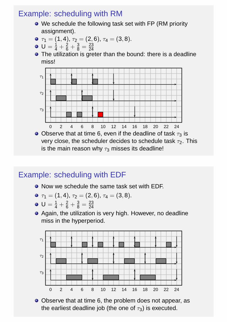
Example: scheduling with RMWe schedule the following task set with FP (RM priorityassignment).τ1 = (1, 4), τ2 = (2, 6), τ4 = (3, 8).U = 1

4 + 26 + 3

8 = 2324

The utilization is greter than the bound: there is a deadlinemiss!

0 2 4 6 8 10 12 14 16 18 20 22 24

τ1

τ2

τ3

Observe that at time 6, even if the deadline of task τ3 isvery close, the scheduler decides to schedule task τ2. Thisis the main reason why τ3 misses its deadline!

Example: scheduling with EDFNow we schedule the same task set with EDF.

τ1 = (1, 4), τ2 = (2, 6), τ4 = (3, 8).

U = 14 + 2

6 + 38 = 23

24

Again, the utilization is very high. However, no deadlinemiss in the hyperperiod.

0 2 4 6 8 10 12 14 16 18 20 22 24

τ1

τ2

τ3

Observe that at time 6, the problem does not appear, asthe earliest deadline job (the one of τ3) is executed.

Job-level fixed priority

In EDF, the priority of a job is fixed.

Therefore some author is classifies EDF as of job-levelfixed priority scheduling;

LLF is a job-level dynamic priority scheduling algorithm asthe priority of a job may vary with time;

Another job-level dynamic priority scheduler is p-fair.

A general approach to schedulability analysis

We start from a completely aperiodic model.

A system consists of a (infinite) set of jobsJ = {J1, J2, . . . , Jn, . . .}.

Jk = (ak , ck , dk )

Periodic or sporadic task sets are particular cases of thissystem

EDF optimality

Theorem (Dertouzos ’73)If a set of jobs J is schedulable by an algorithm A, then it isschedulable by EDF.

Proof.The proof uses the exchange method.

Transform the schedule σA(t) into σEDF(t), step by step;

At each step, preserve schedulability.

CorollaryEDF is an optimal algorithm for single processors.

Schedulability bound for periodic/sporadic tasks

TheoremGiven a task set of periodic or sporadic tasks, with relativedeadlines equal to periods, the task set is schedulable by EDFif and only if

U =N

∑

i=1

Ci

Ti≤ 1

CorollaryEDF is an optimal algorithm, in the sense that if a task set ifschedulable, then it is schedulable by EDF.

Proof.In fact, if U > 1 no algorithm can succesfully schedule the taskset; if U ≤ 1, then the task set is schedulable by EDF x(andmaybe by other algorithms).

Advantages of EDF over FP

EDF can schedule all task sets that can be scheduled byFP, but not vice versa.

Notice also that offsets are not relevant!

There is not need to define prioritiesRemember that in FP, in case of offsets, there is not anoptimal priority assignment that is valid for all task sets

In general, EDF has less context switchesIn the previous example, you can try to count the number ofcontext switches in the first interval of time: in particular, attime 4 there is no context switch in EDF, while there is onein FP.

Optimality of EDFWe can fully utilize the processor, less idle times.

Disadvantages of EDF over FP

EDF is not provided by any commercial RTOS, because ofsome disadvantageLess predictable

Looking back at the example, let’s compare the responsetime of task τ1: in FP is always constant and minimum; inEDF is variable.

Less controllableif we want to reduce the response time of a task, in FP isonly sufficient to give him an higher priority; in EDF wecannot do anything;We have less control over the execution

Overhead

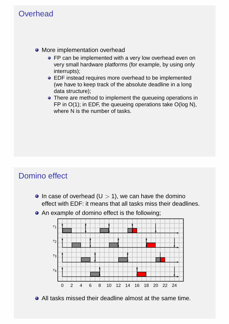
More implementation overheadFP can be implemented with a very low overhead even onvery small hardware platforms (for example, by using onlyinterrupts);EDF instead requires more overhead to be implemented(we have to keep track of the absolute deadline in a longdata structure);There are method to implement the queueing operations inFP in O(1); in EDF, the queueing operations take O(log N),where N is the number of tasks.

Domino effect

In case of overhead (U > 1), we can have the dominoeffect with EDF: it means that all tasks miss their deadlines.

An example of domino effect is the following;

0 2 4 6 8 10 12 14 16 18 20 22 24

τ1

τ2

τ3

τ4

All tasks missed their deadline almost at the same time.

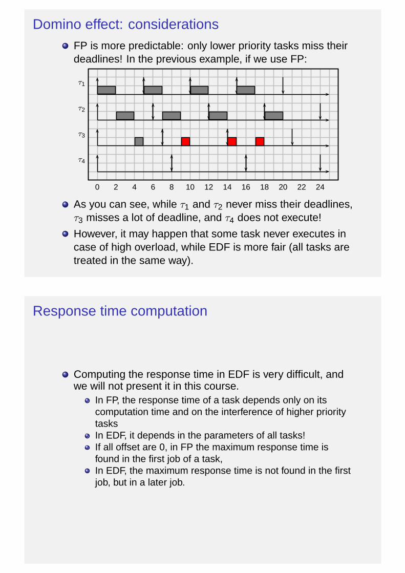
Domino effect: considerationsFP is more predictable: only lower priority tasks miss theirdeadlines! In the previous example, if we use FP:

0 2 4 6 8 10 12 14 16 18 20 22 24

τ1

τ2

τ3

τ4

As you can see, while τ1 and τ2 never miss their deadlines,τ3 misses a lot of deadline, and τ4 does not execute!

However, it may happen that some task never executes incase of high overload, while EDF is more fair (all tasks aretreated in the same way).

Response time computation

Computing the response time in EDF is very difficult, andwe will not present it in this course.

In FP, the response time of a task depends only on itscomputation time and on the interference of higher prioritytasksIn EDF, it depends in the parameters of all tasks!If all offset are 0, in FP the maximum response time isfound in the first job of a task,In EDF, the maximum response time is not found in the firstjob, but in a later job.

Generalization to deadlines different from period

EDF is still optimal when relative deadlines are not equal tothe periods

However, the schedulability analysis formula becomesmore complex

If all relative deadlines are less than or equal to theperiods, a first trivial (sufficient) test consist in substitutingTi with Di :

U ′ =N

∑

i=1

Ci

Di≤ 1

In fact, if we consider each task as a sporadic task withinterarrival time Di instead of Ti , we are increasing theutilization, U < U ′. If it is still less than 1, then the task setis schedulable. If it is larger than 1, then the task set mayor may not be schedulable

Demand bound analysis

In the following slides, we present a general methodologyfor schedulability analysis of EDF scheduling

Let’s start from the concept of demand function

Definition: the demand function for a task τi is a functionof an interval [t1, t2] that gives the amount of computationtime that must be completed in [t1, t2] for τi to beschedulable:

dfi(t1, t2) =∑

aij≥t1dij≤t2

cij

For the entire task set:

df (t1, t2) =N

∑

i=0

dfi(t1, t2)

Example of demand function

τ1 = (1, 4, 6), τ2 = (2, 6, 8), τ3 = (3, 5, 10)

0 2 4 6 8 10 12 14 16 18 20 22 24 26 28 30 32

τ1

τ2

τ3

Let’s compute df () in some intervals;

df (7, 22) = 2 · C1 + 2 · C2 + 1 · C3 = 9;

df (3, 13) = 1 · C1 = 1;

df (10, 25) = 2 · C1 + 1 · C2 + 2 · C3 = 7;

A necessary condition

TheoremA necessary condition for any job set to be schedulable by anyscheduling algorithm when executed on a single processor isthat:

∀t1, t2 df(t1, t2) ≤ t2 − t1

Proof.By contradiction. Suppose that ∃t1, t2 df(t1, t2) > t2 − t1 . If thesystem is schedulable, then it exists a scheduling algorithm thatcan execute more than t2 − t1 units of computations in aninterval of length t2 − t1. Absurd!

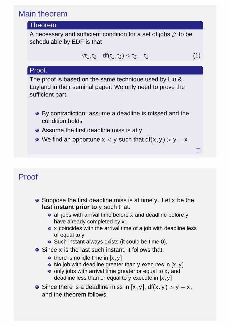
Main theoremTheoremA necessary and sufficient condition for a set of jobs J to beschedulable by EDF is that

∀t1, t2 df(t1, t2) ≤ t2 − t1 (1)

Proof.The proof is based on the same technique used by Liu &Layland in their seminal paper. We only need to prove thesufficient part.

By contradiction: assume a deadline is missed and thecondition holds

Assume the first deadline miss is at y

We find an opportune x < y such that df(x , y) > y − x .

Proof

Suppose the first deadline miss is at time y . Let x be thelast instant prior to y such that:

all jobs with arrival time before x and deadline before yhave already completed by x ;x coincides with the arrival time of a job with deadline lessof equal to ySuch instant always exists (it could be time 0).

Since x is the last such instant, it follows that:there is no idle time in [x , y ]No job with deadline greater than y executes in [x , y ]only jobs with arrival time greater or equal to x , anddeadline less than or equal to y execute in [x , y ]

Since there is a deadline miss in [x , y ], df(x , y) > y − x ,and the theorem follows.

Feasibility analysis

The previous theorem gives a first hint at how to perform aschedulability analysis.

However, the condition should be checked for all pairs[t1, t2].This is impossible in practice! (an infinite number ofintervals!).First observation: function df changes values only atdiscrete instants, corresponding to arrival times anddeadline of a job set.Second, for periodic tasks we could use some periodicity(hyperperiod) to limit the number of points to be checked toa finite set.

Simplifying the analysis

A periodic task set is synchronous if all task offsets areequal to 0

In other words, for a synchronous task set, all tasks start attime 0.

A task set is asynchronous is some task has a non-zerooffset.

Demand bound function

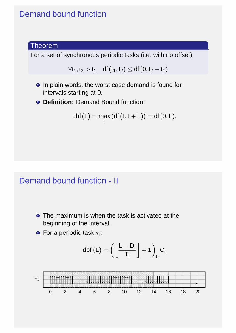
TheoremFor a set of synchronous periodic tasks (i.e. with no offset),

∀t1, t2 > t1 df (t1, t2) ≤ df (0, t2 − t1)

In plain words, the worst case demand is found forintervals starting at 0.

Definition: Demand Bound function:

dbf (L) = maxt

(df (t , t + L)) = df (0, L).

Demand bound function - II

The maximum is when the task is activated at thebeginning of the interval.

For a periodic task τi :

dbfi(L) =

(⌊

L − Di

Ti

⌋

+ 1)

0Ci

0 2 4 6 8 10 12 14 16 18 20

τ1

Synchronous periodic task sets

Theorem (Baruah, Howell, Rosier ’90)

A synchronous periodic task set T is schedulable by EDFif and only if:

∀L ∈ dead(T ) dbf(L) ≤ L

where dead(T ) is the set of deadlines in [0, H]

Proof next slide.

Proof

Sufficiency: eq. holds → task set is schedulable.By contradictionIf deadline is missed in y , then ∃x , y y − x < df(x , y)it follows that y − x < df(x , y) ≤ dbf(y − x)

Necessity: task set is schedulable → eq. holdsBy contradictioneq. does not hold for L.build a schedule starting at 0, for which dbf(L) = df(0, L)Hence task set is not schedulable

Sporadic task

Sporadic tasks are equivalent to synchronous periodic tasksets.

For them, the worst case is when they all arrive at theirmaximum frequency and starting synchronously.

Synchronous and asynchronous

Let T be a asynchronous task set.

We call T ′ the corresponding synchronous set, obtained bysetting all offset equal to 0.

Corollary

If T ′ is schedulable, then T is schedulable too.

Conversely, if T is schedulable, T ′ may not be schedulable.

The proof follows from the definition of dbf(L).

A pseudo-polynomial test

Theorem (Baruah, Howell, Rosier, ’90)Given a synchronous periodic task set T , with deadlines lessthan or equal to the period, and with load U < 1, the system isschedulable by EDF if and only if:

∀L ∈ deadShort(T ) dbf(L) ≤ L

where deadShort(T ) is the set of all deadlines in interval [0, L∗]and

L∗ =U

1 − Umax

i(Ti − Di)

CorollaryThe complexity of the above analysis is pseudo-polynomial.

Example of computation of the dbfτ1 = (1, 4, 6), τ2 = (2, 6, 8), τ3 = (3, 5, 10)

U = 1/6 + 1/4 + 3/10 = 0.7167, L∗ = 12.64.We must analyze all deadlines in [0, 12], i.e. (3, 5, 6, 10).

0 2 4 6 8 10 12 14 16 18 20 22 24 26 28 30 32

τ1

τ2

τ3

Let’s compute dbf ()df (0, 4) = C1 = 1 < 4;df (0, 5) = C1 + C3 = 4 < 5;df (0, 6) = C1 + C2 + C3 = 6 ≤ 6;df (0, 10) = 2C1 + C2 + C3 = 7 ≤ 10;The task set is schedulable.

Idle time and busy period

The interval between time 0 and the first idle time is calledbusy period.

The analysis can be stopped at the first idle time (Spuri,’94).

The first idle time can be found with the following recursiveequations:

W (0) =N

∑

i=1

Ci

W (k) =N

∑

i=1

⌈

W (k − 1)

Ti

⌉

Ci

The iteration stops when W (k − 1) = W (k).

Another example

Consider the following example

Ci Di Ti

τ1 1 2 4τ2 2 4 5τ3 4.5 8 15

U = 0.9; L∗ = 9 ∗ 7 = 63;

W = 14.5.

Then we can check all deadline in interval [0, 14.5].

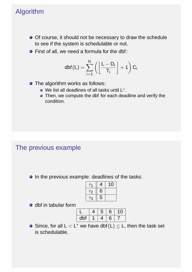
Algorithm

Of course, it should not be necessary to draw the scheduleto see if the system is schedulable or not.

First of all, we need a formula for the dbf :

dbf (L) =N

∑

i=1

(⌊

L − Di

Ti

⌋

+ 1)

Ci

The algorithm works as follows:We list all deadlines of all tasks until L∗.Then, we compute the dbf for each deadline and verify thecondition.

The previous example

In the previous example: deadlines of the tasks:

τ1 4 10τ2 6τ3 5

dbf in tabular formL 4 5 6 10dbf 1 4 6 7

Since, for all L < L∗ we have dbf (L) ≤ L, then the task setis schedulable.

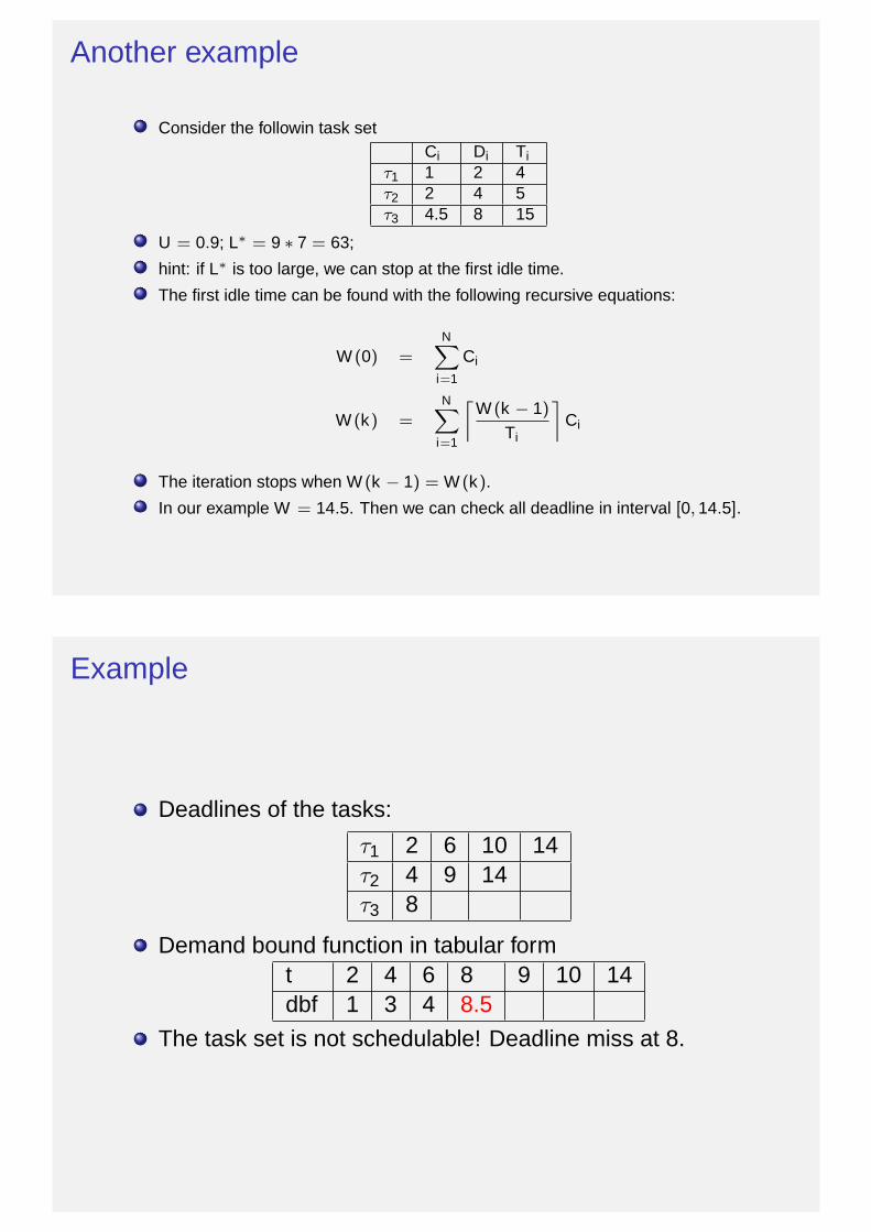
Another example

Consider the followin task setCi Di Ti

τ1 1 2 4τ2 2 4 5τ3 4.5 8 15

U = 0.9; L∗ = 9 ∗ 7 = 63;

hint: if L∗ is too large, we can stop at the first idle time.

The first idle time can be found with the following recursive equations:

W (0) =

NX

i=1

Ci

W (k) =

NX

i=1

‰

W (k − 1)

Ti

ı

Ci

The iteration stops when W (k − 1) = W (k).

In our example W = 14.5. Then we can check all deadline in interval [0, 14.5].

Example

Deadlines of the tasks:

τ1 2 6 10 14τ2 4 9 14τ3 8

Demand bound function in tabular formt 2 4 6 8 9 10 14dbf 1 3 4 8.5

The task set is not schedulable! Deadline miss at 8.

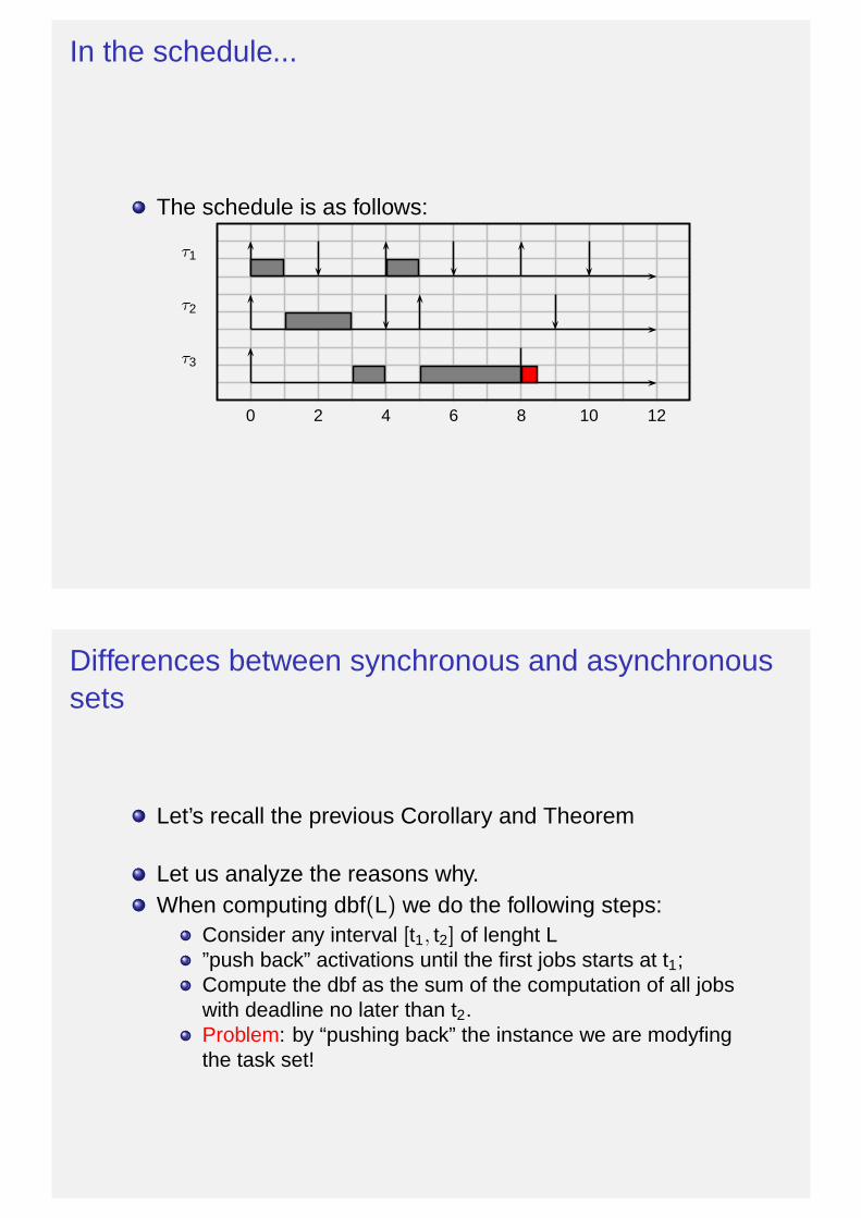
In the schedule...

The schedule is as follows:

0 2 4 6 8 10 12

τ1

τ2

τ3

Differences between synchronous and asynchronoussets

Let’s recall the previous Corollary and Theorem

Let us analyze the reasons why.When computing dbf(L) we do the following steps:

Consider any interval [t1, t2] of lenght L”push back” activations until the first jobs starts at t1;Compute the dbf as the sum of the computation of all jobswith deadline no later than t2.Problem: by “pushing back” the instance we are modyfingthe task set!

Example of asynchronous task set

τ1 = (0, 4, 7, 9) and τ2 = (2, 5, 8, 12)

0 2 4 6 8 10 12 14 16 18 20 22 24 26 28

τ1

τ2

df(0, 8) = 4

df(2, 10) = 5

Example of asynchronous task set

τ1 = (0, 4, 7, 9) and τ2 = (2, 5, 8, 12)

0 2 4 6 8 10 12 14 16 18 20 22 24 26 28

τ1

τ2

dbf(8) = 9

The dbf is too pessimistic.

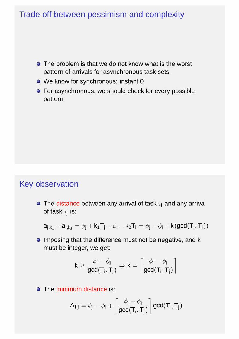
Trade off between pessimism and complexity

The problem is that we do not know what is the worstpattern of arrivals for asynchronous task sets.

We know for synchronous: instant 0

For asynchronous, we should check for every possiblepattern

Key observation

The distance between any arrival of task τi and any arrivalof task τj is:

aj,k1 − ai,k2 = φj + k1Tj −φi − k2Ti = φj −φi + k(gcd(Ti , Tj))

Imposing that the difference must not be negative, and kmust be integer, we get:

k ≥φi − φj

gcd(Ti , Tj)⇒ k =

⌈

φi − φj

gcd(Ti , Tj)

⌉

The minimum distance is:

∆i,j = φj − φi +

⌈

φi − φj

gcd(Ti , Tj)

⌉

gcd(Ti , Tj)

Observations

From the formula we can derive the following observations:

The value of ∆i,j is an integer in interval [0, gcd(Ti , Tj) − 1]If Ti and Tj are prime between them (i.e. gcd = 1), then∆i,j = 0.

Now we are ready to explain the basic idea behind the newscheduling analysis methodology.

Basic Idea

Given an hypothetical interval [x , y ]

Assume task τi arrival time coincides with xWe “push back” all other tasks until they reach theminimum distance from τi arrival time

there is no need to push it back further (it would be toopessimistic!)

The df in all intervals starting with x can only increase afterthe “pushing back”.

Therefore, if no deadline is missed in [x , y ], then nodeadline is missed in any interval of length (y − x).

We could build such interval by selecting a task τi to startat the beginning of the interval, and setting the arrivaltimes of the other tasks at their minimum distances

Problem

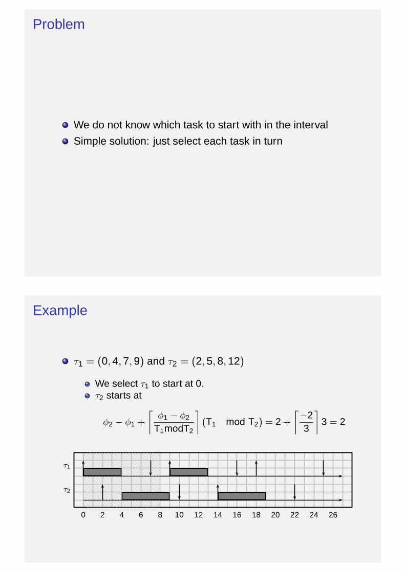
We do not know which task to start with in the interval

Simple solution: just select each task in turn

Example

τ1 = (0, 4, 7, 9) and τ2 = (2, 5, 8, 12)

We select τ1 to start at 0.τ2 starts at

φ2 − φ1 +

⌈

φ1 − φ2

T1modT2

⌉

(T1 mod T2) = 2 +

⌈

−23

⌉

3 = 2

0 2 4 6 8 10 12 14 16 18 20 22 24 26

τ1

τ2

Example

τ1 = (0, 4, 7, 9) and τ2 = (2, 5, 8, 12)

Next, we select τ2 to start at 0.

τ1 starts at

φ1 − φ2 +

⌈

φ2 − φ1

T2 mod T1

⌉

(T2 mod T1) = −2 +

⌈

23

⌉

3 = 1

0 2 4 6 8 10 12 14 16 18 20 22 24 26

τ1

τ2

Main theorem

Given an asynchronous task set TLet T ′

i be the task set obtained byfixing the offset of τi at 0setting the offset of all other tasks at their minimumdistance from τi

Theorem (Pellizzoni and Lipari, ECRTS ’04)Given task set T with U ≤ 1, scheduled on a single processor,if ∀ 1 ≤ i ≤ N all deadlines in task set T ′

i are met until the firstidle time, then T is feasible.

Performance

0.8 0.82 0.84 0.86 0.88 0.9 0.92 0.94 0.96 0.98 10.4

0.5

0.6

0.7

0.8

0.9

1

total utilization

perc

enta

ge o

f fea

sibl

e ta

sk s

ets

synchronous1 fixed task2 fixed tasks3 fixed tasksNP−Hard

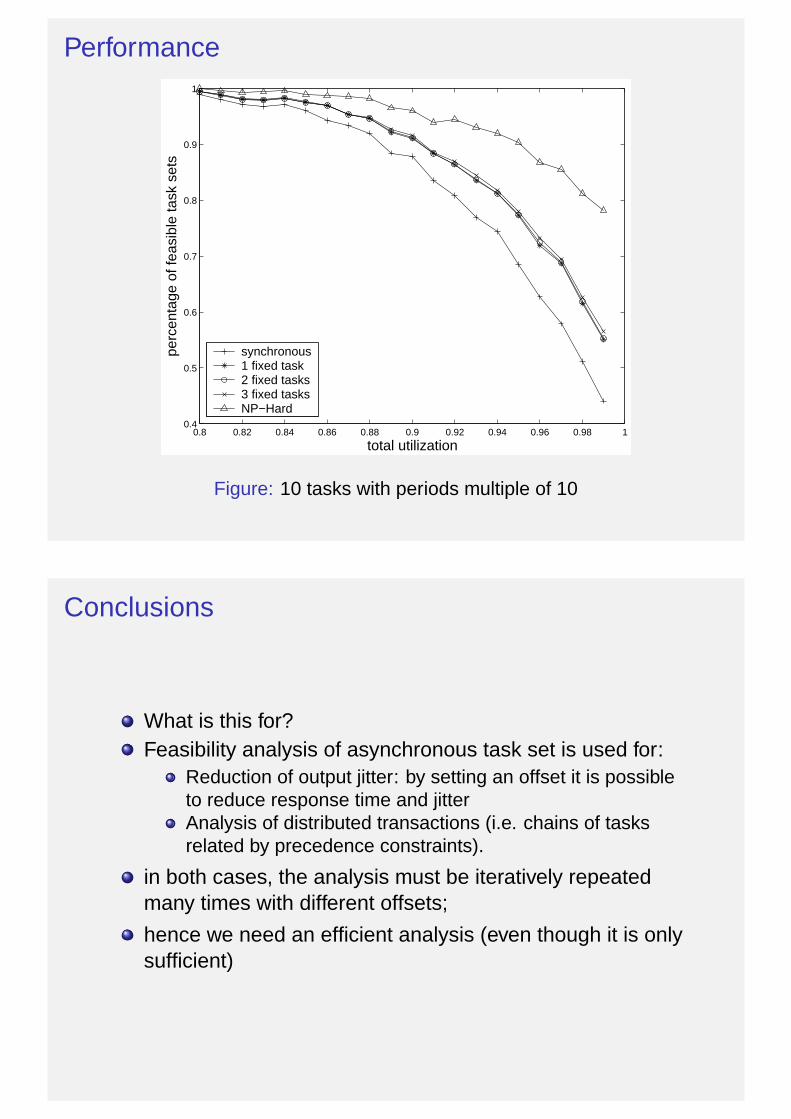
Figure: 10 tasks with periods multiple of 10

Conclusions

What is this for?Feasibility analysis of asynchronous task set is used for:

Reduction of output jitter: by setting an offset it is possibleto reduce response time and jitterAnalysis of distributed transactions (i.e. chains of tasksrelated by precedence constraints).

in both cases, the analysis must be iteratively repeatedmany times with different offsets;

hence we need an efficient analysis (even though it is onlysufficient)

References I

M. L. DertouzosControl Robotics: The Procedural Control of PhysicalProcessesInformation Processing, 1974

@ J.Y.-T. Leung and M.L. Merril,A Note on Preemptive Scheduling of Periodic Real-TimeTasksInformation Processing Letters, vol 3, no 11, 1980

S.K. Baruah, L.E. Rosier and R.R. Howell,Algorithms and Complexity Concerning the PreemptiveScheduling of Periodic Real-Time Tasks on One ProcessorReal-Time Systems Journal, vol. 2, 1990

References II

R. Pellizzoni and G. LipariFeasibility Analysis of Real-Time Periodic Tasks withOffsetsReal-Time Systems Journal, 2005