ECOTONAL CHANGE IN HIGH-ELEVATION FORESTS OF THE GREAT SMOKY

MOUNTAINS, 1930S-2004

by

JULIE PAIGE TUTTLE

(Under the Direction of ALBERT J. PARKER)

ABSTRACT

Recent theory asserts that montane vegetation ecotones may be good locations for

observing change because of their association with steep environmental and climatic gradients.

In 2004, I sampled the Great Smoky Mountains spruce-fir ecotone for comparison to Frank

Miller’s 1930s data to examine changes in ecotonal forest composition and structure. Changes in

stand attributes as well as shifts in dominant and subdominant species reflect primarily the

decimation of Abies fraseri by the balsam woolly adelgid and high mortality of Fagus

grandifolia from beech bark disease. Based on the results of this study, the abundance and

distribution of Picea rubens seem preserved in the ecotone, pending future recruitment success.

Abies fraseri persists in a diminished state at the highest elevations. It is unknown whether

Betula lutea will persist in dominating former A. fraseri forests, particularly on north-facing

slopes.

INDEX WORDS: spruce-fir, montane ecotone, Great Smoky Mountains, Picea rubens, Abies

fraseri, balsam woolly adelgid, global change, forest disturbance

ECOTONAL CHANGE IN HIGH-ELEVATION FORESTS OF THE GREAT SMOKY

MOUNTAINS, 1930S-2004

by

JULIE PAIGE TUTTLE

B.S., Southern Methodist University, Dallas, Texas, 1988

A Thesis Submitted to the Graduate Faculty of The University of Georgia in Partial Fulfillment

of the Requirements for the Degree

MASTER OF SCIENCE

ATHENS, GEORGIA

2007

© 2007

Julie Paige Tuttle

All Rights Reserved

ECOTONAL CHANGE IN HIGH-ELEVATION FORESTS OF THE GREAT SMOKY

MOUNTAINS, 1930S-2004

by

JULIE PAIGE TUTTLE

Major Professor: Albert J. Parker

Committee: Kathleen C. Parker Marguerite Madden

Electronic Version Approved: Maureen Grasso Dean of the Graduate School The University of Georgia May 2007

DEDICATION

To Carolyn and Sam Donald

iv

ACKNOWLEDGEMENTS

The most important thanks go to my father, Bill Tuttle, without whose heroic willingness

to help in the field this project would have flopped. His quick comprehension and sharp

attention to detail were ideal. While my father and I were in the field, my mother braved a

hurricane, safely evacuating herself and my cat, Monster. My grandparents, Sam and Carolyn

Donald, have been unfailing pillars of support and encouragement as I find my way in this world.

I extend my profound gratitude to my advisor, Al Parker, for his patience, resilience,

insight, encouragement, ideas, feedback, and perhaps most important, his compassion. Thanks to

my entire committee, past and present – Al Parker, Kathy Parker, Elgene Box, and Marguerite

Madden – all top-notch scientists with high ethical standards, whose input set the stage for

developing my research interests and this project.

Thanks to Joshua Kincaid for the tip that led to this project. I am indebted to those who

provided data: Marguerite and the UGA Center for Remote Sensing and Mapping Science (and

the National Park Service for permission), for their vegetation classification of Great Smoky

Mountains National Park and other GIS layers, as well as Peter White and the University of

North Carolina’s Plant Ecology Lab for the digitized Miller data, the Miller topographic maps,

and additional GIS layers. Thanks to the scientists and staff of Great Smoky Mountains National

Park for permission to conduct research in the park and logistical assistance during the project.

Several talented, diverse, and indispensable field assistants made this project a success:

Bill Tuttle, Bernard Patten, Mark Lawrence, Louis Manglass, Stuart Whipple, Seth Bata,

Michelle Luebke, Joel Sabin, Joshua Kincaid, Vanese Flood, and Ron White. Steve Walsh, my

v

Ph.D. advisor at the University of North Carolina, provided needed structure here in North

Carolina in the final weeks of writing. Finally, I give special thanks to Peter White of the

University of North Carolina for extremely helpful conversations, input, and encouragement; his

generous assistance in organizing my results propelled the thesis toward completion.

vi

TABLE OF CONTENTS

Page

ACKNOWLEDGEMENTS.............................................................................................................v

LIST OF TABLES......................................................................................................................... ix

LIST OF FIGURES .........................................................................................................................x

CHAPTER

1 Introduction....................................................................................................................1

2 Study Area .....................................................................................................................5

3 Methods..........................................................................................................................7

Miller data .................................................................................................................7

Field data collection ..................................................................................................8

Data preparation ......................................................................................................10

Analysis ...................................................................................................................11

4 Results..........................................................................................................................15

Stand summary, species composition, and structure ...............................................15

Stand summary and species composition by elevation ...........................................22

Community types ....................................................................................................30

Community gradients ..............................................................................................31

Species-topography relationships............................................................................40

5 Discussion....................................................................................................................49

Ecotonal change ......................................................................................................49

vii

Related findings.......................................................................................................52

Summary of impacts and consideration of future dynamics ...................................56

REFERENCES ..............................................................................................................................60

viii

LIST OF TABLES

Page

Table 1: Range of topographic and environmental setting for the Miller and Tuttle samples ......17

Table 2: Summary of stand basal area, density, and diversity for the Miller and Tuttle data .......19

Table 3: Mean plot species abundances and frequency of occurrence for the Miller

and Tuttle data ...............................................................................................................20

Table 4: Pearson correlations of species basal with ordination axes for nonmetric

multidimensional scaling (NMS) of the combined Miller and Tuttle data ...................33

Table 5: Pearson correlations of species basal area with ordination axes for the Miller NMS .....38

Table 6: Pearson correlations of species basal area with ordination axes for the Tuttle NMS......39

Table 7: Canonical correspondence analysis (CCA) results for the Miller and Tuttle data ..........42

ix

LIST OF FIGURES

Page

Figure 1: Study area: the spruce-fir zone and its ecotone with northern hardwood forests

in Great Smoky Mountains National Park ......................................................................6

Figure 2: Location of Miller comparison plots (1930s) and Tuttle plots (2004) in the study

area of Great Smoky Mountains National Park.............................................................16

Figure 3: Size-class distributions for the Miller and Tuttle data based on total plot density ........20

Figure 4: Size-class distributions for species with the highest densities in the Miller

or Tuttle data .................................................................................................................22

Figure 5: Size-class distributions for other important species in the Miller and Tuttle data .........23

Figure 6: Mean plot basal area and density by elevation zone for the Miller and Tuttle data.......24

Figure 7: Mean species basal area by elevation zone for the Miller and Tuttle data.....................26

Figure 8: Mean species density by elevation zone for the Miller and Tuttle data .........................27

Figure 9: Mean species importance value by elevation zone for the Miller and Tuttle data.........28

Figure 10: Nonmetric multidimensional scaling (NMS) of the Miller and Tuttle plots

combined as one data set ...............................................................................................31

Figure 11: NMS of the combined Miller and Tuttle plots, with cluster types from the

combined Miller-Tuttle cluster analysis........................................................................34

Figure 12: NMS of the Miller data, with cluster types ..................................................................35

Figure 13: NMS of the Tuttle data, with cluster types...................................................................36

Figure 14: NMS of the combined Miller and Tuttle plots, with cluster types from the

x

separate Miller and Tuttle cluster analyses ...................................................................40

Figure 15: Canonical correspondence analysis (CCA) biplot for the Miller data, axes 1 and 3 ...43

Figure 16: Canonical correspondence analysis (CCA) biplot for the Miller data, axes 2 and 3 ...44

Figure 17: Canonical correspondence analysis (CCA) biplot for the Tuttle data, axes 1 and 3....45

Figure 18: Canonical correspondence analysis (CCA) biplot for the Tuttle data, axes 2 and 3....46

xi

Chapter 1: Introduction

Great Smoky Mountains National Park (GRSM) is prized for its biodiversity and represents

one of the largest expanses of protected forest in the eastern United States (211,041 ha). While

creation of the park in 1934 ended human settlement, livestock grazing, logging, and post-

logging fires within park boundaries, other anthropogenic impacts transgress geographic

boundaries and continue to impose change on the forests of the Great Smoky Mountains. Recent

and potential future threats to GRSM forests include exotic pest introduction, atmospheric

deposition, altered disturbance regimes, and climate change, all of which affect forest

composition and structure.

In particular, GRSM’s high-elevation spruce-fir forests, thought to be glacial relicts (White

and Cogbill 1992), have been exposed to multiple anthropogenic stressors, including extensive

pre-park logging of red spruce (Picea rubens) (Pyle 1988), decimation of Fraser fir (Abies

fraseri) by the non-native balsam woolly adelgid (Adelges piceae Ratz.) (Smith and Nicholas

1998), and increased stress on P. rubens from atmospheric deposition associated with

anthropogenic atmospheric inputs (McLaughlin et al. 1993), such as nitric oxides, sulfur dioxide,

and ozone. These high-elevation forests contribute to the biodiversity of GRSM; for example, A.

fraseri is endemic to the southern Appalachian Mountains, and spruce-fir forests provide habitat

for species such as the endangered spruce-fir moss spider (Microhexura montivaga) (Keith

Langdon, personal communication 2004). Consequently, ecological monitoring and analysis of

GRSM and other southern Appalachian spruce-fir forests have been ongoing for several decades.

1 1

While the study of spruce-fir forests has yielded valuable insight into their response to the

range of anthropogenic inputs, most studies have been focused within areas dominated by P.

rubens and A. fraseri (White and Busing 1993). Recent theory, however, asserts that vegetation

ecotones, the transition zone between different vegetation types, may be important indicators of

change, because species are at their environmental or competitive limits (Gosz 1992, Noble

1993) at these locations. Montane vegetation ecotones in particular, because of their association

with steep environmental and climatic gradients, may be good locations for observing change

(Beniston 1994). Indeed, paleoecological studies suggest that migration of montane ecotones

occurs with changes such as climate warming or altered disturbance regimes (Delcourt and

Delcourt 1998). Ecotonal change at observable human time scales may not manifest as a clear

shift in vegetation boundaries, especially where vegetation transitions are not abrupt; rather,

compositional shifts within or on either side of an ecotone may be the most evident change

(Payette et al. 2001). Regardless, ecotonal studies over recent decades have contributed to an

understanding of forest dynamics and change.

The lower boundary of GRSM spruce-fir forests represents both a montane deciduous-

coniferous ecotone and the lower latitudinal extent of postglacial remnant “boreal” forest in

eastern North America (White and Cogbill 1992), making its dynamics of interest in the study of

anthropogenic forest change. In addition, rapid regeneration of A. fraseri after balsam woolly

adelgid infestation (Busing et al. 1988, personal observation 2004) and lower mortality of

southern, as compared with northern, P. rubens populations from atmospheric deposition (Peart

et al. 1992) may combine with other factors (e.g., long lifespan or adaptation to site exposure) to

enable persistence of high-elevation P. rubens- and A. fraseri-dominated forests in spite of such

impacts, perhaps supporting the relevance of investigating the deciduous-coniferous ecotone as a

2 2

more sensitive indicator of change. Few studies exist, however, focused on montane deciduous-

coniferous ecotones in general (Kupfer and Cairns 1996) and the GRSM deciduous-coniferous

ecotone in particular (White and Busing 1993).

While multiple field vegetation surveys have been conducted in GRSM – most notably those

by Cain (1935), Oosting and Billings (1951), Whittaker (1956), and Golden (1981) – the most

comprehensive field survey of GRSM vegetation was conducted by Frank Miller in 1935-1938

(MacKenzie and White 1998). Miller’s inclusion of over 133 plots spanning the spruce-fir zone

and its ecotone with lower-elevation, primarily northern hardwood forests (Busing et al. 1993)

offers an opportunity for analysis of ecotonal change over several decades. Busing et al. (1993)

analyzed the Miller ecotonal data, but such a comparison with the present-day ecotone has not

been conducted. In 2004, therefore, I sampled the GRSM deciduous-coniferous ecotone for

comparison to the Miller data to examine changes in ecotonal forest composition and structure

over nearly 70 years.

It should be noted that several factors complicate any study of ecotones and of montane

ecotones in particular. The universal value of vegetation ecotones as indicators of both natural

and anthropogenic change remains indeterminate; results of studies and models have been site,

situation, and time specific. Some studies reveal rapid shifts or changes in ecotones (Allen and

Breshears 1998) and others remain inconclusive (Masek 2001). Similar biome transitions in

different geographic contexts may exhibit directionally opposite shifts in response to similar

inputs, such as fire suppression (Grau and Veblen 2000). Time lags related to such factors as the

persistence of established, long-lived trees (e.g., P. rubens) and vegetation-reinforced soil

gradients (e.g., acidity) may prevent compositional change in temporal step with inputs (White

and Cogbill 1992, Malanson 1999). Several factors make causal attribution and modeling or

3 3

prediction of ecotonal change difficult: multiple interactive causes of change across spatial and

temporal scales (Hofgaard 1997); feedbacks that enhance or mitigate vegetation responses

(Malanson 1999); and individualistic species behavior (White and Cogbill 1992, Woodward

1993). The study of montane ecotones is complicated further by the influence of complex

topographic gradients, including slope aspect, steepness, configuration, and position, on

vegetation composition (Parker 1982, Welch et al. 2002).

The above challenges notwithstanding, this study has two objectives: 1) detection of change

(or lack of change) in the deciduous-coniferous ecotone of GRSM and 2) examination of

composition-topography relationships within this montane ecotone. To this end, I address the

following questions: 1) Have forest stand attributes (basal area, density, and diversity) or species

composition and abundance in the ecotone changed since the 1930s? 2) Has stand or species

size-class structure changed?) 3) Have stand attributes or species composition and abundance

changed by elevation within the ecotone? 4) Have ecotone community types and gradients

changed? 5) Have compositional relationships to topographic variables changed for the ecotone?

4 4

5

Chapter 2: Study Area

Great Smoky Mountains National Park (35˚ 41’ N, 83˚ 32’ W) contains the largest remaining

tract of undisturbed spruce-fir forest in the southern Appalachians (48% of original area),

occurring from approximately 1500 m up to 2025 m at Clingmans Dome (White and Cogbill

1992) and surrounded mostly by northern hardwood forest at its lower boundary (Figure 1). This

lower boundary has been related to a mean July temperature of 17˚ C; a hypothesized

relationship with frequency of cloud immersion; and increased precipitation with elevation,

ranging from 180 to 250 cm per year in the southern Appalachian spruce-fir zone (White and

Cogbill 1992). The dominants of southern Appalachian spruce-fir forests, red spruce (Picea

rubens) and Fraser fir (Abies fraseri), exhibit individualistic behavior, however. While A. fraseri

rarely occurs below 1372 m in the southern Appalachians (Burns and Honkala 1990), P. rubens

may occur with hardwoods and Eastern hemlock (Tsuga canadensis) as low as, and perhaps

below, 1200 m in GRSM according to a recent remote sensing-based classification (Madden et

al. 2004), although the accuracy assessment of this classification has not yet been completed.

However, as a result of the frequent occurrence of P. rubens at lower elevations than A. fraseri,

the deciduous-coniferous ecotone in GRSM largely involves P. rubens.

Bedrock in GRSM comprises primarily the Thunderhead and Anakeesta formations,

metamorphosed sedimentary rock of the late Precambrian era (Moore 1988). Soils of the spruce-

fir zone are shallow, acidic Inceptisols or Spodosols (Burns and Honkala 1990). With decreasing

elevation and slope steepness, soils generally become deeper and less acidic (Fernandez 1992).

5

6

Figure 1. Study area: the spruce-fir zone and its ecotone with northern hardwood forests in Great Smoky Mountains National Park. The map was created in ESRI ArcMap 8.1 using the CRMS vegetation classification data (Madden et al. 2004), a USGS 30-m DEM, and the National Park Service’s GRSM boundary shapefile.

±

northern hardwood - no spruce or fir nondominant spruce or firdominant spruce-fir

0 10 205Kilometers

NC

southeastern U.S.

TN

6

Chapter 3: Methods

Busing et al. (1993) identified 133 undisturbed Miller plots in 13 watersheds containing any

Picea rubens or Abies fraseri >4 in. diameter at breast height (dbh). Results of their analysis

suggest a topographically complex, gradual ecotone from primarily northern hardwood to

spruce-fir forest between 1300 and 1600 m elevation. My approach in this study is therefore to

assess change in forest composition and structure within this gradual ecotone, across the range of

topographic settings present. Uncertainty in the Miller plot locations makes relocation for direct

resampling difficult and the results of any subsequent paired analysis questionable; consequently,

I collected an independent sample of ecotone plots for comparison to a topographically similar

subset of Miller ecotone plots.

Botanical nomenclature follows Weakley (2007).

Miller data. The Miller field crews sampled park vegetation in a fairly regular grid of 1 x 2-

chain (20 x 40-m) plots across the entire park, with only a few areas sparsely sampled. In each

plot, all trees >4 in. (10.1 cm) dbh were identified to species and tallied in four diameter classes:

4-<12 in. (10.1-30.3 cm), 12-<24 in. (30.4-60.8 cm), 24-<36 in. (60.9-90.3 cm), and ≥36 in.

(>90.3 cm). Environmental data recorded for each plot include elevation (ft), slope steepness

(%), slope aspect (SW, S, W, SE, NW, E, N, and NE), soil depth and texture, litter depth, and

year of most recent logging or fire. The dominant species in the shrub/sapling layer was

recorded for each of 100 contiguous, 2 x 2-m subsections within a ½ x 2-chain (10 x 40-m)

subplot. Each plot location was marked with an X and an alphanumeric label on early

topographic maps. The Uplands Field Research Laboratory (UFRL) of GRSM created digital

7 7

files of the Miller vegetation and environmental data from the original data sheets and transferred

the plot X locations to modern 1:24,000 scale USGS topographic quadrangle maps, based on the

early maps and descriptions of plot location on the data sheets (Busing et al. 1993). Both

inaccuracies in the early topographic maps and the lack of modern GPS technology contribute to

locational uncertainty for the Miller plots; plot locations as transferred to the modern topographic

maps are thought to be accurate to within approximately 50 m (Peter White, personal

communication 2004).

Field data collection. Field sampling was designed 1) to represent the geographic extent of

the spruce-fir zone in the park, 2) to “bracket” the presumed 1300-1600-m altitudinal range of

the northern hardwood and spruce-fir ecotone, and 3) to encompass the range of site types. Five

watersheds spanning the spruce-fir zone were selected to maximize the number of undisturbed

Miller ecotone plots for comparison, the overall quantity of remaining old-growth forest, and site

accessibility. Busing et al. (1993) tallied by watershed the number of undisturbed Miller ecotone

plots, and Pyle (1988) compiled historical data to estimate the percentage of remaining old-

growth forest in each watershed. Preliminary site accessibility was evaluated considering

location of roads and trails on the GRSM park map, inspection of elevation and terrain on USGS

topographic quadrangle maps, and insights from field reconnaissance. Field sampling included

sites between 1200 and 1700 m, stratified in each watershed by five 100-m elevation zones and

eight aspect classes.

Accessible sites were defined and located more specifically during the site selection process.

Preliminary site selection was accomplished by geographic information systems (GIS) analysis

using 1) a digital map of GRSM vegetation, based on manual interpretation of 1997-98 1:12,000-

scale color infrared aerial photography and recently completed by the University of Georgia’s

8 8

Center for Remote Sensing and Mapping Science (CRMS) as part of a cooperative agreement

with the National Park Service (NPS) (Madden et al. 2004); 2) a USGS 10-m digital elevation

model (DEM) of the park, provided by the Plant Ecology Lab at the University of North

Carolina; and 3) USGS digital line graph (DLG) roads, trails, and watersheds for GRSM,

provided by the park via CRMS. The sampling universe was created by selecting all vegetation

between 1200 and 1700 m that was classified by CRMS as dominated or codominated by

northern hardwoods/Tsuga canadensis, Picea rubens, or P. rubens-Abies fraseri. Slope

steepness and aspect were calculated from the DEM. To accommodate time and labor

constraints, sites within 150 m of a trail or road and with slope steepness less than or equal to

60% were selected from this sampling universe. Field reconnaissance also revealed that

reasonable access to many sites was obstructed by a dense understory of Rhododendron species,

so sites mapped by CRMS as dominated or codominated by Rhododendron spp. or Kalmia sp.

were excluded. The resultant map of accessible sites was classified by elevation and aspect, and

random locations satisfying the stratification scheme were extracted. Final site selection in the

field was modified from these locations according to actual accessibility, topographic

homogeneity for a plot size of at least 30 x 60 m, and freedom from recent gross disturbance.

Thirty-four sites were sampled.

At each site, stratified systematic unaligned sampling was used to establish eight non-

overlapping, circular 100-m2 subplots within a 30 x 60-m rectangular plot, pooled to yield a total

area sampled of 800 m2 per plot, equal to Miller plot area. In each subplot, species and dbh (1.4

m) were recorded for all trees ≥10 cm in diameter. Saplings were tallied by species in small (>0

and <5 cm) and large (≥5 and <10 cm) diameter classes within eight nested, circular 50-m2

subplots. At each plot center, elevation (m), slope steepness (%), slope aspect (°), relative slope

9 9

position (lower, middle, or upper), cross-slope and down-slope configuration (concave, convex,

or straight), and GPS coordinates (UTM 17N, NAD27) were recorded. Qualitative site

information was noted, such as presence of common understory shrub and herbaceous species,

evidence of disturbance, abundance of downed logs, and obvious tree damage by disease or

insects.

Data preparation. Data preparation included GIS selection in ArcMap 8.1 (Environmental

Systems Research Institute, Inc.) of an appropriate subset of Miller plots for comparison to the

Tuttle field sample as well as conversion of vegetation and environmental variables in the two

data sets to comparable units or classes. The locations of all Miller plots within the five sampled

watersheds were manually digitized in UTM/NAD27 coordinates from their locations on the

modern topographic quadrangle maps. Plot environmental data were appended to the

coordinates. Using ArcMap,, the Miller plot locations were overlaid on USGS digital raster

graphics (DRGs) of the 1:24000 scale USGS topographic quadrangle maps, and DEM-derived

elevation, aspect, and slope were appended to the plot data to confirm the relative accuracy of the

digitized plot locations. Undisturbed Miller plots (no recorded date of logging or burning) that

fell within my vegetation sampling universe were selected. Because of the inherent locational

uncertainty in plot locations, Miller’s elevation, aspect, and slope values – not the DEM-derived

values – were used for the Miller data in all subsequent analyses. Thirty-two plots matching the

Tuttle elevation-aspect class combinations and with less than 50% cover by Rhododendron or

Kalmia spp. were identified and selected to represent the comparison data set.

MacKenzie and White (1998) calculated Miller plot basal area (m2/ha) and density (stems/ha)

by species, and Busing et al. (1993) coded aspect classes from high to low relative solar radiation

load (SW=1, S=2, W=3, SE=4, NW=5, E=6, N=7, and NE=8). Basal area was calculated by

10 10

MacKenzie and White (1998) as the number of stems times basal area for the geometric mean of

each size class, summed across all four size classes and converted to meters squared per hectare.

For the Tuttle data, each plot’s basal area and density by species were calculated from the actual

measured values. Miller elevations were converted from feet to meters, and Tuttle aspect values

were coded to match Busing et al.’s (1993) classes. In preparation for size-class analysis, trees

in the Tuttle data were tallied by species in the same diameter classes as the Miller data.

Relative importance value (IV), defined as the sum of relative basal area and relative density,

was calculated by species for each Miller and Tuttle plot. The topographic convergence index

(TCI), calculated for GRSM and provided by Jobe (2006), was extracted by GIS for all plot

locations and was included with elevation, aspect, and slope steepness as a topographic variable

in all subsequent analyses. TCI represents the impact of relative slope position and configuration

on site potential moisture availability, as a function of upslope drainage area (a) and local slope

steepness (tanß) (TCI = ln(a/tanß)) (Beven and Kirkby 1979). Along with elevation, aspect,

and slope steepness, TCI has been related to vegetation composition gradients (Urban 2000).

Analysis. Basal area and stem density were summarized for each data set by plot and by

species. Importance value (IV) and frequency of occurrence (%) additionally were summarized

by species. Species richness, species evenness, and Shannon’s diversity index were computed

for each plot. Differences in stand attributes were assessed using Student’s t-test to compare

Miller and Tuttle mean plot basal area, density, species richness, species evenness, and

Shannon’s diversity index. Benjamini and Hochberg’s method was used to control the false

discovery rate, or the expected proportion of rejected null hypotheses that are erroneously

rejected in the setting of multiple significance tests (Benjamini and Hochberg 1995). Differences

in species composition and abundance between the two data sets were assessed by visual

11 11

comparison of species’ mean basal area, density, IV, and frequency of occurrence. Graphs of

mean stem density by size class for Miller versus Tuttle stands and species were compared to

ascertain differences in size-class structure. To examine stand differences within the ecotone,

mean plot basal area and stem density by elevation zone were calculated and compared.

Likewise, mean plot basal area, density, and IV were calculated for each species by elevation

zone, enabling assessment of 1) how dominant species differ by elevation between the two data

sets, 2) which species drive overall stand differences by elevation, and 3) trends in species

dominance with elevation, particularly from northern hardwood species to Picea rubens and/or

Abies fraseri.

Plots were grouped into community types for each data set separately with hierarchical,

agglomerative cluster analysis of composition by basal area using Ward’s linkage method and

relative Euclidean distance as the measure of (dis)similarity between plots. Cluster analysis also

was performed on the combined Miller and Tuttle data to evaluate overlap or separation of

community types in the two data sets. After testing several linkage methods and distance

measures, the combination of Ward’s method and relative Euclidean distance was chosen

because it yielded minimal chaining and ecologically interpretable clusters that were useful for

visual interpretation of subsequent analyses. Ward’s method, which minimizes the total error

sum of squares based on Euclidean distance of plots from cluster centroids (Ward 1963),

generally performs well with ecological data (Kent and Coker 1992), and relative Euclidean

distance relativizes abundance within plots, minimizing differences based solely on plot total

basal area. It should be noted that Sorensen distance, a commonly used distance measure that

also performs well with ecological community data (Faith et al. 1987), was not used because it is

incompatible with Ward’s method (McCune and Mefford 1999). For each of the three cluster

12 12

analyses, the final number of clusters was selected to minimize the objective function while

maximizing ecological interpretability in the context of this study.

Patterns of species composition were educed using nonmetric multidimensional scaling (NMS)

(Kruskal 1964), a distance-based ordination method for indirect gradient analysis. The

advantages and disadvantages of NMS versus detrended correspondence analysis (DCA), an

eigenanalysis-based ordination method, continue to be debated in the community ecology

literature (Faith et al. 1987, Holland and Patzkowsky 2006). After using both methods with the

Miller and Tuttle data, I chose NMS using raw basal area for ease of interpretability. Unlike the

eigenanalysis-based methods, the number of axes for NMS is user defined, and the axes are not

necessarily in order of variance explained. The best solution should minimize “stress”, the

residual sum of squares between dissimilarity in the original data matrix and distance in

ordination space, for a given number of axes and should be stable within the final iterations

(standard deviation in stress <0.00001) (McCune and Mefford 1999). I used PC-ORD for

Windows 4.37 (McCune and Mefford 1999) in autopilot mode to find the dimensionality with

the best solution and to run Monte Carlo randomization tests of significance for stress in the final

solution. Using the Sorensen distance measure (McCune and Mefford 1999), NMS ordination of

the combined Miller and Tuttle data sets was performed to compare the range of variability

present in the data sets and to visualize differences between Miller and Tuttle clusters in

ordination space. A separate NMS then was performed for each of the two data sets to assess

their community gradients independently. Correlations were performed between topographic

variables and NMS axis scores as well as between species abundances and axis scores.

To evaluate and compare compositional and species relationships to topography more directly,

canonical correspondence analysis (CCA) (ter Braak 1987) was performed on each data set

13 13

separately. CCA is considered direct gradient analysis because the ordination is constrained to a

linear regression of environmental variables on plot species composition. The user must choose

environmental variables with hypothesized relationships to composition; I used four topographic

variables – elevation, slope aspect, slope steepness, and TCI – as proxies for temperature,

precipitation, potential solar radiation, potential heat load, local site drainage, topographic

position, and site potential moisture availability. Monte Carlo tests of significance were

performed for the species-environment correlation and eigenvalue of the first ordination axis.

14 14

15

Chapter 4: Results

Thirty-two unlogged Miller plots met the elevation, aspect, and rhododendron understory

criteria to match the 34 Tuttle plots in the five study area watersheds (Figure 2). The plots

generally cover the same range of topographic and environmental setting (Table 1). The Tuttle

plots range slightly lower in elevation. Because no west-facing plots are included in the Tuttle

plots, these are also excluded from the Miller plots. The Miller plots include some steeper slopes

than the Tuttle plots. The Tuttle plots encompass a slightly wider range of topographic

convergence index (TCI) values than the Miller plots.

When plot locations are overlaid on the park’s logging history map (Pyle 1984, Kunze 2003),

one Miller plot and six Tuttle plots are located in areas mapped as heavily logged prior to park

formation (i.e., in the 1920s). However, this map is an approximation constructed from multiple

historical data types, including primarily the Miller data (the locations of which are also

approximate). Miller’s field crews recorded last year of logging, and the Miller plot location

mapped as heavily logged was recorded as unlogged. The species composition and total basal

area of this plot indicate that if logged, it was several decades earlier or not at all. If the six

Tuttle plot locations were indeed heavily logged, the stands in these locations were

approximately 70 years old by 2004. All other Miller and Tuttle plots are located in areas

mapped as selectively cut or unlogged.

Stand summary, species composition, and structure. Mean plot basal area is similar for the

Miller and Tuttle data (43.56 and 42.13 m2/ha, respectively), but mean plot density is higher for

15

16

Figure 2. Location of Miller comparison plots (1930s) and Tuttle plots (2004) in the study area of Great Smoky Mountains National Park.

±

Miller Comparison PlotsTuttle Plots

0 8 164Kilometers

16

Table 1. Range of topographic and environmental setting for the Miller and Tuttle samples. *See Results section for explanation. Miller Tuttle No. plots 32 34 No. plots with history of low to no disturbance* 31 28 Elevation (m) 1240-1707 1203-1706 Slope steepness (%) 18-125 17-72 Slope aspect classes* 1-2, 4-8 1-2, 4-8 TCI 4.02-7.33 3.47-9.52

17 17

the Tuttle data (538.6 vs. 409.7 stems/ha, p=0.015, corrected α=0.02) (Table 2). Mean plot

species richness is also higher for the Tuttle plots (p=0.0011, corrected α=0.01), while evenness

is lower, but this difference is not statistically significant (p=0.0427, corrected α=0.03).

Shannon’s diversity index is similar for the two data sets.

Total number of species recorded is 20 for the Miller data and 21 for the Tuttle data (Table 2).

Betula alleghaniensis, Picea rubens, and Fagus grandifolia are the most widespread species in

the Miller data (75, 72, and 68% of plots, respectively) and the dominant species by IV (33, 50,

and 38, respectively) (Table 3). For the Tuttle data, B. alleghaniensis and P. rubens are the most

widespread (88 and 82% of plots, respectively) and dominant (46 and 62, respectively) species.

Subdominant species in the Miller data include Abies fraseri, Tsuga canadensis, Aesculus flava,

and Acer saccharum, while T. canadensis, Halesia tetraptera var. monticola, and F. grandifolia

are subdominants in the Tuttle data.

Differences in several species’ mean basal area and density contribute to these shifts in

overstory dominance as well as understory composition (Table 3). Mean density for both P.

rubens and B. alleghaniensis in the Tuttle data is approximately twice the density for the Miller

data, while F. grandifolia basal area and density in the Tuttle data are less than half those in the

Miller data. Abies fraseri basal area is reduced by 85% and density by greater than 50% in the

Tuttle data. Tsuga canadensis density in the Tuttle data is double that of the Miller data, and H.

tetraptera basal area and density are several times greater in the Tuttle data. Aesculus flava basal

area is much lower in the Tuttle data. Distribution and abundance of several Acer species,

including A. pensylvanicum, A. spicatum, and A. rubrum, are much higher in the Tuttle data.

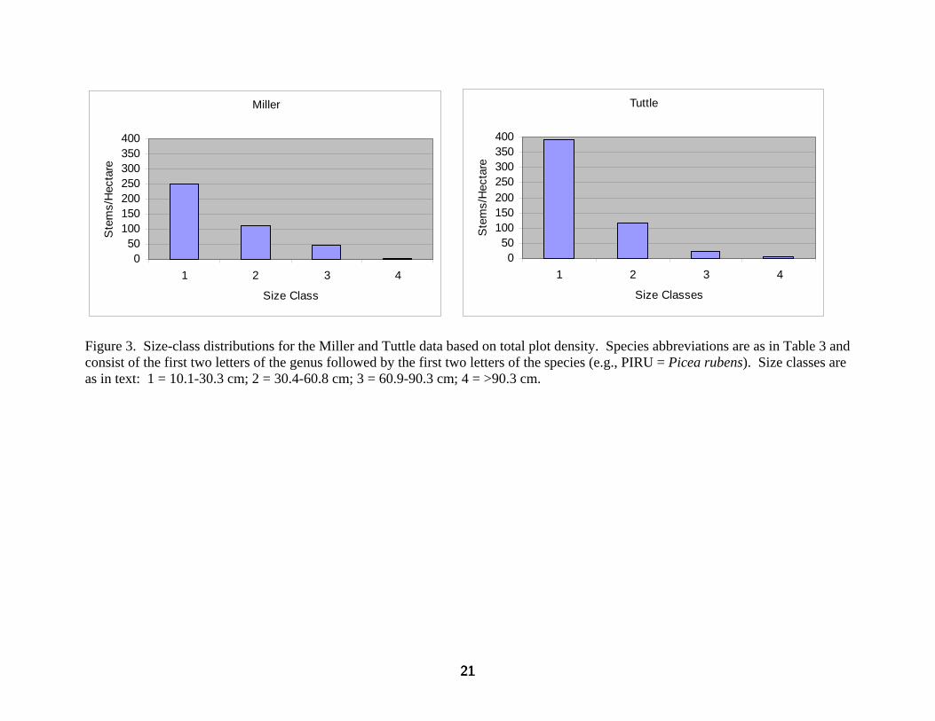
Comparison of Tuttle to Miller overall size-class distributions reveals a 57% increase in stem

density in the smallest size class with a 50% reduction in stem density for size class 3 (Figure 3).

18 18

19

Table 2. Summary of stand basal area, density, and diversity for the Miller and Tuttle data. Tuttle values significantly different from Miller values are noted: * p<0.02, ** p<0.01.

No. species recorded

Mean plot basal area (m2/ha)

Mean plot density (stems/ha)

Mean species richness

Mean species evenness

Mean Shannon's Diversity Index

Miller 20 43.56 409.70 4.80 0.74 1.13 Tuttle 21 42.13 538.60* 6.20** 0.66 1.18

19

Table 3. Mean plot species abundances and frequency of occurrence for the Miller and Tuttle data. MILLER TUTTLE

Species

Freq. (%

plots) Basal area

(m2/ha) Density

(stems/ha) Importance

Value

Freq. (%

plots) Basal area

(m2/ha) Density

(stems/ha) Importance

Value Mean SD Mean SD Mean SD Mean SD Mean SD Mean SD Abies fraseri (ABFR) 28.13 2.40 4.95 54.66 110.60 14.19 26.69 17.65 0.35 1.60 23.53 101.40 3.59 14.27 Acer pensylvanicum (ACPE) 9.38 0.03 0.08 1.13 3.55 0.58 2.22 55.88 0.44 0.59 20.22 27.01 5.66 7.11 Acer rubrum (ACRU) 3.13 0.16 0.92 1.16 6.54 0.85 4.80 26.47 1.42 3.59 13.24 31.82 6.07 14.59 Acer saccharum (ACSA) 43.75 2.75 3.93 12.91 18.58 11.39 15.89 38.24 1.52 3.40 18.01 36.57 8.17 15.45 Acer spicatum (ACSP) 3.13 0.01 0.05 0.38 2.12 0.37 2.07 23.53 0.22 0.66 9.56 22.42 2.18 5.16 Aesculus flava (AEFL) 28.13 3.65 9.10 5.31 11.98 12.31 28.53 35.30 1.29 2.51 9.56 16.87 5.78 10.31 Amelanchier laevis (AMLA) 21.88 0.17 0.39 14.12 37.58 1.79 4.10 17.65 0.22 0.68 2.94 7.58 1.10 2.99 Betula lenta (BELE) 15.63 0.67 2.10 8.03 22.61 3.46 9.46 17.65 0.55 1.83 8.09 26.63 3.28 10.90 Betula alleghaniensis (BEAL) 75.0 7.14 8.55 54.87 52.64 33.08 31.81 88.24 10.55 9.71 109.90 117.40 46.11 38.43 Carya sp. (CASP) 0 5.88 0.22 0.94 1.47 5.97 0.81 3.34 Cornus alternifolia (COAL) 0 2.94 0.02 0.14 0.74 4.29 0.24 1.39 Castanea dentata (CADE) 3.13 0.01 0.05 0.38 2.12 0.19 1.08 0 Fagus grandifolia (FAGR) 68.75 4.14 6.0 95.78 125.60 38.25 46.39 41.18 2.0 4.05 46.69 108.60 13.27 25.31 Fraxinus americana (FRAM) 6.25 0.16 0.67 1.13 4.68 0.60 2.35 0 Halesia tetraptera var. monticola (HATR) 28.13 0.54 1.18 8.03 14.83 3.76 7.63 47.06 3.06 5.16 34.93 49.79 14.92 21.20 Magnolia acuminata (MAAC) 3.13 0.05 0.31 0.38 2.12 0.22 1.24 0 Magnolia fraseri (MAFR) 0 8.82 0.02 0.07 1.47 5.12 0.42 1.42 P. rubens (PIRU) 71.88 14.80 23.43 106.60 137.20 50.06 50.00 82.35 13.33 13.65 181.60 173.40 62.36 50.93 Prunus pensylvanica (PRPE) 9.38 0.28 1.05 12.72 47.08 4.15 14.09 17.65 0.21 0.67 6.62 24.08 1.44 4.41 Prunus serotina (PRSE) 0 5.88 0.51 2.10 1.84 8.78 1.80 7.35 Quercus rubra (QURU) 12.5 1.09 4.18 7.28 28.96 6.55 22.80 8.82 1.24 5.26 4.78 21.76 3.08 12.31 Sorbus americana (SOAM) 3.13 0.01 0.05 0.38 2.12 0.13 0.71 5.88 0.03 0.11 1.47 5.97 0.24 0.99 Tilia americana var. heterophylla (TIHE) 15.63 1.02 2.98 4.56 15.80 4.35 12.45 8.82 0.38 1.51 2.21 7.83 1.19 4.57 Tsuga canadensis (TSCA) 31.25 4.49 8.44 19.94 34.59 14.88 24.73 58.82 4.46 11.14 38.60 52.44 17.77 31.10 Unknown 0 8.82 0.13 0.63 1.10 3.60 0.52 2.10

20 20

21

Figure 3. Size-class distributions for the Miller and Tuttle data based on total plot density. Species abbreviations are as in Table 3 and consist of the first two letters of the genus followed by the first two letters of the species (e.g., PIRU = Picea rubens). Size classes are as in text: 1 = 10.1-30.3 cm; 2 = 30.4-60.8 cm; 3 = 60.9-90.3 cm; 4 = >90.3 cm.

Miller

050

100150200250300350400

1 2 3 4

Size Class

Ste

ms/

Hec

tare

Tuttle

050

100150200250300350400

1 2 3 4

Size Classes

Ste

ms/

Hec

tare

21

22

Species size-class distributions elaborate these differences (Figures 4, 5): In size class 1, much

higher stem densities for P. rubens, B. alleghaniensis, T. canadensis, H. tetraptera, and all Acer

species overwhelm the 50% lower stem densities of A. fraseri and F. grandifolia, but similar

decreases in class 2 offset higher stem densities for P. rubens, B. alleghaniensis, and H.

tetraptera with no overall difference in this size class. For size class 3, stem density “losses” in

P. rubens, T. canadensis, A. saccharum, A. flava, and Betula lenta are greater than “gains” for H.

tetraptera and A. rubrum. For size class 4, a slightly greater stem density overall can be

attributed to higher stem densities for T. canadensis, P. rubens, and F. grandifolia that more than

offset the lower stem densities of A. flava and A. saccharum. Betula alleghaniensis stem

densities for size classes 3 and 4 are similar in the two data sets.

Stand summary and species composition by elevation. Clear trends in mean plot basal area

from low to high elevation are not immediately apparent in either data set (Figure 6a), and small

sample sizes in elevation zones 1 and 2 prohibit reliable interpretation of values for those zones.

For zones 3-5, Miller basal area is highest for zone 5. Tuttle basal area is similar across zones 3-

5 without an increase comparable to the Miller data for zone 5. Miller density exhibits a pattern

similar to basal area for zones 3-5 (Figure 6b). In contrast, the Tuttle data exhibit a general trend

of increasing density with elevation with a slight decrease for zone 5. Principal differences

between the two data sets include higher Miller basal area for zone 5 and higher Tuttle density

for zones 3 and 4.

22

Miller

020406080

100120140160

ABFR BELU FAGR PIRUSpecies

Stem

s/H

ecta

reTuttle

020406080

100120140160

ABFR BELU FAGR PIRU

Species

Ste

ms/

Hec

tare

BEAL BEAL

Figure 4. Size-class distributions for species with the highest densities in the Miller or Tuttle data. Species abbreviations are as in Table 3. Size classes are as in text: blue = 1 (10.1-30.3 cm); maroon = 2 (30.4-60.8 cm); yellow = 3 (60.9-90.3 cm); pale aqua = 4 (>90.3 cm).

23 23

Miller

05

101520253035

ACPEACRUACSAACSPAMLAAEFLBELEHATRPRPEQURUTSCA

Species

Ste

ms/

Hec

tare

Tuttle

0102030405060708090

ACPEACRUACSAACSPAEFLBELEHATRPRPEPRSEQURU

TSCA

Species

Stem

s/H

ecta

re

Figure 5. Size-class distributions for other important species in the Miller and Tuttle data. Species abbreviations are as in Table 3. Size classes are as in text: blue = 1 (10.1-30.3 cm); maroon = 2 (30.4-60.8 cm); yellow = 3 (60.9-90.3 cm); pale aqua = 4 (>90.3 cm).

24 24

25

(a) (b) Figure 6. Mean plot basal area (m2/ha) (a) and density (stems/ha) (b) by elevation zone for the Miller and Tuttle data. Elevation zones are as in text: 1 = 1200-1300 m; 2 = 1300-1400 m; 3 = 1400-1500 m; 4 = 1500-1600 m; 5 = 1600-1710 m.

0.00

10.00

20.00

30.00

40.00

50.00

60.00

1 2 3 4 5

Elevation Zone

Mea

n pl

ot b

asal

are

a (m

2/ha

)

TuttleMiller

0.00

100.00

200.00

300.00

400.00

500.00

600.00

700.00

1 2 3 4 5

Elevation Zone

Mea

n pl

ot s

tem

den

sity

(s

tem

s/he

ctar

e)

MillerTuttle

25

26

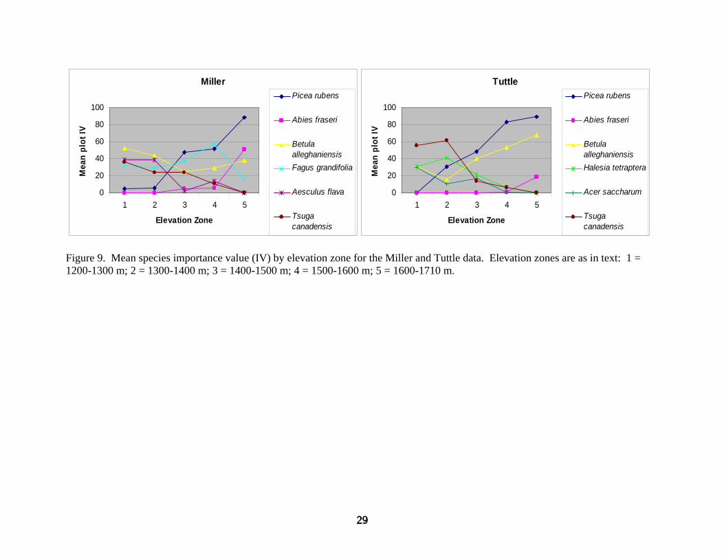
Inspection of dominant species composition by elevation elaborates these and other

differences. For the Miller data, B. alleghaniensis, A. flava, T. canadensis, and F. grandifolia

codominate between 1200 and 1400 m (Figures 7-9). Tsuga canadensis and A. flava generally

decrease in importance with increasing elevation, although T. canadensis remains an important

subdominant through 1500 m. Betula alleghaniensis exhibits a somewhat U-shaped importance

curve with elevation, but remains important between 1400 and 1600 m, while F. grandifolia

increases in importance, and P. rubens emerges as its codominant. Fagus grandifolia is

important primarily because of high densities, and P. rubens clearly dominates by basal area.

Abies fraseri is first present in plots above 1400 m. By 1600-1700 m, P. rubens is the most

important species with A. fraseri and B. alleghaniensis secondarily important. Fagus grandifolia

drops to minimal importance in this zone.

For the Tuttle data, T. canadensis dominates between 1200 and 1300 m with subdominants of

H. tetraptera, B. alleghaniensis, and A. saccharum (Figures 7-9). Tsuga canadensis continues to

dominate between 1300 and 1400 m with a shift in subdominance to H. tetraptera and P. rubens.

Tsuga canadensis, H. tetraptera, and A. saccharum all generally decrease in importance with

increasing elevation and are of minimal or no importance by 1500 m. Picea rubens and B.

alleghaniensis both generally increase in importance with increasing elevation and codominate

between 1400 and 1500 m. Between 1500 and 1700 m, P. rubens and B. alleghaniensis are the

only important species, and P. rubens dominates. Abies fraseri is only minimally present above

1500 m and becomes slightly important by 1600-1700 m because of high density.

Comparison of these species trends with elevation reveals the primary differences in

dominance between the two data sets (Figures 7-9): Abies fraseri and F. grandifolia basal area

and density are much lower in the Tuttle data across all elevations where they occur (zones

26

Figure 7. Mean species basal area (m2/ha) by elevation zone for the Miller and Tuttle data. Elevation zones are as in text: 1 = 1200-1300 m; 2 = 1300-1400 m; 3 = 1400-1500 m; 4 = 1500-1600 m; 5 = 1600-1710 m.

Tuttle

05

101520253035

1 2 3 4 5

Elevation Zone

Mea

n pl

ot b

asal

are

a

Picea rubens

Abies fraseri

Betulaalleghaniensis

Halesiatetraptera

Tsugacanadensis

Miller

05

101520253035

1 2 3 4 5

Elevation Zone

Mea

n pl

ot b

asal

are

a

Picea rubens

Abies fraseri

Betulaalleghaniensis

Aesculusflava

Tsugacanadensis

27 27

Figure 8. Mean species density (stems/ha) by elevation zone for the Miller and Tuttle data. Elevation zones are as in text: 1 = 1200-1300 m; 2 = 1300-1400 m; 3 = 1400-1500 m; 4 = 1500-1600 m; 5 = 1600-1710 m.

Tuttle

0

50100

150

200250

300

1 2 3 4 5

Elevation Zone

Mea

n pl

ot d

ensi

ty

(ste

ms/

ha)

Picea rubens

Abies fraseri

BetulaalleghaniensisFagusgrandifoliaHalesiatetrapteraTsugacanadensisAcersaccharum

Picea rubensMiller

0

50100

150

200250

300

1 2 3 4 5

Elevation Zone

Mea

n pl

ot d

ensi

ty

(ste

ms/

ha)

Abies fraseri

Betulaalleghaniensis

Fagusgrandifolia

Aesculus flava

Tsugacanadensis

28 28

29

by elevation zone for the Miller and Tuttle data. Elevation zones are as in text: 1 = 1200-1300 m; 2 = 1300-1400 m; 3 = 1400-1500 m; 4 = 1500-1600 m; 5 = 1600-1710 m.

Tuttle

0

20

40

60

80

100

1 2 3 4 5

Elevation Zone

Mea

n pl

ot IV

Halesia tetraptera

Acer saccharum

Betulaalleghaniensis

Picea rubens

Abies fraseri

Tsugacanadensis

Miller

0

20

40

60

80

100

1 2 3 4 5

Elevation Zone

Mea

n pl

ot IV

Fagus grandifolia

Aesculus flava

Betulaalleghaniensis

Picea rubens

Abies fraseri

Tsugacanadensis

Figure 9. Mean species importance value (IV)

29

3-5 for A. fraseri and 1-5 for F. grandifolia). Picea rubens density is higher in the Tuttle data for

elevation zones 2-5, most dramatically for zone 4. Basal area, however, is higher only in zones 2

and 4, approximately the same in zone 3, and lower by more than 50% in zone 5. Betula

alleghaniensis basal area and density are higher in the Tuttle data for all but elevation zone 2,

with the most pronounced differences in zones 3-5. Both measures are much lower in elevation

zone 2. There is clear dominance by T. canadensis in zones 1 and 2 for the Tuttle data and more

mixed dominance of several species for the Miller data. Other notable differences in the Tuttle

data include higher density of the disturbance-related Sorbus americana in zone 5 and much

higher basal area and density of several Acer species across all zones, including A.

pensylvanicum, A. spicatum, and A. rubrum.

The increases in overall mean plot density in the Tuttle data for elevation zones 3 and 4 (Figure

6b) are driven largely by higher densities for B. alleghaniensis and P. rubens. Lower basal area

for P. rubens and A. fraseri in zone 5 drives the lower overall mean plot basal area for the Tuttle

data (Figure 6a). However, again, because of the small sample sizes in zones 1 and 2,

differences in dominant species for these zones, as well as the overall differences in mean plot

basal area and density (Figure 6a,b), may reflect inadequate sampling of the diverse community

types at these elevations rather than a temporal shift in dominance.

Community types. Cluster analyses of plots by basal area using Ward’s method and relative

Euclidean distance produced solutions with minimal chaining for the Miller, Tuttle, and

combined Miller-Tuttle data sets. An eight-cluster solution for the combination data set

delineated communities broadly dominated or structured by conifers (P. rubens or T.

canadensis), northern hardwoods (B. alleghaniensis; Quercus rubra; F. grandifolia-A.

saccharum; A. flava-F. grandifolia-B. alleghaniensis; or A. saccharum-H. tetraptera), or

30 30

31

northern hardwoods-conifer (F. grandifolia-P. rubens). Both the P. rubens and T. canadensis

types are well represented in each data set. The A. saccharum-H. tetraptera type consists of

Tuttle plots only. The remaining northern hardwood types, excluding Q. rubra, consist primarily

of either Miller or Tuttle plots, most notably the B. alleghaniensis type, which includes 23.5% of

the Tuttle plots but only 6.3% of the Miller plots. A six-cluster solution for each of the separate

data sets yielded similar types with four common to both Miller and Tuttle, including P. rubens,

B. alleghaniensis, F. grandifolia, and T. canadensis. The Miller data include an A. flava type,

and the Tuttle data include an A. saccharum type and an A. rubrum-Q. rubra type.

Community gradients. Nonmetric multidimensional scaling (NMS) of plot composition by

basal area for the combined data sets yielded a statistically significant (p=0.0196) three-

dimensional solution with a cumulative r2 of 0.829. The data sets encompass a similar range of

compositional variation with much overlap of Miller and Tuttle plots (Figure 10). Elevation as

the dominant compositional gradient is best represented by axis 1, which explains most of the

variance in plot dissimilarity (r2 = 0.473) and is indeed positively correlated with plot elevation (r

= 0.542) (Figure 10). Aspect class and slope are most strongly correlated with axis 3 (r = 0.404

and r = 0.221, respectively), and TCI is the weakest of the topographic variable-axis correlations.

Species-axis correlations indicate which species most structure the compositional gradients

represented by the axes (Table 4). For example, P. rubens and A. fraseri are positively

correlated with axis 1, while lower elevation species such as A. saccharum and A. flava are

negatively correlated. Tsuga canadensis and H. tetraptera most contribute to structure along

axis 2. Wide-ranging species such as B. alleghaniensis and F. grandifolia are correlated with all

three axes. Plotting the combined Ward’s cluster types on the ordination diagram further

illustrates how these dominant species, as indicators of community (and likely

31

T

T

T

T

T

T

T

T

Figure 10. Nonmetric multidimensional scaling (NMS) of the Miller (M) and Tuttle (T) plots combined as one data set. EL_ZONE refers to elevation zones as in text: 1 = 1200-1300 m; 2 = 1300-1400 m; 3 = 1400-1500 m; 4 = 1500-1600 m; 5 = 1600-1700 m. Cumulative r2 = 0.829, final stress 13.77543 (significant by Monte Carlo randomization test, p = 0.0196), final instability 0.00001,. Elevation (m) (vector ELEV_M) is correlated with axes 1 (r = 0.542) and 2 (r = -0.356).

EL_ZONE12345

MM

M

T

TM

M

M

M

T

32

T

T

T

T

T

T

T

T

T

T

T

T

TT

T

T

T

T

TT

T

T

T

M

M

M

M

M

M

MM

M

M M

M

M

M

M

M

MM

MM

M

M

M

M

M

ELEV_M

-1.5

-1.0

-0.5 0.5 1.5

0.0

1.0

Axis 1

Axi

s 2

32

Table 4. Pearson correlations of species basal area with ordination axes for nonmetric multidimensional scaling (NMS) of the combined Miller and Tuttle data. Species abbreviations are as in Table 3. Axis 1 Axis 2 Axis 3 r r2 r r2 r r2

ABFR 0.427 0.182 -0.019 0 -0.094 0.009ACPE 0.039 0.001 -0.071 0.005 0.062 0.004ACRU -0.116 0.013 0.122 0.015 -0.343 0.118ACSA -0.714 0.509 0.007 0 -0.024 0.001ACSP 0.048 0.002 0.004 0 -0.024 0.001AEFL -0.423 0.179 -0.164 0.027 0.298 0.089AMLA -0.002 0 -0.063 0.004 -0.322 0.104BELE -0.057 0.003 0.044 0.002 0.142 0.02BEAL 0.396 0.157 -0.333 0.111 0.661 0.437CADE -0.093 0.009 0.125 0.016 -0.079 0.006CARSP -0.328 0.108 0.196 0.038 0.025 0.001COAL -0.078 0.006 -0.203 0.041 0.04 0.002FAGR -0.47 0.221 -0.408 0.166 -0.461 0.213FRAM -0.155 0.024 -0.065 0.004 0.121 0.015HATR -0.261 0.068 0.563 0.317 0.098 0.01MAAC -0.258 0.066 -0.113 0.013 0.009 0MAFR 0.023 0.001 0.209 0.044 -0.096 0.009PIRU 0.683 0.467 0.239 0.057 -0.164 0.027PRPE 0.164 0.027 -0.083 0.007 0.249 0.062PRSE -0.256 0.066 0.195 0.038 -0.128 0.016QURU -0.242 0.059 0.157 0.025 -0.095 0.009SOAM 0.113 0.013 -0.195 0.038 -0.026 0.001TIHE -0.364 0.133 -0.021 0 0.132 0.017TSCA -0.069 0.005 0.728 0.529 0.202 0.041UNK 0.072 0.005 0.148 0.022 -0.053 0.003

33 33

34

site) types, structure the combined ordination space (Figure 11). In general, the P. rubens and B.

alleghaniensis types are clustered at the high-elevation end of axis 1, and the T. canadensis type

is separated from the F. grandifolia-related clusters by axis 2. The three F. grandifolia types in

turn are distinguished from each other by axis 3 (not shown).

NMS of the Miller and Tuttle data sets separately again yielded statistically significant three-

dimensional solutions with cumulative r2 of .798 and .887, respectively (Figures 12, 13).

Elevation is again the dominant gradient for both data sets. However, this gradient is much more

pronounced in the Tuttle data with a strong correlation of elevation with the primary explanatory

axis (r = 0.764, axis 3), whereas for the Miller data, elevation is most correlated with the weaker

explanatory axes (r = 0.439, axis 2 and r = 0.313, axis 3). Slope and aspect class are instead the

most important topographic variable correlations for the primary Miller axis, and TCI is

relatively uncorrelated with the axes. For the Tuttle data, TCI and aspect class are correlated

with axis 2 and slope with axis 3. Species-axis correlations for the separate ordinations similarly

reveal how the dominant species structure ordination space. For the Miller data, A. fraseri, P.

rubens, A. saccharum, and F. grandifolia most strongly structure axis 2, while T. canadensis and

F. grandifolia are correlated with axis 1 and A. flava with axis 3 (Table 5). For the Tuttle data,

the strongest correlations are concentrated on axis 3, including P. rubens, H. tetraptera, A.

saccharum, and T. canadensis. Fagus grandifolia is correlated with axis 2, B. alleghaniensis

with both axes 2 and 3, and P. rubens and T. canadensis with axis 1 (Table 6). Again the

dominance of these species is illustrated by plotting the separate Ward’s cluster types on the

ordination diagrams (Figures 12, 13), with cluster types more clearly defined here than on the

combined ordination.

34

T

T

T

T

T

T

T

T

T

T

T

T

T

T

T

T

T

T

T

T

T

T

T

T

T

T

T

T

T

T

T

T

T

T

M

M

M

M

M

M

M

M

M

M

M M

M

M

M

M

M

M

M

M

M

MM

MM

M

M

M

M

M

M

M

ELEV_M

M-T_CLUS12348121327

-1.5

-1.0

-0.5 0.5 1.5

0.0

1.0

Axis 1

Axi

s 2

Figure 11. NMS of the combined Miller (M) and Tuttle (T) plots, with cluster types from the combined Miller-Tuttle cluster analysis: 1 = Aesculus flava-Fagus grandifolia-Betula alleghaniensis, 2 = Tsuga canadensis, 3 = Picea rubens, 4 = B. alleghaniensis, 8 = Quercus rubra, 12 = Acer saccharum-Halesia tetraptera, 13 = F. grandifolia-P. rubens, 27 = F. grandifolia-A. saccharum. The vector ELEV_M shows correlation of elevation (m) with axes 1 and 2.

35 35

36

Figure 12. NMS of the Miller data, with cluster types: 1 = Picea rubens, 4 = Quercus rubra, 5 = Fagus grandifolia, 6 = Aesculus flava, 12 = Betula alleghaniensis, 22 = Tsuga canadensis. Cumulative r2 = 0.798, final stress 12.41349 (significant by Monte Carlo test, p = 0.0196), final instability 0.00013. Elevation (m) (vector ELEV_M) is correlated with axes 2 (r = 0.439) and 3 (r = 0.313).

M_CLUS14561222

ELEV_M

-1.5

-1.5

-0.5 0.5 1.5

-0.5

0.5

Axis 2

Axi

s 3

36

ELEV_M

-1.0

-2.0

0.0 1.0

-1.0

0.0

1.0

Axis 2

Axi

s 3

T_CLUS1234812

Figure 13. NMS of the Tuttle data, with cluster types: 1 = Fagus grandifolia, 2 = Tsuga canadensis, 3 = Picea rubens, 4 = Betula alleghaniensis, 8 = Quercus rubra, 12 = Acer saccharum. Cumulative r2 = 0.887, final stress 11.06935 (significant by Monte Carlo test, p = 0.0196), final instability 0.00001. Elevation (m) (vector ELEV_M) is correlated with axis 3 (r = 0.764).

37 37

Table 5. Pearson correlations of species basal area with ordination axes for the Miller NMS. Species abbreviations are as in Table 3. Axis 1 Axis 2 Axis 3

r r2 r r2 r r2

ABFR -0.17 0.029 -0.278 0.078 0.184 0.034 ACPE -0.231 0.054 0.087 0.008 0.053 0.003 ACRU 0.013 0 0.445 0.198 -0.122 0.015 ACSA -0.275 0.076 -0.029 0.001 -0.598 0.357 ACSP -0.003 0 0.109 0.012 0.025 0.001 AEFL -0.296 0.088 -0.065 0.004 -0.385 0.148 AMLA -0.058 0.003 0.37 0.137 0.106 0.011 BELE -0.355 0.126 -0.301 0.09 0.046 0.002 BEAL -0.166 0.028 -0.632 0.399 0.573 0.329 CASP -0.113 0.013 -0.104 0.011 -0.537 0.288 COAL -0.387 0.15 0.028 0.001 -0.006 0 FAGR -0.4 0.16 0.564 0.318 0.128 0.016 HATR 0.445 0.198 -0.043 0.002 -0.695 0.484 MAFR 0.261 0.068 0.178 0.032 -0.142 0.02 PIRU 0.497 0.247 0.253 0.064 0.61 0.372 PRPE -0.102 0.01 -0.301 0.091 0.282 0.079 PRSE -0.143 0.02 0.273 0.075 -0.448 0.201 QURU 0.164 0.027 -0.275 0.076 -0.154 0.024 SOAM -0.167 0.028 0.037 0.001 0.201 0.041 TIHE 0.202 0.041 -0.145 0.021 -0.546 0.298 TSCA 0.538 0.289 -0.125 0.016 -0.546 0.298 UNK 0.233 0.054 0.1 0.01 -0.015 0

38 38

Table 6. Pearson correlations of species basal area with ordination axes for the Tuttle NMS. Species abbreviations are as in Table 3. Axis 1 Axis 2 Axis 3

r r2 r r2 r r2

ABFR 0.222 0.049 0.61 0.372 0.324 0.105ACPE 0.144 0.021 0.063 0.004 -0.114 0.013ACRU -0.239 0.057 -0.239 0.057 -0.356 0.126ACSA -0.185 0.034 -0.687 0.472 -0.413 0.17ACSP 0.033 0.001 0.094 0.009 -0.151 0.023AEFL 0.365 0.133 -0.35 0.122 -0.515 0.265AMLA -0.214 0.046 -0.052 0.003 -0.202 0.041BELE -0.036 0.001 -0.144 0.021 0.333 0.111BEAL 0.323 0.104 0.318 0.101 -0.237 0.056CADE 0.029 0.001 -0.152 0.023 0.127 0.016FAGR -0.518 0.268 -0.659 0.435 -0.36 0.13FRAM 0.126 0.016 -0.135 0.018 -0.388 0.151HATR -0.082 0.007 -0.34 0.115 -0.026 0.001MAAC 0.116 0.013 -0.259 0.067 -0.288 0.083PIRU 0.534 0.285 0.603 0.364 0.449 0.202PRPE 0.183 0.034 0.064 0.004 0.103 0.011QURU -0.363 0.132 -0.344 0.119 -0.342 0.117SOAM -0.08 0.006 0.17 0.029 -0.011 0TIHE -0.123 0.015 -0.182 0.033 -0.437 0.191TSCA 0.536 0.288 -0.005 0 0.48 0.23

39 39

40

The separate ordinations highlight differences in the two data sets noted previously, such as the

decrease in importance of A. fraseri and A. flava and the increase in importance of B.

alleghaniensis and H. tetraptera in the Tuttle data. However, F. grandifolia remains an

important indicator species for community type even though its dominance is much lower. The

communities are organized differently along the dominant gradient (elevation) as well, most

prominently the B. alleghaniensis community type’s closer association in ordination space with

the P. rubens type for the Tuttle data.

A return to the combined ordination diagram with the separate Ward’s cluster types plotted

further illustrates differences in community structure between the Miller and Tuttle data (Figure

14): The Tuttle B. alleghaniensis type is shifted higher along the elevation-dominated axis than

the Miller B. alleghaniensis type and overlaps the Miller P. rubens plots in which A. fraseri was

prominent. While the Tuttle P. rubens type overlaps the same type for Miller, the cluster is more

compact for the Tuttle data. Finally, the T. canadensis type for the Tuttle data is notably separate

in ordination space from the analogous Miller type.

Species-topography relationships. Canonical correspondence analysis (CCA) of the separate

data sets and topographic variables allowed more rigorous comparison of species- and

community-topography relationships in the two data sets. Both ordinations are significant with

similar cumulative variance in species scores explained (~23%) (Table 7). Similar to the NMS

results, the Tuttle data exhibit a stronger relationship with the primary axis than the Miller data.

This difference is reflected in the distribution of topographic variable-axis correlations for the

two data sets: While both ordinations are structured similarly, with elevation, slope, and aspect

class strongly correlated with axes 1, 2, and 3, respectively, elevation is less strongly correlated

and slope and aspect more highly correlated with their respective axes for the Miller data (Table

40

T

T

T

T

T

T

T

T

T

T

T

T

T

T

T

T

T

T

T

T

T

T

T

T

T

T

T

T

T

T

T

T

T

T

M

M

M

M

M

M

M

M

M

M

M M

M

M

M

M

M

M

M

M

M

MM

MM

M

M

M

M

M

M

M

ELEV_M

SEP_CLUS145610122022304080120

-1.5

-1.0

-0.5 0.5 1.5

0.0

1.0

Axis 1

Axi

s 2

Figure 14. NMS of the combined Miller and Tuttle plots, with cluster types from the separate Miller and Tuttle cluster analyses: 1 = Miller Picea rubens, 4 = Miller Quercus rubra, 5 = Miller Fagus grandifolia, 6 = Miller Aesculus flava, 10 = Tuttle F. grandifolia, 12 = Miller Betula alleghaniensis, 20 = Tuttle Tsuga canadensis, 22 = Miller T. canadensis, 30 = Tuttle P. rubens, 40 = Tuttle B. alleghaniensis, 80 = Tuttle Acer rubrum-Q. rubra, 120 = Tuttle Acer saccharum. The vector ELEV_M shows correlation of elevation (m) with axes 1 and 2.

41 41

Table 7. Canonical correspondence analysis (CCA) results for the Miller and Tuttle data. Eigenvalues and species-environment correlations for axis 1 are significant by Monte Carlo randomization test (* p=0.0.2, ** p=0.03, *** p=0.01). Total inertia in the species data was 2.9988 for Miller and 3.1651 for Tuttle.

42

Miller Tuttle Axis 1 Axis 2 Axis 3 Axis 1 Axis 2 Axis 3 Eigenvalue 0.37* 0.188 0.14 0.52*** 0.13 0.09Variance in species data explained (%) 12.40 6.20 4.60 16.40 4.10 2.90Cumulative variance explained (%) 12.40 18.60 23.20 16.40 20.50 23.40Pearson correlations, species-environment 0.77** 0.68 0.61 0.91*** 0.59 0.58Topographic variable correlations

Elevation (m) 0.89 -0.19 0.31 -0.91 0.22 -0.35Aspect class -0.02 0.57 0.82 -0.001 0.54 0.75Slope steepness (%) 0.19 0.93 -0.24 0.21 0.77 -0.45TCI -0.12 0.05 0.21 -0.02 -0.30 0.32

42

7). TCI is the least important topographic variable in both data sets. It should be noted that TCI

was comparable in importance to aspect class for the Tuttle data in the initial ordination.

However, upon inspection of the results, I found that its importance was dependent on one plot

that was an extreme outlier for both TCI value and high basal area for a rare species in the data

set, B. lenta. This outlier compressed the other gradients, making interpretation of the ordination

diagram difficult; removal of this plot from the ordination did not substantially change the

overall result but did reduce the importance of TCI as well as improve ease of interpretation.

Species biplots illustrate the principal similarities and differences between the two data sets

(Figures 15-18). Species are arranged similarly according to their elevation optima (Figures 15,

17); notable shifts include a higher position in the Tuttle data for both B. alleghaniensis and F.

grandifolia, comparable to the position of P. rubens. The shift of Prunus pensylvanica to a high-

elevation optimum reflects the disturbance to A. fraseri forests by the balsam woolly adelgid.

Species arrangements with respect to aspect class are roughly similar between the two data sets

for the important species (Figures 16, 18), with more mesic species, such as A. flava and mesic

Acer species, occupying higher positions. Betula alleghaniensis exhibits more intermediate

optima for both aspect and slope in the Tuttle data. Indeed, the position occupied by this species

in the Tuttle ordination is similar to the position occupied by A. fraseri in the Miller ordination.

In the Tuttle ordination, A. fraseri retains a preference for north-facing aspects but now occupies

primarily flatter, ridgetop slopes. Picea rubens has shifted from a slightly north-facing or

intermediate optimum to a south-facing optimum for aspect class while maintaining an

intermediate position for slope. Fagus grandifolia exhibits a steeper slope optimum in the Tuttle

data, while T. canadensis and H. tetraptera exhibit steeper slope optima in the Miller data. In

general, species positions along the slope vector are difficult to interpret

43 43

BEAL ABFR

PIRU FAGR

BELE

TSCA

HATR

PRPE

AMLA

FRAM

ACRU

ACSA

QURU

AEFL

MAAC

TIHE SOAM

ACPE

ACSP

CADE

Figure 15. Canonical correspondence analysis (CCA) biplot for the Miller data, axes 1 and 3. Species abbreviations are as in Table 3. The vector ELEV_M shows the direction and magnitude (vector length) of correlation with increasing elevation.

ELEV_M

Axis 3 1.5

0.5

Axis 1

-1.5

-1.5

-0.5 0.5 1.5

-0.5

44 44

Figure 16. Canonical correspondence analysis (CCA) biplot for the Miller data, axes 2 and 3. Species abbreviations are as in Table 3. The ASPECT_CLASS and SLOPE% vectors show the direction and magnitude of correlations with increasingly northerly aspect and increasing slope steepness.

igure 16. Canonical correspondence analysis (CCA) biplot for the Miller data, axes 2 and 3. Species abbreviations are as in Table 3. The ASPECT_CLASS and SLOPE% vectors show the direction and magnitude of correlations with increasingly northerly aspect and increasing slope steepness.

45

BEAL

ABFR PIRU FAGR

BELE

TSCA

HATR

PRPE

AMLA

FRAM

ACRU

ACSA

QURU

AEFL

MAAC

TIHE

SOAM

ACPE

ACSP

CADE

ASPECT_CLASS

SLOPE%

-1.5 -0.5

-1.5

-0.5

0.5

1.5

Axis 3

0.5 1.5

Axis 2

45

46

Figure 17. Canonical correspondence analysis (CCA) biplot for the Tuttle data, axes 1 and 3. The ELEV_M vector shows the direction and magnitude (vector length) of correlation with increasing elevation.

ABFR

ACPE

ACRU

ACSA

ACSP

AEFL

AMLA

BELE

BEAL

CASP

COAL

FAGR

HATR

MAFR

PIRU

PRPE

PRSE

QURU

SOAM

TIHE

TSCA

UNK

ELEV_M

Axis 1

2.0 1.0

Axis 3

0.0

-0.5

-1.5

1.5

0.5

-1.0 -2.0

46

ABFR

ACPE

ACRU

ACSA

ACSP

Figure 18. Canonical correspondence analysis (CCA) biplot for the Tuttle data, axes 2 and 3. The ASPECT_CLASS and SLOPE% vectors show the direction and magnitude of correlations with increasingly northerly aspect and increasing slope steepness.

AEFL

AMLA

BELE

BEAL

CASP

COAL

FAGR HATR

MAFR

PIRU

PRPE

PRSE

QURU

SOAM

TIHE

TSCA

UNK

ASPECT_CLASS

SLOPE%

Axis 3 1.5

0.5

Axis 2

-1.0

-1.5

0.0 1.0

-0.5

47 47

except for the widespread species mentioned above, most likely because of small overall sample

size combined with a sampling design unstratified by slope.

48 48

Chapter 5: Discussion

Ecotonal change. Results of this study imply an ecotonal forest that is in transition,

recovering from disturbance – because of the significantly higher mean plot stem density, the

similar mean plot basal area, and higher mean plot species richness. Change in stand attributes is

most pronounced between 1400 and 1600 m elevation via increased density and between 1600

and 1700 m elevation via decreased basal area. Shifts in dominant and subdominant species

reflect primarily the most recent, acute disturbances: decimation of Abies fraseri by the balsam

woolly adelgid since its spread to the park in the 1960s and high mortality of Fagus grandifolia

from beech bark disease (Cryptococcus fagisuga and Nectria spp.) since its discovery in the park

in 1993. Fagus grandifolia, a formerly widespread dominant species, has been reduced to a

subdominant species, while A. fraseri, formerly a high-elevation dominant, is no longer even

subdominant; both species have contracted distributions. Picea rubens and Betula

alleghaniensis, mid- to high-elevation associates of both F. grandifolia and A. fraseri, not only

remain dominant but occur more frequently in plots. A low- to mid-elevation species, Halesia

tetraptera, has attained subdominant, widespread status, while two lower-elevation associates of

F. grandifolia, Aesculus flava and Acer saccharum, are not dominant or subdominant in the

Tuttle data but persist in occurrence.

Changes in size-class distributions confirm the forest recovery, showing a dramatic overall

increase in the smallest size class (10.1–30.3 cm dbh) with reductions in size class 3. Again, P.

rubens, B. alleghaniensis, and H. tetraptera show strong responses to the losses of A. fraseri and

F. grandifolia with increased density in the two smallest size classes. However, size-class

49 49

distributions imply that other low- to mid-elevation species, including Tsuga canadensis, A.

saccharum, and A. flava, also have responded to these losses to varying degrees in the smallest

size class, and T. canadensis notably occurs twice as frequently in plots. Strong responses of

Acer pensylvanicum, Acer spicatum, and Acer rubrum in the smallest size class are accompanied

by newly widespread distribution of these species across the ecotone. High stem densities for

small, short-lived understory trees, such as A. pensylvanicum and A. spicatum, support the

interpretation that these forests are actively responding to the recent acute disturbances. Acer

rubrum and H. tetraptera have increased in size class 3, indicating possibly fast growth of these

species as well as high survivorship into larger structural classes. In contrast, the historically

more dominant canopy species (P. rubens, T. canadensis, A. saccharum, and A. flava) show

apparent decreases in size class 3 accompanied by minimal change in the largest size class.

Species abundance differences by elevation illustrate important compositional changes within

the ecotone. The shift to dominance by P. rubens still occurs between 1400 and 1500 m.

However, what was once a more subtle shift – which remained complex with increasing

elevation because of the mixed importance of F. grandifolia and A. fraseri – has become a more

abrupt shift to dominance by P. rubens and B. alleghaniensis. Closer inspection reveals that both

P. rubens and B. alleghaniensis have increased in dominance most dramatically between 1500

and 1600 m, while between 1400 and 1500 m, P. rubens dominance has not changed; rather, B.

alleghaniensis appears to have replaced F. grandifolia in dominance, and T. canadensis and

other hardwoods remain subdominant. Between 1600 and 1700 m, P. rubens has maintained its

dominance through an increase in density, despite a decrease in basal area that may be

attributable to increased windthrow or winter climate exposure following mass mortality of

50 50

surrounding A. fraseri. At the lower elevations, dominance remains a more complex assortment

of T. canadensis and hardwoods.

Although the species structuring the four main community clusters (P. rubens, B.

alleghaniensis, T. canadensis, and F. grandifolia) are the same in the two data sets, cluster

composition is actually quite different between the two data sets. Abies fraseri has decreased in

the P. rubens type but has slightly increased (from not present to present) in the B. alleghaniensis

and F. grandifolia types. For B. alleghaniensis, this likely reflects increased dominance in high-

elevation sites that once were dominated by A. fraseri. For F. grandifolia, this may reflect

restriction of dominance to mainly higher elevation sites where P. rubens is codominant,

whereas the typical F. grandifolia-mixed northern hardwood type that is most prominent in the

Miller data is nearly absent from the Tuttle data, perhaps partially a result of small sample size in

the lower elevations as well as transition of formerly F. grandifolia-dominated plots to B.

alleghaniensis- or other hardwood-dominated plots. Fagus grandifolia indeed has decreased

across all cluster types, including its own, except for a likely insignificant increase in the P.

rubens cluster, although it should be noted that perhaps F. grandifolia responded to the loss of A.

fraseri in both the P. rubens and P. rubens-F. grandifolia types before the onset of beech bark

disease. Betula alleghaniensis has increased across three of the four main cluster types and has

decreased in the T. canadensis cluster. However, this likely reflects the fact that the Miller

cluster consists of T. canadensis-mixed northern hardwood plots, whereas the Tuttle cluster

consists of high-basal-area T. canadensis-H. tetraptera plots with minimal representation by

other northern hardwoods; these plots may represent old-growth T. canadensis outliers, but the

subdominance of H. tetraptera and the presence of A. pensylvanicum and A. rubrum indicate a

response to gap disturbance. The increase of Acer spp. (excluding A. saccharum) across the four

51 51

main cluster types indicates recent gap disturbances across the entire ecotone. The Tuttle A.

saccharum-dominated plots, however, lack any obviously disturbance-related species, indicating

that these may be old-growth stands unaffected by recent acute disturbances. It should be noted

that while P. rubens still definitively dominates the P. rubens cluster, basal area of all conifer

species including P. rubens has decreased while that of nearly all northern hardwood species,

particularly B. alleghaniensis and H. tetraptera, has increased in this cluster.

Both direct and indirect gradient analysis support the interpretation of ecotonal reorganization,

with B. alleghaniensis increasing at higher elevation with contraction of A. fraseri, F. grandifolia

contracting to higher elevation as it declines, and P. rubens maintaining dominance in many

plots but perhaps yielding to increased presence of northern hardwoods. Stronger correlation of

Tuttle plot composition with elevation suggests that the modern ecotone is more strongly

structured along the elevation gradient, and this is supported by the more pronounced dominance

of P. rubens and B. alleghaniensis above 1400 m as well as decreased mean plot evenness.

Further, P. rubens, B. alleghaniensis, F. grandifolia, and A. pensylvanicum now occupy similar

optima along the CCA elevation gradient. Acer rubrum likewise has shifted to a higher-

elevation optimum. While most frequently occurring species maintained similar aspect

preferences (but varied in slope), P. rubens and B. alleghaniensis became polarized, with P.

rubens dominating more frequently on south-facing aspects and B. alleghaniensis almost

exclusively on north-facing aspects; P. rubens’s optimum accordingly shifted from an

intermediate to a south-facing aspect, while B. alleghaniensis’s optimum became more

intermediate but remained north-facing.

Related findings. Most studies of impacts to the high-elevation spruce-fir forests of the Great

Smoky Mountains and southern Appalachians have focused within the spruce-fir-dominated

52 52

forest itself, often at the several-plot or stand level, sometimes comparing two or more widely

spaced locations (e.g., Busing et al. 1988, Smith and Nicholas 1998). Many of these empirical

studies have focused on A. fraseri mortality, regeneration, and recruitment after infestation by

the balsam woolly adelgid, generally documenting overall recruitment success and persistence of

A. fraseri following infestation, although the long-term dynamics of the balsam woolly adelgid

and A. fraseri abundance are uncertain (Dale et al. 1991, Smith and Nicholas 2000). Harmon et

al. (1983) did predict an increase in B. alleghaniensis in dense A. fraseri stands after the balsam

woolly adelgid. However, Busing and Clebsch (1987) simulated stand dynamics for P. rubens,

A. fraseri, and B. alleghaniensis and predicted that P. rubens would dominate upon exogenous

disturbance to A. fraseri, whereas B. alleghaniensis would dominate only upon exogenous

disturbance to both A. fraseri and P. rubens. Busing et al. (1988) then documented increased

biomass/dominance of P. rubens and decreased biomass/subdominance of B. alleghaniensis at

two sites above 1700 m following balsam woolly adelgid infestation but subsequently

documented increased mortality of P. rubens from increased exposure to windthrow in the same

study area in 1993 (Busing and Pauley 1994), in the absence of abnormal wind velocities or

declines in radial growth of P. rubens. The paucity of tree species at the highest elevations and

the fact that most of these studies were conducted over a decade ago limits conclusions about

long-term survival of spruce-fir forests, particularly following the balsam woolly adelgid.

Another group of studies has focused on the detrimental effects of atmospheric deposition on

P. rubens in the southern Appalachians (see McLaughlin et al. 1994 for a brief review), again

focused mostly on P. rubens in the spruce-fir zone and often based on dendrochronological data.

One of the most recent of these (Webster et al. 2004) links climate variability and regional

atmospheric pollution inputs over the last century to declines in radial growth of P. rubens at two

53 53

GRSM spruce-fir sites at 1500 and 1800 m elevation; this same study speculates that a 1990s

spike in radial growth was a response to mortality of A. fraseri from the balsam woolly adelgid.

These studies do not document increased mortality directly from atmospheric inputs and are not

integrated with studies of similar effects on co-occurring species, so again, the results are

inconclusive regarding the long-term survival of P. rubens in spruce-fir forests.

While the intention of this study is to document ecotonal change over 70 years as an additional

route to evaluating persistence of high-elevation spruce-fir forests in GRSM under multiple

impacts, the results seem to capture primarily the effects of recent declines in two ecotone-

related species, A. fraseri and F. grandifolia. This likely masks any changes occurring between

the 1930s and 1970s as well as changes from other ongoing impacts. Ecotone-focused studies

from the intervening time period would be useful but are scarce, with three exceptions: 1)

Schofield (1960) collected plot data in ecotonal transects for 10 ecotonal “types”, including

“virgin”, cut, and burned areas. Schofield’s study included sites with dense Rhododendron

maximum understory, and he considered P. rubens-dominated sites ecotonal. However, although

only anecdotally comparable, his results echo site preferences found for several species in the

Miller data (Busing et al. 1993) and Tuttle data: Across “types”, P. rubens, F. grandifolia, and

T. canadensis attained consistently higher basal area on southern slopes, whereas Betula

alleghaniensis basal area was higher on northern slopes. However, A. fraseri also attained

consistently higher basal area on southern slopes, in contrast to the north-facing site preference

found in the Miller and Tuttle samples of this study. Also of interest, B. alleghaniensis basal

area was greater on slopes with evidence of cutting, while P. rubens and F. grandifolia basal

area was lower on these sites. Schofield observed that the ecotone occurred at higher elevation

on south-facing slopes, which he attributed to cutting and burning. 2) DeSelm (1970s) collected

54 54

plot data along elevational transects in the westernmost ecotonal watersheds of GRSM but did

not publish results of any analysis. 3) More recently, Hayes (2002) used a remotely sensed map

of GRSM spruce-fir extent (date not specified) and Pyle’s (1984) logging history map to

investigate the interactive effects of logging history, aspect, and potential insolation on spruce-fir

presence in a 1-km buffer straddling the boundary of the spruce-fir zone. His results suggested

that the mean elevation of sites with spruce-fir present was higher on logged south-facing slopes.

Perhaps more useful are studies of GRSM forest types related to the ecotone, such as northern

hardwood cove, T. canadensis, and F. grandifolia forests, particularly those studies investigating

change over time using the Miller or other historical data. Busing (1989) resampled two of

Stanley Cain’s 1935 cove hardwood plots (Cain unpublished in Busing 1989), sampled

approximately five years after mortality of Castanea dentata from chestnut blight

(Cryphonectria parasitica) at both sites. Total stand and A. saccharum basal area increased at

both sites, and either T. canadensis or H. tetraptera increased in basal area at each of the sites;

these results are similar to the findings of Woods and Shanks (1959) in their study of post-blight

forest dynamics in GRSM. In 1998, Knebel (1999) approximately relocated and resampled 20

Miller T. canadensis-dominated plots, including some plots between 1200 and 1500 m elevation.

She found that while T. canadensis sapling density remained the same over the 60 years, T.

canadensis basal area and density decreased overall, especially in the larger size classes. As in

my results, species such as A. pensylvanicum, H. tetraptera, and A. rubrum dramatically

increased in sapling densities and overall importance. Similar dramatic increases in F.

grandifolia sapling density and importance indicate that Knebel’s plots had experienced little to

no mortality from beech bark disease at that time. Knebel attributed these changes primarily to

the reduction of C. dentata frequency from six to zero of the 20 plots. In contrast, Jenkins

55 55

(personal communication 2006) commented that T. canadensis had increased in the understory in

the park as a result of fire suppression, although fire was likely uncommon at the higher

elevations in the eastern park.

Finally, between 2000 and 2004, Vandermast (2005) sampled high-elevation F. grandifolia

forests to compare to both F. grandifolia forests in the Miller data and in 1970s plots. He found

increases in non-diseased, co-occurring northern hardwood species and P. rubens, particularly in

the smallest size classes, similar to my results and likely indicating release following mortality of

F. grandifolia from beech bark disease. He noted a decline in overall A. flava abundance similar

to my results. The striking finding in his study was greater abundance of F. grandifolia in the

1970s plots compared to the Miller plots and, surprisingly, abundance similar to that of the

Miller data in 2000-2004; he concluded that F. grandifolia forests had been aggrading since the

1930s and then had declined with the onset of mortality from beech bark disease.

Summary of impacts and consideration of future dynamics. While the results of this study

suggest recovery and reorganization of ecotonal stands, most obviously from the recent losses of

A. fraseri and F. grandifolia, direct causes are by no means easily mapped onto the effects

shown here and are not the intent of this study. Vandermast’s study (2005) deftly illustrates the

likelihood that the recent changes observed (or not) in the ecotone are masking other

compositional and structural changes that had occurred since the 1930s and that may continue or

interact with the observed changes. For example, the findings of Busing (1989) and Knebel

(1999) support the possibility that some changes in the ecotone since the 1930s are attributable to

recovery from chestnut blight; indeed, inspection of the Miller data reveals unlogged, unburned

C. dentata-dominated plots between 1200 and 1700 m in the study area watersheds that were

56 56

excluded from comparison as non-northern hardwood plots (or perhaps plots that did not border

any spruce-fir forest).

In the case of the diverse range of community and site types encompassed by the ecotone,

current forest composition may reflect different stages of impact and recovery from a long list of

direct, discrete impacts, including release from selective cutting and grazing; fire suppression;

removal of C. dentata by chestnut blight; increased exposure to windthrow from the onslaught of

canopy openings; seedling, root, and soil disturbance by non-native wild boars (present in the

eastern park for the past 10-15 years; Peter White, personal communication 2006); and the usual

array of natural disturbances such as hurricanes, flooding, and ice storms. Ongoing,

continuously distributed impacts further complicate investigation of change: Atmospheric

deposition may affect health of ecotonal species directly through foliar damage from ozone or

indirectly through biogeochemistry (McLaughlin 1994). Recently documented climate change,

whether transient or a long-term trend, can alter both the dominant environmental gradients

(temperature and precipitation) and the disturbance gradients that structure these montane forests

(Harmon et al. 1983). Webster et al. (2004) found a recent shift in long-term temperature-

precipitation data for GRSM from cycles of warm/wet and cool/dry to warm/dry and cool/wet.

Anchukaitis et al. (2006) support this through a finding of increased drought sensitivity of

southern Appalachian conifers as recorded in tree rings. An impending decline in T. canadensis

upon full infestation of GRSM by the hemlock woolly adelgid (Adelges tsugae) will impose yet

another cycle of targeted mortality and canopy openings on the ecotone. The spatial and

temporal extents of these factors overlap, and processes likely interact (e.g., the effect of

temperature-precipitation cycles on dynamics of the hemlock woolly adelgid).

57 57

With such complexity, what can be said about the GRSM deciduous-coniferous ecotone?

Based on the results of this study, the abundance and distribution of P. rubens seem at least

preserved in the ecotone, pending success of enough of the abundant small trees. Abies fraseri

appears to be persisting in a diminished state at the highest elevations. It is unknown whether B.

alleghaniensis will persist in dominating former A. fraseri forests, particularly on north-facing

slopes. Perhaps P. rubens will survive under protection of the B. alleghaniensis canopy and

succeed to dominance. However, in the meantime, if drought stress begins to induce mortality,

P. rubens could diminish on the south-facing aspects it now dominates. One can also envision

an assortment of exogenous stressors upon P. rubens that could combine to result in increased

mortality, reduced suppression tolerance, or reproductive/establishment failure, perhaps leading

to widespread decline. Such stressors may affect other ecotonal species, too, however. The

perceived increase in this study of northern hardwood species in P. rubens-dominated stands

may indicate a transition in progress. Picea rubens and/or A. fraseri already may be persisting in

GRSM beyond their respective climate or competitive envelopes, as perhaps evidenced by the

near-restriction of A. fraseri to north-facing, high-elevation slopes above 1500 m elevation, when

the species formerly showed, in the Miller data, a slight affinity for north-facing sites but was

abundant on both aspects. In contrast, P. rubens may expand at the expense of another species if

it benefits from release on T. canadensis sites affected by the hemlock woolly adelgid.

Is the GRSM spruce-fir ecotone important? Time will tell, and this study may contribute to

longer term research and monitoring of the entire ranges of P. rubens and A. fraseri in GRSM.

A wish list for future study of the GRSM spruce-fir ecotone could include a more complete

sample of the ecotone, including Rhododendron species-dominated sites and stratification by

land use/disturbance history; the establishment of physically marked permanent plots to

58 58

accompany GIS coordinates for more reliable repeat sampling; attempted relocation of historical

plots; and the collection of more site and vegetation data (e.g., tree cores for dendroecological

analysis). It seems feasible that understanding the prospects for P. rubens and A. fraseri

persistence in the face of exogenous stressors could inform conservation efforts. For example,

this study’s finding of A. fraseri’s current near-restriction to north-facing sites above 1500 m

may mean limited re-expansion pathways should surviving A. fraseri forests fully recover from

the balsam woolly adelgid. Likewise, this knowledge could inform site selection for spruce-fir–

related research, conservation, or restoration projects. Beyond conservation in GRSM and this

study in particular, attempting to unravel montane deciduous-coniferous ecotonal dynamics may

forward our understanding of complex ecological dynamics in the context of global change.

59 59

References

Allen, C.D., and D.D. Breshears. 1998. Drought-induced shift of a forest-woodland ecotone: rapid landscape response to climate variation. Proceedings of the National Academy of Sciences 95: 14839-14842. Beniston, Martin. 1994. Mountain Environments in Changing Climates. Routledge, London. Benjamini, Y., and Y. Hochberg. 1995. Controlling the false discovery rate: a practical and powerful approach to multiple testing. Journal of the Royal Statistical Society, Series B (Methodological) 57(1): 289-300. Beven, K.J., and M.J. Kirkby. 1979. A physically based, variable contributing area model of basin hydrology. Hydrological Sciences Bulletin 24(1): 43-69. Burns, R.M., and B.H. Honkala, technical coordinators. 1990. Silvics of North America: 1. Conifers; 2. Hardwoods. Agriculture Handbook 654, vol. 2. U.S. Department of Agriculture, Forest Service, Washington, DC. Busing, R.T. 1989. A half century of change in a Great Smoky Mountains cove forest. Bulletin of the Torrey Botanical Club 116(3): 283-288. Busing, R.T., and E.E.C. Clebsch. 1987. Application of a spruce-fir forest canopy gap model. Forest Ecology and Management 20(1-2): 151-169. Busing, R.T., E.E.C. Clebsch, C.C. Eagar, and E.F. Pauley. 1988. Two decades of change in a Great Smoky Mountains spruce-fir forest. Bulletin of the Torrey Botanical Club 115: 25-31. Busing, R.T., and E.F. Pauley. 1994. Mortality trends in a southern Appalachian red spruce population. Forest Ecology and Management 64: 41-45. Busing, R.T., P.S. White, and M.D. MacKenzie. 1993. Gradient analysis of old spruce-fir forests of the Great Smoky Mountains circa 1935. Canadian Journal of Botany 71: 951-958. Cain, S.A. 1935. Ecological studies of the vegetation of the Great Smoky Mountains. II. The quadrat method applied to sampling spruce and fir forest types. American Midland Naturalist 16: 566-584. Dale, V.H., R.H. Gardner, D.L. DeAngelis, C.C. Eagar, and J.W. Webb. 1991. Elevation-mediated effects of balsam woolly adelgid on southern Appalachian spruce-fir forests. Canadian Journal of Forest Research 21: 1639-1648. Delcourt, P.A., and H.R. Delcourt. 1998. Paleoecological insights on conservation of biodiversity: a focus on species, ecosystems, and landscapes. Ecological Applications 8(4): 921-934.

60 60

DeSelm, H.R. 1970s. Unpublished plot data for the spruce-fir ecotone in Great Smoky Mountains National Park. Faith, D.P., P.R. Minchin, and L. Belbin. 1987. Compositional dissimilarity as a robust measure of ecological distance. Vegetatio 69: 57-68. Fernandez, I.J. 1992. Characterization of eastern U.S. spruce-fir soils. In Eagar, C., and M.B. Adams, editors, Ecology and Decline of Red Spruce in the Eastern United States. Springer-Verlag, New York. Harmon, M.E., S.P. Bratton, and P.S. White. 1983. Disturbance and vegetation response in relation to environmental gradients in the Great Smoky Mountains. Vegetatio 55: 129-139. Hayes, M.D. 2002. GIS modeling of spruce/fir distribution and its lower boundary in the Great Smoky Mountains National Park. M.A. Thesis, University of North Carolina at Chapel Hill, Chapel Hill, NC. Knebel, L.G. 1999. Changes in old growth hemlock forests of the Cataloochee watershed in the Great Smoky Mountains National Park: preparing for the arrival of the hemlock woolly adelgid (Adelges tsugae). M.S. Thesis, Western Carolina University, Cullowhee, NC. Kruskal, J.B. 1964. Multidimensional scaling by optimizing goodness-of-fit to a nonmetric hypothesis. Psychometrika 29(1): 1-27. Hofgaard, A. 1997. Inter-relationships between treeline position, species diversity, land use and climate change in the central Scandes Mountains of Norway. Global Ecology and Biogeography Letters 6: 419-429. Holland, S.M., and M. Patzkowsky. 2006. Abstract: Reevaluating the utility of detrended correspondence analysis and non-metric multidimensional scaling for ecological ordination. Presentation at the 2006 Annual Meeting of the Geological Society of America, October 22-25, 2006. Golden, M.S. 1981. An integrated multivariate analysis of forest communities of the central Great Smoky Mountains. American Midland Naturalist 106: 37-53. Gosz, J.R. 1992. Gradient analysis of ecological change in time and space: implications for forest management. Ecological Applications 2(3): 248-261. Grau, H.R., and T.T. Veblen. 2000. Rainfall variability, fire and vegetation dynamics in neotropical montane ecosystems in north-western Argentina. Journal of Biogeography 27: 1107-1121. Jenkins, M.A. 2006. Personal communication, UNC Ecology Curriculum seminar. University of North Carolina at Chapel Hill, Chapel Hill, NC.

61 61

Jobe, R.T. 2006. Biodiversity and scale: determinants of species richness in Great Smoky Mountains National Park. Ph.D. Dissertation, University of North Carolina at Chapel Hill, Chapel Hill, NC. Kent, M., and P. Coker. 1992. Vegetation description and analysis: a practical approach. John Wiley & Sons, West Sussex, England. Kunze, M. 2003. Great Smoky Mountains database (CD). Great Smoky Mountains National Park, National Park Service, U.S. Department of Interior. Kupfer, J.A., and D.M. Cairns. 1996. The suitability of montane ecotones as indicators of global climatic change. Progress in Physical Geography 20(3): 253-272. MacKenzie, M.D., and P.S. White. 1998. Vegetation of Great Smoky Mountains National Park, 1935-1938. Castanea 63(3): 323-336. Madden, M., R. Welch, T. Jordan, P. Jackson, R. Seavey, and J. Seavey. 2004. Digital Vegetation Maps for the Great Smoky Mountains National Park. Final Report to the U.S. Dept. of Interior, National Park Service, Cooperative Agreement Number 1443-CA-5460-98-019. Center for Remote Sensing and Mapping Science, The University of Georgia, Athens, GA. Malanson, G.P. 1999. Considering complexity. Annals of the Association of American Geographers 89(4): 746-753. Masek, J.G. 2001. Stability of boreal forest stands during recent climate change: evidence from Landsat satellite imagery. Journal of Biogeography 28: 967-976. McCune, B., and M.J. Mefford. 1999. PC-ORD. Multivariate analysis of ecological data. Version 4.37. MjM Software, Gleneden Beach, OR. McLaughlin, S.B., T.J. Blasing, and D.J. Downing. 1994. Two hundred year variation of southern red spruce radial growth as estimated by spectral analysis: comment. Canadian Journal of Forest Research 24: 2299-2304. McLaughlin, S.B., M.G. Tjoelker, and W.K. Roy. 1993. Acid deposition alters red spruce physiology – laboratory studies support field observations. Canadian Journal of Forest Research 23(3): 380-386. Moore, H.L. 1988. A Roadside Guide to the Geology of the Great Smoky Mountains National Park. The University of Tennessee Press, Knoxville, TN. Noble, I.R. 1993. A model of the responses of ecotones to climate change. Ecological Applications 3(3): 396-403. Oosting, H.J., and W.D. Billings. 1951. A comparison of virgin spruce-fir in the northern and southern Appalachian systems. Ecology 32: 84-103.

62 62

Parker, A.J. 1982. The topographic relative moisture index: an approach to soil moisture assessment in mountain terrain. Physical Geography 3: 160-168. Payette, S., M.J. Fortin, and I. Gamache. 2001. The subarctic forest-tundra: the structure of a biome in a changing climate. BioScience 51(9): 709-718. Peart, D.R., N.S. Nicholas, S.M. Zedaker, M.M. Miller-Weeks, and T.G. Siccama. 1992. Condition and recent trends in high-elevation red spruce populations. In Eagar, C., and M.B. Adams, editors, Ecology and Decline of Red Spruce in the Eastern United States. Springer-Verlag, New York. Pyle, C. 1984. Pre-park disturbance in the spruce-fir forests of Great Smoky Mountains National Park. In P.S. White, editor, The Southern Appalachian Spruce-Fir Ecosystem: Its Biology and Its Threats, Research/Resource Management Report SER-71, p. 115-130. National Park Service, U.S. Department of Interior. Pyle, C. 1988. The type and extent of anthropogenic vegetation disturbance in the Great Smoky Mountains before National Park Service acquisition. Castanea 53(3): 183-196. Schofield, W.B. 1960. The ecotone between spruce-fir and deciduous forest in the Great Smoky Mountains. Ph.D. Dissertation, Duke University, Durham, NC. Smith, G.F., and N.S. Nicholas. 1998. Patterns of overstory composition in the fir and fir-spruce forests of the Great Smoky Mountains after balsam woolly adelgid infestation. American Midland Naturalist 139(2): 340-352. Smith, G.F., and N.S. Nicholas. 2000. Size- and age-class distributions of Fraser fir following balsam woolly adelgid infestation. Canadian Journal of Forest Research 30(6): 948-57. ter Braak, C.J.F. 1987. The analysis of vegetation-environment relationships by canonical correspondence analysis. Vegetatio 69: 69-77. Urban, D.L. 2000. Using model analysis to design monitoring programs for landscape management and impact assessment. Ecological Applications 10(6): 1820-1832. Vandermast, D.B. 2005. Disturbance and long-term vegetation change in the high-elevation deciduous forests of Great Smoky Mountains National Park. Ph.D. Dissertation, University of North Carolina at Chapel Hill, Chapel Hill, NC. Ward, Jr., J.H. 1963. Hierarchical grouping to optimize an objective function. Journal of the American Statistical Association 58(301): 236-244. Weakley, Alan S. 2007. Flora of the Carolinas, Virginia, Georgia, and surrounding areas, working draft of 11 January 2007. University of North Carolina Herbarium, University of North Carolina at Chapel Hill, Chapel Hill, NC, available at http://herbarium.unc.edu/flora.htm.

63 63

Webster, K.L., I.F. Creed, N.S. Nicholas, and H. Van Miegroet. 2004. Exploring interactions between pollutant emissions and climatic variability in growth of red spruce in the Great Smoky Mountains National Park. Water, Air, and Soil Pollution 159: 225-248. Welch, R., M. Madden, and T. Jordan. 2002. Photogrammetric and GIS techniques for the development of vegetation databases of mountainous areas: Great Smoky Mountains National Park. ISPRS Journal of Photogrammetry & Remote Sensing 57: 53-68. White, P.S., and R.T. Busing. 1993. Vegetation monitoring and an assessment of past studies. In LTERM: Long-term monitoring and research in Great Smoky Mountains National Park, Technical Report NPS/SERGRSM/NRTR-93/10. National Park Service, U.S. Department of the Interior. White, P.S., and C.V. Cogbill. 1992. Spruce-fir forests of eastern North America. In Eagar, C., and M.B. Adams, editors, Ecology and Decline of Red Spruce in the Eastern United States. Springer-Verlag, New York. White, P.S. 2004. Personal communication. Whittaker, R.H. 1956. Vegetation of the Great Smoky Mountains. Ecological Monographs 26: 1-80. Woods, F.W., and R.E. Shanks. 1959. Natural replacement of chestnut by other species in the Great Smoky Mountains National Park. Ecology 40(3): 349-361. Woodward, F.I. 1993. The lowland-to-upland transition – modelling plant response to environmental change. Ecological Applications 3(3): 404-408.

64 64